CIRJE Discussion Papers can be downloaded without charge from:

http://www.e.u-tokyo.ac.jp/cirje/research/03research02dp.html

Discussion Papers are a series of manuscripts in their draft form. They are not intended for

circulation or distribution except as indicated by the author. For that reason Discussion Papers may

not be reproduced or distributed without the written consent of the author.

CIRJE-F-289

Accounting for Human Capital and Weak Identification inEvaluating the Epstein-Zin-Weil Non-Expected

Utility Model of Asset Pricing

Qiang ZhangUniversity of Memphis

July 2004

Accounting for Human Capital and Weak Identification in Evaluating the Epstein-Zin-Weil Non-Expected Utility Model of

Asset Pricing1

QIANG ZHANG Department of Economics

University of Memphis Memphis, TN 38152

qzhang2@memphis.edu

Tel.: (901) 678 4627

This Version: June 20, 2004

Abstract

In this paper, I first develop a new approach to estimating the return on the aggregate wealth portfolio

that accounts for human capital and financial assets other than stocks. Using the estimated return on

the wealth portfolio and the quarterly U.S. aggregate data on consumption and asset returns from 1959

to 2001, I then test the asset pricing and consumption implications of the Epstein and Zin (1991) and

Weil (1990) model by employing the weak-identification robust tests of Stock and Wright’s (2000) in

the context of continuous updating generalized method of moments. In contrast with previous studies

that ignored human capital and weak identification in evaluating this model, I find that its asset pricing

implications cannot be rejected at conventional significance levels for reasonable parameter values.

For example, the 95% confidence sets for unknown parameters include values of the relative risk

aversion around 2 or lower, values of the elasticity of intertemporal substitution for consumption

closely around 1, and the time discount factor around 0.987. Some of these parameter value

combinations are able to simultaneously match the average equity premium and the average riskfree

rate in the data. Furthermore, they imply that the dominant determinant of the equity premium is,

surprisingly, the volatility of stock returns, the risk factor in the traditional capital asset pricing model.

Key Words: Asset Pricing, Non-Expected Utility Preferences, Human Capital, Weak Identification

1 I thank John Conlon, Bill Smith, the seminar audience at University of Memphis, Ole Miss, and University of Tokyo, and the participants of the 2004 Midwest Macroeconomics Meetings held at Iowa State University for helpful comments on different versions of this paper. Bill Smith also corrected the stylistic errors in the paper, for which I am grateful. I thank Jonathan Wright for sharing with me some of the GAUSS and Matlab programs used in his paper with James Stock, and Sydney Ludvigson for providing the price deflator data used in a joint paper of hers with Martin Lettau. All remaining errors are mine.

0

1. Introduction

The consensus view in the asset pricing literature on the Epstein and Zin (1991) and Weil

(1990) non-expected utility model (henceforth the EZW model) is that it cannot resolve the equity

premium puzzle (Mehra and Prescott (1985)) and the related risk-free rate puzzle. See e.g. Weil

(1989), Kocherlakota (1996), and Campbell (2003).2 The goal of this paper is to fully evaluate

the EZW model to see if this consensus still holds. A full evaluation that incorporates the major

relevant developments in the asset pricing literature and the econometric literature should include

the following three elements: to account for the presence in the wealth portfolio of human capital

and financial assets that are usually ignored in an empirical analysis, such as private (i.e.

noncorporate) equity, housing, and consumer durable goods; to account for weak identification in

the estimation and testing; and to estimate all the parameters and test both the consumption and

asset pricing implications of this model. Viewed in this light, the previous studies of the EZW

model all lack at least one of these three elements, although they are very useful in fleshing out

the properties and implications of the model. See, among others, Attanasio and Weber (1989),

Weil (1989), Bufman and Leiderman (1990), Kocherlakota (1990a, 1996), Epstein and Zin

(1991), Kandel and Stambaugh (1991), Cochrane and Hansen (1992), Cecchetti, Lam and Mark

(1994), Campbell (1996), Koskievic (1999), Smith (1999), Stock and Wright (2000), Otrok,

Ravikumar and Whiteman (2002), and Vissing-JØrgensen and Attanasio (2003).

Epstein and Zin (1991), in tests of their own model, had to assume that a return on an

aggregate stock index was adequate to proxy the return on the optimal portfolio of the

representative agent. 3 However, the return on the optimal portfolio should theoretically contain

2 See also Cochrane (2001) and Constantinides (2002) for recent surveys and references therein for notable

contributions to this literature. 3 In equilibrium asset pricing models featuring a representative agent, the wealth portfolio, or market

portfolio, is interpreted as the optimal portfolio of the representative agent in an empirical test. So the three

terms, wealth portfolio, market portfolio and optimal portfolio, are interchangeable in this context.

1

the returns on all assets, despite that some of them are not observable (Roll (1977)). Epstein and

Zin were, of course, aware of this problem. They wrote:

“… Roll (1977)’s critique of CAPM is relevant here. If stochastic wages are a large factor in the wealth constraint of the typical agent, then, …, the return on the optimal portfolio of the agent should reflect the shadow return of the agent’s human capital.”

Researchers have since then made important progress on accounting for human capital in

empirically evaluating asset pricing models. An influential approach pioneered by Campbell

(1996) assumes that the conditional mean of (the logarithm of) the gross return on human capital

is equal to the conditional mean of (the logarithm of) the gross return on financial assets.4 He

used a version of the EZW model as a starting point to motivate a multifactor asset pricing model.

Vissing-JØrgensen and Attanasio (2003) extended Campbell’s approach to allow the expected

return on human capital to depend explicitly on the expected returns on bonds and stocks.5

Another influential study by Jagannathan and Wang (1996) incorporated human capital by linking

the return on human capital to the growth of labor income in evaluating the conditional capital

asset pricing model (CAPM). More recently, Palacios-Huerta (2003) expanded the determinants

of human capital return to include work effort and a skill premium in testing the conditional

CAPM. Since available estimates indicate that human capital is the largest component of the U.S.

wealth portfolio, accounting for it is the most important step in dealing with the Roll critique.

But to account for other forms of financial assets such as real estate, private equity, and durable

goods is also important in order to respond to Roll’s critique sufficiently. Hence a full evaluation

of the EZW model cannot ignore human capital and other assets that are usually ignored in an

empirical analysis.

4 As noted by Campbell (1996), his approach includes as special cases the earlier methods of dealing with

human capital in studying asset pricing, such as Fama and Schwert (1977), Shiller (1993) and Jagannathan

and Wang (1996). Other earlier efforts include Mayers (1972) and Williams (1978). 5 Braun and Shioji (2003) extended the Campbell model to identify and measure the risk in Japanese equity

market.

2

To account for weak identification is necessary because there is now considerable

evidence that the nonlinear asset pricing models are unlikely to be well identified. One major

source of weak identification is the presence of weak instruments, i.e. instruments that are weakly

correlated with the endogenous variables in a model. A recent survey by Stock, Wright and Yogo

(2002) emphasized that weak identification invalidates statistical inference based on the

conventional generalized method of moments (GMM) asymptotic theory of Hansen (1982).

Neely, Roy and Whiteman (2001) examined the standard expected utility consumption-CAPM

(C-CAPM) in detail, and found that the curvature parameter capturing the relative risk aversion

coefficient (RRA) or the elasticity of intertemporal substitution for consumption (EIS) was near

non-identification due to the weakness of the usual instruments, the lagged consumption growth

and asset returns. To deal with the weak identification caused by weak instruments in testing

nonlinear models, Stock and Wright (2000) developed an alternative asymptotic theory that is

robust to the presence of weak instruments for the continuous updating GMM estimator of

Hansen, Heaton and Yaron (1996). They also provided evidence for weak identification in the

major C-CAPM models including the EZW model. An earlier paper by Smith (1999) also

reported Monte Carlo evidence for poor identification in estimating the EZW model.

The EZW model has testable implications for both consumption and asset pricing, and

includes three major preference parameters that are important for many purposes: the time

discount factor, the RRA, and the EIS. A full evaluation of this model should naturally test both

implications and estimate all the three parameters. It is useful to test the consumption

implication, even in an asset-pricing context, because the test result determines how the riskfree

rate should be calculated in this model. Suppose the Euler equation for the asset returns are not

rejected by the data. If the test result on the consumption Euler equation is positive, it is then

reasonable to combine the consumption Euler equation and the Euler equation for the riskfree rate

to solve the riskfree rate by using the joint lognormality assumption for consumption growth and

asset returns. See e.g. Campbell’s (2003) eq. (23) for such a solution. But if the test result

3

on the consumption Euler equation is negative, it is necessary to calculate the riskfree rate from

the second Euler equation alone, provided that the return on the optimal portfolio is known.

Therefore, knowing if the consumption Euler equation holds will be helpful in assessing whether

the EZW model can resolve the riskfree rate puzzle.6

A full evaluation of this model should also estimate all the three parameters above. Many

authors have estimated them in various contexts, but so far few of them have estimated them

altogether, and none of them have accounted for human capital and weak identification at the

same time. It is therefore of great interest to see how estimates of the three parameters above will

be affected when these two important factors are both taken into account at the same time. This

may help to address issues created by puzzling empirical findings on preference parameters. For

example, most economists are more comfortable with a time discount factor smaller than 1 than a

discount factor that is larger than 1, and there have been lots of empirical evidence for it. But in

the empirical asset pricing literature, estimates of discount factor larger than 1 are not rare (See

e.g. Hansen and Singleton (1983) and Epstein and Zin (1991)). Even though it is theoretically

possible for the discount factor to be larger than 1 (Kocherlakota (1990b)), there is still the issue

of how to bridge the gap between the empirical estimates in the asset pricing literature and those

in other areas. For another example, Jones, Manuelli and Siu (2000) found that the relevant EIS

values emerging from calibrations of growth models to match macroeconomic facts are usually

around 1.7 But the EIS estimates based on aggregate consumption data are usually close to zero

(Hall (1988)). Furthermore, the estimates based on microeconomic data and those based on 6 If all assets are tradable and the asset Euler equation cannot be rejected for any of their returns, the

consumption Euler equation cannot be rejected, either, because it is just a linear combination of all the asset

return Euler equations. However, since not all assets are tradable and the returns for non-traded assets do

not satisfy the asset Euler equations, the consumption Euler equation cannot really be written as a linear

combination of all the asset return Euler equations. Therefore, it is possible for the test results on the

consumption Euler equation and the asset Euler equation to differ. 7 Lucas (1990) pointed out that to understand the cross-country differences in interest rates and

consumption growth rates, the EIS should at least be larger than 0.5.

4

aggregate data typically contradict each other. Guvenen (2003a) addressed these EIS issues by

appealing to limited participation in asset markets and the heterogeneity in EIS across individuals.

My approach can be viewed as an alternative to his: i.e. I maintain the representative agent

framework but account for elements that have been known to be important, to see if these issues

can be addressed differently.

In this paper, I first propose a new and simple approach to estimate the return on the

optimal portfolio that incorporates human capital and other forms of financial assets

aforementioned. I start from the original (i.e. not log-linearized) dynamic budget constraint of the

representative agent, and utilize Lettau and Ludvigson’s (2004) cay variable to estimate the

consumption wealth ratio series and the wealth growth series in order to estimate the return on the

optimal portfolio. My approach produces with ease an explicit estimate for the return on the

optimal portfolio that reflects the returns on human capital and the other financial assets than

stocks and bonds. This is useful because it allows for a direct comparison between my estimate

and the usual proxy for the return on the optimal portfolio used in the previous papers. For

example, it will be easy to see how much the statistical properties of these two differ. More

importantly, it allows me to fully evaluate the EZW model without assuming lognormality of, and

conditional homoskedasticity for, asset returns and consumption growth, and without having to

use the log-linearized Euler equation. 8 It also allows me to avoid the assumptions that were

necessary in Vissing-JØrgensen and Attanasio (2003) for identifying the EIS and other structural

parameters, e.g. the assumption on the share of bonds in households’ financial assets.9 Last but

not least, it will become straightforward to pin down the major determinant of the equity premium

once such a measure of the return on the optimal portfolio and the model parameter estimates are

available. In other woods, it helps me to address a fundamental question in financial economics:

8 Using the log-linearized Euler equation means that the time discount factor cannot be identified. 9 They assumed that bonds accounted for half of household financial assets.

5

what makes stocks risky, the comovement of stock returns with consumption, the volatility of

stock prices, or something else?

I then apply Stock and Wright’s (2000) weak-identification robust asymptotic theory to

the testing of the asset pricing and consumption implications of the EZW model. When

parameters are weakly identified, it is usually impossible to obtain precise point estimates for

them, although the estimates obtained by the conventional econometric methods ignoring weak

identification may look precise. A researcher can, however, construct confidence sets for these

parameters that account for weak identification. Stock and Wright’s (2000) tests are

developed for this purpose. The use of their testing approach and my return estimates on the

optimal portfolio produces remarkable results. In sharp constrast with the empirical results in

Epstein and Zin (1991) and Stock and Wright (2000), I find that the model cannot be rejected at

conventional significance levels for reasonable parameter values. For example, the 95%

confidence sets for unknown parameters includes values of RRA around 2 or even lower, values

of EIS closely around (but exclusive of) 1, and the time discount factor around 0.987. Some of

these parameter value combinations are able to match simultaneously the average equity premium

and average riskfree rate in the data. They also imply that the dominant determinant of the equity

premium is, surprisingly, the volatility of stock returns, the risk factor in the traditional CAPM.

The favorable results for the EZW model are obtained even though aggregate consumption data is

used, and no market friction or incompleteness is introduced into the model. Therefore the

consensus view on the usefulness of the EZW model in understanding asset pricing puzzles no

longer holds, once human capital and weak identification are accounted for.

2χ

In addition to using a different approach to account for human capital in estimating the

return on the optimal portfolio, the present paper differs from Campbell (1996) in several other

aspects. First, I directly estimate or test the entire EZW model, while Campbell (1996) mainly

examined the usefulness of his multifactor pricing model when human capital was taken into

6

account. Therefore he did not (need to) estimate and test the entire EZW model. Indeed, the only

parameter that matters in his pricing model is RRA. In contrast, I estimate, or test hypotheses on,

all the parameters of the EZW model. Second, I account for weak identification of parameters

caused by weak instruments. And third, I test the original EZW model with consumption growth

remaining in the stochastic discount factor (SDF), whereas in Campbell (1996) consumption is

substituted out. The first two points are also the distinctions between Vissing-JØrgensen and

Attanasio (2003) and the present paper. In Section 6.2, I compare my results with theirs and

Campbell’s (1996) in greater detail.

The rest of the paper is organized as follows. In Section 2, I present my approach of

addressing the Roll critique, and compare the optimal portfolio return constructed by this

approach with the usual proxy used in the literature, the value-weighted return on New York

Stock Exchange (NYSE) stocks. In Section 3, I briefly review the EZW model. I present the

econometric methods used in this study in Section 4. I then describe the instruments used in my

econometric analysis along with the data in Section 5. I report the estimation and test results in

Section 6. In Section 7, I discuss related papers and offer some suggestions for future research.

2. Estimating the Optimal Portfolio Return

In this section, I show that the return on the optimal portfolio can be computed from the

budget constraint once the ratio of optimal consumption to wealth and the growth of consumption

for the representative agent are known. Then I present a figure that compares and contrasts the

estimated return on the optimal portfolio with the value-weighted return on NYSE stocks. I also

present a figure on the relationship between the estimated optimal portfolio return and the labor

income growth to facilitate the discussion on the differences between my approach and those of

others in accounting for human capital.

7

Consider the following constraint to the representative agent’s utility maximization

problem:

W , (1) ( ) mtttt RCW 11 ++ −=

where W is the agent’s total wealth, including all financial assets and human wealth, at period t,

is his consumption for the same period, and is the stochastic gross return on his

portfolio from period t to . Since W includes human wealth, is the weighted average

of the return on financial assets and the return on human wealth.

t

tC mtR 1+

1+t tmtR 1+

It should be noted that whether human capital is tradable or not, and whether labor

income is stochastic or not, (1) is the relevant budget constraint for the agent. See Epstein (1988)

and Epstein and Zin (1991, p. 267, footnote 3) for an explanation on why the constraint (1)

accommodates non-tradable human capital and stochastic labor income. To recapitulate, a

shadow value can be calculated for human capital when it is not tradable and the shadow value

can be included in W . They also wrote, “The problem of stochastic labor income is, therefore, a

problem in the measurement of the return on the wealth portfolio.” On the other hand, Campbell

(1996), Lettau and Ludvigson (2001, 2004), among others, assumed that human capital is tradable

and used (1) as the budget constraint. It should also be noted that the optimal consumption and

portfolio choices of the representative agent, both of which affect wealth level, must satisfy this

constraint. For this reason, and with a little abuse of notation, I henceforth use in the rest of

the paper as the optimal consumption, and

t

tC

tW as the resulting wealth level from the

representative agent’s optimal decisions. Naturally, from this point on should be

interpreted as the return on his optimal portfolio.

mtR 1+

To understand why knowing the series tt WC is adequate for calculating the series

, first rewrite (1) as mtR 1+

8

mt

tt

t RWC

WW t

11 1 +

+

−= . (2)

Then note that

11

11 ++

++ ⋅=tt

tt

t

t

t

t

WC

WC

C

CW

W. (3)

Since the first term on the right-hand side of (3), consumption growth, is readily available, I only

need the series tt WC to calculate the wealth growth series. Using the tt W1+W estimates along

with the tt WC series, I can then obtain the return series using (2). Under special

assumptions, such as independently and identically distributed (I.I.D.) asset returns and

nonstochastic labor income, some consumption/portfolio choice models (including the model

examined below) imply that the optimal

mtR 1+

tt WC is constant over time and therefore

tttt CCWW 11 ++ = in the equilibrium. But the I.I.D. assumption does not hold in the data.

With non-I.I.D. asset returns, the EZW model in general implies time varying tt WC unless the

EIS is 1. See e.g. Giovannini and Weil (1989). Therefore it is useful and important to consider

time varying tt WC .

I now explain how to construct the tt WC series from Lettau and Ludvigson (2004)’s

cay variable. For completeness I provide a brief introduction to their approach and use their

notation here. The reader may refer to Lettau and Ludvigson (2001, 2004) for more details. The

investor’s wealth W is the sum of his financial and human wealth: W , where

stands for financial assets and stands for human wealth. Suppose that the steady-state share

of in W is v, a constant. A loglinear approximation yields (ignoring a linearization constant)

t ttt HA += tA

tH

tH t

. (4) ( ) ttt vhavw +−≈ 1

9

The lower-case variables here are the natural logarithms of the corresponding upper-case

variables and henceforth, unless otherwise noted. A key insight in Lettau and Ludvigson (2001,

2004) is that the non-stationary component of is captured by , the logarithm of labor

income. This motivates the following representation for

th ty

th

ttt zyh ++= κ , (5)

where κ is a constant and ) is a zero-mean stationary term. In the

expression for , denotes the conditional expectation based on information up to time t,

(∑ −∆= ∞= ++1j

jh

hjtjttt ryEz ρ

]

tz tE

[ ))( tyexp( th h−+= 11 Eρ , is the first difference operator, and r is the logarithm of the

gross return on human capital. Substituting (4) and then (5) into c yields

∆ hjt+

twt −

( ) ( ) ttttttttttt vzvcayvzvvyavcvhavcwc −−≡−−−−−=−−−≈− κκ 1 1 , (6)

where is defined to equal . Now assume that r is equal to labor

income growth ( ∆ ) plus a constant (

tcay ( ) ttt vyavc −−− 1 hjt+

jty + α ) and an additive zero-mean random disturbance

( jt+ζ ). Then becomes a constant. Denote it as z. This assumption, which I call the human

capital return assumption for the ease of exposition in the rest of this section, is different from the

assumptions used in Campbell (1996), Palacios-Huerta (2003), and Vissing-JØrgensen and

Attanasio (2003), who did not directly associate the return on human capital with labor income

growth. But it is somewhat similar to that of Jagannathan and Wang (1996) who employed labor

income growth to capture the return on human capital. However, since I do not need to assume

that labor income growth is unforecastable as in Jagannathan and Wang (1996), my method is

also different from theirs. In addition, the human capital return assumption implies that labor

income is a constant fraction of human capital over time, which can be seen when one moves

tz

ty

10

in (5) to the left-hand side.10 Therefore it can be argued that this assumption abstracts from other

determinants of labor income such as effort. As a result of this assumption, the consumption-

wealth ratio is approximately proportional to ( )tcayexp , i.e.

( zv( −− κ

)

( ) ) ( ttt

t caykcayWC exp)expexp ≡⋅≈ , (7) )

where k is defined to be exp( )( zv +− κ . Hence the question now is how to pin down k, the

constant of proportionality in (7).

If the U.S. economy has been in a steady state, as many economists believe, tt WC

should fluctuate around its steady-state value. Since ( )( WAACW = )C , the steady-state

value of WC can be obtained by plugging the steady-state values of the two constituent ratios.

I assume that the steady state value of AC is equal to the long-term average of tt AC . Using

the consumption and the household net worth data in Lettau and Ludvigson (2004), the average of

tt AC in annual terms is 0.1899 for the period of 1959 to 2001. The household net worth is

from the Flow of Funds Accounts of the United States compiled by the Federal Reserve System.

It includes essentially all forms of financial assets: various forms of deposits, stocks, bonds, real

estate, private equity, and durable goods. According to Lettau and Ludvigson’s (2004)

cointegration regression estimates, the steady state ratio of WA is 1 . Therefore I

obtain the steady-state value of

3022.0=− v

WC as 0.1899 × 0.3022 = 0.05739 in annual terms, or 0.01436

in quarterly terms. Next I assume that the long-term average of the quarterly tWtC series is

equal to its steady state value 0.01436. This means that the time average of the right-hand side of

(7) is 0.01436. Given the series for the period mentioned above, k then can be solved as

0.00697 for quarterly

tcay

tt WC series.

10 This assumption implies that the dividend yield on human capital is constant. But the return on human

capital, which includes capital gains on human capital, is not constant.

11

With the tt WC series available, the estimation of wealth growth using (3) is

straightforward. I then use (2) to estimate the return on the optimal portfolio. It is important to

note that the series calculated by my approach has incorporated human capital, almost all

financial assets, or their returns. In other words, it is practically all-inclusive. Although

approximations have to be used in my approach, and hence the estimates cannot be expected to be

perfectly accurate, they are nonetheless likely to be much more accurate than those obtained by

using financial assets or their returns alone. In this sense, the Roll critique has been adequately

addressed in the present paper.

mtR 1+

For a visual inspection of the estimated return on the optimal portfolio in comparison

with the value-weighted real return on the NYSE stocks, refer to Figure 1. The (quarterly) means

of the two series are very close to each other: 1.986% for NYSE stocks, and 1.976% for the

estimated . What is striking is how much the volatilities of these two series differ. The

standard deviation of the real quarterly return on the NYSE stocks is almost ten times of that of

: 7.976% v.s. 0.838%. The small volatility of the estimated should have implications

for the estimation of the EZW model, because its SDF includes , and a consumption-based

asset pricing model relies on sufficiently volatile SDF to be relevant. But it does not necessarily

imply that the EZW model is now more likely to be rejected by the data than when the usual

proxy for is used, as the reader will see in Section 6 of this paper. One reason for the non-

rejection of the EZW model is that the volatility of the estimated is still much larger than

that of the consumption growth, and they are positively correlated, making the overall volatility

of the SDF implied by the EZW model larger than the standard C-CAPM.

mtR 1+

mtR 1+

mtR 1+

mtR 1+

mtR 1+

mtR 1+

11 The major reason,

11 The real per person growth of the consumption measure used in this paper has a standard deviation of

0.46% at the quarterly frequency. See Section 5 for data description.

12

though, is that is raised to a certain power in the SDF, and it is the overall volatility of this

whole term that matters. See Section 3 for more details.

mtR 1+

htR

The substantial volatility difference between the estimated and that of the value-

weighted return on NYSE stocks is due to the fact that the major component of the estimated

is the return on human capital, and the volatility of the latter is much smaller than that of the

stock returns. To understand this point, note that

mtR 1+

mtR 1+

, (8) ( ) htt

att

mt RvRvR 11111 1 +++++ +−=

where and are the gross returns on financial assets and human capital, respectively,

and is the share of human capital in the total wealth. Since v is about 70% as mentioned

earlier, should fluctuate around it. This gives the return on human capital a weight of about

70%. In addition, the human capital return assumption implies .

So the volatility of , and hence the volatility of , depends on the volatility of the labor

income growth (and that of

atR 1+

1+

1+tv

1+

htR +

tv

( )111 exp +++ +∆+= ttht yR ζα

1mtR 1+

tζ ). For the sample period, the standard deviation of the real per

person after-tax labor income growth is 0.865%, very close to that of for the estimated . I

present in Figure 2 the estimated and the labor income growth. It is clear that the two series

move together most of the time and share the same pattern of fluctuations.

mtR 1+

mtR 1+

3. The Epstein-Zin-Weil Model

In the EZW model, the representative agent is endowed with a recursive utility function

that isolates his risk preference from his willingness to substitute consumption over time. He

chooses consumption and portfolio weights on N assets to maximize

13

( ) ( )ρ

αραρ ββ1

11

+− += tttt UECU , (9)

subject to the budget constraint (1) and the constraint that the portfolio weights add up to 1. One

of the N assets is human capital, though it may not be tradable. In this formulation, β is the time

discount factor for the deterministic consumption path, RRA1−=α , EIS1= 1−ρ and

0≠ρ . Following Epstein and Zin (1991) and others, I define ραλ = and EIS1=γ to write

the Euler equations for asset returns as follows

( ) 11,1

11 =

+−

+

−+

tj

mt

t

tt RR

CCE

λλγ

λβ , j =1, …, N. (10)

Here is the gross return on asset j from period t to t + 1. The consumption Euler equation

is

1 , +tjR

( ) 111 =

+

−

+

λλγ

λβ mt

t

tt R

CCE . (11)

Clearly, the presence of in the Euler equations (10) and (11) means that accounting for

human capital and other financial assets than stocks in measuring the return on optimal portfolio

is very important. Given the substantial difference between the volatilities of the estimated

and its proxy the aggregate returns on NYSE stocks, it is imperative that a test of the EZW model

uses the correct measure of the optimal portfolio return. This is because such a large difference

should affect the

mtR 1+

mtR 1+

λ estimate substantially, which in turn influences the estimates of EIS and

RRA. The reason that the λ estimate should be heavily affected is that a small volatility in

requires a large

mtR 1+

λ (in absolute terms) to make the SDF sufficiently volatile. Since

( ) ( )EIS1RRA1−= 1−λ , a combination of low RRA and EIS around 1 can produce a large λ

14

value. This is essentially the major reason for the non-rejection of the EZW model for reasonable

values of β and RRA, and plausible values of EIS.

E

sm r ,

mtR +

The unconditional version of (10) can be log-linearized using the joint lognormality

assumption for consumption growth and asset returns to show that the following decomposition

holds for the average equity premium over the return on Treasury bill (T bill henceforth). Both

the stock and T bill returns below are in logarithmic terms:

( ) ( )( ) (bsb

ms

msb

rcrcrrrrrr

bs rr , , , ,

22

12 ∆∆ −+−−+−

=− σσλγσσλσσ

, (12) )

where the subscript s and b denote stocks and T bills, respectively, a denotes variance, a 2σ σ

with double subscripts is for covariance, and is for consumption growth. As noted in

Campbell (1996), the first term on the right-hand side of (12) is due to Jensen’s inequality. The

term

c∆

rσ captures the “market risk” of holding stocks, i.e. the covariation of (log) stock

returns with the (log) return on the entire wealth portfolio, and src ,∆σ captures the consumption

risk of holding stocks.

In addition, the value of the real gross risk-free rate when the series and the

values of the three parameters are known can be computed from (10) by setting as

follows

fR mtR 1+

R ftj R=+1,

( ) ( )

−

+−

+1

11

1λλγλβ m

ttt RCCE=fR . (13)

In the next section, I discuss how to estimate or test the EZW model using (10) and (11)

with the series calculated from (2). In Section 6, I use the sampling counterparts to (12) and

(13) to help validate a confidence set of unknown parameters constructed using Stock and Wright

(2000)’s method: given the estimates of the mean, variances, and covariances in (12) and a

1

15

reasonable estimate of the riskfree rate, is there any combination of reasonable λ and γ values

(along with β for the riskfree rate) in a confidence set that is able to match the mean equity

premium and the risk-free rate at the same time? For this purpose, it is helpful to note that the

sample variances and covariances in (12) are as follows:

=b

, bm r

6

927

, , , 52 10760.2ˆ −×rσ 32 10528.6ˆ −×=srσ 4

, 10979.3ˆ −×=s

m rrσ

, , . 610312.5ˆ −×=rσ 5 , 10907.4ˆ −

∆ ×=srcσ , 10215.2ˆ −

∆ ×=brcσ

Which of the two risks captured by the EZW model is more important in determining the

equity premium obviously depends on the sizes of λ and γ . First, if 1=λ the “market risk”

does not matter, only the consumption risk does. This, of course, is the major implication of the

standard expected utility C-CAPM that has been studied extensively in the literature. Second, if

0=λ , only the “market risk” matters. Under this condition, (12) becomes a version of the

CAPM extended to incorporate the human capital and financial assets other than stocks. Third,

since the “market risk” s

m rr ,σ is one order of magnitude larger than the consumption risk src ,∆σ

as shown above, if the magnitudes of the two coefficients λ−1 and λγ in (12) are close to each

other, then the “market risk” dominates the consumption risk in determining the equity premium.

Furthermore, the “market risk” itself can be decomposed into the following three components

, ( )( ) ( ) 2 , , , 111

sosssm rrrryrr vvv φσσφσσ −+−−+= ∆

where φ is the share of financial wealth invested in stocks, and stands for the return on other

financial assets than stocks. To understand what drives the “market risk,” it is useful to note that

, and . After taking into account the weights, the first

component of the “market risk” in the last equation is still on the order of 10 , and the third

component is on the order of 10 for possible values of

or

510.1 ,ˆ −×∆ sryσ = 310528.62ˆ −×=srσ

4−

5−

φ . The second component of the

16

“market risk” is hard to pin down because no estimate for the return on other financial assets than

stocks is available. It is, however, possible to show that os rr ,σ can be of orders of magnitude

from 10 to 10 for possible values of 4− 6− φ .12 Therefore, as long as the magnitudes of the two

coefficients λ−1 and λγ in (12) are close to each other, the volatility of stock returns ( ),

and possibly, the covariation of stock returns with returns on other financial assets (

2srσ

os rr ,σ ), will

be the driving force(s) of the “market risk.” Since I have shown that under the same conditions

on these coefficients, the “market risk” dwarfs the consumption risk in determining the size of the

equity premium, this result implies that the volatility of stock returns alone can be the dominating

determinant of the equity premium.

1+

11 −

+t

1( −γλ−

caycay

(

.0

CCλβ

00697

E

=k λ , 0

)(1 µ + ),(1 ,1 µt

tZ

N≤m

, =s

m r

38. × .8 .9

4. Econometric Methods

I now substitute the estimated as described in Section 2 into (10). This yields the

following Euler equations for asset returns:

mtR

( ) 0)exp(1exp

,

11

1)1 =⋅−

−

+−

+j

ttt

tt

t Rkcay λ

, j =1, …, N. (14)

Recall . Now define )γβ ,=µ , and denote the true value of µ by µ . Let

, +tjε be the bracketed term in (14), and , where

is the number of assets used in a test. Let the p-vector be a subset of the representative

( )′= + )(..., )( 1 , µµ tmεε+1εt

12 For example, given , for 410979.3ˆ −×

rσ %5.12=φ , 15%, or 20%, the second component of the

market risk is 1 , , or − , respectively. All the three 410− 510872 −× 610844 −× φ ratios used here

have been observed in the data.

17

agent’s information set up to time t. Define , where is the Kronecker

product. Then are the

( ) ( ) ttt Zµεµφ ⊗++ = 11 ⊗

( ) 0µφ =+ )0(1tE pm × orthogonality conditions that can be employed in

estimating and testing asset pricing implications of the model. Let ( ) ( ) ( )∑ =Tt tT 1 1 µφµφ = .

The GMM criterion function is a quadratic form in ( )µφ ,

( ) ( ) ( )µφµWµφ µ; TT ′≡

( )µ

µ

( 0µφ

2

( )µTS ,

where T is the sample size. The efficient weighting matrix is written as WT to accommodate

the case in which it continuously updates with µ in estimation. The minimizer µ obtained with

such a weighting matrix is known as the continuous updating GMM estimator. See Hansen,

Heaton, and Yaron (1996). The conventional two-step GMM estimator, on the other hand, uses

weighting matrices that do not update with

ˆ

. There is no reason to think that conditional

homoskedasticity holds for . So I will use a heteroskedasticity-robust weighting matrix. )

It is well known that the small sample properties of the conventional two-step GMM

estimator and the associated test statistics are not satisfactory when they are used to test C-CAPM

models.13 For example, the minimum test (i.e. Hansen’s J test) tends to over-reject in testing

the time- and state- separable C-CAPM. On the other hand, Hansen et al. (1996) showed that the

minimum test based on the continuous updating GMM estimator has smaller size distortions

in the finite sample than those based on the two-step and iterative GMM estimators. Stock and

Wright (2000) developed an alternative asymptotic theory for the continuous updating GMM

estimator that is robust to the presence of weak instruments, i.e. instruments that are weakly

correlated with the bracketed term in (10). Weak instruments cause at least some parameters to

be weakly identified. Stock and Wright (2000) documented that models of the C-CAPM are

χ

2χ

13 See e.g. Ferson and Foerster (1994).

18

usually weakly identified. Since I am not aware of any other paper in asset pricing that uses their

approach, I provide a brief, non-technical, introduction to it here.

They propose two methods to test jointly the model specification and the null hypothesis

via the construction of a confidence set for the unknown parameters. The first method

uses the following property of the criterion function of the continuous updating GMM (i.e.

Theorem 2 in their paper):

0µµ =

( ) 200 ; pmT

dS ×→ χµµ ,

where pm × is the degree of freedom of the distribution. This result holds without any

additional assumption on instrument validity except that . This is how the test

above can accommodate weak instruments and therefore weakly identified models. The set of

parameter values that do no generate a large relative to the

2χ

TS

( ) 0µφ =)( 0E

)00µ ( 0;µµ %α critical value of

the distribution is called the 2pm ×χ )%1( α− joint S set for all the parameters in Stock and

Wright (2000).

On the other hand, it is possible that some parameters in the model are well identified

while others are not. In such a case, a different confidence set for the weakly identified model

parameters can be constructed according to Theorem 3 in Stock and Wright (2000). The

construction of this confidence set involves two steps. First, estimate the well-identified

parameters for various values of the weakly identified parameters using the continuous updating

GMM. Second, evaluate the continuous updating GMM criterion function using various values

of the weakly identified parameters and the corresponding estimates for the well-identified

parameters. The continuous updating GMM criterion function so evaluated converges in

distribution to a statistic, where w is the number of well-identified parameters. The

collection of values of the weakly identified parameters that enable a model to pass the

2wpm −×χ

2wpm −×χ

19

test at the significance level %α is called a )%1( α−

p×

concentrated S set, because the well-

identified parameters are concentrated out in constructing the S set in this case. This result relies

on stronger assumptions than those for the test above, and I refer the reader to Stock and

Wright (2000) for technical details. Importantly, the size distortion of their tests of model

validity described above is much smaller than that of the conventional GMM asymptotics in

Hansen (1982).

2mχ

2χ

1

If a model is correctly specified, when it is run through the entire parameter space at a

certain significance level α , the ( )%α− joint S set, or a )%1( α− concentrated S set should

not be null. A null S set indicates the rejection of the over-identifying restrictions and therefore

the rejection of the model being tested. A small S set causes some ambiguity: it could indicate

that the model is not rejected, and the parameters are precisely estimated, or that the data is too

weak to reject the model completely. How to formally handle the ambiguity associated with a

small S set seems to be a gap in the literature. But intuitively speaking, it may be sufficient to use

the sampling counterparts to (12) and (13) to validate an S set as explained at the end of Section

3. The idea is that if no single element of a small S set can nearly produce the average equity

premium and the risk-free rate (as approximated by the T bill rate) observed in the U.S. data, this

S set is considered invalid. Another measure that I adopt is to check if the S set elements can pass

the boundary conditions for the EZW model. See Section 6.1.C below.

Stock and Wright (2000) described symptoms of weak identification in GMM estimation.

These include, but are not limited to, the following: the parameter estimates from asymptotically

equivalent GMM estimators are very different from each other, the estimates are not robust to the

addition of instruments, inferences on model specification are sensitive to the particular GMM

estimator used, and a confidence set for the 2-step GMM estimates has substantial areas of

disagreement with a comparable S set. For the purpose of determining the existence of weak

20

identification, and for comparing the test results associated with different GMM estimators, I will

report estimation and test results based on 2-step GMM, continuous updating GMM using the

conventional Hansen (1982) asymptotics, and results using Stock and Wright’s (2000) weak-

identification robust asymptotic theory. I will start with the Euler equations for asset returns, i.e.

eqs. (10) or (13), and then move to estimate and test the consumption Euler equation (11).

5. Instruments and Data

Since the goal of this paper is to investigate if the EZW model can solve the equity

premium puzzle and the risk-free rate puzzle, I use two quarterly returns to test the asset return

Euler equations (10): the value-weighted real return on NYSE stocks (rvwrq henceforth) and the

real return on U.S. Treasury bills (rtbillq henceforth).14 The consumption measure that I use is

real per person nondurable goods and services expenditure excluding clothing and shoes,

seasonally adjusted and in 1996 chain-weighted dollars.15 Other measures of consumption are not

used because the cay estimates are based on this particular definition of consumption in Lettau

and Ludvigson (2004). The real after-tax labor income per person, used as an instrument, is also

the same as in their paper. The rvwrq and rtbillq, along with the real dividend yield (rdivq

henceforth) and the bond default premium used below as instruments, are compounded from

monthly counterparts. They are taken from Ibbotson Associates (2002). The term premium is the

14 Epstein and Zin (1991) cautioned that when the return on the optimal portfolio is proxied by rvwrq, it is

usually not adequate to use just these two returns to test their model. This is not a problem here because I

do not use this proxy for the return on the optimal portfolio. 15 The use of this measure of consumption means that the wealth portfolio in Section 2, W, should include

the stock of clothing and shoes, which are not included in the household net worth measure reported by the

Fed. This is not problematic because their share in A, and therefore W, is very small. For example, let’s

assume that the stock of clothing and shoes per person were $5,000 by the end of 2001. It would be about

4.15% of A by then. Since A is only 30% of W, the stock of clothing and shoes would only be 1.25% of W.

21

difference between the rates of return on U.S. Treasury bonds and bills. The sample period is

from the first quarter of 1959 to the fourth quarter of 2001.

I use four sets of instruments in testing the asset return Euler equations. Set 1 consists of

four instruments: a constant and the first lags of real quarterly consumption growth, rdivq, and the

term premium. The real dividend yield and the term premium have been used in other studies as

instruments of stock returns; see e.g. Stock and Wright (2000). Instruments set 1 is very close to

the two sets of instruments used in their paper, which used monthly data. The only difference is

that here I have dropped their first-lagged “MR” (return on stock market portfolio) because at

quarterly frequency the first order serial correlation of rvwrq is too weak for it to be a relevant

instrument. The second set of instruments consists of Set 1, and the first lags of rtbillq and the

quarterly after-tax per capita labor income growth in real terms. The first order serial correlation

coefficient for the rtbillq series is somewhat high (0.35), and it could therefore be a valid

instrument for the T bill return. In addition, I find that the labor income growth forecasts stock

returns with a large coefficient at the 5% level of significance. This is why labor income growth

is included in Set 2. The third set of instruments includes seven instruments: those in the second

set and the bond default premium. This premium is very close to being significant at 10% level

in explaining rvwrq in a multiple regression, and it is significant at 10% level in explaining .

These seven instruments, except the (lagged) consumption growth, are also significant in

forecasting the estimated at the 10% level. So they also serve as the instruments for

in my tests.

mtR 1+

mtR 1+

mtR 1+

The fourth set of instruments is the third set augmented by Lettau and Ludvigson’s

(2004) cay. I include cay because it has been demonstrated to predict stock returns by Lettau and

Ludvigson (2001), and it has been used as an instrument in a few papers. I am, however,

somewhat skeptical about its use as an instrument in testing the conditional version of the Euler

equations (10). This is because in such a test, the instruments should be the variables that are

22

included in the information set of the representative agent up to period t, i.e. information that is

publicly available up to t. Despite the predictive power of , it seems very difficult to argue

that it has actually been in the information set of a typical investor. It had not at least before

Lettau and Ludvigson’s study on this issue was published. Investors might have already used

components of cay, i.e. consumption, household net worth, and after-tax labor income to forecast

stock returns. But they certainly did not know of the particular way of organizing these data that

Lettau and Ludvigson uncovered, i.e. the cointegrating regression of c on a and y. Even if some

of them did, it is still difficult to argue that the “representative” agent’s information set included

this knowledge. However, using instrument set 4 as described above in my empirical analysis

facilitates the comparison between my results and those in the literature that used cay.

tcay

In estimating or testing the consumption Euler equation of the EZW model, eq. (11), I use

the following eight instruments: those in instrument set 3 and the second lag of real consumption

growth. They are called instrument set 5. Among these instruments, the first lag of consumption

growth is to instrument the consumption growth in (11), and the other seven are to instrument

. The selection of these seven instruments is based on regressions of estimates on

various variables. Lastly, following the standard practice in the literature in dealing with possible

time aggregation bias, I also lag each set of instruments by one more quarter in testing.

mtR 1+

mtR 1+

6. Test Results

I report the estimation and test results for Euler equations (10) for asset returns in the first

subsection below. Then I compare my results with those in the literature in the second

subsection. I present the empirical results for the consumption Euler equation (11) in the third

part of this section.

23

6.1. Results for Euler Equations for Asset Returns 6.1.A. Estimation by Conventional GMM and Evidence on Weak Identification Table 1 collects the estimation and test results for the asset return Euler equations

produced by two conventional GMM approaches for the four sets of instruments and their lags

defined in Section 5. Comparing the 2-step GMM results with those of the continuous updating

GMM in this table, I find that two patterns emerge and they are consistent with the findings in

Hansen et al. (1996) and Stock and Wright (2000). First, the estimates of λ vary substantially

across the two GMM estimators employed and across different instrument sets in the continuous

updating GMM. For example, in panel 1, the λ estimates are –33.19 and –100.6 for the 2-step

and continuous updating estimators, respectively. On the other hand, the λ estimate produced by

the continuous updating GMM changes from –100.6 in panel 1 to –59.94 in panel 2 when two

additional instruments, lagged labor income growth and lagged rtbillq, are added to instrument set

1. The high sensitivity of parameter estimates to the GMM estimator used and to the addition of

instruments is a sign of weak identification. Second, the minimum tests associated with the

two GMM estimators portray different pictures about the overall fit of the EZW model at the 5%

significance level in four of the eight cases considered, even though these two estimators are

asymptotically equivalent. For example, in panel 1, the statistic from the 2-step GMM

suggests that the model is rejected at the 5% level. But the same statistic from the continuous

updating GMM, with a p-value of 11.1%, indicates that the model is not rejected at conventional

significance levels. Such disagreement also occurs in panels 2, 3 and 8. Even at the 10%

significance level, there are still disagreements in test results in three cases (See panels 1, 3, and

8). This is another symptom of weak identification I alluded to in Section 4. In addition, the

2χ

2χ

γ

estimates also vary a lot overall, though in the top four panels they seem to be around 0.96.16 See

16 These estimates are centered on 1, suggesting that the EIS could just be 1. It is, however, difficult to test

the restriction 1=γ , because an assumption underlying the Euler equations (8) is that 1≠γ (so that

24

e.g. the γ estimate of 0.52, 0.59, and 0.68 at the bottom two panels. Moreover, given that γ is a

part of the exponent of consumption growth in the SDF, and the variation in consumption growth

is small, it seems difficult to see why it can be well identified. It is therefore more appropriate to

treat γ as weakly identified, along with λ . Stock and Wright (2000), however, treated β and

λ as well identified, and γ as weakly identified. The difference between their treatment and my

treatment of these parameters, given that we use similar instruments, can be attributed to the fact

that my estimate of is much less volatile than the value-weighted return on NYSE stocks that

they used. In other words, the small variability in makes the identification of

mR

mR λ difficult in

my context, since λ is the exponent of in the Euler equations. The large volatility of the

aggregate stock return used as the proxy for the optimal portfolio return in their paper, on the

other hand, may have made

mR

λ well identified in their context.

λ

≠ 0ρ 1=γ

The discussions above on results in Table 1 suggest that the conventional GMM

asymptotics are not adequate for assessing if the EZW model fits data well due to the weak

identification problem. To further verify this point, I follow Stock and Wright (2000) to compare

the confidence ellipses for the 2-step GMM estimates with the S sets to see if there are substantial

areas of disagreement. To implement their approach, I need to run the model through the entire

parameter space to search out the combinations of parameter values that are not rejected by the

data. Table 2 presents the parameter ranges and increments used in this search. Note that 1=

). Imposing changes the Euler equation to a form that includes an unknown function of the

state of the economy. See Giovannini and Weil (1989). They also showed that with a Markovian and

lognormal return on optimal portfolio, it is possible to derive the explicit Euler equation for the case of

unitary EIS. But even in that case, the RRA cannot be identified without very strong assumptions.

Furthermore, the Markovian assumption is not satisfied for my estimates of the series. An AR(4)

regression for this series indicates that only the third lag of is significant (at 5% level); the first lag has

a slope coefficient of 0.056 with a t statistic of 0.78.

mR

mR

25

is included in the search to test for an alternative to the EZW model, the expected utility C-

CAPM.

I now present in Figure 3 more definitive evidence on weak identification. This figure

plots for different sets of instruments the 95% confidence ellipses for the 2-step GMM estimates

of λ and γ and the 95% concentrated S sets for these two parameters.17 See the explanations at

the end of Fig. 3. There is not a graph for the case of instrument set 4 because the corresponding

95% concentrated S set is empty. For two of these seven cases, i.e. parts (c) and (g), there is no

overlap between confidence region and S set. For each of the remaining five cases, there is

substantial area of disagreement between confidence region and S set. Non-overlapping and

substantial area of disagreement are both important signs of weak identification that Stock and

Wright (2000) emphasized. Therefore it is necessary that weak identification be taken into

account in the empirical analysis.

6.1.B. Results of S Set Analysis

I summarize the results of S set analysis based on instrument sets 1, 2, and 4 in Table 3.

The results based on instrument set 3 are similar to those based on instrument sets 2 and 1, and

are not reported to conserve space.18 I will, however, present some results for each of the four

instrument sets in Table 4.

In Table 3, the reader can see that when instrument sets 1 and 2 or their first lags are

used, the S set analysis overall presents favorable evidence for the EZW model at the 5% level of

significance. Out of twelve S sets, only one is null. This is the concentrated S set for λ for

instrument set 2. It is obtained by assuming that β and γ are both well identified. But as

mentioned in Section 6.1.A., the relatively large variation in γ estimates in Table 2 indicated that

17 The result of the comparison between the non-empty 90% S sets and the 90% confidence ellipses is very

similar. 18 These results and other results not reported to preserve space are available upon request.

26

it is difficult to treat γ as well identified. Therefore the nullity of this S set is more likely to

indicate the inappropriateness of the assumption that γ is well identified than to indicate the

rejection of the EZW model. Such a conjecture is consistent with the fact that the range of γ is

much wider than the range of β in the 95% joint S sets for ( β , λ ,γ ) reported in the upper panel

of Table 3. While β values are very tightly around 0.986 and therefore very close to the

estimates of β in Table 2, γ values change from 0.4 to slightly larger than 1 when instrument

sets 1 and 2 are used. The range of λ values in the 95% joint S sets is even wider than that of γ ,

mirroring the wide range of γ estimates in Table 1. These large variations reflect the weak

identification of these two parameters. Due to the wide ranges of λ and γ , RRA values in all

the S sets reported in this table also swing widely because ( )γλ −−1= 1RRA in the EZW

model. Some of the RRA values are far away from a typical economist’s prior. For example,

several S sets include RRA values as low as 0.0025. Such values will be examined using (12) and

(13) later in this subsection: if they, along with the corresponding γ values, cannot produce

reasonable equity premia and risk-free rate, they should have been rejected by the S set testing in

the first place. What is more important here, though, is the fact that these ranges all include

values that imply what economists believe to be the reasonable values of RRA and EIS. They

indicate that the EZW model is not rejected for these values of RRA and EIS (along with

reasonable values of β ). See the two columns labeled “RRA” and “EIS” in each panel of Table

3. The EIS values in this table are higher than many estimates in the literature that are smaller

than 1. 19, 20 But it should be noted that estimates larger than 1 are not at all unusual. See e.g.

19 See Hall (1988), Campbell and Mankiw (1989), Patterson and Pesaran (1992), Atkeson and Ogaki

(1996), Ogaki and Reinhart (1998), Evans (2000), Basu and Kimball (2002), Vissing-JØrgensen (2002),

Yogo (2004), among others, for estimates of EIS smaller than 1. Vissing-JØrgensen (2002) also had some

EIS estimates larger than 1. Attanasio and Weber (1993) reported EIS estimates based on cohort data that

were larger than 0.7 and statistically not different from 1.

27

Vissing-JØrgensen and Attanasio (2003), Koskievic (1999), Beaudry and van Wincoop (1996),

Bufman and Leiderman (1990), and Attanasio and Weber (1989) for EIS estimates that are much

larger than 1, or even multiples of 1. The smaller EIS estimates that the other authors found

could be due to two reasons. First, they usually assume conditional homoskedasticity of

consumption growth. Bansal and Yaron (forthcoming) and Guvenen (2003a) showed that such

an assumption leads to a serious downward bias in the EIS estimates. Bansal and Yaron

also demonstrated that an EIS value of 1.5 (and a RRA value of 10) in their model helps

to explain several asset pricing puzzles. Second, these other authors usually avoid the use of

and hence use log-linearized Euler equations. For example, Yogo (2004) also accounted for

weak identification in estimating the EIS and found small estimates, but he used the log-

linearized version of (10).

mR

β

The S set analysis using the fourth set of instruments and its lag, however, delivers mixed

results. First, the 95% S sets, concentrated or not, are all empty when the fourth set of

instruments is used. See the two rows labeled “Set 4” in Table 3. This is evidence that the EZW

model is rejected at the 5% level of significance. Second, when the fourth set of instruments is

lagged one more quarter, the S sets are not null any more. Two of them, the joint S set for

( , λ ,γ ) and the concentrated S set for ( λ ,γ ), imply similar values of RRA and EIS to those in

S sets based on instrument set 1, 2, and 3. They are favorable evidence for the EZW model. The

concentrated S set when β and γ are both treated as well identified is not null and the implied

RRA values are all above 26. However, our discussions above indicate that γ should not be

treated as well identified. So this S set does not carry much weight either way.

20 The relevant EIS values for resolving the equity premium puzzle and the riskfree rate puzzle are around

1. See Table 4 below.

28

So far the results that I have reported are for the 5% significance level. At the 10% level,

when the instrument sets 1 to 4 are used, the 90% joint S sets for ( β , λ ,γ ) for instrument sets 1

and 3 and the 90% concentrated S set for ( λ ,γ ) for instrument set 1 remain non-empty. But the

joint S set for ( β , λ ,γ ) for instrument set 2 and the concentrated S sets for ( λ ,γ ) for

instrument sets 2 and 3 become empty. When the instrument sets 1 to 4 are lagged one more

quarter, the joint S sets for ( β , λ ,γ ) and the concentrated S sets for ( λ ,γ ) are all non-empty.

To summarize, there is strong evidence for the EZW model even at the 10% level.

6.1.C. The Resolution of the Two Puzzles and the Major Determinant of Equity Premium

All the non-empty S sets include reasonable values for β and combinations of λ and γ

values that imply RRA values around 2 or smaller, and EIS value around 1. See Table 4.21

(Similar combinations can be found in 90% S sets obtained with twice-lagged instruments and are

not reported to conserve space.) For example, the joint S set for ( β , λ ,γ ) for instrument set 1 in

panel 1 of this table includes λ and γ combinations that imply RRA values of 0.95 and 1.98 for

EIS values of 0.999 and 1.019, respectively. The corresponding β values imply reasonable time

discount rates around 5.2% in annual terms. The last two columns of this table report the

quarterly equity premium implied by the λ and γ values of each row using the sampling

counterpart to (12), and, for the joint S sets in the upper panel, the quarterly riskfree rate

calculated using the sampling counterpart to (13) by plugging the β , λ , and γ values of each

row. For the 1959-2001 period, the average quarterly equity premium is 1.5%, and the average

quarterly T bill rate is 0.46%. It is clear that in five of the six S sets, the combinations of λ and

γ values reported in this table are able to match the exact average equity premium in the data.

These five S sets are the joint S sets for ( β , λ ,γ ) for instrument set 1 and 3, and the

21 For this table, to further pin down the values of β , RRA and EIS, I use smaller increments of 10 for 4−

β to rerun the S set analysis throughout the parameter space specified by the S sets presented in Table 3.

29

concentrated S sets for ( λ ,γ ) for instrument sets 1, 2, and 3. For instance, in the joint S set for

instrument set 1, a combination of 5.51−=λ and 981.0=γ generates the right size of the

equity premium. The remaining one of the six S sets, the joint S set for ( β , λ ,γ ) obtained with

instrument set 2, has parameter value combinations that produce quarterly equity premia around

1.4%. In terms of matching the riskfree rate, all the three joint S sets contain parameter value

combinations that produce the right size of the rate at the same time that they match (or almost

match, in the case of using instrument set 2) the average equity premium. On the other hand, the

RRA value 0.0025 and the like usually produce negative, or positive and very small (relative to

0.46%), riskfree rates (not reported in Table 4), although they show up in a couple of S sets in

Table 3 as mentioned earlier. For example, in the concentrated S set for ( γλ , ) for instrument set

3, the RRA of 0.0025 corresponds to a riskfree rate of –2%. Hence these RRA values should not

have been part of an S set.

δ

RRA+ M

Furthermore, as yet another check on the validity of these results, I also examine if the

parameter value combinations in the upper panel of Table 4 can satisfy the two boundary

conditions in Smith (1996) for the consumption and portfolio choice model in Svensson (1989)

that features the EZW preferences. The solutions in Svensson (1989) require a constant riskfree

rate and still hold with deterministic labor income and tradable human wealth. The Euler

equatoins (10) in the present paper can accommodate these three variations. Therefore, I can take

the parameter values in the joint S sets reported in Table 4, if they are interpreted as the evidence

for this particular version of (10), to the boundary conditions in Smith (1996) and see if the two

conditions hold. It will be reassuring if they hold. Let denote the time preference rate. Let M

denote 21 times the square of the Sharpe ratio. The feasibility condition says that the

consumption-wealth ratio must be positive, i.e. ( )( )[ ] 0EIS11EIS >− rf−δ . The

transversality condition is ( ) ( ) 0RRA1EIS <−+ MEISEIS1 ++ rf−δ . This restriction

30

ensures that the value function implied by the EZW utility function converges. The results of this

exercise are in Table 5. Fortunately, the parameter value combinations that produce the right

equity premium and riskfree rate satisfy both the feasibility and the transversality conditions.

Therefore, once the role of human capital and financial assets other than stocks is

appropriately accounted for, and the impact of weak identification is correctly reflected in

statistical inference, the EZW model can resolve the twin puzzles at the same time. The

parameter-value combinations reported in Table 4 demonstrate that in this model, not only the

equity premium of 6% per year can be consistent with the low RRA’s, but also the low risk-free

rate in the data does not require the time discount factor β to be larger than 1. As is well known,

in the standard expected utility C-CAPM with the power utility function, a very high RRA is

necessary to explain the six percent equity premium and, at the same time, a discount factor larger

than 1 is needed to accommodate a low riskfree rate in the equilibrium. The RRA estimate based

on evidence on many observed economic decisions is, however, around 2. It is also hard,

intuitively speaking, to accept a time discount factor larger than 1. These tensions were exactly

what gave rise to the twin puzzles of equity premium (Mehra and Prescott (1985)) and risk-free

rate (Weil (1989)). Since none of the S sets above contain 1=λ , which is required by the

standard expected utility C-CAPM, the S set analysis unequivocally rejects the standard expected

utility model and favors the EZW non-expected utility model.

So what explains the size of the equity premium in this model? Recall that in (12) the

second covariance term for consumption risk is one order of magnitude smaller than the first for

“market risk.” Since the λ and γ values reported in Table 4 imply that the absolute values of

λ−1 and λγ are close to each other, the major determinant of the equity premium is the

“market risk.” This in turn implies that the dominating determinant of the equity premium is the

volatility of stock returns (and possibly, the covariance of stock returns and the returns on other

financial assets) as I explained at the end of Section 3. Therefore, the success of the EZW model

31

in resolving the equity premium puzzle is ultimately linked to the risk factor that the traditional

CAPM emphasizes.22 Of course, if the traditional CAPM were true, 0=λ must hold in (12).

But none of the S sets reported in Table 3 contains 0=λ . Therefore the traditional CAPM is

still formally rejected.

β I also bring to the reader’s attention that the estimates are all smaller than 1 in

statistically significant terms in Table 1. Remarkably, it still holds in S set analysis, as can be

seen in Tables 4 and 5. This could be due to the incorporation of the human capital return in my

estimates of the optimal portfolio return.

6.2. Comparison with the Related Empirical Results in the Literature

The empirical analysis in Epstein and Zin (1991), which assumed away the return on

human capital and was conducted before weak-identification in the sense of Stock and Wright

(2000) was recognized as a problem, rejected their own model for the most part. Because of the

volatile proxy that they used for , their mtR 1+ λ estimates fall between –0.412 and 0.141, and their

EIS estimates were always somewhat below 1. As a result, the RRA estimates in their paper were

centered on 1. Their results can be compared with those in Table 1 of the present paper for us to

understand the impact of accounting for human capital but not weak identification. For example,

thirteen of the sixteen RRA estimates 1 implied by the results reported in Table 1 are

larger than 1. These higher RRA estimates are consistent with the finding in Campbell (1996)

that incorporating human capital raises RRA estimates in the conventional GMM framework.

The EIS estimates

(1− )γλ ˆˆ−

γ̂1 are larger than 1 except in three cases, though it is difficult to judge if

they are statistically different from 1 as explained in Footnote 16 in Section 6.1.A. But in terms

22 This finding is similar in spirit to the result in Campbell (1996) that the cross-sectional variation in asset

returns is mainly explained by the market risk, though the market risk in his model is the covariance

between the return of a portfolio and the aggregate stock return.

32

of statistical inference on model specification, the results in Table 1 are largely the same as those

in Epstein and Zin (1991). The results in Epstein and Zin (1991) can also be compared with those

in Tables 3 and 4 of the present paper for the purpose of understanding the overall impact of

accounting for both human capital and weak identification.

Vissing-JØrgensen and Attanasio (2003) accounted for human wealth in a different way

in testing the EZW model by extending Campbell’s (1996) approach. Therefore, it is interesting

to compare my results with those in these two papers. Campbell (1996) substituted out

consumption in his model. His estimate of RRA was 5.5 in annual data, and 23 in monthly data

when the share of human capital in total wealth was assumed to be 32 (which is close to the

0.698 mentioned in Section 2 of this paper). See Table 6 in his paper. Under the same

assumption on human capital share, Vissing-JØrgensen and Attanasio’s (2003) RRA estimates

were 10.2 and 6.3 for all the stockholders in their Consumer Expenditure Survey sample when

consumption is not substituted out, and 11.6 when consumption is substituted out; their EIS

estimate is 1.17. See Tables 1 (case 3) and 2 (cases 3 and 4 of panel A) of their paper. These

RRA and EIS estimates imply λ estimates of –60.00, –37.06 and –68.24, respectively, for their

three RRA estimates above. These estimates, especially the EIS estimate, and what I have

reported in this paper are somewhat close to each other.23 But my results are obtained using

aggregate data on consumption and asset returns. It is usually more difficult to obtain small RRA

estimates and at the same time to find the model not rejected in the aggregate data. I have

estimated or tested the full EZW model, while Vissing-JØrgensen and Attanasio (2003) focused

on the estimation of two parameters of this model. Campbell’s (1996) results can be viewed as an

indirect test of the EZW model and inform us of the size of the RRA needed to explain the asset

returns in the cross section when the human capital return is modeled in his particular way.

23 It should be noted that the comparison here is between their point estimates and the values of RRA and

EIS implied by my S sets, because S set analysis does not provide point estimates of unknown parameters.

33

Neither of these two papers tested the full specification of the EZW model.24 I also account for

weak-identification, but they did (or could) not. It will be interesting to see how their results will

change when the weak identification of model parameters is taken into account in their respective

contexts.

Stock and Wright’s (2000) conventional GMM estimates of λ are between 0 and 1.

When they accounted for weak identification (but not human capital) in testing the EZW model,

their joint S set for ( β , λ ,γ ) and their concentrated S set for ( λ ,γ ) produced with twice-lagged

instruments contain 1=λ , implying that the standard C-CAPM based on the expected utility

preferences cannot be rejected. Furthermore, when using instruments that are lagged only once,

they obtained empty S sets for the EZW model for both sets of instruments that they considered,

thereby rejecting it. My results as described in Section 6.1 are in sharp contrast with theirs. The

difference between their results and mine attest to the importance of accounting for human capital

and financial assets other than stocks in evaluating models that involve the return on market

portfolio and wealth growth.

6.3. Results for the Consumption Euler Equation

In estimating the consumption Euler equation using the conventional GMM, both the 2-

step and the continuous updating GMM estimates of the unknown parameters are very sensitive

to the initial parameter values used. So are the results for model specification testing associated

with the continuous updating estimator (not reported to conserve space). These sensitivities

suggest that the conventional estimation and testing methods are especially not appropriate for

estimating this equation when incorporates human capital and has very low volatility.

Therefore, it is natural to use the weak-identification robust asymptotic theory of Stock and

Wright (2000) to conduct the tests of the consumption Euler equation.

mtR 1+

24 Vissing-JØrgensen and Attanasio (2003) only tested the consumption Euler equation.

34

I present the results of S set analysis for the consumption Euler equation (11) in Table 6.

There are both similarities and differences between this set of results and those in Table 3. The

similarities are that all the six 95% S sets contain parameter values that imply RRA around 2 that

correspond to values of EIS closely around 1 and β values around 0.987, and β values are all

smaller than 1. However, there are three major differences between the two sets of the results.

First, four of the six S sets in Table 5 contain 1=λ for reasonable values of β and RRA, a sign

that the Euler equation of the standard expected utility C-CAPM cannot be rejected at 5% level.

This result is robust to variations in instruments. For example, dropping the default premium, the

term premium, and the household net worth growth from the instruments list in the testing still

yields 1=λ for reasonable values of β and RRA. In one particular sense, these results are not

surprising, nor are they puzzling. This is because when (11) holds, it should be difficult to reject

the standard expected utility C-CAPM, as explained by Epstein and Zin (1991) and Kocherlakota

(1990a). However, when using a 10% critical value in the test, the hypothesis 1=λ can be

rejected for both sets of instruments that do not lag an additional quarter. Therefore some of the

evidence for the standard expected utility C-CAPM disappears at the 10% level of significance.

Second, the range of λ is now the whole range tested, from –100 to 2. This is a sign that the

empirical results here for the consumption Euler equation may not be as informative as those

based on (10) about the validity of the EZW model. Therefore the results for the consumption

part of the model should be interpreted with more caution.

To summarize, the test results based on Stock and Wright’s (2000) weak-identification

robust asymptotic theory for three of the four sets of instruments do not reject at conventional

significant levels the asset pricing implications of the EZW model for reasonable values of β ,

RRA, and EIS when the human capital return is taken into account. The fourth instrument set

includes a variable that was not publicly available, and the test results based on this set of

instruments may therefore be invalid. The non-empty S sets obtained with these instrument sets

35

contain combinations of parameter values that produce the right equity premia and riskfree rates

that match the observed averages of these two quantities in the data. These parameter values also

satisfy the feasibility and transversality conditions for one version of the EZW model. However,

there seems to be more uncertainty about the consumption Euler equation of the model, because

to test it is difficult in both the conventional GMM framework and the Stock and Wright (2000)

framework when the volatility of is very small. In addition, the fact that the Euler equation

of the standard expected utility model cannot be rejected at 5% level also clouds the interpretation

of the test results on the consumption Euler equation.

mtR 1+

7. Discussions and Conclusions In this paper, I propose a new and simple approach that accounts for the return on human

capital (whether it is tradable or non-tradable) and other financial assets than stocks in

constructing the return on the market portfolio. My approach produces an explicit estimate of the

return on the market portfolio that is much less volatile than the usual proxy used in the literature.

Since there are signs of weak identification for at least two parameters in the model, I proceed to

apply Stock and Wright’s (2000) weak-identification robust asymptotic theory for the continuous

updating GMM to the testing of the model by forming S sets, the confidence space of unknown

parameters. The overall estimation and test results that I obtain are much different from those in

the literature. I find that for three sets of instruments, the asset pricing implication of the EZW

non-expected utility model cannot be rejected for values of the RRA coefficient around 2 or

lower, values of the time discount factor around 0.987, and values of the EIS closely around 1. I

further demonstrate that some of these parameter value combinations can simultaneously match

the average equity premium and the average riskfree rate in the real world. Therefore the use of

the correctly measured return on the optimal portfolio, along with the proper econometric method

to take into account weak identification, is indeed very important in testing models of this nature.

36

The empirical results in this paper are based on U.S. aggregate data that do not

differentiate between stockholders and non-stockholders. However, my results on RRA and EIS

are both consistent with those based on micro data. My RRA values are in line with the estimates

obtained from U.K. household level data in a model that stresses limited participation in asset

markets in Attanasio, Banks, and Tanner (2002). The EIS values in my paper are consistent with

the estimates obtained in cohort and household level data, such as Attanasio and Weber (1993)

and Vissing-Jorgenson and Attanasio (2003). In addition, these EIS values closely around 1 in

my results are notable for three other reasons. First, they are consistent with the finding in Jones,

Manuelli and Siu (2000) that I alluded to in the introduction that was based on U.S. data. Second,

they imply that if Guvenen’s (2003a) conjecture holds (i.e. the EIS estimation based on aggregate

consumption data mainly reflects the EIS’s of the low-income individuals), then the low-income

individuals’ EIS’s should be very close to 1, or the EIS’s for the rich should be around 5 given

their consumption share of 20%. Otherwise, my EIS results do not support his conjecture. Third,

previous high EIS estimates were obtained either with household or U.S. state level data, or with

aggregate data from economies that have more volatile consumption than the U.S.

Several other recent papers have also stressed the role of limited participation in stock

market in solving the two asset pricing puzzles studied in this paper, see e.g. Brav,

Constantinides, and Geczy (2002) and Guvenen (2003b), following the lead of Mankiw and

Zeldes (1991). My results, however, suggest that both puzzles can be resolved without appealing

to limited participation or other market frictions when human capital is taken into account.25

The finding that the volatility of the stock returns drives the equity premium in the EZW

model is a surprising one, because as shown in Friend and Blume (1975), this is an implication of

the traditional CAPM of Sharpe (1964) and Lintner (1965). It is an implication that the

proponents of the intertemporal CAPM, especially the C-CAPM, have strongly questioned. Since

25 Heaton and Lucas (1996) showed that transaction cost cannot explain the size of the actual equity

premium.

37

my empirical results are obtained in a model that defines the risk of stocks as the covariance

between stock returns and the marginal utility of investors that Merton (1973) and others have

stressed, they are strong evidence that the risk factor implied by the traditional CAPM is more

relevant and more powerful than the C-CAPM in explaining the tradeoff between risk and return

of financial assets. They are also consistent with the finding in Mankiw and Shapiro (1989) that

the traditional CAPM explains portfolio returns much better than the C-CAPM. However, it

should be noted that although my results corroborate Friend and Blume’s (1975) finding of RRA

estimates around 2 obtained in the context of static CAPM, and the CAPM implication that the

risk of investing in stocks is the uncertainty of stock returns, there are two differences between

my results and theirs. First, in Friend and Blume (1975), the market price of risk is just the

aggregate RRA of all the investors. This is no longer the case in (12), although quantitatively

they are still somewhat close to each other. Second, in Friend and Blume’s (1975) version of the

CAPM, the only risk that matters in determining stock returns is the volatility of stock returns.

But in the EZW model, the covariance between the stock returns and the returns on other

financial assets may also be a significant risk, as explained at the end of Section 3.

The results in this paper contradict the conclusion in Weil (1989) that disentangling risk

aversion from the aversion to intertemporal substitution of consumption cannot explain the equity

premium puzzle and the risk-free rate puzzle at the same time. It also contradicts the claim in

Kocherlakota (1996) that the EZW model cannot resolve the equity premium puzzle. Their views

are echoed in Campbell (2003). Weil (1989) reached a negative conclusion on the EZW model

because he did not take into account human capital. The reasons that Kocherlakota (1996)

reached a negative conclusion are two-fold. First, in his own formulation of the Euler equations

for asset returns, human capital and the EIS do not play any role. As a result, his implied Euler

equation for the equity premium is exactly the same as that for the standard C-CAPM with the

power utility function. This in turn implies that a high RRA is still needed to explain the equity

premium in the data. Second, he conjectured that when human capital return is taken into account

38

in Epstein and Zin’s (1991) formulation of Euler equations, the covariability of the representative

agent’s marginal rate of substitution with asset returns would decrease by so much that the RRA

would have to be high in order to explain the equity premium. My results show that this does not

have to be the case, because an EIS value close to 1, through increasing the (absolute) value of

λ , is sufficient to keep this covariability high and the RRA low. Campbell’s (2003) reasoning

assumed that the EIS was low, though he did mention that the EIS estimates may become higher

under some conditions. He also assumed that using other measures of optimal portfolio return

than that implied by an aggregate stock index would lower the volatility of the SDF of the EZW

model so much that a rejection would be hard to avoid. Again, this does not have to happen once

the EIS is in the neighborhood of 1.

Two ideas suggest themselves for future research. Given that the values of EIS in the S

sets and GMM estimation are often around 1, it is of great interest to find how the hypothesis of

unitary EIS can be tested, and how the RRA and the time discount factor estimates will change

with the imposition of unitary EIS. The first step towards solving this problem is to spell out

testable Euler equations that are empirically relevant. Another idea that is also of great interest is

to study if the EZW model coupled with the return on the optimal portfolio estimated in this

paper can explain other puzzles in asset pricing.

39

References Atkeson, Andrew and Masao Ogaki (1996): “Wealth-Varying Intertemporal Elasticity of Substitution: Evidence from Panel and Aggregate Data,” Journal of Monetary Economics, 38, 507-534. Attanasio, Orazio P. and Guglielmo Weber (1989): “Intertemporal Substitution, Risk Aversion and the Euler Equation for Consumption,” Economic Journal, 99, 59-73. Attanasio, Orazio P. and Guglielmo Weber (1993): “Consumption Growth, the Interest Rate and Aggregation,” Review of Economic Studies, 60, 631-649. Attanasio, Orazio P., James Banks, and Susan Tanner (2002): “Asset Holding and Consumption Volatility,” Journal of Political Economy, 110, 771-792. Bansal, Ravi and Amir Yaron (forthcoming): “Risk for the Long Run: A Potential Resolution of Asset Pricing Puzzles,” Journal of Finance, forthcoming. Beaudry, Paul and Eric van Wincoop (1996): “The Intertemporal Elasticity of Substitution: An Exploration using a Panel of U.S. State Data,” Economica, 63, 495-512. Braun, R. Anton, and Etsuro Shioji (2003): “Aggregate Risk in Japanese Equity Markets,” University of Tokyo and Yokohama National University Working Paper. Brav, Alon, George M. Constantinides, and Christopher C. Geczy (2002): “Asset Pricing with Heterogeneous Consumers and Limited Participation: Empirical Evidence,” Journal of Political Economy, 110, 793-824. Bufman, Gil and Leonardo Leiderman (1990): “Consumption and Asset Returns under Non-Expected Utility,” Economics Letters, 34, 231-235. Campbell, John Y. (1996): “Understanding Risk and Return,” Journal of Political Economy, 104, 298-345. Campbell, John Y., and N. Gregory Mankiw (1989): “Consumption, Income, and Interest Rates: Reinterpreting the Time Series Evidence,” in Olivier J. Blanchard and Stanley Fischer, eds., NBER Macroeconomics Annual 1989, Cambridge, MA: MIT Press, 185–216. Campbell, John Y. (2003): “Consumption-Based Asset Pricing,” Chapter 13 in George M. Constantinides, Milton Harris, and René M. Stulz, eds., Handbook of the Economics of Finance, Vol. 1B, Amsterdam: Elsevier, 2003, 801–885. Cecchetti, Stephen, Pok-sang Lam and Nelson C. Mark (1994): “Testing Volatility Restrictions on Intertemporal Marginal Rates of Substitution Implied by Euler Equations and Asset Returns,” Journal of Finance, 49, 123-152. Cochrane, John (2001): Asset Pricing, Princeton, NJ: Princeton University Press. Cochrane, John and Lars P. Hansen (1992): “Asset Pricing Explorations for Macroeconomics,” in Olivier Blanchard and Stanley Fischer (eds.), NBER Macroeconomic Annual 1992, 115-165.

40

Constantinides, George M. (2002): “Rational Asset Prices,” Journal of Finance, 56, 1567-1591. Epstein, Larry (1988): “Risk Aversion and Asset Prices,” Journal of Monetary Economics, 22, 179-192. Epstein, Larry and Stanley Zin (1991): “Substitution, Risk Aversion, and the Temporal Behavior of Consumption and Asset Returns: An Empirical Analysis,” Journal of Political Economy, 99, 263-286. Evans, Paul (2000): “Consumer Behavior in the United States: Implications for Social Security Reform,” Ohio State University Working Paper. Fama, Eugene and G. William Schwert (1977): “Human Capital and Capital Market Equilibrium,” Journal of Financial Economics, 4, 95-125. Ferson, Wayne E. and Stephen R. Foerster (1994): “Finite Sample Properties of the Generalized Methods of Moments Tests of Conditional Asset Pricing Models,” Journal of Financial Economics, 36, 29-56. Friend, Irvine and Marshall E. Blume (1975): “The Demand for Risky Assets,” American Economic Review, 65, 900-922. Giovannini, Alberto and Philippe Weil (1989): “Risk Aversion and Intertemporal Substitution in the Capital Asset Pricing Model,” NBER Working Paper 2824, Cambridge, MA: National Bureau of Economic Research. Guvenen, M. Fatih (2003a): “Reconciling Conflicting Evidence on the Elasticity of Intertemporal Substitution: A Macroeconomic Perspective,” RCER Working Paper, No. 491, University of Rochester. Guvenen, M. Fatih (2003b): “A Parsimonious Macroeconomic Model for Asset Pricing: Habit Formation or Cross-Sectional Heterogeneity?” RCER Working Paper, No. 499, University of Rochester. Hall, Robert E. (1988): “Intertemporal Substitution in Consumption,” Journal of Political Economy, 96, 339-357. Hansen, Lars P. (1982): “Large-Sample Properties of Generalized Method of Moments,” Econometrica, 50, 1029-1054. Hansen, Lars P. and Kenneth J. Singleton (1983): “Stochastic Consumption, Risk Aversion, and the Temporal Behavior of Asset Returns,” Journal of Political Economy, 91, 249-265. Hansen, Lars P., John Heaton, and Amir Yaron (1996): “Small Sample Properties of Alternative GMM Estimators,” Journal of Business and Economic Statistics, 14, 262-280. Heaton, John and Deborah J. Lucas (1996): “Evaluating the Effects of Incomplete Markets on Risk Sharing and Asset Pricing,” Journal of Political Economy, 104, 3, 443-487.

41

Ibbotson Associates, Stocks, Bonds, Bills, and Inflation 2002 Yearbook, Chicago, IL: Ibbotson Associates. Jagannathan, Ravi and Zhengyu Wang (1996): “The Conditional CAPM and the Cross-Section of Expected Returns,” Journal of Finance, 51, 3-53. Jones, Larry E., Rodolfo Manuelli, and Henry Siu (2000): “Growth and Business Cycles,” NBER Working Paper No.7633, Cambridge, MA: National Bureau of Economic Research. Kandel, Shmuel and Robert F. Stambaugh (1991): “Asset Returns and Intertemporal Preferences,” Journal of Monetary Economics, 27, 39-71. Kocherlakota, Narayana (1990a): “Disentangling the Coefficient of Relative Risk Aversion from the Elasticity of Intertemporal Substitution: an Irrelevance Result,” Journal of Finance, 45, 175-190. Kocherlakota, Narayana (1990b): “On the ‘Discount Factor’ in Growth Economies,” Journal of Monetary Economics, 25, 43-47. Kocherlakota, Narayana (1996): “The Equity Premium: It’s Still a Puzzle,” Journal of Economic Literature, 34, 42-71. Koskievic, Jean-Max (1999): “An Intertemporal Consumption-Leisure Model with Non-Expected Utility,” Economic Letters, 64, 285-289. Lettau, Martin and Sydney Ludvigson (2001): “Consumption, Aggregate Wealth, and Expected Stock Returns,” Journal of Finance, 56, 815-849. Lettau, Martin and Sydney Ludvigson (2004): “Understanding Trend and Cycle in Asset Values: Reevaluating the Wealth Effect on Consumption,” American Economic Review, 94, 276-299. Lintner, John (1965): “The Valuation of Risk Assets and the Selection of Risky Investments in Stock Portfolios and Capital Budgets,” Review of Economics and Statistics, 47, 13-37. Lucas, Robert E. (1990): “Supply Side Economics: An Analytical Review,” Oxford Economic Papers, 42, 293-316. Mankiw, N. Gregory and Matthew D. Shapiro (1989): “Risk and Return: Consumption Beta versus Market Beta,” Review of Economics and Statistics, 68, 452-459. Mankiw, N. Gregory and Stephen Zeldes (1991): “The Consumption of Stockholders and Non-stockholders,” Journal of Financial Economics, 29, 97-112. Mayers, David (1972): “Non-marketable Assets and Capital Market Equilibrium Under Uncertainty,” Michael Jensen, ed., Studies in the Theory of Capital Markets, New York: Praeger. Mehra, Rajnish and Edward C. Prescott (1985): “The Equity Premium: A Puzzle,” Journal of Monetary Economics, 15, 145-161. Merton, Robert C. (1973): “An Intertemporal Capital Asset Pricing Model,” Econometrica, 41, 867-887.

42

Neely, Christopher, Amlan Roy and Charles Whiteman (2001): “Risk Aversion versus Intertemporal Substitution: A Case Study of Identification Failure in the Intertemporal Capital Asset Pricing Model,” Journal of Business and Economic Statistics, 19, 395-403. Ogaki, Masao and Carmen M. Reinhart (1998): “Measuring Intertemporal Elasticity of Substitution: the Role of Durable Goods,” Journal of Political Economy, 106, 1078-1098. Otrok, Christopher, B. Ravikumar and Charles Whiteman (2002): “Evaluating Asset Pricing Models Using the Hansen-Jagannathan Bound: A Monte Carlo Investigation,” Journal of Applied Econometrics, 17, 149-174. Palacios-Huerta, Ignacio (2003): “The Robustness of Conditional CAPM with Human Capital,” Journal of Financial Econometrics, 1, 272-289. Patterson, Kerry D. and Bahram Pesaran (1992): “The Intertemporal Elasticity of Substitution in Consumption in the U.S. and in the U.K.,” Review of Economics and Statistics, 74, 573-584. Roll, Richard (1977): “A Critique of Asset Pricing Theory’s Tests: Part I,” Journal of Financial Economics, 4, 129-176. Sharpe, William (1964): “Capital Asset Prices: A Theory of Market Equilibrium under Conditions of Risk,” Journal of Finance, 19, 425-442. Shiller, Robert (1993): “Aggregate Income Risks and Hedging Mechanisms,” NBER Working Paper No. 4396, Cambridge, MA: National Bureau of Economic Research. Smith, David C. (1999): “Finite Sample Properties of Tests of Epstein-Zin Asset Pricing Model,” Journal of Econometrics, 93, 113-148. Smith, William T. (1996): “Feasibility and Transversality Conditions for Models of Portfolio Choice with Non-Expected Utility in Continuous Time,” Economics Letters, 53, 123-31. Stambaugh, Robert (1982): “On the Exclusion of Assets from Tests of the Two Parameter Model,” Journal of Financial Economics, 10, 235-268. Stock, James H. and Jonathan H. Wright (2000): “GMM with Weak Identification,” Econometrica, 68, 1055-1096.

Stock, James H., Jonathan H. Wright, and Motohiro Yogo (2002): “A Survey of Weak Instruments and Weak Identification,” Journal of Business and Economic Statistics, 20, 518-529.

Susanto Basu and Miles Kimball (2002): “Long Run Labor Supply and Intertemporal Substitution for Consumption,” University of Michigan Working Paper, Ann Arbor, MI.

Svensson, Lars E. O. (1989): “Portfolio Choice with Non-Expected Utility in Continuous-Time,” Economics Letters, 30, 313-317.

Vissing-JØrgensen, Annette (2002): “Limited Asset Market Participation and the Elasticity of Intertemporal Substitution,” Journal of Political Economy, 110, 4, 825-853.

43

Vissing-JØrgensen, Annette and Orazio Attanasio (2003): “Stock-Market Participation, Intertemporal Substitution, and Risk Aversion,” American Economic Review Papers and Proceedings, 93, 383-391.

Weil, Philippe (1989): “The Equity Premium Puzzle and the Risk-Free Rate Puzzle,” Journal of Monetary Economics, 24, 401-421. Weil, Philippe (1990): “Non-Expected Utility in Macroeconomics,” Quarterly Journal of Economics, 105, 29-42. Williams, Joseph T. (1978): “Risk, Human Capital, and the Investor’s Portfolio,” Journal of Business, 51, 65-89. Yogo, Motohiro (2004): “Estimating the Elasticity of Intertemporal Substitution When Instruments Are Weak,” Review of Economics and Statistics, forthcoming.

44

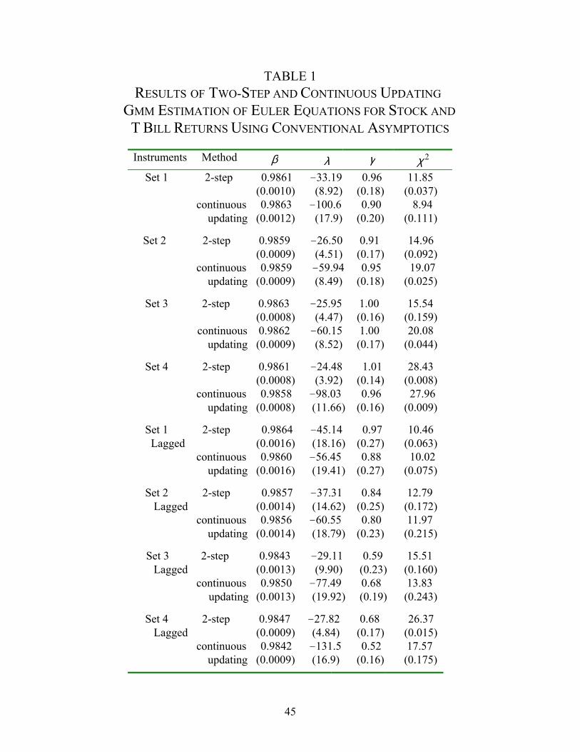
TABLE 1 RESULTS OF TWO-STEP AND CONTINUOUS UPDATING GMM ESTIMATION OF EULER EQUATIONS FOR STOCK AND T BILL RETURNS USING CONVENTIONAL ASYMPTOTICS

Instruments Method β λ γ 2χ Set 1 2-step 0.9861 -33.19 0.96 11.85 (0.0010) (8.92) (0.18) (0.037) continuous 0.9863 -100.6 0.90 8.94 updating (0.0012) (17.9) (0.20) (0.111)

Set 2 2-step 0.9859 -26.50 0.91 14.96 (0.0009) (4.51) (0.17) (0.092) continuous 0.9859 -59.94 0.95 19.07 updating (0.0009) (8.49) (0.18) (0.025)

Set 3 2-step 0.9863 -25.95 1.00 15.54 (0.0008) (4.47) (0.16) (0.159)

continuous 0.9862 -60.15 1.00 20.08 updating (0.0009) (8.52) (0.17) (0.044)

Set 4 2-step 0.9861 -24.48 1.01 28.43 (0.0008) (3.92) (0.14) (0.008) continuous 0.9858 -98.03 0.96 27.96 updating (0.0008) (11.66) (0.16) (0.009) Set 1 2-step 0.9864 -45.14 0.97 10.46 Lagged (0.0016) (18.16) (0.27) (0.063) continuous 0.9860 -56.45 0.88 10.02 updating (0.0016) (19.41) (0.27) (0.075)

Set 2 2-step 0.9857 -37.31 0.84 12.79 Lagged (0.0014) (14.62) (0.25) (0.172) continuous 0.9856 -60.55 0.80 11.97 updating (0.0014) (18.79) (0.23) (0.215)

Set 3 2-step 0.9843 -29.11 0.59 15.51 Lagged (0.0013) (9.90) (0.23) (0.160) continuous 0.9850 -77.49 0.68 13.83 updating (0.0013) (19.92) (0.19) (0.243)

Set 4 2-step 0.9847 -27.82 0.68 26.37 Lagged (0.0009) (4.84) (0.17) (0.015) continuous 0.9842 -131.5 0.52 17.57 updating (0.0009) (16.9) (0.16) (0.175)

45

(continued from Table 1 on the last page)

Note.-Set 1 includes four instruments: 1, and first lags of consumption growth,

term premium, and real dividend yield. Set 2 includes Set 1 and the first lags of real T Bill rate and labor income growth. Set 3 is Set 2 and the first lag of the default premium. Set 4 is Set 3 and Lettau and Ludvigson (2004)’s cay. Standard errors are in parentheses, except for the last column, which reports the minimum

test of over-identifying restrictions and the corresponding p-values in

parentheses. The degree of freedom for the test is the number of orthogonality conditions (i.e. the number of instruments×2) subtracted by 3, the number of parameters estimated.

2χ2χ

46

TABLE 2 PARAMETER VALUE RANGES AND INCREMENTS

IN S SET ANALYSIS

β λ γ Range [0.983, 1.01] [-150, 2] [0.401, 2.521] Increment 0.001 0.25 0.02

Note.-The range of β only affects the joint S set for all the three parameters.

47

TABLE 3 RESULTS OF S SET ANALYSIS OF THE EULER EQUATIONS (10) FOR

STOCK AND TREASURY BILL RETURNS

Instruments 95% Joint S Set for ( β , λ ,γ ) β λ γ RRA EIS

Set 1 Set 1 Lagged

[0.984, 0.988] [-150, -17.25] [0.401, 1.041] [0.0025, 90.85] [0.961, 2.494] [0.983, 0.987] [-150, -10.25] [0.401, 1.081] [0.0025, 90.85] [0.925, 2.494]

Set 2 [0.985, 0.986] [-87.25, -37.5] [0.73, 1.01] [0.17, 19.94] [0.99, 1.37] Set 2 Lagged [0.983, 0.988] [-150, -3.75] [0.401, 1.221] [0.002, 74.5] [0.819, 2.49]

Set 4 Null Set 4 Lagged [0.983, 0.987] [-150, -46.25] [0.401, 1.001] [0.85, 90.85] [0.999, 2.49]

95% Concentrated S Set for ( λ ,γ ) 95% Concentrated S Set for λ λ γ RRA EIS λ RRA EIS

Set 1 Set 1 Lagged

[-150, -26.25] [0.401, 1.021] [0.0025, 90.85] [0.979, 2.494] [-150, -15.75] [0.401, 1.041] [0.0025, 90.85] [0.961, 2.494]

[-107.75, -48] [4.18, 13.66] [1.067, 1.13] [-110.5, -48] [6.28, 27.83] [1.123, 1.32]

Set 2 Set 2 Lagged

[-74, -47.25] [0.841, 1.001] [0.93, 11.8] [0.999, 1.189] [-150, -15] [0.401, 1.061] [0.0025, 84.86] [0.943, 2.494]

Null [-150, -20.25] [1.68, 77.28] [1.035, 2.43]

Set 4 Set 4 Lagged

Null [-150, -52.25] [0.401, 1.001] [0.85, 91] [0.999, 2.494]

Null [-150, -58.75] [26.2, 74.5] [1.75, 1.96]

Note.―This table presents the ranges of each parameter in a 95% S set and the ranges of implied RRA and EIS values. These ranges are, however, not the 95% confidence intervals for individual parameters. The results when instrument set 3 is used are similar to those for instrument set 2 and are not reported to conserve space.

48

TABLE 4 SELECTED ELEMENTS OF 95% S SETS, IMPLIED VALUES OF RRA AND

EIS, QUARTERLY EQUITY PREMIUM, AND RISKFREE RATE

β λ γ RRA EIS E.P. fr Joint S Set for ( β , λ , γ ), Instrument Set 1

0.9866 -51.25 0.981 1.974 1.019 0.0149 0.0045 0.9867 -51.25 1.001 0.949 0.999 0.0149 0.0044 0.9866 -51.50 0.981 1.979 1.019 0.0150 0.0047 0.9868 -51.75 1.001 0.948 0.999 0.0150 0.0046

Joint S Set for ( β , λ , γ ), Instrument Set 2

0.9865 -48.75 0.971 2.414 1.030 0.0141 0.0046 0.9866 -48.75 0.991 1.439 1.009 0.0140 0.0045 0.9865 -49.00 0.971 2.421 1.030 0.0142 0.0042 0.9866 -49.00 0.991 1.441 1.009 0.0141 0.0041

Joint S Set for ( β , λ , γ ), Instrument Set 3 0.9867 -51.50 1.001 0.949 0.999 0.0149 0.0045 0.9866 -51.50 0.981 1.979 1.019 0.0150 0.0047 0.9868 -51.75 1.001 0.948 0.999 0.0150 0.0046 0.9867 -52.00 0.981 1.988 1.019 0.0152 0.0043

Concentrated S Set for ( λ ,γ ), Instrument Set 1 ─ -51.25 0.981 1.978 1.019 0.0149 ─ ─ -51.50 0.981 1.979 1.019 0.0150 ─ ─ -51.75 0.981 1.983 1.019 0.0151 ─

Concentrated S Set for ( λ ,γ ), Instrument Set 2 ─ -51.50 1.001 0.949 0.999 0.0149 ─ ─ -51.50 0.981 2.002 1.019 0.0150 ─ ─ -51.75 0.981 1.983 1.019 0.0151 ─

Concentrated S Set for ( λ ,γ ), Instrument Set 3

─ -51.50 0.981 1.979 1.019 0.0150 ─ ─ -51.75 0.981 1.983 1.019 0.0151 ─ ─ -51.75 1.001 0.948 0.999 0.0150 ─

Note.─The first three columns report selected elements in the 95% joint S sets or concentrated S sets. The next two columns present the implied RRA and EIS values implied by the λ and γ values of each row. The column labeled “E.P.” shows the unconditional quarterly equity premium implied by the values of RRA and EIS in each row under the assumption of lognormality for consumption growth and asset returns. The last column reports the quarterly risk-free rate implied by the values of β , λ , γ of each row in the upper panel.

49

TABLE 5 FEASIBILITY CONDITION AND TRANSVERSALITY CONDITION β δ EIS RRA Feasibility Transversality Joint S Set for ( β , λ , γ ), Instrument Set 1 0.9866 0.01358 1.019 1.974 0.0137 -0.0225 0.9866 0.01358 1.019 1.979 0.0137 -0.0226 0.9867 0.01348 0.999 0.949 0.0135 -0.0224 0.9868 0.01338 0.999 0.948 0.0134 -0.0222 Joint S Set for ( β , λ , γ ), Instrument Set 2 0.9865 0.01368 1.030 2.414 0.0139 -0.0228 0.9865 0.01368 1.030 2.421 0.0139 -0.0228 0.9866 0.01358 1.009 1.439 0.0137 -0.0225 0.9866 0.01358 1.009 1.441 0.0137 -0.0225 Joint S Set for ( β , λ , γ ), Instrument Set 3 0.9866 0.01358 1.019 1.979 0.0137 -0.0226 0.9867 0.01348 0.999 0.949 0.0135 -0.0224 0.9867 0.01348 1.019 1.988 0.0136 -0.0224

0.9868 0.01338 0.999 0.948 0.0134 -0.0221

Note.─This table demonstrates that the joint S set elements in Table 4 that simultaneously match the equity premium and the riskfree rate satisfy the feasibility condition and the transversality condition in Smith (1996) for the EZW model.

50

TABLE 6 RESULTS OF S SET ANALYSIS OF THE CONSUMPTION EULER EQUATION

Instruments 95% Joint S Set for ( β , λ ,γ )

β λ γ RRA EIS Set 5 [0.983, 0.988] [-100, 2] [0.401, 1.541] [0.0018, 60.9] [0.649, 2.494]

Set 5 Lagged [0.983, 0.992] [-100, 2] [0.401, 2.261] [0.0018, 60.9] [0.442, 2.494] 95% Concentrated S Set for ( λ ,γ ) 95% Concentrated S Set for λ

λ γ RRA EIS λ RRA EIS Set 5

Set 5 Lagged [-100, 2] [0.401, 1.361] [0.0018, 60.9] [0.735, 2.494] [-100, 2] [0.401, 2.101] [0.0018, 60.9] [0.476, 2.494]

-86.0 and –93.0 1.812 and 6.738 1.009 and 1.072 0.75 0.972 1.039

Note.―The instrument set 5 includes 1, the first and second lags of real consumption growth, the first lag of household net worth growth, and the first lags of the real after-tax labor income growth, the term premium, the real dividend yield, and the default premium.

51

0.6

0.7

0.8

0.9

1

1.1

1.2

1.3

1959

.2

1960

.3

1961

.4

1963

.1

1964

.2

1965

.3

1966

.4

1968

.1

1969

.2

1970

.3

1971

.4

1973

.1

1974

.2

1975

.3

1976

.4

1978

.1

1979

.2

1980

.3

1981

.4

1983

.1

1984

.2

1985

.3

1986

.4

1988

.1

1989

.2

1990

.3

1991

.4

1993

.1

1994

.2

1995

.3

1996

.4

1998

.1

1999

.2

2000

.3

2001

.4

Year.Quarter

Gro

ss R

etur

n

Fig. 1.—The real value-weighted return of NYSE stocks (dashed line) and , the real return on optimal portfolio incorporating human capital (solid line). Both are quarterly rates.

mtR 1+

52

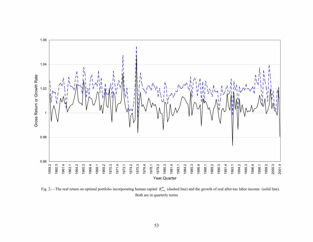
0.96

0.98

1

1.02

1.04

1.06

1959

.2

1960

.3

1961

.4

1963

.1

1964

.2

1965

.3

1966

.4

1968

.1

1969

.2

1970

.3

1971

.4

1973

.1

1974

.2

1975

.3

1976

.4

1978

.1

1979

.2

1980

.3

1981

.4

1983

.1

1984

.2

1985

.3

1986

.4

1988

.1

1989

.2

1990

.3

1991

.4

1993

.1

1994

.2

1995

.3

1996

.4

1998

.1

1999

.2

2000

.3

2001

.4

Year.Quarter

Gro

ss R

etur

n or

Gro

wth

Rat

e

Fig. 2.—The real return on optimal portfolio incorporating human capital (dashed line) and the growth of real after-tax labor income (solid line).

Both are in quarterly terms

mtR 1+

53

(a)

(c)

(b)

(d) (Fig. 3 to be continued)

54

(Fig. 3 continued from last page)

(e)

(g)

(f) Fig. 3. —The 95% Concentrated S Set (Shaded) for λ and γ and the 95% Confidence Ellipse for the 2-Step GMM Estimates of λ and γ Based on (a). Instrument Set 1; (b). Instrument Set 1 Lagged; (c). Instrument Set 2; (d). Instrument Set 2 Lagged; (e). Instrument Set 3; (f). Instrument Set 3 Lagged; and (g). Instrument Set 4 Lagged.

55