CITYPERC Working

Paper Series

no. 2013/04

CITYPERC

City Political Economy Research Centre

Department of International Politics

City University London

Northampton Square

London EC1V 0HB

ISSN 2051-9427 Contact: cityperc@city.ac.uk

1

Do Politicians Serve the One Percent?

Evidence in OECD Countries.

Pablo Torija1

Abstract

Present social movements, as “Occupy Wall Street” or the Spanish “Indignados”, claim

that politicians work for an economic elite, the 1%, that drives the world economic policies.

In this paper we show through econometric analysis that these movements are accurate:

politicians in OECD countries maximize the happiness of the economic elite. In 2009

center-right parties maximized the happiness of the 100th-98th richest percentile and

center-left parties the 100th-95th richest percentile. The situation has evolved from the

seventies when politicians represented, approximately, the median voter.

Keywords: Democracy, representation, economic elite, political economy, Occupy Wall-Street.

1 University of Padova.

2

INTRODUCTION:

The financial crisis which had broke out in the USA in 2007 turned into a world wide

economic disaster by 2008. That year, thousands of citizens from Greece, Portugal and

Iceland expressed their anger against politicians and their economic management. Three

years later, and with the Arab spring in between, around 7 millions of Spanish “indignados”

started a massive demonstration campaign. By September 2011, the outrage against

politicians had already crossed the Atlantic and the “Occupy Wall-Street” movement

claimed for a refunding of the economic and political system in the USA.

Civil society from all OECD countries participated in a world-wide coordinated

demonstration on 15th October 2011. Their activists claimed that they are not enjoying real

democratic systems. They complained that politicians do not follow the wishes of the

majority but the dictates of an economic elite, and considered that their politicians were

excluding the remaining 99% of the population.

These movements are inspired by the work of several researchers (eg. Sirorta

2007, Taibbi 2010, George 2011, or Stiglitzt 2011) who suggest that political parties in

developed societies are not any longer a fair representation of the citizens' wills but an

instrument of the rich. For instance, Colin Crouch claims in his book 'Post-democracy'

(Crouch, 2004) that developed countries enjoy only pseudo-democratic regimes as they

lack truly representative elections. Crouch considers that this evolution is due the relative

impoverishment of the workforce and labor unions after the seventies as a main cause of

this situation. Another researcher Slavov Žižek, suggests that ecological disasters are not

the only occurrences that may be used to impose the rule of the economic elite, as

theorized by Naomi Klein (Klein 2007). The economic crisis itself can be instrumented to

set economic rules which favor the interests of the richest (Žižek 2009).

Economic journals are full with papers which explain how interest groups can take

advantages of a large variety of undemocratic channels. Democratic deficits are linked

with the action of lobbies (Fellini and Merlo 2003, or Baldwin and Robert-Nicoud, 2007.),

media (Prat and Strömberg, 2011 or Edmond, 2011), public prosecution (Alt and Lassen,

2010 or Torija 2011), rent extraction (Dreher and Schneider, 2010. or Ferraz and Finan,

2011.), etc... Researches who have studied these aspects in depth found out that many of

them directly affect OECD democracies.

On the other hand, several important research institutes share a totally different

view. Freedom House (FH), National Center of Competence in Research (NNCR), Centre

3

for Systemic Peace (CSP), and the Worldwide Governance Indicators project (WGI) create

annual indexes and reports about the democratic quality of the developed world. All their

indexes use several panels of experts and statistical data, and they coincide on the

strength and robustness of the democratic systems in all OECD countries.

For instance, according to FH “it is unlikely that Europe’s democratic standards will

suffer serious setbacks in the wake of the ongoing debt crisis” (Freedom House 2012).

NNCR similarly concludes in one of its reports: “Contrary to the contemporary political

discourse, the results show that there is no evidence of an overall crisis or a decline in the

quality of democracy” (Bühlmann, M. et al, 2011). From a quantitative point of view, they

show an improvement in the quality of democratic representation of OECD countries

during the period 1990 -2007.

Another index which has quantified the quality of developed democracies for a long

period is Polit IV from CSP. The index has a 20 point scale and it has continually increased

for OECD countries from 1981 till 2009, with the exception of Belgium that lost two points

due to problems in forming a government. Finally, WGI finds slight decreases in both

“Voice and Accounting” and “Goverment Effectivenes” indexes for the period 1996-2009 in

OECD countries, but these reductions are statistically insignificant (Kaufmann, Kraay and

Mastruzzi, 2009).

These examples illustrate the important divergences between several institutes,

authors and citizens when talking about the quality of democracy. This paper aims to be a

contribution to the debate.

Concretely, the paper will try to describe the level of representation of developed

democracies and analyze the validity of the theories of Collin Crouch. The paper will study

whether parties in government satisfy the desires of the majority of the society or if they

focus on the interest of the rich. It shows the evolution of the political representation and it

also discusses the correlations between the level of representation and the power of the

working-class.

To do so, we will combine the information about happiness and income of

individuals from the World Values Survey (World Values Survey 2009) and the The

Mannheim Eurobarometer Trend File 1970-1999 (Schmitt. 2001) with the Potrafke's

ideology index, which shows the ideology of a given government in a particular country

(Potrafke, 2009). The final database covers 1981 to 2009 and uses more than 160,000

surveys on 24 rich OECD countries. Through econometric analysis, we can analyze how

the interests of particular citizens are fulfilled by politicians. We will show how the policies

4

implemented by different governments evolved and how they maximize the happiness of

the economic elite in 2009. Through extrapolation we can show also how politicians

represented the median voter around the seventies.

The paper is organized as follows. First, we explain the theory of post-democracy

and we synthesize the ideas of Acemoglu and Robinson (2006) who modeled it in

economic terms. In section 2, we describe the econometric model, its characteristics and

the variables used. The results are presented in section 3 and they are discussed in

section 4. At the end, we include a conclusion section that summarizes the paper.

SECTION 1: THEORY

1.1 Post-democracy

Collin Crouch summarized in his book “Post-democracy” several years of research

in Northern democracies. According to the author, the power of the working-class in rich

countries has evolved in a parabolic way. After the Second World War their power was in a

minimum, but workers started to gain power and representation during two or three

decades reaching their peak in the seventies. By that time, they had managed to bring

their political agendas to different governments. Those governments implemented

Keynesian policies which robust the access of workers to public and private goods. The

situation started to change in the seventies when the companies displaced the activities of

manual workers to the periphery. Little by little, all governments shifted their policies to

favor large transnational corporations. The labor unions were weakened and the power of

workers declined.

The quality of democratic representation also evolved in a parabolic trajectory. In

the seventies, different parties favored different individuals according to the party's

ideological background, but this situation changed later. According to the author,

politicians only represent the economic elite now-a-days. Therefore. elections certainly

occur in rich countries but they lack real representation.

1.2 Modeling post-democracy

Acemoglu and Robinson wrote in their paper “Persistence of powers, elites and

institutions” (Acemoglu and Robinson 2006), a mathematical model which fits with the

theory exposed by Crouch. We will try to summarize the intuition behind this paper:

In their model there is a large number of worker-citizens and smaller group of elite-

individuals. Both groups compete to establish economic institutions which might favor one

5

group or the other. The authors analyze the existence of a “captured democracy”, when

democratic institutions are created but the economic elite is able to monitor them and

impose their favorite set of economic institutions. Whether the elite is able to capture the

democratic process is a bargaining process between their power, PE, and the power of the

worker-citizens, PC. In their model the power of the elite is a positive function of the rents

that they extract from the total national rent PE = f(R/Y) and the power of the workers is a

positive function of their contributions to obtain political power PC = f(θ). The democratic

institutions would favor the economic elite when PE >> PC.

As we see, there are many similarities between this model and the ideas presented

by Crouch: The possibility of existing unrepresentative democracies and the role of the

power of the working-class. Both studies propose an interesting empirical question: the

existence of political institutions which benefit the economic elite is correlated with the

rents of this elite and the contributions of workers to the bargaining power.

Although Acemoglu and Robinson do not use their model to analyze the situation of

rich countries, we will use their theoretical framework for empirical research in OECD

countries. Namely, we will consider the percentage of national rents as wages and the

percentage of workers in labor unions to measure the political power of elite and the

contributions of workers to the political bargain. We will analyze whether these variables

are correlated with the quality of representation in OECD democracies.

SECTION 2: METHODOLOGY

2.1 Estimation of political representation

The first step is to measure the quality of political representation. We will try to

quantify the income level of the individual which different political parties are representing.

Whether she is a rich individual, the median individual or a poor individual. The

econometric regression is inspired in the traditional downsian model (Downs, 1957). Using

the notation of Patty, Snyder, and Ting (2008):

Let be K political parties that must choose a policy xk which they will implement if

they are in power. xk is characterized in the set of real numbers X.

There is a number N of i voters. Each voter has an income yi and a favorite policy,

τi, related to this income. The function h identifies this relation, h(yi ) = τi . The set of τi is Τ =

X.

6

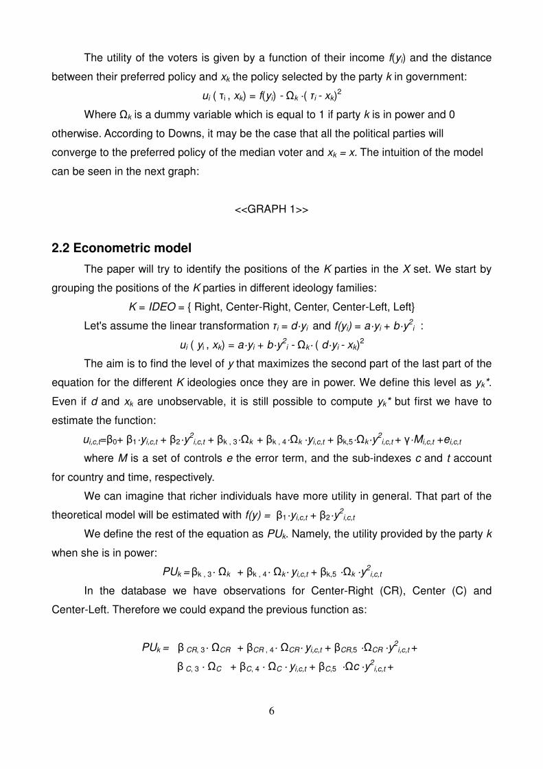
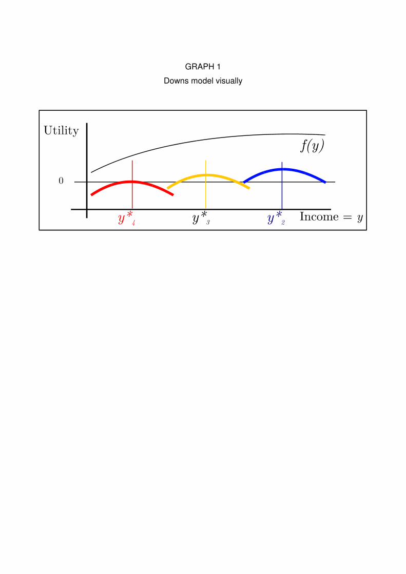
The utility of the voters is given by a function of their income f(yi) and the distance

between their preferred policy and xk the policy selected by the party k in government:

ui ( τi , xk) = f(yi) - Ωk ·( τi - xk)2

Where Ωk is a dummy variable which is equal to 1 if party k is in power and 0

otherwise. According to Downs, it may be the case that all the political parties will

converge to the preferred policy of the median voter and xk = x. The intuition of the model

can be seen in the next graph:

<<GRAPH 1>>

2.2 Econometric model

The paper will try to identify the positions of the K parties in the X set. We start by

grouping the positions of the K parties in different ideology families:

K = IDEO = Right, Center-Right, Center, Center-Left, Left

Let's assume the linear transformation τi = d·yi and f(yi) = a·yi + b·y2i :

ui ( yi , xk) = a·yi + b·y2i - Ωk· ( d·yi - xk)

2

The aim is to find the level of y that maximizes the second part of the last part of the

equation for the different K ideologies once they are in power. We define this level as yk*.

Even if d and xk are unobservable, it is still possible to compute yk* but first we have to

estimate the function:

ui,c,t=β0+ β1·yi,c,t + β2·y2i,c,t + βk , 3·Ωk + βk , 4·Ωk ·yi,c,t + βk,5·Ωk·y

2i,c,t + γ·Mi,c,t +ei,c,t

where M is a set of controls e the error term, and the sub-indexes c and t account

for country and time, respectively.

We can imagine that richer individuals have more utility in general. That part of the

theoretical model will be estimated with f(y) = β1·yi,c,t + β2·y2i,c,t

We define the rest of the equation as PUk. Namely, the utility provided by the party k

when she is in power:

PUk = βk , 3· Ωk + βk , 4· Ωk· yi,c,t + βk,5 ·Ωk ·y2i,c,t

In the database we have observations for Center-Right (CR), Center (C) and

Center-Left. Therefore we could expand the previous function as:

PUk = β CR, 3· ΩCR + βCR , 4· ΩCR· yi,c,t + βCR,5 ·ΩCR ·y2i,c,t +

β C, 3 · ΩC + βC, 4 · ΩC · yi,c,t + βC,5 ·Ωc ·y2i,c,t +

7

β CL, 3· ΩCL + βCL , 4· ΩCL· yi,c,t + βCL,5 ·ΩCL ·y2i,c,t +

then, we can find the level of income that maximize each k = CR, C, CL political

party by applying the first order condition to PUk :

yk*: ∂ PUk / ∂ y = 0

yk* = - βk , 4 / ( 2 · βk , 5)

In this way we could identify the different yk*, which is the aim of the paper.

Unfortunately, this procedure generates serious problems with the brant-test (see Section

2.4) and alternatives must be considered.

Concretely, to overcome this problem we have assigned numeric values for the

different K ideologies. We have created a new variable called ideo, which is equal to one if

Right parties are in government, two if Center-Right parties are in government, etc:

ideo = 1,2,3,4,5

We have restated the previous model as:

ui ( yi , xk) = a·yi + b·y2i - ( ideo + ideo2) ·( d·yi - xk)

2

and we can estimate it:

ui,c,t= β0 + β1·yi,c,t+β2·y2i,c,t+ β 3·ideoct+β 4·ideo2

ct+β5·ideoct yi,c,t+β6·ideoct·y2i,c,t + β7

·ideo2ct·yi,c,t +γ·Mi,c,t +ei,c,t

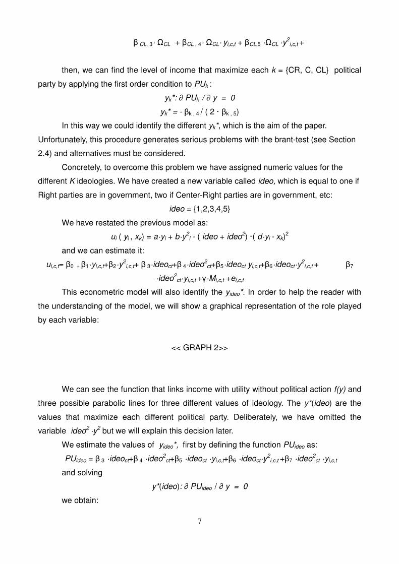
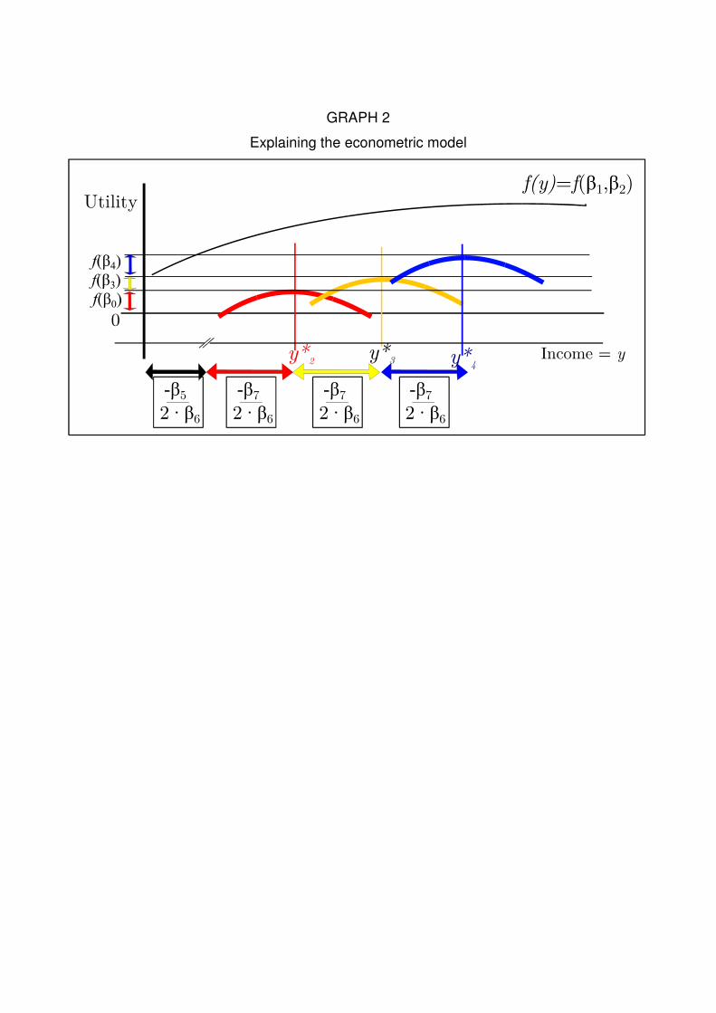
This econometric model will also identify the yideo*. In order to help the reader with

the understanding of the model, we will show a graphical representation of the role played

by each variable:

<< GRAPH 2>>

We can see the function that links income with utility without political action f(y) and

three possible parabolic lines for three different values of ideology. The y*(ideo) are the

values that maximize each different political party. Deliberately, we have omitted the

variable ideo2 ·y2 but we will explain this decision later.

We estimate the values of yideo*, first by defining the function PUideo as:

PUideo = β 3 ·ideoct+β 4 ·ideo2ct+β5 ·ideoct ·yi,c,t+β6 ·ideoct·y

2i,c,t +β7 ·ideo2

ct ·yi,c,t

and solving

y*(ideo): ∂ PUideo / ∂ y = 0

we obtain:

8

y*(ideo)= - (β 5+ β 7 ·ideo )/ ( 2 · β6)

There are two important notes to this formulation. First, the inclusion of the variable

ideo2 in ui ( yi , xk) = a·yi + b·y2i - ( ideo + ideo2) ·( d·yi - xk)

2 is necessary in order to obtain

different peaks for different ideologies. And second, it is important to notice that here the

distance y*(ideo) - y*(ideo+1) = β 7 is constant for all values of ideo. We have called this

assumption the symmetry-assumption and we have discussed it in detail later on.

Obviously, if β7 = 0, then y*(ideo) = y*

We can extend the empirical model to analyze how y* evolves across time, and due

to the effect of other variables. Given:

F(y, ideo)=β1·yi,c,t+β2·y2i,c,t+ β 3·ideoct+β 4·ideo2

ct+β5·ideoct yi,c,t+β6·ideoct·y2i,c,t

+β7·ideo2ct·yi,c,t

We will calculate:

ui,c,t= F(y, ideo) + δ·ti,c,t ·ideoct·yi,c,t + η·P·ideoct·yi,c,t+γ·Mi,c,t +ei,c,t

where: t is a year variable. P is a vector with values for the macro-economic

variables of interest: The percentage of national rent paid as wages (wagessh), and

participation in labor unions (labor).

We have also added other control variables that interact simultaneously with

ideology and income, namely: Gini index (gini), GDP per capita (gdp), unemployment

(unemp), turnout in the last elections (turnout), economic growth (growth), percentage of

population with colleague education (unieduc). M will include the interactions between

variables t and P with ideo and income.

The new y* are defined by:

y*(ideo)= - (β 5+ β 7 ·ideoc,t +δ·ti,c,t + η·P ) / ( 2·β6)

Now, time (t) and the set of macro-economic variables (P) determine also the

platform of the different parties when they are in government.

2.3 Independent Variables

The period of study goes from 1981 till 2009. There is a total of 24 OECD countries

analyzed. Some countries have been surveyed twice and present around 2.000

observations (eg. New Zealand), and some of them have been surveyed ten times (eg.

Great Britain). It is possible to find a list of years and when where they surveyed in the

appendixes (APPENDIX 1).

Income is a key variable which is measured with different scales in both databases.

9

The most recurrent way of measuring income in both databases was using an 11-steps

scale. Therefore, we have converted all the other scales to fit the 11-steps scale. If a given

scale had N steps we have divided each n step between N and we have multiplied the

result by 11. The final scale for the income variable is therefore in the interval (0,11]

Government ideology is measured with the Potrafke's ideology index. It is described

as follows:

“This index places the cabinet on a left-right scale with values between 1 and

5. It takes the value 1 if the share of governing right wing parties in terms of

seats in the cabinet and in parliament is larger than 2/3, and 2 if it is between

1/3 and 2/3. The index is 3 if the share of center parties is 50%, or if the left

wing and right wing parties form a coalition government that is not dominated

by one side or the other. The index is symmetric and takes the values 4 and 5

if the left wing parties dominate.” (Potrafke, 2009).

The databases do not have observations on the most extreme cases, 1 and 5. Only

the values 2, 3 and 4 are present in the final data analyzed.

Other macro economic variables belonging to the vector P comes from the

databases of World Bank, Eurostat and OECD.

The final analysis has +100.000 interviews for those regressions that consider only

the World Values Survey (WVS) and +160.000 for those which use WVS with Schmitt 2011

in a merged database. A detailed summary of the variables can be found in the

appendixes (APPENDIX 2).

2.4 Dependent variable: Level of Happiness.

There is a large literature dealing with the concept of utility and how to measure it.

In the last decade psychologists and sociologist have proposed certain ways of obtaining a

self-reported level of utility (Frey and Stutzer, 2002). There are two ways of measure

indirectly utility, one is to ask people for their level of “happiness” and the other to ask for

their level of “satisfaction with life”.

Many authors presuppose that both measurements are identical (Gundelach and

Kreiner, 2004). Others claim that the level of happiness is the correct way of measuring

utility (Lane 2000), and consider satisfaction as the distance between aspirations and

achievements (Campbell et al. 1976). The distance between aspirations and achievements

may depend on the policies of former governments, and we are trying to estimate the

10

political position of present governments. Additionally, the number of observations

containing the answer to the question about happiness are 50% more than the those

containing the answer to the question about the level of satisfaction. Consequently, we

consider the level of happiness as dependent variable. Therefore, the different values of y*

represent the happiness of which individuals are maximizing the politicians.

There are some problems when we use happiness as a dependent variable.

Happiness is an emotional state which depends in several factors ranging from weather to

health. The capacities of a government to influence happiness are limited but, as we will

show, there is an impact of the political decisions of governments on the happiness of their

citizens.

The level of happiness and other micro-level data are collected from World Values

Survey (2009) and The Mannheim Eurobarometer Trend File 1970-1999 (Schmitt. 2001).

The latest only includes information about individual's happiness for EU countries during

the period 1981-1986. This may create a selection-bias problem and we have to take the

results that includes the Eurobarometer with caution.

Additionally, both databases are not completely identical and we had to carry some

transformations. For instance both databases ask for the level of happiness. Respondents

could choose four different answers in the WVS: “Very happy”, “Quiet Happy”, “Not very

happy”, “Not happy at all” and only three in Schmitt (2001) “Very happy”, “Happy”, “Not

happy”. Table 1, shows the distribution of these answers.

<<Table 1>>

In order to handle this discrepancy we have carried out two sets of regressions. The

first one only with the observations of the WVS, which measures happiness with has a 4-

steps scale. The other one, combines WVS and Schmitt (2001). It considers “Not very

happy” and “Not happy at all” from WVS as the answer “Not happy” in Schmitt (2001),

therefore it measures happiness with a 3-steps scale.

Moreover, there are several problems related with the use of self-reported

happiness. Concretely, World Values Survey asks: “Taking all things together, would you

say you are:”. We can name the possible set of answers as J:

J = “Very happy”, “Quiet Happy”, “Not very happy”, “Not happy at all”.

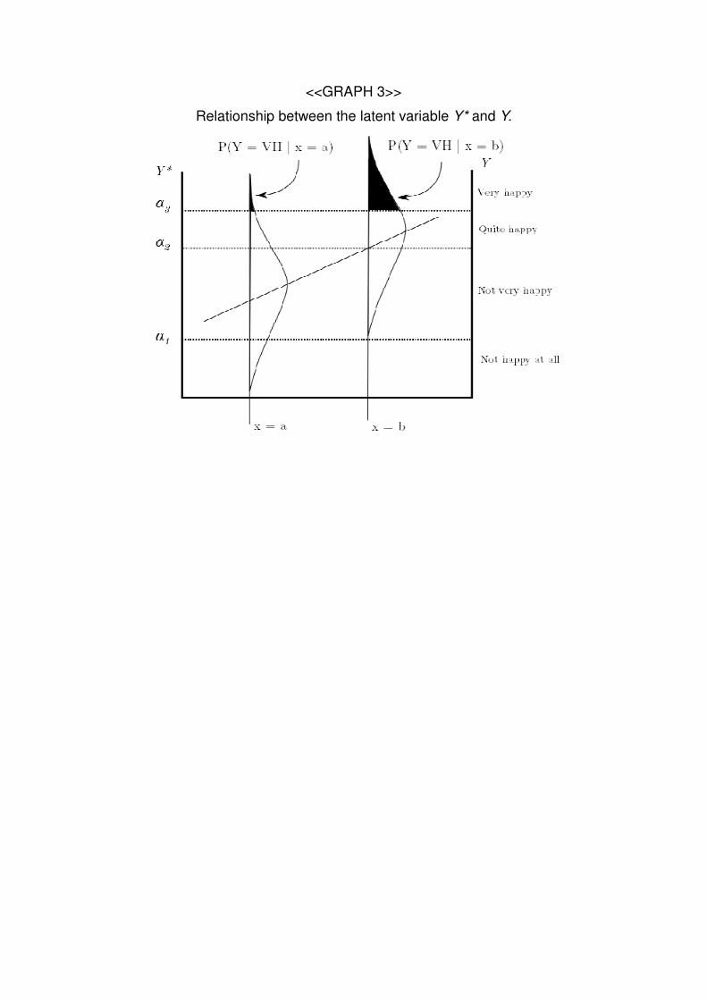
As the possible answers lack cardinality, it is necessary to treat them with ordinal

models. The standard procedure is to calculate J -1 ordinary binomial models.:

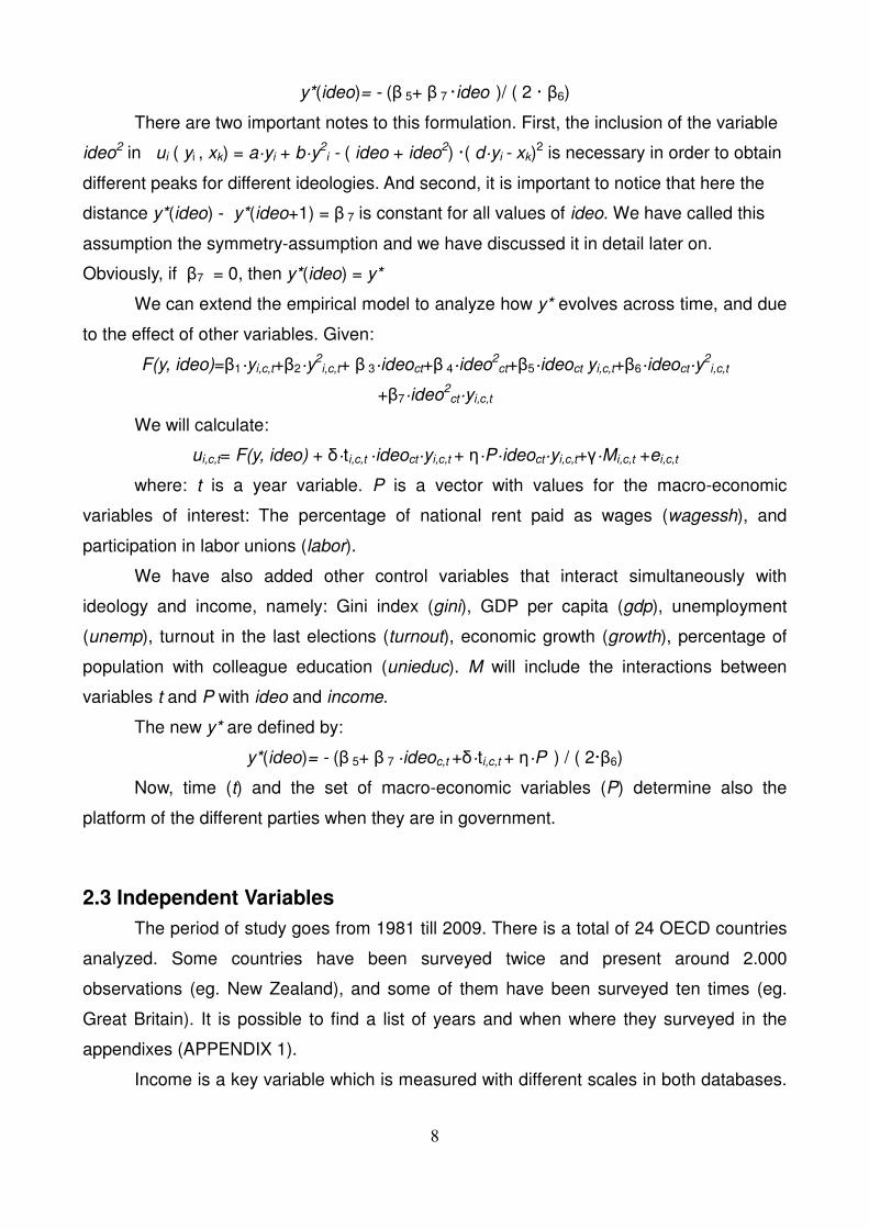
logit [P (Y ≤ j |x)] = αj + β j 'x j = 1 … J-1

If βj =β for all j, then we will have a continuous latent variable underlining Y (Agresti,

11

2000). We can denote that variable as Y*. We show the relation between Y and Y* in

Graph 3 (adapted from Agresti, 2000.)

<<GRAPH 3>>

Obviously, only continuous variables can be derived. Therefore, βj =β is a necessary

condition of the econometric model. We can test whether βj =β by implementing a Brant

test (Brant, 1990). This requirement supposes, obviously, a strong limitation to the

research.

The procedure to obtain an unbiased and differentiable set of variables has been

the following: First we carried out an ordinal logistic regression, then we have performed

the Brant test (Long and Freese 2001) and finally, in case of rejecting the null hypothesis

of non-parallel lines, we have performed a ordinal general logit model with the weights and

heteroskedasticity function indicated in the appendixes (APPENDIX 3).

2.5 Regressions

The result table shows six different regressions. They are labeled as BASIC-4,

BASIC-3, YEAR-4, YEAR-3 , NOCO-4 COMP-4.

In the BASIC regressions, y* are fixed. YEAR regressions include the variable

year·income·ideo that allows for changes of y* over time. The NOCO regression calculates

the influence of labor union affiliation (labor·income·ideo) and percentage of rents payed

as wages (wagessh·income·ideo) with y*. It does not include other variable interacting with

income·ideo which may work as controls. The COMP regression computes the interactions

between y* with time and the complete vector of macro-variables P = (gini), (gdp),

(unemp), (turnout), (growth), (unieduc). The numeric suffixes (ie. 3,4) indicate the

number of steps of happiness, the dependent variable.

Problems related with the parallel-line assumption arise when including all the

controls. BASIC, and YEAR regressions do not have all of them, but the controls

eliminated were all insignificant. These eliminated controls are: unieduc, and the

interactions, unieduc·ideo, unieduc·income, labor·income and gini·income. In the

appendixes (APPENDIX 3) it is possible to find the large list of controls used.

On the other hand, NOCO-4 and COMP-4 do not hold the parallel-line assumption

for some key coefficients. The result table indicates which are those coefficients.

Finally, all the regressions have the same weighting and clustering specifications to

12

obtain unbiased results and accurate errors. It is possible these characteristics in the

appendixes (APPENDIX 3).

SECTION 3: RESULTS

In this section, we present the regressions previously described, and a preliminary

analysis of the results obtained. Here, we will just show which variables determine the

position of y*, indicating their coefficients, z-values and whether they violate the parallel-

line assumption. We will denote y as “income”, its interaction with the ideology index as

“income·ideo”, the interaction of income, ideology index and year variables as

“year·income·ideo”, etc...

3.1 Result table

<<Table 2>>

3.2 Analysis

With the previous table it is possible to analyze the evolution of y* in the income

scale. Recall that we will compute the y* with:

y*(ideo)= - (β 5+ β 7 ·ideoc,t +δ·ti,c,t + η·P )/ ( 2·β6)

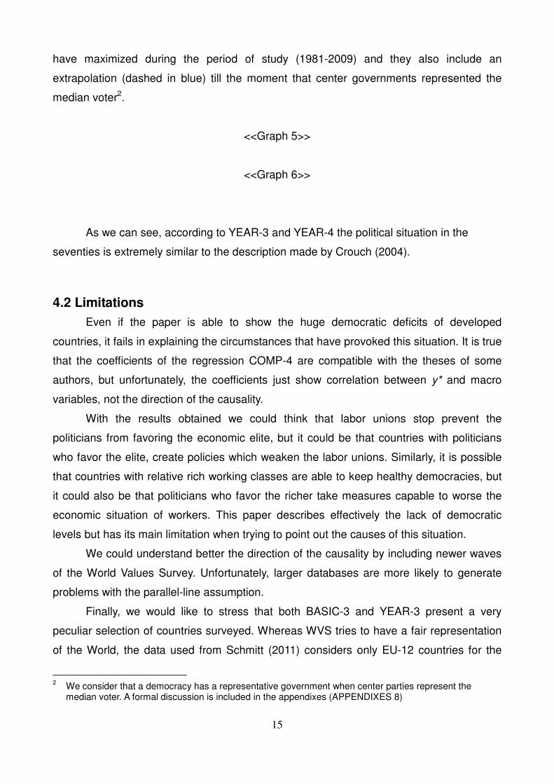
In general, a positive coefficient for δ or η will shift the y* to the left on the income

scale, towards the richer individuals, if t and P increase. For instance the coefficient of

year·income·ideo is greater than 0 meaning that every year the y* move to the left (i.e

politicians maximize the happiness of richer individuals continually). Remember that

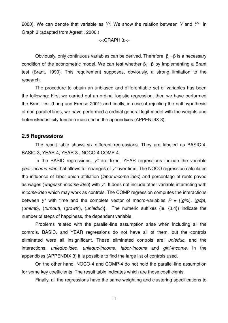
variable income was computed in an eleven step scale. We have parametrized the

distribution function of the variable income in order to extend the range to the infinite

(APPENDIXES 7). In order to help the reader with the interpretation of coming results, we

present here the distribution of income for BASIC-4, YEAR-4, NOCO.4 and COMP-4

<<GRAPH 4>>

This is the distribution function of the income-scale. For instance, when we mention

13

that the distance between Center-Left and Center-Rigt parties is 4,2 points, we should

imagine these distance in the horizontal axis of the previous graph. With this in mind we

can present here the results:

Result 1: There is not statistical difference on the individual that different political

parties represent once in power, although in some regressions this difference is large.

The variable income·ideo2 is insignificant in 4 out of 6 regressions. Only NOCON-4

and COMP-4 show a significant coefficient. In those regressions the coefficient does not

satisfy the parallel-line assumption, and we must take it with caution.

The other coefficients are statistically insignificant but in the case of the regressions

BASIC-4 and YEAR-4 they are large. The distances between y*'s in the different

regressions are shown in the next table.

<<Table 3>>

Result2: Politicians have maximized the happiness of richer individuals during the

period of study.

In both regressions the coefficient year·income·ideo is positive and significant. Each

model shows a different evolution of y*. Actually, the displacement is double for YEAR-4

than for YEAR-3.

<<Table 4>>

The difference may come due to the fact that the combined database (happiness in

3 steps) includes a large number of observations of Center Europe for the period 1981-

1986. According to several scholars those countries followed a different democratic

evolution than Japan, USA, Oceania or South Europe (Crouch 2004)

Result 3: Increases in the percentage of rents paid as wages and salaries, and the

level of affiliation to labor unions are correlated with governments that maximize the

happiness of poorer individuals.

We can calculate how an increase of 1% on the values of these variables shift the

position of y* for COMP-4. Countries where workers obtain a larger share of the national

rent and countries present governments that maximize the happiness of the poorer. 1% of

increase on these variables shifts more than one point the y* in the income scale . From

that perspective, changes on labor union affiliation are much moderated.

<<Table 5>>

We can also analyze how y* changes with changes of one standard deviation of the

14

variables of interest. In that case we see how the change in the share of wages is also

more important than the other.

SECTION 4: DISCUSSION.

4.1 Picturing democracy and representation.

Until this point we have described how politicians maximize the happiness of certain

y* individuals due to several factors. In this section we will illustrate the evolution of the

political representation over time. Concretely, how the y* for different parties over the

period of study. It is important not only to know the evolution in the income scale but also in

the income distribution function.

According to YEAR-3 and YEAR-4, politicians would maximize the happiness of the

following income percentiles at the beginning and at the end of the period of study.

<<Table 6>>

As we can see, since the eighties there has been a lack of political representation.

Furthermore, the data shows an extreme situation in 2009. Independently of the

regression used we see how all political parties in power maximized the happiness of the

richest individuals. In both regressions, we see how politicians maximize the happiness of

the 95th - 100th richest percentile.

This fact has already been denounced by many authors, who have tried to explain

the reasons of this evolution. Colin Crouch (2004) explained how the relative

impoverishment of workers, and the weakness of labor unions favored the rise of post-

democratic governments (ie. a government for and by the rich). The coefficients of

wagessh·income·ideo and labor·income·ideo may stand for this idea. These coefficients

show how societies with relative poorer workers (relative to capitalists) and weaker labor

unions coincide with politicians that maximize the happiness of richer individuals.

Crouch also explained how developed societies come closest to democracy in its

maximal sense after in the seventies. We cannot test this idea directly with the data as the

databases analyze the period 1981-2009. In any case, we can extrapolate backwards the

results obtained to the seventies to observe the positions of the different political parties.

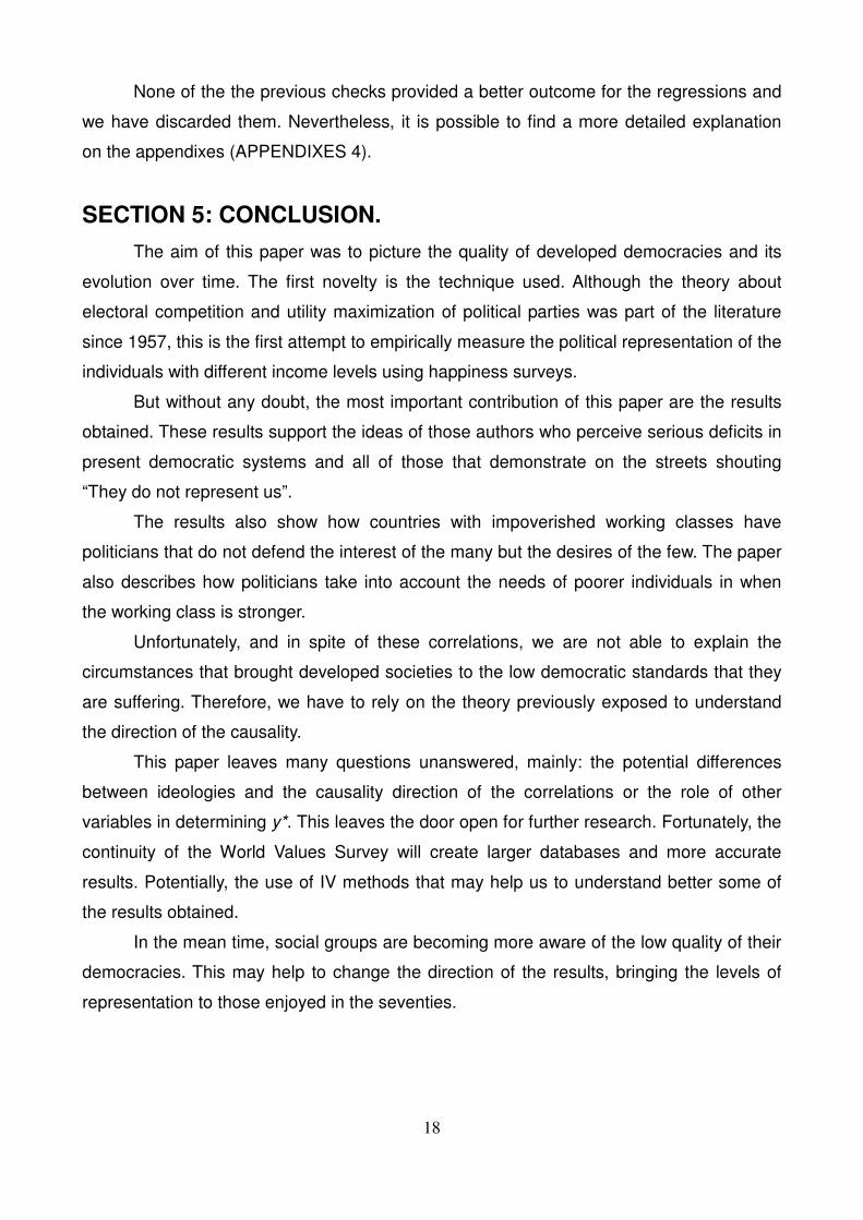
Graph 5 and Graph 6 show the income percentiles that different political parties

15

have maximized during the period of study (1981-2009) and they also include an

extrapolation (dashed in blue) till the moment that center governments represented the

median voter2.

<<Graph 5>>

<<Graph 6>>

As we can see, according to YEAR-3 and YEAR-4 the political situation in the

seventies is extremely similar to the description made by Crouch (2004).

4.2 Limitations

Even if the paper is able to show the huge democratic deficits of developed

countries, it fails in explaining the circumstances that have provoked this situation. It is true

that the coefficients of the regression COMP-4 are compatible with the theses of some

authors, but unfortunately, the coefficients just show correlation between y* and macro

variables, not the direction of the causality.

With the results obtained we could think that labor unions stop prevent the

politicians from favoring the economic elite, but it could be that countries with politicians

who favor the elite, create policies which weaken the labor unions. Similarly, it is possible

that countries with relative rich working classes are able to keep healthy democracies, but

it could also be that politicians who favor the richer take measures capable to worse the

economic situation of workers. This paper describes effectively the lack of democratic

levels but has its main limitation when trying to point out the causes of this situation.

We could understand better the direction of the causality by including newer waves

of the World Values Survey. Unfortunately, larger databases are more likely to generate

problems with the parallel-line assumption.

Finally, we would like to stress that both BASIC-3 and YEAR-3 present a very

peculiar selection of countries surveyed. Whereas WVS tries to have a fair representation

of the World, the data used from Schmitt (2011) considers only EU-12 countries for the

2 We consider that a democracy has a representative government when center parties represent the

median voter. A formal discussion is included in the appendixes (APPENDIXES 8)

16

period 1981-1986. This fact may generate the econometric differences shown in the result

table. On top of that, WVS suffered an important manipulation of the dependent variable

when we merged it with Schmitt (2011), as explained previously.

4.3 Robustness checks:

To sustain the validity of the previous results, we have carried out a long list of

robustness checks. Here, we will explain in detail those three that we consider more

important: The power of the polynomial, the lack of control for education levels, and the

symmetry-assumption. The rest will be commented at the end of this subsection and

shown in the appendixes (APPENDIXES 4).

4.3.1 Power of polynomial:

The regression assumes that utility function of a given individual is linked with a

polynomial of power two, recall:

ui ( yi , xk) = a·yi + b·y2i - ( ideo + ideo2) ·( d·yi - xk)

2

and it is estimated with

PUideo = β 3·ideoct+β 4·ideo2ct+β5·ideoct·yi,c,t+β6·ideoct · y

2i,c,t +β7·ideo2

ct·yi,c,t

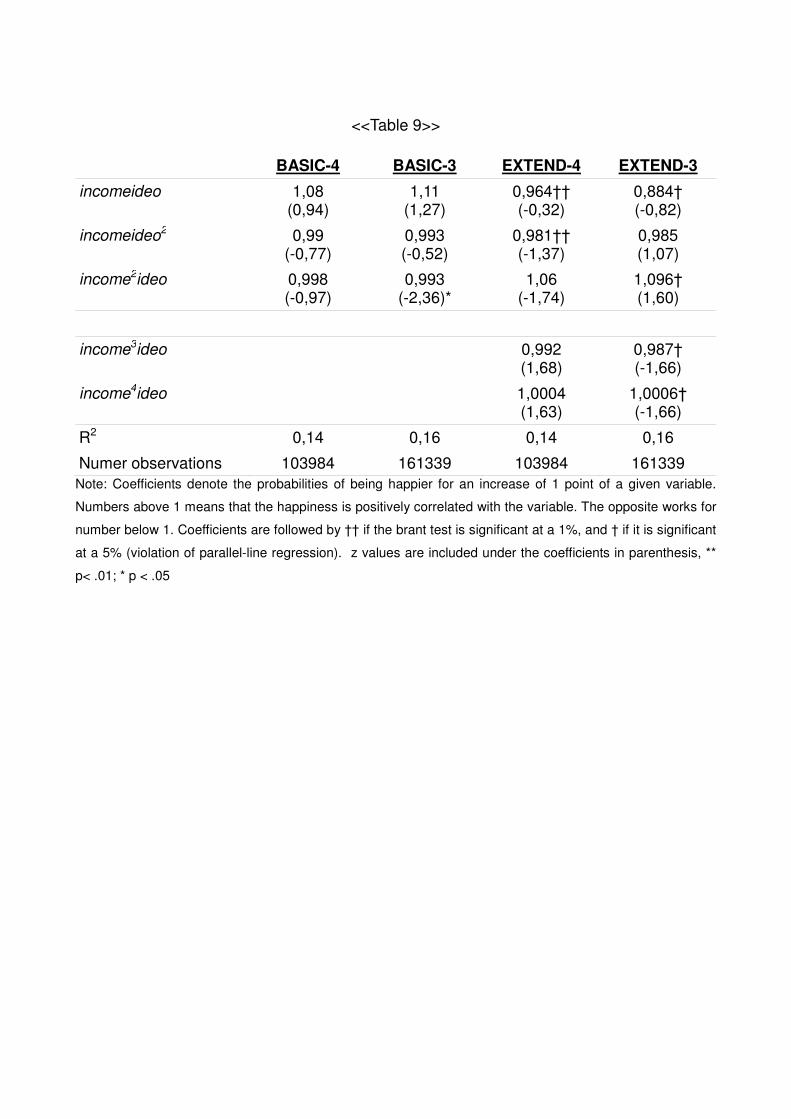
It is possible to argue that the polynomial has a higher power. This possibility has

been analyzed by considering not only income·ideo and income2·ideo, but also

income3·ideo and income4·ideo, in the BASIC3 and BASIC4 regressions.

As it can be seen in the appendixes (APPENDIX 5) these two variables are

insignificant. The introduction of these variables creates also serious problems to full-fill

the parallel-line assumption. On top of that, if we incorporate them in the analysis we

would need to interact both time (t) and the macro-variables (P) with them, making the

analysis unnecessary complicated. For all these reasons, we have decided not to include

them in the final regressions.

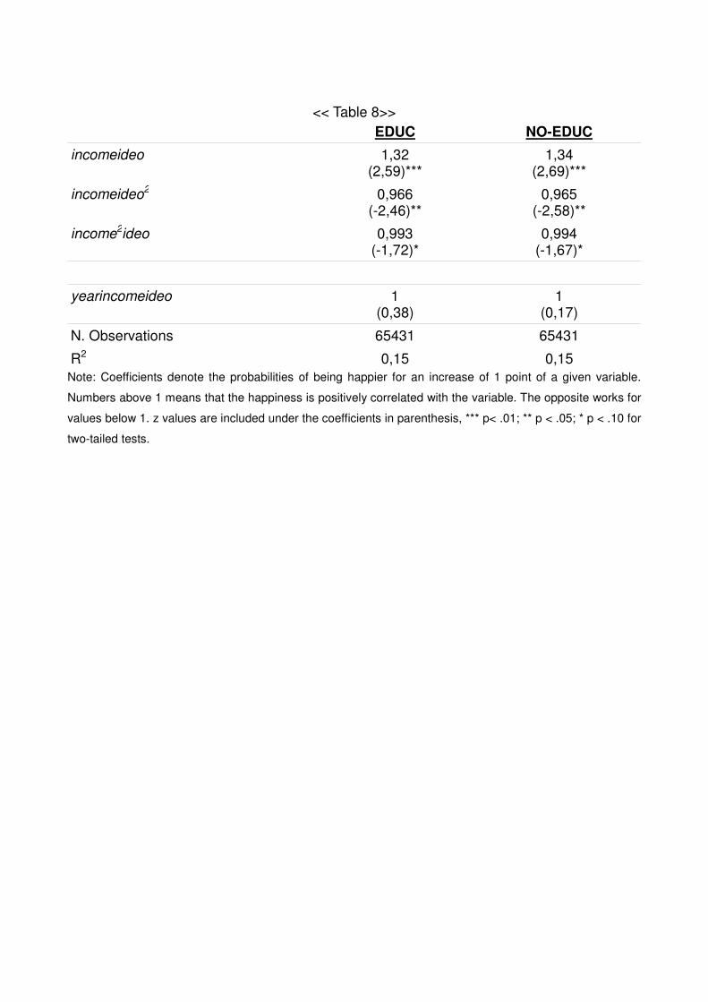
4.3.2 Education

The final regressions do not include a control for educational levels. Unfortunately,

the databases used do not provide educational information for all the individuals but only

for around 60.000. It is possible to imagine that education influences income, happiness,

and preferences for political parties. In order to measure the capacity of this variable to

17

change the results, we have carried out two regression only with the observations that

include education information. The first one, EDUC, includes an education variable and the

second one, NO-EDUC, does not.

As shown in appendixes (APPENDIXES 4) the introduction of measurements of

education does not change the results.

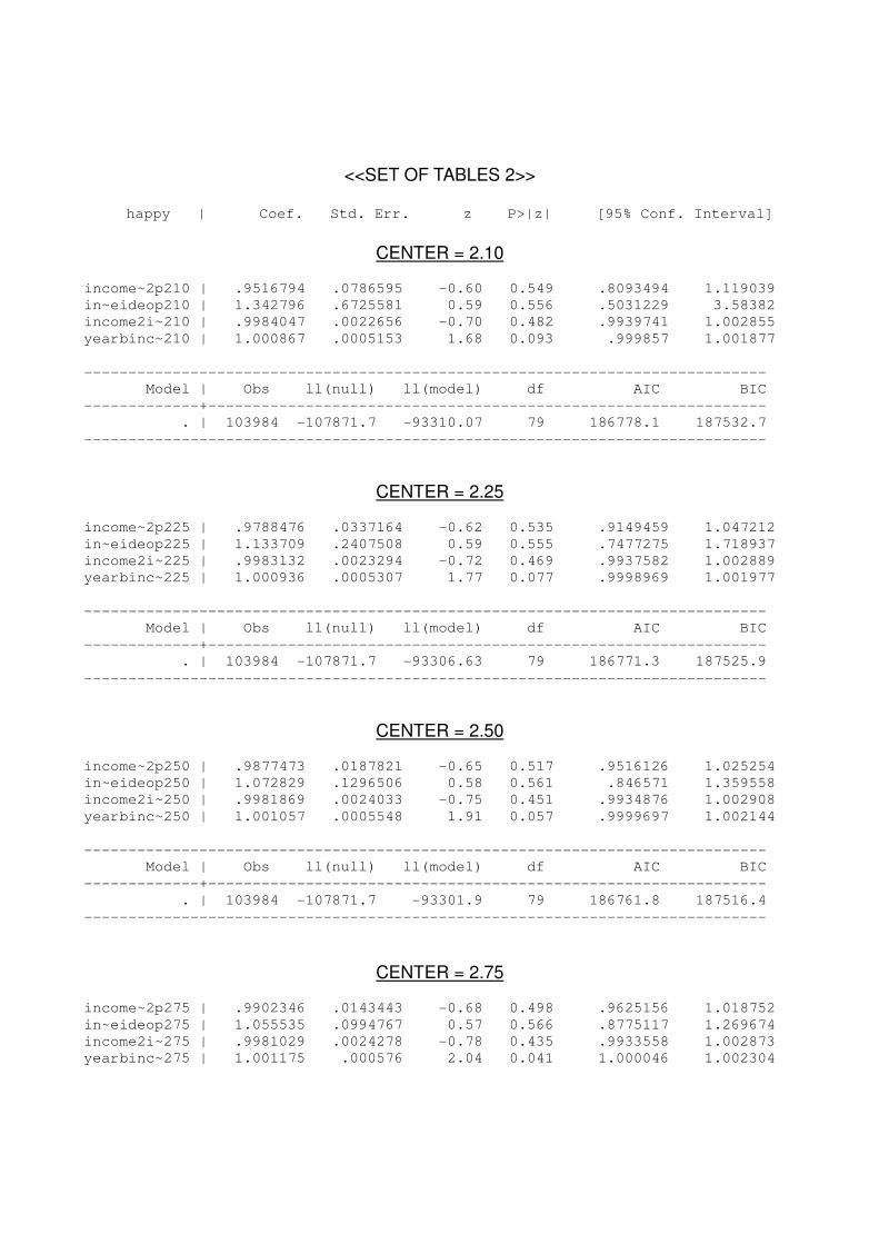
4.3.3 Symmetry

The values given to center-right, center and center-left governments are 2,3 and 4,

respectively. Therefore, the model assumes that the distance between center-left and

center ideologies is equal to the distance between center and center-right. We call this

consideration the symmetry-assumption. It is a strong assumption that may drive the

results.

It is possible to break the symmetry-assumption by adding of subtracting points to

the value given to the Center party. For instance, we can give the value 2.5 (-0.5) to Center

and see if the regression fits better.

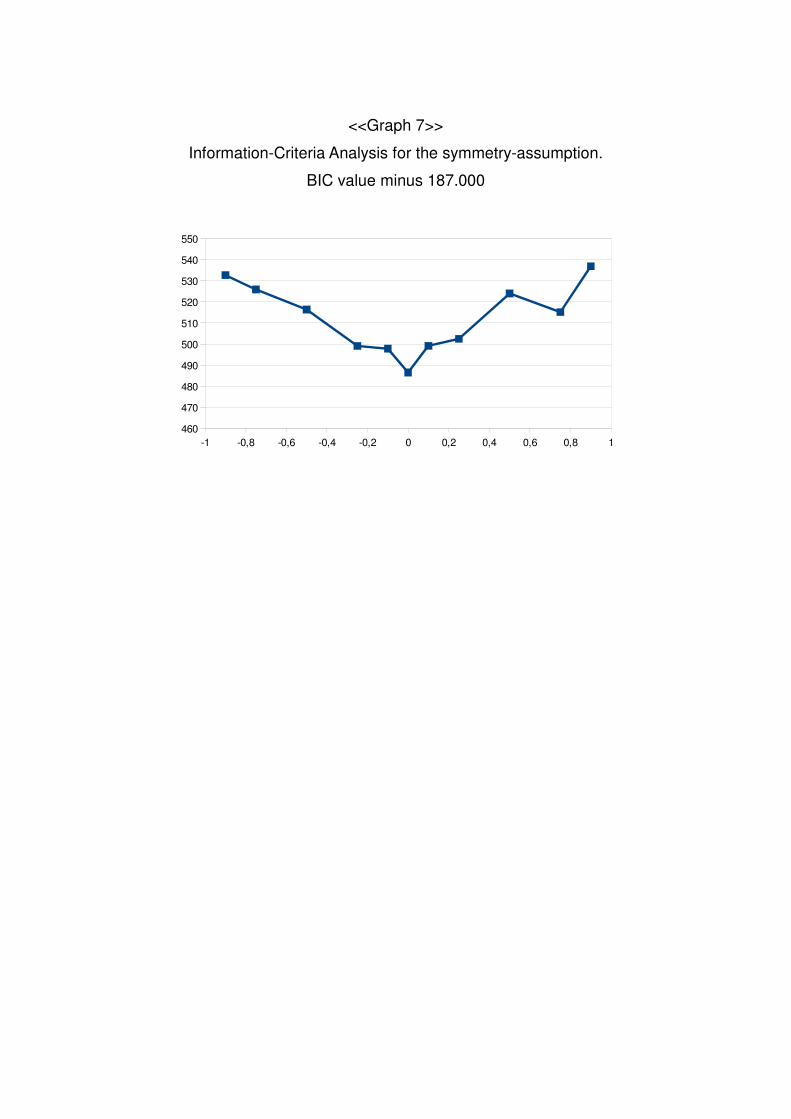
In order to analyze systematically the value of Center parties that fits better the

model we have replicated the YEAR4 regression modifying the value of Center parties with

a set of values. Those values are -0.9, -0.75, -0.5, -0.25, -0.1, +0, +0.1, +0.25, +0.5,

+0.75, +0.9. We carried out an information criteria analysis and the model with the lowest

value would be the best one. According to the information criteria analysis, the best fit

occurs with Center having value 3 (+0), meaning that symmetry is preferred.

Even when using the other values for Center parties, the final coefficients does not

change significantly. A summary of this check can be found in the appendixes (APPENDIX

6).

4.3.4 Other robustness checks:

We have also analyzed the possibility of a significant variable for income2·ideo2; the

interactions between age, gender and income; between ideo and employment dummies;

between income and employment dummies; the use of dummies for ideo values; we have

also measured the ideology of the parliament not only by the ideology of the present party

but also considering the ideology of the previous parties in government; we have split the

database by years, and we have tried several heteroskedasticity functions, finally we have

checked if the income distribution is homogeneous over time.

18

None of the the previous checks provided a better outcome for the regressions and

we have discarded them. Nevertheless, it is possible to find a more detailed explanation

on the appendixes (APPENDIXES 4).

SECTION 5: CONCLUSION.

The aim of this paper was to picture the quality of developed democracies and its

evolution over time. The first novelty is the technique used. Although the theory about

electoral competition and utility maximization of political parties was part of the literature

since 1957, this is the first attempt to empirically measure the political representation of the

individuals with different income levels using happiness surveys.

But without any doubt, the most important contribution of this paper are the results

obtained. These results support the ideas of those authors who perceive serious deficits in

present democratic systems and all of those that demonstrate on the streets shouting

“They do not represent us”.

The results also show how countries with impoverished working classes have

politicians that do not defend the interest of the many but the desires of the few. The paper

also describes how politicians take into account the needs of poorer individuals in when

the working class is stronger.

Unfortunately, and in spite of these correlations, we are not able to explain the

circumstances that brought developed societies to the low democratic standards that they

are suffering. Therefore, we have to rely on the theory previously exposed to understand

the direction of the causality.

This paper leaves many questions unanswered, mainly: the potential differences

between ideologies and the causality direction of the correlations or the role of other

variables in determining y*. This leaves the door open for further research. Fortunately, the

continuity of the World Values Survey will create larger databases and more accurate

results. Potentially, the use of IV methods that may help us to understand better some of

the results obtained.

In the mean time, social groups are becoming more aware of the low quality of their

democracies. This may help to change the direction of the results, bringing the levels of

representation to those enjoyed in the seventies.

19

REFERENCES:

Acemoglu, D. & Robinson, J. A, 2006. "Persistence of Power, Elites and Institutions,"

CEPR Discussion Papers 5603, C.E.P.R. Discussion Papers.

Agresti, A. 2000. Categorical data analysis. In: Wiley Series in Probability and Statistics,

2nd ed.

Alt, J. E & Lassen, D. D., 2010. Enforcement and Public Corruption: Evidence from US

States, EPRU Working Paper Series 2010-08, Economic Policy Research Unit (EPRU),

University of Copenhagen. Department of Economics.

Baldwin, R. E. and Robert-Nicoud, F. 2007. "Entry and Asymmetric Lobbying: Why

Governments Pick Losers, Journal of the European Economic Association, MIT Press, vol.

5(5), pages 1064-1093, 09.

Brant, R., 1990, Assessing Proportionality in the Proportional Odds Model for Ordinal

Logistic Regression, Biometrics, 35, 1171—1178.

Bühlmann, M., Merkel, W., Müller, L., Giebler, H. & Wessels, B., 2011. Democracy

Barometer. Methodology. Aarau: Zentrum für Demokratie.

Campbell,A., Converse, P. E.,&Rodgers,W. L. (1976).The quality of American life. New

York: Russell Sage.

Crouch, C., 2004. Post-Democracy. Cambridge: Polity Press.

Dreher, A. & Schneider, F., 2010. Corruption and the shadow economy: an empirical

analysis. Public Choice, Springer, vol. 144(1), pages 215-238, July.

Downs, A. 1957: An Economic Theory of Democracy, Harper and Row, New York (1957).

20

Edmond, C. 2011. Information Manipulation, Coordination, and Regime Change, NBER

Working Papers 17395, National Bureau of Economic Research, Inc.

Felli, L & Merlo, A. 2003. Endogenous Lobbying, STICERD - Theoretical Economics Paper

Series 448, Suntory and Toyota International Centres for Economics and Related

Disciplines, LSE.

Ferraz, C. & Finan, F., 2011. Electoral Accountability and Corruption: Evidence from the

Audits of Local Governments, American Economic Review, American Economic

Association, vol. 101(4), pages 1274-1311, June.

Freedom House. 2012. Freedom in the World: The Arab Uprisings and Their Global

Repercussions Selected data from Freedom House’s annual survey of political rights and

civil liberties. New York: Freedom House.

Frey, B & Stutzer, S. 2002. What Can Economists Learn from Happiness Research?

Journal of Economic Literature , Vol. 40, No. 2 (Jun., 2002), pp. 402-435. American

Economic Association

George, S., 2011. Whose Crisis, Whose Future? Towards a Greener, Fairer, Richer World.

Cambridge: Polity Press

Gundelach, P., & Kreiner, S. (2004). Happiness and life satisfaction in advanced European

countries. Cross-Cultural Research, 38(4), 359–386.

Kaufmann, D., Kraay, A. & Mastruzzi, M., 2009 Governance Matters VIII: Aggregate and

Individual Governance Indicators, 1996-2008 (June 29, 2009). World Bank Policy

Research Working Paper No. 4978. Available at SSRN: http://ssrn.com/abstract=1424591

Klein, N., 2007. The Shock Doctrine: The Rise of Disaster Capitalism. Toronto:Knopf

Canada.

Lane, R. E. (2000). The loss of happiness in market democracies. New Haven, CT: Yale

University Press.

21

Long, J. S. & Freese, J. 2001. Regression Models for Categorical Dependent Variables

Using Stata. Stata Press, 2001.

Potrafke, N., 2009. Did globalization restrict partisan politics? An empirical evaluation of

social expenditures in a panel of OECD countries, Public Choice, Springer, vol. 140(1),

pages 105-124, July.

Prat, A. & Strömberg, D., 2011. The Political Economy of Mass Media, CEPR Discussion

Papers 8246, C.E.P.R. Discussion Papers.

Revelle, C., Marks, D. & Liebman, J. C., 1970 An Analysis of Private and Public Sector

Location Models. Management Science , Vol. 16, No. 11, Theory Series (Jul., 1970), pp.

692-707

Evi, S. & Schmitt, H., 2001. The Mannheim Eurobarometer Trend File, 1970–99. Archived

at ICPSR: http://dx.doi.org/10.3886/ICPSR03384

Sirorta D, 2007. Hostile Takeover: How Big Money And Corruption Conquered Our

Government--And How We Take It. Ed: Three Rivers Press. ISBN-10: 0307237354

Stiglitz, Joseph E. 2011 "Of the 1%, by the 1%, for the 1%." Vanity Fair (2011): 1947-67.

Taibbi, M., 2010. Griftopia: Bubble Machines, Vampire Squids, and the Long Con That Is

Breaking America. Spiegel and Grau, New York.

Torija Jiménez, P. E., 2011. Stories on corruption. How media and prosecutors influence

elections, Marco Fanno Working Papers 0140, Dipartimento di Scienze Economiche

Marco Fanno.

Patty, J. W., Snyder, Y. & Ting, M. M., 2008. Two’s a Company, Three’s An Equilibrium:

Strategic Voting and Multicandidate Elections. Mimeo, Harvard University.

Urbinati, N, & Mark W., 2008. The concept of representation in democratic theory. The

22

Annual Review of Political Science 11: 387-412.

World Values Survey 1981-2008 OFFICIAL AGGREGATE v.20090901, 2009. World

Values Survey Association (www.worldvaluessurvey.org). Aggregate File Producer:

ASEP/JDS, Madrid.

Žižek, S. 2009. First as Tragedy, Then as Farce, London: Verso.

23

APPENDIXES

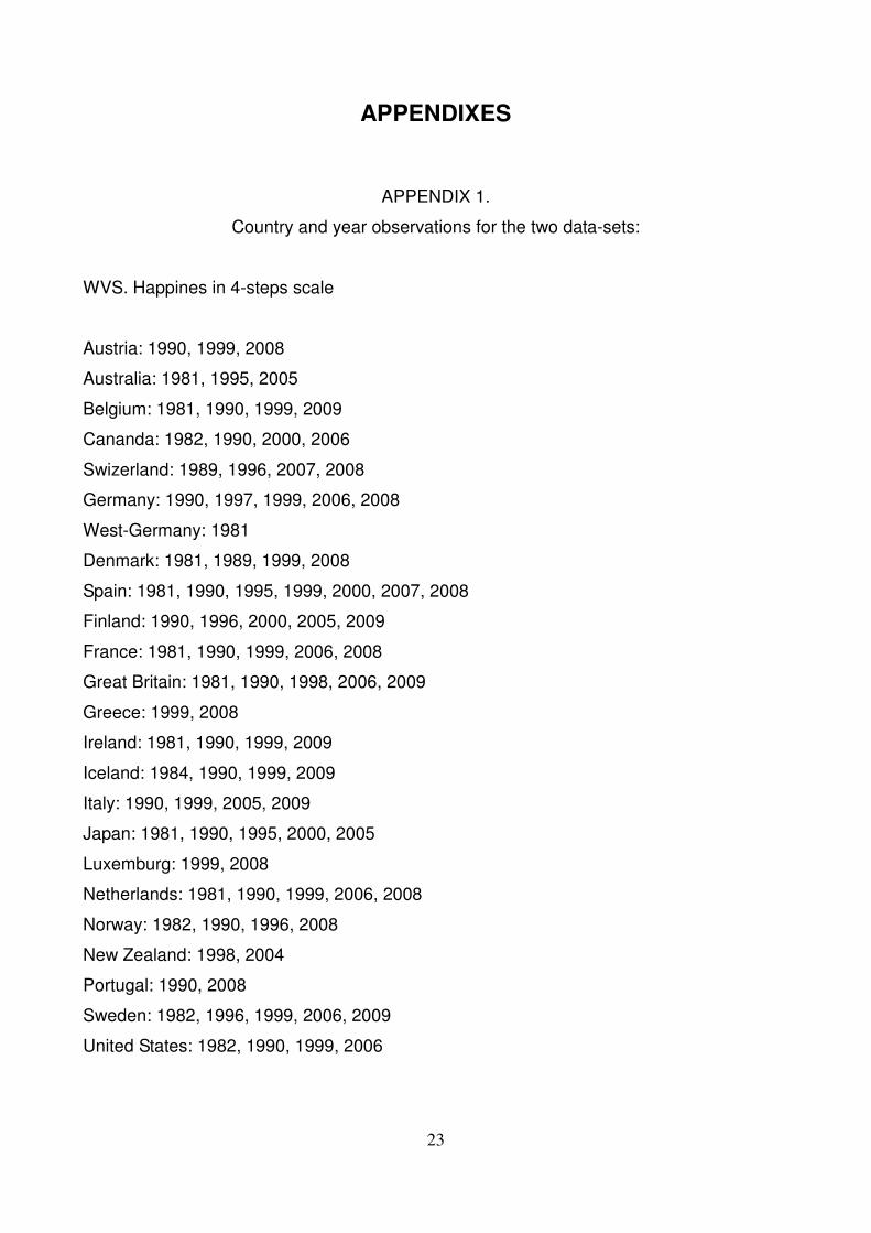
APPENDIX 1.

Country and year observations for the two data-sets:

WVS. Happines in 4-steps scale

Austria: 1990, 1999, 2008

Australia: 1981, 1995, 2005

Belgium: 1981, 1990, 1999, 2009

Cananda: 1982, 1990, 2000, 2006

Swizerland: 1989, 1996, 2007, 2008

Germany: 1990, 1997, 1999, 2006, 2008

West-Germany: 1981

Denmark: 1981, 1989, 1999, 2008

Spain: 1981, 1990, 1995, 1999, 2000, 2007, 2008

Finland: 1990, 1996, 2000, 2005, 2009

France: 1981, 1990, 1999, 2006, 2008

Great Britain: 1981, 1990, 1998, 2006, 2009

Greece: 1999, 2008

Ireland: 1981, 1990, 1999, 2009

Iceland: 1984, 1990, 1999, 2009

Italy: 1990, 1999, 2005, 2009

Japan: 1981, 1990, 1995, 2000, 2005

Luxemburg: 1999, 2008

Netherlands: 1981, 1990, 1999, 2006, 2008

Norway: 1982, 1990, 1996, 2008

New Zealand: 1998, 2004

Portugal: 1990, 2008

Sweden: 1982, 1996, 1999, 2006, 2009

United States: 1982, 1990, 1999, 2006

24

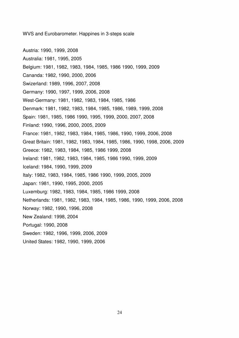
WVS and Eurobarometer. Happines in 3-steps scale

Austria: 1990, 1999, 2008

Australia: 1981, 1995, 2005

Belgium: 1981, 1982, 1983, 1984, 1985, 1986 1990, 1999, 2009

Cananda: 1982, 1990, 2000, 2006

Swizerland: 1989, 1996, 2007, 2008

Germany: 1990, 1997, 1999, 2006, 2008

West-Germany: 1981, 1982, 1983, 1984, 1985, 1986

Denmark: 1981, 1982, 1983, 1984, 1985, 1986, 1989, 1999, 2008

Spain: 1981, 1985, 1986 1990, 1995, 1999, 2000, 2007, 2008

Finland: 1990, 1996, 2000, 2005, 2009

France: 1981, 1982, 1983, 1984, 1985, 1986, 1990, 1999, 2006, 2008

Great Britain: 1981, 1982, 1983, 1984, 1985, 1986, 1990, 1998, 2006, 2009

Greece: 1982, 1983, 1984, 1985, 1986 1999, 2008

Ireland: 1981, 1982, 1983, 1984, 1985, 1986 1990, 1999, 2009

Iceland: 1984, 1990, 1999, 2009

Italy: 1982, 1983, 1984, 1985, 1986 1990, 1999, 2005, 2009

Japan: 1981, 1990, 1995, 2000, 2005

Luxemburg: 1982, 1983, 1984, 1985, 1986 1999, 2008

Netherlands: 1981, 1982, 1983, 1984, 1985, 1986, 1990, 1999, 2006, 2008

Norway: 1982, 1990, 1996, 2008

New Zealand: 1998, 2004

Portugal: 1990, 2008

Sweden: 1982, 1996, 1999, 2006, 2009

United States: 1982, 1990, 1999, 2006

25

APPENDIX 2.

Variables description

<< SET OF TABLES 1>>

26

APPENDIX 4.

Extra robustness cheks.

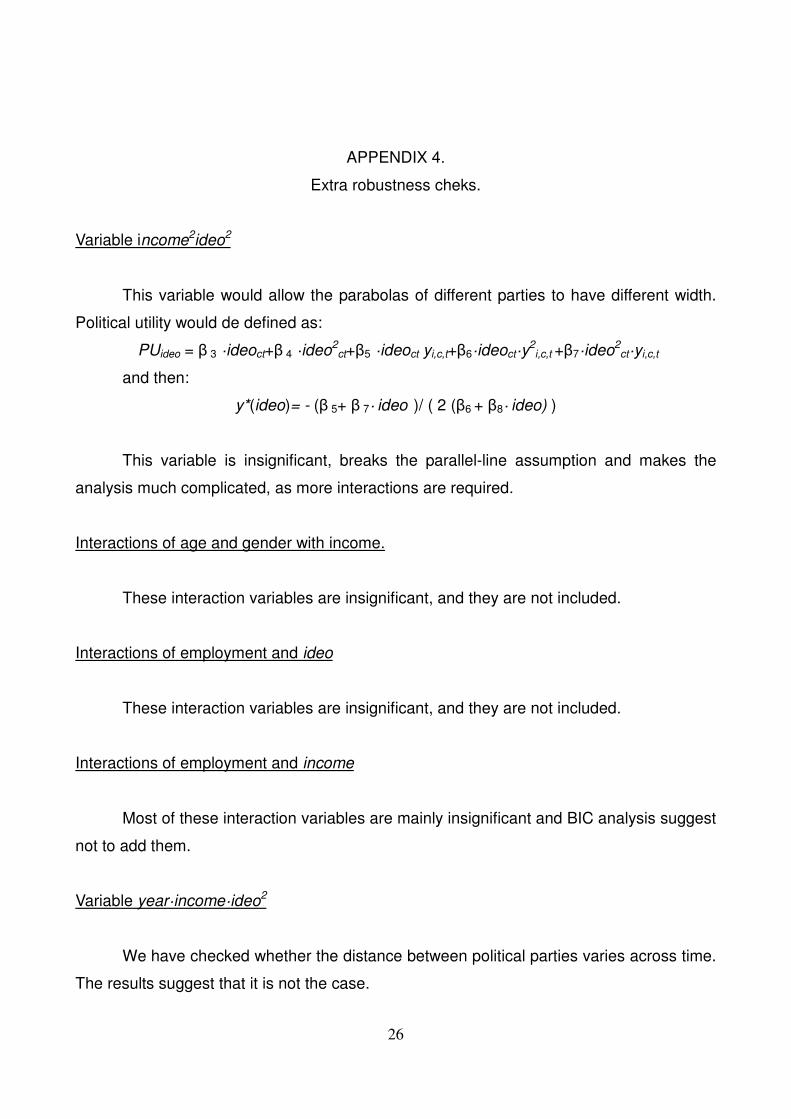
Variable income2ideo2

This variable would allow the parabolas of different parties to have different width.

Political utility would de defined as:

PUideo = β 3 ·ideoct+β 4 ·ideo2ct+β5 ·ideoct yi,c,t+β6·ideoct·y

2i,c,t +β7·ideo2

ct·yi,c,t

and then:

y*(ideo)= - (β 5+ β 7· ideo )/ ( 2 (β6 + β8· ideo) )

This variable is insignificant, breaks the parallel-line assumption and makes the

analysis much complicated, as more interactions are required.

Interactions of age and gender with income.

These interaction variables are insignificant, and they are not included.

Interactions of employment and ideo

These interaction variables are insignificant, and they are not included.

Interactions of employment and income

Most of these interaction variables are mainly insignificant and BIC analysis suggest

not to add them.

Variable year·income·ideo2

We have checked whether the distance between political parties varies across time.

The results suggest that it is not the case.

27

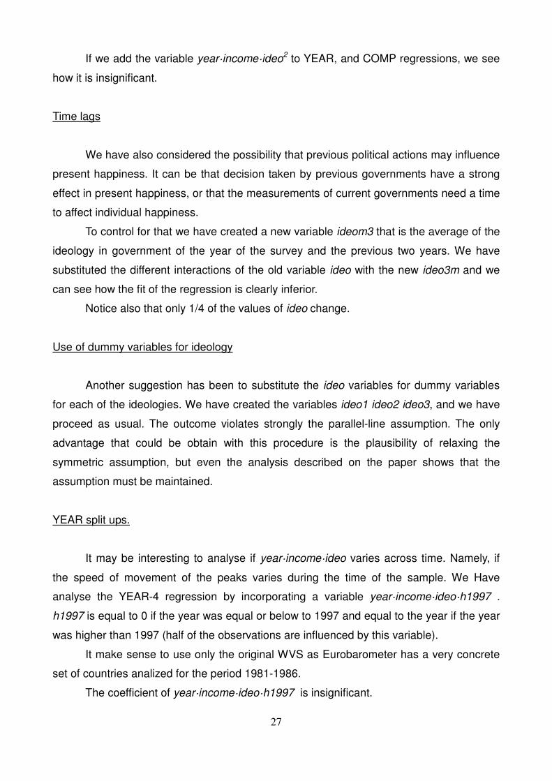
If we add the variable year·income·ideo2 to YEAR, and COMP regressions, we see

how it is insignificant.

Time lags

We have also considered the possibility that previous political actions may influence

present happiness. It can be that decision taken by previous governments have a strong

effect in present happiness, or that the measurements of current governments need a time

to affect individual happiness.

To control for that we have created a new variable ideom3 that is the average of the

ideology in government of the year of the survey and the previous two years. We have

substituted the different interactions of the old variable ideo with the new ideo3m and we

can see how the fit of the regression is clearly inferior.

Notice also that only 1/4 of the values of ideo change.

Use of dummy variables for ideology

Another suggestion has been to substitute the ideo variables for dummy variables

for each of the ideologies. We have created the variables ideo1 ideo2 ideo3, and we have

proceed as usual. The outcome violates strongly the parallel-line assumption. The only

advantage that could be obtain with this procedure is the plausibility of relaxing the

symmetric assumption, but even the analysis described on the paper shows that the

assumption must be maintained.

YEAR split ups.

It may be interesting to analyse if year·income·ideo varies across time. Namely, if

the speed of movement of the peaks varies during the time of the sample. We Have

analyse the YEAR-4 regression by incorporating a variable year·income·ideo·h1997 .

h1997 is equal to 0 if the year was equal or below to 1997 and equal to the year if the year

was higher than 1997 (half of the observations are influenced by this variable).

It make sense to use only the original WVS as Eurobarometer has a very concrete

set of countries analized for the period 1981-1986.

The coefficient of year·income·ideo·h1997 is insignificant.

28

Heteroskedasticity function

We have tried other forms of heteroskedasticity. We tried to include gdp, gini, and

income·ideo do to their capacities of highly influence the results. Other functions have

been rejected due to their requirements of computational power. All the coefficients of

these variables are insignificant when in the heteroskedasticity function.

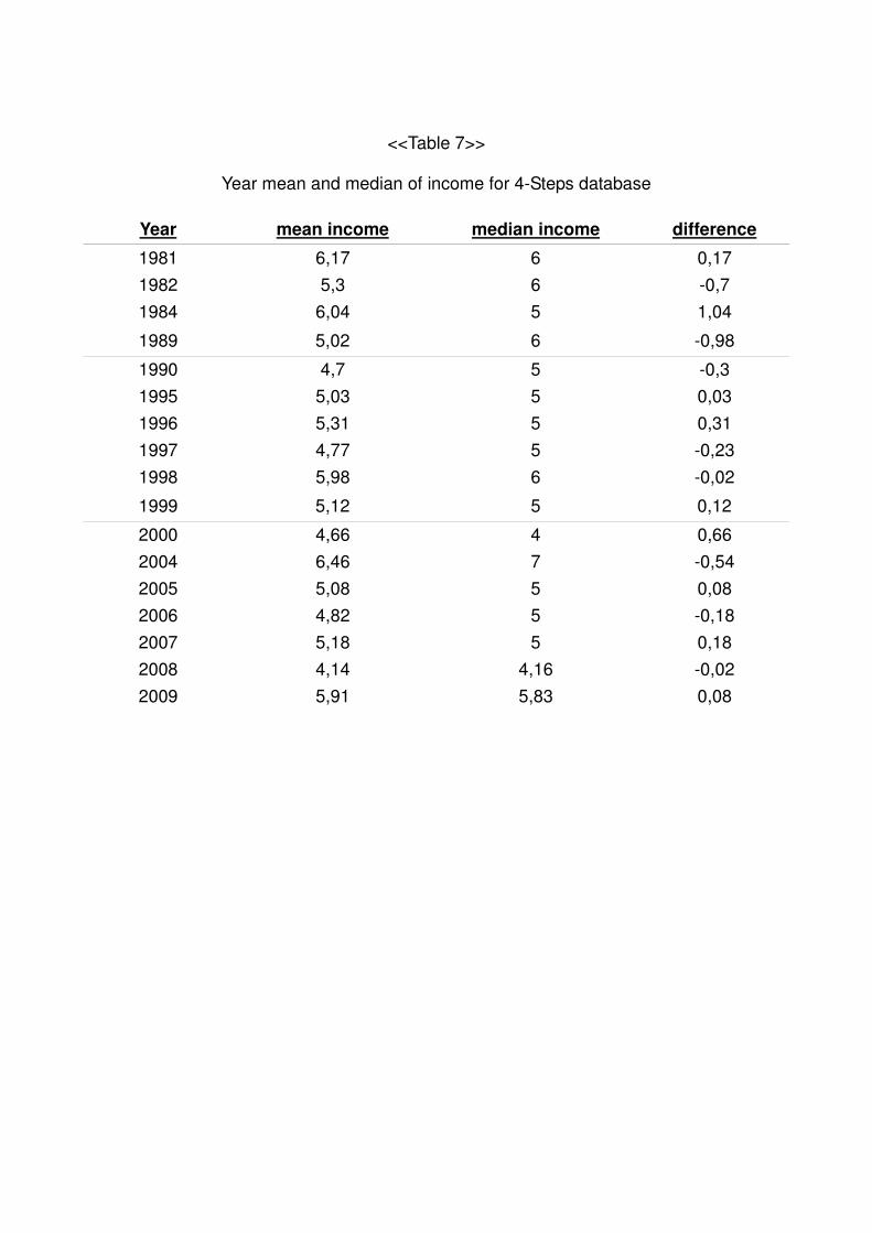
Distribution of income

Here is the mean and the median for income in a year basis. As we see there are

not time-tendencies.

<<Table 7>>

Education

Similarities of results when taking into account educational levels

<<Table 8>>

29

APPENDIX 5.

Detail: size of polynomial

Comparison between BASIC regression and the same regression with the inclusion

of income3ideo and income4ideo, labeled as EXTEND.

<<Table 9>>

30

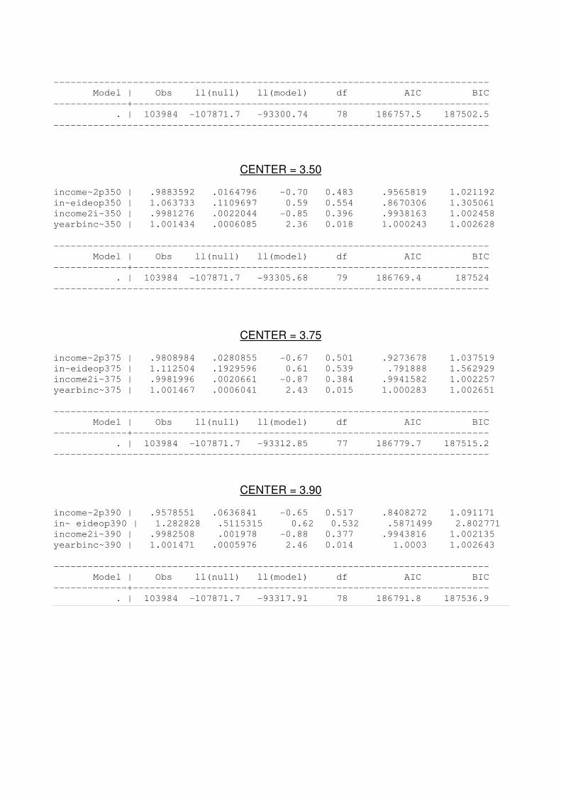
APPENDIX 6.

Detail: Symmetry-assumption

The values that determine the y* on the YEAR regression are: income·ideo,

income·ideo2, income2·ideo and year·income·ideo. Here we show the coefficients for

these variables for different values of Center. The IC analysis for each regression is also

shown.

<<SET OF TABLES 2>>

The following graph summarizes the BIC analysis for different values of Center

parties.

<<Graph 7>>

31

APPENDIX 7.

Distribution function of income

We have modified slightly the distribution functions of income, to go beyond the 11th

step of the income scale. For doing so, we have standardized the distribution function of

income to a negative binomial distribution that takes into account its mean and

overdispersion. These two parameters are fore each database:

<<Table 10>>

Following graph shows that distribution function for the two databases (happiness in

a 3-step and 4-step scale)

<<Graph8>>

32

APPENDIX 8.

Democratic representation

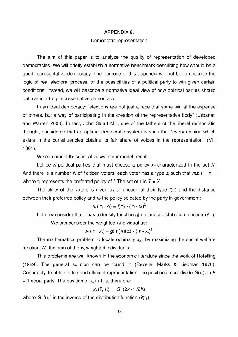
The aim of this paper is to analyze the quality of representation of developed

democracies. We will briefly establish a normative benchmark describing how should be a

good representative democracy. The purpose of this appendix will not be to describe the

logic of real electoral process, or the possibilities of a political party to win given certain

conditions. Instead, we will describe a normative ideal view of how political parties should

behave in a truly representative democracy.

In an ideal democracy: “elections are not just a race that some win at the expense

of others, but a way of participating in the creation of the representative body” (Urbanati

and Warren 2008). In fact, John Stuart Mill, one of the fathers of the liberal democratic

thought, considered that an optimal democratic system is such that “every opinion which

exists in the constituencies obtains its fair share of voices in the representation” (Mill

1861).

We can model these ideal views in our model, recall:

Let be K political parties that must choose a policy xk characterized in the set X.

And there is a number N of i citizen-voters, each voter has a type zi such that h(zi ) = τi ,

where τi represents the preferred policy of i. The set of τi is Τ = X.

The utility of the voters is given by a function of their type f(zi) and the distance

between their preferred policy and xk the policy selected by the party in government:

ui ( τi , xk) = f(zi) - ( τi - xk)2

Let now consider that τi has a density function g( τi ), and a distribution function G(τi).

We can consider the weighted i individual as:

wi ( τi , xk) = g( τi )/(f(zi) - ( τi - xk)2)

The mathematical problem to locale optimally xk , by maximizing the social welfare

function Wi, the sum of the wi weighted individuals:

This problems are well known in the economic literature since the work of Hotelling

(1929). The general solution can be found in (Revelle, Marks & Liebman 1970).

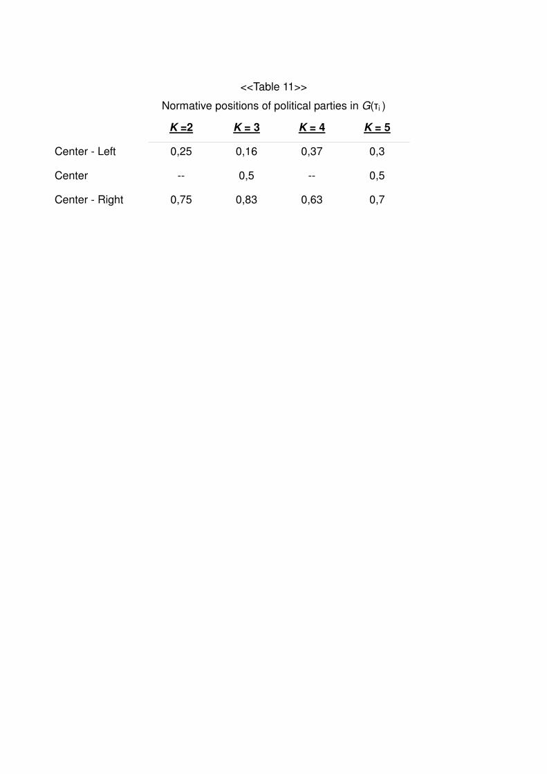
Concretely, to obtain a fair and efficient representation, the positions must divide G(τi ). in K

+ 1 equal parts. The position of xk in Τ is, therefore:

xk (Τ, K) = G-1(2k -1 /2K)

where G -1(τi ) is the inverse of the distribution function G(τi ).

33

We can tabulate the position of center-left, center and center-right3 parties for

different values of K.

<<Table 11>>

As we can see the best way of measuring whether there is a good level of

representation is to analyze whether center parties maximize the utility of the median voter

(0,5).

3 We consider center-left and center-right to the immediate inferior and superior k parties to the median of

K

34

TABLES AND FIGURES

GRAPH 1

Downs model visually

GRAPH 2

Explaining the econometric model

<<GRAPH 3>>

Relationship between the latent variable Y* and Y.

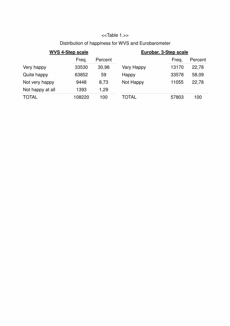
<<Table 1.>>

Distribution of happiness for WVS and Eurobarometer

WVS 4-Step scale Eurobar. 3-Step scale

Freq. Percent Freq. Percent

Very happy 33530 30,98 Vary Happy 13170 22,78

Quite happy 63852 59 Happy 33578 58,09

Not very happy 9448 8,73 Not Happy 11055 22,78

Not happy at all 1393 1,29

TOTAL 108220 100 TOTAL 57803 100

<<Table 2>> Results table

Ordinal generalized logistic model. Dependent variable: Level of Happiness.

BASIC-4 BASIC-3 YEAR-4 YEAR-3 NOCO-4 COMP-4

income·ideo 0,08 (0,94)

0,11 (1,27)

0,05 (0,57)

0,09 (1,03)

0,52 † (3,02)***

1,02 (3,59)***

income·ideo2 -0,01 (-0,77)

-0,007 (-0,52)

-0,009 (-0,70)

-0,009 (-0,76)

-0,028 †† (-2,45)**

-0,046 †† (-2,88)***

income2·ideo -0,002 (-0,97)

-0,007 (-2,36)**

-0,002 (-0,80)

-0,006 (-2,00)**

-0,002 (-0,89)

-0,002 (-0,76)

year·income·ideo 0,0013 (2,16)**

0,0017 (2,96)***

0 (-0,03)

0,0003 (0,27)

wagessh·income·ideo -0,413 (-2,41)**

-0,402 (-3,26)***

labor·income·ideo -0,03 (-1,16)

-0,054 (-1,67)*

Controls interacting with income·ideo

NO NO NO NO NO YES

R2 0,14 0,16 0,14 0,16 0,14 0,14

N. Observations 103984 161339 103984 161339 103984 103984 Note: Coefficients denote the probabilities of being happier for an increase of 1 point of a given

variable. Coefficients are followed by †† if the brant test is significant at a 1%, and † if it is significant at a

5% (violation of parallel-line regression). z values are included under the coefficients in parenthesis, *** p<

.01; ** p < .05; * p < .10 for two-tailed tests.

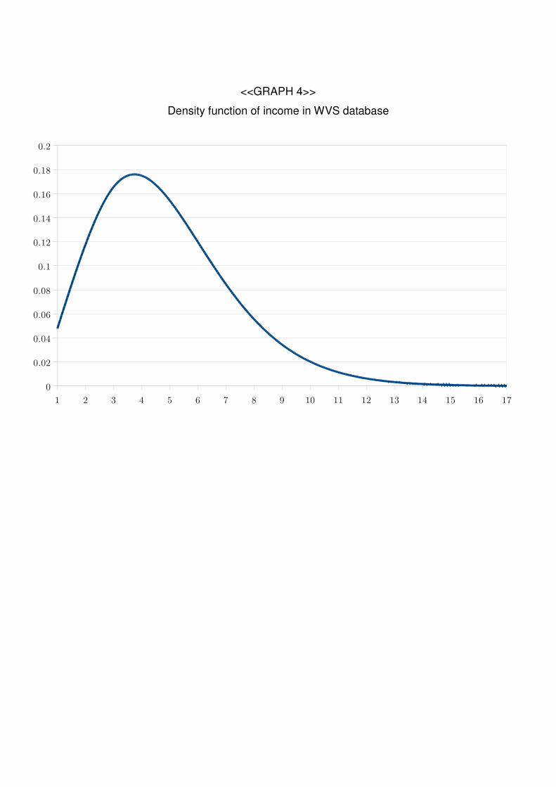
<<GRAPH 4>>

Density function of income in WVS database

1 2 3 4 5 6 7 8 9 10 11 12 13 14 15 16 17

0

0.02

0.04

0.06

0.08

0.1

0.12

0.14

0.16

0.18

0.2

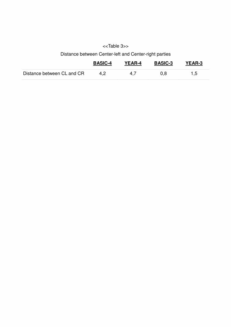
<<Table 3>>

Distance between Center-left and Center-right parties

BASIC-4 YEAR-4 BASIC-3 YEAR-3

Distance between CL and CR 4,2 4,7 0,8 1,5

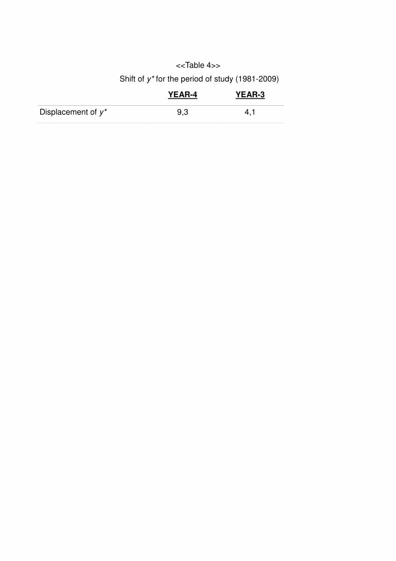
<<Table 4>>

Shift of y* for the period of study (1981-2009)

YEAR-4 YEAR-3

Displacement of y* 9,3 4,1

<<Table 5>>

Correlations between y* and statistically significant variables

Increase of 1% Increase 1 st. dev.

Wages share (wagessh) -1,17 -6,28

Affiliation to Labor Unions (labor) -0,15 -3,4

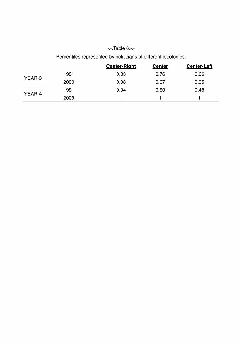
<<Table 6>>

Percentiles represented by politicians of different ideologies.

Center-Right Center Center-Left

YEAR-3 1981 0,83 0,76 0,66

2009 0,98 0,97 0,95

YEAR-4 1981 0,94 0,80 0,48

2009 1 1 1

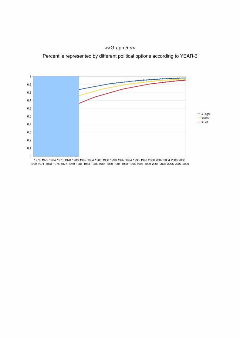
<<Graph 5.>>

Percentile represented by different political options according to YEAR-3

19691970

19711972

19731974

19751976

19771978

19791980

19811982

19831984

19851986

19871988

19891990

19911992

19931994

19951996

19971998

19992000

20012002

20032004

20052006

20072008

2009

0

0,1

0,2

0,3

0,4

0,5

0,6

0,7

0,8

0,9

1

C-RightCenterC-Left

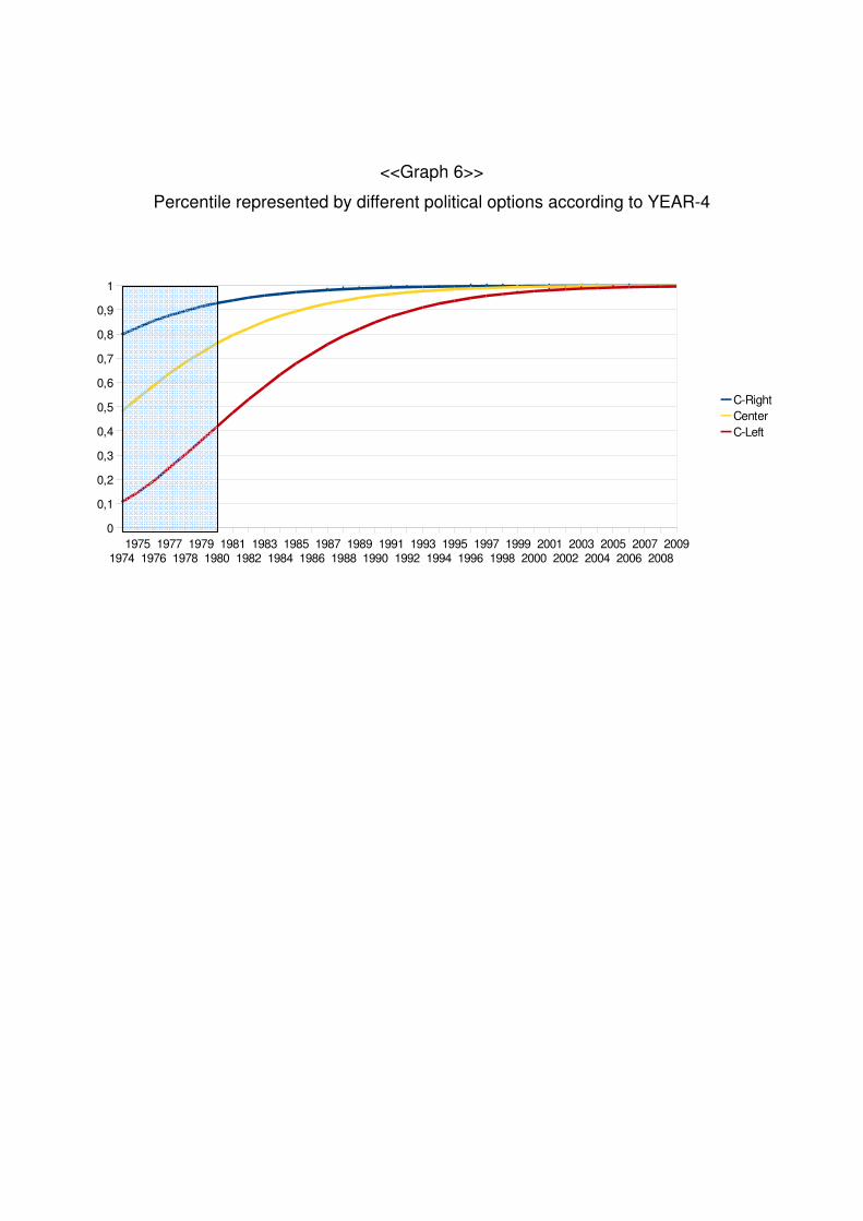
<<Graph 6>>

Percentile represented by different political options according to YEAR-4

19741975

19761977

19781979

19801981

19821983

19841985

19861987

19881989

19901991

19921993

19941995

19961997

19981999

20002001

20022003

20042005

20062007

20082009

0

0,1

0,2

0,3

0,4

0,5

0,6

0,7

0,8

0,9

1

C-RightCenterC-Left

<< SET OF TABLES 1>>

Variable description

Main variables from WVS 4-Step data-set Variable | Obs Mean Std. Dev. Min Max

-------------+--------------------------------------------------------

income | 108223 5.32804 2.518458 .8333333 11

parl | 107184 2.878293 .8290044 2 4

gdp | 108223 2.857797 .8294909 1.3 7.38

wagessh | 108223 .5951313 .053495 .459 .723

turnout | 108223 .7804567 .1067069 .4225 .9575

-------------+--------------------------------------------------------

growth | 108223 .0205479 .0295204 -.084 .099

labor | 108223 .3639272 .2166133 .076 .93

unemp | 108223 .0750684 .0372259 .02 .227

gini | 108223 .2949596 .0412372 .2 .39

unieduc | 108223 .4986948 .194867 .105 .919

| income parl gdp wagessh turnout

-------------+---------------------------------------------

income | 1.0000

parl | -0.0039 1.0000

gdp | 0.0627 0.0369 1.0000

wagessh | 0.0251 -0.0767 -0.4516 1.0000

turnout | 0.0006 -0.0428 0.0006 -0.2073 1.0000

growth | -0.0955 0.1005 -0.0505 -0.0862 -0.1348

labor | 0.0696 -0.0270 0.0074 -0.1314 0.2492

unemp | -0.0956 0.1977 -0.4129 0.0695 0.0626

gini | -0.0345 0.0379 -0.1539 0.0640 -0.1791

unieduc | -0.0159 0.0335 0.2587 -0.2849 -0.0499

| growth labor unemp gini unieduc

-------------+---------------------------------------------

growth | 1.0000

labor | -0.0585 1.0000

unemp | -0.0354 -0.2017 1.0000

gini | -0.0137 -0.6469 0.3487 1.0000

unieduc | -0.1869 0.0451 0.0073 0.0749 1.0000

Main variables from WVS and Eurobarometer, 3-Step data-set Variable | Obs Mean Std. Dev. Min Max

-------------+--------------------------------------------------------

income | 166360 5.277903 2.53724 .8333333 11

parl | 166360 2.827212 .8397685 2 4

<<Table 7>>

Year mean and median of income for 4-Steps database

Year mean income median income difference

1981 6,17 6 0,17

1982 5,3 6 -0,7

1984 6,04 5 1,04

1989 5,02 6 -0,98

1990 4,7 5 -0,3

1995 5,03 5 0,03

1996 5,31 5 0,31

1997 4,77 5 -0,23

1998 5,98 6 -0,02

1999 5,12 5 0,12

2000 4,66 4 0,66

2004 6,46 7 -0,54

2005 5,08 5 0,08

2006 4,82 5 -0,18

2007 5,18 5 0,18

2008 4,14 4,16 -0,02

2009 5,91 5,83 0,08

<< Table 8>> EDUC NO-EDUC

incomeideo 1,32 (2,59)***

1,34 (2,69)***

incomeideo2 0,966 (-2,46)**

0,965 (-2,58)**

income2ideo 0,993 (-1,72)*

0,994 (-1,67)*

yearincomeideo 1 (0,38)

1 (0,17)

N. Observations 65431 65431

R2 0,15 0,15 Note: Coefficients denote the probabilities of being happier for an increase of 1 point of a given variable.

Numbers above 1 means that the happiness is positively correlated with the variable. The opposite works for

values below 1. z values are included under the coefficients in parenthesis, *** p< .01; ** p < .05; * p < .10 for

two-tailed tests.

<<Table 9>> BASIC-4 BASIC-3 EXTEND-4 EXTEND-3

incomeideo 1,08 (0,94)

1,11 (1,27)

0,964†† (-0,32)

0,884† (-0,82)

incomeideo2 0,99 (-0,77)

0,993 (-0,52)

0,981†† (-1,37)

0,985 (1,07)

income2ideo 0,998 (-0,97)

0,993 (-2,36)*

1,06 (-1,74)

1,096† (1,60)

income3ideo 0,992 (1,68)

0,987† (-1,66)

income4ideo 1,0004 (1,63)

1,0006† (-1,66)

R2 0,14 0,16 0,14 0,16

Numer observations 103984 161339 103984 161339 Note: Coefficients denote the probabilities of being happier for an increase of 1 point of a given variable.

Numbers above 1 means that the happiness is positively correlated with the variable. The opposite works for

number below 1. Coefficients are followed by †† if the brant test is significant at a 1%, and † if it is significant

at a 5% (violation of parallel-line regression). z values are included under the coefficients in parenthesis, **

p< .01; * p < .05

<<SET OF TABLES 2>> happy | Coef. Std. Err. z P>|z| [95% Conf. Interval]

CENTER = 2.10

income~2p210 | .9516794 .0786595 -0.60 0.549 .8093494 1.119039

in~eideop210 | 1.342796 .6725581 0.59 0.556 .5031229 3.58382

income2i~210 | .9984047 .0022656 -0.70 0.482 .9939741 1.002855

yearbinc~210 | 1.000867 .0005153 1.68 0.093 .999857 1.001877

-----------------------------------------------------------------------------

Model | Obs ll(null) ll(model) df AIC BIC

-------------+---------------------------------------------------------------

. | 103984 -107871.7 -93310.07 79 186778.1 187532.7

-----------------------------------------------------------------------------

CENTER = 2.25 income~2p225 | .9788476 .0337164 -0.62 0.535 .9149459 1.047212

in~eideop225 | 1.133709 .2407508 0.59 0.555 .7477275 1.718937

income2i~225 | .9983132 .0023294 -0.72 0.469 .9937582 1.002889

yearbinc~225 | 1.000936 .0005307 1.77 0.077 .9998969 1.001977

-----------------------------------------------------------------------------

Model | Obs ll(null) ll(model) df AIC BIC

-------------+---------------------------------------------------------------

. | 103984 -107871.7 -93306.63 79 186771.3 187525.9

-----------------------------------------------------------------------------

CENTER = 2.50 income~2p250 | .9877473 .0187821 -0.65 0.517 .9516126 1.025254

in~eideop250 | 1.072829 .1296506 0.58 0.561 .846571 1.359558

income2i~250 | .9981869 .0024033 -0.75 0.451 .9934876 1.002908

yearbinc~250 | 1.001057 .0005548 1.91 0.057 .9999697 1.002144

-----------------------------------------------------------------------------

Model | Obs ll(null) ll(model) df AIC BIC

-------------+---------------------------------------------------------------

. | 103984 -107871.7 -93301.9 79 186761.8 187516.4

-----------------------------------------------------------------------------

CENTER = 2.75 income~2p275 | .9902346 .0143443 -0.68 0.498 .9625156 1.018752

in~eideop275 | 1.055535 .0994767 0.57 0.566 .8775117 1.269674

income2i~275 | .9981029 .0024278 -0.78 0.435 .9933558 1.002873

yearbinc~275 | 1.001175 .000576 2.04 0.041 1.000046 1.002304

-----------------------------------------------------------------------------

Model | Obs ll(null) ll(model) df AIC BIC

-------------+---------------------------------------------------------------

. | 103984 -107871.7 -93299 78 186754 187499.1

-----------------------------------------------------------------------------

CENTER = 2.90 income~2p290 | .9907808 .0132516 -0.69 0.489 .9651455 1.017097

in~eideop290 | 1.051218 .0920663 0.57 0.568 .8854093 1.248077

income2i~290 | .9980764 .0024166 -0.80 0.426 .9933512 1.002824

yearbinc~290 | 1.001241 .0005869 2.12 0.034 1.000092 1.002392

-----------------------------------------------------------------------------

Model | Obs ll(null) ll(model) df AIC BIC

-------------+---------------------------------------------------------------

. | 103984 -107871.7 -93298.38 78 186752.8 187497.8

-----------------------------------------------------------------------------

CENTER = 3,00 => SYMMETRY

income~2p300 | .9909014 .0129289 -0.70 0.484 .9658824 1.016568

in~eideop300 | 1.049885 .0897204 0.57 0.569 .8879737 1.241318

income2i~300 | .9980685 .0023986 -0.80 0.421 .9933785 1.002781

yearbinc~300 | 1.001283 .0005932 2.16 0.030 1.000121 1.002446

-----------------------------------------------------------------------------

Model | Obs ll(null) ll(model) df AIC BIC

-------------+---------------------------------------------------------------

. | 103984 -107871.7 -93298.5 77 186751 187486.5

-----------------------------------------------------------------------------

CENTER = 3.10 income~2p310 | .9908518 .0128906 -0.71 0.480 .965906 1.016442

in~eideop310 | 1.049639 .0891445 0.57 0.568 .8886864 1.239742

income2i~310 | .9980683 .0023725 -0.81 0.416 .9934292 1.002729

yearbinc~310 | 1.001321 .0005985 2.21 0.027 1.000149 1.002495

-----------------------------------------------------------------------------

Model | Obs ll(null) ll(model) df AIC BIC

-------------+---------------------------------------------------------------

. | 103984 -107871.7 -93299.06 78 186754.1 187499.2

-----------------------------------------------------------------------------

CENTER = 3.25

income~2p325 | .9904371 .0133984 -0.71 0.478 .9645218 1.017049

in~eideop325 | 1.051484 .0918205 0.57 0.565 .8860781 1.247768

income2i~325 | .9980806 .00232 -0.83 0.408 .9935437 1.002638

yearbinc~325 | 1.001372 .0006046 2.27 0.023 1.000188 1.002558

-----------------------------------------------------------------------------

Model | Obs ll(null) ll(model) df AIC BIC

-------------+---------------------------------------------------------------

. | 103984 -107871.7 -93300.74 78 186757.5 187502.5

-----------------------------------------------------------------------------

CENTER = 3.50 income~2p350 | .9883592 .0164796 -0.70 0.483 .9565819 1.021192

in~eideop350 | 1.063733 .1109697 0.59 0.554 .8670306 1.305061

income2i~350 | .9981276 .0022044 -0.85 0.396 .9938163 1.002458

yearbinc~350 | 1.001434 .0006085 2.36 0.018 1.000243 1.002628

-----------------------------------------------------------------------------

Model | Obs ll(null) ll(model) df AIC BIC

-------------+---------------------------------------------------------------

. | 103984 -107871.7 -93305.68 79 186769.4 187524

-----------------------------------------------------------------------------

CENTER = 3.75

income~2p375 | .9808984 .0280855 -0.67 0.501 .9273678 1.037519

in~eideop375 | 1.112504 .1929596 0.61 0.539 .791888 1.562929

income2i~375 | .9981996 .0020661 -0.87 0.384 .9941582 1.002257

yearbinc~375 | 1.001467 .0006041 2.43 0.015 1.000283 1.002651

-----------------------------------------------------------------------------

Model | Obs ll(null) ll(model) df AIC BIC

-------------+---------------------------------------------------------------

. | 103984 -107871.7 -93312.85 77 186779.7 187515.2

-----------------------------------------------------------------------------

CENTER = 3.90 income~2p390 | .9578551 .0636841 -0.65 0.517 .8408272 1.091171

in~ eideop390 | 1.282828 .5115315 0.62 0.532 .5871499 2.802771

income2i~390 | .9982508 .001978 -0.88 0.377 .9943816 1.002135

yearbinc~390 | 1.001471 .0005976 2.46 0.014 1.0003 1.002643

-----------------------------------------------------------------------------

Model | Obs ll(null) ll(model) df AIC BIC

-------------+---------------------------------------------------------------

. | 103984 -107871.7 -93317.91 78 186791.8 187536.9

<<Graph 7>>

Information-Criteria Analysis for the symmetry-assumption.

BIC value minus 187.000

-1 -0,8 -0,6 -0,4 -0,2 0 0,2 0,4 0,6 0,8 1460

470

480

490

500

510

520

530

540

550

<<Table 10>>

Income distribution for the two databases

Distribution function

Income 3 - Steps 4 - Steps

1 0,07617 0,04785

2 0,22326 0,16546

3 0,42248 0,33098

4 0,60000 0,50594

5 0,74123 0,66025

6 0,84165 0,78013

7 0,90746 0,86487

8 0,94796 0,92053

9 0,97167 0,95499

10 0,98501 0,97533

11 0,99225 0,98686

12 0,99608 0,99318

13 0,99805 0,99653

14 0,99905 0,99827

15 0,99954 0,99916

16 0,99978 0,99959

17 0,99990 0,99980

18 0,99990 0,99990

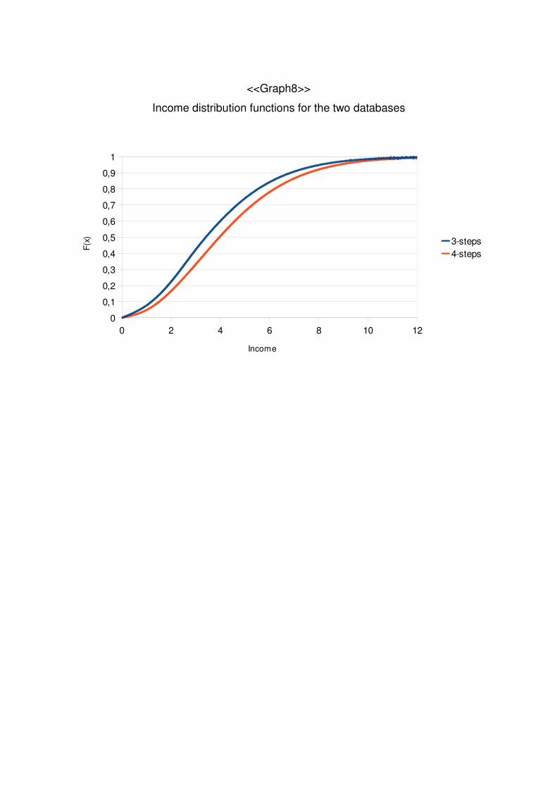
<<Graph8>>

Income distribution functions for the two databases

0 2 4 6 8 10 120

0,1

0,2

0,3

0,4

0,5

0,6

0,7

0,8

0,9

1

3-steps4-steps

Income

F(x)

<<Table 11>>

Normative positions of political parties in G(τi )

K =2 K = 3 K = 4 K = 5

Center - Left 0,25 0,16 0,37 0,3

Center -- 0,5 -- 0,5

Center - Right 0,75 0,83 0,63 0,7