civil depth notes for mar 15th-soil

FE DS Civil Review Soil Mechanics and Foundations

i

Table of Contents

1.0 Index Properties and Soil Classification .......................................................... 1

1.1 Index Properties ................................................................................................. 1 1.2 AASHTO Classification System ........................................................................ 4

EXAMPLE 1-2 .................................................................................................. 5 1.3 Unified Soil Classification System (USCS)....................................................... 6

EXAMPLE 1-3 .................................................................................................. 8

2.0 Phase Relationships .......................................................................................... 9 EXAMPLE 2-1 ................................................................................................ 12 EXAMPLE 2-2 ................................................................................................ 13

3.0 Laboratory and Field Tests .............................................................................. 15 3.1 Proctor Laboratory Tests ................................................................................. 16

4.0 Vertical Total and Effective Stress .................................................................. 18 4.1 Total Vertical Stress ......................................................................................... 18

4.2 Pore Water Pressure ........................................................................................ 19 4.3 Effective Vertical Stress ................................................................................... 20

EXAMPLE 4-1 ................................................................................................ 20 5.0 Retaining Walls ................................................................................................. 21

5.1 Earth Pressure Introduction ............................................................................ 21 5.2 Rankine Earth Pressure Theory ...................................................................... 21

EXAMPLE 5-1 ................................................................................................ 22 EXAMPLE 5-2 ................................................................................................ 23

6.0 Shear Strength .................................................................................................. 24 6.1 Intro to Shear Strength Parameters ................................................................ 24

7.0 Shallow Spread Foundations .......................................................................... 26 7.1 Types of Foundations ...................................................................................... 26 7.2 General Bearing Capacity Theory ................................................................... 26

EXAMPLE 7-1 ................................................................................................ 27 EXAMPLE 7-2 ............................................................................................... 27

8.0 Consolidation .................................................................................................... 28 8.1 Load Distribution in Soils ................................................................................ 28

EXAMPLE 8-1 ................................................................................................ 28

EXAMPLE 8-2 ................................................................................................ 28 EXAMPLE 8-3 ................................................................................................ 29

8.2 Consolidation in Clay Soils ............................................................................. 30 8.3 Rate of Consolidation ...................................................................................... 32

EXAMPLE 8-4 ................................................................................................ 33 9.0 Permeability & Seepage ................................................................................... 34

9.1 Coefficient of Permeability Laboratory Tests ................................................ 34

EXAMPLE 9-1 ................................................................................................ 35 EXAMPLE 9-2 ................................................................................................ 36

9.2 Flow Nets........................................................................................................... 37

EXAMPLE 9-3 ................................................................................................ 38


1

1.0 Index Properties and Soil Classification

1.1 Index Properties

Box 1-1: Grain-Size Indices (Reference FESRH, Pg 134)

Sieve Analysis used to obtain the grain size distribution of coarse-grained soils

(sands and gravels) larger than 0.075 mm (retained above No. 200 Sieve).

Hydrometer Analysis used to obtain the grain size distribution of fine-grained soils (finer sands, silts and clays) smaller than 0.150 mm (passing No 100 Sieve).

Box 1-2: Sample Grain Size Distribution Curves


2

Grain Size Distribution Curve (Box 1-2) is a plot of “percent finer” vs. “particle diameter” in mm on a log scale.

Distribution shape indices, coefficient of uniformity, Cu and coefficient of

curvature, Cc indicate the general shape of the curve.

60

10u

DC

D and

230

60 10

( )c

DC

D D

Dn is the particle size (diameter in mm) at which “n” percent of the particles are

finer.

The “effective particle size” (D10) is the particle size at which 10% of the particles are finer.

Example 1-1: Determine the coefficient of uniformity and the coefficient of gradation of the “gap-graded” and “well-graded” soils shown in Box 1-2 on the previous page. Solution: “Gap-Graded” Soil:

D60 _____ mm, D30 _____ mm, D10 _____ mm

60

10

__________

u

DC

D

230

60 10

_________

z

DC

D D

“Well-Graded” Soil:

D60 1.0 mm, D30 0.15 mm, D10 0.02 mm

60

10

1.0 mm50

0.02 mmu

DC

D

2 230

60 10

(0.15 mm)1.13

(1.0 mm)(0.02 mm)z

DC

D D

(Answers given in Appendix)


3

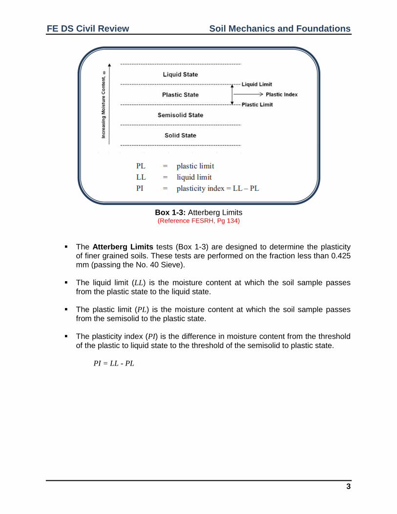
Box 1-3: Atterberg Limits (Reference FESRH, Pg 134)

The Atterberg Limits tests (Box 1-3) are designed to determine the plasticity of finer grained soils. These tests are performed on the fraction less than 0.425 mm (passing the No. 40 Sieve).

The liquid limit (LL) is the moisture content at which the soil sample passes

from the plastic state to the liquid state. The plastic limit (PL) is the moisture content at which the soil sample passes

from the semisolid to the plastic state.

The plasticity index (PI) is the difference in moisture content from the threshold of the plastic to liquid state to the threshold of the semisolid to plastic state.

PI = LL - PL


4

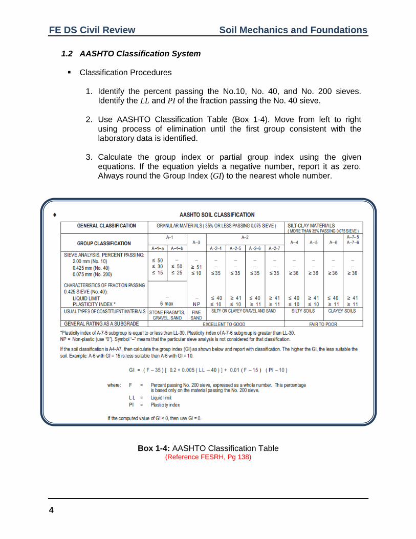
1.2 AASHTO Classification System

Classification Procedures

1. Identify the percent passing the No.10, No. 40, and No. 200 sieves. Identify the LL and PI of the fraction passing the No. 40 sieve.

2. Use AASHTO Classification Table (Box 1-4). Move from left to right using process of elimination until the first group consistent with the laboratory data is identified.

3. Calculate the group index or partial group index using the given

equations. If the equation yields a negative number, report it as zero. Always round the Group Index (GI) to the nearest whole number.

Box 1-4: AASHTO Classification Table (Reference FESRH, Pg 138)


5

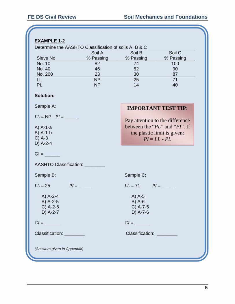
EXAMPLE 1-2

Determine the AASHTO Classification of soils A, B & C

Sieve No

Soil A % Passing

Soil B % Passing

Soil C % Passing

No. 10 82 74 100 No. 40 46 52 90 No. 200 23 30 87

LL NP 25 71 PL NP 14 40

Solution:

Sample A: LL = NP PI = _____ A) A-1-a B) A-1-b C) A-3 D) A-2-4 GI = ______ AASHTO Classification: ________ Sample B: LL = 25 PI = _____

A) A-2-4 B) A-2-5 C) A-2-6 D) A-2-7

GI = ______ Classification: ________

Sample C:

LL = 71 PI = _____

A) A-5 B) A-6 C) A-7-5 D) A-7-6

GI = ______ Classification: ________


IMPORTANT TEST TIP:

Pay attention to the difference

between the “PL” and “PI”. If

the plastic limit is given:

PI = LL - PL


6

1.3 Unified Soil Classification System (USCS)

Group Symbols First Letter: G Gravel S Sand M Silt C Clay Second Letter: For Course-Grained Soils - “G” or “S” P Poorly Graded W Well Graded M Silty C Clayey For Fine-Grained Soils – “M” or “C” L Low Plasticity H High Plasticity or Elastic

Box 1-5: USCS Classification Table (Reference FESRH, Pg 137)


7

Classification Procedures:

1. Identify the percent gravel, percent sand and percent fines (using No. 4 and No. 200 sieves). Note that “fines” refer to soils passing the No. 200 sieve.

2. If the percent passing the No. 200 sieve is less than 50%, then the soil is

“coarse-grained”.

For soils with less than 5% fines, determine Cu & Cc to determine group symbol (GW, GP, SW, or SP).

For soils with greater than 12% fines, determine the LL and PI of

fraction passing the No. 40 sieve and plot results on the Casegrande Plasticity Chart to determine group symbol (GM, GC, SM, or SC). If the fines plot in the “CL-ML” area, the group symbol will either be GC-GM or SC-SM.

3. If the soil has 5 to 12 % fines, the soil will have a dual symbol.

First symbol will be GW, GP, SW, or SP, depending on values of Cu

& Cc. Second symbol will be GM, GC, SM, or SC according to where fines plot on the Casegrande Plasticity Chart. Only the following combinations are possible:

GW-GM SW-SM GW-GC SW-SC GP-GM SP-SM GP-GC SP-SC

4. If the percent passing the No. 200 sieve is greater than or equal to 50%,

then the sample is “fine-grained”.

Determine the LL and PI and plot results on Casagrande Plasticity Chart. Note that “non-plastic” soil (PI < 4) classifies as non-plastic silt (ML).


8

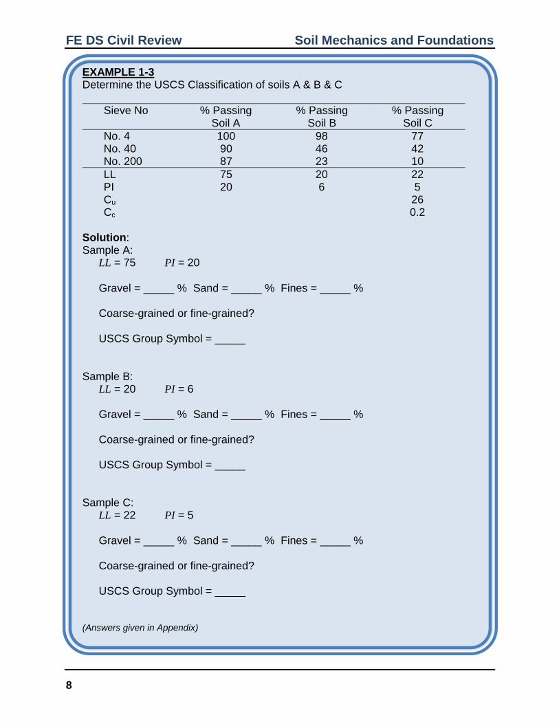
EXAMPLE 1-3 Determine the USCS Classification of soils A & B & C

Sieve No % Passing Soil A

% Passing Soil B

% Passing Soil C

No. 4 100 98 77 No. 40 90 46 42 No. 200 87 23 10

LL 75 20 22 PI 20 6 5 Cu 26 Cc 0.2

Solution: Sample A:

LL = 75 PI = 20 Gravel = _____ % Sand = _____ % Fines = _____ % Coarse-grained or fine-grained? USCS Group Symbol = _____

Sample B:

LL = 20 PI = 6

Gravel = _____ % Sand = _____ % Fines = _____ % Coarse-grained or fine-grained? USCS Group Symbol = _____

Sample C:

LL = 22 PI = 5

Gravel = _____ % Sand = _____ % Fines = _____ % Coarse-grained or fine-grained? USCS Group Symbol = _____



9

2.0 Phase Relationships

Total Volume V = Va + Vw + Vs Total Weight W = Ww + Ws

V = Vv + Vs

Box 2-1: Phase Diagram

Box 2-2: Common Soil Properties (Reference FESRH, Pg 134)


10

Water content (ratio of weights) and saturation (ratio of volumes):

Moisture Content, Weight of Water

100%Weight of Solids

w

s

Ww

W

Degree of Saturation, Volume of Water

100%Volume of Voids

w

v

VS

V

[True or False] The moisture content can be greater than 100%. [True or False] The degree of saturation can be greater than 100%. If the moisture content is 0%, what is the degree of saturation? _____ If the degree of saturation is 100%, what is the moisture content? _____


Unit weight is a generic term to describe a weight per unit volume. The

descriptive terms “total”, “saturated”, “dry”, and “effective” all indicate a specific weight-volume relationship.

Total unit weight: Total Weight

Total Volume

W

V

Saturated unit weight is a special case of total unit weight, when 100% of soil

voids are filled with water (S = 1.0)

( ) ( )Total Weight of Saturated Soil

Total Volume 1 1

sat s w ssat

t

W G e G e

V e w

Dry unit weight: Weight of Solids

Total Volume 1 1

s s wd

W G

V e w

[True or False] If the dry unit weight of a soil is 100 pcf, the moisture content must be 0%. (Answers given in Appendix)


11

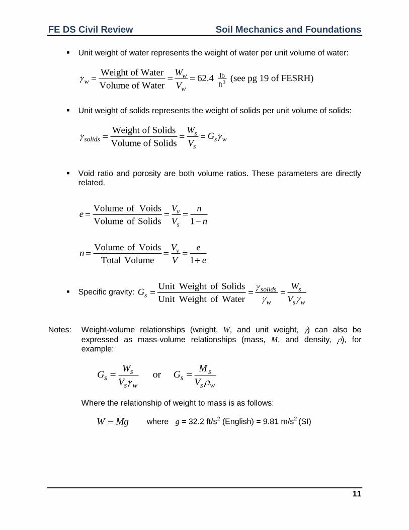
Unit weight of water represents the weight of water per unit volume of water:

3

lb

ft

Weight of Water62.4 (see pg 19 of FESRH)

Volume of Water

ww

w

W

V

Unit weight of solids represents the weight of solids per unit volume of solids:

Weight of Solids

Volume of Solids

ssolids s w

s

WG

V

Void ratio and porosity are both volume ratios. These parameters are directly related.

Volume of Voids

Volume of Solids 1

v

s

V ne

V n

Volume of Voids

Total Volume 1

vV en

V e

Specific gravity: Unit Weight of Solids

Unit Weight of Water

solids ss

w s w

WG

V

Notes: Weight-volume relationships (weight, W, and unit weight, ) can also be

expressed as mass-volume relationships (mass, M, and density, ), for example:

or s ss s

s w s w

W MG G

V V

Where the relationship of weight to mass is as follows:

W Mg where g = 32.2 ft/s2 (English) = 9.81 m/s2 (SI)


12

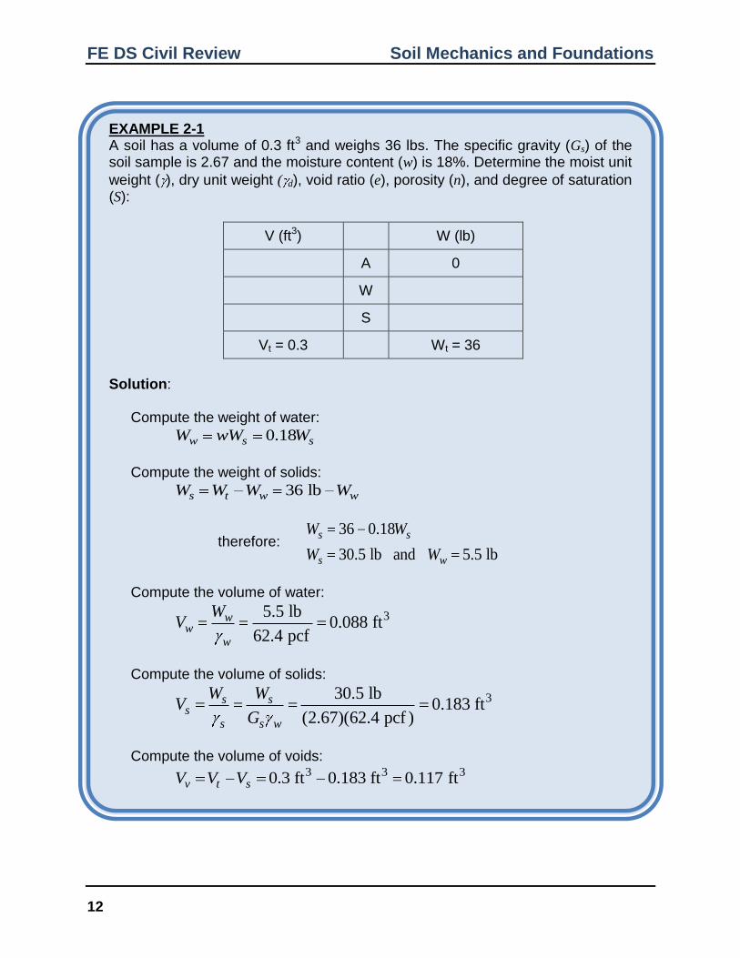
EXAMPLE 2-1 A soil has a volume of 0.3 ft3 and weighs 36 lbs. The specific gravity (Gs) of the soil sample is 2.67 and the moisture content (w) is 18%. Determine the moist unit

weight ( ), dry unit weight ( d), void ratio (e), porosity (n), and degree of saturation (S):

V (ft3) W (lb)

A 0

W

S

Vt = 0.3 Wt = 36

Solution:

Compute the weight of water:

0.18w s sW wW W

Compute the weight of solids:

36 lbs t w wW W W W

therefore: 36 0.18

30.5 lb and 5.5 lb

s s

s w

W W

W W

Compute the volume of water:

35.5 lb

0.088 ft62.4 pcf

ww

w

WV

Compute the volume of solids:

330.5 lb

0.183 ft(2.67)(62.4 pcf )

s ss

s s w

W WV

G

Compute the volume of voids:

3 3 30.3 ft 0.183 ft 0.117 ftv t sV V V


13

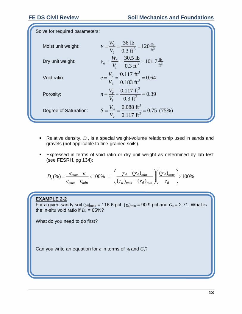
Solve for required parameters:

Moist unit weight: 3

lb3 ft

36 lb120

0.3 ft

t

t

W

V

Dry unit weight: 3

lb3 ft

30.5 lb101.7

0.3 ft

sd

t

W

V

Void ratio:

3

3

0.117 ft0.64

0.183 ft

v

s

Ve

V

Porosity:

3

3

0.117 ft0.39

0.3 ft

v

t

Vn

V

Degree of Saturation:

3

3

0.088 ft0.75 (75%)

0.117 ft

w

v

VS

V

Relative density, Dr, is a special weight-volume relationship used in sands and

gravels (not applicable to fine-grained soils). Expressed in terms of void ratio or dry unit weight as determined by lab test

(see FESRH, pg 134):

( ) ( )(%) 100% 100%

( ) ( )

max d d min d maxr

max min d max d min d

e eD

e e

EXAMPLE 2-2

For a given sandy soil ( d)max = 116.6 pcf, ( d)min = 90.9 pcf and Gs = 2.71. What is the in-situ void ratio if Dr = 65%? What do you need to do first?

Can you write an equation for e in terms of d and Gs?


14

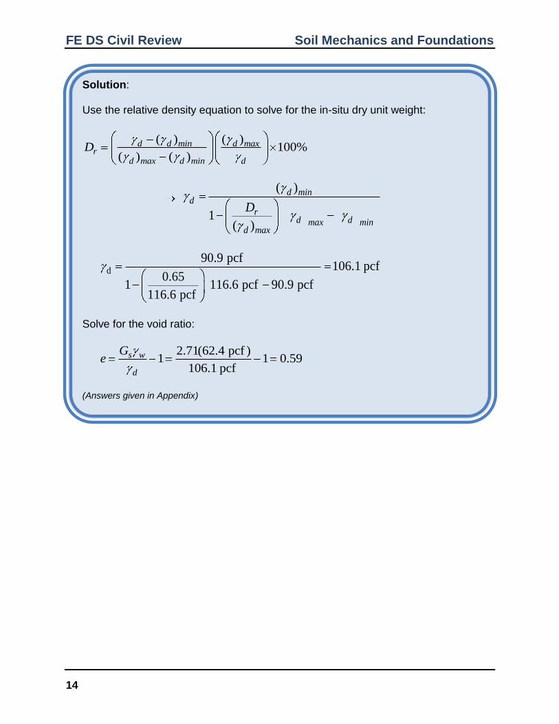
Solution: Use the relative density equation to solve for the in-situ dry unit weight:

( ) ( )100%

( ) ( )

d d min d maxr

d max d min d

D

( )

1( )

d mind

rd dmax min

d max

D

d

90.9 pcf106.1 pcf

0.651 116.6 pcf 90.9 pcf

116.6 pcf

Solve for the void ratio:

2.71(62.4 pcf )

1 1 0.59106.1 pcf

s w

d

Ge



15

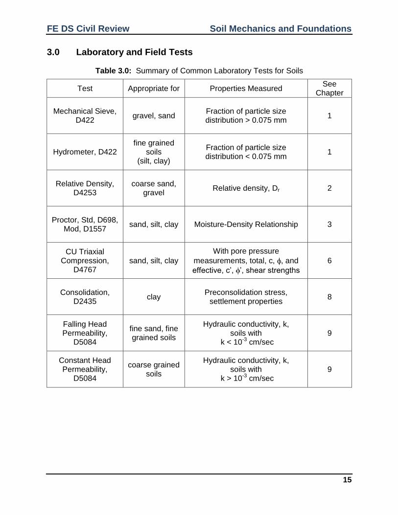
3.0 Laboratory and Field Tests

Table 3.0: Summary of Common Laboratory Tests for Soils

Test Appropriate for Properties Measured See

Chapter

Mechanical Sieve, D422

gravel, sand Fraction of particle size distribution > 0.075 mm

1

Hydrometer, D422 fine grained

soils (silt, clay)

Fraction of particle size distribution < 0.075 mm

1

Relative Density, D4253

coarse sand, gravel

Relative density, Dr 2

Proctor, Std, D698, Mod, D1557

sand, silt, clay Moisture-Density Relationship 3

CU Triaxial Compression,

D4767 sand, silt, clay

With pore pressure

measurements, total, c, , and

effective, c’, ’, shear strengths

6

Consolidation, D2435

clay Preconsolidation stress,

settlement properties 8

Falling Head Permeability,

D5084

fine sand, fine grained soils

Hydraulic conductivity, k, soils with

k < 10-3 cm/sec 9

Constant Head Permeability,

D5084

coarse grained soils

Hydraulic conductivity, k, soils with

k > 10-3 cm/sec 9


16

3.1 Proctor Laboratory Tests

Compaction is densification of soil by the reduction of air in the soil voids. The degree of compaction is measured in dry unit weight (dry density).

Standard Proctor Test (ASTM D698) and Modified Proctor Test (ASTM D1557)

Proctor curve cannot plot above the “zero voids” line, which is a plot of dry unit

weight ( d) vs. moisture content (w), at 100 percent saturation (S=100%).

Box 3-1: A typical compaction test proctor curve


17

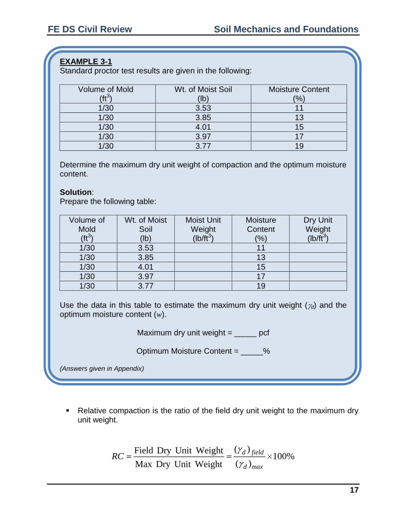
EXAMPLE 3-1 Standard proctor test results are given in the following:

Volume of Mold (ft3)

Wt. of Moist Soil (lb)

Moisture Content (%)

1/30 3.53 11

1/30 3.85 13

1/30 4.01 15

1/30 3.97 17

1/30 3.77 19

Determine the maximum dry unit weight of compaction and the optimum moisture content. Solution: Prepare the following table:



Moist Unit Weight (lb/ft3)

Moisture Content

(%)

Dry Unit Weight (lb/ft3)

1/30 3.53 11

1/30 3.85 13

1/30 4.01 15

1/30 3.97 17

1/30 3.77 19

Use the data in this table to estimate the maximum dry unit weight ( d) and the optimum moisture content (w).

Maximum dry unit weight = _____ pcf

Optimum Moisture Content = _____%


Relative compaction is the ratio of the field dry unit weight to the maximum dry unit weight.

( )Field Dry Unit Weight100%

( )Max Dry Unit Weight

d field

d max

RC


18

4.0 Vertical Total and Effective Stress

Box 4-1: Vertical Stress Parameters (Reference FESRH, pg 135)

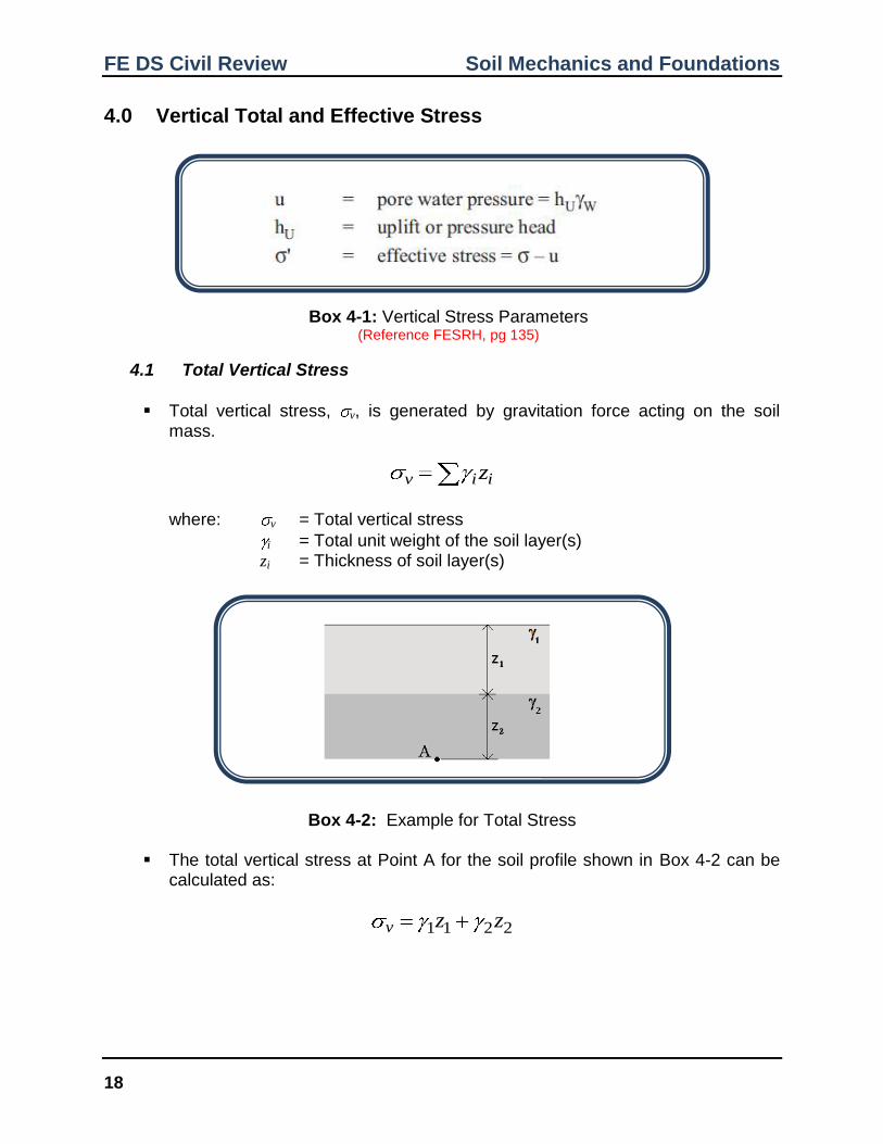
4.1 Total Vertical Stress

Total vertical stress, v, is generated by gravitation force acting on the soil mass.

v i iz

where: v = Total vertical stress

i = Total unit weight of the soil layer(s) zi = Thickness of soil layer(s)

Box 4-2: Example for Total Stress

The total vertical stress at Point A for the soil profile shown in Box 4-2 can be calculated as:

1 1 2 2v z z


19

4.2 Pore Water Pressure

Pore water pressure is the result of buoyant force, u, exerted by water in the soil mass.

CASE 1: Pore water pressure in hydrostatic conditions (no flow). Use this case by default unless otherwise specified.

w wu z

where: u = Pore water pressure

w = Unit weight of water hu = zw = Depth below the groundwater surface

(for no flow = phreatic surface)

CASE 2: Pore water pressure in seepage conditions (1-D upward or downward flow).

w pu h

where: u = Pore water pressure

w = Unit weight of water hu = hp = Pressure (piezometric) head at the point of interest

Box 4-3: Case 1 (hydrostatic conditions with no flow) and Case 2 (seepage conditions)


20

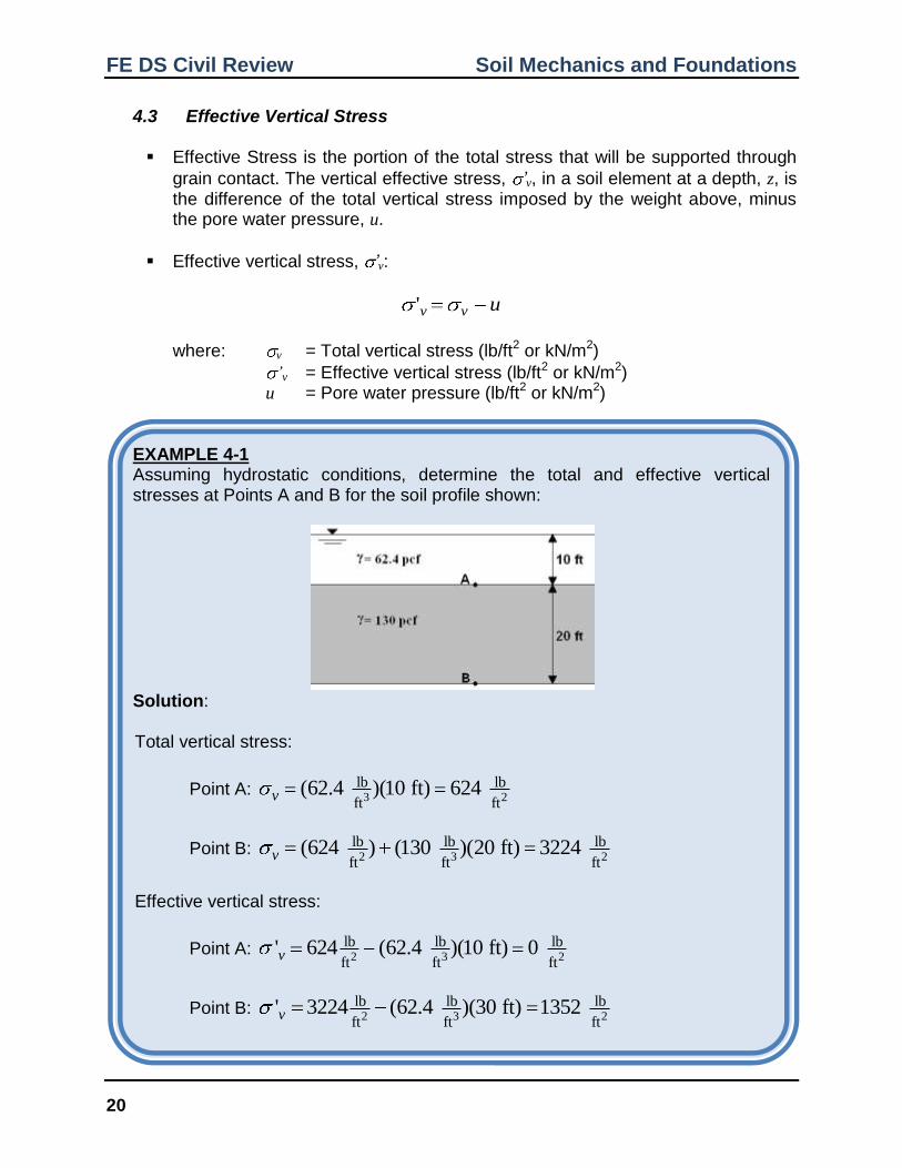
4.3 Effective Vertical Stress

Effective Stress is the portion of the total stress that will be supported through

grain contact. The vertical effective stress, ’v, in a soil element at a depth, z, is the difference of the total vertical stress imposed by the weight above, minus the pore water pressure, u.

Effective vertical stress, ’v:

uvv'

where: v = Total vertical stress (lb/ft2 or kN/m2)

’v = Effective vertical stress (lb/ft2 or kN/m2) u = Pore water pressure (lb/ft2 or kN/m2)

EXAMPLE 4-1 Assuming hydrostatic conditions, determine the total and effective vertical stresses at Points A and B for the soil profile shown:

Solution: Total vertical stress:

Point A: 3 2

lb lb

ft ft(62.4 )(10 ft) 624 v

Point B: 2 3 2

lb lb lb

ft ft ft(624 ) (130 )(20 ft) 3224 v

Effective vertical stress:

Point A: 2 3 2

lb lb lb

ft ft ft' 624 (62.4 )(10 ft) 0 v

Point B: 2 3 2

lb lb lb

ft ft ft' 3224 (62.4 )(30 ft) 1352 v


21

5.0 Retaining Walls

5.1 Earth Pressure Introduction

Earth pressure is the force per unit area exerted by soil. The ratio of horizontal to vertical stress is called coefficient of lateral earth pressure (K).

' and

'

h h

v v

K K

Earth pressure forces can be at-rest (a), active (b) or passive (c).

Box 5-1: Nature of Lateral Earth Pressure on a Retaining Wall (Source: Das, 2007)

5.2 Rankine Earth Pressure Theory

For level backfill ( = 0):

2tan (45 )2

AK and 2tan (45 )

2PK

The total active resultant force (where = 0) is solved for by:

21 1

2 2A A AP p H K H

The total passive resultant force (where = 0) is solved for by:

21 1

2 2p p pP p H K H


22

EXAMPLE 5-1

A 10 ft high gravity retaining wall with flat backfill ( = 0) retains a clean sand for

which = 120 lb/ft3 and = 32 . Using Rankine’s earth pressure theory, calculate the total active earth pressure, and the active resultant force.

Solution: Calculate the active earth pressure coefficient:

2 2 32

2 2tan (45 ) tan (45 ) 0.307AK

Calculate the active earth pressure and resultant force:

(120 pcf )(10 ft)(0.307) 368 psfA Ap HK

1 1

(368 psf )(10 ft) 1842 plf2 2

A AP p H


23

EXAMPLE 5-2

The sandy soil with an internal angle of friction of 30 degrees is retained behind a 9-foot retaining wall has moist unit weight of 128 pcf. Due to poor drainage, the water table has risen to 6 feet above the base of the wall. The saturated unit weight of the soil is 135 pcf. What is the total active resultant force acting on the wall?

Solution: Determine the resultant active earth force, Pa:

2 30tan (45 ) 0.333

2AK

1 2 3A A A A WP P P P P

11 1 12

0.5 (0.333)(3 ft)(128 pcf ) (3 ft) 191.8 plfA AP K H H

2 1 2 (0.333)(3 ft)(128 pcf ) (6 ft) 767.2 plfA AP K H H

1

3 2 22' 0.5 (0.333)(6 ft)(135 pcf - 62.4 pcf ) (6 ft) 435.2 plfA AP K H H

12 22

0.5 (6 ft)(62.4 pcf ) (6 ft) 1123.2 plfW wP H H

191.8 767.3 435.2 1123.2 2517.5 plfAP


24

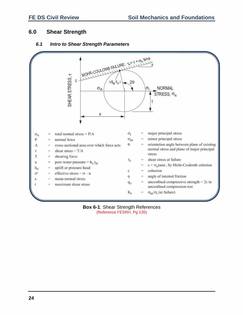
6.0 Shear Strength

6.1 Intro to Shear Strength Parameters

Box 6-1: Shear Strength References (Reference FESRH, Pg 135)


25

EXAMPLE 6-1 A triaxial test is performed on a soil sample consisting of dry sand. Failure occurred at a normal stress of 6,260 psf and a shear stress was 4,175 psf. Determine the internal angle of friction and the major and minor principal stresses.

Solution: Compute the internal angle of friction:

When c = 0, 1 1 4175 psf

tan tan 346260 psf

F

N

Solve for I and III by writing two equations using the geometry of the Mohr’s circle and shear strength plot:

2( ) 2(4175 psf)cos 10,072 psf

cos(34 )2

F F FI III

I III I IIIt

2sin +3.49 28,122 psf

2

I IIIN

I III NNI III

I III I III

s

t

By solving simultaneously: 14,092 psf and 4,020 psf I III


26

7.0 Shallow Spread Foundations

7.1 Types of Foundations

Foundations can be classified as shallow or deep:

(a) Shallow: spread footings and mats (b) Deep: Driven piles, drilled shafts, and piers

For shallow foundation, depth is shallower than its width.

For deep foundation, depth (Df) is larger than its width (B). Generally, deep

foundations have the ratio (10 Df /B).

7.2 General Bearing Capacity Theory

The ultimate bearing capacity is theoretically the bearing pressure at which shear failure will occur.

Terzaghi’s general bearing capacity equation is given as:

0.5q cN D N BNult c f q

where: qult = Ultimate bearing capacity c = cohesion Df = Depth of footing

= Unit weight of the soil B = Width or diameter of footing

Nc, Nq, N = Bearing capacity factors based on The allowable bearing capacity is the maximum bearing pressure the soil can

safely support with a reasonable factor of safety (typically 2 to 3 for foundations):

q

qultq

all FS

Note that bearing capacity and bearing pressure can be thought of in terms of

“supply” and “demand”. The allowable bearing capacity is the available supply, which must be greater than or equal to the applied bearing pressure, which is the demand placed on the soil.

all appliedq Q


27

EXAMPLE 7-1 Determine the ultimate and allowable bearing capacities for a continuous footing with a width of 3.5 feet. The foundation is bearing 2 feet below the ground surface in sand with unit weight of 130 psf, and an internal angle of friction of 36 degrees (c = 0). Assume a factor of safety of 3.0.

Solution:

Determine bearing capacity factors:

Nc = 50, N = 56, Nq = 38

1) Solve for the ultimate bearing capacity.

0.5ult c f qq cN D N BN

2 3 3

lb lb lb

ft ft ft(0 )(50) (130 )(2 ft)(38) 0.5(130 )(3.5 ft)(56) 22,620 psfultq

2) Solve for the allowable bearing capacity.

22,620 psf7,540 psf

3

ultall

qq

FS

EXAMPLE 7-2 Determine the factor of safety for a continuous footing with a width of 3.5 feet carrying a load of 18 kips per lineal foot (plf). The foundation is bearing 2 feet below the ground surface in sand with unit weight of 130 psf, and an internal angle of friction of 36 degrees (c = 0).

Solution: 1) Solve for the ultimate bearing capacity (from previous solution)

2 3 3

lb lb lb

ft ft ft(0 )(50) (130 )(2 ft)(38) 0.5(130 )(3.5 ft)(56) 22,620 psfultq

2) Solve for the bearing pressure.

18,000 lb9000 psf

2 ft 1 ft

PQ

A

3) Solve for FSq.

22,620 psf2.5

9,000 psf

ultq

qFS

Q


28

8.0 Consolidation 8.1 Load Distribution in Soils

EXAMPLE 8-1 A point load with a magnitude of 180,000 lbs acts at the ground surface. Determine the vertical stress increase due to the applied point load at a vertical distance of 10 feet, and depth of 20 feet from the point of application. Solution: (Reference FESRH, pg 139)

For uniformly loaded circular and rectangular areas, the increase in vertical stress is determined by:

s zp q I

where: qs = Applied bearing pressure Iz = Influence factor

and: load

areasq

EXAMPLE 8-2 A flexible rectangular area measures 10 by 20 ft in plan. It supports an applied pressure of 3,000 psf. Determine the vertical stress increase due to the applied load at a depth of 20 ft below the corner of the rectangular area. Solution: (Reference FESRH, pg 140)

( )(3000 psf ) 360 psfIq


2 2

10 ft0.5 0.2733

20 ft

180,000 lbs(0.2733) 123 psf

(20 ft)

r

r

rC

z

Pp C

z

10 ft 20 ft0.5 1.0

20 ft 20 ft

B Lm n I

z z


29

EXAMPLE 8-3 A cylindrical concrete tank has an outer diameter of 80 feet and a height of 40 feet. The concrete is 24 inches thick along the walls and base. The tank is designed to hold water with a maximum depth of 35 feet. Determine the maximum increase in vertical stress (psf) induced by the tank at a depth of 20 feet (Point A) and 40 feet (Point B) below the base of the tank. Solution: Find the volume of concrete and volume of water:

2 2 3

480 ft 40 ft 76 ft 38 ft 28,676 ftconc OD IDV V V

2 3

4(76 ft) (35 ft) 158,776 ftwV

Determine applied bearing pressure:

3 3

2

3 3lb lb

ft ft lb2 ft

4

150 28,676 ft 62.4 158,776 ft2827

80 ft

conc conc w wV Vq

A

q

Determine p at Point A: Note the maximum increase in stress will occur at the center of the loaded area. (See FESRH, pg139)

20 ft 0 ft

0.5 040 ft 40 ft

z

z rI

R R

( )(2827 psf ) 2587 psfA z sp I q

Determine at Point B:

40 ft 0 ft

1.0 040 ft 40 ft

z

z rI

R R

( )(2827 psf ) 1826 psfB z sp I q



30

8.2 Consolidation in Clay Soils

Settlement of fine-grained soils occurs in three stages. Immediate settlement occurs rapidly and is based on the theory of elasticity. Primary consolidation occurs due the extrusion of water from soil pores. Secondary compression (aka “creep”) occurs as soil particles readjust and compress.

Box 8-1: Three phases of settlement in fine-grained soils

(Source: Lui and Evett 2005)

The stress history of soils is summarized by:

For normally consolidated soils: 0 cp p

For overconsolidated soils: 0 cp p

where: po = Initial (present) effective overburden pressure

pc = Preconsolidation pressure


31

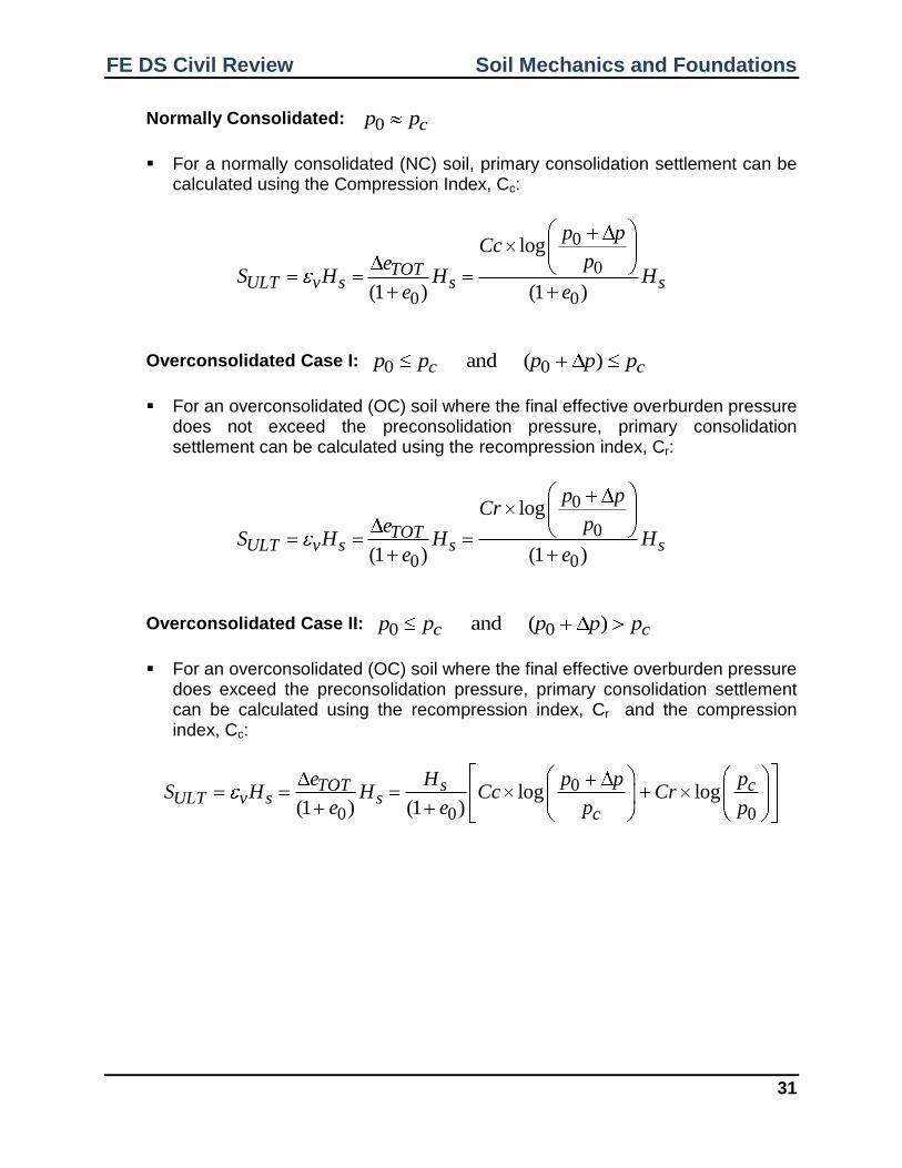
Normally Consolidated: 0 cp p

For a normally consolidated (NC) soil, primary consolidation settlement can be

calculated using the Compression Index, Cc:

0

0

0 0

log

(1 ) (1 )

TOTULT v s s s

p pCc

peS H H H

e e

Overconsolidated Case I: 0 0 and ( )c cp p p p p

For an overconsolidated (OC) soil where the final effective overburden pressure

does not exceed the preconsolidation pressure, primary consolidation settlement can be calculated using the recompression index, Cr:

0

0

0 0

log

(1 ) (1 )

TOTULT v s s s

p pCr

peS H H H

e e

Overconsolidated Case II: 0 0 and ( )c cp p p p p

For an overconsolidated (OC) soil where the final effective overburden pressure

does exceed the preconsolidation pressure, primary consolidation settlement can be calculated using the recompression index, Cr and the compression index, Cc:

0

0 0 0

log log(1 ) (1 )

TOT s cULT v s s

c

e H p p pS H H Cc Cr

e e p p


32

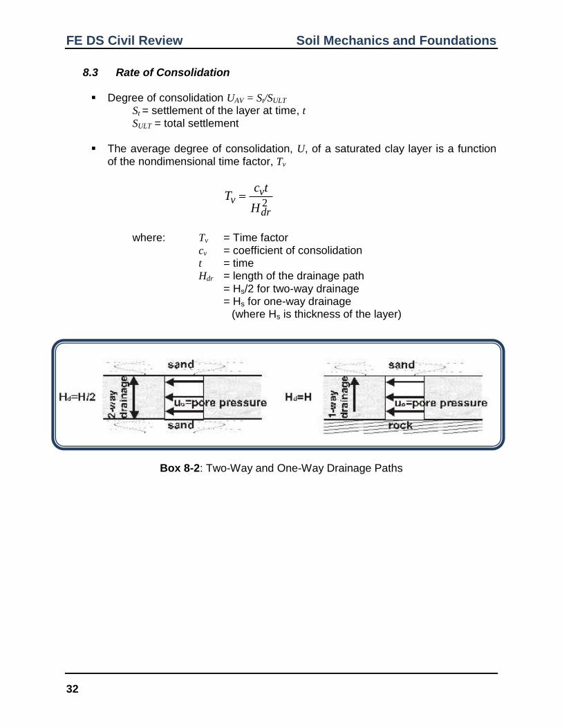
8.3 Rate of Consolidation

Degree of consolidation UAV = St/SULT St = settlement of the layer at time, t SULT = total settlement

The average degree of consolidation, U, of a saturated clay layer is a function of the nondimensional time factor, Tv

where: Tv = Time factor cv = coefficient of consolidation

t = time Hdr = length of the drainage path = Hs/2 for two-way drainage = Hs for one-way drainage (where Hs is thickness of the layer)

Box 8-2: Two-Way and One-Way Drainage Paths

2v

vdr

c tT

H


33

EXAMPLE 8-4

A 15-ft thick clay is bounded by sand at the top and bottom. The clay has a coefficient of consolidation of 0.3 ft2/day. Determine the time when 50% and 90% of the total settlement will occur.

Solution:

Double drainage Hdr = _______

From Table FESRH, pg 141: For U = 50% Tv = ____

For U = 90% Tv = ____ Calculate the time for 50% and 90 % of consolidation to occur:

2

2 2

50ftday

(____)(7.5 ft)37 days

0.3

v d

v

T Ht

c

2

2 2

90ftday

(____)(7.5 ft)159 days

0.3

v d

v

T Ht

c



34

9.0 Permeability & Seepage

9.1 Coefficient of Permeability Laboratory Tests

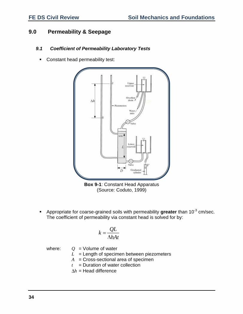
Constant head permeability test:

Box 9-1: Constant Head Apparatus (Source: Coduto, 1999)

Appropriate for coarse-grained soils with permeability greater than 10-3 cm/sec. The coefficient of permeability via constant head is solved for by:

QLk

hAt

where: Q = Volume of water

L = Length of specimen between piezometers A = Cross-sectional area of specimen t = Duration of water collection

h = Head difference


35

EXAMPLE 9-1 A constant-head permeability test was performed on a 110 mm diameter, 270 mm tall fine sand sample in a permeameter similar to the one shown in Box 9-3. The piezometers are spaced 200 mm apart and had readings of 1809 and 1578 mm. The graduated cylinder collected 910 ml of water over 25 min 15 sec. Calculate the hydraulic conductivity of the soil in cm/sec. Solution: Define the following parameters:

3

2 2

4

910 ml 910 cm

(11 cm) 95 cm

20 cm

180.9 cm 157.8 cm 23.1 cm

1515 sec

Q

A

L

h

t

Solve for k:

3

3 cmsec2

(910 cm )(20 cm)5.5 10

(23.1 cm)(95 cm )(1515 s)

QLk

hAt

Falling head permeability test:

Appropriate for fine-grained soils with permeability less than 10-3 cm/sec. The coefficient of permeability via falling head is solved for by:

010

1

2.303 loghaL

kAt h

where: h0 = Head at the start of the test (t0) h1 = Head at the end of the test (t1) L = Length of specimen A = Cross-sectional area of specimen a = Cross-sectional area of standpipe t = Duration of water collection (t1-t0)


36

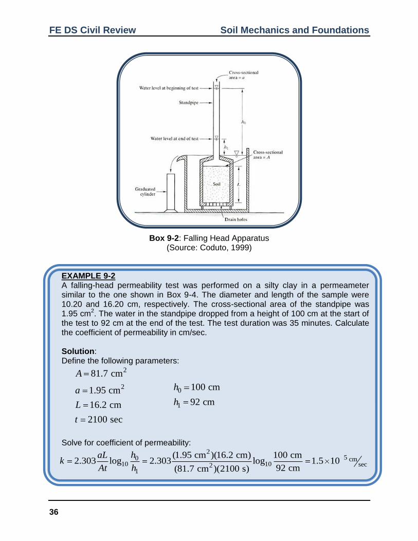
Box 9-2: Falling Head Apparatus (Source: Coduto, 1999)

EXAMPLE 9-2 A falling-head permeability test was performed on a silty clay in a permeameter similar to the one shown in Box 9-4. The diameter and length of the sample were 10.20 and 16.20 cm, respectively. The cross-sectional area of the standpipe was 1.95 cm2. The water in the standpipe dropped from a height of 100 cm at the start of the test to 92 cm at the end of the test. The test duration was 35 minutes. Calculate the coefficient of permeability in cm/sec. Solution: Define the following parameters:

2

2

81.7 cm

1.95 cm

16.2 cm

2100 sec

A

a

L

t

0

1

100 cm

92 cm

h

h

Solve for coefficient of permeability: 2

50 cm10 10 sec2

1

(1.95 cm )(16.2 cm) 100 cm2.303 log 2.303 log 1.5 10

92 cm(81.7 cm )(2100 s)

haLk

At h


37

9.2 Flow Nets

Laplace’s Equation represents energy loss through a resistive medium (i.e. flow through soil). A flow net is a 2D graphical solution of Laplace’s Equation.

A flow net is a combination of flow lines and equipotential lines. A flow line is a line along which a water particle travels. There is no flow along equipotential lines, which are 90 degrees to flow lines.

The total head along an equipotential line is equal at all points. The total flow rate (per unit width) though a flow net, is solved for by:

f

d

NQ k h

N

where: Q = Total flow rate Nf = Number of flow channels in a flow net Nd = Number of potential drops

h = Head change from upstream to downstream k = Coefficient of permeability


38

EXAMPLE 9-3 For a flow net shown in the following figure, determine head loss at points A, B, and C. The structure is approximately 100 feet long. Determine the flow rate in ft3/min

through the permeable layer. Assume hydraulic conductivity, k = 1.64 10-4 ft/min.

.

Solution: Nf = ____ Nd = ____ Total head loss (H) = ____ Head loss per drop = ____ Head loss at Pnt A = ____ Pnt B = ____ Pnt C = ____ Calculate seepage:

3ft__________

min

f

d

NQ kH L

N


APPENDIX

Example 1-1

D60 6 mm, D30 0.3 mm, D10 0.08 mm

60

10

6mm75

0.08mmu

DC

D;

2 230

60 10

(0.3mm)0.1875

(6mm)(0.08mm)z

DC

D D

Example 1-2 Sample A PI = NP Classification: A-1-b Sample B PI = 11 Classification: A-2-6 Sample C PI = 31

(87 35)[0.2 0.005(71 40)] 0.01(87 15)(31 10) 33.58GI

Classification: A-7-5 (34)

6 mm 0.08 mm 0.3 mm

APPENDIX

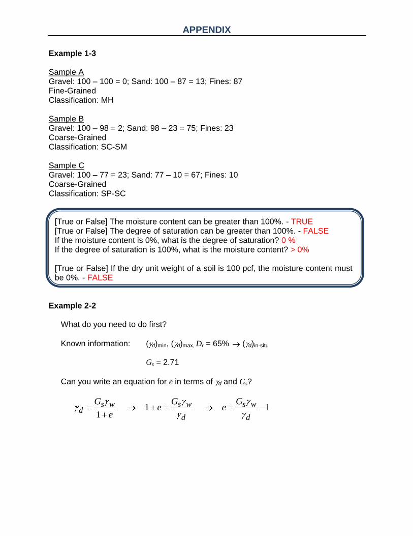
Example 1-3 Sample A Gravel: 100 – 100 = 0; Sand: 100 – 87 = 13; Fines: 87 Fine-Grained Classification: MH Sample B Gravel: 100 – 98 = 2; Sand: 98 – 23 = 75; Fines: 23 Coarse-Grained Classification: SC-SM Sample C Gravel: 100 – 77 = 23; Sand: 77 – 10 = 67; Fines: 10 Coarse-Grained Classification: SP-SC

[True or False] The moisture content can be greater than 100%. - TRUE [True or False] The degree of saturation can be greater than 100%. - FALSE If the moisture content is 0%, what is the degree of saturation? 0 % If the degree of saturation is 100%, what is the moisture content? > 0% [True or False] If the dry unit weight of a soil is 100 pcf, the moisture content must be 0%. - FALSE

Example 2-2

What do you need to do first?

Known information: ( d)min, ( d)max, Dr = 65% ( d)in-situ

Gs = 2.71

Can you write an equation for e in terms of d and Gs?

1 11

s w s w s wd

d d

G G Ge e

e

APPENDIX

Example 3-1



Moist Unit Weight (lb/ft3)

Moisture Content

(%)

Dry Unit Weight (lb/ft3)

1/30 3.53 105.9 11 95.4

1/30 3.85 115.5 13 102.2

1/30 4.01 120.3 15 104.6

1/30 3.97 119.1 17 101.8

1/30 3.77 113.1 19 95.0

Maximum dry unit weight = 105 pcf; Optimum Moisture Content = 15 % Example 8-2

(1.20)(3000 psf ) 360 psfIq

Example 8-3

(0.915)(2827 psf ) 2587 psfA z sp I q

(0.645)(2827 psf ) 1826 psfB z sp I q

Example 8-4

Double drainage Hdr = (15ft/2) = 7.5 ft

2

2 2

50ftday

(0.196)(7.5 ft)37 days

0.3

v d

v

T Ht

c;

2

2 2

90ftday

(0.848)(7.5 ft)159 days

0.3

v d

v

T Ht

c

Example 9-3

Nf = 4; Nd = 8; Total head loss (H) = (20 ft – 8 ft) = 12 ft;

Head loss per drop = (12 ft/8 drops) = 1.5 ft/drop

Head loss at Pnt A = (1.5ft/drop) x 2 drops = 3 ft Head loss at Pnt B = Pnt C = (1.5ft/drop) x 5 drops = 7.5 ft

34 ft

min

4 ft(1.64 10 )(12ft) (100ft) 0.0984

8 min

f

d

NQ kH L

N

civil depth notes for mar 15th-soil

Documents