civil service rules and policy choices: evidence from us state … · 2015-01-06 · civil service...
TRANSCRIPT

338
American Economic Journal: Economic Policy 2014, 6(2): 338–380 http://dx.doi.org/10.1257/pol.6.2.338
Civil Service Rules and Policy Choices: Evidence from US State Governments†
By Gergely Ujhelyi*
This paper studies the policy impact of civil service regulations, exploiting reforms undertaken by US state governments throughout the twentieth century. These reforms replaced political patronage with a civil service recruited based on merit and protected from politics. I find that state politicians respond to these changes by spending relatively less through the reformed state-level bureaucracies. Instead, they allocate more funds to lower level governments. The reallocation of expenditures leads to reduced long-term investment by state governments. (JEL D73, H72, H77, H79)
Does a professional, independent bureaucracy lead to better governance? A distinguished tradition going back to at least Max Weber has argued that the
answer is “yes,” and viewed the alternative political patronage as a source of cor-ruption, waste, and the dominance of special interests. Today, the institution of a civil service with competitive, merit-based recruitment and protection from political pressure is a defining characteristic of modern democracies, and reform towards this ideal is advocated for developing countries by the World Bank and other organiza-tions.1 At the same time, the precise extent of civil service protections, including tenure and other rights of public employees, has been a contentious question and this is an active area of institutional reform in several developed countries. In the United States, recent legislation in Georgia (1996), Florida (2001), and Arizona (2012) ended traditional civil service protections for a substantial number of state workers, while measures in Washington (2002) and Idaho (2011) increased manag-ers’ flexibility to promote or fire employees. This paper studies the effect of civil service regulations on the policy choices of politicians.
1 According to the United Nations Development Programme (UNDP), “it is generally agreed that a compe-tent civil service has the following characteristics: it is merit-based and politically neutral...” (United Nations Development Programme (UNDP) 2001, 5). Between 1981 and 1991, civil service reforms were a component in 90 World Bank loans to 44 different countries totalling over $4.6 billion (Lindauer and Nunberg 1996).
* Department of Economics, University of Houston, 204 McElhinney Hall, Houston, TX, 77204 (e-mail: [email protected]). I thank seminar participants at the National Bureau of Economic Research Political Economy meeting and the 2013 Public Choice Society conference, as well as Aimee Chin, Steve Craig, Chinhui Juhn, Andrea Szabó, three anonymous referees, and especially Brian Knight for useful comments and suggestions. I also thank David Bostashvili for outstanding research assistance, Sophia Kazinnik and Ben Thompson for help in early stages of the data collection, and Jennifer Burnett from the Council of State Governments for assistance with the Book of the States data. Thanks to Fernando Ferreira and Joseph Gyourko for sharing their data on city mayors. Financial support from the W. E. Upjohn Institute for Employment Research is gratefully acknowledged. The usual disclaimers apply.
† Go to http://dx.doi.org/10.1257/pol.6.2.338 to visit the article page for additional materials and author disclosure statement(s) or to comment in the online discussion forum.

VoL. 6 No. 2 339ujhelyi: Civil ServiCe ruleS and PoliCy ChoiCeS
The institutional debate on civil service regulations tends to focus on bureaucrats. Merit-based recruitment and civil service protections were originally introduced to increase bureaucratic competence, and recent steps to dismantle some of these pro-tections aim at increasing bureaucratic efficiency and reducing red tape. This reflects the traditional view that “The field of administration is a field of business. It is removed from the hurry and strife of politics.” (Wilson 1887, 209). But changes in the way bureaucrats operate are likely to also affect politicians’ choices, and there-fore the policies that bureaucrats may be asked to implement. Civil service regu-lations can impact the distribution of expenditures across government programs. Welfare programs may become less attractive to politicians if checks will be distrib-uted by career civil servants rather than by loyal patronage employees; large con-struction projects may become less attractive when bureaucrats cannot be influenced to award the contract to a bidder favored by the politician or to locate the project in a swing district. Regulations can also impact the distribution of expenditures across government agencies. Politicians may circumvent a bureaucracy that has become less responsive to their demands by directing spending through other government agencies or lower level governments. Understanding politicians’ response to civil service regulations is a crucial step in assessing their welfare implications.
In this paper, I study the impact of civil service regulations on policy choices using new data on the timing of bureaucratic reforms in US state governments. The Pendleton Act of 1883 is generally credited with introducing the merit system in US (federal) government and making the recruitment and day-to-day operation of bureaucracies free from politics.2 The two key provisions of the Act established the principle of merit-based recruitment (competitive examinations) and prohibited the firing or demotion of employees for political reasons. Similar merit systems were gradually adopted by state governments throughout the twentieth century. These reforms were typically the result of voter demands for good government and, once adopted, would remain in place for the foreseeable future, often engraved in states’ constitution. As such, they created a new set of institutional constraints for state politicians. I collected original data on the dates each state adopted the merit sys-tem as well as various details of the regulations. I use this data to study changes in state governments’ spending patterns following bureaucratic reform in the period 1942–1983.
I find that states introducing the merit system channel less spending through their reformed bureaucracies. Instead, they significantly increase the funds transferred to lower level governments, which are typically not constrained by state-level merit systems. This is true both for overall spending, and for politically salient categories such as welfare expenditures and roads. Once the state-level bureaucracy becomes professionalized and independent, state governments shift some of their expendi-tures in these areas to lower level governments. These patterns are consistent with politicians rationally substituting away from ways of spending money over which they have less control.
2 The introduction of the merit system represented a shift towards the Weberian ideal, away from the system of political patronage which it replaced. The consensus among public administration scholars and practitioners is that, at the time, this resulted in considerable improvement in the functioning of bureaucracies.
340 AmErIcAN EcoNomIc JoUrNAL: EcoNomIc PoLIcy mAy 2014
The findings are reinforced when looking at the details of state-level regulations. Merit systems differ in the degree of control awarded to the state governor: states that require the chief personnel executive to be selected by an independent civil service board allow the least control. One might expect governors in such states to have increased incentives to rely on lower level governments in the administration of state projects. Indeed, I find that lower gubernatorial control, as measured by the independence of the personnel executive, leads to larger increases in intergovern-mental transfers.
Does the reallocation of spending across units of government affect the level of expenditures in the affected categories? The evidence shows that it does. I find that introducing the merit system leads to lower spending on investments in roads and other long-term capital projects. All these findings are robust to controlling for a number of factors, including the strength of political parties and a measure of voter ideology, which may simultaneously affect institutional reform and spending patterns.
While my quantitative findings are specific to the context and period being stud-ied, the results have a number of general implications. These provide potentially important considerations for current civil service reform proposals in the United States and elsewhere. First, my results emphasize the need to understand the impact of bureaucratic reform in the context of the entire policy process. This includes not just policy implementation by the bureaucracy, but also the policy choices of elected politicians. Politicians’ response to reform could either reinforce or offset any direct benefits from the merit system or other improvements of the bureaucracy. Second, I show that lowering politicians’ control over bureaucrats in higher level governments can lead to the redistribution of spending towards lower levels of decision making. Moving resources away from the reformed bureaucracy in this way could be socially undesirable.3 The policy implication is that reforming multiple levels of government simultaneously could be more desirable than a gradual approach that focuses on specific levels. Third, my results point to a potentially important political economy motive behind decentralization. As the UNDP notes, “in most countries in which the [national] civil service is charged with making and implementing policy, pres-sures for decentralization and deconcentration are mounting” (UNDP 2001, 32). The results in this paper suggest that some of this pressure could be the result of politicians seeking to maximize their rents while being constrained by civil service regulations at the national level.
In the remainder of the paper, Section I places this paper in the related literature, Section II describes the background and presents the merit system data, Section III describes the theoretical framework, Section IV discusses the empirical strategy, Sections V and VI present the results, and Section VII concludes.
3 In the concluding section, I discuss the assumptions that are needed to draw normative lessons on the desir-ability of civil service reform from my analysis.

VoL. 6 No. 2 341ujhelyi: Civil ServiCe ruleS and PoliCy ChoiCeS
I. Related Literature
A large literature now studies how institutions shape the behavior of policymak-ers (see Besley and Case 2003 for a survey in the context of US states). While electoral rules (e.g., rules on voter registration, primaries, or campaign finance) and decision-making rules (e.g., super-majority requirements or governors’ veto pow-ers) have received considerable attention, there is much less work on the effect of bureaucratic rules.4
Most previous research does not study the rules governing existing bureaucracies, but rather asks whether it is desirable to have an elected politician or an appointed bureaucrat in the first place (Besley and Coate 2003; Alesina and Tabellini 2007; Coate and Knight 2011; Vlaicu and Whalley 2011; Whalley 2013). A closely related question, whether politicians will choose to delegate some of their powers to bureaucrats, has also been studied, mostly in political science (e.g., Epstein and O’Halloran 1999). In contrast to all these papers, I take the existence of both bureau-crats and politicians as given, and ask about the effect of civil service rules on the choices of politicians.
Civil service reform is studied theoretically in Ujhelyi (2012). That paper explains how, in a political agency model, changing the quality of bureaucrats or politicians’ control over them affects the ability of elections to screen or incentivize politicians. In particular, increased bureaucratic independence (lower compliance) reduces self-interested politicians’ value of holding office. This may lead them to adopt socially inferior policies. In this case while bureaucratic performance improves, political performance becomes worse.5
Studying the effect of bureaucratic institutions on policies empirically requires comparable measures of institutions across jurisdictions. Due to data constraints, the few existing studies on this topic were forced to rely on limited sources of variation. For example, Rauch and Evans (2000) and Krause, Lewis, and Douglas (2006) use purely cross-sectional variation (in, respectively, a cross-country index of bureau-cratic structure and the personnel selection method of US state government budget offices), while Ringquist (1995) studies a single time-series (EPA regulatory actions before and after a reorganization). The most convincing analysis to date is Rauch’s (1995) study of municipal reforms in US cities using panel data from the period 1902–1931. However, Rauch’s dataset did not include any time-varying control variables, so, e.g., one cannot rule out that changes in the political environment were simultaneously responsible for the institutional reforms and the changes in policy outcomes observed in the data.6 Focusing the analysis on civil service reforms in
4 Some progress has been made in contexts where bureaucrats’ output can be directly measured. The findings of Bandiera, Prat, and Valletti (2009) imply that a centralized procurement process can lower prices paid by Italian public bodies. Leaver (2009) finds that longer terms in office lead to more frequent electricity rate reviews by public utility commissioners in the United States. None of these papers look at politicians’ choices.
5 There is a surprising scarcity of research on civil service in political science. The field of Public Administration approaches the topic from a management rather than a social science perspective. This reflects the view, quoted in the introduction, of Woodrow Wilson, who is often described as the field’s founder. Kellough and Nigro (2006) contains a collection of relevant case studies.
6 In a related context, Hanssen (2004) emphasizes the endogeneity of reforms that increase the judiciary’s inde-pendence from politicians. Besley and Case (2000) provide a general discussion of identification issues related to endogenous institutions.

342 AmErIcAN EcoNomIc JoUrNAL: EcoNomIc PoLIcy mAy 2014
US states allows me to use a much richer dataset, and overcome many of the iden-tification issues in previous studies. Studying civil service rules in the American states is interesting in its own right given the active reform agenda described in the introduction. State governments currently employ around 5.3 million workers, most of whom are covered by some kind of merit system.
A recent paper by Folke, Hirano, and Snyder (2011) also collects data on merit system adoptions in US states. They study the effect of dismantling the patronage system on political outcomes (the future success of incumbent parties). They find that the introduction of the merit system significantly hurts incumbents’ reelection chances. Together with my findings on employment outcomes, I take this as strong indication that the introduction of the merit system was not merely symbolic, but was indeed important in ending patronage and increasing bureaucratic professional-ization and independence. My work complements Folke, Hirano, and Snyder (2011) by studying the effect of the merit system on policy choices (government spending). My dataset improves on theirs through extensive checks against various sources to establish the exact dates when merit systems were established, as well as by includ-ing information on specific provisions of the merit systems.7
Finally, this paper is related to the literature on intergovernmental transfers. Craig and Inman (1982), Knight (2002), Ansolabehere and Snyder (2006), and others have emphasized the endogenous nature of such transfers and have investigated the fac-tors affecting their magnitude. To my knowledge, this is the first paper to highlight the role of bureaucratic rules on different levels of government, and the trade-off this can create on the donor’s side between direct and intergovernmental spending.
II. Background and Merit System Data
Designing a civil service system involves a basic trade-off: civil service protec-tions reduce bureaucrats’ responsiveness to both undue political influence and legiti-mate policy directives. In the United States, the first wave of modern civil service reforms focused on the first of these effects, and emphasized the importance of civil service protections and an independent bureaucracy. More recent initiatives emphasize the second effect, and consequently aim to weaken protections and cur-tail independence.8 My focus here is on the first wave of reforms, which consisted of a similar set of institutions (the “merit system”) adopted by US states at different times. Below I provide a brief background to and description of this reform process, discuss the causes of reform, and present the merit system data.
A. Patronage and reform in US States
Under the patronage system characterizing US government prior to the first wave of civil service reform, incumbent politicians were free to hire, fire, and require
7 Folke, Hirano, and Snyder (2011) rely exclusively on secondary data sources. As I explain in Section II, the sources they use do not contain enough information to identify the exact dates of adoption. This results in some discrepancies with the data reported here.
8 A detailed description of the history of US civil service reforms can be found in US Office of Personnel Management (2003).
VoL. 6 No. 2 343ujhelyi: Civil ServiCe ruleS and PoliCy ChoiCeS
political services from virtually any public employee (see Tolchin and Tolchin 1971 and Freedman 1994 for extensive anecdotal evidence). A key component in this sys-tem were the strong party organizations connecting voters, public employees, and politicians at various levels of government.
The state party organizations allowed governors to retain control of patronage jobs both at the state and the local level. Sorauf’s (1956) famous essay, “State Patronage in a Rural County,” describes a typical case from Pennsylvania. Here, “the county chairmen of the governor’s party maintain control of appointments to field jobs within their respective counties” (1047). The party organization ensured that government decisions taken locally benefitted politicians higher up the hierar-chy: “all [government] expenditure was political; all passed through the hands of men whose outlooks were largely shaped by party viewpoints; it was spent chiefly with an eye to party requirements” Yearley (1970, 260). The political support and other favors traded between officials at various levels of the hierarchy resulted in “a totally interrelated system, in which franchises granted by municipalities can have profound effects upon the selection of our national leadership” (Tolchin and Tolchin 1971, 26).
The first wave of civil service reforms emphasized the need to improve the bureaucracy through merit-based recruitment, and the reduction of political influ-ence by increasing bureaucratic independence. At the federal level, the Pendleton Act of 1883 introduced two key principles: merit-based recruitment,
[…] open, competitive examinations for testing the fitness of applicants for the public service now classified or to be classified hereunder. Such examinations shall be practical in their character, and so far as may be shall relate to those matters which will fairly test the relative capacity and fitness of the persons examined to discharge the duties of the service into which they seek to be appointed.
— Civil Service Act of 1883, Sec 2, reproduced in US OPM 2003, 9
and a civil service protected from politics,
[…] that no person in the public service is for that reason under any obligations to contribute to any political fund, or to render any political service, and that he will not be removed or otherwise prejudiced for refus-ing to do so.”
— Civil Service Act of 1883, Sec 2, reproduced in US OPM 2003, 10
The Pendleton Act is often described as establishing the “merit system” in the American federal government.9 It served as the model for similar laws adopted by state governments throughout the next 100 years. Like the federal act, state-level
9 In this paper, I use the term “merit system” to describe the set of rules introduced by this first wave of reforms. Today, the merit system typically includes other elements, such as merit-based compensation, but these were only introduced by the more recent reforms. While the Pendleton Act prohibited political dismissals, it did not institute a full-fledged tenure system. Developing such a system was the task of the Civil Service Commission, set up by the act, in the years following the passage of the Pendleton Act.
344 AmErIcAN EcoNomIc JoUrNAL: EcoNomIc PoLIcy mAy 2014
reforms focused on merit-based recruitment and protections from politics. In most cases, a bipartisan Civil Service Commission or similar body was established to supervise the system and enforce these rules.
Reform at the state-level was slow. 50 years after the Pendleton Act, only nine states had introduced a merit system. In 1939–1940, federal requirements caused all states to adopt limited merit systems covering a small number of their employees. In particular, a 1939 amendment to the Social Security Act required that state agencies administering funds under the jurisdiction of the act (specifically, the Social Security Board or the Children’s Bureau) introduce a merit system to ensure “that employees shall be selected on a nonpolitical basis and shall function on a nonpolitical basis” (Social Security Bulletin vol. 2 N. 9 1939). In 1940, grants-in-aid administered by the Public Health Service were also included in this requirement. In response to these requirements, states that did not have comprehensive merit systems already in place established limited merit systems covering the relevant agencies. A series of surveys undertaken by the civil Service Assembly of the United States and canada over the period 1937–1943 indicates that by 1942 all states adopted these required changes.10 This is the start date of the analysis in this paper. During the next 40 years, most states went on to adopt a centralized, comprehensive merit system covering most of their employees. This process is the focus of my empiri-cal analysis.11
In 1978, the federal Civil Service Reform Act started a second wave of reforms focused on making bureaucracies more efficient and responsive to policy directives. Many of these reforms centered around pay-setting procedures, such as perfor-mance bonuses,12 others explicitly aimed at weakening civil service protections in an effort to make bureaucrats more accountable. Several state governments experi-mented with reforms in recent years, and the policy debate on optimal bureaucratic organization is ongoing.13 Because these second-wave reforms are very different from each other, I do not include them in this analysis. However, this is an interest-ing topic for future research.
B. The causes of reform
What caused the first wave of civil service reform and why were the states slow to adopt it? By taking away the possibilities for patronage, reform clearly posed a
10 Civil Service Assembly of the United States and Canada: Civil Service Agencies in the United States, Pamphlets Nos. 11 (1937), 16 (1940), and 17 (1943).
11 The above description of the reform process abstracts away from some institutional detail specific to particu-lar states. In some cases, legislation establishing the merit system entered into force without the system actually operating. For example, Arizona introduced a number of measures in 1937 in an attempt to establish a comprehen-sive merit system, but the system did not function and was repealed in 1939 (Holley 1986). The state introduced a limited system as required by the Social Security Act in 1941, and eventually put in place a comprehensive merit system in 1969. My period of study (after 1942) presents a relatively clean picture: as described in Section IIC below, only one state (Louisiana) repealed and/or reintroduced its merit system during this period.
12 For an interesting case study of a reform from this second wave of regulations, see Orazem and Mattila (1990) on the process of implementing “comparable worth” pay-setting procedures in Iowa.
13 Two particularly far-reaching reforms are Georgia’s 1996 removal of merit protections for newly hired employees, and Florida’s 2001 removal of protections for most of its employees. Other states with recent bills to weaken public employees’ protections and increase accountability include Washington (2002), Idaho (2011), and Arizona (2012).

VoL. 6 No. 2 345ujhelyi: Civil ServiCe ruleS and PoliCy ChoiCeS
challenge to incumbent politicians’ power and influence (Folke, Hirano, and Snyder 2011). Hence, governments rarely had an incentive to reform themselves in the absence of popular pressure. Tolchin and Tolchin (1971) provide extensive anec-dotal evidence and conclude that “Politicians fear patronage losses more than any other political threat,” and they are “jealously guarding against any incursions into this power” (308).
The majority of historical accounts attribute reform to external pressure: the popular movement for good government that grew out of the Progressive era. This movement is described as heavily moralistic: “it was about political power and its abuse and about the quality of government. Civil service systems, or merit systems, were equated with ‘good’ government” (Ingraham 1995, 25). According to Mosher (1982), “Few reform movements in American history could draw so clear a dis-tinction between right and wrong” (68). The movement created voter pressure for reform: “the higher the public official, the more vehemently he must protest patron-age practices in any form in order to win the respect of the public” (Tolchin and Tolchin 1971, 259). While at the federal level the movement spread quickly, it was much slower in the states. As late as the 1950s observers noted that “the slowness of state governments to break with the discredited patronage system” was due to the fact that “there has not been sufficient organized citizen pressure to bring about such action” (Stahl 1956, 29–30). Based on these accounts, the main determinant of state-level reform was the strength of the good-government movement among voters in a state.
Most of the literature in history and public administration agrees that voter pres-sure for good government was crucial to bring about reform. Nevertheless, some studies have advanced other reasons why incumbent politicians might wish to give up patronage. Ruhil and Camões (2003) collect three reasons which could be rel-evant in the current context: (i) strong party competition could give incumbents an incentive to put their loyal employees under a merit system in order to “lock them in” and make it harder for a challenger to enact new policies;14 (ii) a struggling economy may raise the importance of efficient public services, and civil service reform may be key to delivering them;15 and finally (iii) civil service reform may be enacted by coalitions of rural representatives to put an end to the dominance of cit-ies, where patronage tends to accumulate. A priori, some of these arguments could go both ways and would therefore require a model to clarify the assumptions upon which they rest. Here, I will take them at face value, and check whether any of these causes of reform could bias the estimates below (see Section IV).
14 See, also, Hanssen (2004). However, the assumption that employees hired by one party will continue to be loyal to this party and undermine the next government’s policies under their protected status may not hold. For example, politicians interviewed by Tolchin and Tolchin (1971, 101) complain of the “ingratitude” of patronage employees once they gain civil service protections. They refuse to serve the politician even while he is still in power.
15 A related argument by Johnson and Libecap (1994) states that (at the federal level) reform served the inter-ests of incumbent politicians because the increased size of government raised the transactions costs of managing patronage employees and negotiating over positions. According to this view, a civil service system provided a more efficient way to manage a growing labor force.

346 AmErIcAN EcoNomIc JoUrNAL: EcoNomIc PoLIcy mAy 2014
C. Data on merit Systems
I collected data on the year when each state introduced a centralized merit system with comprehensive coverage, i.e., a uniform set of rules covering most employees in the state. The starting point for this was the biannual Book of the States (BoS) series of the Council of State Governments. This publication reports information from surveys of state personnel officials on whether the state has a personnel system “with general coverage” as well as the number of employees covered. While these two variables give some indication of when a comprehensive merit system might have been introduced, they do so for two-year intervals at best and are subject to the usual issues associated with survey responses.16 I thus used the BoS to identify, where possible, a likely period of reform, and looked for government action (such as legislation or constitutional amendments) around those years, expanding the search as necessary.17 Finally, to the extent possible, I checked whether laws might have later been repealed. Overall, the process involved detailed searches through several hundred primary and secondary sources. Table 1 shows the timing of the reforms, and Appendix A contains the final list of sources used to establish the rel-evant dates.18
As can be seen from Table 1, the adoption of merit systems was spaced out over the 100 years following the passage of the Pendleton Act, with a substantial num-ber of reforms occurring in the second half of the twentieth century. New York was the first adopter (in 1883, shortly after the passage of the federal Pendleton Act). The last state to introduce a merit system was West Virginia, in 1989, preceded by Mississippi in 1977. Texas is the only state that never had a comprehensive merit system. Except in one case, I did not find any indication that a merit system intro-duced in my period of study was later repealed.19
The period of analysis in this paper is constrained by the availability of state expenditure data, which begins in 1942. As described above, this start date has the advantage of excluding the federally mandated reforms of 1939–1940. At the other end, I chose a cutoff date of 1983, five years after the adoption of the 1978 Civil
16 These variables often suggest contradictory patterns, e.g., general coverage might switch from “no” to “yes” between two volumes while the number of employees covered actually declines. This may reflect changes in the interpretation of “general coverage” by the respondents.
17 Every state has positions (political appointees) and sometimes entire agencies exempt from the merit system. No data exists on the percentage of covered employees for all states and years over this period. I therefore looked for legislation that observers (e.g., contemporary news reports) described as “establishing the merit system,” or “ending patronage,” and doing so for “most” state employees.
18 Independent work by Folke, Hirano, and Snyder (2011) also collects data on state merit system adoptions. Since they look at political outcomes, which vary infrequently, identifying the exact year of adoption was less cru-cial in their case. For the relevant period (after 1942), they relied exclusively on two sources: The Book of the States data described above, as well as a 1974 essay on state and local personnel administration (published as Aronson 1979). The latter mentions a variety of reforms introduced by state and local governments without describing in detail what those reforms are, and in most cases without citing the source of the reported date. Neither the BoS, nor the Aronson essay provides sufficient information to pin down the exact years in which states adopted a com-prehensive merit system. This explains why the Folke, Hirano, and Snyder (2011) data lists some states in different decades than my data (that paper only reports the decade of adoption for each state).
19 Louisiana had a merit system in place 1940–1948, which was repealed and then reintroduced starting in 1952. Here I decided to use 1952 as the date of introduction and ignore the earlier system so that the time series for Louisiana behaves similarly to that of other states. Taking the earlier system into account does not change the results.

VoL. 6 No. 2 347ujhelyi: Civil ServiCe ruleS and PoliCy ChoiCeS
Service Reform Act. In practice, this means that I exclude from the analysis the West Virginia reform. This system was adopted in an active period of second-wave civil service reforms that focused on weakening civil service protections. By focusing on the pre-1978 reforms, we are more likely to study comparable institutional reforms. Including data up to 1983 allows me to estimate the lagged effects of introducing the merit system. In this period of analysis, 28 states adopted a comprehensive merit system (Virginia 1943–Mississippi 1977).
I also obtained information from the Book of the States on whether the merit system provided for a personnel executive who is independent from the governor. In particular, merit systems differ in whether the personnel executive in charge of administering the system is appointed by the governor or by someone else (typically a civil service commission or board).20 The descriptive literature suggests that an independent personnel executive further reinforced the separation between bureau-crats and politicians created by the merit system (e.g., Shafritz et al. 2001, ch. 1). Thus, this variable is a plausible indicator of the intensity of reform. Although this data is only available starting in 1965, we have considerable institutional variation within states. Over the period 1965–1983, there were 38 changes in 26 states, and 31 of these were changes made to already existing merit systems.
20 Since this is a relatively straightforward, objective question, survey responses from the BoS are less problem-atic than for the merit system variable.
Table 1—Year of Introduction of a Comprehensive Merit System in US States
State Year State Year
West Virginia 1989 North Carolina 1949Mississippi 1977 Georgia 1945Montana 1976 Missouri 1945Nebraska 1975 Oregon 1945North Dakota 1975 Virginia 1943South Dakota 1973 Indiana 1941Arkansas 1969 Kansas 1941South Carolina 1969 Michigan 1941b
Arizona 1968 Alabama 1939Delaware 1968 Minnesota 1939Florida 1967 Rhode Island 1939Idaho 1967 Connecticut 1937Iowa 1967 Maine 1937Pennsylvania 1963 Tennessee 1937Utah 1963 Maryland 1921New Mexico 1961 Colorado 1919Washington 1961 California 1913Kentucky 1960 Ohio 1913Oklahoma 1959 New Jersey 1908Wyoming 1957 Illinois 1905Nevada 1953 Wisconsin 1905Louisiana 1952a Massachusetts 1885New Hampshire 1950 New York 1883Vermont 1950
Notes: Data sources can be found in Appendix A. Texas never had a comprehensive merit system.a Earlier system effective 1940–1948.b Earlier system effective 1937–1939.
348 AmErIcAN EcoNomIc JoUrNAL: EcoNomIc PoLIcy mAy 2014
III. Theoretical Framework
I interpret the empirical results in the context of the following simple model of government spending.21 A state governor has to allocate spending on a public good which provides social value, as well as private value to the governor (for example, in the form of swing voters, or through opportunities for patronage).22 Spending can take place either at the state level (i.e., through state agencies) or at the local level (through the local government). Let s and l denote the amount of spending at the state and local levels, respectively. For every dollar of spending at the state level, a fraction α ∈ (0, 1) is used to produce the socially valuable public good g, while the remaining (1 − α) only benefits the politician. For example, 1 − α can be the fraction of public funds that bureaucrats divert to the party or cronies of the governor—either for their personal use, or for the “production” of votes. The cor-responding fractions for using officials of the local government are β and (1 − β). Thus, both the public good and the governor’s private benefit can also be produced through local spending. The latter can occur, for example, as described by the his-torical accounts quoted in Section IIA: since the governor controlled patronage at the local level through the party organization, this gave him some degree of control over local bureaucrats. More generally, local politicians benefit from receiving state aid, and in return may provide electoral support and other benefits to the governor. Voters may also directly reward the governor for state aid to their locality.
Suppose that the production of the public good is given by a CES function g(s, l) = [(αs ) σ + (βl ) σ ] 1/σ with σ ∈ (0, 1), capturing the idea that state and local provision of the public good can be substituted at least to some extent. The governor cares about social welfare W (g), as well as his private benefit, which is γ per dol-lar of public funds diverted for private use. For simplicity let W (g) = g, so that the governor solves
max l, s
g(s, l) + γ ⋅ [(1 − α)s + (1 − β)l ] subject to s + l = B,
where B is the exogenously given budget. Taking the first-order condition, the divi-sion of spending between the state and local levels is determined by
(1) [(αs ) σ + (βl ) σ ] 1/σ−1 [ α σ s σ−1 − β σ l σ−1 ] = γ (α − β)
l = B − s.
Suppose that, following voters’ demands for bureaucratic reform (Section IIB), the legislature adopts a merit system. This raises the productivity of state-level bureaucrats and at the same time lowers the usefulness of public funds in providing
21 This is not meant to capture all the relevant aspects of civil service reform, but rather to make explicit the logic behind the empirical exercise below. See Ujhelyi (2012) for a detailed treatment of civil service reform in a political agency model of elections.
22 I adopt the common simplifying assumption that spending decisions are made by the chief executive, while the available budget is set exogenously (by the legislature). In reality, governors typically have at least agenda set-ting powers in proposing spending.

VoL. 6 No. 2 349ujhelyi: Civil ServiCe ruleS and PoliCy ChoiCeS
private benefits to the governor. This is conveniently captured by an increase in the parameter α. Assume that initially α = β, i.e., bureaucrats operate with the same efficiency and provide the same private political benefits at both levels of govern-ment. Differentiating (1) with respect to α yields
∂s _ ∂α
| α=β
= [(αs ) σ + (βl ) σ ] 1/σ−1 (αs ) σ−1 σ − γ
___ −D ,
where −D > 0 is the second-order condition for the governor’s problem.When γ = 0, so that the politician maximizes social welfare, this is positive,
while ∂l _ ∂α = − ∂s _ ∂α is negative. The socially efficient response to the increased pro-ductivity of state-level bureaucrats is for the state government to spend more at the state level and less at the local level. However, when γ > 0, the politician may choose to do the opposite: reduce spending at the state level and increase spend-ing at the local level ( ∂s _ ∂α < 0 and ∂l _ ∂α > 0 ) . This is because a higher α makes the state-level bureaucracy less useful in providing private benefits. The governor may therefore choose to reallocate spending towards lower levels of government even if this reduces welfare.
Below, I estimate the change in l following reforms of the bureaucracy in US state governments. If the politician’s self-interest γ is large enough, I expect to find ∂l
_ ∂α > 0, i.e., an increase in state spending directed towards local governments. In the context of this model, this would imply that reform caused a socially undesir-able change in this policy outcome.23
IV. Specification
I estimate the impact of the merit system using standard fixed effects regressions controlling for a large number of time varying covariates. While this setting offers no randomized experiment, I am able to control for a number of well-specified alter-native explanations that may pose a threat to identification. In particular, I can con-trol for all the causes of reform suggested by the public administration/political science literature reviewed in Section IIB, as well as some other plausible stories that have not been suggested in previous studies. I can also rule out any confound which would cause expenditures to change prior to reform rather than after it. As argued in Section I, this represents a significant improvement in identification over the extant literature on the policy effects of bureaucratic institutions.
23 The assumption that α = β in the absence of a merit system can be relaxed. If α > β, nothing important changes: efficiency would require ∂l _ ∂α < 0, but the governor’s choice yields ∂l _ ∂α > 0 when γ is large. If α < β, then depending on the parameters, it is possible that as α increases towards β, raising l is socially efficient initially, and the model predicts that ∂l _ ∂α > 0 regardless of γ. Thus, if the relationship between α and β is unknown, then a finding that ∂l _ ∂α < 0 in the data would rule out decreasing welfare, while ∂l _ ∂α > 0 indicates that this possibility cannot be rejected.

350 AmErIcAN EcoNomIc JoUrNAL: EcoNomIc PoLIcy mAy 2014
The main regressions reported below take the form
(2) y st = α meri t st + β X st + γ s + δ t + ε st ,
where y st is some outcome of interest in state s and year t, α, and β are parameters, meri t st = 1 if state s had a merit system in place in year t, X st is a vector of time-varying state characteristics, and γ s and δ t are state and year fixed effects. The coefficient of interest, α, is identified from the states that introduced a merit system in the sample period.
The outcome variables are various annual state expenditures and employment categories (summary statistics and definitions appear in Table 2, and Appendix A contains all data sources and further details). A main outcome of interest is inter-governmental expenditures to lower level governments, which include amounts paid for the performance of specific functions or for general financial support. As argued above, these provide a natural way for a governor to spend money without using bureaucrats employed under the state-level merit system.
Welfare expenditures and infrastructure projects, such as roads, are commonly viewed as politically salient (see, e.g., Dye 1984 on welfare spending and Knight 2002 on roads). Both can be targeted to specific groups, and bureaucratic discretion plays an important role in both (e.g., bureaucrats are heavily involved in the allo-cation of cash assistance as well as in government procurement and the selection of contractors). We may therefore expect politicians to adjust these in response to bureaucratic reform.
To check the effectiveness of the merit system, I also document its effect on employment outcomes, including the number of employees (total, full-time, part-time, or full-time equivalent) and payrolls (total or full-time equivalent). The expenditure data series starts with fiscal year 1942 and the employment data with 1946, with some early years missing.24
As control variables, I include the state characteristics commonly used in the literature on institutions and policy outcomes (e.g., Besley and Case 2003): state personal income and population (linear and quadratic terms) and the share of popu-lation between 5–17 and over 65.
One concern that I take seriously throughout is whether the estimated relation-ships could be due to omitted factors simultaneously causing policy outcomes and civil service reform. Section II lists four factors mentioned in the literature as pos-sible causes of reform: a struggling economy, rural-urban conflict, the electoral strength of the incumbent party, and voter pressure for good government. The first two of these are easy to control for. The inclusion of state income and its square should already control for the state of the economy; to control for the rural-urban divide, I also include the percentage of the population living in urban areas.
24 When merging the expenditure data, I match each fiscal year to the preceding calendar year. For example, expenditures for fiscal year 1971, which typically runs from July 1, 1970 to June 30, 1971, are assigned to the year 1970. These are the expenditures that are most likely to be impacted by a merit system adopted in calendar year 1970.

VoL. 6 No. 2 351ujhelyi: Civil ServiCe ruleS and PoliCy ChoiCeS
Table 2—Variable Definitions and Summary Statistics
Variable Definition Observations Mean SD Min. Max.
merit 1 if merit system with general coverage is in place
1,872 0.73 0.45 0 1
IPE 1 if personnel executive not appointed by governor
895 0.46 0.50 0 1
Total employment log (number of state employees) 1,728 10.37 0.95 7.57 12.70
Part-time employment log (number of part-time state employees + 1)
1,584 8.76 1.10 0 11.48
Full-time employment log (number of full-time state employees)
1,584 10.15 0.96 7.33 12.43
Total payroll log (total monthly payroll expenditures in $1,000)
1,728 10.53 1.09 7.34 13.27
Average full-time equivalent wage
log (average full-time equivalent monthly wage in dollars)
1,584 7.28 0.23 6.63 7.80
Total expenditures Total state government expenditures per capita ($1,000)
1,872 882.47 459.75 123.14 2,696.46
IG expenditures Total intergovernmental expenditures per capita by the state government to lower level governments ($1,000)
1,872 241.69 156.25 15.27 1,009.41
Share of intergovernmental expenditures
Share of intergovernmental expenditures in state government expenditures
1,872 0.27 0.10 0.04 0.69
Share of intergovernmental expenditures in welfare expenditures
Share of intergovernmental public welfare expenditures in total public welfare expenditures by the state government
1,632 0.22 0.34 0 0.99
Share of intergovernmental expenditures in spending on roads
Share of intergovernmental spending on roads in total spending on roads by the state government
1,872 0.18 0.14 0 0.83
Share of intergovernmental expenditures in public safety spending
Share of intergovernmental spending on public safety in total spending on public safety by the state government
1,584 0.03 0.05 0 0.37
Share of intergovernmental expenditures in administrative expenditures
Share of intergovernmental spending on financial administration and general control in total spending on this function
1,536 0.02 0.04 0 0.40
Share of intergovernmental expenditures in education spending
Share of intergovernmental spending on education in total spending on education by the state government
1,872 0.54 0.13 0.05 0.91
Share of intergovernmental expenditures in spending on natural resources
Share of intergovernmental spending on natural resources in total spending on natural resources by the state government
1,056 0.03 0.05 0 0.75
Share of intergovernmental expenditures in spending on hospitals
Share of intergovernmental spending on hospitals in total spending on hospitals by the state government
1,392 0.04 0.06 0 0.42
Share of intergovernmental expenditures in other spending
Share of intergovernmental spending in total spending for all other categories
864 0.16 0.12 0 0.72
capital outlays on roads Share of capital outlays on roads in total state government expenditures
1,632 0.12 0.06 0.01 0.39
capital outlays Share of capital outlays in total state government expenditures
1,872 0.17 0.07 0.02 0.47
Income Annual income per capita ($1,000) 1,872 8.75 2.71 2.65 16.84
Population log (state population in 1,000) 1,872 7.80 1.02 4.93 10.16
Kids Fraction of population aged 5–17 1,872 0.24 0.03 0.16 0.31
Aged Fraction of population aged > 65 1,872 0.10 0.02 0.04 0.19
rep. control 1 if Republican party has a majority in both houses of the state legislature
1,785 0.33 0.47 0 1
(continued)

352 AmErIcAN EcoNomIc JoUrNAL: EcoNomIc PoLIcy mAy 2014
In this context, controlling for party strength might seem particularly important a priori. If it was the case, for example, that Republican administrations were more likely to introduce the merit system and to have smaller governments, then regress-ing public expenditures or employment on merit would yield a coefficient biased downward. However, a first look at the data gives little indication that either party played a larger role in the introduction of the merit system. In my period of study, 13 states adopted the merit system under a legislature controlled by the Democratic party and 10 under a legislature controlled by the Republican party. The average year of adoption is also similar under Democratic and Republican controlled legislatures: 1961 and 1958, respectively (these differences are all statistically insignificant). Therefore, whether party strength belongs in the regression is not obvious a priori.25 Nevertheless, I present regressions adding dummies for Republican control of the state legislature (both houses), Democratic control, as well as the party affiliation of the governor. I refer to these three variables together as “party strength.” By con-struction, for each year t the value of these variables is predetermined. The regres-sions with party strength exclude Nebraska (nonpartisan legislature) and Minnesota (where the Democratic/Republican party labels were not applicable prior to 1975).
Party strength may not be a good measure of voter ideology across states. I there-fore also show regressions that include a widely used measure of citizen ideology from Berry et al. (1998). This index rates the ideology of congressional candidates (how liberal they are, irrespective of their party label), and uses their vote shares to compute an ideology measure for the electorate. These regressions exclude years prior to 1960, for which the ideology measure is not available. Here, the coefficient on merit is identified from the 16 merit system introductions that occurred after 1960.
Once all these controls are added, the identifying assumption is that the strength of the popular movement for good government was unrelated to factors affecting the dependent variable, most importantly the share of intergovernmental expenditures in total state spending.
25 In fact the empirical link between party control and the size of government is also questioned by several stud-ies in the literature (see Besley and Case 2003).
Variable Definition Observations Mean SD Min. Max.
Dem. control 1 if Democratic party has a majority in both houses of the state legislature
1,795 0.53 0.50 0 1
Governor’s party 1 if governor is a Democrat 1,819 0.59 0.49 0 1
citizen ideology Measure of citizen ideology (liberalism) 1,200 0.44 0.17 0.01 0.88
Percent urban Fraction of urban population 1,872 0.62 0.16 0.21 0.92
Federal intergovernmental transfers
Federal intergovernmental transfers to the state as a fraction of state expenditure
1,872 0.22 0.07 0.05 0.49
Home rule 1 if state allows city home rule 1,794 0.61 0.49 0 1
Immigrants Fraction of foreign-born population 1,872 0.04 0.04 0.00 0.21
Notes: All monetary values real (1 = 1982–1984). Data sources can be found in Appendix A.
Table 2—Variable Definitions and Summary Statistics (continued)
Vol. 6 No. 2 353ujhelyi: Civil ServiCe ruleS and PoliCy ChoiCeS
To further probe the validity of this assumption, I include lags and leads of the policy change. I use five lags, five leads, and a balanced panel of states to identify all these coefficients. For this “event study,” I estimate
(3) Y st = ∑ τ∈[−5, 5], τ ≠1
α τ Meri t s, t, τ ′ + β X st + γ s + δ t + ε st ,
where for τ ∈ (−5, 5), Meri t s, t, τ ′ = 1 if the merit system is introduced in year t + τ, Meri t s, t,−5 ′ = 1 if the merit system was introduced at least five years ago, and Meri t s, t, 5 ′ = 1 if the merit system will be introduced five or more years from now. For τ > 0, α τ measures whether the merit system had an “effect” τ years before it was introduced (measured relative to the year before introduction). If we cannot reject α τ = 0 for τ > 0, this will increase our confidence that the estimates are not due to omitted time-varying factors simultaneously causing civil service reform as well as the outcome Y. For τ < 0, the coefficient α τ measures the lagged effect of the merit system τ years following its introduction. These coefficients can be used to assess the temporary versus persistent impact of reform.
Finally, I look at the degree to which the merit system is formally independent of the governor. Although merit system provisions are very similar across states, the enforcement of civil service protections may be less vigorous in states where the personnel executive is directly appointed by the governor. I add information on whether the merit system features an independent personnel executive (IPE) and estimate
Y st = α 1 Meri t st + α 2 IP E st + β X st + γ s + δ t + ε st ,
where IP E st = 0 if either Meri t st = 0, or Meri t st = 1 and the executive is appointed by the governor. Thus α 2 measures the impact of having a merit system with an independent executive relative to a merit system where the personnel executive is not independent. In general, we expect sign( α 1 ) = sign( α 2 ), since an independent executive strengthens the separation between bureaucrats and politicians introduced by the merit system. We can also test the effect of a merit system with an independent executive relative to an environment with no merit system by testing whether we can reject H 0 : α 1 + α 2 = 0.
Throughout, I let the error term ε st be heteroskedastic and correlated across years in a given state, and therefore estimate robust standard errors clustered at the state level.
V. Results
A. The Increase in Intergovernmental Expenditures
This section presents the main finding of the paper. Table 3 shows that politicians respond to the introduction of the merit system by increasing expenditures away from the reformed bureaucracy and towards lower levels of governments. In every column, the dependent variable is the share of intergovernmental expenditures in
354 AmErIcAN EcoNomIc JoUrNAL: EcoNomIc PoLIcy mAy 2014
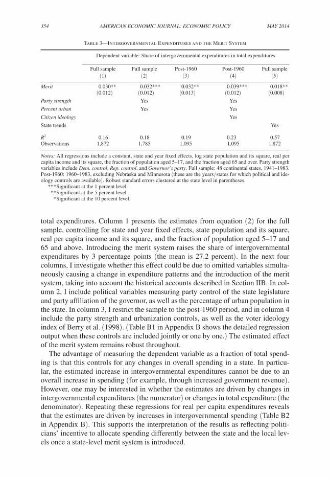
total expenditures. Column 1 presents the estimates from equation (2) for the full sample, controlling for state and year fixed effects, state population and its square, real per capita income and its square, and the fraction of population aged 5–17 and 65 and above. Introducing the merit system raises the share of intergovernmental expenditures by 3 percentage points (the mean is 27.2 percent). In the next four columns, I investigate whether this effect could be due to omitted variables simulta-neously causing a change in expenditure patterns and the introduction of the merit system, taking into account the historical accounts described in Section IIB. In col-umn 2, I include political variables measuring party control of the state legislature and party affiliation of the governor, as well as the percentage of urban population in the state. In column 3, I restrict the sample to the post-1960 period, and in column 4 include the party strength and urbanization controls, as well as the voter ideology index of Berry et al. (1998). (Table B1 in Appendix B shows the detailed regression output when these controls are included jointly or one by one.) The estimated effect of the merit system remains robust throughout.
The advantage of measuring the dependent variable as a fraction of total spend-ing is that this controls for any changes in overall spending in a state. In particu-lar, the estimated increase in intergovernmental expenditures cannot be due to an overall increase in spending (for example, through increased government revenue). However, one may be interested in whether the estimates are driven by changes in intergovernmental expenditures (the numerator) or changes in total expenditure (the denominator). Repeating these regressions for real per capita expenditures reveals that the estimates are driven by increases in intergovernmental spending (Table B2 in Appendix B). This supports the interpretation of the results as reflecting politi-cians’ incentive to allocate spending differently between the state and the local lev-els once a state-level merit system is introduced.
Table 3—Intergovernmental Expenditures and the Merit System
Dependent variable: Share of intergovernmental expenditures in total expenditures
Full sample Full sample Post-1960 Post-1960 Full sample(1) (2) (3) (4) (5)
merit 0.030** 0.032*** 0.032** 0.039*** 0.018**(0.012) (0.012) (0.013) (0.012) (0.008)
Party strength Yes Yes
Percent urban Yes Yes
citizen ideology Yes
State trends Yes
r2 0.16 0.18 0.19 0.23 0.57Observations 1,872 1,785 1,095 1,095 1,872
Notes: All regressions include a constant, state and year fixed effects, log state population and its square, real per capita income and its square, the fraction of population aged 5–17, and the fraction aged 65 and over. Party strength variables include Dem. control, rep. control, and Governor’s party. Full sample: 48 continental states, 1941–1983. Post-1960: 1960–1983, excluding Nebraska and Minnesota (these are the years/states for which political and ide-ology controls are available). Robust standard errors clustered at the state level in parentheses.
*** Significant at the 1 percent level. ** Significant at the 5 percent level. * Significant at the 10 percent level.

VoL. 6 No. 2 355ujhelyi: Civil ServiCe ruleS and PoliCy ChoiCeS
Column 5 of Table 3 presents a specification that deals with the potential endo-geneity of civil service reform in a more conservative way. Rather than including the specific controls above suggested by the historical accounts in Section IIB, this column includes state-specific time trends. This allows for cross-state differences in the trend of intergovernmental expenditures and, in contrast to the earlier esti-mates, does not attribute all differences in trends to the merit system. While natu-rally smaller than the previous estimates, this effect is also statistically significant: on average, the merit system causes a 1.8 percentage point increase in the share of intergovernmental expenditures relative to the state-specific trend.
As a final check on the validity of interpreting these estimates as causal, I include lags and leads of the merit system variable, as in equation (3). The coefficient esti-mates from this regression are graphed in Figure 1 and reported in Table B3 in Appendix B. The estimated “effect” of a merit system on the share of intergovern-mental expenditures is virtually zero in the four years preceding the introduction of the system. In the first year when expenditures occur under a merit system, the share of intergovernmental spending shifts up and stays at this higher level for the next four years. These patterns are consistent with a causal interpretation: the merit system led to an increase in the share of intergovernmental spending, and the new structure of spending seems to have stabilized for the following four–five years.
It is, of course, possible that the increase in intergovernmental spending rep-resented more than the reallocation of short-term state budgets. The incentives described in the simple model above may have led politicians to transfer entire areas of decision making to lower level governments in response to civil service reform. Thus, the estimated effect of the merit system could include both policy changes and more far-reaching institutional changes.
0.08
0.06
0.04
0.02
0
–0.02
–0.04
–0.06
–0.08
–5 –4 –3 –2 –1 0 1 2 3 4 5
Figure 1. Event Study
Notes: The figure plots coefficient estimates from regressing the fraction of intergovernmental expenditures on five leads and lags of merit (equation (3)). On the horizontal axis, negative (posi-tive) numbers denote the number of years before (after) adoption. The dotted line represents the 95 percent confidence interval. Controls include party strength, citizen ideology, percent urban, and all controls listed in the notes to Table 3. The estimation sample is post-1960, using a balanced set of states to estimate all lags and leads.

356 AmErIcAN EcoNomIc JoUrNAL: EcoNomIc PoLIcy mAy 2014
B. Employment and Payrolls
The previous section established the effect of the merit system on intergovern-mental transfers. In what follows, I ask whether interpreting the increase in transfers as politicians’ rational response to constraints created by the merit system, as in the simple model of Section III, is warranted.
As described in Section IIB, some authors have interpreted the introduction of the merit system as reflecting the strategic incentives of incumbent politicians to create entrenched bureaucracies. This would create an incentive for politicians to hire more loyal employees and perhaps increase their wages. Creating part-time positions would be especially attractive since they allow the employment of more supporters for a given budget. By contrast, if the introduction of the merit sys-tem is driven by voter demands for a more efficient bureaucracy, we would expect reform to be associated with a reduction in employment, especially among part-time workers.26
Table 4 presents estimates from equation (2) for various employment outcomes. For each outcome, I first present a regression on the full sample controlling for state and year fixed effects, state population and its square, real per capita income and its square, and the fraction of population aged 5–17 and 65 and above. I then add the party strength and urban population measures to control for these potential deter-minants of civil service reform. Next, I restrict the sample to the post-1960 period for which the citizen ideology measure is also available, and finally include all these controls.
Panel A does not support the view that introduction of the merit system led to increased employment. The merit variable is associated with a 3.5–5.4 percent reduction in employment. Panels B and C show that this is driven by part-time employees: civil service reform led to a particularly large decline of 12–16 percent in this category. Full-time employment may also have decreased but this is never statistically significant.
These findings reinforce the view that the introduction of the merit system was not just a symbolic act, but in fact contributed to streamlining state bureaucracies, which were thought to be bloated with patronage employees. There is no indication that incumbent politicians were able to use the system to put more of their loyal employees on public payrolls.27 To the extent that part-time employment is par-ticularly prone to patronage, the especially large reduction in part-time employees also supports this interpretation.28 Finally, if the merit system was used to protect entrenched bureaucrats, it might allow them to acquire higher salaries, especially given the reduction in the number of employees found above. We do not find evi-dence of this in the data. In panels D and E, introducing the merit system has an
26 While the merit system put an end to political firings, employees could still be dismissed for nonperformance. The tenure system, including the procedures for dismissal and appeals, was usually developed by the civil service commissions following the adoption of the merit system.
27 These results also offer little support for the view that an increasing labor force raised the transaction costs of patronage and caused politicians to abandon the system. If anything, merit adoption is associated with lower employment.
28 Part-time employees (who can be temporary or permanent) allow the politician to place more of his support-ers on the public payroll for a given wage bill. See Enikolopov (2012) for a different perspective.

VoL. 6 No. 2 357ujhelyi: Civil ServiCe ruleS and PoliCy ChoiCeS
Table 4—State Employees and the Merit System
Full sample Full sample Post-1960 Post-1960(1) (2) (3) (4)
Panel A. Dependent variable: log total employmentmerit −0.036 −0.054 −0.035 −0.052**
(0.035) (0.033) (0.026) (0.025)Party strength Yes YesPercent urban Yes Yescitizen ideology Yes
r2 0.96 0.96 0.95 0.95
Observations 1,680 1,601 1,095 1,095
Panel B. Dependent variable: log full-time employmentmerit −0.004 −0.020 −0.024 −0.044
(0.035) (0.035) (0.029) (0.027)Party strength Yes YesPercent urban Yes Yescitizen ideology Yes
r2 0.95 0.95 0.94 0.94
Observations 1,680 1,601 1,095 1,095
Panel c. Dependent variable: log part-time employmentmerit −0.141** −0.162** −0.115* −0.119*
(0.068) (0.070) (0.063) (0.063)Party strength Yes YesPercent urban Yes Yescitizen ideology Yes
r2 0.75 0.79 0.82 0.82
Observations 1,680 1,601 1,095 1,095
Panel D. Dependent variable: log total monthly payrollmerit −0.011 −0.026 −0.017 −0.034
(0.037) (0.036) (0.036) (0.033)Party strength Yes YesPercent urban Yes Yescitizen ideology Yes
r2 0.98 0.98 0.95 0.95
Observations 1,680 1,601 1,095 1,095
Panel E. Dependent variable: log average full-time equivalent wagemerit −0.003 0.002 0.016 0.017
(0.011) (0.012) (0.015) (0.016)Party strength Yes YesPercent urban Yes Yescitizen ideology Yes
r2 0.94 0.94 0.80 0.80
Observations 1,440 1,371 1,095 1,095
Notes: All regressions include a constant, state and year fixed effects, log state population and its square, real per capita income and its square, the fraction of population aged 5–17, and the fraction aged 65 and over. Party strength variables include Dem. control, rep. control, and Governor’s party. Full sample: 48 continental states, 1945–1983 in panels A–D, 1951–1983 in panel E; post-1960: 1960–1983, excluding Nebraska and Minnesota (these are the years/states for which political and ideology controls are available). Robust standard errors clustered at the state level in parentheses.
*** Significant at the 1 percent level. ** Significant at the 5 percent level. * Significant at the 10 percent level.

358 AmErIcAN EcoNomIc JoUrNAL: EcoNomIc PoLIcy mAy 2014
insignificant negative effect on monthly payroll expenditures and an insignificant effect on average full-time equivalent wages.
C. Intergovernmental Expenditures on Welfare and roads
The model in Section III considers public good spending that delivers private benefits to the politician (perhaps through patronage opportunities or through elec-toral support). Thus, we should expect to observe an increase in the share of inter-governmental spending within such politically salient categories.
Table 5 asks whether politicians’ incentives to shift expenditures to bureaucrats not affected by the merit system can be observed for welfare expenditures (panel A) and spending on roads (panel B). Both of these categories are commonly viewed as politically important and prone to political targeting (see, e.g., Dye 1984 and Knight 2002). At the same time, a large degree of bureaucratic discretion is involved in deciding where and how the money is actually spent. For example, welfare recipi-ents have to go through an approval process, and investment projects go through government procurement.
In both panels, the dependent variable is the ratio of intergovernmental to total expenditures in the given category. I find that these shares increase significantly once the merit system is introduced. The increase in intergovernmental welfare
Table 5—Intergovernmental Expenditures on Welfare and Roads
Full sample Full sample Post-1960 Post-1960(1) (2) (3) (4)
Panel A. Dependent variable: Share of IG expenditures in welfare expendituresmerit 0.085* 0.138*** 0.120*** 0.160***
(0.048) (0.039) (0.040) (0.046)Party strength Yes YesPercent urban Yes Yescitizen ideology Yes
r2 0.38 0.40 0.38 0.42Observations 1,632 1,555 1,095 1,095
Panel B. Dependent variable: Share of IG expenditures in spending on roadsmerit 0.022* 0.022* 0.018** 0.015*
(0.011) (0.012) (0.008) (0.008)Party strength Yes YesPercent urban Yes Yescitizen ideology Yes
r2 0.32 0.33 0.22 0.22Observations 1,872 1,785 1,095 1,095
Notes: All regressions include a constant, state and year fixed effects, state population and its square, real per capita income and its square, the fraction of population aged 5–17, and the fraction aged 65 and over. Party strength variables include Dem. control, rep. control, and Governor’s party. Full sample: 48 continental states, 1950–1983 in panel A, 1941–1983 in panel B. Post-1960: 1960–1983, excluding Nebraska and Minnesota (these are the years/states for which political and ideology controls are available). Robust standard errors clustered at the state level in parentheses
*** Significant at the 1 percent level. ** Significant at the 5 percent level. * Significant at the 10 percent level.
VoL. 6 No. 2 359ujhelyi: Civil ServiCe ruleS and PoliCy ChoiCeS
expenditures is especially sizeable: 9–16 percentage points relative to a mean of 22 percent. The estimates are similar in the full and the post-1960 sample and are increased by the inclusion of urbanization, party strength and citizen ideology. The estimated increase in intergovernmental spending on roads is 1.5–2.2 percentage points relative to a mean of 17.8 percent. These results are also robust to the inclu-sion of controls.
As a comparison, Table B4 in Appendix B presents similar regressions for an exhaustive list of expenditure categories. With the possible exception of education spending, which yields a statistically significant positive coefficient for the more recent sample, the effect of merit on these categories is always small and insignifi-cant, and it is often negative. For expenditures on public safety, hospitals, financial administration, or natural resources, we do not observe the kind of reallocation that we found for the more politicized categories of welfare and highway spending.29
These findings are consistent with the idea that politicians direct politically rel-evant spending through channels where they have more control over policy imple-mentation. The particularly large decline in the share of direct expenditures in welfare spending is especially suggestive. Bureaucratic discretion can play a large role in the allocation of cash transfers, and therefore the merit system has a large impact on politicians’ ability to influence where the money ends up.
D. Further Evidence from Detailed regulations
While all state-level merit systems formally ended patronage and moved the bureaucracy towards the Weberian ideal, there is variation in the operation of per-sonnel systems across states. This variation can be used to assess the validity of the findings and interpretations presented above.
One concern with the findings reported above is whether state governments might explicitly encourage the establishment of local merit systems following civil ser-vice reform at the state level. If that was the case, it could be that intergovernmen-tal transfers reflect state assistance for the development of civil service procedures (e.g., testing procedures) at the local levels.
To the extent possible, I checked whether the state-level merit system contained any provisions for the merit systems of lower level governments such as cities or counties. I found three types of relevant provisions. (i) A statute might state that local governments subject to federal grant-in-aid requirements should have a merit system. Since this provision restates a requirement imposed earlier by the federal government (mostly in 1939–1940, as described above) it does not represent a change in regulations. (ii) A statute might state that the state personnel board can enter into agreements with lower level governments to “furnish services and facili-ties in the administration of its personnel program” (e.g., 1967 Florida Statutes, Chapter 110, section 110.071). These agreements are not mandatory; moreover, the provisions typically specify that the local government should reimburse the state personnel board for its expenses. Therefore, these agreements would not be reflected
29 I explore education spending further in Section VE below.

360 AmErIcAN EcoNomIc JoUrNAL: EcoNomIc PoLIcy mAy 2014
in intergovernmental expenditures from the state to the local government unit. If any-thing, payments would flow in the opposite direction. (iii) I found a single instance where a state-level statute required a local government unit to establish a new merit system: the 1952 Constitution of Louisiana establishing the state-level merit system also required one city, New Orleans, to establish such a system (Article XIV). Thus, the state-to-local transfers in Louisiana during this period could conceivably reflect direct assistance by the state government to the city of New Orleans in establishing its merit system. I checked that excluding Louisiana from the regressions leaves my results intact.
Another useful characteristic of state merit systems is whether the personnel executive is independent of the governor. Despite similar merit system provisions, the de facto separation between bureaucrats and politicians may be weaker when the personnel executive is appointed by the governor. If the interpretation that the shift from direct to intergovernmental spending reflects politicians’ rational response to a more independent bureaucracy is correct, these patterns should also appear when comparing merit systems with and without an independent personnel executive. A personnel executive who is independent of the governor reinforces the separation between the political executive and the bureaucrats implementing his policies. In this case, the incumbent politician should have added incentive to shift spending away from state-level bureaucrats and towards lower level governments. To measure this, the variable IPE takes the value of zero if the personnel executive is appointed by the governor and 1 in all other cases (appointed by civil service commission, personnel board, or department head).
In Table 6, I estimate the effect of IPE on the share of all intergovernmental expenditures in total spending, as well as the shares within welfare expenditures and spending on roads. Since the IPE variable also takes the value of zero in the absence of a merit system, the coefficient estimates listed in the second row measure the impact of an independent executive relative to a merit system where the execu-tive is not independent from the governor. The coefficients on merit in the first row measure the impact of a merit system with no independent executive relative to no merit system, and I also report an F-test for the hypothesis that the sum of these two coefficients is zero (i.e., testing the impact of a merit system with an independent executive relative to a situation with no merit system). Since a personnel executive independent from the governor may increase the independence of the bureaucracy as a whole, we expect the effect of this variable to reinforce the effects of a merit system.30
The findings in Table 6 confirm this interpretation. In column 1, introducing a merit system with no independent executive increases the share of intergovernmen-tal spending by 2.8 percentage points, and making the executive independent adds a further 1.1 percentage points. I find similar results in columns 2 (welfare) and 3 (highways): in both cases, the merit and IPE coefficients have the same sign and are generally statistically significant. Thus, an independent personnel executive further reinforces the effect of the merit system on the division of state spending
30 Because information on the personnel executive is only available starting in 1965, I lose the majority of the policy changes used to identify the effect of merit in the previous regressions.

VoL. 6 No. 2 361ujhelyi: Civil ServiCe ruleS and PoliCy ChoiCeS
between direct and intergovernmental expenditures. As expected, politicians adjust their behavior not simply in response to the introduction of the merit system, but also in response to the marginal incentives created by specific features of that system. The closer the system is to the Weberian ideal of a complete separation between politicians and bureaucrats, the more politicians spend outside the bureaucracy that it regulates.
E. Alternative Explanations
This section considers threats to identification and alternative explanations not ruled out by the specifications above.
Federal IG Transfers.—One might be concerned about the role of earmarked intergovernmental transfers from the federal government. The federal government spends a substantial amount at the local level, and it may prefer spending money through bureaucrats subject to a merit system. State bureaucracies under a merit sys-tem may be asked to administer federal transfers to local governments. Civil service reform could therefore lead to increased federal-to-local transfers administered by the state, which may show up in the data as increased state-to-local transfers, even if all that has changed is the channel through which the money flows.
A priori, this is unlikely to drive the results, since most agencies administering federal grants were required to adopt a merit system in 1939–1940, even if the state had no comprehensive merit system (see Section II). Thus, the merit variable cap-tures reform among precisely those bureaucrats who are unlikely to be administer-ing federal funds. Table B5 in Appendix B confirms that federal grants going to the state government are not related to the presence of a merit system. Regressing the former on the latter yields small and insignificant estimates.
Table 6—Independent Personnel Executive
Dependent variable: Share of IG exp. in total Share of IG exp. in welfare Share of IG exp. in roads(1) (2) (3)
merit 0.028** 0.104** 0.007(0.011) (0.048) (0.010)
IPE 0.011* 0.049* 0.020**(0.006) (0.028) (0.009)
Party strength Yes Yes YesPercent urban Yes Yes Yescitizen ideology Yes Yes Yes
r2 0.25 0.35 0.20
Observations 805 805 805
F-test: merit + IPE = 0 13.602 10.474 9.127
p-value 0.001 0.002 0.004
Notes: All regressions include a constant, state and year fixed effects, state population and its square, real per capita income and its square, the fraction of population aged 5–17, and the fraction aged 65 and over. Party strength vari-ables include Dem. control, rep. control, and Governor’s party. Sample: 46 continental states (excluding Nebraska and Minnesota), 1965–1983. Robust standard errors clustered at the state level in parentheses.
*** Significant at the 1 percent level. ** Significant at the 5 percent level. * Significant at the 10 percent level.
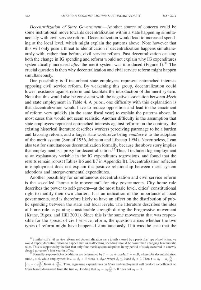
362 AmErIcAN EcoNomIc JoUrNAL: EcoNomIc PoLIcy mAy 2014
Decentralization of State Government.—Another source of concern could be some institutional move towards decentralization within a state happening simulta-neously with civil service reform. Decentralization would lead to increased spend-ing at the local level, which might explain the patterns above. Note however that this will only pose a threat to identification if decentralization happens simultane-ously with, rather than before, civil service reform. Past decentralization causing both the change in IG spending and reform would not explain why IG expenditures systematically increased after the merit system was introduced (Figure 1).31 The crucial question is then why decentralization and civil service reform might happen simultaneously.
One possibility is if incumbent state employees represent entrenched interests opposing civil service reform. By weakening this group, decentralization could lower resistance against reform and facilitate the introduction of the merit system. Note that this would also be consistent with the negative association between merit and state employment in Table 4. A priori, one difficulty with this explanation is that decentralization would have to reduce opposition and lead to the enactment of reform very quickly (in the same fiscal year) to explain the patterns above. In most cases this would not seem realistic. Another difficulty is the assumption that state employees represent entrenched interests against reform: on the contrary, the existing historical literature describes workers perceiving patronage to be a burden and favoring reform, and a larger state workforce being conducive to the adoption of the merit system (Sorauf 1956, Johnson and Libecap 1994). Nevertheless, I can also test for simultaneous decentralization formally, because the above story implies that employment is a proxy for decentralization.32 Thus, I included log employment as an explanatory variable in the IG expenditures regressions, and found that the results remain robust (Tables B6 and B7 in Appendix B). Decentralization reflected in employment does not explain the positive relationship between merit system adoptions and intergovernmental expenditures.
Another possibility for simultaneous decentralization and civil service reform is the so-called “home rule movement” for city governments. City home rule describes the power to self-govern—at the most basic level, cities’ constitutional right to modify their own charters. It is an indication of the importance of local governments, and is therefore likely to have an effect on the distribution of pub-lic spending between the state and local levels. The literature describes the idea of home rule as gaining considerable strength during the Progressive movement (Krane, Rigos, and Hill 2001). Since this is the same movement that was respon-sible for the spread of civil service reform, the question arises whether the two types of reform might have happened simultaneously. If it was the case that the
31 Similarly, if civil service reform and decentralization were jointly caused by a particular type of politician, we would expect decentralization to happen first as reallocating spending should be easier than changing bureaucratic rules. This is supported by the fact that only four merit system adoptions in my period of study occurred in a newly elected governor’s first year in office.
32 Formally, suppose IG expenditures are determined by y = α 0 + α 1 merit + α 2 D, where D is decentralization and α 2 > 0, while employment is L = β 0 + β 1 merit + β 2 D, where β 1 ≤ 0 and β 2 < 0. Then y = α 0 − α 2
β 0 _ β 2 +
( α 1 − α 2 β 1
_ β 2 ) merit + α 2
_ β 2 L. Thus, regressing expenditures on merit and employment will produce a coefficient on
merit biased downward from the true α 1 . Finding that α 1 − α 2 β 1
_ β 2 > 0 rules out α 1 = 0.

VoL. 6 No. 2 363ujhelyi: Civil ServiCe ruleS and PoliCy ChoiCeS
states enacted home rule laws in the same periods as they introduced the merit sys-tem, this could potentially explain the increase in state-to-local transfers observed in the data.
To check this, I use the dates of adoption of home rule provisions collected by Krane, Rigos, and Hill (2001). A state is categorized as “home rule state” if it allows at least the most basic form of autonomy (“structural home rule”), and the date listed corresponds to the enactment of such legislation (typically a constitutional amend-ment). Comparing this data to the dates of merit system adoption does not indicate a connection between the timing of home rule provisions and civil service reform. Twenty-two of the states that introduced the merit system during my period of study also adopted home rule provisions at some point in time. However, only two of these did so in the ten years preceding the introduction of the merit system (Montana four years before, Missouri in the same year). Thus, controlling for whether the state has a home rule provision on the books in a given year does not affect my results (Tables B6 and B7 in Appendix B). In fact, eight states introduced home rule provisions in the ten years following civil service reform. Based on the model in Section III, such decentralization could be a response to civil service reform.
Immigrants.—Several descriptions of local US politics in the early twentieth century highlight the role of patronage networks based on ethnicity among recent immigrants (see, e.g., Clark 1975 on patronage among the Irish in Boston). It is also conceivable that a state facing a sudden influx of immigrants sees more demand for local support in the form of intergovernmental transfers. Thus, the fraction of immigrants could, in principle, be a relevant omitted variable. Whether this would go against or reinforce the findings above is theoretically unclear: more immigration could increase demand for patronage and make civil service reform less likely. Alternatively, civil service reform could be a way to break traditional patronage networks and allow new immigrants a chance at obtaining public jobs, which would make reform more likely (Ruhil and Camões 2003). In Tables B6 and B7 in Appendix B, I also control for the fraction of the state population that is foreign-born, and find that the estimates above remain robust both in sign and in magnitude.
Education Spending.—A question arises regarding the treatment of education spending. On the one hand, school districts are autonomous government units with their own politics that, in many respects, resemble that of other local governments (see, e.g., Moe 2006). Therefore, once a state-level merit system is adopted, state politicians may have similar incentives to increase transfers to school districts as they have for other local governments. On the other hand, education may be viewed as a large and heterogenous area of spending with its own reorganization reforms throughout the twentieth century. The above findings might be less convincing if they were driven exclusively by education spending. I have checked that this is not the case by subtracting all education spending from the corresponding catego-ries and rerunning the regressions (see Table B8 in Appendix B). As expected, the results are somewhat weaker but the coefficients always have the right sign and are generally statistically significant.

364 AmErIcAN EcoNomIc JoUrNAL: EcoNomIc PoLIcy mAy 2014
F. Some city-Level Evidence
The model in Section III implies that some local governments should see an increase in intergovernmental transfers from the state once a state-level merit sys-tem is introduced. If such reallocation of spending is indeed driven by politicians’ self-interest, it is natural to expect localities aligned with the governor to receive more transfers.
Testing this prediction creates considerable data challenges. Ideally, it would require information on both local politics and government finances for my period of study for a sample of different types of local governments within each state, to capture all the possible recipients of state intergovernmental transfers. This ideal data is not available. Instead, I present some suggestive evidence focusing on US cities using Ferreira and Gyourko’s (2009) dataset on mayors’ party affiliation. I merge this with my state-level data to create a measure of party alignment between mayors and state governors for an unbalanced panel of 147 cities in 42 states.33 In this sample, I estimate
y cst = α 1 meri t st + α 2 Alignedmayo r cst + α 3 meri t st × Alignedmayo r cst
+ β 1 X st + β 2 X cst + γ c + δ t + ε cst ,
where y cst is the log per capita IG revenue in city c, state s, time t, Alignedmayor equals 1 if the mayor is from the same party as the state governor, X st are the same controls used in the state-level regressions above, X cst are the available time varying city-level controls (log city population and its square, and party of the mayor), and γ c and δ t are city and year fixed effects, respectively.
The results from this regression are in Table 7. In column 1, estimating the regres-sion without the interaction term indicates that, on average, a city receives 5 percent more transfers from the state when its mayor is aligned with the governor. Column 2 shows that this effect is driven by city-years when a state-level merit system is in place. The interaction between merit and Alignedmayors indicates that the differ-ence in transfers to aligned versus nonaligned mayors is significantly larger under a merit system than without a merit system. This is consistent with state politicians’ increased incentives to transfer resources to aligned mayors under a merit system, as suggested by the above model. Columns 3–4 on the post-1960 sample confirm these patterns.34
Given the data constraints mentioned above, these findings are merely sugges-tive. Nevertheless, they do indicate that state-level bureaucratic reforms may have
33 See Appendix A for details on the data. I restrict attention to cities with a population of at least 50,000 as the political importance of small towns is likely to be limited. The Ferreira and Gyourko (2009) data only contains directly elected mayors. When available, I supplement this with information on the party affiliation of indirectly elected mayors for the largest city in each state.
34 Somewhat surprisingly, in columns 2 and 4 the baseline (no merit system) difference between aligned and nonaligned mayors is negative, although not statistically significant. One possible explanation is that intergovern-mental transfers may be an inferior tool for achieving political goals: state politicians may only rely on them if forced to do so by the merit system.

VoL. 6 No. 2 365ujhelyi: Civil ServiCe ruleS and PoliCy ChoiCeS
important ramifications for local public finances along the lines suggested by the above model.
VI. How Does Bureaucratic Reform Affect Public Investment?
The preceding sections showed that politicians respond to bureaucratic reform at the state level by relying more heavily on local governments in the administration of state expenditures. Does this reallocation of expenditures, in turn, have an effect on the level of spending?
Rauch (1995) has found that municipal reforms in the Progressive Era led to more investment on roads, sewerage, and water infrastructure at the city level. He interprets these findings in a framework where bureaucrats can directly influence politicians’ behavior by providing them with selective information. The increase in job security afforded by the merit system extends bureaucrats’ time horizon, leads them to favor long-run projects, and they convince the politician to spend more in these areas. While this story may be an accurate description of reform in lower level governments, an important difference between local governments and state govern-ments is the ability to transfer resources to lower level governments in the same jurisdiction. Above, I have shown that state governments responded to civil ser-vice reform in their bureaucracies by making such transfers. This suggests that the impact on total infrastructure investments (the sum of direct and intergovernmental spending) may also differ between these levels of government.
Table 8 investigates the effect of the merit system on investment projects by state governments. In panel A, the dependent variable is the share of capital outlays on roads in total state expenditures, and I find that introducing the merit system reduces state government spending in this category. The estimated coefficient is between
Table 7—City Revenue from State IG Transfers, and the Merit System
Dependent variable: City IG revenue from the state
Full sample Full sample Post-1960 Post-1960(1) (2) (3) (4)
merit 0.208 0.094 0.282 0.151(0.282) (0.265) (0.379) (0.383)
Alignedmayor 0.050 −0.093 0.038 −0.105(0.030) (0.075) (0.030) (0.080)
merit × 0.168* 0.164* Alignedmayor (0.092) (0.096)r2 0.51 0.51 0.46 0.46Observations 2,916 2,916 2,343 2,343
Notes: The dependent variable is log per capita city revenue from state IG transfers. All regres-sions include a constant, city and year fixed effects, log city population and its square, party of the mayor, log state population and its square, real state per capita income and its square, the fraction of population aged 5–17, the fraction aged 65 and over, and state-level party strength variables. Columns 3 and 4 also include citizen ideology. The sample includes 147 cities and 42 states, 1951–1983 (full sample), 1960–1983 (post-1960). Robust standard errors clustered at the state level in parentheses.
*** Significant at the 1 percent level. ** Significant at the 5 percent level. * Significant at the 10 percent level.
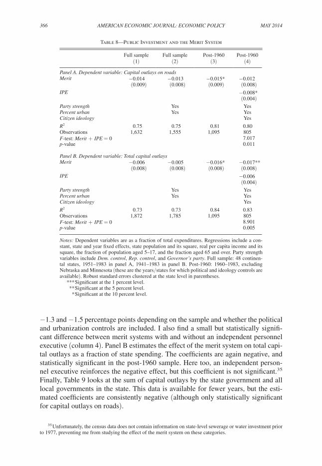
366 AmErIcAN EcoNomIc JoUrNAL: EcoNomIc PoLIcy mAy 2014
−1.3 and −1.5 percentage points depending on the sample and whether the political and urbanization controls are included. I also find a small but statistically signifi-cant difference between merit systems with and without an independent personnel executive (column 4). Panel B estimates the effect of the merit system on total capi-tal outlays as a fraction of state spending. The coefficients are again negative, and statistically significant in the post-1960 sample. Here too, an independent person-nel executive reinforces the negative effect, but this coefficient is not significant.35 Finally, Table 9 looks at the sum of capital outlays by the state government and all local governments in the state. This data is available for fewer years, but the esti-mated coefficients are consistently negative (although only statistically significant for capital outlays on roads).
35 Unfortunately, the census data does not contain information on state-level sewerage or water investment prior to 1977, preventing me from studying the effect of the merit system on these categories.
Table 8—Public Investment and the Merit System
Full sample Full sample Post-1960 Post-1960(1) (2) (3) (4)
Panel A. Dependent variable: capital outlays on roadsmerit −0.014 −0.013 −0.015* −0.012
(0.009) (0.008) (0.009) (0.008)IPE −0.008*
(0.004)Party strength Yes YesPercent urban Yes Yescitizen ideology Yes
r2 0.75 0.75 0.81 0.80Observations 1,632 1,555 1,095 805F-test: merit + IPE = 0 7.017p-value 0.011
Panel B. Dependent variable: Total capital outlaysmerit −0.006 −0.005 −0.016* −0.017**
(0.008) (0.008) (0.008) (0.008)IPE −0.006
(0.004)Party strength Yes YesPercent urban Yes Yescitizen ideology Yes
r2 0.73 0.73 0.84 0.83Observations 1,872 1,785 1,095 805F-test: merit + IPE = 0 8.901p-value 0.005
Notes: Dependent variables are as a fraction of total expenditures. Regressions include a con-stant, state and year fixed effects, state population and its square, real per capita income and its square, the fraction of population aged 5–17, and the fraction aged 65 and over. Party strength variables include Dem. control, rep. control, and Governor’s party. Full sample: 48 continen-tal states, 1951–1983 in panel A, 1941–1983 in panel B. Post-1960: 1960–1983, excluding Nebraska and Minnesota (these are the years/states for which political and ideology controls are available). Robust standard errors clustered at the state level in parentheses.
*** Significant at the 1 percent level. ** Significant at the 5 percent level. * Significant at the 10 percent level.
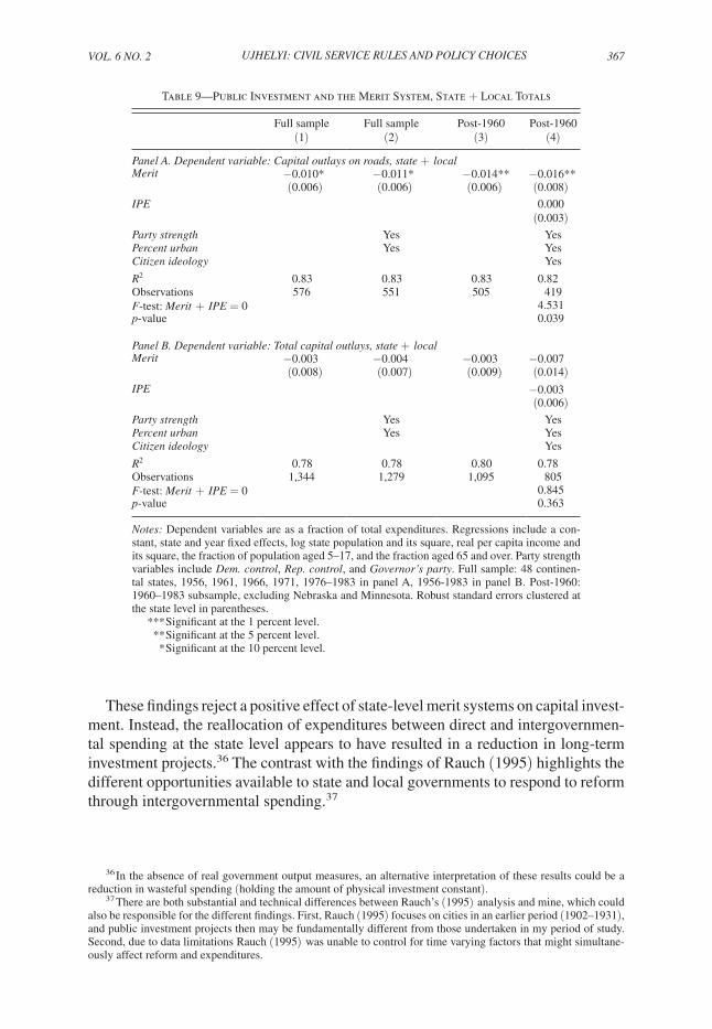
VoL. 6 No. 2 367ujhelyi: Civil ServiCe ruleS and PoliCy ChoiCeS
These findings reject a positive effect of state-level merit systems on capital invest-ment. Instead, the reallocation of expenditures between direct and intergovernmen-tal spending at the state level appears to have resulted in a reduction in long-term investment projects.36 The contrast with the findings of Rauch (1995) highlights the different opportunities available to state and local governments to respond to reform through intergovernmental spending.37
36 In the absence of real government output measures, an alternative interpretation of these results could be a reduction in wasteful spending (holding the amount of physical investment constant).
37 There are both substantial and technical differences between Rauch’s (1995) analysis and mine, which could also be responsible for the different findings. First, Rauch (1995) focuses on cities in an earlier period (1902–1931), and public investment projects then may be fundamentally different from those undertaken in my period of study. Second, due to data limitations Rauch (1995) was unable to control for time varying factors that might simultane-ously affect reform and expenditures.
Table 9—Public Investment and the Merit System, State + Local Totals
Full sample Full sample Post-1960 Post-1960(1) (2) (3) (4)
Panel A. Dependent variable: capital outlays on roads, state + localmerit −0.010* −0.011* −0.014** −0.016**
(0.006) (0.006) (0.006) (0.008)IPE 0.000
(0.003)Party strength Yes YesPercent urban Yes Yescitizen ideology Yes
r2 0.83 0.83 0.83 0.82Observations 576 551 505 419F-test: merit + IPE = 0 4.531p-value 0.039
Panel B. Dependent variable: Total capital outlays, state + localmerit −0.003 −0.004 −0.003 −0.007
(0.008) (0.007) (0.009) (0.014)IPE −0.003
(0.006)Party strength Yes YesPercent urban Yes Yescitizen ideology Yes
r2 0.78 0.78 0.80 0.78Observations 1,344 1,279 1,095 805F-test: merit + IPE = 0 0.845p-value 0.363
Notes: Dependent variables are as a fraction of total expenditures. Regressions include a con-stant, state and year fixed effects, log state population and its square, real per capita income and its square, the fraction of population aged 5–17, and the fraction aged 65 and over. Party strength variables include Dem. control, rep. control, and Governor’s party. Full sample: 48 continen-tal states, 1956, 1961, 1966, 1971, 1976–1983 in panel A, 1956-1983 in panel B. Post-1960: 1960–1983 subsample, excluding Nebraska and Minnesota. Robust standard errors clustered at the state level in parentheses.
*** Significant at the 1 percent level. ** Significant at the 5 percent level. * Significant at the 10 percent level.
368 AmErIcAN EcoNomIc JoUrNAL: EcoNomIc PoLIcy mAy 2014
VII. Conclusion
To understand the costs and benefits of bureaucratic reform, one needs to look beyond the immediate impact of reform on bureaucrats’ behavior. Rules governing the operation of bureaucracies constrain politicians and may, therefore, affect the policies adopted. For example, while few would dispute that it is desirable to have qualified bureaucrats in charge of implementing any given policy, the welfare evalu-ation of merit-based recruitment requires understanding how reforms may change the policies that bureaucrats will be required to implement.
This paper has used new data on the timing of civil service reforms in US states to study the effect of bureaucratic rules on policymaking. My results show that state governments respond to civil service regulations by increasing their reliance on local governments in administering state spending. Such reallocation is also observed for politically sensitive categories like welfare and roads. This is consistent with politi-cians rationally substituting away from expenditures where they are constrained in their ability to pursue their self-interest. In turn, I find evidence that the reallocation of expenditures leads to lower total spending on long-term capital projects.
Did the merit system raise social welfare? Measuring the quality of government performance is notoriously hard, and I am not aware of any data that would allow addressing this question directly in the present context. Thus, the above results only warrant normative statements under certain assumptions. First, in the context of the model presented in Section III, the increase in intergovernmental transfers following reform has negative implications for social welfare as long as state-level bureaucrats were at least as productive as local bureaucrats before reform (α ≥ β). Second, in the context of previous studies that have argued that government investment in infrastructure leads to economic growth, the findings in Section VI of a reduction in investment also have negative welfare implications. However, even if reform had an undesirable effect on politicians’ choices, it is possible that this was more than offset by direct improvements in the functioning of the bureaucracy. My results provide one ingredient to the welfare analysis of civil service regulations by emphasizing that reforms affect the policy choices of elected politicians.
Although my quantitative findings are specific to the institutions and period being studied, the results have broad policy implications for current reform proposals, especially in the context of a federal system. For example, the introduction men-tioned several US states that have recently made steps towards weakening the civil service protections of state employees. While critics have worried about a return of patronage practices, my paper suggests a complementary consideration. If these state-level reforms are not accompanied by similar changes at the local level, pol-iticians may have an incentive to reduce the fraction of spending going to local governments.
Clearly, politicians may react to civil service rules in other dimensions as well. For example, Iyer and Mani (2012) argue that while constrained by civil service rules, politicians in India are able to control bureaucrats by threatening them with reassignment to less desirable positions. Influence is also possible by redesign-ing the administrative procedures of government agencies (McCubbins, Noll, and Weingast 1987). Studying whether civil service reform affects the reassignment of

VoL. 6 No. 2 369ujhelyi: Civil ServiCe ruleS and PoliCy ChoiCeS
bureaucrats, administrative procedures, or other aspects of politicians’ behavior is an interesting topic for future research.
Appendix A: Data Sources and Definitions
A. merit System
For all states, the sources include The Book of the States, Lexington, KY: The Council of State Governments (various issues) as well as Civil Service Assembly of the United States and Canada: civil Service Agencies in the United States, Pamphlets Nos. 11 (1937), 16 (1940), and 17 (1943). Additional state-specific sources are listed below.
Arizona: Kellough and Nigro (2006, ch. 8). Arizona State Personnel Commission (1970): Annual report 1968-69, Phoenix, AZ: Arizona State Personnel Commission.
Arkansas: Blair, D. D., and J. Barth (2005): Arkansas politics and govern-ment, Lincoln, NE: University of Nebraska Press; Uniform Classification and Compensation Act (Act 199 of 1969); Holley, D. (1986): “Carl E. Bailey, the Merit System, and Arkansas Politics, 1936-1939,” Arkansas Historical Quarterly 45, 291–320.
colorado: Buchanan, D. V. (1932): The merit system in colorado, MA thesis, University of Colorado.
Delaware: Boyer, W. W. (2000): Governing Delaware: Policy Problems in the First State, Cranbury, NJ: Associated University Presses. Title 29, Chapter 59, DE Code.
Florida: Kellough and Nigro (2006, ch. 7). Florida Statutes 1967, Chapter 110 available at http://archive.org/details/FloridaStatutes1967Volume1.
Georgia: Constitution of 1945, Article XIV.Idaho: Rules and Regulations of the Idaho Personnel Commission: Adopted
January 5, 1967.Iowa: “Senate votes in merit system,” Ames Daily Tribune, April 14, 1967, 1. The
rules of the merit System of Iowa, 1971, Des Moines, IA: Iowa Merit Employment Department.
Kentucky: Schten, E. V. (1960): “Forward in Kentucky,” National civic review, Volume 49, 6, 302–307.
Louisiana: Owen, K. (1952): “Amendments to the Louisiana Constitution,” Louisiana Law review 13, 219–229.
michigan: Dunbar, W. F., and G. S. May (1995): michigan: A History of the Wolverine State, Grand Rapids, MI: Wm. B. Eerdmans Publishing.
mississippi: General laws of 1976, Chapter 377.missouri: Faust, M. L. (1946): “Reorganization in Missouri,” National municipal
review 35(8), 402–407.montana: Montana Department of Administration (1974): Statewide Classification
and Pay Plans, Report to Governor Thomas L. Judge, Helena, MT: State of Montana Department of Administration. Montana Legislative Audit Division (1997): Personnel Classification, Performance Survey Report to the Legislature, Helena, MT: State of Montana Legislative Audit Division.

370 AmErIcAN EcoNomIc JoUrNAL: EcoNomIc PoLIcy mAy 2014
Nevada: 1953 Statutes of Nevada, Chapter 351.New Hampshire: Supreme Court of New Hampshire (1978): The State Employees’
Association of New Hampshire, Inc. V. The New Hampshire Public Employee Labor relations Board, December 29, 1978. At http://nh.findacase.com/research/wfrmDocViewer.aspx/xq/fac.19781229_0015.NH.htm/qx.
New mexico: Hain, P. L., C. Garcia, and G. K. St Clair (1994): New mexico Government, University of New Mexico Press.
North carolina: NC Office of Archives and History (2009): http://www.stateschedules.ncdcr.gov/AgencyHistory.aspx?L1=Office%20of%20State%20Personnel.
North Dakota: ND Office of Management and Budget (2010): http://www.nd.gov/hrms/about/history.html.
oklahoma: Oklahoma Office of Personnel Management (2005): http://www.ok.gov/opm/About_OPM/Our_History/index.html.
oregon: Stahl, O. G. (1956): Public Personnel Administration, fourth ed., New York, NY: Harper and Brothers.
Pennsylvania: Pennsylvania State Archives (2012) http://www.phmc.state.pa.us/bah/dam/rg/rg3ahr.htm.
South carolina: Kellough and Nigro (2006, ch. 8).South Dakota: SD Statutes and Codes, Title 3 at http://www.find-laws.com/
statutes/south-dakota.Vermont: Stahl, O. G. (1956): Public Personnel Administration, fourth ed., New
York, NY: Harper and Brothers. VT Department of Human Resources (2012): Vermont Civil Service and the Merit System at http://humanresources.vermont.gov/services/new_employee_orientation/merit_system.
Washington: Washington State Department of Personnel (1989): A History of Personnel Systems for Washington State, Olympia, WA.
West Virginia: WV Division of Personnel (2012): http://www.state.wv.us/admin/personnel/.
Wyoming: Office of the Attorney General of Wyoming (2011): Formal Opinion 2011-002, August 25, 2011.
B. Independent Personnel Executive
Source: The Book of the States, Lexington, KY: The Council of State Governments (various issues). Takes the value of zero if personnel executive appointed by the governor, one o/w (appointed by personnel board, department head, or civil service commission). Years available: from 1965.
C. other Data
consumer Price Index (cPI).—Source: US Department of Labor: Bureau of Labor Statistics, http://www.bls.gov. Consumer Price Index for All Urban Consumers, not seasonally adjusted. Yearly value obtained by averaging across months. 1982–1984 = 100.

VoL. 6 No. 2 371ujhelyi: Civil ServiCe ruleS and PoliCy ChoiCeS
Employment and Payroll Data.—Source: US Census Bureau: Public Employment Report Series Historical Data Base, state government variables. Total Employees, Total Payrolls. Years available: from 1946, with 1951 missing. Total Full-time Employees, Part-time employment = Total Employees—Total Full-time Employees, Average full-time equivalent wage = Total Payrolls/Total Full-time Equivalent employment. Years available: from 1946, with 1951 and 1958–1960 missing.
State Expenditures.—Source: US Census Bureau, State Government Finances Publication Historical Data Base, state government variables. Total Expenditure, IG Exp-To Local Govts, Direct Expenditure, Total Capital Outlays, Regular Hwy-Total Exp, Regular Hwy-Total IG, Public Welf-Total Exp, Fin Admin and General Control-Total Exp, Public Safety-Total Exp, Total Educ-Total Exp, Total Educ-IG Exp, Total Nat Res-Tot Exp. Available years: from 1942, with 1943, 1945, 1947, 1949 missing. Public Welf-Tot IG Exp. Available years: from 1951. Fin Admin and General Control-Total IG Exp. Available years: from 1953. Public Safety-Total IG Exp. Available years: from 1951, with 1960 missing. Total Hospital-Tot Exp, Total Hospital-Total IG Exp Available years: from 1956. Total Nat Res-Tot IG. Available years: 1953–1964, 1967, 1972, 1977–.
Detailed definitions (http://www.census.gov/govs/state/definitions.html).
IG expenditures: “Amounts paid to other governments for performance of specific functions or for general financial support. Includes grants, shared taxes, contingent loans and advances, and any significant and identifiable amounts or reimbursement paid to other governments for performance of general government services or activities. Excludes amounts paid to other governments for purchase of commodities, property, or utility services and for any tax levied as such on facilities of the government.”
Capital outlays: “Expenditure for contract or force account construction of build-ings, grounds, and other improvements, and purchase of equipment, land, and exist-ing structures. Includes amounts for additions, replacements, and major alterations to fixed works and structures. However, expenditure for repairs to such works and structures is classified as current operation expenditure.”
Welfare expenditures: “Support of and assistance to needy persons contingent upon their need. Excludes pensions to former employees and other benefits not contingent on need. Expenditures under this heading include: Cash assistance paid directly to needy persons under the categorical programs (Old Age Assistance, Temporary Assistance for Needy Families (TANF) and under any other welfare programs; Vendor payments made directly to private purveyors for medical care, burials, and other commodities and services provided under welfare programs; and provision and operation by the government of welfare institutions. Other public welfare includes payments to other governments for welfare purposes, amounts for administration, support of private welfare agencies, and other public welfare services. Health and hospital services provided directly by the govern-ment through its own hospitals and health agencies, and any payments to other

372 AmErIcAN EcoNomIc JoUrNAL: EcoNomIc PoLIcy mAy 2014
governments for such purposes are classed under those functional headings rather than here.”
Regular highways: “Construction, maintenance, and operation of [non-toll] high-ways, streets, and related structures, bridges, tunnels, ferries, street lighting and snow and ice removal. However, highway policing and traffic control are classed under Police protection.”
Public safety: “Comprises the functions of Police protection, Fire protection, Correction, and Protective inspection and regulation.”
Administration (financial administration and general control): “Comprises reg-ular functions of financial administration, judicial and legal, legislative, and central staff services.”
Natural resources: “Conservation, promotion, and development of natural resources, such as soil, water, forests, minerals, and wildlife. Includes irrigation, drainage, flood control, forestry and fire protection, soil reclamation, soil and water conservation, fish and game programs, and agricultural fairs.”
Hospitals: “Financing, construction acquisition, maintenance or operation of hos-pital facilities, provision of hospital care, and support of public or private hospitals.”
Income and Population.—Source: Bureau of Economic Analysis: Regional Eco-nomic Accounts, http://www.bea.gov/regional/spi/. State Annual personal income. Population figures reported in this source are midyear estimates of the Census Bureau.
Aged and Kids.—Source: US Census Bureau. The post-1970 data was compiled by List, J. A., and D. M. Surm (2006): “How Elections Matter: Theory and Evidence from Environmental Policy,” Quarterly Journal of Economics 121(4), 1249–1281. The pre-1970 was entered from Population Projection (P25) Reports. Measures, respectively, the fraction of population aged 5–17 and 65 and above. Imputed years: 1941–1949, 1959, 1969.
Percent Urban and Immigrants.—Source: US Census Bureau. Urban and Rural Population 1900–1990, released 1995, available at http://www.census.gov/population/censusdata/urpop0090.txt. Decennial Data on the Foreign-Born Pop-ulation, available at http://www.census.gov/population/foreign/data/decennial.html. Years between censuses were linearly interpolated.
Party control and Governor’s Party.—Source: Burnham, W. Dean, “Partisan Division of American State Governments, 1834–1985,” Conducted by Massachusetts Institute of Technology, ICPSR ed. Ann Arbor, MI: Interuniversity Consortium for Political and Social Research [producer and distributor], 1986. All variables merged so that they reflect party composition for the given year (for election years, party

VoL. 6 No. 2 373ujhelyi: Civil ServiCe ruleS and PoliCy ChoiCeS
composition reflects the preelection situation). Before 1975, this requires shifting the variables forward by one year.
Governor’s party: One if Democrat, zero if Republican or Maine 1975–1978 (independent). Corrections: Maine 1960, Republican (John H. Reed, December 30, 1959 to January 5, 1967); New York 1943, Republican (Thomas Dewey from January 1, 1943 to December 31, 1954), New York 1955, Democrat (W. Averell Harriman from January 1, 1955 to December 31, 1958), New York 1959 Republican (Nelson Rockfeller from January 1, 1959 to December 18, 1973); Utah 1965–1969, Democrat (Calvin L. Rampton from January 4, 1965 to January 3, 1977); Wisconsin 1943, Republican (Walter S. Goodland from January 4, 1943 to March 12, 1947); Wyoming 1973, Republican (Stanley K. Hathaway from January 2, 1963 to January 6, 1975).
Republican control: One if Republicans have a majority in both houses of the state legislature, zero o/w.
Democrat control: One if Democrats have a majority in both houses of the state legislature, zero o/w.
citizen Ideology.—Source: Berry, William D., Evan J. Ringquist, Richard C. Fording, and Russell L. Hanson. 1998. “Measuring Citizen and Government Ideology in the American States, 1960–1993.” American Journal of Political Science 42:327–48. This index uses ideological ratings of congressional candidates by the Americans for Democratic Action and the AFL/CIO’s Committee on Political Education and their vote shares to estimate the ideological composition of electoral districts; these are then aggregated to form a statewide measure of citizens’ ideology (degree of liberalism, on a scale 0–100).
mayors’ Party Affiliation.—Source: Ferreira, F., and J. Gyourko (2009): “Do Political Parties Matter? Evidence From US Cities,” Quarterly Journal of Economics 124(1), 399– 422. When the largest city in a state was missing, I searched online for the relevant information. Information was located for the following cities: Kansas City, MO; Jackson, MS; Billings, MT; Albuquerque, NM; Las Vegas, NV; Houston, TX; Salt Lake City, UT; Burlington, VT; Milwaukee, WI; Little Rock, AR; Birdgeport, CT; Wilmington, DE; Jacksonville, FL; Chicago, IL; Indianapolis, IN; Louisville, KY; New Orleans, LA; Columbus, OH; Providence, RI; Columbia, SC; Portland, ME.
city Government revenues and city Population.—Source: US Census Bureau, Data Base on Historical Finances of Municipal Governments, 1951–2006. Population, Total State IG Revenue. Available from 1951.
Home rule.—Source: Krane, D., P. N. Rigos, and M. B. Hill, Jr. (2001): Home rule in America: a fifty-state handbook, Washington, D.C.: CQ Press. Lists the dates of adoption of Municipal Government Home Rule provisions for each state (if any). Variable takes the value of one if state allows at least structural home rule in a given year. Zero if other regime (e.g., Dillon’s rule), missing if unknown.

374 AmericAn economic JournAl: economic policy mAy 2014
Appendix B: Additional Results
Table B1—Intergovernmental Expenditures and the Merit System, Detailed Regressions
Dependent variable: Share of IG expenditures in total expenditures
(1) (2) (3) (4) (5) (6)
merit 0.030** 0.030** 0.031** 0.033*** 0.034*** 0.039***(0.012) (0.012) (0.012) (0.011) (0.012) (0.012)
income −0.009 −0.013 −0.012 −0.002 0.017 0.021(0.014) (0.014) (0.014) (0.013) (0.015) (0.016)
income2 0.001 0.001 0.001 0.001 −0.000 −0.000(0.001) (0.001) (0.001) (0.001) (0.001) (0.001)
population 0.251*** 0.262*** 0.251*** 0.321*** 0.266* 0.309**(0.068) (0.068) (0.067) (0.068) (0.149) (0.140)
population2 −0.015*** −0.016*** −0.016*** −0.017*** −0.014 −0.014(0.005) (0.005) (0.005) (0.005) (0.010) (0.010)
Kids 0.203 0.137 0.135 −0.084 0.724* 0.308(0.645) (0.664) (0.651) (0.691) (0.430) (0.371)
Aged 0.659 0.724 0.699 0.757 −0.429 −0.168(0.494) (0.493) (0.492) (0.491) (0.461) (0.419)
republican control −0.004 0.002(0.006) (0.005)
Democrat control −0.006 0.003(0.008) (0.007)
Governor’s party 0.004 0.003(0.005) (0.004)
percent urban −0.251 −0.410(0.162) (0.248)
citizen ideology −0.041 −0.037(0.030) (0.028)
r2 0.16 0.16 0.16 0.18 0.21 0.23Observations 1,872 1,785 1,817 1,872 1,152 1,095F-test 5.467 5.581 4.894 5.772 1.961 1.605p-value 0.000 0.000 0.000 0.000 0.081 0.130
notes: All regressions include state and year fixed effects. The last two rows report the F-test corresponding to all included control variables (except merit). Robust standard errors clustered at the state level in parentheses.
*** Significant at the 1 percent level. ** Significant at the 5 percent level. * Significant at the 10 percent level.
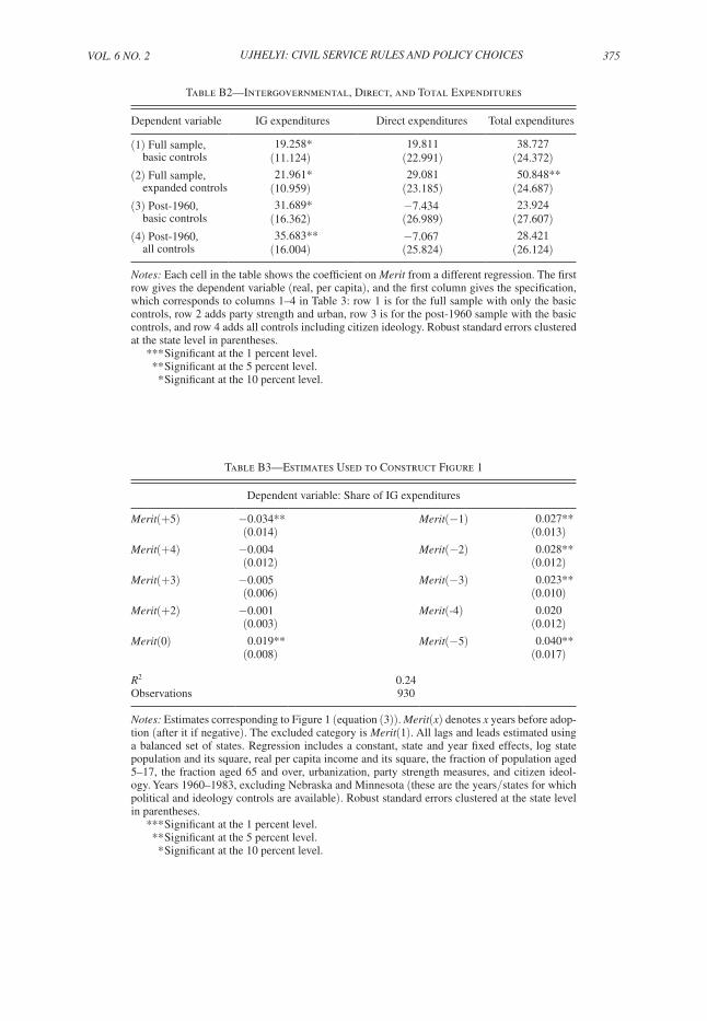
VoL. 6 No. 2 375ujhelyi: Civil ServiCe ruleS and PoliCy ChoiCeS
Table B2—Intergovernmental, Direct, and Total Expenditures
Dependent variable IG expenditures Direct expenditures Total expenditures
(1) Full sample, 19.258* 19.811 38.727 basic controls (11.124) (22.991) (24.372)(2) Full sample, 21.961* 29.081 50.848** expanded controls (10.959) (23.185) (24.687)(3) Post-1960, 31.689* −7.434 23.924 basic controls (16.362) (26.989) (27.607)(4) Post-1960, 35.683** −7.067 28.421 all controls (16.004) (25.824) (26.124)
Notes: Each cell in the table shows the coefficient on merit from a different regression. The first row gives the dependent variable (real, per capita), and the first column gives the specification, which corresponds to columns 1–4 in Table 3: row 1 is for the full sample with only the basic controls, row 2 adds party strength and urban, row 3 is for the post-1960 sample with the basic controls, and row 4 adds all controls including citizen ideology. Robust standard errors clustered at the state level in parentheses.
*** Significant at the 1 percent level. ** Significant at the 5 percent level. * Significant at the 10 percent level.
Table B3—Estimates Used to Construct Figure 1
Dependent variable: Share of IG expenditures
merit(+5) −0.034** merit(−1) 0.027**(0.014) (0.013)
merit(+4) −0.004 merit(−2) 0.028**(0.012) (0.012)
merit(+3) −0.005 merit(−3) 0.023**(0.006) (0.010)
merit(+2) −0.001 merit(-4) 0.020(0.003) (0.012)
merit(0) 0.019** merit(−5) 0.040**(0.008) (0.017)
r2 0.24Observations 930
Notes: Estimates corresponding to Figure 1 (equation (3)). merit(x) denotes x years before adop-tion (after it if negative). The excluded category is merit(1). All lags and leads estimated using a balanced set of states. Regression includes a constant, state and year fixed effects, log state population and its square, real per capita income and its square, the fraction of population aged 5–17, the fraction aged 65 and over, urbanization, party strength measures, and citizen ideol-ogy. Years 1960–1983, excluding Nebraska and Minnesota (these are the years/states for which political and ideology controls are available). Robust standard errors clustered at the state level in parentheses.
*** Significant at the 1 percent level. ** Significant at the 5 percent level. * Significant at the 10 percent level.

376 AmErIcAN EcoNomIc JoUrNAL: EcoNomIc PoLIcy mAy 2014
Table B4—Intergovernmental Expenditures in Additional Spending Categories
Public safety Public safety Administration Administration Education Educationfull sample post-1960 full sample post-1960 full sample post-1960
(1) (2) (3) (4) (5) (6)
merit −0.001 −0.007 −0.002 −0.001 0.017 0.050*(0.008) (0.008) (0.006) (0.005) (0.024) (0.025)
r2 0.20 0.20 0.08 0.07 0.12 0.24
Observations 1,509 1,095 1,463 1,095 1,785 1,095
Natural resources Natural resources Hospitals Hospitals Other Otherfull sample post-1960 full sample post-1960 full sample post-1960
(7) (8) (9) (10) (11) (12)
merit −0.000 0.002 0.001 0.005 0.007 0.009(0.007) (0.010) (0.012) (0.010) (0.019) (0.019)
r2 0.23 0.17 0.40 0.43 0.26 0.25
Observations 1,011 643 1,325 1,095 827 643
Notes: Each column 1–12 presents a separate regression on the fraction of IG spending in a given category within total spending in that category. The category is listed on top of each column. All regressions include a constant, state and year fixed effects, log state population and its square, real per capita income and its square, the fraction of population aged 5–17 and the fraction aged 65 and over, percent urban, and party strength measures. Regressions on the post-1960 sample also control for citizen ideology. Full sample: 46 continental states (excluding Minnesota and Nebraska), available years between 1941–1983. Post-1960: available years between 1960–1983. Robust stan-dard errors clustered at the state level in parentheses.
*** Significant at the 1 percent level. ** Significant at the 5 percent level. * Significant at the 10 percent level.
Table B5—Federal IG Transfers and the Merit System
Dependent variable: Share of revenue from federal IG transfers in total expenditures
Full sample Full sample Post-1960 Post-1960(1) (2) (3) (4)
merit −0.010 −0.008 −0.006 −0.005(0.006) (0.006) (0.006) (0.007)
Party strength Yes YesPercent urban Yes Yescitizen ideology Yes
r2 0.68 0.70 0.44 0.46Observations 1,872 1,785 1,095 1,095
Notes: All regressions include a constant, state and year fixed effects, log state population and its square, real per capita income and its square, the fraction of population aged 5–17, and the fraction aged 65 and over. Party strength variables include Dem. control, rep. control, and Governor’s party. Full sample: 48 continental states, 1941–1983. Post-1960: 1960–1983, exclud-ing Minnesota and Nebraska. Robust standard errors clustered at the state level in parentheses.
*** Significant at the 1 percent level. ** Significant at the 5 percent level. * Significant at the 10 percent level.
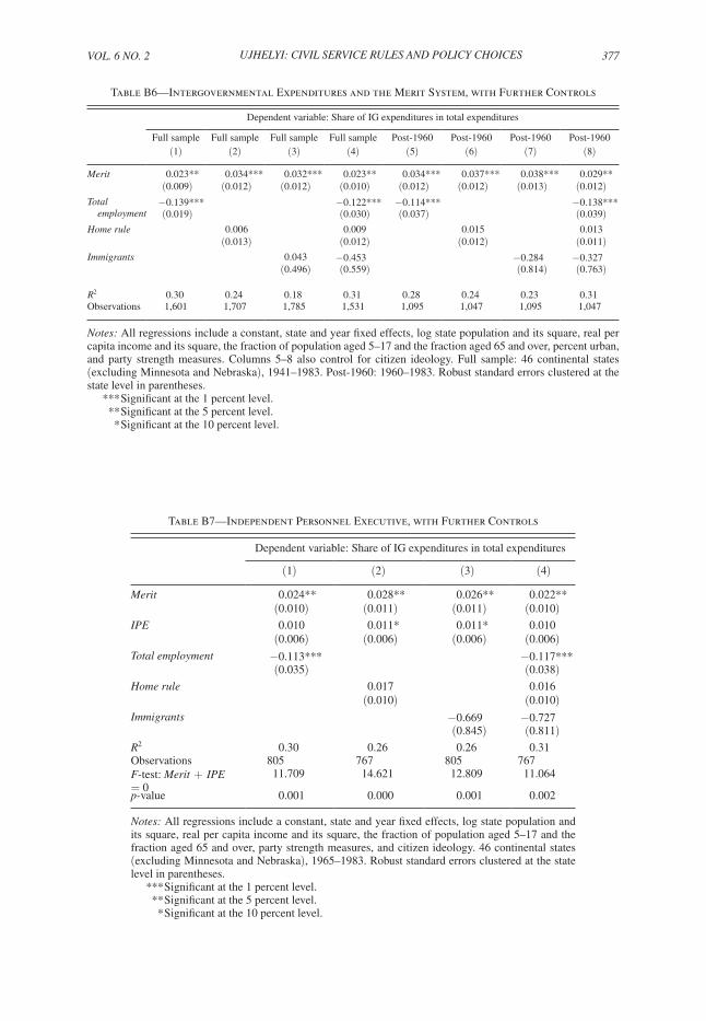
VoL. 6 No. 2 377ujhelyi: Civil ServiCe ruleS and PoliCy ChoiCeS
Table B6—Intergovernmental Expenditures and the Merit System, with Further Controls
Dependent variable: Share of IG expenditures in total expenditures
Full sample Full sample Full sample Full sample Post-1960 Post-1960 Post-1960 Post-1960(1) (2) (3) (4) (5) (6) (7) (8)
merit 0.023** 0.034*** 0.032*** 0.023** 0.034*** 0.037*** 0.038*** 0.029**(0.009) (0.012) (0.012) (0.010) (0.012) (0.012) (0.013) (0.012)
Total −0.139*** −0.122*** −0.114*** −0.138*** employment (0.019) (0.030) (0.037) (0.039)Home rule 0.006 0.009 0.015 0.013
(0.013) (0.012) (0.012) (0.011)Immigrants 0.043 −0.453 −0.284 −0.327
(0.496) (0.559) (0.814) (0.763)
r2 0.30 0.24 0.18 0.31 0.28 0.24 0.23 0.31Observations 1,601 1,707 1,785 1,531 1,095 1,047 1,095 1,047
Notes: All regressions include a constant, state and year fixed effects, log state population and its square, real per capita income and its square, the fraction of population aged 5–17 and the fraction aged 65 and over, percent urban, and party strength measures. Columns 5–8 also control for citizen ideology. Full sample: 46 continental states (excluding Minnesota and Nebraska), 1941–1983. Post-1960: 1960–1983. Robust standard errors clustered at the state level in parentheses.
*** Significant at the 1 percent level. ** Significant at the 5 percent level. * Significant at the 10 percent level.
Table B7—Independent Personnel Executive, with Further Controls
Dependent variable: Share of IG expenditures in total expenditures
(1) (2) (3) (4)
merit 0.024** 0.028** 0.026** 0.022**(0.010) (0.011) (0.011) (0.010)
IPE 0.010 0.011* 0.011* 0.010(0.006) (0.006) (0.006) (0.006)
Total employment −0.113*** −0.117***(0.035) (0.038)
Home rule 0.017 0.016(0.010) (0.010)
Immigrants −0.669 −0.727(0.845) (0.811)
r2 0.30 0.26 0.26 0.31Observations 805 767 805 767F-test: merit + IPE = 0
11.709 14.621 12.809 11.064
p-value 0.001 0.000 0.001 0.002
Notes: All regressions include a constant, state and year fixed effects, log state population and its square, real per capita income and its square, the fraction of population aged 5–17 and the fraction aged 65 and over, party strength measures, and citizen ideology. 46 continental states (excluding Minnesota and Nebraska), 1965–1983. Robust standard errors clustered at the state level in parentheses.
*** Significant at the 1 percent level. ** Significant at the 5 percent level. * Significant at the 10 percent level.

378 AmErIcAN EcoNomIc JoUrNAL: EcoNomIc PoLIcy mAy 2014
REFERENCES
Alesina, Alberto, and Guido Tabellini. 2007. “Bureaucrats or Politicians? Part I: A Single Policy Task.” American Economic review 97 (1): 169–79.
Ansolabehere, Stephen, and James M. Snyder, Jr. 2006. “Party Control of State Government and the Distribution of Public Expenditures.” Scandinavian Journal of Economics 108 (4): 547–69.
Aronson, Albert H. 1979. “State and Local Personnel Administration.” In classics of Public Personnel Policy, edited by Frank J. Thompson, 102–11. Oak Park, IL: Moore Publishing Company.
Bandiera, Oriana, Andrea Prat, and Tommaso Valletti. 2009. “Active and Passive Waste in Government Spending: Evidence from a Policy Experiment.” American Economic review 99 (4): 1278–1308.
Berry, William D., Evan J. Ringquist, Richard C. Fording, and Russell L. Hanson. 1998. “Measuring Citizen and Government Ideology in the American States, 1960–93.” American Journal of Politi-cal Science 42 (1): 327–48.
Besley, Timothy, and Anne Case. 2000. “Unnatural experiments? Estimating the incidence of endog-enous policies.” Economic Journal 110 (467): 672–94.
Besley, Timothy J., and Anne Case. 2003. “Political Institutions and Policy Choices: Evidence from the United States.” Journal of Economic Literature 41 (1): 7–73.
Besley, Timothy, and Stephen Coate. 2003. “Elected vs. Appointed Regulators: Theory and Evidence.” Journal of the European Economic Association 1 (5): 1176–1206.
Burnham, Dean W. 1985. “Partisan Division of American State Governments, 1834–1985.” Conducted by Massachusetts Institute of Technology Inter-University Consortium for Political and Social Research (ICPSR). Ann Arbor: Inter-University Consortium for Political and Social Research [pro-ducer and distributor]. doi:10.3886/ICPSR00016.v1.
Clark, Terry N. 1975. “The Irish Ethic and the Spirit of Patronage.” Ethnicity 2: 305–59.Coate, Stephen, and Brian Knight. 2011. “Government Form and Public Spending: Theory and Evi-
dence from US Municipalities.” American Economic Journal: Economic Policy 3 (3): 82–112.Craig, Steven G., and Robert P. Inman. 1982. “Federal Aid and Public Education: An Empirical Look
at the New Fiscal Federalism.” review of Economics and Statistics 64 (4): 541–52.Dye, Thomas R. 1984. “Party and Policy in the States.” Journal of Politics 46 (4): 1097–1116.Enikolopov, Ruben. 2012. “Politicians, Bureaucrats and Targeted Redistribution.” New Economic
School Working Paper w0148.
Table B8—Results without Education Spending
Dependent variable: Share of IG expenditures in total expenditures
Full sample Full sample Post-1960 Post-1960 Post-1960(1) (2) (3) (4) (5)
merit 0.028** 0.030** 0.020** 0.025*** 0.017(0.011) (0.012) (0.009) (0.009) (0.011)
IPE 0.009(0.008)
Party strength Yes Yes YesPercent urban Yes Yes Yescitizen ideology Yes Yes
r2 0.18 0.20 0.12 0.15 0.22Observations 1,872 1,785 1,095 1,095 805F-test: merit + IPE = 0 5.187p-value 0.028
Notes: Education spending is excluded from all expenditure categories. All regressions include a constant, state and year fixed effects, state population and its square, real per capita income and its square, the fraction of popula-tion aged 5–17, and the fraction aged 65 and over. Party strength variables include Dem. control, rep. control, and Governor’s party. Full sample: 48 continental states, 1941–1983. Post-1960: 1960–1983, excluding Nebraska and Minnesota. Robust standard errors clustered at the state level in parentheses.
*** Significant at the 1 percent level. ** Significant at the 5 percent level. * Significant at the 10 percent level.
VoL. 6 No. 2 379ujhelyi: Civil ServiCe ruleS and PoliCy ChoiCeS
Epstein, David, and Sharyn O’Halloran. 1999. Delegating Powers: A Transaction cost Politics Approach to Policy making under Separate Powers. Cambridge, UK: Cambridge University Press.
Ferreira, Fernando, and Joseph Gyourko. 2009. “Do Political Parties Matter? Evidence From US Cit-ies.” Quarterly Journal of Economics 124 (1): 399–422.
Folke, Olle, Shigeo Hirano, and James M. Snyder, Jr. 2011. “Patronage and Elections in US States.” American Political Science review 105 (3): 567–85.
Freedman, Anne. 1994. Patronage: An American Tradition. Chicago: Nelson-Hall.Hanssen, F. Andrew. 2004. “Is There a Politically Optimal Level of Judicial Independence?” American
Economic review 94 (3): 712–29.Ingraham, Patricia W. 1995. The Foundation of merit: Public Service in American Democracy. Balti-
more: John Hopkins University Press.Iyer, Lakshmi, and Anandi Mani. 2012. “Traveling Agents: Political Change and Bureaucratic Turn-
over in India.” review of Economics and Statistics 94 (3): 723–39.Johnson, Ronald N., and Gary D. Libecap. 1994. The Federal civil Service System and the Problem of
Bureaucracy. Chicago: University of Chicago Press.Kellough, J. Edward, and Lloyd G. Nigro, eds. 2006. civil Service reform in the States. Albany: State
University of New York Press.Knight, Brian. 2002. “Endogenous Federal Grants and Crowd-out of State Government Spending:
Theory and Evidence from the Federal Highway Aid Program.” American Economic review 92 (1): 71–92.
Krane, Dale, Platon N. Rigos, and Melvin B. Hill, Jr. 2001. Home rule in America: A Fifty-State Hand-book. Washington, DC: CQ Press.
Krause, George A., David E. Lewis, and James W. Douglas. 2006. “Political Appointments, Civil Ser-vice Systems, and Bureaucratic Competence: Organizational Balancing and Executive Branch Rev-enue Forecasts in the American States.” American Journal of Political Science 50 (3): 770–87.
Leaver, Clare. 2009. “Bureaucratic Minimal Squawk Behavior: Theory and Evidence from Regulatory Agencies.” American Economic review 99 (3): 572–607.
Lindauer, David L., and Barbara Nunberg, eds. 1996. rehabilitating Government: Pay and Employ-ment reform in Africa. Aldershot, UK: Avebury.
Lockwood, Ben. 2006. “The political economy of decentralization.” In Handbook of Fiscal Federalism, edited by Ehtisham Ahmad and Giorgio Brosio, 33–60. Cheltenham, UK: Edward Elgar.
McCubbins, Mathew D., Roger G. Noll, and Barry R. Weingast. 1987. “Administrative Procedures as Instruments of Political Control.” Journal of Law, Economics, and organization 3 (2): 243–77.
Moe, Terry M. 2006. “Political Control and the Power of the Agent.” Journal of Law, Economics, & organization 22 (1): 1–29.
Orazem, Peter F., and J. Peter Mattila. 1990. “The Implementation Process of Comparable Worth: Winners and Losers.” Journal of Political Economy 98 (1): 134–52.
Rauch, James E. 1995. “Bureaucracy, Infrastructure, and Economic Growth: Evidence from US Cities During the Progressive Era.” American Economic review 85 (4): 968–79.
Rauch, James E., and Peter B. Evans. 2000. “Bureaucratic structure and bureaucratic performance in less developed countries.” Journal of Public Economics 75 (1): 49–71.
Ringquist, Evan J. 1995. “Political Control and Policy Impact in EPA’s Office of Water Quality.” Amer-ican Journal of Political Science 39 (2): 336–63.
Ruhil, Anirudh V. S., and Pedro J. Camões. 2003. “What Lies Beneath: The Political Roots of State Merit Systems.” Journal of Public Administration research and Theory 13 (1): 27–42.
Shafritz, Jay M., David H. Rosenbloom, Norma M. Riccucci, Katherine C. Naff, and Albert C. Hyde. 2001. Personnel management in Government: Politics and Process. 5th ed. New York: Marcel Dekker.
Sorauf, Frank J. 1956. “State Patronage in a Rural County.” American Political Science review 50 (4): 1046–56.
Stahl, O. Glenn. 1956. Public Personnel Administration. 4th ed. New York: Harper and Brothers.Tolchin, Martin, and Susan Tolchin. 1971. To the Victor… Political Patronage from the clubhouse to
the White House. New York: Random House.Ujhelyi, Gergely. 2012. “Civil Service Reform.” Unpublished.Ujhelyi, Gergely. 2014. “Civil Service Rules and Policy Choices: Evidence From US State Gov-
ernments: Dataset.” American Economic Journal: Economic Policy. http://dx.doi.org/10.1257/pol.6.2.338.
United Nations Development Programme (UNDP). 2001. civil Service reform Paper. New York: United Nations Development Programme. http://unpan1.un.org/intradoc/groups/public/documents/un/unpan001183.pdf (accessed August 15, 2012).
380 AmErIcAN EcoNomIc JoUrNAL: EcoNomIc PoLIcy mAy 2014
U.S. Office of Personnel Management. 2003. Biography of an Ideal: A History of the Federal civil Service. Washington, DC. http://www.opm.gov/biographyofanideal/ (accessed August 15, 2012).
Vlaicu, Razvan, and Alex Whalley. 2011. “Hierarchical Accountability in Government: Theory and Evidence.” Unpublished.
Whalley, Alex. 2013. “Elected Versus Appointed Policy-makers: Evidence from City Treasurers.” Jour-nal of Law and Economics 56 (1): 39–81.
Wilson, Woodrow. 1887. “The Study of Administration.” Political Science Quarterly 2 (2): 197–222.Yearley, Clifton K. 1970. The money machines: The Breakdown and reform of Governmental and
Party Finance in the North, 1860–1920. Albany: State University of New York Press.