civl 7/8111 chapter 1 - introduction to fem 1/21 · pdf filea first course in finite elements...

A First Course in Finite Elements

Introduction

The finite element method has become a powerful tool for the numerical solution of a wide range of engineering problems.

Applications range from deformation and stress analysis of automotive, aircraft, building, and bridge structures to field analysis of heat flux, fluid flow, magnetic flux, seepage, and other flow problems.


Introduction

With the advances in computer technology and CAD systems, complex problems can be modeled with relative ease.

Several alternative configurations can be tried out on a computer before the first prototype is built.

All of this suggests that we need to keep pace with these developments by understanding the basic theory, modeling techniques, and computational aspects of the finite element method.


Introduction

In this method of analysis, a complex region defining a continuum is discretized into simple geometric shapes called finite elements.

The material properties and the governing relationships are considered over these elements and expressed in terms of unknown values at element corners.

An assembly process, duly considering the boundary conditions, results in a set of equations.

Solution of these equations gives us the approximate behavior of the continuum.


Piecewise linear function in one dimensions.


Piecewise linear function in two dimensions.

Original two dimensional domain

Discretization of two dimensional domain


CIVL 7/8111 Chapter 1 - Introduction to FEM 1/21

A First Course in Finite ElementsA magnetic problem using

FEM software

Colors indicate that the analyst has set material properties for each zone, in this case a conducting wire coil in orange; a ferromagnetic component (perhaps iron) in light blue; and air in grey.

FEM solution to the problem

The color represents the amplitude of the magnetic flux density, as indicated by the scale in the inset legend, red being high amplitude.








This example duplicates a benchmark problem for time-dependent buoyant flow in porous media. Known as the Elder problem, it follows a laboratory experiment to study thermal convection. This model examines the Elder problem for concentrations through a 2-way coupling of two physics interfaces: Darcy’s Law and Solute Transport.


Chemical vapor deposition (CVD) allows a thin film to be grown on a substrate through molecules and molecular fragments adsorbing and reacting on a surface. This example illustrates the modeling of such a CVD reactor where triethyl-gallium first decomposes, and the reaction products along with arsine (AsH3) adsorb and react on a substrate to form GaAs layers.


A typical automotive exhaust system is a hybrid construction consisting of a combination of reflective and dissipative muffler elements. The reflective parts are normally tuned to remove dominating low-frequency engine harmonics while the dissipative parts are designed to take care of higher-frequency noise. The muffler analyzed in this model, is an example of a complex hybrid muffler in which the dissipative element is created completely by flow through perforated pipes and plates.


This example models the radiation of fan noise from the annular duct of a turbofan aeroengine. When the jet stream exits the duct, a vortex sheet appears along the extension of the duct wall due to the surrounding air moving at a lower speed. The near field on both sides of the vortex sheet is calculated.


Damping elements involving layers of viscoelastic materials are often used for reduction of seismic and wind induced vibrations in buildings and other tall structures. The common feature is that the frequency of the forced vibrations is low. This model studies a forced response of a typical viscoelastic damper. The analysis involves two cases: a frequency response analysis and a time-dependent analysis.


This model treats the free convection and heat transfer of a glass of cold water heated to room temperature. Initially, the glass and the water are at 5 °C and are then put on a table in a room at 25 °C. The nonisothermal flow is coupled to heat transfer using the Heat Transfer module.



The complete analysis consists of two distinct but coupled procedures: a fluid-dynamics analysis with the calculation of the velocity field and pressure distribution in the blood (variable in time and in space) and the mechanical analysis with the deformation of the tissue and artery. The material is assumed to be nonlinear and a hyperelastic model is used.


This model studies the fluid flow through a bending pipe in 3D for the Reynolds number 300 000. Because of the high Reynolds number, the k-epsilon turbulence model is used. Calculations with and without corner smoothing are performed. The results are compared with experimental data.


This model simulates the time-dependent flow past a cylinder. The velocity field magnitude at different time steps is shown.


Historical Background

Basic ideas of the finite element method originated from advances in aircraft structural analysis.

In 1941, Hrenikoff presented a solution of elasticity problems using the “frame work method.”

Courant’s paper, which used piecewise polynomial interpolation over triangular subregions to model torsion problems, appeared in 1943.

Turner et al. (1956) derived stiffness matrices for truss, beam, and other elements.

The term “finite element” was first coined and used by Clough in 1960.



In the early 1960s, engineers used the method for approximate solution of problems in stress analysis, fluid flow, heat transfer, and other areas.

A book by Argyris in 1955 on energy theorems and matrix methods laid a foundation for further developments in finite element studies.

The first book on finite elements by Zienkiewicz and Chung was published in 1967.

In the late 1960s and early 1970s, finite element analysis was applied to nonlinear problems and large deformations.



Mathematical foundations were laid in the 1970s.

New element development, convergence studies, and other related areas fall in this category.

Today, developments in mainframe computers and availability of powerful microcomputers have brought this method within reach of students and engineers working in small industries.


Role of Computers in Finite Element Methods

Until the early 1950s, matrix methods and the associated finite element method were not readily adaptable for solving complicated problems because of the large number of algebraic equations that resulted.

Hence, even though the finite element method was being used to describe complicated structures, the resulting large number of equations associated with the finite element method of structural analysis made the method extremely difficult and impractical to use.

With the advent of the computer, the solution of thousands of equations in a matter of minutes became possible.

Step 1 - Discretize and Select Element Types


Step 1 involves dividing the body into an equivalent system of finite elements with associated nodes and choosing the most appropriate element type.

The total number of elements used and their variation in size and type within a given body are primarily matters of engineering judgment.

The elements must be made small enough to give usable results and yet large enough to reduce computational effort.

Small elements (and possibly higher-order elements) are generally desirable where the results are changing rapidly, such as where changes in geometry occur, whereas large elements can be used where results are relatively constant.


Primary line elements consist of bar (or truss) and beam elements.

They have a cross-sectional area but are usually represented by line segments.

The simplest line element (called a linear element) has two nodes, one at each end, although higher-order elements having three nodes or more (called quadratic, cubic, etc. elements) also exist.



The basic two-dimensional (or plane) elements are loaded by forces in their own plane (plane stress or plane strain conditions). They are triangular or quadrilateral elements.

The simplest two-dimensional elements have corner nodes only (linear elements) with straight sides or boundaries although there are also higher-order elements, typically with mid-side nodes (called quadratic elements) and curved sides.






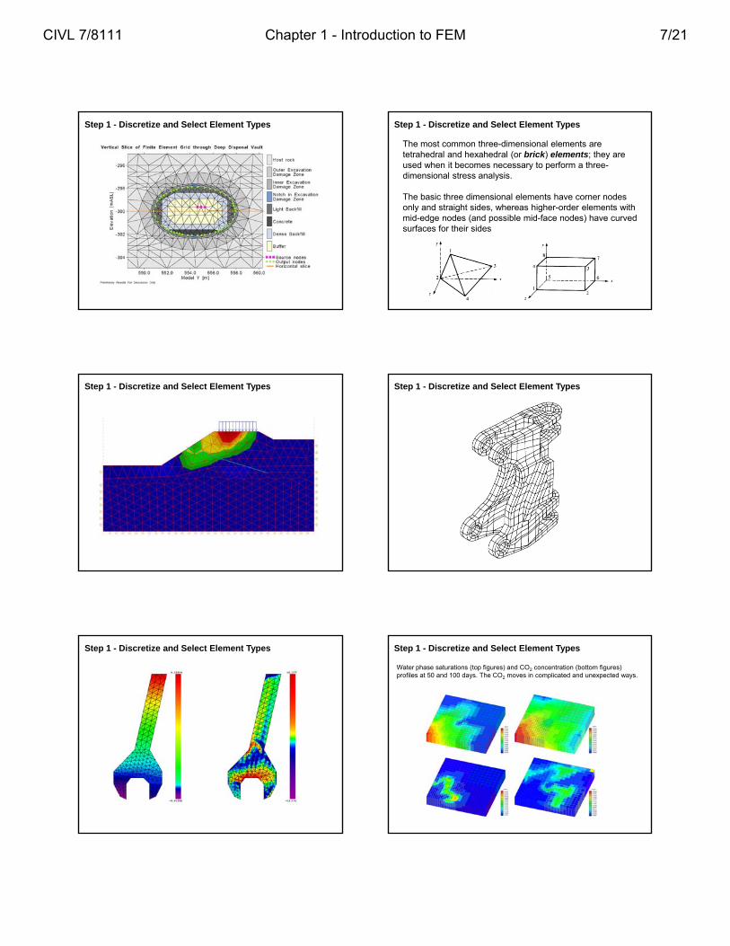
The most common three-dimensional elements are tetrahedral and hexahedral (or brick) elements; they are used when it becomes necessary to perform a three-dimensional stress analysis.

The basic three dimensional elements have corner nodes only and straight sides, whereas higher-order elements with mid-edge nodes (and possible mid-face nodes) have curved surfaces for their sides



Water phase saturations (top figures) and CO2 concentration (bottom figures) profiles at 50 and 100 days. The CO2 moves in complicated and unexpected ways.





As a consequence of our changing climate, large efforts have been made to understand the social risks of storm surges (hypothesized to increase in frequency in warmer climate scenarios) and sea level rise in coastal areas. Of particular interest is the role that wetlands and coastal marshes play in storm surges and flooding events.



The axisymmetric element is developed by rotating a triangle or quadrilateral about a fixed axis located in the plane of the element through 360°.

This element can be used when the geometry and loading of the problem are axisymmetric.





Consider the problem of the axial deformation of a linearly elastic bar under an axial load P at x = L and distributed external load q(x).

The cross-sectional area, A(x), the modulus of elasticity, E, and the mass density, (x), are given.

P = external loadq(x) = distributed loadu(x) = axial displacementu(x)

x

L

P

q(x)


Let’s assume that the variation of the loads, P(x) and q(x), and the cross-sectional area, A(x), are complicated and the exact solution to the above equation cannot be found.

The basic concept of FEM is to cut the problem up into a series of simpler discrete problems and relate the parts to each other to model the continuous material. A possible example of a discrete model of the bar is:

u(x)

x

L

P q(x)

1 2 3 4 5


Discrete means essentially that we are willing to accept a model that will yield information about the dependent variables at a finite number of points, referred to as nodes, within the interval 0 ≤ x ≤ L.

Each node is assigned a displacement ui, i = 1 to 5. The problem has been converted from a continuous model of infinite degrees of freedom to one with a finite number of degrees of freedom, in this case n = 5.

u(x)

x

L

P q(x)

1 2 3 4 5


The elastic effects of the discrete parts of the bar may be represented as elements.

In our problem, the elongation of an axial bar under an axial load is represented by:

avg

Ple

A E avgA E

P e kel

u(x)

x

L

P q(x)

1 2 3 4 5


Therefore, an elastic bar of length l is equivalent to a simple linear spring.

The stiffness associated with each “element” will be a different value since Aavg varies from node to node. Let’s approximate the stiffness, k, by taking:

1

2i i

i

A A Ek

l

1

2i i

avg

A AA

u(x)

x

l1

P q(x)

1 2 3 4 5

l2 l3 l4

AE1 AE2 AE3 AE4



Equivalent systems of springs connecting each set of nodes are referred to as elements.

An element generally describes some basic physical property of the system. In the case of the axial bar, the relationship between force and displacement is:

1i i i i i iF k e k u u

Another important physical parameter associated with the element is the mass.

There are several ways to distribute the mass. Keeping the concept of the element we have developed so far, let’s consider the mass of the portion of the bar between nodes i and i+1 defining element i.


Keeping the concept of the element we have developed so far, let’s consider the mass of the portion of the bar between nodes iand i+1 defining element i.

One method of distributing the mass is to average the mass over the element and divide it equally between the two nodes defining the element. The average mass intensity is:

1 1* 1

2 2i i i i i i

x A x x A x m mm

u(x)

x

l1

i i+1

l2 l3 l4



Therefore the discrete lumped mass system is:

1 2 1

1 4

m m lM

M1 M2 M3 M4 M5

1 2 1 2 3 2

2 4 4

m m l m m lM

2 3 2 3 4 3

3 4 4

m m l m m lM

3 4 3 4 5 4

4 4 4

m m l m m lM

4 5 4

5 4

m m lM

u(x)

x

l1

i i+1

l2 l3 l4



The sum of the masses should approximately satisfy the following relationship:

0

L

iM x A x dx

u(x)

x

l1

i i+1

l2 l3 l4



Identical to the lumping technique used for mass, we will take the average of the loading intensity:

1* 1

2 2i i i i

q x q x q qq

u(x)

x

l1

i i+1

l2 l3 l4



Therefore the discrete lumped loading is:

1 2 1

1 4

q q lQ

Q1 Nodal loads Qi

Q2 Q3 Q4 Q5

1 2 1 2 3 2

2 4 4

q q l q q lQ

2 3 2 3 4 3

3 4 4

q q l q q lQ

3 4 3 4 5 4

4 4 4

q q l q q lQ

4 5 4

5 4

q q lQ

u(x)

x

l1

i i+1

l2 l3 l4




The sum of the nodal loads should approximately satisfy the following relationship:

0

L

iQ q x dx

u(x)

x

l1

i i+1

l2 l3 l4



The final discrete model for this system with springs, masses, and loads would be:

Q1 Q2 Q3 Q4 Q5

M1 M2 M3 M4 M5k1 k2 k3 k4

u(x)

x

l1

i i+1

l2 l3 l4

Step 2 - Select a Displacement Function

This completes the process of converting the continuous system into what is hoped to be a equivalent discrete system.

The discretization should be implicit in the representation of the mass, elastic properties, and loads.

Whether the axial model is continuous or discrete, equilibrium of the system (Newton’s second law) must be satisfied.

The remaining steps of assembly, constraints, solution, and computation of derived variables can be best illustrated in an example.

Equilibrium of a Spring Mass System - Vectorial Approach

Consider a typical spring-mass system, where each spring ki is assumed to behave in a linear way ( F = kx ) and the loads Pi

are applied slowly to the system so that the problem is static.

The nodal displacements and the corresponding internal forces for an element are:

fi

ui ui+1

ki

fi+1

1 1 1i i i i i i i if k u u f k u u

1 1

1 1 1 1

ori ie e e

i i

f k k uf k u

f k k u

Equilibrium of a Spring Mass System - Vectorial Approach

where ke is called the element stiffness matrix, fe is the element force, and ue is the element displacement vector.

This equation is a statement of the spring relationship F = kx on the elemental level.

The individual ke can be assembled into the global stiffness matrix which represents the physical nature of the entire system.

e e ef k u

Introduction

Example - Consider a uniform square bar under a distributed loading. Use five equally-spaced nodes to discretize the following problem. Solve for the displacement at each node.

The discretization of the bar is:

21 in.A

29,000E ksiu(x)

x

10 ft.

10 kips

u(x)

x

10 kips

1 2 3 4 5

2.5 ft. 2.5 ft. 2.5 ft. 2.5 ft.

1 1

1 1 1 1

i i

i i

f k k u

f k k u

e e ef k u


Introduction

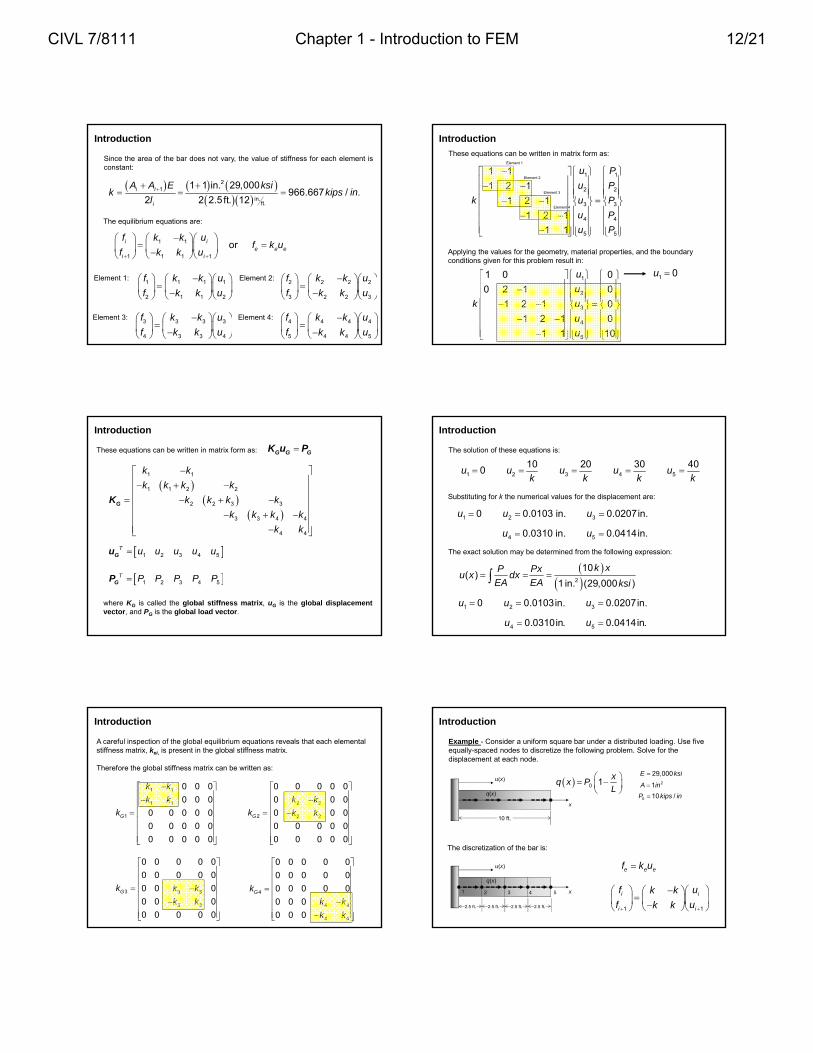
Since the area of the bar does not vary, the value of stiffness for each element isconstant:

21

in.ft.

1 1 in. 29,000966.667 / .

2 2 2.5 ft. 12i i

i

A A E ksik kips in

l

The equilibrium equations are:

1 1

1 1 1 1

ori ie e e

i i

f k k uf k u

f k k u

1 1 1 1

2 1 1 2

f k k u

f k k u

Element 1:

3 33 3

3 34 4

k kf u

k kf u

Element 3:

2 22 2

3 32 2

f uk k

f uk k

Element 2:

4 44 4

5 54 4

f uk k

f uk k

Element 4:

Introduction

These equations can be written in matrix form as:

where KG is called the global stiffness matrix, uG is the global displacementvector, and PG is the global load vector.

G G GK u P

1 1

1 1 2 2

2 2 3 3

3 3 4 4

4 4

k k

k k k k

k k k k

k k k k

k k

GK

1 2 3 4 5T P P P P PGP

1 2 3 4 5T u u u u uGu

Introduction

A careful inspection of the global equilibrium equations reveals that each elemental stiffness matrix, kei, is present in the global stiffness matrix.

Therefore the global stiffness matrix can be written as:

1 1

1 1

1

0 0 0

0 0 0

0 0 0 0 0

0 0 0 0 0

0 0 0 0 0

G

k k

k k

k

2 2

2 2 2

0 0 0 0 0

0 0 0

0 0 0

0 0 0 0 0

0 0 0 0 0

G

k k

k k k

3 3 3

3 3

0 0 0 0 0

0 0 0 0 0

0 0 0

0 0 0

0 0 0 0 0

Gk k k

k k

4

4 4

4 4

0 0 0 0 0

0 0 0 0 0

0 0 0 0 0

0 0 0

0 0 0

Gk

k k

k k

Introduction

These equations can be written in matrix form as:

Applying the values for the geometry, material properties, and the boundary conditions given for this problem result in:

1 1

2 2

3 3

4 4

5 5

1 1

1 2 1

1 2 1

1 2 1

1 1

u P

u P

k u P

u P

u P

1

2

3

4

5

1 0 0

0 2 1 0

1 2 1 0

1 2 1 0

1 1 10

u

u

k u

u

u

Element 1

Element 2

Element 3

Element 4

1 0u

Introduction

The solution of these equations is:

Substituting for k the numerical values for the displacement are:

1 2 3 4 5

10 20 30 400u u u u u

k k k k

The exact solution may be determined from the following expression:

2

10( )

1 in. (29,000 )

k xP Pxu x dx

EA EA ksi

1 2 30 0.0103 in. 0.0207in.u u u

4 50.0310 in. 0.0414in.u u

1 2 30 0.0103in. 0.0207in.u u u

4 50.0310in. 0.0414in.u u

Introduction

Example - Consider a uniform square bar under a distributed loading. Use five equally-spaced nodes to discretize the following problem. Solve for the displacement at each node.


0 1x

q x PL

29,000E ksi21A in

0 10 /P kips in

u(x)

x

10 ft.

q(x)

u(x)

x1 2 3 4 5

2.5 ft. 2.5 ft. 2.5 ft. 2.5 ft.

q(x)

e e ef k u

1 1

i i

i i

f uk k

f uk k


Introduction

To handle the distributed load, we will lump the loads into each node. The averageloading intensity is computed as:


1* 1

2 2i i i i

q x q x q qq

0( )2

L

io

P LQ q x dx

Introduction

The individual values for the distributed lumped loads are:

1 2 1

1 4

q q lQ

1 00q x P

0 1x

q x PL

2 0

2.52.5 ft. 1

10q x P 00.75P

1 2 1 01

1.75

4 4 4

q q l P LQ 07

64

P L 028

256

P L

Introduction


1 2 1 01

28

4 256

q q l P LQ

1 2 1 2 3 2 02

48

4 4 256

q q l q q l P LQ

2 3 2 3 4 3 03

32

4 4 256

q q l q q l P LQ

3 4 3 4 5 4 04

16

4 4 256

q q l q q l P LQ

4 5 4 05

4

4 256

q q l P LQ

Introduction

Applying the values for the geometry, material properties, and loading distributionconditions results in:

1

2

03

4

5

1 1 28

1 2 1 48

1 2 1 32256

1 2 1 16

1 1 4

u

uP L

k u

u

u

Element 1

Element 2

Element 3

Element 4

Introduction

Applying the values for the geometry, material properties, loading distribution, andthe boundary conditions results in:

1

2

03

4

5

1 0 0

0 2 1 48

1 2 1 32256

1 2 1 16

1 1 4

u

uP L

k u

u

u


2 20 0

1 2 30 100 1521,024 1,024

P L P Lu u u

AE AE

2 20 0

4 5172 1761,024 1,024

P L P Lu u

AE AE

1 0u

Introduction

Substituting the numerical values for P0, L, and k results in :

1 2 30 0.4849in. 0.7371in.u u u

4 50.8341in. 0.8534in.u u


2

0 0 1( ) 1 '2

x xAEu x P dx P x C

L L

0 01( ) ( ) '

( )

uu x q x dx dx

EA x AEu L P

010

2

P LAEu L C


Introduction


1 2 30 0.4849in. 0.7371in.u u u

4 50.8341in. 0.8534in.u u


3 220 1 1 1

( )6 2 2

P L x x xu x

AE L L L

1 2 30 0.4784in. 0.7241in.u u u

4 50.8147in. 0.8276in.u u

Introduction

Example - Repeat the previous problem using nine equally-spaced nodes (8 elements) to discretize the problem. Solve for the displacement at each node.


0 1x

q x PL

29,000E ksi21A in

0 10 /P kips in

u(x)

x

10 ft.

q(x)

e e ef k u

1 1

1 1 1 1

i i

i i

f k k u

f k k u

u(x)

x1 2 3 4 5

q(x)

6 7 8 9

Introduction

To handle the distributed load, we will lump the loads into each node. The averageloading intensity is computed as:


1* 1

2 2i i i i

q x q x q qq

0( )2

L

io

P LQ q x dx

Introduction


1 2 1 01

14

4 256

q q l P LQ

1 2 1 2 3 2 02

28

4 4 256

q q l q q l P LQ

0 0 03 4 524 20 16

256 256 256

P L P L P LQ Q Q

0 0 0 06 7 8 912 8 4

256 256 256 256

P L P L P L P LQ Q Q Q

Introduction

Applying the values for the geometry, material properties, and loading given in thisproblem results in:

1

2

3

4

05

6

7

8

9

1 1 0 0 0 0 0 0 0 14

1 2 1 0 0 0 0 0 0 28

0 1 2 1 0 0 0 0 0 24

0 0 1 2 1 0 0 0 0 20

0 0 0 1 2 1 0 0 0 16256

0 0 0 0 1 2 1 0 0 12

0 0 0 0 0 1 2 1 0 8

0 0 0 0 0 0 1 2 1 4

0 0 0 0 0 0 0 1 1 1

u

u

u

uP L

k u

u

u

u

u

Element 1

Element 2

Element 3

Element 4

Element 8

Element 5

Element 6

Element 7

Introduction

Applying the boundary condition results in:

1

2

3

4

05

6

7

8

9

1 0 0 0 0 0 0 0 0 0

0 2 1 0 0 0 0 0 0 28

0 1 2 1 0 0 0 0 0 24

0 0 1 2 1 0 0 0 0 20

0 0 0 1 2 1 0 0 0 16256

0 0 0 0 1 2 1 0 0 12

0 0 0 0 0 1 2 1 0 8

0 0 0 0 0 0 1 2 1 4

0 0 0 0 0 0 0 1 1 1

u

u

u

uP L

k u

u

u

u

u

1 0u


Introduction


2 20 0

1 3 50 198 3002,048 2,048

P L P Lu u u

AE AE

2 20 0

7 9338 3442,048 2,048

P L P Lu u

AE AE


1 3 50 0.4801in. 0.7274in.u u u

7 90.8195in. 0.8341in.u u


1 2 30 0.4784in. 0.7241in.u u u

4 50.8147in. 0.8276in.u u

Introduction

PROBLEM #1 - Consider a square bar subjected to a series of concentrated loads. Use five equally-spaced nodes to discretize the following problem. Solve for the displacement at each node and compare to the exact solution.

25 2x

A x inL

29,000E ksi

25l in

5P kips

u(x)

x

l

4P

l l l

P 2P 3P

Introduction

PROBLEM #2 - Repeat PROBLEM #1 using twice the number of elements. Compare your results with those obtained in PROBLEM #1 and the exact solution. Explain any differences in the solutions.

25 2x

A x inL

29,000E ksi

25l in

5P kips

u(x)

x

l

4P

l l l

P 2P 3P

Introduction

PROBLEM #3 - Consider a uniform square bar under a distributed loading. Use five equally-spaced nodes to discretize the following problem. Solve for the displacement at each node.

2

0 1x

q x PL

29,000ksiE 21 in.A

0 5 kips/in.P u(x)

x

100 in.

q(x)

PLANE TRUSS STRUCTURES

From your experience in structural analysis you are aware of structural elements or members called “two force members”.

These elements are pin connected and transmit only an axial force. There is no shear, bending, or torsional loads transmitted by these members in a structure.

A structure composed of two-force members which behaves elastically may be replaced by a system of connected “springs”. Consider a single two-force member:

1i i i iP k u u 1 1i i i iP k u u

iP 1iP

iu 1iu

x

y


The spring stiffness constant ki is (AE/L )i, where A is an area, E is the modulus of elasticity, and L is the length of the member.

Consider a plane truss with four bars or members or elements:

2P

1P

Although each member in the truss will elongate (or contract) and transmit a tensile (or compressive) load, the displacements and the forces are in different directions.


Although each member in the truss will elongate (or contract) and transmit a tensile (or compressive) load, the displacements and the forces are in different directions.


, , , global coordinatesX YX Y F F

2 2,XF U

2 2,YF V

1 1,YF V

1 1,XF U , , , element coordinatesx yx y f f

2 2,xf u2 2,yf v

1 1,yf v

1 1,xf u

X

Y

xy


The global force components may be related to the elemental force componentsby:

1 1 1 1 1 1X x y Y x yF f cos f sin F f sin f cos


2 2,XF U

2 2,YF V

1 1,YF V


2 2,xf u2 2,yf v

1 1,yf v

1 1,xf u

X

Y

xy


The displacements may be related in a similar fashion:

1 1 1 1 1 1U u cos v sin V u sin v cos


2 2,XF U

2 2,YF V

1 1,YF V


2 2,xf u2 2,yf v

1 1,yf v

1 1,xf u

X

Y

xy


In matrix form these quantities can be expressed as:

The global force and global displacement vectors and R is a transformation matrix for rotation of an axis ( R-1 = RT ).

A set of similar quantities can be written for the other end of the element

1 1 1 1F Rf U Ru

111 1

11

cos sin

sin cosxX

yY

fFF f R

fF

1 11 1

1 1

U uU u

V v


The stiffness matrix for the axial element in the elemental or local coordinates is:

Rewriting the elemental forces-displacement relationship for both x and ycomponents:

1 1

2 2

x

x

f uk k

f uk k

1 1

1 1

2 2

2 2

0 0

0 0 0 0

0 0

0 0 0 0

x

y

x

y

f uk k

f v

f uk k

f v

Notice the second and fourth equations reflect the fact that only axial loads, in the x-direction locally, are possible in the absence of bending, shear, or torsion.


These equations may be written in partitioned form as:

To convert these relationships to global coordinates (X, Y) we apply the coordinate transformation R.

1 11 12 1 1 11 1 12 2

2 21 22 2 2 21 1 22 2

f k k u f k u k u

f k k u f k u k u

1 11 1 1 1f R F u R U

1 1 12 21 1 22 2 2 21 1 22 2f k u k u R F k R U k R U

1 1 11 11 1 12 2 1 11 1 12 2f k u k u R F k R U k R U

1 11 11 1 12 2F Rk R U Rk R U

1 12 21 1 22 2F Rk R U Rk R U

Multiply both side by R:



Since R-1 = RT

In a more convenient form:

Writing these equations in still a more compact form gives

=

T T1 111 12

T T2 221 22

F URk R Rk R

F URk R Rk R

0 0=

0 0

T1 11 12 1

T2 21 22 2

F k k UR R

F k k UR R

0

0

T R

F TkT U KU TR

where K is the global stiffness matrix for a single two-force member or element.


Substituting the values of R and k and performing the multiplication gives:

In this case, K is the global stiffness matrix for a single truss element.

In a structure composed of two-force elements, say a truss, we would have to assembly the element global matrices into a global matrix for the entire system.

Before we discuss any problems or work any examples, let’s look at the effect of discretization on the form of the system stiffness matrix.

2 2

2 2

2 2

2 2

cos

sink

K


Consider the following two ways to number the nodes of the same truss:

5 6 7

1 2 3 4

2 4 6

1 3 5 7

Number Scheme #2

Number Scheme #1


Consider the following two ways to number the nodes of the same truss:

5 6 7

1 2 3 4

2 4 6

1 3 5 7

From these idealizations, it is clear that the second numbering scheme produces aglobal matrix that has a smaller band width.

Generally, this type of symmetry results in quicker solutions and a reduction in therequired memory or storage capacity.

The half-band width of a symmetric set of equations for row i and column j of thelast non-zero entry may be computed as:

1i

nb j i

where NB (half the band width) is the maximum of the (nb)i over all rows.


SOLUTION PROCEDURE

1. Define a discretization of the truss (recall the node numbering scheme we discussed above)

2. Assemble the elemental stiffness and load matrices. Each element matrix should be transformed into the global system as previously described.

3. Apply boundary conditions or constraints to the system equations

4. Solve the system equations

5. Compute the forces in the members. Recall the force displacement relationship

Tf ku kT U

1 1 2 1 2 1 0x yf k U U cos V V sin f

2 1 2 1 2 2 0x yf k U U cos V V sin f


Example - Develop the element stiffness matrices and system equations for the plane truss below. Assume the stiffness of each element is constant. Use the numbering scheme indicated. Solve the equations for the displacements and compute the member forces.

STEP 1. The node numbering is given in the diagram above (Note that this is theoptimum numbering configuration).

All elements have a constant k

1

2

3



STEP 2. Develop the element information

Compute the elemental stiffness matrix for each element. The general form of thematrix is:

Member Node 1 Node 2 Elemental Stiffness

1 1 2 k 0

2 2 3 k 3/4

3 1 3 k /2

2 2

2 2

2 2

2 2

cos

sink

K


For element 1:

1 1 2 2

1

1

2

2

1 0 1 0

0 0 0 0

1 0 1 0

0 0 0 0

U V U V

U

VK k

U

V

For element 3:For element 2:

2 2

2 2

2 2

2 2

cos

sink

K

2 2 3 3

2

2

3

3

1 1 1 1

1 1 1 1

2 1 1 1 1

1 1 1 1

U V U V

U

VkK

U

V

1 1 3 3

1

1

3

3

0 0 0 0

0 1 0 1

0 0 0 0

0 1 0 1

U V U V

U

VK k

U

V


Assemble the global system matrix by superimposing the elemental global matrices.

1 1 2 2 3 3

1

1

2

2

3

3

2 0 2 0 0 0

0 2 0 0 0 2

2 0 3 1 1 1

2 0 0 1 1 1 1

0 0 1 1 1 1

0 2 1 1 1 3

U V U V U V

U

V

UkV

U

V

K

Element 1

Element 2Element 3


The unconstrained (no boundary conditions satisfied) equations are:

1

1

2 1

2 2

3

3

2 0 2 0 0 0 0

0 2 0 0 0 2 0

2 0 3 1 1 1

2 0 0 1 1 1 1

0 0 1 1 1 1

0 2 1 1 1 3 0

U

V

U PkV P

U P

V


STEP 3. The displacement at nodes 1 and 3 are zero in both directions. Applying these conditions to the system equations gives:

1

1

2 1

2 2

3

3

1 0 0 0 0 0 0

0 1 0 0 0 0 0

0 0 3 1 0 0

2 0 0 1 1 0 0

0 0 0 0 1 0 0

0 0 0 0 0 1 0

U

V

U PkV P

U

V


STEP 4. Solving this set of equations is fairly easy. The solution is:

STEP 5. Using the force-displacement relationship the force in each member maybe computed.

3 30 0U V

1 2 1 21 1 2 2

30 0

P P P PU V U V

k k

Member (element) 1

1 21 2 1 1 0x y

P Pf k P P f

k

1 22 1 2 2 0x y

P Pf k P P f

k




Member (element) 2

1 2 1 22 2

31 12

2 2x

P P P Pf k P

k k

1 2 1 23 2

31 12

2 2x

P P P Pf k P

k k

2 0yf

3 0yf



Member (element) 33 3

1 1

0 0

0 0x y

x y

f f

f f

X

Y

Element 1 2 1 2xf P P 1 1 2xf P P

x

Element 3

3 0xf

1 0xf

xElement 2

3 22xf P

2 22xf P

x



STEP 1. A node numbering configuration is given (note that this is the optimumnumbering configuration).

All elements have a constant value of k



STEP 1. A node numbering configuration is given (note that this is the optimumnumbering configuration).

Element number

Node number

4

4


STEP 2. Develop the element information

Compute the elemental stiffness matrix for each element. The general form of thematrix is:

Element Node 1 Node 2 Elemental Stiffness 1 1 2 k /4

2 2 3 k 3/2

3 1 3 k 0

4 2 4 k 7/4

5 3 4 k 0

2 2

2 2

2 2

2 2

cos

sink

K


For elements 1 and 2:

1 1 2 2 2 2 3 3

21

21

32

32

1 1 1 1 0 0 0 0

1 1 1 1 0 2 0 2

2 1 1 1 1 2 0 0 0 0

1 1 1 1 0 2 0 2

U V U V U V U V

UU

VVk kK K

UU

VV

For elements 3 and 4:

1 1 3 3 2 2 4 4

1 2

1 2

3 4

3 4

2 0 2 0 1 1 1 1

0 0 0 0 1 1 1 1

2 2 0 2 0 2 1 1 1 1

0 0 0 0 1 1 1 1

U V U V U V U V

U U

V Vk kK K

U U

V V



For element 5:

Assemble the global system matrix by superimposing the elemental global matrices.

3 3 4 4

3

3

4

4

2 0 2 0

0 0 0 0

2 2 0 2 0

0 0 0 0

U V U V

U

VkK

U

V

1 1 2 2 3 3 4 4

1

1

2

2

3

3

4

4

3 1 1 1 2 0 0 0

1 1 1 1 0 0 0 0

1 1 2 0 0 0 1 1

1 1 0 4 0 2 1 1

2 2 0 0 0 4 0 2 0

0 0 0 2 0 2 0 0

0 0 1 1 2 0 3 1

0 0 1 1 0 0 1 1

U V U V U V U V

U

V

U

VkU

V

U

V

K


The unconstrained (no boundary conditions satisfied) equations are:

1

1

2

2

3

3

4

4

3 1 1 1 2 0 0 0 0

1 1 1 1 0 0 0 0 0

1 1 2 0 0 0 1 1

1 1 0 4 0 2 1 1 0

2 2 0 0 0 4 0 2 0 0

0 0 0 2 0 2 0 0 2

0 0 1 1 2 0 3 1 0

0 0 1 1 0 0 1 1 0

U

V

U P

VkU

V P

U

V


STEP 3. Apply the boundary conditions to the system equations:

1

1

2

2

3

3

4

4

1 0 0 0 0 0 0 0 0

0 1 0 0 0 0 0 0 0

0 0 2 0 0 0 0 0

0 0 0 4 0 2 0 0 0

2 0 0 0 0 4 0 0 0 0

0 0 0 2 0 2 0 0 2

0 0 0 0 0 0 1 0 0

0 0 0 0 0 0 0 1 0

U

V

U P

VkU

V P

U

V


STEP 4. Solving this set of equations is fairly easy. The solution is:


Member (element) 1

1 1 2 2

20 0

P PU V U V

k k

3 3 4 4

40 0 0

PU V U V

k

2

1 12

2 2 2x

Pf P P

1

1 12

2 2 2x

Pf P P



Member (element) 2

2 32 4 2 2 4 2x xf P P f P P

Member (element) 3

1 30 0x xf f

Member (element) 4

2

1 1 32

2 2 2x

Pf P P

4

1 1 32

2 2 2x

Pf P P



Member (element) 5

3 40 0x xf f

Element Node 1 Node 2 Unode 1 Unode2 Vnode 1 Vnode 2 fx

1 1 2 0 P/k 0 -2P/k 0.707P (C)

2 2 3 P/k 0 -2P/k -4P/k 2P (T)

3 1 3 0 0 0 -4P/k 0

4 2 4 P/k 0 -2P/k 0 2.12P (C)

5 3 4 0 0 -4P/k 0 0



PROBLEM #4 - Develop the element stiffness matrices and system equations for the plane truss below. Assume the stiffness of each element is constant. Use the numbering scheme indicated. Solve the equations for the displacements and compute the member forces.

Element number

Node number

4

4

All elements have a constant value of k


PROBLEM #5 - Develop the element stiffness matrices and system equations for the plane truss below. Assume the stiffness of each element is constant. Use the numbering scheme indicated. Solve the equations for the displacements and compute the member forces.

4P

P

45o 45o

4P

P

31 4

2

1

2

3 5

4

P

2k

k k

2k

3k

P

Element number

Node number

4

4


PROBLEM #6 - Consider the following two-dimensional plane truss. For the given node numbering scheme, determine the displacements of each node and the member forces. Check your results by using the method of sections and the method of joints from static analysis. For computational purposes assume a P = 10 kips, E = 29,000 ksi, L = 10 ft., and A = 4 in.2.

End of Introduction


civl 7/8111 chapter 1 - introduction to fem 1/21 · pdf filea first course in finite elements...

Documents