Published as: Cornelis Stal, Christian Briese, Philippe De Maeyer, Peter Dorninger, Timothy Nuttens, Norbert Pfeifer

& Alain De Wulf (2014) Classification of airborne laser scanning point clouds based on binomial logistic regression

analysis, International Journal of Remote Sensing, 35(9), 3219-3236.

Classification of airborne laser scanning point clouds based on binomial logistic

regression analysis

Cornelis Stala*, Christian Brieseb,c, Philippe De Maeyera, Peter Dorningerb,d, Timothy Nuttensa, Norbert Pfeiferb, and Alain De Wulfa

aDepartment of Geography, Ghent University, Ghent, Belgium; bDepartment of Geodesy and Geoinformation, Vienna University of Technology, Vienna, Austria; cDepartment of Archaeological Remote Sensing, LBI for Archaeological

Prospection & Virtual Archaeology, Vienna, Austria; d4D-IT GmbH, Pfaffstätten, Austria

This article presents a newly developed procedure for the classification of airborne laser scanning (ALS) point clouds, based on binomial logistic regression analysis. By using a feature space containing a large number of adaptable geometrical parameters, this new procedure can be applied to point clouds covering different types of topography and variable point densities. Besides, the procedure can be adapted to different user requirements. A binomial logistic model is estimated for all a priori defined classes, using a training set of manually classified points. For each point, a value is calculated defining the probability that this point belongs to a certain class. The class with the highest probability will be used for the final point classification. Besides, the use of statistical methods enables a thorough model evaluation by the implementation of well-founded inference criteria. If necessary, the interpretation of these inference analyses also enables the possible definition of more sub-classes. The use of a large number of geometrical parameters is an important advantage of this procedure in comparison with current classification algorithms. It allows more user modifications for the large variety of types of ALS point clouds, while still achieving comparable classification results. It is indeed possible to evaluate parameters as degrees of freedom and remove or add parameters as a function of the type of study area. The performance of this procedure is successfully demonstrated by classifying two different ALS point sets from an urban and a rural area. Moreover, the potential of the proposed classification procedure is explored for terrestrial data.

1. Introduction

Airborne laser scanning (ALS) is a popular 3D data acquisition technique for urban and rural environmental modelling (Doneus et al. 2008; Oude Elberink and Vosselman 2011; Stal et al. 2013). It allows the measurement of a 3D point cloud that represents the area of interest, by irradiating it with a laser beam from an airborne platform (Baltsavias 1999). One of the main requirements when dealing with an ALS point cloud is an accurate and efficient point classification or filtering (Briese 2010; Pfeifer and Mandlburger 2008). Classification, on the one hand, is the process where points are assigned to a certain class based on common properties. Filtering, on the other hand, also involves classification of a point cloud, but points that do not meet certain requirements are then removed. Using ALS sensors, the backscatter of the laser signal can occur on either ground or non-ground objects, resulting in a single point per transmitted signal. Moreover, due to the laser beam footprint size, several objects at different distances may contribute to the echo waveform (e.g. by the canopy of a tree and the underlying ground). In this case, it is useful to distinguish first, second, … echoes. Since point sets are frequently simply a large list of point coordinates without further attributes, most classification algorithms are typically based on geometrical properties. However, advanced full-

waveform ALS sensors offer the potential to analyse the digitized backscatter signal, taking into account the different backscatter echoes (Wagner et al. 2006). This allows the extraction of further parameters per echo detected. In many cases, only a bare-earth model is required for further analysis, which only requires the separation of terrain and non-terrain points (Kraus and Pfeifer, 1998). After classification of the point cloud into these two classes, the resulting terrain points can be used for construction of a digital terrain model (DTM).

An overview and comparison of different ground point extraction algorithms is presented by Sithole and Vosselman (2004) and Chen et al. (2013). These authors suggest different types of point classification methods, for example based on either the assumptions about a point and its neighbourhood or the used segmentation or clustering procedure. According to the assumptions about a point and its neighbourhood, recent classification algorithms can apply mathematical morphology (Mongus and Žalik 2012; Li 2013), surface roughness analysis (Höfle et al. 2009), local slope analysis using distance thresholds (Meng et al. 2009), or surface-based robust interpolation (Briese, Pfeifer, and Dorninger 2002). Based on the segmentation used or clustering procedure, a distinction can be made between procedures using feature spaces and correspondence with best-fitting planes (Dorninger and Pfeifer 2008) and those using geometrical clustering analysis of neighbourhood properties (Bartels and Wei 2010). Sampath and Shan (2010) distinguish two other types of hierarchical segmentation or clustering, differing in the initial phase of the procedure. The first, agglomerative hierarchical clustering, assigns every point to a separate cluster, and different points or clusters are merged based on common properties. Divisive hierarchical clustering starts with one cluster containing all points and iteratively splits this cluster into smaller clusters.

As mentioned above, most of the classification algorithms discussed here concern the distinction of ground points and non-ground points. Ten years after the publication of Sithole and Vosselman (2004), a large number of bare-earth extraction algorithms have been implemented in freely available software (Podobnikar and Vrečko 2012). Some of these classifiers are also expanded to the extraction of other features from the point cloud. A typical example where point cloud classification is indispensable is in building reconstruction for city modelling (Brenner 2005). For this type of application, the development of reliable classifiers and filtering techniques is an ongoing area of research, especially for the detection of multiple classes (Xu, Oude Elberink, and Vosselman 2012; Chen et al. 2013).

Addressing this need for multiple class detection, this article presents a new classification procedure for ALS data, based on binomial logistic regression (BLR) analysis. Rather than implementing a binary classifier, the probability of a point belonging to different classes is calculated. For each point an extensive feature space is determined, containing a large number of geometrical parameters. Additionally, a training set is defined containing a certain number of manually classified points. This training set is used as a ground truth for the regression analysis, resulting in a logistic model for each class. The estimated regression parameters are thus based on feature space parameters and will determine the probability of a point belonging to a certain class. The procedure can be summarized in the following steps.

(1) Determine the feature space for each point. (2) Generate a training data set for model learning and ground truth. (3) Evaluate the multicollinearity of the parameters. (4) Estimate the model parameters by using BLR.

(a) Are the separate parameters significant? (b) Is the model significant as a whole?

(5) Use the parameters in a logistic model to evaluate the different class probabilities and to classify the points.

The large number of features in the feature space is an important advantage of this classification procedure, since the most distinctive parameters can be selected based on statistical inference. The number of classes and the way these classes are defined depend on the definition of the training set and are therefore user controlled. The size of the feature space is not a significant restriction, bearing in mind the increasing level of performance of processing computers.

The main concepts of BLR, parameter estimation, and prior assumptions for using this statistic analysis are discussed in Section 2. The concepts presented are then applied to two different data sets, as explained in Section 3. Thereafter, the results are illustrated and discussed in Section 4, with a special focus on statistical inference and quality parameters. A performance analysis and comparison between our results and the results of the classifier of LAStools (Isenburg and Shewchuk 2013) and the Multiscale Curvature Classification (MCC (Evans and Hudak 2007)) is also presented here.

2. Binomial logistic regression

2.1. Principles of binomial logistic regression

The classification of ALS-based point clouds should result in the assignment of a class label for each individual point. Current classification techniques make use of one or a limited number of geometrical neighbourhood parameters and are often limited to a fixed number of defined classes, as with LAStools and MCC. Frequently, ground and non- ground point filtering is performed, followed by further classification of more specific point classes. As a Boolean decision, a point is typically assigned to a specific class if this point fulfils one or more predefined geometrical criteria. This article however, is built upon the idea of the calculation of the probability of membership of a point for all possible classes. Given a point set P with each point pi in 3D space, with pi = (xi, yi, zi) ∈ R3

, i = 1, …,

n, Yij is the probability that each point i belongs to class j, with j = 1, …, m classes. If this probability, or class membership, can be calculated for each point and every available class, a point will be assigned to a certain class based on the largest significant probability. This classification process is based on and evaluated by the use of statistical inference methods.

The probability that a point belongs to a certain class suggests that the response variable Yij is binary, following a binomial distribution. The outcome of this variable is an independent Bernoulli random variable with Yij = E{Yij} + εj = πij. Here, πij is the logit of the estimated posterior probability and εj is an error term for a given class j. The relation between a point and its parameters to this probability can be described by a multiple logistic response function (Flury 1997):

������ = �� = �� �����1 + �� �����

Equation 1: Multiple logistic response function

Xi is a known predictor vector for point i, and βj is the regression coefficient vector of class j. The vector βj contains p elements βp, defining the feature space of class j. πij is thus calculated by a linear function of the regression coefficient vector βj. Each parameter in this vector corresponds to a feature in the feature space, which is calculated for each point based on the large number of geometrical parameters. Variables in bold type represent vectors, and scalar values are presented in non-bold type.

2.2. Feature space definition

As discussed above, the main principle for the use of logistic regression in point classification is the construction of a feature space. For each point in the point set, a feature space is calculated using OPALS (Orientation and Processing of Airborne Laser Scanning, http://www.ipf.tuwien.ac.at/opals). OPALS is a software package providing a complete processing chain for large ALS data sets. It is a series of modules with clearly defined functions using an efficient point manager (ODM, OPALS Data Manager (Mandlburger et al. 2009; Otepka, Mandlburger, and Karel 2012)). Modules that enable the calculation of normal vectors and local neighbourhood descriptors are used. Moreover, manual functions are defined and also echo ratio functions are used. The feature space contains the following parameters:

pi = (X,Y,Z, Class, nσ0, n#ptsG , n#ptsU, ʎ1, ʎ2, ʎ3, φ, θ, ʎn, Range, Mean, Var, RMS, PCount,

Rank, EchoRatio}i

• X, Y, Z = 3D position of a single point.

• Class = the predefined class assigned to this point, possibly assigned at training set definition stage, otherwise ignored.

• nσ0 = standard deviation of the least square fitted local plane.

• n#ptsG = number of points within the neighbourhood.

• n#ptsU = number of points within the neighbourhood used for feature space calculation.

• ʎ1, ʎ2, ʎ3 = eigenvalues of the covariance matrix subscribing the set of points in a neighborhood.

• φ = acos(nz) = arccosine of the z-direction of the normal vector.

• θ = atan(nx / ny) = arctangent of the ratio of the planimetric component of the normal vector (Filin, 2002).

• ʎn = ʎ1 / (ʎ1 + ʎ2 + ʎ3) = normalized eigenvalue or surface curvature.

• Range = zmax – zmin = difference between minimal and maximal elevation within a neighbourhood.

• Mean = 1/n Σn,i=1(zi) = averaged elevation within a neighbourhood.

• Var = 1/n Σn,i=1(zi-mean)² = variance of the elevation within a neighbourhood.

• RMS = sqrt(1/n Σn,i=1(zi-mean)²) = root mean square of the elevation within a neighbourhood.

• PCount = number of valid points within a cell.

• Rank = quartile rank.

• Slope adapted echo ratio (Höfle et al. 2009).

The advantage of the use of the parameters φ, θ, and ʎn is that it enables the delineation of a local surface in 3D (Filin 2002). Many parameters are calculated as a function of a particular neighbourhood definition. The size of this neighbourhood can be defined by a number of points, or an Euclidean metric. In both cases, the point density of the point cloud plays an important role. For most parameters, the neighbourhood is defined as a sphere of radius equal to twice the squared point density. In some cases, the distance to an estimated local tangent plane is taken, rather than the Euclidian distance to a central point. The slope-adaptive neighbourhood definition is important for inter alia normal calculation of rough surfaces with abrupt elevation shifts (Filin and Pfeifer 2005), which is subsequently essential for slope-based building segmentation (Dorninger and Pfeifer 2008).

2.3. Underlying assumptions of logistic regression

Before implementing logistic regression analysis for the estimation of class membership probabilities, two assumptions should be considered, namely multivariate normal distribution and multicollinearity

of the data. The assumption of a multivariate normal distribution suggests that all separate predictors used for the logistic regression analysis are normally distributed. However, this is not confirmed by the multivariate central limit theorem, since the variables are derived from a point cloud and are not necessarily independent. Although the sample size is fairly large, the distributions of the different predictors are not identical. This is mainly caused by the nature of the predictors, as demonstrated later in this article. The assumption of multivariate normal distribution is therefore not met and the results of the regression will have to be evaluated carefully using the multicollinearity criteria.

In order to meet the assumption of data multicollinearity, a certain predictor should not be a function of one or more other predictors. The assumption deals with variable independence and this could be detected by calculating the ‘Variance Inflation Factor’ (VIF) for each regression coefficient. The VIF provides a measure for the relation between the variance of an estimated regression coefficient and the degree of collinearity (Stine 1995), and can be calculated by:

��� = 11 − ���

Equation 2: VIF for the evaluation of the degree of collinearity

R2p is the coefficient of determination of parameter p as response variable; all other variables are

predictors of the parameter p in a linear regression model. A threshold of 10 or 5 is frequently used to determine whether a certain coefficient is causing problematic collinearity in the model, and thus if the coefficient and accompanying parameter will be retained in the analysis. However, dropping a predictor from the model with a high VIF is only possible if it can be theoretically motivated (e.g. removing the variable ‘standard deviation’ when the variable ‘variance’ is also present in the data (O’Brien 2007)). In order to minimize the collinearity effect of the parameters in the model, a stepwise coefficient removal is suggested. In each step, a VIF is calculated for each coefficient.

2.4. Regression coefficient vector

In contrast with linear regression, the coefficient vector of a logistic response model cannot be found by a closed-form expression that maximizes the likelihood function. The log- likelihood function for logistic regression has the following form (Kutner et al. 2005):

ln � ��� =���� ������

� !−�ln"1 + exp �����'

�

� !

Equation 3: Log-likelihood function for logistic regression

This function can be calculated for each class j over all points i in the point cloud. Different methods are available to iteratively derive the coefficient vector. At every iteration step, the vector is estimated by adding a new parameter to the model and by accepting or rejecting this parameter by the statistical evaluation of the model improvement. The degree of model improvement with this extra parameter is then evaluated by the likelihood ratio test. For this test, the following hypothesis, H0 is tested, assuming that the coefficient vector is equal to zero and that the data cannot be described by a logistic model. On the contrary, HA assumes that at least one parameter β describes the probability of a point belonging to a certain class:

H0: β1 = β 2 = … = β p = ββββj = 0

HA: at least one of the β parameters is not equal to 0

In order to perform the classification, H0 must be rejected. Thus, the evaluation of these hypotheses is iteratively performed using a test statistic on the likelihood ratio test, as discussed in the following section.

2.5. Parameter contribution and model quality

The contribution of a particular parameter to the model is evaluated by calculation of the maximum likelihood of the pre-existing parameters without the new parameter L(OLD), and by calculation of the maximum likelihood of those parameters including the new parameter L(NEW). The following test statistic is used:

(� = −2 ln * �+,�-.�+/�0.1 Equation 4: Measure for the evaluation of the contribution of a new parameter in comparison with the previous log-likelihood

Since the log-likelihood ratio follows a χ2 distribution, a decision about the above hypothesis is reached as follows (Hosmer and Lemeshow 2004):

2(� ≤ 4+!56,!.� : accept<=(� > 4+!56,!.� : reject<= A

If H0 does not hold, the new parameter is significant and is added to the model. A level of significance of 95% is generally used for the inference. The iterative addition of para- meters will consequently result in a model where all parameters are significant. The amount of variance that is explained by the model can be expressed by the coefficient of determination, R

2. This coefficient is calculated as a generalization of the well-known procedure in linear regression (Nagelkerke 1991):

�� = 1− B �+0.� ���D� �E

Equation 5: Coefficient of determination for the explanation of the amount of variance

where L(0) is the likelihood of the interception model, L(βj) is the estimated model, and n is the number of elements. The interpretation of this coefficient is equivalent to its linear regression counterpart. It may be interesting to evaluate the contribution of an individual parameter, βp to the final model. As with linear regression, where individual parameter inference is performed using a t-test, the ratio of the parameter and its error is also used for logistic regression inference. The following H0 hypothesis is tested:

H0: βp = 0

HA: βp ≠ 0

This hypothesis is tested using the Wald-statistic (Menard 2010):

Wald�� = B H�I��H��D

�

Equation 6: Wald-statistic as a variant of the χ2 distribution

The squared Wald-statistic will also follow a χ2 distribution. In both situations, a one-sided test is performed with α = 0.05. A decision about the hypothesis is then reached by:

2Wald�� ≤ 4+!56,!.� : accept<=Wald�� > 4+!56,!.� : reject<= A

Once all parameters in the model are estimated, the general properties of the model and its parameters are significant, the probability being that a point belonging to a certain class can be derived. The logit of the model is equal to the natural logarithm of the odds, and thus to (Peng, Lee, and Ingersoll 2002):

logit �M���N��O� = logit ��� = ln B ���1 − ���D = ���� Equation 7: Logit of the model in relation with the odds

The odds are defined as the probability that a point belongs to a certain class, in relation to the probability that that point does not belong to a certain class. As a result, the odds ratio is a measure used to describe the effect of a certain parameter for the probability of a point belonging to a certain class (i.e. the strength of a parameter to the decision). This is the exponent of the regression parameter, βp.

3. Model estimation and implementation

3.1. Test sites and data

The first test site is located in the city centre of Ghent, Belgium (Figure 1, left). A detailed description of the study area is presented in Stal et al. (2012). The ALS measurement campaign of the Ghent study area was commissioned by the city of Ghent and AGIV (Flemish Agency for Geographical Information) and was acquired by the company FUGRO (www.fugro.com). A FUGRO Fli-Map 1000 airborne laser scanner was mounted on a helicopter platform and the entire campaign was executed at an average altitude of 290 m above ground. The low altitude, in combination with the agile platform and large strip overlaps, resulted in an average point density of 20 m2.

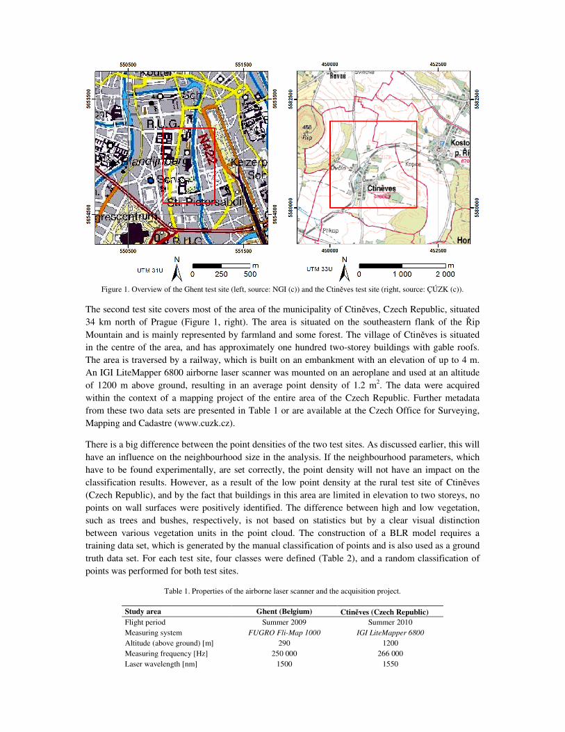
Figure 1. Overview of the Ghent test site (left, source: NGI (c)) and the Ctiněves test site (right, source: ÇÚZK (c)).

The second test site covers most of the area of the municipality of Ctiněves, Czech Republic, situated 34 km north of Prague (Figure 1, right). The area is situated on the southeastern flank of the Řip Mountain and is mainly represented by farmland and some forest. The village of Ctiněves is situated in the centre of the area, and has approximately one hundred two-storey buildings with gable roofs. The area is traversed by a railway, which is built on an embankment with an elevation of up to 4 m. An IGI LiteMapper 6800 airborne laser scanner was mounted on an aeroplane and used at an altitude of 1200 m above ground, resulting in an average point density of 1.2 m2. The data were acquired within the context of a mapping project of the entire area of the Czech Republic. Further metadata from these two data sets are presented in Table 1 or are available at the Czech Office for Surveying, Mapping and Cadastre (www.cuzk.cz).

There is a big difference between the point densities of the two test sites. As discussed earlier, this will have an influence on the neighbourhood size in the analysis. If the neighbourhood parameters, which have to be found experimentally, are set correctly, the point density will not have an impact on the classification results. However, as a result of the low point density at the rural test site of Ctiněves (Czech Republic), and by the fact that buildings in this area are limited in elevation to two storeys, no points on wall surfaces were positively identified. The difference between high and low vegetation, such as trees and bushes, respectively, is not based on statistics but by a clear visual distinction between various vegetation units in the point cloud. The construction of a BLR model requires a training data set, which is generated by the manual classification of points and is also used as a ground truth data set. For each test site, four classes were defined (Table 2), and a random classification of points was performed for both test sites.

Table 1. Properties of the airborne laser scanner and the acquisition project.

Study area Ghent (Belgium) Ctiněves (Czech Republic)

Flight period Summer 2009 Summer 2010 Measuring system FUGRO Fli-Map 1000 IGI LiteMapper 6800

Altitude (above ground) [m] 290 1200 Measuring frequency [Hz] 250 000 266 000 Laser wavelength [nm] 1500 1550

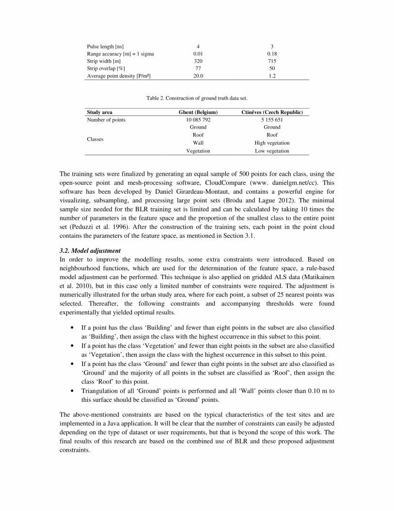
Pulse length [ns] 4 3 Range accuracy [m] = 1 sigma 0.01 0.18 Strip width [m] 320 715 Strip overlap [%] 77 50 Average point density [P/m²] 20.0 1.2

Table 2. Construction of ground truth data set.

Study area Ghent (Belgium) Ctiněves (Czech Republic)

Number of points 10 085 792 5 155 651

Classes

Ground Ground

Roof Roof

Wall High vegetation

Vegetation Low vegetation

The training sets were finalized by generating an equal sample of 500 points for each class, using the open-source point and mesh-processing software, CloudCompare (www. danielgm.net/cc). This software has been developed by Daniel Girardeau-Montaut, and contains a powerful engine for visualizing, subsampling, and processing large point sets (Brodu and Lague 2012). The minimal sample size needed for the BLR training set is limited and can be calculated by taking 10 times the number of parameters in the feature space and the proportion of the smallest class to the entire point set (Peduzzi et al. 1996). After the construction of the training sets, each point in the point cloud contains the parameters of the feature space, as mentioned in Section 3.1.

3.2. Model adjustment

In order to improve the modelling results, some extra constraints were introduced. Based on neighbourhood functions, which are used for the determination of the feature space, a rule-based model adjustment can be performed. This technique is also applied on gridded ALS data (Matikainen et al. 2010), but in this case only a limited number of constraints were required. The adjustment is numerically illustrated for the urban study area, where for each point, a subset of 25 nearest points was selected. Thereafter, the following constraints and accompanying thresholds were found experimentally that yielded optimal results.

• If a point has the class ‘Building’ and fewer than eight points in the subset are also classified as ‘Building’, then assign the class with the highest occurrence in this subset to this point.

• If a point has the class ‘Vegetation’ and fewer than eight points in the subset are also classified as ‘Vegetation’, then assign the class with the highest occurrence in this subset to this point.

• If a point has the class ‘Ground’ and fewer than eight points in the subset are also classified as ‘Ground’ and the majority of all points in the subset are classified as ‘Roof’, then assign the class ‘Roof’ to this point.

• Triangulation of all ‘Ground’ points is performed and all ‘Wall’ points closer than 0.10 m to this surface should be classified as ‘Ground’ points.

The above-mentioned constraints are based on the typical characteristics of the test sites and are implemented in a Java application. It will be clear that the number of constraints can easily be adjusted depending on the type of dataset or user requirements, but that is beyond the scope of this work. The final results of this research are based on the combined use of BLR and these proposed adjustment constraints.

4. Results

4.1. Multicollinearity within the feature space

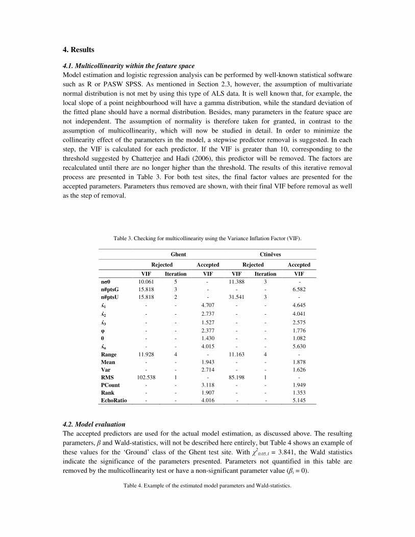
Model estimation and logistic regression analysis can be performed by well-known statistical software such as R or PASW SPSS. As mentioned in Section 2.3, however, the assumption of multivariate normal distribution is not met by using this type of ALS data. It is well known that, for example, the local slope of a point neighbourhood will have a gamma distribution, while the standard deviation of the fitted plane should have a normal distribution. Besides, many parameters in the feature space are not independent. The assumption of normality is therefore taken for granted, in contrast to the assumption of multicollinearity, which will now be studied in detail. In order to minimize the collinearity effect of the parameters in the model, a stepwise predictor removal is suggested. In each step, the VIF is calculated for each predictor. If the VIF is greater than 10, corresponding to the threshold suggested by Chatterjee and Hadi (2006), this predictor will be removed. The factors are recalculated until there are no longer higher than the threshold. The results of this iterative removal process are presented in Table 3. For both test sites, the final factor values are presented for the accepted parameters. Parameters thus removed are shown, with their final VIF before removal as well as the step of removal.

Table 3. Checking for multicollinearity using the Variance Inflation Factor (VIF).

Ghent Ctiněves

Rejected Accepted Rejected Accepted

VIF Iteration VIF VIF Iteration VIF

nσ0 10.061 5 - 11.388 3 - n#ptsG 15.818 3 - - - 6.582 n#ptsU 15.818 2 - 31.541 3 -

ʎ1 - - 4.707 - - 4.645

ʎ2 - - 2.737 - - 4.041

ʎ3 - - 1.527 - - 2.575

φ - - 2.377 - - 1.776 θ - - 1.430 - - 1.082

ʎn - - 4.015 - - 5.630

Range 11.928 4 - 11.163 4 - Mean - - 1.943 - - 1.878 Var - - 2.714 - - 1.626 RMS 102.538 1 - 85.198 1 - PCount - - 3.118 - - 1.949 Rank - - 1.907 - - 1.353 EchoRatio - - 4.016 - - 5.145

4.2. Model evaluation

The accepted predictors are used for the actual model estimation, as discussed above. The resulting parameters, β and Wald-statistics, will not be described here entirely, but Table 4 shows an example of these values for the ‘Ground’ class of the Ghent test site. With χ2

0.05,1 = 3.841, the Wald statistics indicate the significance of the parameters presented. Parameters not quantified in this table are removed by the multicollinearity test or have a non-significant parameter value (βi = 0).

Table 4. Example of the estimated model parameters and Wald-statistics.

ββββi Wald ββββi Wald

nσ0 - -

Range - -

n#ptsG - - Mean 0.663 29.085

n#ptsU

VAR -0.194 19.878

ʎ1 -4.924 36.083

RMS - -

ʎ2 - -

PCount 0.166 34.890

ʎ3 - - Rank -0.010 15.080

φ -6.683 119.468

EchoRatio 0.051 56.824

θ - -

Constant -7.595 70.957

ʎn 6.873 55.477

The overall model statistics allow the statistical acceptance of the models, as demonstrated in Table 5. With χ2

0.05,1 = 3.841, the likelihood ratios G2 are significant for all classes with a 95% level of

significance. The coefficients of determination, R2, suggest that a sufficient amount of variance is

explained by the model. However, the roof classifier of the Ghent study area and the low vegetation classifier of the Ctiněves study area have low R2 values. As explained below, visualization of these areas will clarify these low values.

Table 5. Evaluation of the significance of the entire model.

Ghent

Iteration G² Nagelkerke R²

Ground 8 972.075 0.699 Roof 6 1608.674 0.406 Vegetation 6 1132.240 0.634 Wall 8 1184.435 0.611

Ctiněves

Step G² Nagelkerke R²

Ground 9 759.717 0.778 Roof 9 1489.857 0.468 Low vegetation 6 2015.859 0.163 High vegetation 9 921.049 0.719

Table 6. Comparison between the errors of the BLR method and LASTools and MCC classification method.

Ghent Ctiněves

Class Algorithm Type I (%) Type II (%) Type I (%) Type II (%)

Ground

BLR 0.42 0.52 7.72 3.82

LASTOOLS 0.09 7.23 3.34 2.23

MCC 0.66 0.99 4.04 4.55

Unknown

class

BLR 3.22 1.72 7.33 5.25

LASTOOLS 1.62 4.72 3.03 6.48

Building BLR 3.91 2.39 2.01 6.41

LASTOOLS 5.26 1.07 6.04 0.54

Vegetation BLR 2.31 5.23 1.15 2.73

LASTOOLS 1.22 1.97 0.58 3.75

The errors in the final models are summarized in terms of both Type I errors (a point is incorrectly categorized as another class) and Type II (a class is incorrectly assigned to a point), as seen in Table 6. The same statistics are also presented for comparative filtering using LASTools and MCC. Both classifiers perform ground point and non-ground point filtering, respectively based on the local slope and curvature of a certain neighbourhood. After this filtering, LASTools also enables the classification of roofs and vegetation by the analysis of planarity or irregularity of non-ground points. By using LASTools, it is possible to automatically detect the classes ‘Ground’, ‘Roof’, ‘Vegetation’, and ‘Unknown’. Since MCC detects only ground points, the technique is not described for other classes. These two techniques are selected for comparison because of their avail- ability on the Internet and the fact that they can be used directly using stand-alone applications. In contrast to the classification method presented in this article, detectable classes are fixed for both techniques.

For comparison among algorithms, the detected classes based on BLR are translated to standard LAS classes. So ‘Walls’ in the urban area are set to ‘Unknown class’. Notwithstanding the fact that ‘Low vegetation’ is a standard LAS class, it is not explicitly implemented in the LASTools algorithm. ‘Building’ class in LAS is actually a classification of roof points of a point cloud, and therefore the wall points detected by the BLR technique do not fit in this class. This performance comparison with other techniques already indicates one of the main advantages of the newly developed point classification procedure, as it allows enlargement of or changing the range of classes that can potentially be detected. In general, the figures are in line with previously published comparisons of other classifiers (e.g. Chen et al. 2013).

The overall success of the classification method described is obvious for both the urban study area of Ghent and the rural area of Ctiněves. Although the results are not the same for the different classes, the ‘Ground’ classification of the urban area is very good. For all other classes, both the Type I and Type II error of BLR are lower than in the other classification algorithm. The ‘Building’ and ‘Vegetation’ classification of the rural area resulted in a better classified point cloud than the urban point cloud, taking into account both Type I and Type II errors. This classification error in the urban test site is mainly caused by the mixture of classes directly under the tree canopy. Type I error of ‘Ground’ and ‘Other’ classes of the rural area is relatively high. For the rural area point cloud, a manual classification was performed as ground truth for the quality analysis, based on a user interpretation of the relatively low-density point cloud. As a result, this data set is not free from human errors and this has an influence on quality assessment. This becomes clear with the comparison of BLR classification results to an ortho image, as discussed below.

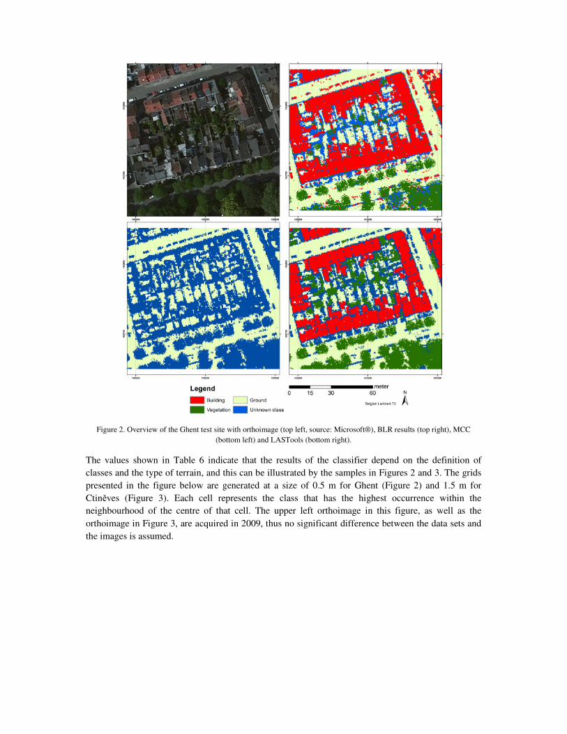
Figure 2. Overview of the Ghent test site with orthoimage (top left, source: Microsoft®), BLR results (top right), MCC (bottom left) and LASTools (bottom right).

The values shown in Table 6 indicate that the resultsclasses and the type of terrain, and this can be illustrated by the samples in Figures 2 and 3. The grids presented in the figure below are generated at a size of 0.5 m for Ghent (Figure 2) and 1.5 m for Ctiněves (Figure 3). Each cell represents the class that has the highest occurrence within the neighbourhood of the centre of that cell. The upper left orthoimage in this figure, as well as the orthoimage in Figure 3, are acquired in 2009, thus no significant dthe images is assumed.

Figure 2. Overview of the Ghent test site with orthoimage (top left, source: Microsoft®), BLR results (top right), MCC (bottom left) and LASTools (bottom right).

The values shown in Table 6 indicate that the results of the classifier depend on the definition of classes and the type of terrain, and this can be illustrated by the samples in Figures 2 and 3. The grids presented in the figure below are generated at a size of 0.5 m for Ghent (Figure 2) and 1.5 m for

ves (Figure 3). Each cell represents the class that has the highest occurrence within the neighbourhood of the centre of that cell. The upper left orthoimage in this figure, as well as the orthoimage in Figure 3, are acquired in 2009, thus no significant difference between the data sets and

Figure 2. Overview of the Ghent test site with orthoimage (top left, source: Microsoft®), BLR results (top right), MCC

of the classifier depend on the definition of classes and the type of terrain, and this can be illustrated by the samples in Figures 2 and 3. The grids presented in the figure below are generated at a size of 0.5 m for Ghent (Figure 2) and 1.5 m for

ves (Figure 3). Each cell represents the class that has the highest occurrence within the neighbourhood of the centre of that cell. The upper left orthoimage in this figure, as well as the

ifference between the data sets and

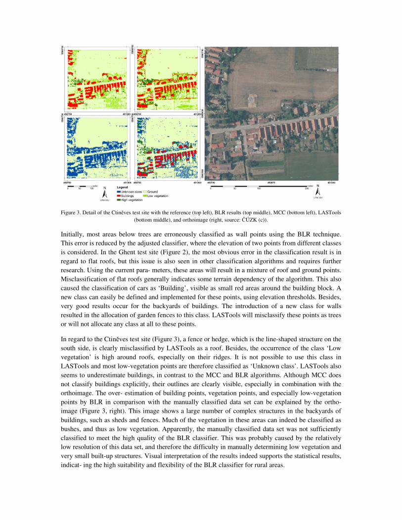
Figure 3. Detail of the Ctiněves test site with the reference (top left), BLR results (top middle), MCC (bottom left), LASTools (bottom middle), and orthoimage (right, source: ČÚZK (c)).

Initially, most areas below trees are erroneously classified as wall points using the BLR technique. This error is reduced by the adjusted classifier, where the elevation of two points from different classes is considered. In the Ghent test site (Figure 2), the most obvious error in the classification result is in regard to flat roofs, but this issue is also seen in other classification algorithms and requires further research. Using the current para- meters, these areas will result in a mixture of roof and ground points. Misclassification of flat roofs generally indicates some terrain dependency of the algorithm. This also caused the classification of cars as ‘Building’, visible as small red areas around the building block. A new class can easily be defined and implemented for these points, using elevation thresholds. Besides, very good results occur for the backyards of buildings. The introduction of a new class for walls resulted in the allocation of garden fences to this class. LASTools will misclassify these points as trees or will not allocate any class at all to these points.

In regard to the Ctiněves test site (Figure 3), a fence or hedge, which is the line-shaped structure on the south side, is clearly misclassified by LASTools as a roof. Besides, the occurrence of the class ‘Low vegetation’ is high around roofs, especially on their ridges. It is not possible to use this class in LASTools and most low-vegetation points are therefore classified as ‘Unknown class’. LASTools also seems to underestimate buildings, in contrast to the MCC and BLR algorithms. Although MCC does not classify buildings explicitly, their outlines are clearly visible, especially in combination with the orthoimage. The over- estimation of building points, vegetation points, and especially low-vegetation points by BLR in comparison with the manually classified data set can be explained by the ortho- image (Figure 3, right). This image shows a large number of complex structures in the backyards of buildings, such as sheds and fences. Much of the vegetation in these areas can indeed be classified as bushes, and thus as low vegetation. Apparently, the manually classified data set was not sufficiently classified to meet the high quality of the BLR classifier. This was probably caused by the relatively low resolution of this data set, and therefore the difficulty in manually determining low vegetation and very small built-up structures. Visual interpretation of the results indeed supports the statistical results, indicat- ing the high suitability and flexibility of the BLR classifier for rural areas.

4.3. Classification performance

Obviously, LASTools is targeted towards production workflows and has been optimized after its first release 10 years ago. The efficiency of the current version of the BLR-based prototype is estimated at half that of LASTools. The calculation of feature spaces and accompanying probabilities per point is reasonably computational intensive. In this con- text, the processing time increased quadratically for feature space determination and linearly for the probability calculation. However, it is possible to optimize the efficiency of the procedure by implementation of iterative classifiers, tiled processing, or point cloud indexing, etc. It must be emphasized that despite increased processing time, many conventional point classifiers are unable to take generic classes into account. For point cloud classification using regular classes (ground, roofs, and vegetation), conventional classifiers may be more suitable, but for more complex scenes, BLR-based classification is a reliable alternative for user-defined classes. It is also expected that subsequent reuse of the training sets for point cloud filtering of the same scene, or for the filtering of similar areas, would result in considerable time saving.

Supervised classification techniques are well known in regard to image based processing, where the construction of training sets is performed in 2D. The generation of training sets for BLR-based classification is facilitated by 3D software, minimizing the amount of noise in the sets. Moreover, the quality of the training sets can be assessed by evaluating the uniformity of the distributions of all parameters in the feature space. For the classification of very complex features, it can be assumed that an unsupervised point cloud classification can be used. In this case, a cluster analysis on the feature space could enable the automated classification of point clouds, without explicitly assigning semantics to the resulting classes.

5. Conclusion and further work

In this article, the use of BLR analysis for ALS point set classification is discussed. In contrast to current classification techniques, using one or a limited number of geometric criteria for the assignment of a point to a class, the proposed method makes use of a large feature space, the parameters of which are also based on the geometry of the neighbour- hood. Rather than constructing a threshold-based decision tree, the entire feature space is used for the generation of a series of logistic models for each class. These models calculate the probability that a point belongs to a certain class. Since a probability is assigned to each point for each class, the class assignment will be based on the highest probability. The method also enables model evaluation by statistical inference. Nevertheless, using the above classification technique, the use of BLR for ALS point set classification appears promising.

The procedure is explained by the classification of two different ALS data sets. The first is a dense point set of an urban area in the city of Ghent, Belgium. For this area, ground and non-ground filtering with a Type I error of 4% and an overall correctness of 95% was achieved. For the second test site, located around the rural village of Ctiněves (Czech Republic), a Type I error of 8% and an overall correctness of 96% were recorded. These values are in line with other state-of-the-art classification methods for ground point extraction. However, in contrast to most other classification methods, multiple classes can be extracted from an ALS point set.

The potential of the new classification procedure has been demonstrated for ALS data. In contrast to LASTools, the method does not require that the data be acquired from an airborne platform, and it can also be extended to Static Terrestrial Laser Scanning (STLS) and Mobile Terrestrial Laser Scanning (MTLS). Care needs to be taken with respect to the different properties of ALS on the one hand and STLS and MTLS on the other. For terrestrial scanning, variation in point density (caused by data

heterogeneity) and data holes (caused by shadows) must be taken into account. Furthermore, the feature space should not only contain parameters that are dependent of the elevation, such as local mean and standard deviation, but also parameters that take all dimensions into account, such as planimetric distribution descriptors or local eigenvalues. Besides, parameters related to the measured distance or intensity can be used for unprocessed STLS measurements, and colour information can be used for many MTLS point clouds.

The ability to generate a wide range of classes is the greatest strength of the proposed method. This user adaptability of the algorithm, dependent on the type of measurement area and the user’s experience, allows a very wide range of applications in the field of point classification supported by a thorough statistical basis for interpretation of the performance of the results. Moreover, not only can the BLR procedure itself be optimized, but also the model adjustment constraints can be fine-tuned depending on the application. If the training sets are defined correctly, the ratio of misclassified points will be around 5–12%. It should be mentioned that parameters other than those mentioned in this article could be taken into account. Besides, the results obtained appear very promising in regard to further improvement in the classification procedure (e.g. by either taking the neighbourhood of the class assignment into account or the use of a rough DTM for the calculation of a preparatory normalized elevation model).

Acknowledgements

The authors would like to express their gratitude to the city of Ghent and to the government of the Czech Republic for the airborne laser scanning data. The Czech data set was classified by Petr Hoffman. The Ludwig Boltzmann Institute for Archaeological Prospection and Virtual Archaeology is based on international cooperation of the Ludwig Boltzmann Gesellschaft (Austria), the University of Vienna (Austria), the Vienna University of Technology (Austria), the Austrian Central Institute for Meteorology and Geodynamics, the office of the provincial government of Lower Austria, Airborne Technologies GmbH (Austria), RGZM (Roman-Germanic Central Museum Mainz, Germany), RA (Swedish National Heritage Board), VISTA (Visual and Spatial Technology Centre, University of Birmingham, UK), and NIKU (Norwegian Institute for Cultural Heritage Research).

Funding

This study is part of the research project ‘3D CAD modelling of spatial architectural volumes, using terrestrial laser scanning and LiDAR’, supported by the Research Foundation Flanders (FWO, Belgium).

References

Baltsavias, E. 1999. "Airborne laser scanning: basic relations and formulas." Review of. ISPRS Journal of Photogrammetry and Remote Sensing 54 (2-3):199-214.

Bartels, M., and H. Wei. 2010. "Threshold-free object and ground point separation in LiDAR data." Review of. Pattern Recognition Letters 31 (10):1089-99.

Brenner, C. 2005. "Building reconstruction from images and laser scanning." Review of. International Journal of Applied Earth Observation and Geoinformation 6 (3-4):187-98.

Briese, C. 2010. "Extraction of digital terrain models." In Airborne and terrestrial laser scanning, edited by G. Vosselman and H Maas, 135-67. Dunbeath, UK: Whittles Publishing.

Briese, C., N. Pfeifer, and P. Dorninger. 2002. "Applications of the Robust Interpolation for DTM Determination." Review of. International Archives of Photogrammetry and Remote Sensing 34 (Part A):55-61.

Brodu, N., and D. Lague. 2012. "3D terrestrial LiDAR data classification of complex natural scenes using a multi-scale dimensionality criterion: applications in geomorphology." Review of. ISPRS Journal of Photogrammetry and Remote Sensing 68 (1):121-34.

Chatterjee, S., and B. Prince. 1991. "Analysis of collinear data." In Regression Diagnostics, 221-58. Hoboken, NJ, USA: John Wiley.

Chen, C., C. Li, W. Li, and H. Dai. 2013. "A multiresolution classification algorithm for filtering airborne LiDAR data." Review of. ISPRS Journal for Photogrammetry and Remote Sensing 82 (1):1-9.

Doneus, M., C. Briese, M. Fera, and M. Janner. 2008. "Archaeological prospection of forested areas using full-waveform airborne laser scanning." Review of. Journal of Archaeological Science 35 (4):882-93.

Dorninger, P., and N. Pfeifer. 2008. "A comprehensive automated 3D approach for building extraction, reconstruction and regularization from airborne laser scanning point clouds." Review of. Sensors 8 (11):7323-43.

Evans, J., and A. Hudak. 2007. "A multiscale curvature algorithm for classifying discrete return LiDAR in forested environments." Review of. IEEE Transactions on Geoscience and Remote Sensing 45 (4):1029-38.

Filin, S. 2002. "Surface clustering from airborne laser scanning data." Review of. International Archives of Photogrammetry and Remote Sensing and Spatial Information Sciences 34 (Part 3):119-24.

Filin, S., and N. Pfeifer. 2005. "Neighborhood systems for airborne laser data." Review of. Photogrammetric Engeneering and Remote Sensing 71 (6):743-55.

Flury, B. 1997. A first course in multivariate statistics. New York, NY, USA: Springer. Höfle, B., W. Mücke, M. Dutter, M. Rutzinger, and P. Dorninger. 2009. Detection of building regions

using airborne LiDAR: a new combination of raster and point cloud based GIS methods. Paper presented at the GI-Forum 2009 - International Conference on Applied Geoinformatics, Salzburg, Austria, July 7-10, 2009.

Hosmer, D., and S. Lemeshow. 2004. Applied logistic regression. Hoboken, NJ, USA.: John Wiley. Isenburg, Martin, and Jonathan Shewchuk. 2013. "LAStools." In, Converting, viewing and

compressing LIDAR data in LAS format. http://www.cs.unc.edu/~isenburg/lastools/. Kraus, K., and N. Pfeifer. 1998. "Determination of terrain models in wooded areas with airborne laser

scanner data." Review of. ISPRS Journal of Photogrammetry and Remote Sensing 53 (8):193-203.

Kutner, M., C. Nachtsheim, J. Neter, and W. Li. 2005. Applied linear statistical models. New York, NY, USA: McGray-Hill.

Li, Y. 2013. "Filtering airborne LiDAR data by in improved morphological method based on multi-gradient analysis." Review of. International Archives of Photogrammetry and Remote Sensing and Spatial Information Sciences 40 (1):191-4.

Mandlburger, G., J. Otepka, W. Karel, W. Wagner, and N. Pfeifer. 2009. "Orientation and processing of airborne laser scanning data (OPALS): concept and first results of a comprehensive ALS software." Review of. International Archives of Photogrammetry and Remote Sensing and Spatial Information Sciences 38 (Part 3):55-60.

Matikainen, L., J. Hyyppä, E. Ahokas, L. Markelin, and H. Kaartinen. 2010. "Automatic detection of buildings and changes in buildings for updating of maps." Review of. Remote Sensing 2 (5):1217-48.

Menard, S. 2010. Logistic regression: from introduction to advanced concepts and applications. Thousand Oaks, CA, USA: Sage Publications.

Meng, X., L. Wang, J. Silván-Gárdenas, and N. Currit. 2009. "A multi-directional ground filtering algorithm for airborne LiDAR." Review of. ISPRS Journal of Photogrammetry and Remote Sensing 64 (1):117-24.

Mongus, D., and B. Žalik. 2012. "Parameter-free ground filtering of LiDAR data for automatic DTM generation." Review of. ISPRS Journal of Photogrammetry and Remote Sensing 67 (1):1-12.

Nagelkerke, N. 1991. "A note on a general definition of the coefficient of determination." Review of. Biometrika 78 (3):691-2.

O’Brien, R. 2007. "A caution regarding rules of thumb for variance inflation factors." Review of. Quality and Quality 41 (5):673-90.

Otepka, J., G. Mandlburger, and W. Karel. 2012. "The OPALS data manager: efficient data manager for processing large airborne laser scanning projects." Review of. International Archives of Photogrammetry and Remote Sensing and Spatial Information Sciences 39 (Part 3):153-9.

Oude Elberink, S., and G. Vosselman. 2011. "Quality analysis on 3D building models reconstructed from airborne laser scanning data." Review of. ISPRS Journal of Photogrammetry and Remote Sensing 66 (2):157-65.

Peduzzi, P., J. Concato, E. Kemper, T. Holford, and A. Feinstein. 1996. "A simulation study of the number of events per variable in logistic regression analysis." Review of. Journal of Clinical Epidemiology 49 (12):1373-9.

Peng, C., K. Lee, and G. Ingersoll. 2002. "An introduction to logistic regression analysis and reporting." Review of. Journal of Educational Research 96 (1):3-14.

Pfeifer, N., and G. Mandlburger. 2008. "LiDAR data filtering and DTM generation." In Topographic laser ranging and scanning: principles and processing, edited by J. Shan and C. Toth, 307-33. Boca Raton, Fl, USA: CRC Press.

Podobnikar, T., and A. Vrecko. 2012. "Digital elevation model from the best results of different filtering of a LiDAR point cloud." Review of. Transactions in GIS 16 (5):603-17.

Sampath, A., and J. Shan. 2010. "Segmentation and reconstruction of polyhedral building roofs from aerial LiDAR point clouds." Review of. IEEE Transactions on Geoscience and Remote Sensing 48 (3):1554-67.

Sithole, G., and G. Vosselman. 2004. "Experimental comparison of filter algorithms for bare-Earth extraction from airborne laser scanning point clouds." Review of. ISPRS Journal of Photogrammetry and Remote Sensing 59 (1-2):85-101.

Stal, C., A. De Wulf, Ph. De Maeyer, R. Goossens, T. Nuttens, and F. Tack. 2012. Statistical comparison of urban 3D models from photo modeling and airborne laser scanning. Paper presented at the SGEM, Albena, Bulgaria.

Stal, C., F. Tack, P. De Maeyer, A. De Wulf, and R. Goossens. 2013. "Airborne photogrammetry and LiDAR for DSM extraction and 3D change detection over an urban area: a comparative study." Review of. International Journal of Remote Sensing 34 (4):1087-110.

Stine, R. 1995. "Graphical interpretation of variance inflation factors." Review of. The American Statistician 49 (1):53-6.

Wagner, W., A. Ullrich, V. Ducic, T. Melzer, and N. Studnicka. 2006. "Gaussian decomposition and calibration of a novel small-footprint full-waveform digitising airborne laser scanner." Review of. ISPRS Journal of Photogrammetry and Remote Sensing 60 (12):100-12.

Xu, S., S. Oude Elberink, and G. Vosselman. 2012. "Entities and features for classification of airborne laser scanning data in urban area." Review of. ISPRS Annals of the Photogrammetry, Remote Sensing and Spatial Information Sciences 1 (4):257-62.