click here full article patterns of predictability in

Patterns of predictability in hydrological threshold systems

E. Zehe,1 H. Elsenbeer,1 F. Lindenmaier,1 K. Schulz,2 and G. Bloschl3

Received 4 October 2006; revised 5 February 2007; accepted 14 March 2007; published 20 July 2007.

[1] Observations of hydrological response often exhibit considerable scatter that isdifficult to interpret. In this paper, we examine runoff production of 53 sprinklingexperiments on the water-repellent soils in the southern Alps of Switzerland; simulatedplot scale tracer transport in the macroporous soils at the Weiherbach site, Germany; andrunoff generation data from the 2.3-km2 Tannhausen catchment, Germany, that hascracking soils. The response at the three sites is highly dependent on the initial soilmoisture state as a result of the threshold dynamics of the systems. A simple statisticalmodel of threshold behavior is proposed to help interpret the scatter in the observations.Specifically, the model portrays how the inherent macrostate uncertainty of initial soilmoisture translates into the scatter of the observed system response. The statistical modelis then used to explore the asymptotic pattern of predictability when increasing the numberof observations, which is normally not possible in a field study. Although the physicaland chemical mechanisms of the processes at the three sites are different, the predictabilitypatterns are remarkably similar. Predictability is smallest when the system state is close tothe threshold and increases as the system state moves away from it. There is inherentuncertainty in the response data that is not measurement error but is related to theobservability of the initial conditions.

Citation: Zehe, E., H. Elsenbeer, F. Lindenmaier, K. Schulz, and G. Bloschl (2007), Patterns of predictability in hydrological

threshold systems, Water Resour. Res., 43, W07434, doi:10.1029/2006WR005589.

1. Introduction

[2] Understanding predictive model uncertainty (its quan-tification and its reduction) is a major concern in hydrolog-ical science [Sivapalan et al., 2003]. This includes anunderstanding of how the uncertainties of model parame-ters, model structure, and inputs affect the uncertainty of themodel predictions. However, as pointed out by Beven[1996, p. 260], one cannot expect process models to bemore accurate than the repeatability of nature herself. Henceit is similarly important to understand how well one mayrepeat observations of cause and effect. Repeatability ofexperiments or observations is a prerequisite to the predict-ability of that system. A system one hopes to predict withperfect accuracy needs to give exactly the same response ifan experiment is repeated under identical conditions, i.e.,when the forcings and the initial states of the repeated trialsare exactly the same. However, distributed hydrologicalmeasurements are never exhaustive and therefore uncertain.Their support, spacing, and extent scales tend to be incom-patible with the scale of state variables and processesin natural systems [Bloschl and Sivapalan, 1995]. Forinstance, the space-time pattern of soil moisture is usuallyestimated from a set of point observations, for example,using time domain reflectometry (TDR). Typically, thesemeasurements do not even suffice to fully characterize the

spatial probability distribution of soil moisture at the catch-ment scales [Deeks et al., 2004; Western et al., 2004]. Evenif the probability density function (pdf) were known, thedetailed spatial pattern will still elude full quantification.[3] Hydrological states and, in particular, their spatial

patterns are hence not fully observable and inherentlyuncertain [Rundle et al., 2006]. Because of this, one cannever repeat an observation under truly identical conditionsalbeit under apparently identical conditions. Observations ofhydrological system response, such as tracer transportdepths, residence times, and runoff volumes, often exhibitconsiderable scatter, even if the initial and boundary con-ditions are apparently identical [Lischeid et al., 2000; Zeheet al., 2005; Zehe and Bloschl, 2004]. This implies a lack ofrepeatability and hence poor predictability. Unobserved(and indeed unobservable) small-scale variability in thestates along with nonlinear system characteristics mayexplain this lack of repeatability [Pitman and Stouffer,2006; Rundle et al., 2006; Zehe and Bloschl, 2004]. If wewant to understand the limits to the accuracy of modelpredictions, we have to understand how inherent uncertain-ties of state observations limit the repeatability of observa-tions of the hydrological system response, especially in thepresence of strongly nonlinear behavior such as thresholdcontrolled dynamics.[4] Pitman and Stouffer [2006] define threshold behavior

as abrupt changes in system dynamics that occur at time-scale that are much smaller than the usual timescales of thesystem. Threshold behavior can hence be considered as anextreme type of nonlinear dynamics. Threshold-type non-linearities occur when state variables switch from zero tononzero values [Bloschl and Zehe, 2005] as is the case for

1Institute of Geoecology, University of Potsdam, Potsdam, Germany.2UFZ-Center for Environmental Research, Leipzig, Germany.3Institute of Hydraulic and Water Resources Engineering, Vienna

University of Technology, Vienna, Austria.

Copyright 2007 by the American Geophysical Union.0043-1397/07/2006WR005589$09.00

W07434

WATER RESOURCES RESEARCH, VOL. 43, W07434, doi:10.1029/2006WR005589, 2007ClickHere

for

FullArticle

1 of 12

http://dx.doi.org/10.1029/2006WR005589

water levels of overland flow, rainfall rates, or flow inmacropore systems [Vogel et al., 2005; Zehe and Fluhler,2001b]. Threshold behavior may be further enhanced byemerging and vanishing features as in the case of swellingand cracking soils [Navar et al., 2002; Lindenmaier et al.,2006] and hydrophobic soils [e.g., DeJonge et al., 1999;Doerr and Thomas, 2000], and during phase transitions.[5] Zehe and Bloschl [2004] drew from the concept of

macrostates and microstates of gases in statistical mechanics[Tolman, 1979] to characterize the observability of statevariables in environmental systems. The microstate is rep-resented by the values of the kinetic energy of each of theindividual molecules in a volume of gas which are neverobservable. The macrostate, in contrast, is defined as theaverage kinetic energy (or gas temperature) of the gasmolecules in that volume, and it is the macrostate that isobservable. A very large number of possible microstates areconsistent with the same macrostate. The term ‘‘identicalstate’’ of two volumes of gas can only refer to their macro-states, as the microstates cannot be observed and hencecannot be compared.[6] In analogy, the microstate of initial soil moisture can

be defined as the true spatial pattern of soil moisture of,say, a field plot. Clearly, this microstate is not observableas there will always be fine-scale detail that cannot beresolved by the measurements. The macrostate can, forexample, be defined as the first two statistical moments,the variogram and the probability density function ofsoil moisture, as these are the variables that are observablein a typical field study. An infinite number of possible soilmoisture patterns (i.e., microstates) will be consistent withthe same observed macrostate. This will introduce uncer-tainty that will propagate through the system and causeuncertainty in the system response such as streamflow andinfiltration patterns.[7] Zehe and Bloschl [2004] conducted numerical simu-

lations to illustrate the effect of lack of knowledge of themicrostate on hydrologic response in the presence ofthreshold behavior. They found that, under apparentlyidentical conditions, repeated trials produced uncertaintyin system response of more than 100% of the averageresponse. So far, it has, however, been unclear whetherthese effects are consistent with the observed scatter ofhydrological field experiments and whether they apply toother threshold processes.[8] The objective of this paper is to contribute to a better

understanding of the repeatability of experiments and hencethe scatter of observed hydrological response by analyzingthe transformation of the inherent uncertainties of observedstates into uncertainties in hydrological response. We willexamine the transformation for three different processeswith threshold behavior at the plot and catchment scales.[9] This paper goes beyond that of Zehe and Bloschl

[2004] in a number of ways. First, we use field data fromthree case studies to examine three different processes thatinvolve threshold behavior, whereas Zehe and Bloschl [2004]used simulations for a single process (matrix/macroporeflow transitions). Second, we propose a statistical modelthat helps interpret field observations for a limited numberof trials relative to a hypothetical ensemble of an infinitenumber of observations.

[10] This paper is organized as follows. Section 2 reviewsthe three threshold processes for three field experiments andgives details on the field data. Section 3 presents thestatistical model and the methods to quantify the repeatabil-ity and hence predictability of the response. Section 4 givesthe results, which are discussed in section 5.

2. Threshold Processes, Study Sites, and Data

2.1. Plot Scale Runoff Generation in a Water-RepellentSoilscape

2.1.1. Water Repellency and Runoff Generation[11] The first process examined is runoff generation on

water-repellent soils. Water repellency was reported as earlyas 1910 by Schreiner and Shorey [1910] for soils inCalifornia that could be wetted neither by infiltration norby the rise of groundwater tables. Water repellency of soilsis related to degraded organic matter [Krammes andDeBano, 1965] and sometimes to forest fires [de Banoand Rice, 1973]. Water repellency is often associated withsandy soils and occasionally with clay soils. The maincontrols are the type of organic matter, the occurrence ofthe dry season, and the soil moisture [DeJonge et al., 1999].de Bano and Rice [1973] suggested that water repellencyoccurs after soil moisture drops below a certain threshold.Bond [1964] emphasized the role of organic matter coatingson coarse grains, whose hydrophobicity forces water to actas a nonwetting fluid that tries to minimize the interface tothe water-repellent environment. The most important con-cepts of quantifying the degree of hydrophobicity/waterrepellency are the ‘‘Water Drop Penetration Time’’ [Leteyet al., 2000], which is the time it takes for a water droplet toinfiltrate into the soil, and the ‘‘Molarity of AqueousEthanol Droplets’’ [King, 1981], which is the concentrationof an ethanol/water mix that infiltrates within 10 s into thesoil sample. The higher the molarity of the ethanol/watermix, the higher will be the degree of water repellency. Arecent bibliography on water repellency [Dekker et al.,2005] highlights the global occurrence of this phenomenon.Although its effects on runoff generation have been studiedglobally since the 1960s [e.g., Krammes and DeBano, 1965;Burch et al., 1989; Keizer et al., 2005], the role ofantecedent soil moisture over a range of scales has receivedmuch less attention [e.g., Doerr and Thomas, 2000; Doerret al., 2003].2.1.2. Sprinkling Experiments in the Southern SwissAlps[12] To shed light on the control of antecedent soil

moisture on surface runoff generation in a landscape withhydrophobic soils, we performed sprinkling experiments ina landscape prone to occasional droughts and wildfires. Theresearch area is located in southern Switzerland at 46�300N,9�010E at an elevation of about 720 m. Aspects range fromS to SW and slopes range from 20� and 37�. The area iscovered by mixed deciduous forest (Castanea sativa, Fagussilvatica, Quercus sp.). The dominant soil type is DystricCambisol [International Society of Soil Sciences/Interna-tional Soil Reference and Information Centre/Food andAgriculture Organization (ISSS-ISRIC-FAO), 1998]. Meanannual precipitation is 1800 mm, with a pronounced dryseason between December and March.

2 of 12

W07434 ZEHE ET AL.: PATTERNS OF PREDICTABILITY IN HYDROLOGICAL THRESHOLD SYSTEMS W07434

[13] Fifty-three sprinkling experiments were performedusing an automated sprinkling device [Ritschard, 2000]. Weapplied artificial rainfall with an intensity of 50 mm/h,which occurs with a return interval of 5 years. Each ofthe 53 test plots was 1 m2 in size. Figure 1 shows a typicalfield plot. To study the effect of dry periods, we covered theplots for a period ranging from 10 to 100 days. Runoff fromthe plots was measured manually, and initial soil moisturewas measured at two points in each plot using time domainreflectometry. Water repellency was estimated before eachsprinkling experiment by determining the water drop pen-etration time and by performing the molarity-of-ethanol-droplet test on air-dried soil samples [Letey et al., 2000].According to King’s [1981] classification, all plots with theexception of one were extremely hydrophobic at the onsetof the sprinkling experiments. Figure 2 shows examples ofobserved runoff at the field plot shown in Figure 1 for wetand dry antecedent soil moisture conditions (0.30 and0.07 m3 m�3, respectively). Because of the high saturatedhydraulic conductivities of about 5 � 10�5 m/s, a large partof the water infiltrates when the soil is wet. In contrast,when the soil is dry, surface runoff triples as a result ofwater repellency.

2.2. Plot Scale Tracer Transport in MacroporousHeterogeneous Soils

2.2.1. Preferential Flow and Solute Transport[14] The second process we examined is plot scale

transport in heterogeneous soils. When dealing with con-tamination of shallow groundwater, preferential flow oftenis a key process [Stamm et al., 1998; Flury, 1996; Zehe andFluhler, 2001a]. Typical transport distances of preferentialflow events in macroporous soils are on the order of 50–100 cm [Flury, 1996]. The main control on the occurrenceof preferential flow in macropores is the presence ofinterconnected preferential pathways that link the soilsurface and the subsoil [Vogel et al., 2005; Zehe andFluhler, 2001b]. Other important controls are soil moistureand rainfall magnitude as found, for example, by the dyetracer experiments in the Weiherbach catchment [Zehe andFluhler, 2001b].2.2.2. Simulated Replicates of Plot Scale TransportExperiments in a Macroporous Soil[15] In this example, we use results from Monte Carlo

simulations that are based on plot scale tracer experimentson a 1-m2 field site in a highly macroporous Colluvisol

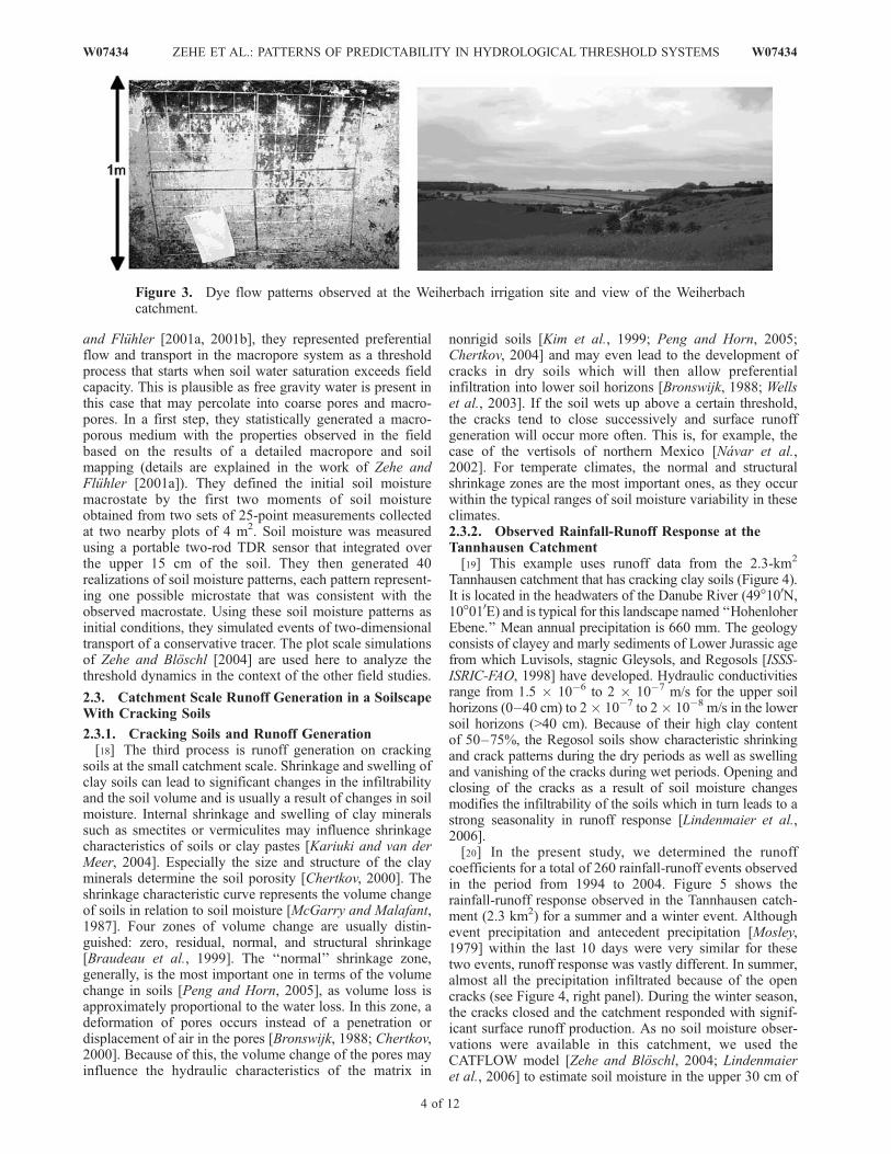
[ISSS-ISRIC-FAO, 1998]. The study site is located in therural Weiherbach valley at 49�010N, 9�000E which is atypical catchment for this landscape named ‘‘Kraichgau.’’Preferential flow events at this study site were observedseveral times: Tracer transport depths observed during plotscale tracer experiments (Figure 3) were much larger thanpredicted when assuming that matrix flow was the onlyrelevant process [Zehe and Bloschl, 2004]. Furthermore,observed tracer breakthrough into tile drains located at 1.2 mbelow surface was faster by 2 to 3 orders of magnitude thansimulations based on matrix flow and transport assumptions[Zehe and Fluhler, 2001a].[16] Geologically, the Weiherbach valley consists of

Keuper and Loess layers of up to 15-m thickness. Theclimate in the Weiherbach valley is humid with an averageannual precipitation of 750–800 mm, average annual runoffof 150 mm, and annual potential evapotranspiration of775 mm. Most of the Weiherbach hillslopes exhibit a typicalloess catena with the moist but drained Colluvisols at thehill foot and drier Calcaric Regosols [ISSS-ISRIC-FAO,1998] at the top and midslope sector. Interconnected prefe-rential pathways are apparent in the Colluvisol and are aresult of earthworm activities (anecic earthworms such asLumbricus terrestris).[17] Zehe and Bloschl [2004] simulated repeated trials of

the transport experiments by the physically based CAT-FLOW model. The model was extensively tested againstfield data of that site. On the basis of the findings of Zehe

Figure 1. Sprinkling setup in the southern Swiss Alps.

Figure 2. Surface runoff in response to irrigation of theplot shown in Figure 1 with wet (7 May) and dry (7 July)antecedent soil moisture conditions.

W07434 ZEHE ET AL.: PATTERNS OF PREDICTABILITY IN HYDROLOGICAL THRESHOLD SYSTEMS

3 of 12

W07434

and Fluhler [2001a, 2001b], they represented preferentialflow and transport in the macropore system as a thresholdprocess that starts when soil water saturation exceeds fieldcapacity. This is plausible as free gravity water is present inthis case that may percolate into coarse pores and macro-pores. In a first step, they statistically generated a macro-porous medium with the properties observed in the fieldbased on the results of a detailed macropore and soilmapping (details are explained in the work of Zehe andFluhler [2001a]). They defined the initial soil moisturemacrostate by the first two moments of soil moistureobtained from two sets of 25-point measurements collectedat two nearby plots of 4 m2. Soil moisture was measuredusing a portable two-rod TDR sensor that integrated overthe upper 15 cm of the soil. They then generated 40realizations of soil moisture patterns, each pattern represent-ing one possible microstate that was consistent with theobserved macrostate. Using these soil moisture patterns asinitial conditions, they simulated events of two-dimensionaltransport of a conservative tracer. The plot scale simulationsof Zehe and Bloschl [2004] are used here to analyze thethreshold dynamics in the context of the other field studies.

2.3. Catchment Scale Runoff Generation in a SoilscapeWith Cracking Soils

2.3.1. Cracking Soils and Runoff Generation[18] The third process is runoff generation on cracking

soils at the small catchment scale. Shrinkage and swelling ofclay soils can lead to significant changes in the infiltrabilityand the soil volume and is usually a result of changes in soilmoisture. Internal shrinkage and swelling of clay mineralssuch as smectites or vermiculites may influence shrinkagecharacteristics of soils or clay pastes [Kariuki and van derMeer, 2004]. Especially the size and structure of the clayminerals determine the soil porosity [Chertkov, 2000]. Theshrinkage characteristic curve represents the volume changeof soils in relation to soil moisture [McGarry and Malafant,1987]. Four zones of volume change are usually distin-guished: zero, residual, normal, and structural shrinkage[Braudeau et al., 1999]. The ‘‘normal’’ shrinkage zone,generally, is the most important one in terms of the volumechange in soils [Peng and Horn, 2005], as volume loss isapproximately proportional to the water loss. In this zone, adeformation of pores occurs instead of a penetration ordisplacement of air in the pores [Bronswijk, 1988; Chertkov,2000]. Because of this, the volume change of the pores mayinfluence the hydraulic characteristics of the matrix in

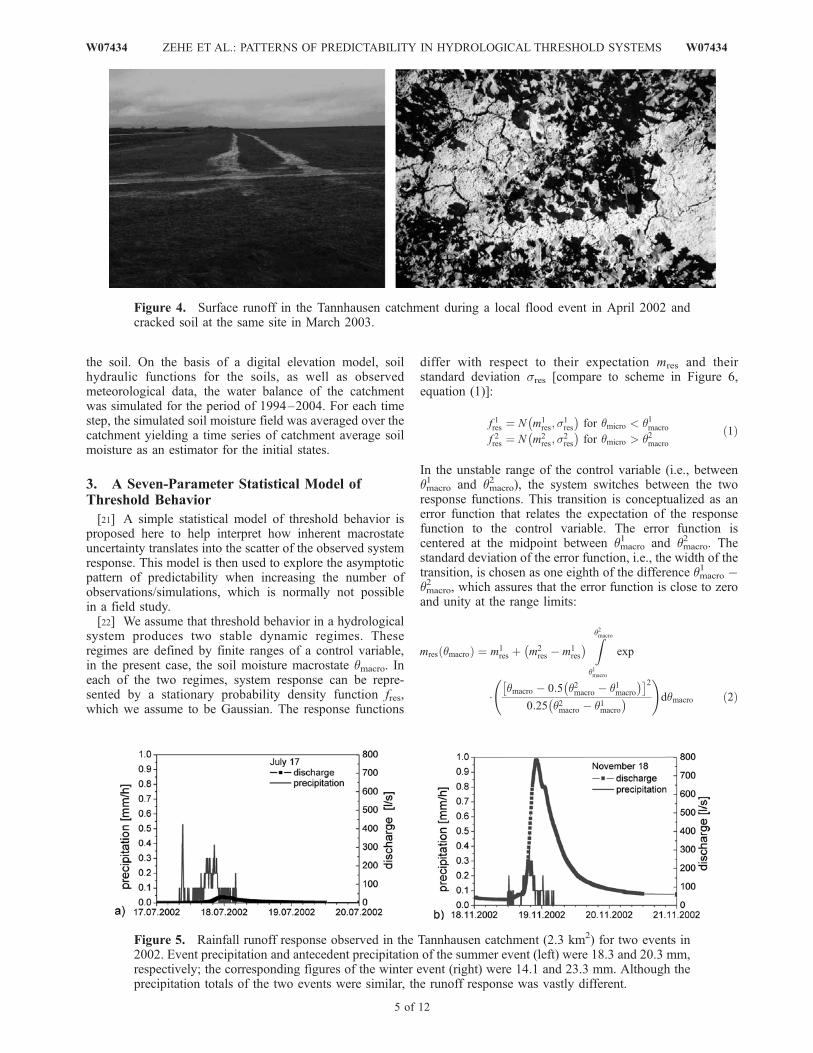
nonrigid soils [Kim et al., 1999; Peng and Horn, 2005;Chertkov, 2004] and may even lead to the development ofcracks in dry soils which will then allow preferentialinfiltration into lower soil horizons [Bronswijk, 1988; Wellset al., 2003]. If the soil wets up above a certain threshold,the cracks tend to close successively and surface runoffgeneration will occur more often. This is, for example, thecase of the vertisols of northern Mexico [Navar et al.,2002]. For temperate climates, the normal and structuralshrinkage zones are the most important ones, as they occurwithin the typical ranges of soil moisture variability in theseclimates.2.3.2. Observed Rainfall-Runoff Response at theTannhausen Catchment[19] This example uses runoff data from the 2.3-km2

Tannhausen catchment that has cracking clay soils (Figure 4).It is located in the headwaters of the Danube River (49�100N,10�010E) and is typical for this landscape named ‘‘HohenloherEbene.’’ Mean annual precipitation is 660 mm. The geologyconsists of clayey and marly sediments of Lower Jurassic agefrom which Luvisols, stagnic Gleysols, and Regosols [ISSS-ISRIC-FAO, 1998] have developed. Hydraulic conductivitiesrange from 1.5 � 10�6 to 2 � 10�7 m/s for the upper soilhorizons (0–40 cm) to 2� 10�7 to 2� 10�8 m/s in the lowersoil horizons (>40 cm). Because of their high clay contentof 50–75%, the Regosol soils show characteristic shrinkingand crack patterns during the dry periods as well as swellingand vanishing of the cracks during wet periods. Opening andclosing of the cracks as a result of soil moisture changesmodifies the infiltrability of the soils which in turn leads to astrong seasonality in runoff response [Lindenmaier et al.,2006].[20] In the present study, we determined the runoff

coefficients for a total of 260 rainfall-runoff events observedin the period from 1994 to 2004. Figure 5 shows therainfall-runoff response observed in the Tannhausen catch-ment (2.3 km2) for a summer and a winter event. Althoughevent precipitation and antecedent precipitation [Mosley,1979] within the last 10 days were very similar for thesetwo events, runoff response was vastly different. In summer,almost all the precipitation infiltrated because of the opencracks (see Figure 4, right panel). During the winter season,the cracks closed and the catchment responded with signif-icant surface runoff production. As no soil moisture obser-vations were available in this catchment, we used theCATFLOW model [Zehe and Bloschl, 2004; Lindenmaieret al., 2006] to estimate soil moisture in the upper 30 cm of

Figure 3. Dye flow patterns observed at the Weiherbach irrigation site and view of the Weiherbachcatchment.

4 of 12


the soil. On the basis of a digital elevation model, soilhydraulic functions for the soils, as well as observedmeteorological data, the water balance of the catchmentwas simulated for the period of 1994–2004. For each timestep, the simulated soil moisture field was averaged over thecatchment yielding a time series of catchment average soilmoisture as an estimator for the initial states.

3. A Seven-Parameter Statistical Model ofThreshold Behavior

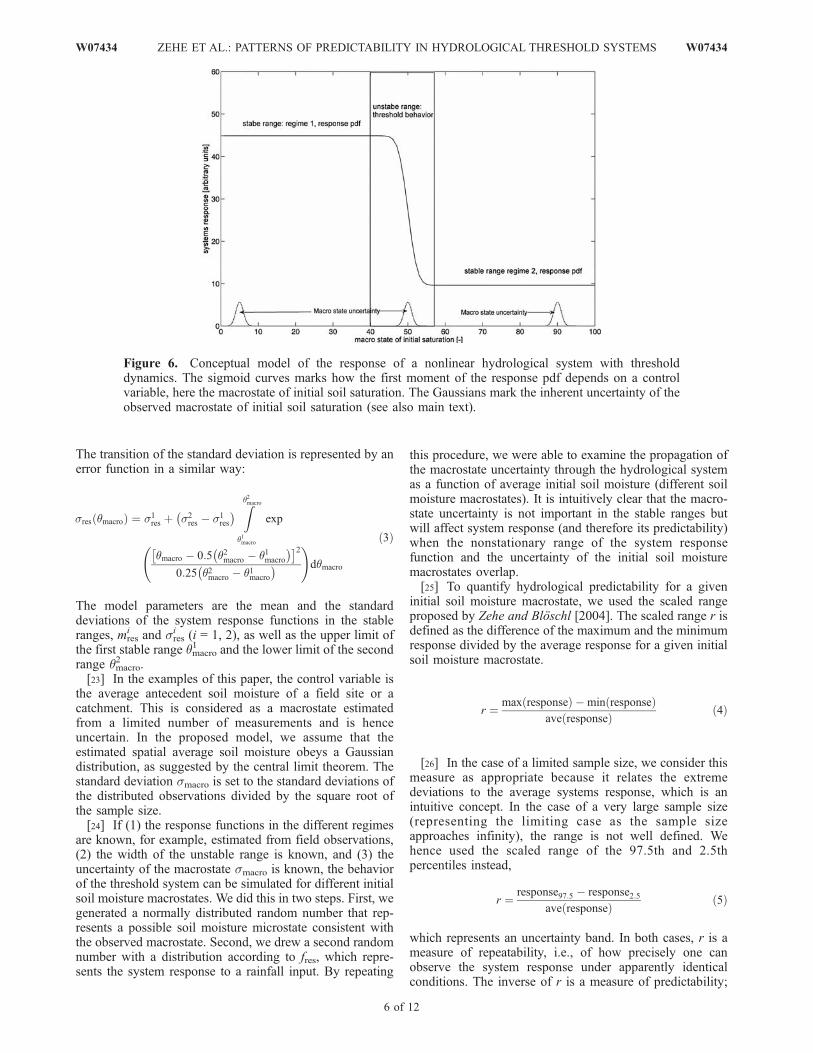
[21] A simple statistical model of threshold behavior isproposed here to help interpret how inherent macrostateuncertainty translates into the scatter of the observed systemresponse. This model is then used to explore the asymptoticpattern of predictability when increasing the number ofobservations/simulations, which is normally not possiblein a field study.[22] We assume that threshold behavior in a hydrological

system produces two stable dynamic regimes. Theseregimes are defined by finite ranges of a control variable,in the present case, the soil moisture macrostate qmacro. Ineach of the two regimes, system response can be repre-sented by a stationary probability density function fres,which we assume to be Gaussian. The response functions

differ with respect to their expectation mres and theirstandard deviation sres [compare to scheme in Figure 6,equation (1)]:

f 1res ¼ N m1res;s

1res

� �for qmicro < q1macro

f 2res ¼ N m2res;s

2res

� �for qmicro > q2macro

ð1Þ

In the unstable range of the control variable (i.e., betweenqmacro1 and qmacro

2 ), the system switches between the tworesponse functions. This transition is conceptualized as anerror function that relates the expectation of the responsefunction to the control variable. The error function iscentered at the midpoint between qmacro

1 and qmacro2 . The

standard deviation of the error function, i.e., the width of thetransition, is chosen as one eighth of the difference qmacro

1 �qmacro2 , which assures that the error function is close to zeroand unity at the range limits:

mres qmacroð Þ ¼ m1res þ m2

res � m1res

� � Zq2macro

q1macro

exp

��macro � 0:5 �2macro � �1macro

� �� 20:25 �2macro � �1macro

� � !

d�macro

ð2Þ

Figure 4. Surface runoff in the Tannhausen catchment during a local flood event in April 2002 andcracked soil at the same site in March 2003.

Figure 5. Rainfall runoff response observed in the Tannhausen catchment (2.3 km2) for two events in2002. Event precipitation and antecedent precipitation of the summer event (left) were 18.3 and 20.3 mm,respectively; the corresponding figures of the winter event (right) were 14.1 and 23.3 mm. Although theprecipitation totals of the two events were similar, the runoff response was vastly different.

ð2Þ


5 of 12

W07434

The transition of the standard deviation is represented by anerror function in a similar way:

sres qmacroð Þ ¼ s1res þ s2

res � s1res

� � Zq2macro

q1macro

exp

�macro � 0:5 �2macro � �1macro

� �� 20:25 �2macro � �1macro

� � !

d�macro

ð3Þ

The model parameters are the mean and the standarddeviations of the system response functions in the stableranges, mres

i and sresi (i = 1, 2), as well as the upper limit of

the first stable range qmacro1 and the lower limit of the second

range qmacro2 .

[23] In the examples of this paper, the control variable isthe average antecedent soil moisture of a field site or acatchment. This is considered as a macrostate estimatedfrom a limited number of measurements and is henceuncertain. In the proposed model, we assume that theestimated spatial average soil moisture obeys a Gaussiandistribution, as suggested by the central limit theorem. Thestandard deviation smacro is set to the standard deviations ofthe distributed observations divided by the square root ofthe sample size.[24] If (1) the response functions in the different regimes

are known, for example, estimated from field observations,(2) the width of the unstable range is known, and (3) theuncertainty of the macrostate smacro is known, the behaviorof the threshold system can be simulated for different initialsoil moisture macrostates. We did this in two steps. First, wegenerated a normally distributed random number that rep-resents a possible soil moisture microstate consistent withthe observed macrostate. Second, we drew a second randomnumber with a distribution according to fres, which repre-sents the system response to a rainfall input. By repeating

this procedure, we were able to examine the propagation ofthe macrostate uncertainty through the hydrological systemas a function of average initial soil moisture (different soilmoisture macrostates). It is intuitively clear that the macro-state uncertainty is not important in the stable ranges butwill affect system response (and therefore its predictability)when the nonstationary range of the system responsefunction and the uncertainty of the initial soil moisturemacrostates overlap.[25] To quantify hydrological predictability for a given

initial soil moisture macrostate, we used the scaled rangeproposed by Zehe and Bloschl [2004]. The scaled range r isdefined as the difference of the maximum and the minimumresponse divided by the average response for a given initialsoil moisture macrostate.

r ¼ maxðresponseÞ �minðresponseÞaveðresponseÞ ð4Þ

[26] In the case of a limited sample size, we consider thismeasure as appropriate because it relates the extremedeviations to the average systems response, which is anintuitive concept. In the case of a very large sample size(representing the limiting case as the sample sizeapproaches infinity), the range is not well defined. Wehence used the scaled range of the 97.5th and 2.5thpercentiles instead,

r ¼ response97:5 � response2:5aveðresponseÞ ð5Þ

which represents an uncertainty band. In both cases, r is ameasure of repeatability, i.e., of how precisely one canobserve the system response under apparently identicalconditions. The inverse of r is a measure of predictability;

Figure 6. Conceptual model of the response of a nonlinear hydrological system with thresholddynamics. The sigmoid curves marks how the first moment of the response pdf depends on a controlvariable, here the macrostate of initial soil saturation. The Gaussians mark the inherent uncertainty of theobserved macrostate of initial soil saturation (see also main text).

6 of 12


for example, small values of the range r indicate large (orfavorable) predictability.

4. Results

4.1. Plot Scale Runoff Generation in a Water-RepellentSoilscape

[27] Figure 7 (upper left panel) presents the total runoffvolumes (expressed as runoff depths) observed at the 53field sites in the southern Swiss Alps plotted against averageinitial soil moisture. Two stable regimes are apparent: runoffresponse with an average of 45 mm for initial soil moistureless than 0.11 m3 m�3, and a much weaker runoff responsein average of 9.5 mm for soil moisture greater than 0.21 m3

m�3. The difference between the average runoff valuesobserved in the two regimes is significant at a level of95%. In the unstable range between 0.11 and 0.21 m3 m�3

initial soil moisture, the runoff response exhibits a muchlarger variability than in each of the stable ranges. Fromthese data, we calculated the scaled range as a function ofaverage initial soil moisture [equation (4)]. After severaltests, we chose a width of 0.05 m3 m�3 for the soil moistureclasses, which is sufficiently fine to detect the uncertaintypeak and sufficiently coarse to give robust estimates of therange for this data set. The resulting scaled ranges peak inthe class centered at 0.225 m3 m�3 initial soil moisture(Figure 7, upper right panel). A peak value of 1.5 meansthat the total range of the runoff depths in this class is 150%

of the average response. Clearly, this would be consideredpoor repeatability and therefore poor predictability.[28] In a second step, we obtained the parameters of the

statistical model by estimating the mean and standarddeviations of the observed runoff depths in the two stableranges (Table 1). The uncertainty of the initial soil moisturemacrostate was set to the measurement error of the timedomain reflectometry device with a standard deviation ofsmacro = 0.02 m3 m�3. We then used the statistical model tosimulate runoff response of the sprinkling experiments andvaried the macrostate of average initial soil moisture. Thenumber of simulated experiments in each soil moisture classwas equal to the number of sprinkling experiments in thatclass. As can be seen from Figure 7 (left panels), thesimulated pattern of the runoff volumes is very similar tothe observed pattern. Also, the patterns of the scaled rangesof the simulations are quite similar to those of the observa-tions, although the peaks do not exactly coincide (Figure 7,right panels). For this relatively low number of trials at eachmacrostate, the pattern of the scaled range does not fullyreflect the patterns of the underlying statistical model.

4.2. Plot Scale Tracer Transport in MacroporousHeterogeneous Soils

[29] Figure 8 shows the simulated transport depths oneday after tracer application plotted against the averageinitial soil moisture (upper left panel). There are, again,two stable regimes for initial soil moisture, either smaller

Figure 7. Event surface runoff depths observed during the plot scale sprinkling experiments in thesouthern Swiss Alps plotted against average initial soil moisture macrostate, ism (upper left panel).Scaled ranges of the observed runoff depths plotted against soil moisture macrostate, ism (upper rightpanel). Lower panels show the corresponding graphs simulated by the statistical model.


7 of 12

W07434

than 0.15 m3 m�3 or larger than 0.25 m3 m�3. In these tworanges, the macrostate uncertainty translates into a smallscatter of the average tracer transport depths. Transportdynamics is stable with an expected transport depth of 0.04and 0.12 m, respectively, for the two regimes. In theunstable range between 0.15 and 0.25 m3 m�3, macrostateuncertainty is amplified and the average transport depthsfill the entire range between the two stable regimes. Thescaled ranges (Figure 8, upper right panel) peak at anaverage initial soil moisture of 0.18 m3 m�3 with a value of1.2. The maximum uncertainty of the transport depth ishence 120% of the average value.[30] The statistical model was, again, used to mimic the

behavior of the threshold system. The parameters wereestimated from the simulated output with the full dynamic

model and are given in Table 1. The uncertainty of the soilmoisture macrostate was estimated from the field data as0.02 m3 m�3. By generating 40 realizations for a givenaverage initial soil moisture, we obtained the scatterplot ofaverage transport depths and the scaled ranges (Figure 8,bottom panels). They are very similar to those of the fulldynamic model, although the statistical model is muchsimpler. The similarity in the patterns suggests that thestatistical model can indeed be used to help interpret thescatter in hydrological response measurements in case ofthreshold behavior.

4.3. Catchment Scale Runoff Generation in a SoilscapeWith Cracking Soils

[31] Figure 9 (upper left panel) presents the runoffcoefficients observed in the Tannhausen catchment plotted

Figure 8. Transport depths of the tracer center of mass of the simulated replicates at the Weiherbach siteplotted against average initial soil moisture macrostate, ism (upper left panel, circles). For comparison,the crosses show the transport depths for a similar soil but without macropores. Scaled ranges of thetransport depths plotted against soil moisture macrostate, ism (upper right panel). Lower panels show thecorresponding graphs simulated by the statistical model.

Table 1. Parameters of the Statistical Model for the Three Process Examples: Average Response Values and Standard Deviations of the

Two Regimes [mresi and sres

i (i = 1.2)], and Lower and Upper Limit of the Transition Region (qmacro1 ,qmacro

2 )a

Example mres1 sres

1 mres2 sres

2 qmacro1 , m3 m�3 qmacro

2 , m3 m�3 smacro, m3 m�3

S Alps 44.5 mm 9.6 mm 13.7 mm 4.6 mm 0.11 0.21 0.02Weiherbach 0.04 m 0.12 m 0.01 m 0.01 m 0.15 0.25 0.02Tannhausen 0.06 0.66 0.02 0.20 0.29 0.35 0.02

aThe macrostate uncertainty in terms of its standard deviation smacro is also shown. System response for the southern Swiss Alps example is observedevent runoff depth; for the Weiherbach example, it is average simulated tracer transport depth, and for the Tannhausen example, it is the observed eventrunoff coefficient.

8 of 12


against the average initial soil moisture. Similar to theother process examples, there are two stable ranges ofsystem response: weak runoff response with an averagerunoff coefficient of 0.06 for soil moisture less than0.29 m3 m�3, and significant runoff response with anaverage runoff coefficient of 0.66 for average monthly soilmoisture of more than 0.35 m3 m�3. Clearly, in the drierregime, the soil cracks are open, so most of the waterinfiltrates and does not produce surface runoff. In contrast,in the wet regime, the cracks are closed, so the contributionof rainfall to runoff is much larger. In the unstable rangebetween 0.29 and 0.35 m3 m�3, the scatter is large. Thescaled range of the observed runoff coefficients peaks at0.32 m3 m�3 average soil moisture with a maximum ofalmost 4. This means that total uncertainty in the runoffcoefficient is almost 400% of its average.[32] The parameters of the statistical model were obtained

in a similar way as in the other examples. The macrostateuncertainty was estimated as 0.02 m3 m�3 (Table 1) usingthe standard deviation within the model grid according toZehe and Bloschl [2004]. The simulation results are shownin the bottom panels of Figure 9. Again, the patterns arevery similar to those obtained from the measurements,although the model yields a lower peak for the scaled rangeand therefore a better repeatability than that suggested bythe data.[33] It is interesting that the patterns of runoff generation

on water-repellent soils (Figure 7) are similar to those ofplot scale transport in macroporous soils (Figure 8) andsimilar to the response patterns of the cracking soils(Figure 9). More specifically, in all cases, the repeatability

of the observations is poorest in the vicinity of the threshold,which points to a more generic pattern of predictability ofhydrologic response in the presence of threshold processes.

4.4. Asymptotic Simulations of the Statistical Model

[34] As the conceptual model of threshold behavior is of astatistical nature, it is clear that, for a small number of trials,the simulated system response and the scaled ranges willstrongly depend on the realization and exhibit a certainamount of randomness. This resembles the situation withfield data that are inherently difficult to interpret, as thenumber of trials will always be limited. The statisticalmodel proposed here can be used to shed light on the roleof the number of trials in observed system response.Specifically, we used the model to examine the asymptoticbehavior, i.e., the hypothetical case of having an infinitenumber of trials available for the same site. The model wasused to simulate system response with the parameters listedin Table 1, but the number of realizations was set to 10,000for each initial soil moisture state to obtain the results for theasymptotic behavior.[35] Figure 10 shows the results of this exercise. The

upper panels present the results for plot scale runoffgeneration on the water-repellent soils in the southern SwissAlps, the center panels those for plot scale tracer transport inthe macroporous soils at the Weiherbach site, and the lowerpanels those for runoff generation on the cracking soils inthe Tannhausen catchment. The corresponding scaled 95%uncertainty range and the coefficients of variation are shownin the right panels. The scaled ranges indicate that theoverall pattern of predictability in the three case studies is

Figure 9. Event runoff coefficients observed in the Tannhausen catchment (2.3 km2) plotted againstaverage initial soil moisture macrostate, ism (upper left panel). Scaled ranges of the observed runoffcoefficients plotted against soil moisture macrostate, ism (upper right panel). Lower panels show thecorresponding graphs simulated by the statistical model.


9 of 12

W07434

remarkably similar, although the physical and chemicalmechanisms of the processes are different. There appearsto exist inherent uncertainty in the measurements that is notmeasurement error but related to the observability of theinitial conditions.[36] Figure 10 also indicates that the uncertainty ranges in

the asymptotic case differ from those apparent in theobservations of plot scale experiments (Figures 7 and 9)and the process model simulations (Figure 8). The maxi-mum scaled 95% uncertainty range in Figure 10 are 3.5, 1.8,and 2.5 as compared to about 1.6, 1.2, and 4, respectively, inFigures 7–9. From a hydrological perspective, this meansthat, as the number of trials increases, the maximum rangeof the scatter will also increase. However, the distribution ofthe response, for a given macrostate initial soil moisture,can be estimated much more robustly as the number of trialsincreases.

5. Discussion and Conclusions

[37] The analyses of the response data of the three sitessuggest that threshold mechanisms are operative in each ofthe three cases. In the observations of plot scale surfacerunoff generation in the southern Swiss Alps, thresholdbehavior stems from the switch between hydrophobic andhydrophilic conditions, the latter resulting in substantiallyreduced runoff production. Although hydrophobicity is aresult of soil chemical processes [DeJonge et al., 1999;

Doerr and Thomas, 2000; Letey et al., 2000], antecedentsoil moisture is clearly the main control at the macroscopiclevel. Soil moisture could hence be used as a predictor ofsoil hydrophobicity and runoff response characteristics inthe stable ranges. In the unstable range, there is small-scalevariability of soil moisture as well as other processes notcaptured that translate into significant scatter in runoffresponse for antecedent soil moisture macrostates that areapparently identical.[38] In the case of tracer transport simulated by a process

model at the Weiherbach site, soil moisture controls theonset of macropore flow. However, the macrostates of initialsoil moisture do not account for the details of the microstate.One of the important pieces of information that is lost in themacrostate description is the correlation between local soilsaturation and local macroporosity at the plot. Zehe andBloschl [2004] showed that if the soil was prone to switch-ing from matrix to macropore flow, the soil moisturepatterns (i.e., the microstates) were positively correlatedwith the local macroporosity on the plot that caused fastinfiltration and transport associated with preferential flow.If, in contrast, soil moisture and flow patterns were nega-tively correlated, slow matrix flow and transport dominated.Information about this type of correlation is criticallyimportant for tracer transport but is rarely observable inthe field. It is interesting that similar correlations betweenforcing and states are present in other parts of the hydro-

Figure 10. Asymptotic system response simulated by the statistical model. Left panels show averagesystems response (solid lines) and 95% confidence limits (dashed lines). Right panels show the scaled95% uncertainty range [equation (5), solid lines] and the coefficient of variation (dashed lines). Theresults are for plot scale surface runoff on the water-repellent soils in the southern Swiss Alps (upperpanels), plot scale tracer transport in the macroporous soils at the Weiherbach site (center panels), andrunoff generation on cracking soils in the Tannhausen catchment, 2.3 km2 (lower panels). ism is the initialsoil moisture macrostate.

10 of 12


logical cycle and at larger scales. For example, Woods andSivapalan [1999] noted that the spatial correlations of stormrainfall and soil saturation might substantially increasestorm runoff from a catchment. Clearly, there is an interplayof mechanisms that may or may not be observable at thescale of interest.[39] In the case of rainfall-runoff response observed in the

Tannhausen catchment, the dynamics of the soil cracks arethe main mechanism of threshold behavior which cause amarked seasonality in the runoff response [Lindenmaieret al., 2006] that has also been observed at other sites[e.g., Navar et al., 2002]. As suggested by Figure 9 (upperleft panel), the transition range of the system is narrow. Thecatchment switches from a fully developed crack system toalmost no cracks in the range of 0.25–0.35 m3 m�3 averagecatchment scale soil moisture. The catchment scale soilmoisture in the top 30 cm of the soil (simulated with aphysically based catchment model) is a useful predictor ofthe average rainfall-runoff response in the Tannhausencatchment within the stable ranges.[40] These three examples illustrate that threshold

dynamics can indeed have a very significant effect onrunoff response and tracer transport. There are, of course,numerous other threshold systems in hydrology that arelikely to show a similar behavior. One example is theswitch between vertical and lateral flow processes as afunction of soil moisture observed in a small Australiancatchment [Grayson et al., 1997], and other examples aregiven in the works of McGrath et al. [2006], Rundle et al.[2006], and Pitman and Stouffer [2006].[41] Part of the observed scatter, one could argue, may be

due to the limited number of experimental trials for the threeexamples. A statistical model was hence used to explore thesystem response one would obtain if a much larger numberof experimental trials for each soil moisture macrostate wereavailable. In other words, the model was used to analyze theasymptotic pattern of repeatability and predictability whenincreasing the number of observations, which is normallynot possible in a field study. The model results suggest that,in all three cases, the inherent uncertainty in initial soilmoisture combined with the threshold dynamics of thesystem results in predictability patterns similar to thoseobserved.[42] Although the physical and chemical mechanisms of

the processes at the three sites are different, the predictabil-ity patterns are remarkably similar. In all three cases, thescatter is largest and hence the predictability is smallestwhen the system state is close to the threshold. As thesystem state moves away from it, the scatter gets smallerand the predictability increases. In all three cases, thechanges in predictability are related to the interplay betweenthe inherently uncertain initial state of the system and thethreshold dynamics. Hence there is inherent uncertainty inthe response data that is not measurement error but is relatedto the observability of the initial conditions. To somedegree, it may be possible to increase the predictability byobtaining more accurate soil moisture estimates, but there isa limit to what can be obtained in the field. The macrostatedescriptions chosen here were simple but typical of theamount of information available at experimental field sites.In a related study, Zehe and Bloschl [2004] used CAT-FLOW to simulate repeated trials of runoff observations in

the 3.6-km2 Weiherbach catchment for apparently identicalinitial soil moisture conditions based on data from 61 TDRstations. They found similar patterns of scaled ranges ofpeak discharges indicating that this type of unstable behav-ior may exist over a wide range of spatial scales.[43] It is also interesting that the simple statistical model

captures the predictability patterns well, although it hasbeen formulated at a much more general level of concep-tualization than the process model of, say, the Weiherbachsite. The model could be used to explore the inherentuncertainty in observed system response to assess the limitsof predictability of distributed hydrological models. It isstraightforward to extend the statistical model, for example,by incorporating skewed probability distribution functionsif needed. Whatever distribution is used, it is clear thatpredictive uncertainty may not only result from less thanperfect model structures and model parameters but may bean inherent characteristic of the system under study. Therange of system states for model calibration and validationhence needs to be carefully chosen both to allow forinherent uncertainty in any unstable range and to capturedifferent regimes of the hydrological system by the model.In a similar vein, the statistical model could be used to tracethe limits of confidence for planned field experiments tobetter understand the sources of observed scatter. A smallnumber of trials may suffice to find the parameters of themodel that could then be used to mimic the measurementprocess. Clearly, careful planning of field campaigns andjudicious interpretation of the data are necessary if theresponse function strongly depends on the system state, asin the cases shown in this paper.

ReferencesBeven, K. J. (1996), A discussion of distributed hydrological modelling,Chapter 13A, in Distributed Hydrological Modelling, edited by M. B.Abbott and C. J. Reefsgard, pp. 255–278, Springer, New York.

Bloschl, G., and M. Sivapalan (1995), Scale issues in hydrological model-ling: A review, Hydrol. Processes, 9, 251–290.

Bloschl, G., and E. Zehe (2005), On hydrological predictability, Hydrol.Processes, 19(19), 3923–3929.

Bond, R. D. (1964), The influence of the microflora on the physicalproperties of soil, II. Field studies of water-repellent sands, Aust. J. Soil.Res., 2, 123–131.

Braudeau, E., J. M. Constantini, G. Bellier, and H. Colleluille (1999), Newdevice and method for soil shrinkage curve measurements and character-izarion, Soil Sci. Am. J., 63, 525–535.

Bronswijk, J. J. B. (1988), Modeling of water balance, cracking andsubsidence of clay soils, J. Hydrol., 97, 199–212.

Burch, G. J., I. D. Moore, and J. Burns (1989), Soil hydrophobic effects oninfiltration and catchment runoff, Hydrol. Processes, 3, 211–222.

Chertkov, V. Y. (2000), Modeling the pore structure and shrinkage curve ofsoil clay matrix, Geoderma, 95, 215–246.

Chertkov, V. Y. (2004), A physically based model for the water retentioncurve of clay pastes, J. Hydrol., 286, 203–226.

De Bano, L. F., and R. M. Rice (1973), Water-repellent soils: Theirimplications in forestry, Journal of Forestry, 71, 220–223.

Deeks, L. K., A. G. Bengough, D. Low, M. F. Billet, X. Zhang, J. W.Crawford, J. M. Chessell, and I. M. Young (2004), Spatial variation ofeffective porosity and its implications for discharge in an upland head-water catchment in Scotland, J. Hydrol., 290, (3–4), 217–228.

DeJonge, L. W., O. H. Jacobsen, and P. Moldrup (1999), Soil water repel-lency: Effects of water content, temperature, and particle size, Soil Sci.Am. J., 63, 437–442.

Dekker, L. W., K. Oostindie, and C. J. Ritsema (2005), Exponential in-crease of publications related to water repellency, Aust. J. Soil Res., 43,403–441.

Doerr, S. H., and A. D. Thomas (2000), The role of soil moisture in con-trolling water repellency: New evidence from forest soils in Portugal,J. Hydrol., 231–232, 134–147.


11 of 12

W07434

Doerr, S. H., A. J. D. Ferreira, R. P. D. Walsh, R. A. Shakesby, G. Leighton-Boyce, and C. O. A. Coelho (2003), Soil water repellency as a potentialparameter in rainfall-runoff modelling: Experimental evidence at point tocatchment scales from Portugal, Hydrol. Processes, 17, 363–377.

Flury, M. (1996), Experimental evidence of transport of pesticides throughfield soils—A review, J. Environ. Qual., 25(1), 25–45.

Grayson, R. B., A. W. Western, F. H. S. Chiew, and G. Bloschl (1997),Preferred states in spatial soil moisture patterns: Local and non-localcontrols, Water Resour. Res., 33(12), 2897–2908.

International Society of Soil Sciences/International Soil Reference and In-formation Centre/Food and Agriculture Organization (ISSS-ISRIC-FAO)(1998), World Reference Base for Soil Resources, FAO, Rome.

Kariuki, P. C., and F. Van der Meer (2004), A unified swelling potentialindex for expansive soils, Eng. Geol., 72, 1–8.

Keizer, J. J., C. O. A. Coelho, R. A. Shakesby, A. J. D. Ferreira, C. S. P.Domingues, M. Z. Malvar, I. M. B. Perez, M. J. S. Matias, and A. K.Boulet (2005), The role of water repellency in overland flow generationin pine and eucalypt forest stands of coastal Portugal, Aust. J. Soil Res.,43, 337–349.

Kim, D. J., R. A. Jaramillo, M. Vauclin, J. Feyen, and S. I. Choi (1999),Modeling of soil deformation and water flow in a swelling soil,Geoderma,92, 217–238.

King, M. P. (1981), Comparison of methods for measuring the severity ofwater repellency of sandy soils and assessment of some factors that affectits measurement, Aust. J. Soil Sci., 19, 275–285.

Krammes, J. S., and L. F. DeBano (1965), Soil wettability: A neglectedfactor in watershed management, Water Resour. Res., 1, 283–286.

Letey, J., M. L. K. Carrillo, and X. P. Pang (2000), Approaches to char-acterize the degree of water repellency, J. Hydrol., 231–232, 61–65.

Lindenmaier, F., E. Zehe, M. Helms, O. Evdakov, and J. Ihringer (2006),Effect of soil shrinkage on runoff generation in micro and mesoscalecatchments, PUB: Promises and Progress. Proceedings of a Symposiumheld at Foz do Iguacu, Brazil, 303, pp. 305–317, April 2005, IAHSPress, Wallingford, Oxon, U.K.

Lischeid, G., H. Lange, and M. Hauhs (2000), Information gain usingsingle tracers under steady state tracer and transient flow conditions:The Gardsjon G1 multiple tracer experiments, Proceedings of theTram’2000 Conference ‘‘Tracers and Modelling in Hydrogeology’’,262, pp. 73–77, IAHS Press, Wallingford, Oxon, U.K.

McGarry, D., and K. W. J. Malafant (1987), The analysis of volumechange in unconfined units of soil, Soil Sci. Am. J., 51, 290–297.

McGrath, G. S., C. Hinz, and M. Sivapalan (2006), Temporal dynamics ofhydrological threshold events, Hydrol. Earth Syst. Sci. Discuss., 3,2853–2897.

Mosley, M. P. (1979), Streamflow generation in a forested watershed, NewZealand, Water Resour. Res., 15(4), 795–806.

Navar, J., J. Mendez, R. B. Bryan, and N. J. Kuhn (2002), The contributionof shrinkage cracks to infiltration in vertisols of northeastern Mexico,Can. J. Soil Sci., 82, 65–74.

Peng, X., and R. Horn (2005), Modeling soil shrinkage curve across a widerange of soil types, Soil Sci. Am. J., 69, 584–592.

Pitman, A. J., and R. J. Stouffer (2006), Abrupt change in climate andclimate models, Hydrol. Earth Syst. Sci. Discuss., 3, 1745–1771.

Ritschard, Y. (2000), Das Oberflachenabflussverhalten hydrophober Wald-boden im Malcantone (TI), unpublished M.Sc. thesis, University ofBerne, Switzerland.

Rundle, J. B., D. L. Turcotte, P. B. Rundle, G. Yakovlev, R. Shcherbakov,A. Donnellan, and W. Klein (2006), Pattern dynamics, pattern hierar-chies, and forecasting in complex multi-scale earth systems, Hydrol.Earth Syst. Sci. Discuss., 3, 1045–1069.

Schreiner, O., and E. C. Shorey (1910), Chemical Nature of Soil OrganicMatter, U.S. Department of Agriculture, Bureu of Soils Bulletin,Washington, D.C.

Sivapalan, M., et al. (2003), IAHS decade on Predictions of UngaugedBasins (PUB): Shaping an exciting future for the hydrological sciences,Hydrol. Sci. J., 48(6), 857–879.

Stamm, C., H. Fluhler, R. Gachter, J. Leuenberger, and H. Wunderli (1998),Rapid transport of phosphorus in drained grass land, J. Environ. Qual.,27, 515–522.

Tolman, R. C. (1979), The Principles of Statistical Mechanics, Dover,Mineola, N. Y. (reprint of Oxford U.P. 1938).

Vogel, H.-J., H. Hoffmann, and K. Roth (2005), Studies of crack dynamicsin clay soil I: Experimental methods, results and morphological quanti-fication, Geoderma, 125, 203–211.

Wells, R. R., D. A. DiCarlo, T. S. Steenhuis, J. Y. Parlange, M. J. M.Romkens, and S. N. Prasad (2003), Infiltration and surface geometryfeatures of a swelling soil following successive simulated rainstorms,Soil Sci. Am. J., 67(5), 1344–1351.

Western, A. W., S. L. Zhou, R. B. Grayson, T. A. McMahon, G. Bloschl,and D. J. Wilson (2004), Spatial correlation of soil moisture in smallcatchments and its relationship to dominant spatial hydrological pro-cesses, J. Hydrol., 286(1–4), 113–134.

Woods, R., and M. Sivapalan (1999), A synthesis of space-time variabilityin storm response: Rainfall, runoff generation, and routing,Water Resour.Res., 35(8), 2469–2486, 10.1029/1999WR900014.

Zehe, E., and G. Bloschl (2004), Predictability of hydrologic response at theplot and catchment scales—The role of initial conditions, Water Resour.Res., 40(10), W10202, doi:10.1029/2003WR002869.

Zehe, E., and H. Fluhler (2001a), Preferential transport of isoproturon at aplot scale and a field scale tile-drained site, J. Hydrol., 247, 100–115.

Zehe, E., and H. Fluhler (2001b), Slope scale distribution of flow patternsin soil profiles, J. Hydrol., 247, 116–132.

Zehe, E., R. Becker, A. Bardossy, and E. Plate (2005), Uncertainty ofsimulated catchment sale runoff response in the presence of thresholdprocesses: Role of initial soil moisture and precipitation, J. Hydrol.,315(1–4), 183–202.

��G. Bloschl, Institute of Hydraulic and Water Resources Engineering,

Vienna University of Technology, A-1040, Vienna, Austria.H. Elsenbeer, F. Lindenmaier, and E. Zehe, Institute of Geoecology,

University of Potsdam, 14415 Potsdam, Germany. ([email protected])

K. Schulz, UFZ-Center for Environmental Research, Leipzig, Germany.

12 of 12


click here full article patterns of predictability in

Documents