CLIMATE ADAPTIVE RESPONSE ESTIMATION: SHORT AND LONG RUN

IMPACTS OF CLIMATE CHANGE ON RESIDENTIAL ELECTRICITY AND

NATURAL GAS CONSUMPTION

A Report for:

California’s Fourth Climate Change Assessment

Prepared By: Maximilian Auffhammer1

1 University of California, Berkeley & NBER

DISCLAIMER

This report was prepared as part of California’s Fourth Climate Change Assessment, however the research represented was not directly sponsored by the California Energy Commission or the Natural Resources Agency. It does not necessarily represent the views of the Energy Commission, the Natural Resources Agency, its employees or the State of California. The Energy Commission, Natural Resources Agency, the State of California, its employees, contractors and subcontractors make no warrant, express or implied, and assume no legal liability for the information in this report; nor does any party represent that the uses of this information will not infringe upon privately owned rights. This document has not been approved or disapproved by the California Energy Commission or the Natural Resources Agency nor has the California Energy Commission or the Natural Resources Agency passed upon the accuracy or adequacy of the information in this document.

Edmund G. Brown, Jr., Governor August 2018

CCCA4-EXT-2018-005

i

ACKNOWLEDGEMENTS

I thank the California Energy Commission's PIER program for generous funding and PERC's

Lone Mountain Fellowship, which provided time to write. This paper is based on the 2012 PIER

Report “Hotspots of climate-driven increases in residential electricity demand: A simulation

exercise based on household level billing data for California.” Katrina Jessoe, Joe Shapiro,

Guido Franco, Kyle Meng, and seminar participants at Stanford University, UC Irvine, Iowa

State University, UCSB, UIUC, Lawrence Berkeley Labs, Arizona State University, Resources for

the Future, PERC, NBER, and the 2017 ASSA Meetings have provided valuable feedback. All

remaining errors are the author's.

ii

PREFACE

California’s Climate Change Assessments provide a scientific foundation for understanding

climate-related vulnerability at the local scale and informing resilience actions. These

Assessments contribute to the advancement of science-based policies, plans, and programs to

promote effective climate leadership in California. In 2006, California released its First Climate

Change Assessment, which shed light on the impacts of climate change on specific sectors in

California and was instrumental in supporting the passage of the landmark legislation

Assembly Bill 32 (Núñez, Chapter 488, Statutes of 2006), California’s Global Warming Solutions

Act. The Second Assessment concluded that adaptation is a crucial complement to reducing

greenhouse gas emissions (2009), given that some changes to the climate are ongoing and

inevitable, motivating and informing California’s first Climate Adaptation Strategy released the

same year. In 2012, California’s Third Climate Change Assessment made substantial progress in

projecting local impacts of climate change, investigating consequences to human and natural

systems, and exploring barriers to adaptation.

Under the leadership of Governor Edmund G. Brown, Jr., a trio of state agencies jointly

managed and supported California’s Fourth Climate Change Assessment: California’s Natural

Resources Agency (CNRA), the Governor’s Office of Planning and Research (OPR), and the

California Energy Commission (Energy Commission). The Climate Action Team Research

Working Group, through which more than 20 state agencies coordinate climate-related

research, served as the steering committee, providing input for a multisector call for proposals,

participating in selection of research teams, and offering technical guidance throughout the

process.

California’s Fourth Climate Change Assessment (Fourth Assessment) advances actionable

science that serves the growing needs of state and local-level decision-makers from a variety of

sectors. It includes research to develop rigorous, comprehensive climate change scenarios at a

scale suitable for illuminating regional vulnerabilities and localized adaptation strategies in

California; datasets and tools that improve integration of observed and projected knowledge

about climate change into decision-making; and recommendations and information to directly

inform vulnerability assessments and adaptation strategies for California’s energy sector, water

resources and management, oceans and coasts, forests, wildfires, agriculture, biodiversity and

habitat, and public health.

The Fourth Assessment includes 44 technical reports to advance the scientific foundation for

understanding climate-related risks and resilience options, nine regional reports plus an oceans

and coast report to outline climate risks and adaptation options, reports on tribal and

indigenous issues as well as climate justice, and a comprehensive statewide summary report.

All research contributing to the Fourth Assessment was peer-reviewed to ensure scientific rigor

and relevance to practitioners and stakeholders.

iii

For the full suite of Fourth Assessment research products, please visit climateassessment.ca.gov.

This report uses big data to clarify how climate change is expected to affect residential

electricity and natural gas consumption at the zip code level.

iv

ABSTRACT

This paper proposes a simple two-step estimation method (Climate Adaptive Response

Estimation - CARE) to estimate sectoral climate damage functions, which account for long- run

adaptation. The paper applies this method in the context of residential electricity and natural

gas demand for the world's sixth largest economy - California. The advantage of the proposed

method is that it only requires detailed information on intensive margin behavior, yet does not

require explicit knowledge of the extensive margin response (e.g., technology adoption). Using

almost two billion energy bills, we estimate spatially highly disaggregated intensive margin

temperature response functions using daily variation in weather. In a second step, we explain

variation in the slopes of the dose response functions across space as a function of summer

climate. Using 18 state-of-the-art climate models, we simulate future demand by letting

households vary consumption along the intensive and extensive margins. We show that failing

to account for extensive margin adjustment in electricity demand leads to a significant

underestimate of the future impacts on electricity consumption. We further show that

reductions in natural gas demand more than offset any climate-driven increases in electricity

consumption in this context.

Keywords: Climate Change, Electricity Demand, Natural Gas Demand, Heating, Cooling

Please use the following citation for this paper:

Auffhammer, Maximilian. (University of California, Berkeley and NBER). 2018. Climate

Adaptive Response Estimation: Short and Long Run Impacts of Climate Change on

Residential Electricity and Natural Gas Consumption Using Big Data. California’s Fourth

Climate Change Assessment. Publication number: CCCA4-EXT-2018-005

v

HIGHLIGHTS

• Data representing almost two billion residential energy bills were used to estimate

projected annual changes in electricity and natural gas demand at the zip code level

through 2100 for California’s major Investor Owned Utilities (IOUs). These projections

internalize climate-related changes in both use and adoption of air conditioning as well

as heating practices, holding current population distribution and energy technologies

constant.

• Accounting for expected increases in adoption of air conditioning in areas that

historically have not used air conditioners substantially increases the projected change

in annual electricity demand above what would be expected based on increased use of

air conditioning in zip codes where it is already prevalent.

• Residential natural gas consumption is expected to decline significantly, with the

aggregate residential end-use energy consumption projected to decline. However, this

analysis does not investigate whether primary energy use would fall. (Primary energy

use accounts for the difference between energy used to generate, transmit, and distribute

electricity and the energy of electricity consumed, the energy needed to produce

electricity in power plants.)

vi

TABLE OF CONTENTS

ACKNOWLEDGEMENTS .................................................................................................................... i

PREFACE .............................................................................................................................................. ii

ABSTRACT .......................................................................................................................................... iv

HIGHLIGHTS ....................................................................................................................................... v

TABLE OF CONTENTS ...................................................................................................................... vi

1: Introduction ...................................................................................................................................... 1

2: Literature Review ............................................................................................................................. 3

3: Data .................................................................................................................................................... 6

3.1 Residential Billing Data ................................................................................................................... 6

3.2 Weather Data .................................................................................................................................... 9

3.3 Other Data ......................................................................................................................................... 9

4: Econometric Estimation Strategy .................................................................................................. 11

4.1 Intensive Margin: The usage Response to Temperature .......................................................... 11

4.2 Extensive Margin: The Long-Run Response to Temperature .................................................. 16

5: Estimation Results .......................................................................................................................... 17

5.1 Intensive Margin: The Usage Response to Temperature.......................................................... 17

5.2 Extensive Margin: The Long-Run Electricity Consumption Response to Temperature ...... 21

6: Electricity and Natural Gas Consumption Simulations .............................................................. 23

6.1 Temperature Simulations .............................................................................................................. 23

7: Conclusions ..................................................................................................................................... 29

8: References ....................................................................................................................................... 31

APPENDIX A: Tables and Figures .................................................................................................. A-1

1

1: Introduction

The Intergovernmental Panel on Climate Change (IPCC) projects that the average global surface

temperature will rise by between 1 and 3.7 °C (1.8 - 6.7 °F) by the end of the century. This shift

in the mean of the global surface temperature distribution will be accompanied by significant

increases in the frequency and intensity of extreme heat events (IPCC AR5, 2013). Humans

respond to hot outdoor ambient temperatures by cooling the indoor environment at home

and/or at work. If the frequency and intensity of hot days increases due to climate change, one

would expect this to cause increased cooling and decreased heating demand. One of the three

Integrated Assessment Models used in the calculation of the federal Social Cost of Carbon

concludes that increased space cooling is the major driver of Global Climate Damages (Rose et

al, 2014). This finding relies on an assumed temperature responsiveness of a simple space

cooling function in the FUND Integrated Assessment model, which has little to no empirical

basis (Anthoff and Tol, 2014).

Air conditioning is the main option for adaptation to hotter temperatures and it has been shown

to be an effective strategy to mitigate the negative health impacts of hot days. In the United

States, the mortality effect of a very hot day decreased by roughly 80% between 1900-1959 and

1960-2004 due to the increased penetration of air conditioners (Barreca et al., 2016). This

observed trajectory of air conditioner installation has been driven by growth in incomes and

falling prices of both AC units and the electricity required to operate them (Biddle, 2008). A

changing climate represents a new driver of air conditioner adoption. If San Francisco with its

pleasant coastal climate gets Fresno's hot climate by end of century, even cool San Franciscans

will install window units in existing apartments and new construction will be built with central

air conditioning. The cost of this adaptation mechanism comes in the form of both installation

and operating costs, while the benefits accrue in the form of better health and increased

comfort.

There is a dearth of causal estimates of empirically calibrated damage functions to quantify the

short- and long-run relationship of higher temperatures and electricity consumption from space

cooling (Auffhammer and Mansur, 2014). This paper attempts to partially fill this gap. It also

makes a significant step forward in the estimation of credible long-run climate impacts, which

has been the main challenge in the literature estimating climate change impacts across sectors

(e.g., agriculture, health, labor productivity, crime) and spatial scales (Dell et al., 2014, Carleton

and Hsiang, 2016). It does so by using a combination of short-run weather variation in a panel

context and long-run climate variation in a cross-sectional context. The proposed method is

applicable beyond climate impact dose response functions. It could be applied in any setting

where the short-run and long-run response of agents differs (e.g., responses to exogenous

changes in air and water pollution, pricing, and income).

In both the short and long run, the main adaptation response to the higher incidence of extreme

heat days will be the more frequent operation of existing air conditioning equipment, which we

will refer to as the intensive margin adjustment for the remainder of the paper. The long-run

2

response will be the climate change driven installation of air conditioners in areas that currently

see little penetration of this equipment. We will refer to this dimension of adaptation as the

extensive margin adjustment. While there are a number of papers attempting to quantify the

intensive margin adjustment for a number of sectors (e.g., agriculture, mortality, crime), it is

extremely difficult to carry out a full empirical characterization of the additional extensive

margin response at fine enough levels of aggregation to be useful to planners. In the case of

electricity, this is due to the lack of data on installed air conditioners over time and space in the

United States.1

The main innovation of this paper is that we lay out a simple method to estimate both the

intensive and extensive margin impacts of climate change on consumption when one does not

have data on installed capital (e.g., air conditioners). In a first step, using household-level billing

data, we estimate the causal temperature response function of household electricity

consumption at a fine level of spatial aggregation - the five-digit ZIP code level. These response

functions allow us to examine how the intensive margin adjustment (“increased usage of

existing equipment”) varies across 1,165 ZIP codes in California in our sample.

A warmer climate has benefits as well. California’s residential consumers consume the majority

of their natural gas during the winter time to heat their homes. Milder winters will require less

heating and hence decrease natural gas consumption. We use our household level billing data

for natural gas to estimate a weather response of natural gas consumption for each ZIP code.

Estimation at this fine level of aggregation is made possible by the fact that we observe almost 2

billion electricity and natural gas bills, which represent 79 percent of California’s households

over a decade.

In a second step, we use regression to explain cross-sectional variation in these “first-step”

estimated slopes of each ZIP code’s temperature response function as a function of long-run

average weather (“climate”) and other confounders varying across ZIP codes. The estimated

marginal effect of climate on the slope of the short-run response function allows us to capture

extensive margin adjustments to long-run changes in climate. We then use downscaled climate

projections from 18 of the IPCC’s most recent climate models to simulate future household

electricity consumption at the ZIP code level under climate change, taking into account both

intensive (“first-step”) and extensive margin (“second-step”) adjustments. We then compare the

projected increases in electricity consumption to climate-driven reductions in natural gas

consumption, which we estimate and project separately. We show that, in the case of

California’s residential sector, the natural gas savings are greater than the increases in electricity

consumption in end consumption BTU terms.

1 Davis and Gertler (2015) is the only example for a large country (Mexico) which utilizes data both on

appliance holdings and electricity consumption for a large share of the population.

3

The main advantage of the approach proposed here is that it does not require data on where air

conditioners are installed. While there are a few surveys that record such data in the US (e.g.,

RASS, RECS), the spatial coverage is limited and the exact location of the household is masked

for privacy reasons. Our approach circumvents this data limitation, which would be very costly

to overcome, by relying on observed electricity consumption from billing data and weather

only. The approach outlined here can be (and is starting to be) adopted for other sectors as well

(e.g., health, agriculture).

2: Literature Review

The literature quantifying the economic impacts of climate change has experienced explosive

growth over the past decade. Review articles by Carleton and Hsiang (2016), Hsiang (2016), and

Dell et al. (2014) provide up-to-date and comprehensive surveys of both methods and

applications. The key challenge that still has not been adequately overcome is to estimate

externally valid dose response functions between economic outcomes of interest (e.g., energy

consumption, crop yields, mortality, water consumption, labor productivity, cognitive ability)

and a long (e.g., 30 year) average of weather, which is commonly referred to as climate. This

estimated long-run response is supposed to capture both adaptive behavior at the intensive

margin (e.g., increased operation of existing air conditioners) and the extensive margin (e.g.,

installation of additional air conditioners). The coefficients parameterizing said dose response

function should be estimated in a way that allows a causal interpretation. This is anything but

straightforward. Below I provide a brief summary of the methodological approaches in existing

papers, while listing examples with an energy focus.

The earliest literature relied on large-scale bottom-up structural simulation models to estimate

future electricity demand under varying climate scenarios. The advantage of these models is

that they can simulate the effects of climate change given a wide variety of technological and

policy responses. The drawback is that they contain a large number of assumed response

coefficients and make ad hoc assumptions about the evolution of the capital stock; there is little

empirical guidance for either approach. The early papers in this literature suggest that climate

change will significantly increase energy consumption (Cline, 1992; Linder et al., 1987, Baxter

and Calandri, 1992; Rosenthal et al., 1995).

The recent literature has focused on providing empirical estimates of climate response functions

for a large number of sectors. There are four empirical approaches using distinctly different

sources of variation to parameterize climate response functions: (1) Time Series Regression (2)

Ricardian Approach (3) Panel Estimation (4) Long Differences. Each of these approaches has

distinct advantages and disadvantages.

A simple and commonly practiced approach employed to quantify the impact of climate on

electricity consumption uses high frequency (e.g., daily or hourly) time series of electricity load

4

and regresses these on population-weighted functions of weather. Franco and Sanstad (2008)

use hourly electricity load for the entire California grid operator over the course of the year 2004

and regress them on average daily population-weighted temperature. They identify a highly

nonlinear response of load to temperature. They show projected increases in electricity

consumption and peak load of 0.9 to 20.3 percent and 1.0 to 19.3 percent, respectively. Crowley

and Joutz (2003) use a similar approach for the Pennsylvania, [New] Jersey, Maryland Power

Pool Interconnection. Auffhammer et al. (2017) estimate the response of peak load and average

load to daily weather for 166 load-balancing authorities, covering the vast majority of the US

electricity load. They show modest increases in consumption by the end of this century, yet

significant increases in the intensity of annual peak load (15-21%) and a twelve- to fifteen-fold

increase in the frequency of peak events by the end of century. The drawback of this approach is

that it relies on short-term fluctuations in weather and hence does not estimate a long-run

climate response but rather a short-run weather response. It simply cannot account for

adaptation responses to climate change such as increased use and installation of air conditioners

or increased incidence of demand-side management and energy efficiency programs.

The second strand of the literature is based upon the seminal work by Mendelsohn et al. (1994),

who estimated the impact of climate change on agricultural yields by regressing yields or net

profits on climate. This cross-sectional approach has the advantage that it estimates a true

climate response. The method has been widely criticized, as any non-experimental cross-

sectional regression is bound to suffer from omitted variables bias (e.g., Deschenes and

Greenstone, 2007). Any unobserved factor correlated with climate and the outcome of interest

will bias the coefficients on the climate variable. This approach has not been widely applied in

the energy literature, yet Mansur et al. (2008) is one example of a cross-sectional approach,

which endogenizes fuel choice, something that is usually assumed to be exogenous and

provides one avenue of adaptation.

The third strand of the literature relies on panel data of energy consumption at the household,

county, state or country level to estimate a dose response function. Deschenes and Greenstone

(2011) were the first to use the panel approach to quantify the impacts of climate change on

residential electricity demand. They study variation in residential energy consumption at the

state level, using flexible functional forms of daily average temperatures. Their identifying

assumption, which is credible, is that weather fluctuations are random conditional on a set of

spatial and time fixed effects. As in the time series papers cited above, the authors find a U-

shaped response function. They find that the impact of climate change on annual residential

energy consumption for the Pacific Census Region (California, Oregon, and Washington) by

2099 is approximately nine percent - yet not statistically different from zero. Aroonruengsawat

and Auffhammer (2012) use a panel of household-level electricity billing data to examine the

impact of climate change on residential electricity consumption. They use within-household

variation in temperature, which is made possible through variation in start dates and lengths of

household billing periods. They can control for household fixed effects, month fixed effects, and

year fixed effects. Their projected impacts are consistent with the findings by Deschenes and

5

Greenstone (2011), ranging between 1%and 6%. The panel approach has the advantage that one

can control for often extensive sets of fixed effects, which deal with the omitted variables issues

from which the Ricardian model suffers. This comes at a cost. The estimated response is again a

short-run weather response, not a long-run climate response, which fails to incorporate

extensive margin adaptation. Further, the inclusion of large suites of fixed effects may amplify

measurement error issues (Fisher et al., 2012).

A fourth approach, which due to data limitations has not yet been applied in the energy sector,

is long difference estimation. Burke and Emerick (2016) take long differences (e.g., 10 or 20

years) of economic outcomes of interest (e.g., agricultural yields) and regress these on long

differences of weather. This approach differences out unit-level unobservable cross-sectional

differences. The advantage of this method is that it estimates a long-run climate response and is

robust to the omitted variables issues raised in the Ricardian context. The data requirements are

significant, as this approach requires a panel long enough to generate a difference in weather,

which is long enough to be interpreted as climate.

In summary, the time series and panel approaches only capture intensive margin changes and

are sensitive to time-varying confounders correlated with temperature. The Ricardian approach

is sensitive to the confounding impact of unobservable factors correlated with the climate

variables. The panel approach only estimates a short-run response. The long difference

estimation approach is the most robust to the possible effect of confounding factors, yet the time

series data requirements are significant. Finally, none of these approaches can separate the

intensive and extensive margin effects empirically.

Davis and Gertler (2015) provide the only paper which combines a formal estimation of the

extensive margin adoption decision with a more traditional panel data based intensive margin

response function. They take advantage of a large database on household air conditioner

ownership and electricity consumption for a large, rapidly developing country - Mexico. They

characterize the temperature response on the intensive margin using electricity bills and

observed temperature. To characterize their extensive margin impacts, they rely on a large

cross-sectional survey of appliance ownership across households. They regress air conditioner

ownership on contemporaneous Cooling Degree Days, not climate, which makes this a short-

run extensive margin response. They link the two models to simulate impacts of growing

income and warming weather on intensive and extensive margin consumption of electricity.

They find significant impacts: For the worst case climate scenario and continued income

growth, they estimate a 15.4% increase in electricity consumption by end of century. Once they

account for the extensive margin adjustment, the impacts grow to an 83.1% increase in

consumption. The problem is that data on technology penetration and the outcome of interest

(e.g., air conditioners and electricity consumption) do not exist for most developing or

developed countries, which requires a different approach when one observes usage data only.

In this paper, we propose a simple method which endogenizes the shape of the temperature

response function in the long run without ever observing the level and type of technology

6

adopted by a household. This approach, CARE, uses fixed effects estimation to obtain causal

estimates of the short-run (intensive margin) temperature response for a large number of

relatively fine spatial aggregates (ZIP codes) with differing degrees of AC penetration. In a

second regression, we estimate the sensitivity of the estimated slopes in the short-run

temperature response across space as a function of long-run climate, which endogenizes the

extensive margin response. The simulation then uses Global Climate Model (GCM) output to

simulate the intensive margin impacts by moving along a given response function, as well as

the extensive margin impacts by shifting the response function itself as climate changes. There

is a literature which has shifted response functions in the long run (e.g., Bigano et al., 2006;

Auffhammer and Aroonruengsawat, 2012b; Barreca et al., 2016; Dell, Jones, and Olken, 2012,

2014; Hsiang and Narita, 2012; Butler et al. 2013; Heutel et al. 2017). We build on the general

insight of a climate-dependent response function and formalize an empirical approach to do so

when one observes a large number of micro-level observations on outcomes. The application

here is the perfect setting as we observe a large number of electricity bills across a significant

amount of time (allowing for the inclusion of household fixed effects) and space (allowing for

the cross-sectional variation in climate required for the second-step estimation). This approach

allows any utility to estimate the business as usual impacts of climate change on consumption

without having to engage in the costly collection of appliance stock and efficiency data.

3: Data

3.1 Residential Billing Data

As part of a confidential data sharing agreement with California’s investor owned utilities

(IOUs), we have obtained an extensive history of bills for all households serviced by the four

IOUs in the state: Pacific Gas and Electric (PG&E), Southern California Edison (SCE), Southern

California Gas Company (SoCalGas), and San Diego Gas and Electric (SDG&E). SDG&E and

PG&E are gas and electric utilities, while SoCalGas only provides gas and SCE only provides

electricity. Table (1) provides an overview of the temporal data coverage for the four utilities by

energy source (electricity and natural gas).

Table 1: Electricity and Natural Gas Bills by Utility

Notes: This table displays the total number of bills in our dataset. We drop electricity bills with average daily consumption less than 2kWh as well as solar homes. Further, the estimated models only include ZIP codes for which we have more than 1,000 bills.

7

The dataset contains the complete bill-level consumption and expenditure information for the

population of single metered residential customers during the years for which we have data, as

outlined in Table (1). Specifically, we observe an ID number for the physical location (e.g.,

residence), a service account number (e.g., customer), bill start date, bill end date, total

electricity or natural gas consumption (in kilowatt-hours, kWh, or therms for gas), and the total

amount of the bill (in $) for each billing cycle, as well as the five-digit ZIP code of the premise

metered. Only customers who were individually metered are included in the dataset, hence we

cannot say anything about multi-unit buildings with a shared meter. We also cannot reliably

identify households who have moved and therefore refrain from using this as a source of

econometric identification. For the purpose of this paper, a customer is defined as a unique

combination of premise and service account number. We also can identify whether a customer

receives a low-income subsidy on electricity pricing through a state program. Further, we can

determine which homes are all-electric, meaning that they heat and cool using electricity and

have their own electric water heaters. This is not mostly by the homeowners’ choice, but is

simply due to the fact that not all of California has natural gas infrastructure to serve residences.

It is important to note that each billing cycle does not follow the calendar month, as the

beginning date and the length of the billing cycle vary across households, with the vast majority

of households being billed on a 25-35 day cycle. We remove bills with average daily

consumption less than 2 kWh from our sample, because we are concerned that these outliers are

not regular residential homes, but rather vacant vacation homes. We also remove homes on

solar tariffs from our data, since we do not observe total consumption from these homes, but

only what they take from the grid, rendering these data useless for the purpose of this exercise.

Hereafter, this dataset is referred to as “billing data.”

For electricity, we observe a total of 964 million bills; for gas we have 928 million bills. We

observe 658 million electric bills for “normal” households, which are neither on the subsidized

tariff nor all-electric homes. In addition, we have 92 million bills for all-electric homes in the

PG&E and SCE territories. The remaining bills are for households on the subsidized tariff in all

four utility territories. We will treat these three classes of households separately in terms of

estimation and simulation. It is important to note that we cannot match the electricity and gas

data beyond the ZIP code level because we do not observe a customer’s address and the

account numbers were anonymized by the utility.

There is significant variation in bill-level consumption across and within households. Because

across-household variation may be driven by unobservable characteristics at the household

level (e.g., income, physical building characteristics, and installed capital), we will control for

unobservable confounders at the household level using fixed effects, and we will use bill-to-bill

within-household variation at the household level as our source of identifying variation. To

proceed with estimation at the ZIP code level, we identify all ZIP codes across the four utilities’

territories for which we have at least 1,000 bills. Our data cover 1,165 ZIP codes for which we

8

observe such billing data.2 The ZIP codes for which we have data represent approximately 80

percent of California’s population.

Notes: The maps above display the five-digit ZIP codes for which we have more than 500 bills over the estimation period from either PG&E, SCE, SCG or SDG&E. Zip codes with no data either have fewer than 500 bills total or are served by one of California’s many municipal utilities. Panel (a) displays coverage for our electricity data. Panel (b) displays coverage for our natural gas data .

Figure A1: Spatial Data Coverage by Utility for Electricity and Natural Gas

2 See Figure A1 for a map of the spatial coverage of the electricity and gas data.

9

3.2 Weather Data

The daily weather observations to be matched with household consumption data have been

provided by the PRISM (2004) project at Oregon State University. This dataset contains daily

gridded maximum and minimum temperature for the continental United States at a grid cell

resolution of roughly 2.5 miles. We observe these daily data for California from 1980-2015. In

order to match the weather grids to ZIP codes, we have obtained a GIS layer of ZIP codes from

ESRI, which is based on the US Postal Service delivery routes for 2013. For small ZIP codes not

identified by the shape file, we have purchased the location of these ZIP codes from a private

vendor (zip-codes.com). We matched the PRISM grids to the ZIP code shapes from the census

and averaged the daily temperature data across the multiple grids within each ZIP code for

each day. For ZIP codes identified as a point, we simply use the daily weather observation in

the grid at that point. This leaves us with a complete daily record of minimum and maximum

temperature as well as precipitation at the ZIP code level from 1980 to 2015.

3.3 Other Data

Unfortunately, we only observe bill details about each household and are missing any

sociodemographic observables. We do, however, observe the five-digit ZIP code in which each

household is located. We purchased sociodemographics at the ZIP code level from a firm

aggregating this information from census estimates (zip-codes.com). We observe these data

only for a single year (2016).

Table 2: Summary Statistics for ZIP Codes In and Out of Sample

Notes: This table displays the mean observable characteristics of the ZIP codes in our sample and ZIP codes not in our sample with positive population. The t-test assumes unequal variances. The observable characteristics were purchased from zip-codes.com.

10

There are 1,640 five-digit ZIP codes in California that have non-zero population. Our sample of

ZIP codes with more than 1,000 bills contains households for 1,165 of these. We do not have

sufficient data for households in the remaining 475 ZIP codes. These remaining ZIP codes either

are not served by the three utilities, or we do not have a sufficient number of bills for them.

Table (2) shows summary statistics for both the ZIP codes in our sample and the ZIP codes for

which we do not have billing data. The ZIP codes in our sample represent 80 percent of

California’s population. The ZIP codes in our sample are more populated, younger, richer, have

more expensive homes, have slightly more persons per household, and have a lower proportion

of Caucasians and a higher proportion of Hispanics and Asians. There is a small but statistically

significant difference in summer and winter temperature, with the in-sample ZIP codes being

slightly warmer. This is not surprising since most of the ZIP codes we are missing are in the

northern part of the state and the mountainous Sierras. The big difference in elevation confirms

this. Taking these differences into consideration is important when judging the external validity

of our estimation and simulation results.

We will not make explicit use of this information in our first-step regression, but will control for

the observable sources of variation in our cross-sectional second step, which by design does not

allow for a fixed effects strategy. The variables we will use in the second stage are income,

population density, and summer climate.

11

4: Econometric Estimation Strategy

4.1 Intensive Margin: The usage Response to Temperature

Notes: This figure displays the temperature response of electricity consumption in three fictional ZIP codes with differing climates - moderate, warm and hot. The bars at the bottom display the temperature (weather) distribution for the three ZIP codes. The colors of the response functions match the colors of the weather distribution(s). The figure displays that the hot ZIP code has a steeper temperature response at higher temperatures than the warm and moderate ZIP codes. The first step in the estimation identifies the ZIP code specific temperature response curves using household level data. The second estimation step estimates the effect of climate (average time spent in a portion of the temperature spectrum) on the slope of the response curves across ZIP codes for the air conditioning relevant portion of the temperature spectrum.

Figure 1: Conceptual Identification of Short and Long Run Response

Figure (1) visualizes our econometric estimation strategy. The figure displays stylized current

intensive margin dose response functions between weather and electricity consumption for a

moderate, a warm and a hot ZIP code. The horizontal axis displays the proportion of days

annual temperature falls into discrete temperature bins. The moderate ZIP codes have more

days in the 15-24 degree bin and fewer days in the 105-114 degree bin. Using billing data for a

group of households in the moderate ZIP codes, one can econometrically recover an estimate of

its response function by regressing billed consumption on the temperature controls, other

observed confounders, and a suite of fixed effects. For each bin, one estimates a ZIP code-

specific slope of the temperature response curve. One can do this for each ZIP code and recover

a set of slope coefficients across the observed temperature spectrum for each ZIP code. One

12

would expect that the slope of the temperature response in the warm ZIP codes for the bin 95-

104 degrees would be steeper than the slope of the cold ZIP codes, yet flatter than the slope of

the hot ZIP codes, as AC penetration is thought to be increasing with temperature. The second

estimation step takes these β estimates for each bin and ZIP code in the upper portion of the

temperature spectrum and regresses their cross section on long-run historical averages of

observed temperature (climate). The estimated second-step coefficients can then be used to

change the slope of each ZIP code’s response curve as future climate changes.

Equation (1) below shows our main estimating equation, which is a simple log-linear equation

estimated separately for each of the 1,165 ZIP codes indexed by j. This estimating equation has

been commonly employed in climate change impacts estimation (e.g., Deschenes and

Greenstone 2011, Davis and Gertler, 2015).

(1)

where log is the natural logarithm of household i’s daily average electricity (natural gas)

consumed in kilowatt-hours (therms) during billing period t. are our binned measures of

temperature, which we discuss in detail below. are observed confounders at the household

level, are time-invariant household fixed effects, are month of year fixed effects, and

are year fixed effects. is a stochastic error term. Because bills do not overlap perfectly with

calendar months and years, and are assigned as shares to individual bills according to

the share of days in a bill for each month and year.

For estimation purposes, our unit of observation is a unique combination of premise and

service account number, which is associated with a household and structure. We thereby

avoided the issue of having individuals moving to different structures with more or less

efficient electricity consuming capital, or residents with different preferences over electricity

consumption moving in and out of a given structure.

California’s housing stock varies greatly in its energy efficiency and installed energy-consuming

capital. Further, California’s population is not randomly distributed across ZIP codes. We

suspect that there may be differences in preferences for cooling, installed capital, quality of

construction, and the associated demographics and capital across ZIP codes. The key novelty in

this paper is that we causally estimate Equation (1) separately for each of the 1,165 ZIP codes in

our data. The motivation for doing this is that we would expect the relationship between

consumption and temperature to vary across these ZIP codes according to the penetration of air

conditioners and the resident population’s propensity to use these. One could of course

estimate a pooled regression with interaction terms to limit the number of estimated

coefficients. This is simply a weighted average of our disaggregated results. Because one of the

13

main points of this paper is to account for the heterogeneity of impacts, we impose as little

structure as possible, by estimating Equation (1) at the ZIP code level instead of pooling.

The main variables of interest in this paper are those measuring temperature. Following recent

trends in the literature, we include our temperature variables in a way that imposes a minimal

number of functional form restrictions, in order to capture potentially important nonlinearities

of the outcome of interest - electricity consumption - in weather (e.g., Schlenker and Roberts

2006, 2009; Deschenes and Greenstone 2011, Davis and Gertler, 2015). We achieve this by sorting

each day’s mean temperature experienced by household into one of 14 temperature bins. For

the purposes of this study, we use the same set of bins for each ZIP code in the state. In order to

define a set of temperature bins, we split the state’s temperature distribution into a set of

percentiles and use those to sort days into the bins. As a result, not all ZIP codes will have

observations in each bin. The northern ZIP codes, for example, do not experience days in the

hotter bins, while the southwestern parts of California have few or no days in the coldest bins.

We split the temperature distribution into deciles, and break down the upper and bottom

deciles further to include buckets for the first, fifth, ninety-fifth, and ninety-ninth percentiles, to

account for extremely cold/hot days. We therefore have a set of 14 buckets which we use for

each household, independent of the climate zone in which the household is located. The cutoffs

for the bins are 24, 35, 40, 46, 51, 55, 59, 63, 67, 72, 78, 83 and 92 degrees Fahrenheit mean daily

temperature. For each household and bill, we count the number of days the mean daily

temperature falls into each bin and record this as . The main coefficients of interest are the

fourteen coefficients, which measure the impact of one more day with a mean temperature

falling into bin p on the log of household daily electricity consumption in ZIP code . For small

values, ’s interpretation is approximately the percent increase in daily average household

electricity/natural gas consumption during a billing period, associated with experiencing one

additional day in that temperature bin.

14

Figure 2: California's Summer (June-August) and Winter (December-February) Climate: Average

Daily Temperature 1981-2015

Panel (a) in Figure (2) displays the daily average temperature for the months of June, July and

August, averaged over the years 1981-2015. This is a reasonable measure of summer climate (a

25 year average instead of the usual 30 year average). Figure (2) shows that the Central Valley

non-coastal areas of Southern California are very warm during the summer months. We would

expect these areas to have a significantly more temperature-sensitive electricity consumption

response than the cooler coastal areas of Northern California and higher altitude settings in the

Sierras. Panel (b) displays the winter months (December, January, February) average daily

temperature. The spatial distribution is similar to that of the summer climate. This figure simply

stresses that, due to its size and geography, California possesses significant heterogeneity in

climate, which is necessary for our two-step approach to work.

15

is a vector of observable confounding variables, which vary across billing periods and

households. There are two major confounders that we observe at the household level. The first

is the average electricity price for each household for a given billing period. California utilities

price residential electricity on a block rate structure. The average price experienced by each

household in a given period is therefore not exogenous, because marginal price depends on

consumption ( ).

Identifying the price elasticity of demand in this setting is problematic (e.g., Hanemann 1984;

Reiss and White 2005; Ito, 2014). We are not interested in estimating it, because it is simply

impossible to write a better paper than Ito (2014), who uses the same electricity data we employ

here.

However, the block rate pricing structure introduces an issue that has consequences for the later

simulation. Higher temperatures in a given month will lead to higher electricity consumption.

Block rate prices will force a share of households onto a higher pricing tier and raise average

price, as is discussed in detail in Ito (2014). By design, this induces a positive conditional

correlation between price and consumption. If we were to include price in Equation (1) as part

of , we later would have to explicitly model the impact of higher temperatures on average

price in a simulation framework, which would require us to make assumptions about a future

pricing regime. An alternate approach would be to omit average price from Equation (1) and let

the temperature coefficient capture both temperature channels. We opt for the latter strategy,

because predicting climate change-driven changes in the block rate pricing schedule to the end

of the century is not something any economist should do. In the absence of major technological

change, which we discuss in the conclusion, one would expect retail prices to rise, pushing our

modest impact estimates further toward zero.

The second major time-varying confounder is precipitation in the form of rainfall. We control

for rainfall using a second-order polynomial in all regressions. A third confounder, which we

do not observe, is humidity. Humidity is not a major issue in California, as most parts of the

state are semi-arid. Our temperature coefficients hence capture the effects of humidity. Our

simulations would become invalid if the correlation patterns between humidity and

temperature in the future were projected to become different from the historical correlations, for

which we could find no evidence in the literature.

To credibly identify the effects of temperature on the log of electricity consumption, we require

that the residuals conditional on all right-hand side variables be orthogonal to the temperature

variables, which can be expressed as . Because we control for

household fixed effects, identification comes from within-household variation in daily

temperature after controlling for confounders common to all households and for rainfall. We

estimate Equation (1) separately for electricity and natural gas for each of the 1,165 ZIP codes in

our sample, using a least-squares fitting criterion and a household-level clustered variance

covariance matrix. This approach is the first estimation step in our overall methodology and

serves as the basis for our estimates of intensive margin adjustment due to climate change. We

16

must make the assumption that the within-household response to slowly changing climate over

this relatively short sample period is small, in order to be able to interpret our coefficients as the

intensive margin adjustment to the changes in usage of existing equipment in response to

changing temperature; we think this is reasonable.

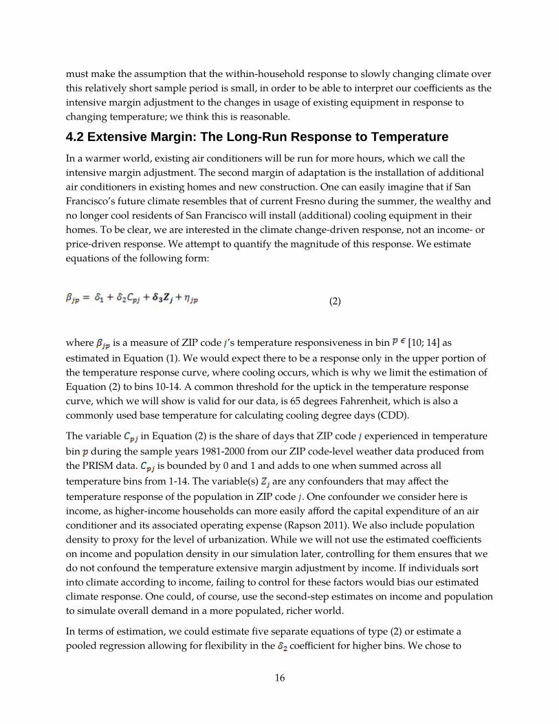
4.2 Extensive Margin: The Long-Run Response to Temperature

In a warmer world, existing air conditioners will be run for more hours, which we call the

intensive margin adjustment. The second margin of adaptation is the installation of additional

air conditioners in existing homes and new construction. One can easily imagine that if San

Francisco’s future climate resembles that of current Fresno during the summer, the wealthy and

no longer cool residents of San Francisco will install (additional) cooling equipment in their

homes. To be clear, we are interested in the climate change-driven response, not an income- or

price-driven response. We attempt to quantify the magnitude of this response. We estimate

equations of the following form:

(2)

where is a measure of ZIP code ’s temperature responsiveness in bin [10; 14] as

estimated in Equation (1). We would expect there to be a response only in the upper portion of

the temperature response curve, where cooling occurs, which is why we limit the estimation of

Equation (2) to bins 10-14. A common threshold for the uptick in the temperature response

curve, which we will show is valid for our data, is 65 degrees Fahrenheit, which is also a

commonly used base temperature for calculating cooling degree days (CDD).

The variable in Equation (2) is the share of days that ZIP code experienced in temperature

bin during the sample years 1981-2000 from our ZIP code-level weather data produced from

the PRISM data. is bounded by 0 and 1 and adds to one when summed across all

temperature bins from 1-14. The variable(s) are any confounders that may affect the

temperature response of the population in ZIP code . One confounder we consider here is

income, as higher-income households can more easily afford the capital expenditure of an air

conditioner and its associated operating expense (Rapson 2011). We also include population

density to proxy for the level of urbanization. While we will not use the estimated coefficients

on income and population density in our simulation later, controlling for them ensures that we

do not confound the temperature extensive margin adjustment by income. If individuals sort

into climate according to income, failing to control for these factors would bias our estimated

climate response. One could, of course, use the second-step estimates on income and population

to simulate overall demand in a more populated, richer world.

In terms of estimation, we could estimate five separate equations of type (2) or estimate a

pooled regression allowing for flexibility in the coefficient for higher bins. We chose to

17

estimate a pooled model, which restricts the coefficients on income and population density to be

identical for all bins, yet controls for bin dummies. This provided more stable estimation results

than estimating separate equations. The bin dummies control for the fact that each bin contains

the response coefficients for a different collection of ZIP codes. This arises, as we mentioned

above, because we do not have temperature coverage in all bins for all ZIP codes. Finally, we

estimate Equation (2) via Ordinary Least Squares with heteroskedasticity robust standard

errors, as the dependent variables are estimated coefficients and do not have constant variance.

Running weighted least squares does not significantly change the results, yet the least squares

estimates are more stable.

5: Estimation Results

5.1 Intensive Margin: The Usage Response to Temperature

As discussed in the previous section, we estimate Equation (1) for each of the 1,165 ZIP codes

that have more than 1,000 bills. While we cannot feasibly present all of the estimated

temperature response functions (which are comprised of up to 13 parameter estimates each), we

can display the distribution of the temperature response curves in a fan plot, which is shown in

Figure (3).3

3 For some ZIP codes the coverage in the extreme temperature bins is very small. After visual inspection

of all response curves we have dropped coefficients in only the extreme temperature bins with insufficient

data coverage for simulation purposes.

18

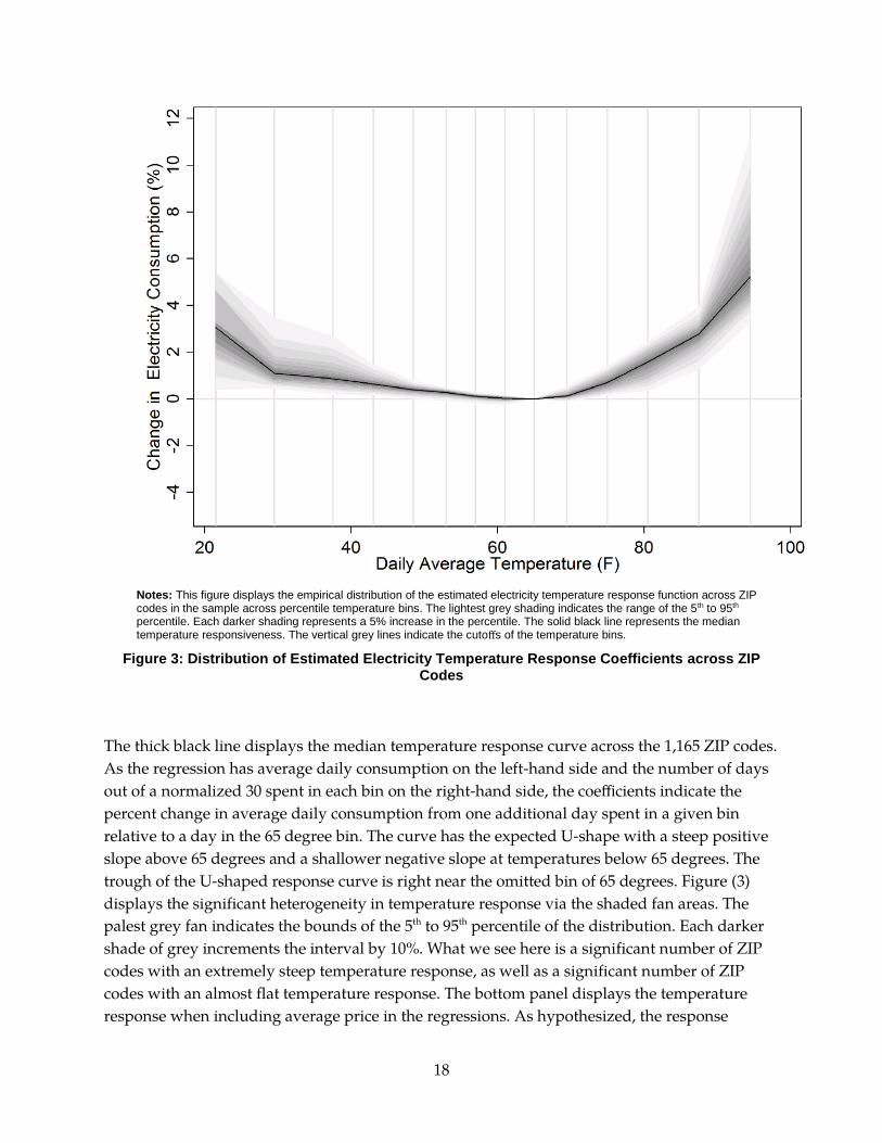
Notes: This figure displays the empirical distribution of the estimated electricity temperature response function across ZIP codes in the sample across percentile temperature bins. The lightest grey shading indicates the range of the 5th to 95th percentile. Each darker shading represents a 5% increase in the percentile. The solid black line represents the median temperature responsiveness. The vertical grey lines indicate the cutoffs of the temperature bins.

Figure 3: Distribution of Estimated Electricity Temperature Response Coefficients across ZIP Codes

The thick black line displays the median temperature response curve across the 1,165 ZIP codes.

As the regression has average daily consumption on the left-hand side and the number of days

out of a normalized 30 spent in each bin on the right-hand side, the coefficients indicate the

percent change in average daily consumption from one additional day spent in a given bin

relative to a day in the 65 degree bin. The curve has the expected U-shape with a steep positive

slope above 65 degrees and a shallower negative slope at temperatures below 65 degrees. The

trough of the U-shaped response curve is right near the omitted bin of 65 degrees. Figure (3)

displays the significant heterogeneity in temperature response via the shaded fan areas. The

palest grey fan indicates the bounds of the 5th to 95th percentile of the distribution. Each darker

shade of grey increments the interval by 10%. What we see here is a significant number of ZIP

codes with an extremely steep temperature response, as well as a significant number of ZIP

codes with an almost flat temperature response. The bottom panel displays the temperature

response when including average price in the regressions. As hypothesized, the response

19

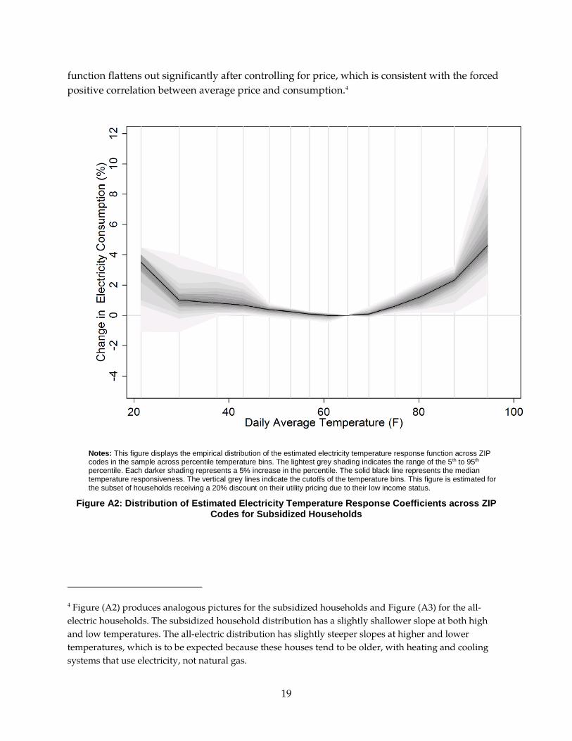
function flattens out significantly after controlling for price, which is consistent with the forced

positive correlation between average price and consumption.4

Notes: This figure displays the empirical distribution of the estimated electricity temperature response function across ZIP codes in the sample across percentile temperature bins. The lightest grey shading indicates the range of the 5th to 95th percentile. Each darker shading represents a 5% increase in the percentile. The solid black line represents the median temperature responsiveness. The vertical grey lines indicate the cutoffs of the temperature bins. This figure is estimated for the subset of households receiving a 20% discount on their utility pricing due to their low income status.

Figure A2: Distribution of Estimated Electricity Temperature Response Coefficients across ZIP Codes for Subsidized Households

4 Figure (A2) produces analogous pictures for the subsidized households and Figure (A3) for the all-

electric households. The subsidized household distribution has a slightly shallower slope at both high

and low temperatures. The all-electric distribution has slightly steeper slopes at higher and lower

temperatures, which is to be expected because these houses tend to be older, with heating and cooling

systems that use electricity, not natural gas.

20

Notes: This figure displays the empirical distribution of the estimated electricity temperature response function across ZIP codes in the sample across percentile temperature bins. The lightest grey shading indicates the range of the 5th to 95th percentile. Each darker shading represents a 5% increase in the percentile. The solid black line represents the median temperature responsiveness. The vertical grey lines indicate the cutoffs of the temperature bins. This figure is estimated for the subset of households identified as all–electric by the utilities.

Figure A3: Distribution of Estimated Electricity Temperature Response Coefficients across ZIP Codes for All-Electric Households

21

Notes: This figure displays the empirical distribution of the estimated electricity temperature response function across ZIP codes in the sample across percentile temperature bins. The lightest grey shading indicates the range of the 5th to 95th percentile. Each darker shading represents a 5% increase in the percentile. The solid black line represents the median temperature responsiveness. The vertical grey lines indicate the cutoffs of the temperature bins.

Figure 4: Distribution of Estimated Natural Gas Temperature Response Coefficients across ZIP

Codes

Figure (4) displays the analogous results for the natural gas regressions, also excluding price

from the regressions. Because space heating is the only major ambient temperature-sensitive use

of natural gas in residences, we would expect a downward sloping line in temperature at low

temperatures and a relatively flat response curve at higher temperatures. Figure (4)

impressively displays exactly that. There is quite a bit of variation in slope across ZIP codes, yet

the median response is exactly as expected and flattens out at almost exactly 65 degrees

Fahrenheit.

5.2 Extensive Margin: The Long-Run Electricity Consumption Response to Temperature

As discussed in Section 4.2, we exploit the 1,165 estimated electricity temperature response

curves and examine whether we can explain variation in temperature response at high

temperatures through cross-sectional variation in “climate” as well as income and population

density.

22

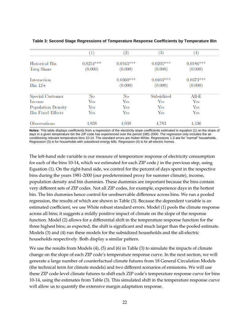
Table 3: Second Stage Regressions of Temperature Response Coefficients by Temperature Bin

Notes: This table displays coefficients from a regression of the electricity slope coefficients estimated in equation (1) on the share of days in a given temperature bin the ZIP code has experienced over the period 1981-2000. The regression only includes the air conditioning relevant temperature bins 10-14. The standard errors are Huber-White. Regressions 1-2 are for “normal" households. Regression (3) is for households with subsidized energy bills. Regression (4) is for all-electric homes.

The left-hand side variable is our measure of temperature response of electricity consumption

for each of the bins 10-14, which we estimated for each ZIP code in the previous step, using

Equation (1). On the right-hand side, we control for the percent of days spent in the respective

bins during the years 1981-2000 (our predetermined proxy for summer climate), income,

population density and bin dummies. These dummies are important because the bins contain

very different sets of ZIP codes. Not all ZIP codes, for example, experience days in the hottest

bin. The bin dummies hence control for unobservable difference across bins. We run a pooled

regression, the results of which are shown in Table (3). Because the dependent variable is an

estimated coefficient, we use White robust standard errors. Model (1) pools the climate response

across all bins; it suggests a mildly positive impact of climate on the slope of the response

function. Model (2) allows for a differential shift in the temperature response function for the

three highest bins; as expected, the shift is significant and much larger than the pooled estimate.

Models (3) and (4) run these models for the subsidized households and the all-electric

households respectively. Both display a similar pattern.

We use the results from Models (4), (5) and (6) in Table (3) to simulate the impacts of climate

change on the slope of each ZIP code’s temperature response curve. In the next section, we will

generate a large number of counterfactual climate futures from 18 General Circulation Models

(the technical term for climate models) and two different scenarios of emissions. We will use

these ZIP code-level climate futures to shift each ZIP code’s temperature response curve for bins

10-14, using the estimates from Table (3). This simulated shift in the temperature response curve

will allow us to quantify the extensive margin adaptation response.

23

6: Electricity and Natural Gas Consumption Simulations

In this section, we simulate the impacts of climate change on electricity and then natural gas

consumption under two different emissions scenarios using 18 different climate models from

the latest round of the IPCC assessments (AR5, CMIP5) in their downscaled form. For

electricity, we conduct three different simulations. All Simulations hold overall population

growth and incomes constant. The first set of simulations only simulate electricity consumption

per household using the first-stage estimates, which do not allow for changes in the extensive

margin. In a second simulation, we incorporate the extensive margin adjustments from the

previous section. For each simulation, we can calculate the trajectory of aggregate electricity

consumption from the residential sector until the year 2099, which is standard in the climate

change literature. We provide simulated impacts for the periods 2020-2039, 2040-2059, 2060-

2079 and 2080-2099.

In our simulations, we make one key assumption. For natural gas, we only use the intensive

margin simulations, because one would not expect households to install more efficient or fewer

heaters in response to climate change. We would expect existing equipment to be operated less

frequently. But one would not install a more efficient and costly heater which is going to be

used less due to climate change.

6.1 Temperature Simulations

The simulation for this section uses the climate response parameters estimated in Section 5.1.

Using these estimates as the basis of our simulation has several strong implications. Using only

the first stage parameters via Equation (1) implies that the climate responsiveness of

consumption within climate zones remains constant throughout the century.

As is standard in this literature, the counterfactual climate is generated by a general circulation

model (GCM). These numerical simulation models generate predictions of past and future

climate under different scenarios of atmospheric greenhouse gas (GHG) concentrations. The

quantitative projections of global climate change conducted under the auspices of the IPCC’s

fifth assessment report (AR5) and applied in this study are based on the so-called “RCP 4.5” and

“RCP 8.5” scenarios. The number after the RCP stands for the likely increase in forcing from the

scenario by end of century relative to preindustrial values, in Watts per square meter. In terms

more familiar to most economists, RCP 4.5 is expected to result in warming of 1.8 °C, with a

likely range of 1.1. to 2.6 °C. This is a very optimistic scenario, as attaining a goal of warming

less than 2 degrees is unlikely. RCP 8.5 is the worst case scenario and is expected to result in

warming of 3.7 °C, with a likely range of 2.6 to 4.8 °C.

We simulate consumption for each scenario using the 18 downscaled GCMs from the IPCC’s

CMIP5 database. The downscaled temperature scenarios were drawn from a statistical

downscaling exercise based on the Coupled Model Intercomparison Project 5 (Taylor et al. 2012)

utilizing a modification (Hegewisch and Abatzoglou, 2015) of the Multivariate Adaptive

24

Constructed Analogs (Abatzoglou and Brown, 2012) method with the Livneh (Livneh et al.,

2013) observational dataset as training data. These were provided to us by the MACA project at

the University of Idaho. We matched the fine scale grids of the downscaled climate data to ZIP

codes in the same fashion that we matched the PRISM weather grids. We calculated future

climate by adding the predicted change in monthly temperature for each model, scenario and

period to our baseline weather data, in order to avoid local biases, as the MACA project does

not use the same weather data as its training data set.5

To obtain estimates for a percent increase in electricity consumption for the representative

household in ZIP code and period , we use the following relation:

(3)

5 A detailed description of the climate model output is available at

http://maca.northwestknowledge.net/.

25

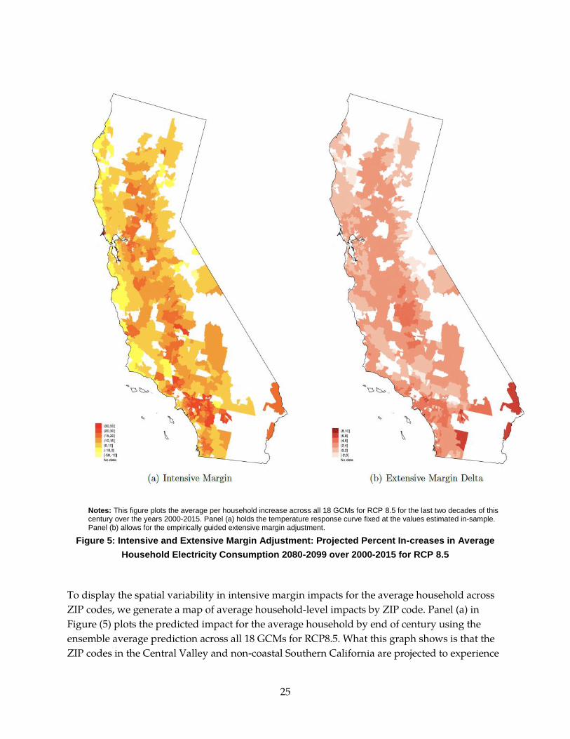
Notes: This figure plots the average per household increase across all 18 GCMs for RCP 8.5 for the last two decades of this century over the years 2000-2015. Panel (a) holds the temperature response curve fixed at the values estimated in-sample. Panel (b) allows for the empirically guided extensive margin adjustment.

Figure 5: Intensive and Extensive Margin Adjustment: Projected Percent In-creases in Average

Household Electricity Consumption 2080-2099 over 2000-2015 for RCP 8.5

To display the spatial variability in intensive margin impacts for the average household across

ZIP codes, we generate a map of average household-level impacts by ZIP code. Panel (a) in

Figure (5) plots the predicted impact for the average household by end of century using the

ensemble average prediction across all 18 GCMs for RCP8.5. What this graph shows is that the

ZIP codes in the Central Valley and non-coastal Southern California are projected to experience

26

the largest increases in household electricity consumption. This is due to the combination of the

slope of the temperature response function and projected warming from the GCMs. These

projections ignore potential extensive margin impacts, which we turn to next.6

6 Figure (A4) displays the projected increases in household residential electricity consumption across the

approxi-mately 1,200 ZIP codes for each of the four projection periods and the 18 GCMs for RCP 8.5. The

top panel displays this for intensive margin impacts only, while the bottom panel adds the extensive

margin response. The box plots display tremendous variation across time (the box and whiskers plots for

each model are shown in increasing temporal order for each model), across models, and within models. It

is quite clear that median impacts are increasing over time and impacts range from the negative teens to

increases approaching 50% for some ZIP codes. We trim the distribution of estimated impacts at the top

and bottom because some point estimates are too large to be credible. This has to do with a lack of

precision for some zip codes with very few observations in the extreme bins. We censor the slope

coefficients to be less than 0.2 in absolute value and the projected impacts to be less than 50%.

27

Figure A4: Intensive margin [Top Panel] and Extensive Margin [Bottom Panel] per household

impacts across ZIP codes and Climate Models.

28

For each ZIP code, climate model and scenario, we calculate the simulated shift of the

temperature response curve using Model (2) in Table (3). As the temperature distribution shifts

to the right for the vast majority of ZIP codes in California, a higher share of days in the higher

bins is projected under both climate change scenarios for most models. We use these extensive

margin adjusted response functions to simulate impacts of climate change on electricity

consumption. Panel (b) in Figure (5) displays the impacts on the average household in a ZIP

code using the ensemble average of GCMs and RCP 8.5 by end of century across the state for

the extensive margin adaptation. It is important to note that this figure plots the “delta” from

the intensive margin results. It indicates a noticeable increase in consumption across the state

relative to the intensive margin only, shown in Panel (a). The right panel shows that these

extensive margin impacts will be felt most strongly in the Central Valley and non-coastal areas

of Southern California.7

Table 4: Projected Percent Changes in Residential Electricity Consumption

Notes: This table displays the simulated percent increase in total residential electricity consumption relative to 2000-2015 climate for the two IPCC Representative Concentration Pathways with low emissions (4.5) and high emissions (8.5). Columns (1) and (2), indicate simulated increases for normal households Columns (3) and (4) simulate increases for subsidized households. Columns (5) and (6) simulate changes for households which are all-electric. Columns (7) and (8) display the impacts on natural gas consumption for households with gas bills.

7 The bottom panel in Figure (A4) displays the same box and whisker plots as we did for the intensive

margin simulations earlier, but now incorporates the extensive margin changes. What stands out from

this graph is an almost uniform upward shift in the medians across models and increased variability

across models - especially at the high end.

29

While these maps are instructive, it is hard to determine the size of the overall impact of

allowing for extensive margin adjustment. Table (4) therefore shows the overall population-

weighted increases in total electricity consumption averaged across the 18 climate models and

for both RCPs - with and without extensive margin adjustments. The first thing to notice from

this table is that accounting for the extensive margin adjustments results in a significant

difference in simulated impacts, which is consistent with the findings in Davis and Gertler

(2015) for Mexico. For RCP4.5 by the end of the century, accounting for extensive margin

impacts increases the estimated impacts by 30%. The second noteworthy fact is that the

estimated impacts for electricity consumption are relatively small even until 2059 - strictly less

than 5% even for the worst case scenario incorporating extensive margin adjustment. In terms

of the electricity planners’ time horizon, the magnitude of the impacts falls within the noise. By

the end of the century, the impacts are larger, yet their magnitudes are small enough that not

overly optimistic assumptions about technological change related to energy efficiency should

more than offset these gains. A 14.7% increase in electricity consumption from “normal”

households - which is the largest effect we find - by end of century is about a 0.2% annual

growth rate. The results for low-income households are even smaller: a 14% increase for the

worst case scenario by the end of the century. The results for all–electric homes are much

smaller. This makes sense because, for these homes, decreased heating will offset increases in air

conditioning demand.

For natural gas, however, we see more significant decreases in consumption, even by mid-

century. Under RCP8.5, consumption is expected to decrease by 10.4% by mid-century and by

end of century by 20.5%. Again, the end of century is a long ways away and beyond the utility

planners’ horizon, but this raises the question of whether the savings from natural gas are

bigger than the projected increases in electricity consumption in this counterfactual world. The

Energy Information Administration (EIA) states that California homes used 0.287 quadrillion

BTU of electricity and 0.439 quadrillion BTU of natural gas in 2009. If we use the projected

percentage changes from Table (4), we arrive at the conclusion that climate change is simulated

to lead to a 0.039 quad BTU net decrease in final energy consumption for the residential sector

in California. This does of course not account for the generation and transmission losses

incurred in the electricity sector. We will discuss the limitations of this simulation in the

conclusions.

7: Conclusions

In the residential sector, one of the most widely discussed modes of adaptation to higher

temperatures due to climate change is the increased demand for cooling and decreased demand

for heating in the built environment. Due to its mild climate and heavy reliance on natural gas,

California’s residential sector uses relatively little electricity for heating. It is therefore expected

that the demand for electricity will increase as households operate existing air conditioners

more frequently, and in many regions will install air conditioners where there currently are few.

30

This paper provides reduced form estimates of changes in electricity consumption due to

increased use of installed cooling equipment under a hotter climate. The study adds to the

literature by incorporating the change in temperature responsiveness due to likely increases in

air conditioner penetration under climate change, using a two-stage method. The advantage of

the proposed method lies in its relative simplicity and the fact that it only requires data on

electricity consumption and not on installed cooling equipment.

We show that accounting for extensive margin adjustments will lead to statistically and

economically significantly higher projections of electricity consumption. However, by

estimating the response of natural gas consumption to higher temperatures, we also show that

the projected increases in final electricity consumption are more than offset by savings in

directly consumed natural gas.

It is important to keep in mind several caveats. These are simulations, not forecasts. We think of

the results provided in this paper as imposing end of century climate on a current day

economy. Many other drivers of energy consumption will change. What our paper shows is the

business as usual path, which mitigation strategy has to work against. We do not and cannot

model changes in electricity consumption due to improvements in the efficiency of heating and

cooling equipment and/or buildings. These effects will offset some or all of the increases in

electricity consumption outlined in this paper and will amplify the natural gas savings. Further,

the extensive margin adjustments in this paper cannot meaningfully control for changes in

urban form, urban heat island effects, or other variables potentially leading to a higher

response, which may be correlated with temperature. We leave the study of these effects to

future work.

31

8: References

Abatzoglou, John T., and Timothy J. Brown. 2012. “A comparison of statistical downscaling

methods suited for wildfire applications.” International Journal of Climatology 32.5: 772-780.

Albouy, D., Graf, W. F., Kellogg, R., & Wolff, H. 2013. Climate amenities, climate change, and

American quality of life (No. w18925). National Bureau of Economic Research.

Anthoff, David, and Richard Tol. 2014. The Climate Framework for Uncertainty, Negotiation and

Distribution (FUND). Technical Description.

Aroonruengsawat, Anin, and Maximilian Auffhammer. 2012. Correction: Impacts of Climate

Change on Residential Electricity Consumption: Evidence From Billing Data. California En-ergy

Commission White Paper.

Auffhammer, Maximilian and Anin Aroonruengsawat. 2012b Hotspots of climate-driven increases

in residential electricity demand: A simulation exercise based on household level billing data

for California. California Energy Commission.

Auffhammer, Maximilian, Patrick Baylis, and Catherine H. Hausman. 2017. “Climate change is

projected to have severe impacts on the frequency and intensity of peak electricity demand

across the United States.” Proceedings of the National Academy of Sciences: 201613193.

Auffhammer, Maximilian, and Erin T. Mansur. 2014. “Measuring climatic impacts on energy

consumption: A review of the empirical literature.” Energy Economics 46: 522-530.

Auffhammer, M. and Vincent, J. R. 2012. Unobserved time effects confound the identification of

climate change impacts. Proceedings of the National Academy of Sciences, 109(30), 11973-11974.

Barreca, Alan, Karen Clay, Olivier Deschenes, Michael Greenstone, Joseph S. Shapiro. 2016.

“Adapting to Climate Change: The Remarkable Decline in the U.S. Temperature-Mortality

Relationship over the 20th Century.” Journal of Political Economy. 124(1): 105-159

Baxter, L. W., and K. Calandri. 1992. “Global warming and electricity demand: A study of

California.” Energy Policy 20(3): 233-244.

BEA (Bureau of Economic Analysis). 2008. Regional Economic Accounts. Washington, D.C.

www.bea.gov/regional/spi/default.cfm?series=summary.

Biddle, Jeff. 2008. “Explaining the spread of residential air conditioning, 1955-1980.” Explorations in

Economic History 45: 402-423.

Bigano, Andrea, Jacqueline M. Hamilton, and Richard SJ Tol. 2006. The impact of climate on

holiday destination choice.” Climatic Change 76.3-4: 389-406.

Burke, Marshall and Kyle Emerick. 2016. “Adaptation to climate change: Evidence from US

agriculture”. American Economic Journal – Economic Policy, 8(3), 106-140.

32

Butler, Ethan E., and Peter Huybers. 2013. “Adaptation of US maize to temperature variations.”

Nature Climate Change 3.1: 68-72.

Carleton, Tamma A., and Solomon M. Hsiang. 2016. “Social and economic impacts of climate.”

Science 353.6304 : aad9837.

Cline, W. R. 1992. The economics of global warming. Washington: Institute for International

Economics.

Crowley, C., and F. Joutz. 2003. Hourly electricity loads: Temperature elasticities and climate

change. In 23rd U.S. Association of Energy Economics North American Conference.

Davis, Lucas W. and Paul J. Gertler. 2015 “Contribution of air conditioning adoption to future

energy use under global warming” PNAS doi:10.1073/pnas.1423558112

Dell, Melissa, Benjamin F. Jones, and Benjamin A. Olken. 2012. “Temperature shocks and economic

growth: Evidence from the last half century.” American Economic Journal: Macroeconomics 4.3:

66-95.

Dell, Melissa, Benjamin F. Jones, and Benjamin A. Olken. 2014. “What do we learn from the

weather? The new climate–economy literature.” Journal of Economic Literature 52.3: 740-798.

Deschenes, O., and M. Greenstone. 2011. “Climate Change, Mortality and Adaptation: Evidence

from annual fluctuations in weather in the U.S.” American Economic Journal: Applied

Economics. 3: 152-185.

Energy Information Administration (EIA). 2008. State Energy Data System. Washington, D.C.

http://www.eia.doe.gov/emeu/states/_seds.html.

Energy Information Administration. 2011. “Air conditioning in nearly 100 million U.S. homes.”

http://www.eia.gov/consumption/residential/reports/air_conditioning09. cfm?src=email.

Feng, S., Oppenheimer, M., and Schlenker, W. 2012. Climate change, crop yields, and internal

migration in the United States (No. w17734). National Bureau of Economic Research.

Fisher, Anthony C., et al. 2012. “The economic impacts of climate change: evidence from

agricultural output and random fluctuations in weather: comment.” The American Economic

Review 102.7: 3749-3760.

Franco, G., and A. Sanstad. 2008. “Climate change and electricity demand in California.” Climatic

Change 87:139-151.

Hanemann, W. 1984. “Discrete/Continuous Models of Consumer Demand.” Econometrica 52: 541-

561.

Heutel, Garth, Nolan H. Miller and David Molitor. 2017. Adaptation and the Mortality Effects of

Temperature Across U.S. Climate Regions. NBER Working Paper #23271

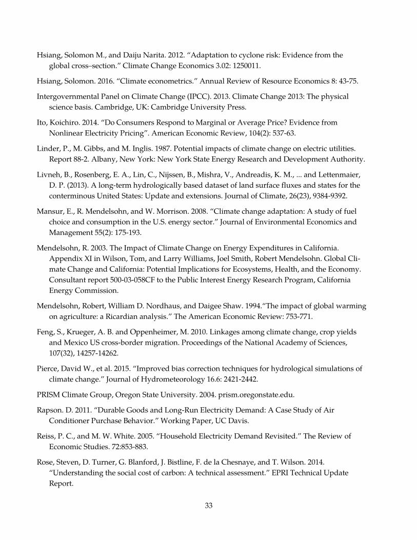
33

Hsiang, Solomon M., and Daiju Narita. 2012. “Adaptation to cyclone risk: Evidence from the

global cross–section.” Climate Change Economics 3.02: 1250011.

Hsiang, Solomon. 2016. “Climate econometrics.” Annual Review of Resource Economics 8: 43-75.

Intergovernmental Panel on Climate Change (IPCC). 2013. Climate Change 2013: The physical

science basis. Cambridge, UK: Cambridge University Press.

Ito, Koichiro. 2014. “Do Consumers Respond to Marginal or Average Price? Evidence from

Nonlinear Electricity Pricing”. American Economic Review, 104(2): 537-63.

Linder, P., M. Gibbs, and M. Inglis. 1987. Potential impacts of climate change on electric utilities.

Report 88-2. Albany, New York: New York State Energy Research and Development Authority.

Livneh, B., Rosenberg, E. A., Lin, C., Nijssen, B., Mishra, V., Andreadis, K. M., ... and Lettenmaier,

D. P. (2013). A long-term hydrologically based dataset of land surface fluxes and states for the

conterminous United States: Update and extensions. Journal of Climate, 26(23), 9384-9392.

Mansur, E., R. Mendelsohn, and W. Morrison. 2008. “Climate change adaptation: A study of fuel

choice and consumption in the U.S. energy sector.” Journal of Environmental Economics and

Management 55(2): 175-193.

Mendelsohn, R. 2003. The Impact of Climate Change on Energy Expenditures in California.

Appendix XI in Wilson, Tom, and Larry Williams, Joel Smith, Robert Mendelsohn. Global Cli-

mate Change and California: Potential Implications for Ecosystems, Health, and the Economy.

Consultant report 500-03-058CF to the Public Interest Energy Research Program, California

Energy Commission.

Mendelsohn, Robert, William D. Nordhaus, and Daigee Shaw. 1994.“The impact of global warming

on agriculture: a Ricardian analysis.” The American Economic Review: 753-771.

Feng, S., Krueger, A. B. and Oppenheimer, M. 2010. Linkages among climate change, crop yields

and Mexico US cross-border migration. Proceedings of the National Academy of Sciences,

107(32), 14257-14262.

Pierce, David W., et al. 2015. “Improved bias correction techniques for hydrological simulations of

climate change.” Journal of Hydrometeorology 16.6: 2421-2442.

PRISM Climate Group, Oregon State University. 2004. prism.oregonstate.edu.

Rapson. D. 2011. “Durable Goods and Long-Run Electricity Demand: A Case Study of Air

Conditioner Purchase Behavior.” Working Paper, UC Davis.

Reiss, P. C., and M. W. White. 2005. “Household Electricity Demand Revisited.” The Review of

Economic Studies. 72:853-883.

Rose, Steven, D. Turner, G. Blanford, J. Bistline, F. de la Chesnaye, and T. Wilson. 2014.

“Understanding the social cost of carbon: A technical assessment.” EPRI Technical Update

Report.

34

Rosenthal, D., H. Gruenspecht, and E. Moran. 1995. “Effects of global warming on energy use for

space heating and cooling in the United States.” The Energy Journal 16:77-96.

Sailor, D., and A. Pavlova. 2003. “Air conditioning market saturation and long-term response of

residential cooling energy demand to climate change.” Energy 28 (9): 941-51.

Sanstad, A., H. Johnson, N. Goldstein, and G. Franco. 2009. Long-Run Socioeconomic and

Demographic Scenarios for California. PIER Report CEC-500-2009-013-D.

Schlenker, W., and M. Roberts. 2006. “Nonlinear Effects of Weather on Corn Yields.” Review of

Agricultural Economics 28(3): 391-398.

Schlenker and Roberts. 2009. “Nonlinear Temperature Effects indicate Severe Damages to U.S. Crop

Yields under Climate Change.” Proceedings of the National Academy of Sciences, 106(37),

September 15 2009, p.15594-15598.

Taylor, Karl E., Ronald J. Stouffer, and Gerald A. Meehl. 2012. “An overview of CMIP5 and the

experiment design.” Bulletin of the American Meteorological Society 93.4: 485-498.

U.S. Environmental Protection Agency. 1989. “The potential effects of global climate change on the

United States.” Joel B. Smith and Dennis Tirpak, eds. Washington D.C.: Environmental

Protection Agency.

A-1

APPENDIX A: Tables and Figures

Table 1: Electricity and Natual Gas Bills by Utility

Notes: This table displays the total number of bills in our dataset. We drop electricity bills with average daily consumption less than 2kWh as well as solar homes. Further, the estimated models only include ZIP codes for which we have more than 1,000 bills.

Table 2: Summary Statistics for ZIP Codes In and Out of Sample

Notes: This table displays the mean observable characteristics of the ZIP codes in our sample and ZIP codes not in our sample with positive population. The t-test assumes unequal variances. The observable characteristics were purchased from zip-codes.com.

A-2

Table 3: Second Stage Regressions of Temperature Response Coefficients by Temperature Bin

Notes: This table displays coefficients from a regression of the electricity slope coefficients estimated in equation (1) on the share of days in a given temperature bin the ZIP code has experienced over the period 1981-2000. The regression only includes the air conditioning relevant temperature bins 10-14. The standard errors are Huber-White. Regressions 1-2 are for “normal" households. Regression (3) is for households with subsidized energy bills. Regression (4) is for all-electric homes.

Table 4: Projected Percent Changes in Residential Electricity Consumption

Notes: This table displays the simulated percent increase in total residential electricity consumption relative to 2000-2015 climate for the two IPCC Representative Concentration Pathways with low emissions (4.5) and high emissions (8.5). Columns (1) and (2), indicate simulated increases for normal households Columns (3) and (4) simulate increases for subsidized households. Columns (5) and (6) simulate changes for households which are all-electric. Columns (7) and (8) display the impacts on natural gas consumption for households with gas bills.

A-3

Notes: This figure displays the temperature response of electricity consumption in three fictional ZIP codes with differing climates - moderate, warm and hot. The bars at the bottom display the temperature (weather) distribution for the three ZIP codes. The colors of the response functions match the colors of the weather distribution(s). The figure displays that the hot ZIP code has a steeper temperature response at higher temperatures than the warm and moderate ZIP codes. The first step in the estimation identifies the ZIP code specific temperature response curves using household level data. The second estimation step estimates the effect of climate (average time spent in a portion of the temperature spectrum) on the slope of the response curves across ZIP codes for the air conditioning relevant portion of the temperature spectrum.

Figure 1: Conceptual Identification of Short and Long Run Response

A-4

Figure 2: California's Summer (June-August) and Winter (December-February) Climate: Average Daily Temperature 1981-2015

A-5

Notes: This figure displays the empirical distribution of the estimated electricity temperature response function across ZIP codes in the sample across percentile temperature bins. The lightest grey shading indicates the range of the 5th to 95th percentile. Each darker shading represents a 5% increase in the percentile. The solid black line represents the median temperature responsiveness. The vertical grey lines indicate the cutoffs of the temperature bins.

Figure 3: Distribution of Estimated Electricity Temperature Response Coefficients across ZIP Codes

A-6

Notes: This figure displays the empirical distribution of the estimated electricity temperature response function across ZIP codes in the sample across percentile temperature bins. The lightest grey shading indicates the range of the 5th to 95th percentile. Each darker shading represents a 5% increase in the percentile. The solid black line represents the median temperature responsiveness. The vertical grey lines indicate the cutoffs of the temperature bins.

Figure 4: Distribution of Estimated Natural Gas Temperature Response Coefficients across ZIP Codes

A-7

Notes: This figure plots the average per household increase across all 18 GCMs for RCP 8.5 for the last two decades of this century over the years 2000-2015. Panel (a) holds the temperature response curve fixed at the values estimated in-sample. Panel (b) allows for the empirically guided extensive margin adjustment.

Figure 5: Intensive and Extensive Margin Adjustment: Projected Percent In-creases in Average Household Electricity Consumption 2080-2099 over 2000-2015 for RCP 8.5

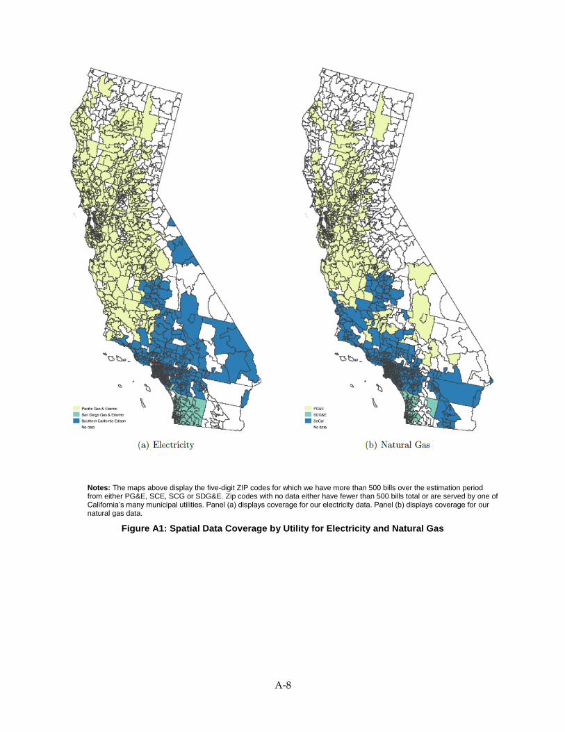
A-8

Notes: The maps above display the five-digit ZIP codes for which we have more than 500 bills over the estimation period from either PG&E, SCE, SCG or SDG&E. Zip codes with no data either have fewer than 500 bills total or are served by one of California’s many municipal utilities. Panel (a) displays coverage for our electricity data. Panel (b) displays coverage for our natural gas data.

Figure A1: Spatial Data Coverage by Utility for Electricity and Natural Gas

A-9

Notes: This figure displays the empirical distribution of the estimated electricity temperature response function across ZIP codes in the sample across percentile temperature bins. The lightest grey shading indicates the range of the 5th to 95th percentile. Each darker shading represents a 5% increase in the percentile. The solid black line represents the median temperature responsiveness. The vertical grey lines indicate the cutoffs of the temperature bins. This figure is estimated for the subset of households receiving a 20% discount on their utility pricing due to their low income status.

Figure A2: Distribution of Estimated Electricity Temperature Response Coeffi-cients across ZIP Codes for Subsidized Households

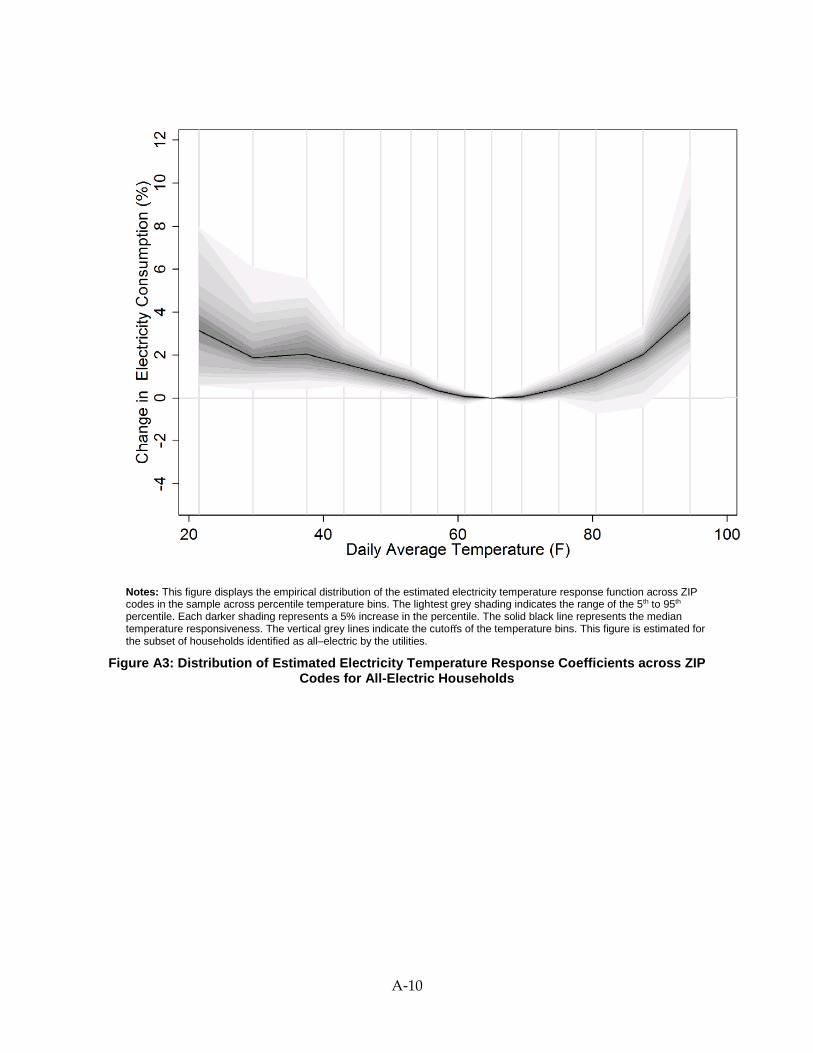
A-10

Notes: This figure displays the empirical distribution of the estimated electricity temperature response function across ZIP codes in the sample across percentile temperature bins. The lightest grey shading indicates the range of the 5th to 95th percentile. Each darker shading represents a 5% increase in the percentile. The solid black line represents the median temperature responsiveness. The vertical grey lines indicate the cutoffs of the temperature bins. This figure is estimated for the subset of households identified as all–electric by the utilities.

Figure A3: Distribution of Estimated Electricity Temperature Response Coefficients across ZIP Codes for All-Electric Households

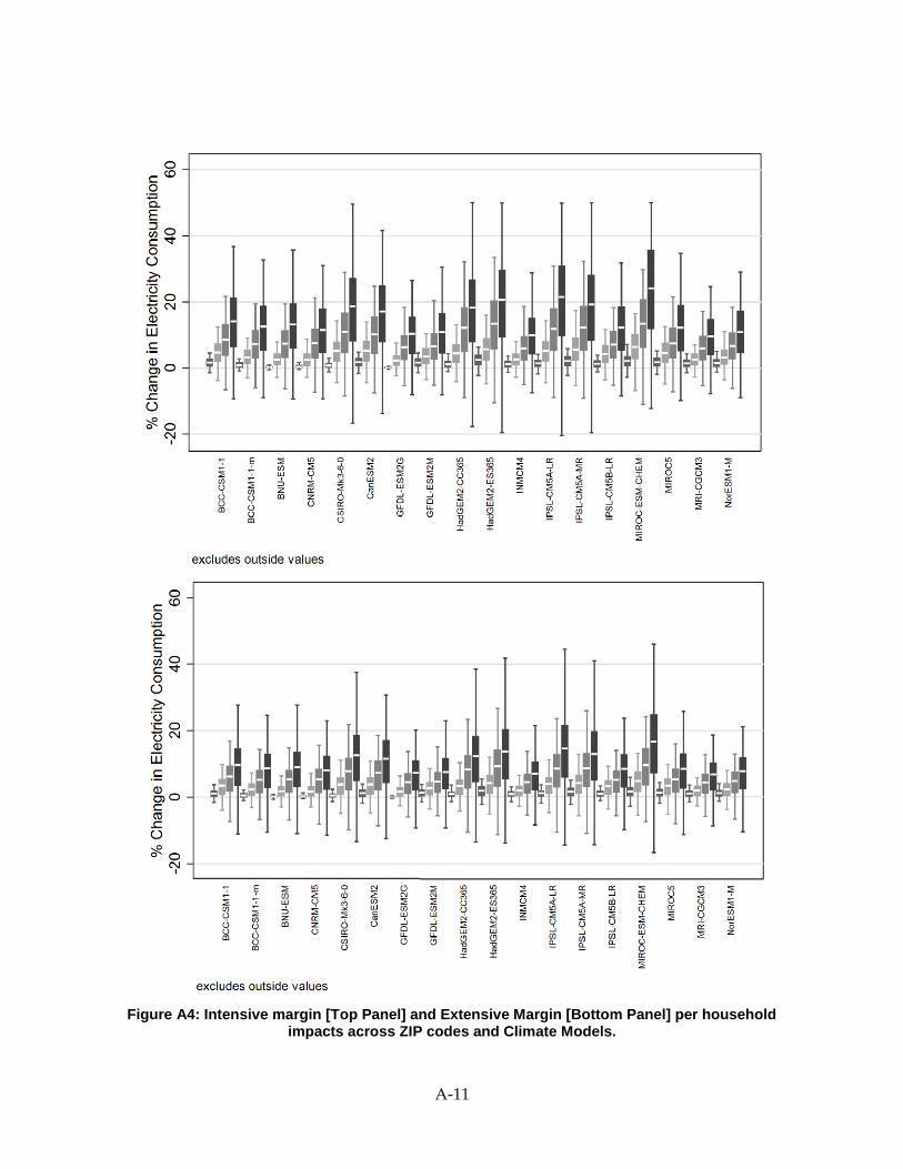
A-11

Figure A4: Intensive margin [Top Panel] and Extensive Margin [Bottom Panel] per household impacts across ZIP codes and Climate Models.