cmput 340 modeling kinematics for robots humans...
TRANSCRIPT
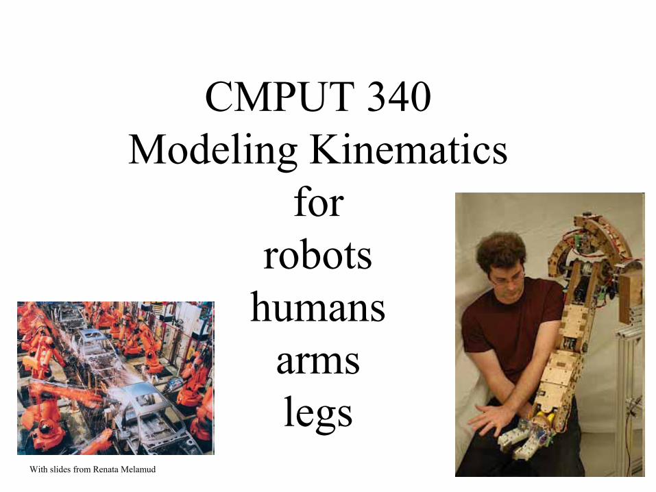
CMPUT 340 Modeling Kinematics
for robots
humans arms
legsWith slides from
Renata
Melamud

What a robot arm and hand can do
•
Martin 1992-’97 PhD work

What a robot arm and hand can do
•
Camilo 2011-17 PhD work

Robotics field . .
•
6 Million mobile robots–
From $100 roomba to $millions Mars rovers
•
1 million robot arms–
Usually $20,000-100,000, some millions
•
Value of industrial robotics: $25 billion•
Arms crucial for these industries:–
Automotive (Welding, painting, some assembly)
–
Electronics (Placing tiny components on PCB)–
General: Pack boxes, move parts from conveyor to machines
http://www.youtube.com/watch?v=DG6A1Bsi-lg

An classic arm -
The PUMA 560
The PUMA 560 has
SIX
revolute jointsA revolute joint has ONE degree of freedom ( 1 DOF) that is defined by its angle
1
2 3
4
There are two more joints on the end effector
(the gripper)
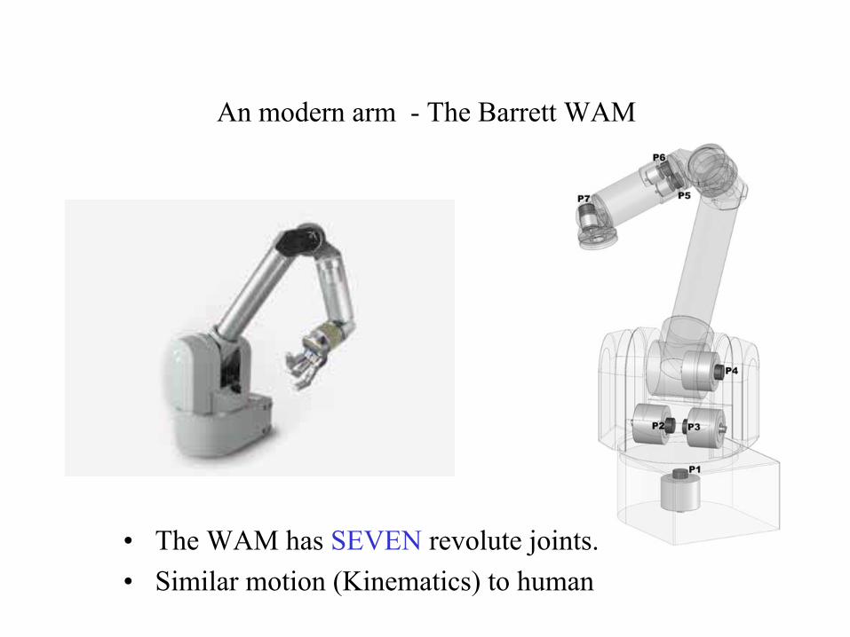
An modern arm -
The Barrett WAM
•
The WAM has SEVEN
revolute joints. •
Similar motion (Kinematics) to human

UA Robotics Lab platform 2 arm mobile manipulator
•
2 WAM arms, steel cable transmission and drive•
Segway mobile platform
•
2x Quad core computer platform.•
Battery powered, 4h run time.

•
Robotics challenges
Navigation ‘05Manipulation ‘11-14
Humanoids ’12-
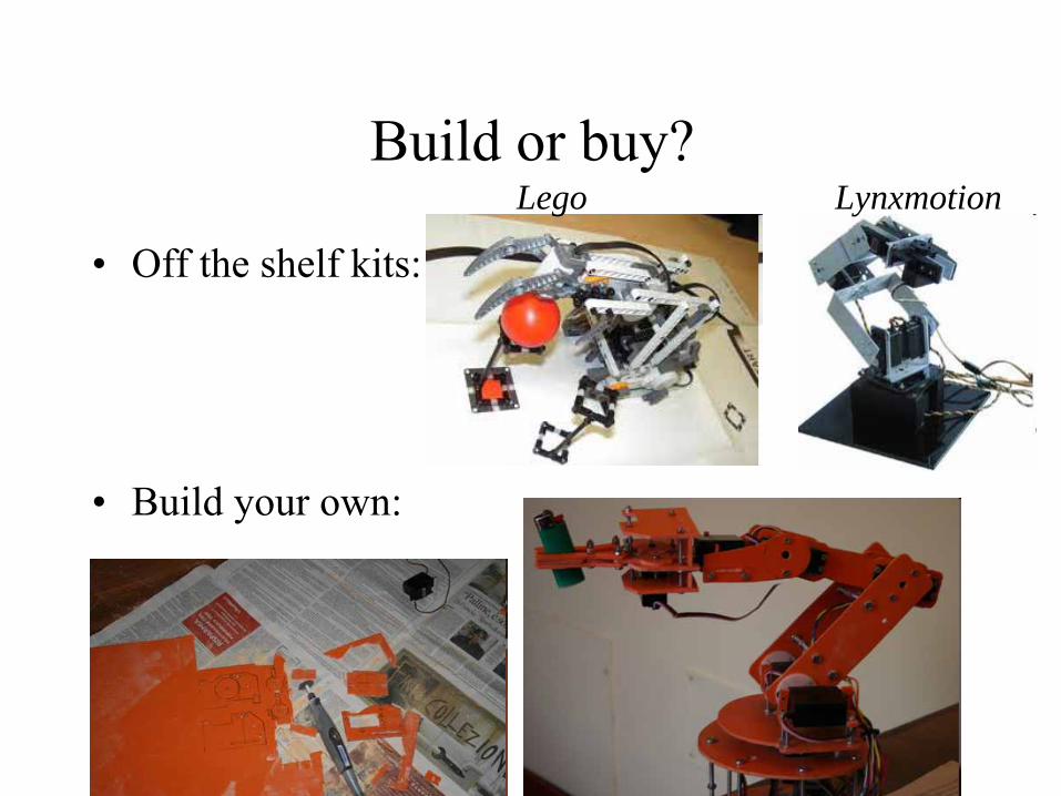
Build or buy?
•
Off the shelf kits:
•
Build your own:
Lego Lynxmotion
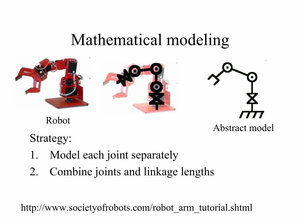
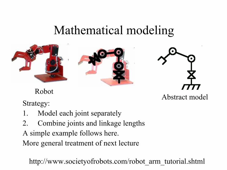
Mathematical modeling
Strategy: 1.
Model each joint separately
2.
Combine joints and linkage lengths
RobotAbstract model
http://www.societyofrobots.com/robot_arm_tutorial.shtml

Other basic joints
Spherical Joint3 DOF ( Variables -
Υ1
, Υ2
, Υ3
)
Revolute Joint1 DOF ( Variable -
Υ)
Prismatic Joint1 DOF (linear) (Variables -
d)

Example Matlab
robot
Successive translation and rotation
% robocop Simulates a 3 joint robot
function Jpos = robocop(theta1,theta2,theta3,L1,L2,L3,P0)
Rxy1 = [cos(theta1) sin(theta1) 0 -sin(theta1) cos(theta1) 0 0 0 1];
Rxz2 = [cos(theta2) 0 sin(theta2) 0 1 0 -sin(theta2) 0 cos(theta2)];
Rxz3 = [cos(theta3) 0 sin(theta3) 0 1 0 -sin(theta3) 0 cos(theta3)];
P1 = P0 + Rxy1*[L1 0 0]';P2 = P1 + Rxy1*Rxz2*[L2 0 0]';P3 = P2 + Rxy1*Rxz2*Rxz3*[L3 0 0]';Jpos = [P0 P1 P2 P3];
Mathematical modeling
Strategy: 1.
Model each joint separately
2. Combine joints and linkage lengths
A simple example follows here.More general treatment of next lecture
RobotAbstract model
http://www.societyofrobots.com/robot_arm_tutorial.shtml

Simple example: Modeling of a 2DOF planar manipulator
•
Move from ‘home’ position and follow the path AB with a constant
contact force F all using visual feedback

Coordinate frames & forward kinematics
•
Three coordinate frames: •
Positions:
•
Orientation of the tool frame: 0 1
2( )( )⎥⎦
⎤⎢⎣
⎡=⎥
⎦
⎤⎢⎣
⎡
11
11
1
1
sincos
θθ
aa
yx
( ) ( )( ) ( ) ty
xaaaa
yx
⎥⎦
⎤⎢⎣
⎡≡⎥
⎦
⎤⎢⎣
⎡++++
=⎥⎦
⎤⎢⎣
⎡
21211
21211
2
2
sinsincoscos
θθθθθθ
0 1 2
⎥⎦
⎤⎢⎣
⎡+++−+
=⎥⎦
⎤⎢⎣
⎡⋅⋅⋅⋅
=)cos()sin()sin()cos(
ˆˆˆˆˆˆˆˆ
2121
2121
0202
020202 θθθθ
θθθθyyyxxyxx
R
⎥⎦
⎤⎢⎣
⎡=⎥
⎦
⎤⎢⎣
⎡=
10ˆ
01ˆ 00 yx ,
⎥⎦
⎤⎢⎣
⎡++−
=⎥⎦
⎤⎢⎣
⎡++
=)cos()sin(ˆ
)sin()cos(ˆ
21
212
21
212 θθ
θθθθθθ
yx ,
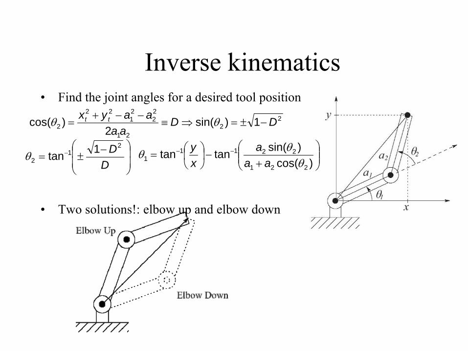
Inverse kinematics•
Find the joint angles for a desired tool position
•
Two solutions!: elbow up and elbow down
22
21
22
21
22
2 1)sin(2
)cos( DDaa
aayx tt −±=⇒≡−−+
= θθ
⎟⎟⎠
⎞⎜⎜⎝
⎛ −±= −
DD2
12
1tanθ ⎟⎟⎠
⎞⎜⎜⎝
⎛+
−⎟⎠⎞
⎜⎝⎛= −−
)cos()sin(tantan
221
22111 θ
θθaa
axy
•
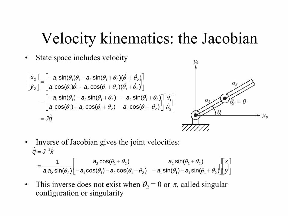
State space includes velocity
•
Inverse of Jacobian
gives the joint velocities:
•
This inverse does not exist when θ2 = 0 or π, called singular configuration or singularity
Velocity kinematics: the Jacobian
qJ
aaaaaa
aaaa
yx
&r
&
&
&&&
&&&
&
&
=
⎥⎦
⎤⎢⎣
⎡⎥⎦
⎤⎢⎣
⎡++++−+−−
=
⎥⎦
⎤⎢⎣
⎡
+++++−−
=⎥⎦
⎤⎢⎣
⎡
2
1
21221211
21221211
21212111
21212111
2
2
)cos()cos()cos()sin()sin()sin(
))(cos()cos())(sin()sin(
θθ
θθθθθθθθθθ
θθθθθθθθθθθθ
⎥⎦
⎤⎢⎣
⎡⎥⎦
⎤⎢⎣
⎡+−−+−−
++=
= −
yx
aaaaaa
aa
xJq
&
&
&r&r
)sin()sin()cos()cos()sin()cos(
)sin(1
2111121211
212212
221
1
θθθθθθθθθθ
θ

Problem: Lots of coordinate frames to calibrate
Robot–
Base frame–
End-effector
frame–
Object
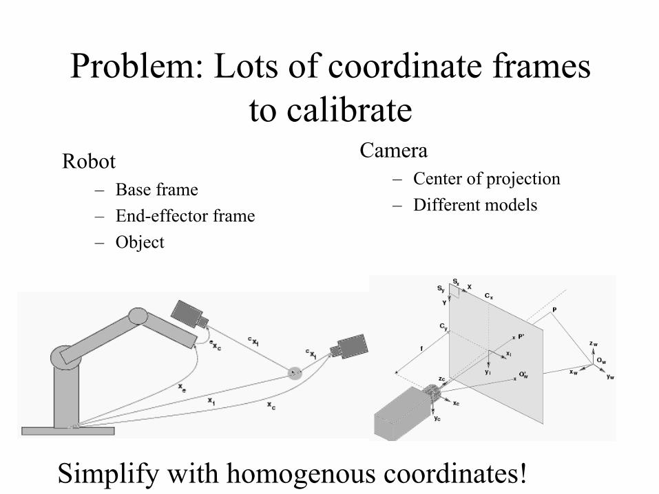
Problem: Lots of coordinate frames to calibrate
Camera–
Center of projection–
Different models
Robot–
Base frame–
End-effector
frame–
Object
Simplify with homogenous coordinates!
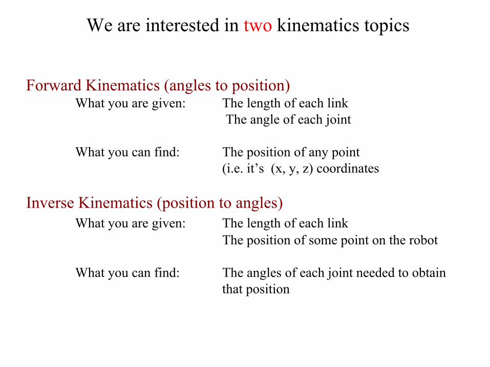
We are interested in two
kinematics topics
Forward Kinematics (angles to position)What you are given: The length of each link
The angle of each joint
What you can find: The position of any point(i.e. it’s (x, y, z) coordinates
Inverse Kinematics (position to angles)What you are given:
The length of each linkThe position of some point on the robot
What you can find:
The angles of each joint needed to obtain that position

X1
Y1
N
O
ΥVXY
X0
Y0
VNO
P
⎥⎦
⎤⎢⎣
⎡⎥⎦
⎤⎢⎣
⎡ −+⎥
⎦
⎤⎢⎣
⎡=⎥
⎦
⎤⎢⎣
⎡=
O
N
y
xY
XXY
VV
cos θsin θsin θcos θ
PP
VV
V
(VN,VO)
In other words, knowing the coordinates of a point (VN,VO) in some coordinate frame (NO) you can find the position of that point relative to your original coordinate frame (X0Y0).
(Note : Px
, Py
are relative to the original coordinate frame. Translation
followed by rotation
is different than rotation
followed by translation.)
Translation along P followed by rotation by θ
Change Coordinate Frame

⎥⎦
⎤⎢⎣
⎡⎥⎦
⎤⎢⎣
⎡ −+⎥
⎦
⎤⎢⎣
⎡=⎥
⎦
⎤⎢⎣
⎡=
O
N
y
xY
XXY
VV
cos θsin θsin θcos θ
PP
VV
V
HOMOGENEOUS REPRESENTATIONPutting it all into a Matrix
⎥⎥⎥
⎦
⎤
⎢⎢⎢
⎣
⎡
⎥⎥⎥
⎦
⎤
⎢⎢⎢
⎣
⎡ −+
⎥⎥⎥
⎦
⎤
⎢⎢⎢
⎣
⎡=
⎥⎥⎥
⎦
⎤
⎢⎢⎢
⎣
⎡
=1
VV
1000cos θsin θ0sin θcos θ
1PP
1VV
O
N
y
xY
X
⎥⎥⎥
⎦
⎤
⎢⎢⎢
⎣
⎡
⎥⎥⎥
⎦
⎤
⎢⎢⎢
⎣
⎡ −=
⎥⎥⎥
⎦
⎤
⎢⎢⎢
⎣
⎡
=1
VV
100Pcos θsin θPsin θcos θ
1VV
O
N
y
xY
X
What we found by doing a translation and a rotation
Padding with 0’s and 1’s
Simplifying into a matrix form
⎥⎥⎥
⎦
⎤
⎢⎢⎢
⎣
⎡ −=
100Pcos θsin θPsin θcos θ
H y
x
Homogenous Matrix for a Translation in XY plane, followed by a Rotation around the z-axis

Rotation Matrices in 3D –
OK,lets return from homogenous repn
⎥⎥⎥
⎦
⎤
⎢⎢⎢
⎣
⎡ −=
1000cos θsin θ0sin θcos θ
R z
⎥⎥⎥
⎦
⎤
⎢⎢⎢
⎣
⎡
−=
cos θ0sin θ010
sin θ0cos θR y
⎥⎥⎥
⎦
⎤
⎢⎢⎢
⎣
⎡−=cos θsin θ0sin θcos θ0001
R z
Rotation around the Z-Axis
Rotation around the Y-Axis
Rotation around the X-Axis

⎥⎥⎥⎥
⎦
⎤
⎢⎢⎢⎢
⎣
⎡
=
10000aon0aon0aon
Hzzz
yyy
xxx
Homogeneous Matrices in 3DH is a 4x4 matrix that can describe a translation, rotation, or both in one matrix
Translation without rotation⎥⎥⎥⎥
⎦
⎤
⎢⎢⎢⎢
⎣
⎡
=
1000P100P010P001
Hz
y
x
P
Y
X
Z
Y
X
Z
O
N
A
ON
ARotation without translation
Rotation part:Could be rotation around z-axis,
x-axis, y-axis or a combination of the three.

⎥⎥⎥⎥⎥
⎦
⎤
⎢⎢⎢⎢⎢
⎣
⎡
=
1
A
O
N
XY
VVV
HV
⎥⎥⎥⎥⎥
⎦
⎤
⎢⎢⎢⎢⎢
⎣
⎡
⎥⎥⎥⎥
⎦
⎤
⎢⎢⎢⎢
⎣
⎡
=
1
A
O
N
zzzz
yyyy
xxxx
XY
VVV
1000PaonPaonPaon
V
Homogeneous Continued….
The (n,o,a) position of a point relative to the current coordinate frame you are in.
The rotation and translation part can be combined into a single homogeneous matrix IF and ONLY IF both are relative to the same coordinate frame.
xA
xO
xN
xX PVaVoVnV +++=
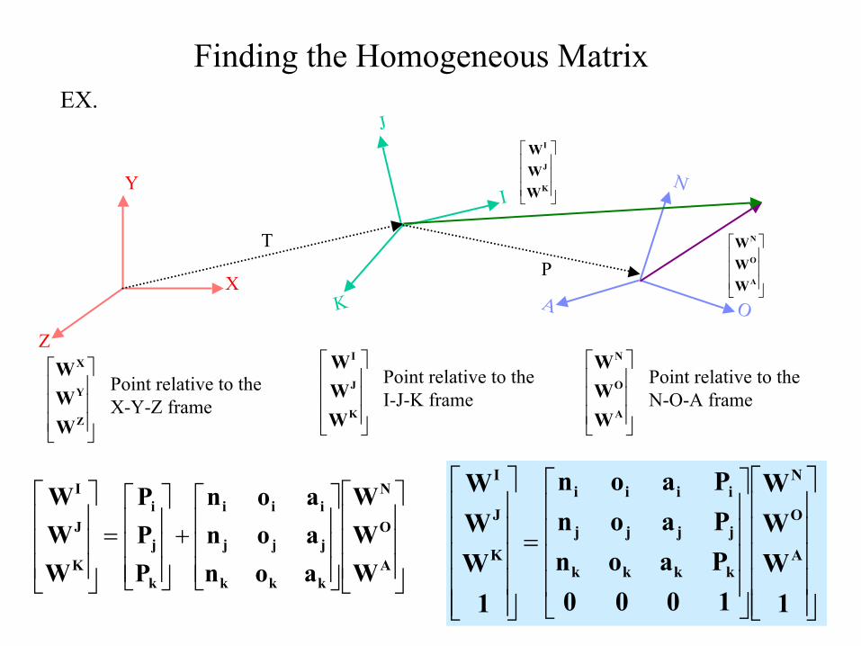
Finding the Homogeneous MatrixEX.
Y
X
Z
J
I
K
N
OA
TP
⎥⎥⎥
⎦
⎤
⎢⎢⎢
⎣
⎡
A
O
N
WWW
⎥⎥⎥
⎦
⎤
⎢⎢⎢
⎣
⎡
A
O
N
WWW
⎥⎥⎥
⎦
⎤
⎢⎢⎢
⎣
⎡
K
J
I
WWW
⎥⎥⎥
⎦
⎤
⎢⎢⎢
⎣
⎡
Z
Y
X
WWW Point relative to the
N-O-A framePoint relative to theX-Y-Z frame
Point relative to theI-J-K frame
⎥⎥⎥
⎦
⎤
⎢⎢⎢
⎣
⎡
⎥⎥⎥
⎦
⎤
⎢⎢⎢
⎣
⎡+
⎥⎥⎥
⎦
⎤
⎢⎢⎢
⎣
⎡=
⎥⎥⎥
⎦
⎤
⎢⎢⎢
⎣
⎡
A
O
N
kkk
jjj
iii
k
j
i
K
J
I
WWW
aonaonaon
PPP
WWW
⎥⎥⎥⎥⎥
⎦
⎤
⎢⎢⎢⎢⎢
⎣
⎡
⎥⎥⎥⎥
⎦
⎤
⎢⎢⎢⎢
⎣
⎡
=
⎥⎥⎥⎥⎥
⎦
⎤
⎢⎢⎢⎢⎢
⎣
⎡
1WWW
1000PaonPaonPaon
1WWW
A
O
N
kkkk
jjjj
iiii
K
J
I
⎥⎥⎥
⎦
⎤
⎢⎢⎢
⎣
⎡
K
J
I
WWW

Y
X
Z
J
I
K
N
OA
TP
⎥⎥⎥
⎦
⎤
⎢⎢⎢
⎣
⎡
A
O
N
WWW
⎥⎥⎥
⎦
⎤
⎢⎢⎢
⎣
⎡
⎥⎥⎥
⎦
⎤
⎢⎢⎢
⎣
⎡+
⎥⎥⎥
⎦
⎤
⎢⎢⎢
⎣
⎡=
⎥⎥⎥
⎦
⎤
⎢⎢⎢
⎣
⎡
k
J
I
zzz
yyy
xxx
z
y
x
Z
Y
X
WWW
kjikjikji
TTT
WWW
⎥⎥⎥⎥⎥
⎦
⎤
⎢⎢⎢⎢⎢
⎣
⎡
⎥⎥⎥⎥
⎦
⎤
⎢⎢⎢⎢
⎣
⎡
=
⎥⎥⎥⎥⎥
⎦
⎤
⎢⎢⎢⎢⎢
⎣
⎡
1WWW
1000TkjiTkjiTkji
1WWW
K
J
I
zzzz
yyyy
xxxx
Z
Y
X
Substituting for⎥⎥⎥
⎦
⎤
⎢⎢⎢
⎣
⎡
K
J
I
WWW
⎥⎥⎥⎥⎥
⎦
⎤
⎢⎢⎢⎢⎢
⎣
⎡
⎥⎥⎥⎥
⎦
⎤
⎢⎢⎢⎢
⎣
⎡
⎥⎥⎥⎥
⎦
⎤
⎢⎢⎢⎢
⎣
⎡
=
⎥⎥⎥⎥⎥
⎦
⎤
⎢⎢⎢⎢⎢
⎣
⎡
1WWW
1000PaonPaonPaon
1000TkjiTkjiTkji
1WWW
A
O
N
kkkk
jjjj
iiii
zzzz
yyyy
xxxx
Z
Y
X
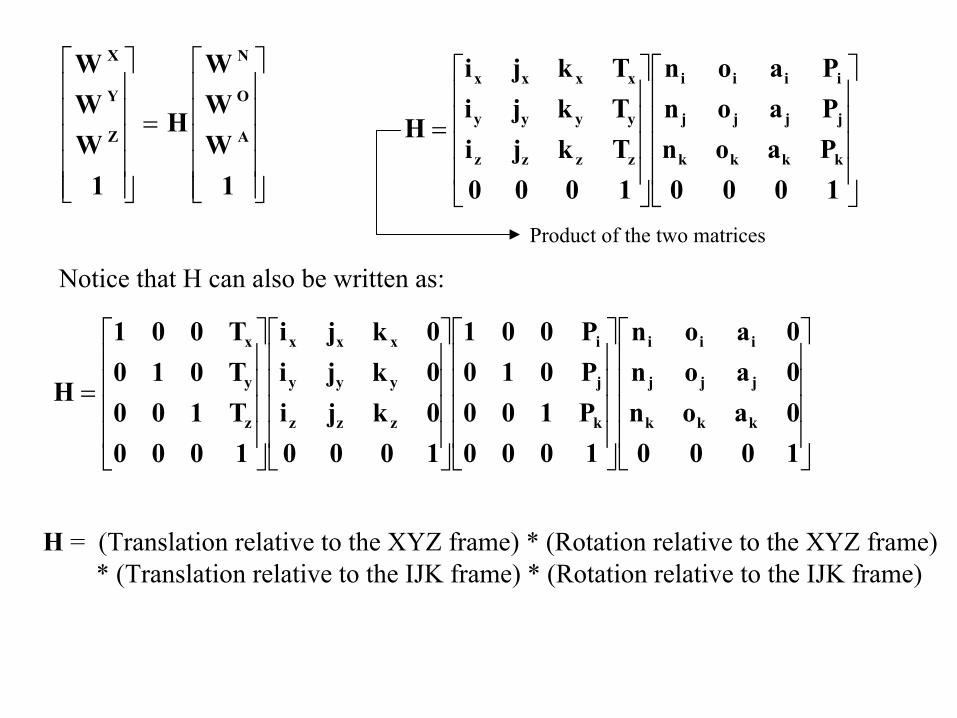
⎥⎥⎥⎥⎥
⎦
⎤
⎢⎢⎢⎢⎢
⎣
⎡
=
⎥⎥⎥⎥⎥
⎦
⎤
⎢⎢⎢⎢⎢
⎣
⎡
1WWW
H
1WWW
A
O
N
Z
Y
X
⎥⎥⎥⎥
⎦
⎤
⎢⎢⎢⎢
⎣
⎡
⎥⎥⎥⎥
⎦
⎤
⎢⎢⎢⎢
⎣
⎡
=
1000PaonPaonPaon
1000TkjiTkjiTkji
Hkkkk
jjjj
iiii
zzzz
yyyy
xxxx
Product of the two matrices
Notice that H can also be written as:
⎥⎥⎥⎥
⎦
⎤
⎢⎢⎢⎢
⎣
⎡
⎥⎥⎥⎥
⎦
⎤
⎢⎢⎢⎢
⎣
⎡
⎥⎥⎥⎥
⎦
⎤
⎢⎢⎢⎢
⎣
⎡
⎥⎥⎥⎥
⎦
⎤
⎢⎢⎢⎢
⎣
⎡
=
10000aon0aon0aon
1000P100P010P001
10000kji0kji0kji
1000T100T010T001
Hkkk
jjj
iii
k
j
i
zzz
yyy
xxx
z
y
x
H = (Translation relative to the XYZ frame) * (Rotation relative to the XYZ frame) * (Translation relative to the IJK frame) * (Rotation relative to the IJK frame)
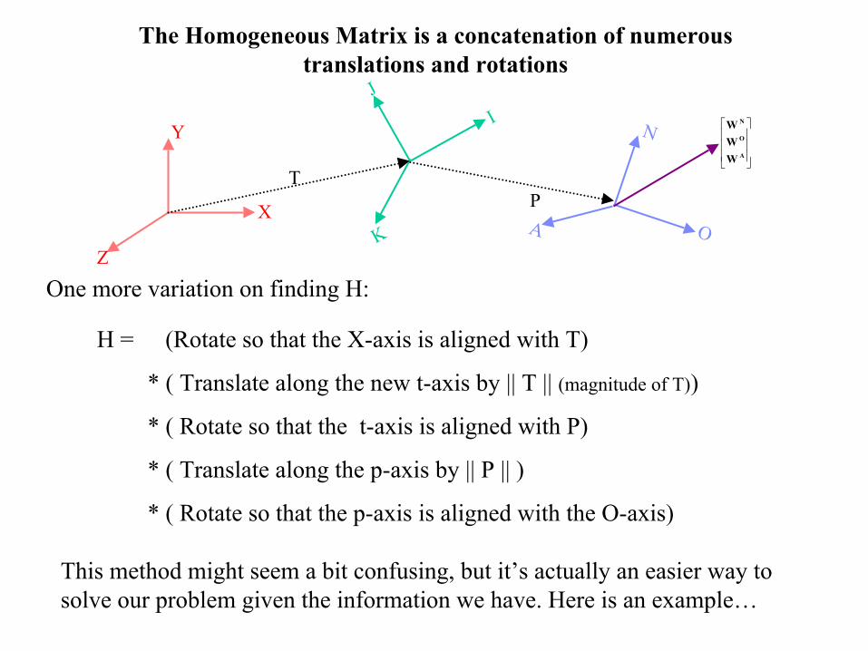
The Homogeneous Matrix is a concatenation of numerous translations and rotations
Y
X
Z
JI
K
N
OA
TP
⎥⎥⎥
⎦
⎤
⎢⎢⎢
⎣
⎡
A
O
N
WWW
One more variation on finding H:
H = (Rotate so that the X-axis is aligned with T)
* ( Translate along the new t-axis by || T || (magnitude of T))
* ( Rotate so that the t-axis is aligned with P)
* ( Translate along the p-axis by || P || )
* ( Rotate so that the p-axis is aligned with the O-axis)
This method might seem a bit confusing, but it’s actually an easier way to solve our problem given the information we have. Here is an example…
F o r w a r d K i n e m a t i c s
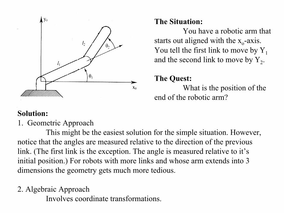
The Situation:You have a robotic arm that
starts out aligned with the xo
-axis.You tell the first link to move by Υ1
and the second link to move by Υ2
.
The Quest:What is the position of the
end of the robotic arm?
Solution:1. Geometric Approach
This might be the easiest solution for the simple situation. However, notice that the angles are measured relative to the direction of
the previous link. (The first link is the exception. The angle is measured relative to it’s initial position.) For robots with more links and whose arm extends into 3 dimensions the geometry gets much more tedious.
2. Algebraic Approach Involves coordinate transformations.

X2
X3Y2
Y3
Υ1
Υ2
Υ3
1
2 3
Example Problem: You are have a three link arm that starts out aligned in the x-axis.
Each link has lengths l1 , l2 , l3 , respectively. You tell the first one to move by Υ1
, and so on as the diagram suggests.
Find the Homogeneous matrix to get the position of the yellow dot in the X0Y0
frame.
H = Rz
(Υ1
) * Tx1
(l1 )
* Rz
(Υ2
) * Tx2
(l2 )
* Rz
(Υ3
)
i.e. Rotating by Υ1
will put you in the X1Y1
frame.Translate in the along the X1
axis by l1 .Rotating by Υ2
will put you in the X2Y2
frame.and so on until you are in the X3Y3
frame.
The position of the yellow dot relative to the X3Y3
frame
is(l1 , 0). Multiplying H by that position vector will give you the coordinates of the yellow point relative the the X0Y0
frame.
X1
Y1
X0
Y0

Slight variation on the last solution:Make the yellow dot the origin of a new coordinate X4Y4
frame
X2
X3Y2
Y3
Υ1
Υ2
Υ3
1
2 3
X1
Y1
X0
Y0
X4
Y4
H
=
Rz
(Υ1
) * Tx1
(l1 )
* Rz
(Υ2
) * Tx2
(l2 )
* Rz
(Υ3
) * Tx3
(l3 )
This takes you from the X0Y0
frame to the X4Y4
frame.
The position of the yellow dot relative to the X4Y4
frame is (0,0).
⎥⎥⎥⎥
⎦
⎤
⎢⎢⎢⎢
⎣
⎡
=
⎥⎥⎥⎥
⎦
⎤
⎢⎢⎢⎢
⎣
⎡
1000
H
1ZYX
Notice that multiplying by the (0,0,0,1) vector will equal the last column of the H matrix.

I n v e r s e K i n e m a t i c s
From Position to Angles

A Simple Example
Υ1
X
Y
S
Revolute and Prismatic Joints Combined
(x , y)
Finding Υ:
)xyarctan(θ =
More Specifically:
)xy(2arctanθ = arctan2() specifies that it’s in the
first quadrant
Finding S:
)y(xS 22+=
Υ2
Υ1
(x , y)
l2
l1
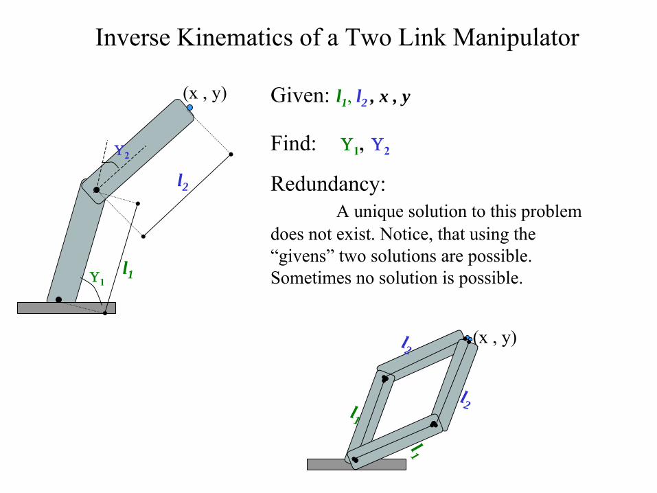
Inverse Kinematics of a Two Link Manipulator
Given:
l1 , l2 , x , y
Find: Υ1
, Υ2
Redundancy:A unique solution to this problem
does not exist. Notice, that using the “givens”
two solutions are possible. Sometimes no solution is possible.
(x , y)l2
l1l2
l1
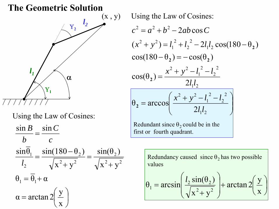
The Geometric Solution
l1
l2Υ2
Υ1
α
(x , y) Using the Law of Cosines:
⎟⎟⎠
⎞⎜⎜⎝
⎛ −−+=
−−+=
−=−−−+=+
−+=
21
22
21
22
21
22
21
22
212
22
122
222
2arccosθ
2)cos(θ
)cos(θ)θ180cos()θ180cos(2)(
cos2
llllyx
llllyx
llllyx
Cabbac
2
2
22
2
Using the Law of Cosines:
⎟⎠⎞
⎜⎝⎛=
+=
+=
+
−=
=
xy2arctanα
αθθ
yx)sin(θ
yx)θsin(180θsin
sinsin
11
222
222
2
1
l
cC
bB
⎟⎠⎞
⎜⎝⎛+
⎟⎟
⎠
⎞
⎜⎜
⎝
⎛
+=
xy2arctan
yx)sin(θarcsinθ
2222
1l
Redundant since θ2 could be in the first or fourth quadrant.
Redundancy caused since θ2 has two possible values

( ) ( )( )
⎟⎟⎠
⎞⎜⎜⎝
⎛ −−+=∴
++=
+++=
+++++=
=+=+
++
++++
21
22
21
22
2
2212
22
1
211211212
22
1
211212
212
22
12
1211212
212
22
12
1
2222
2yxarccosθ
c2
)(sins)(cc2
)(sins2)(sins)(cc2)(cc
yx)2((1)
llll
llll
llll
llllllll
The Algebraic Solution
l1
l2Υ2
Υ1
Υ(x , y)
21
21211
21211
1221
11
θθθ(3)sinsy(2)ccx(1)
)θcos( θccos θc
+=+=+=+=
=
+
+
+
llll
Only Unknown
))(sin(cos))(sin(cos)sin(
))(sin(sin))(cos(cos)cos(:
abbaba
bababaNote
+−
+−
−+
+−
=
=
X2
X3Y2
Y3
r1
r2
r3
1
2 3
X1
Y1
X0
Y0
X4
Y4
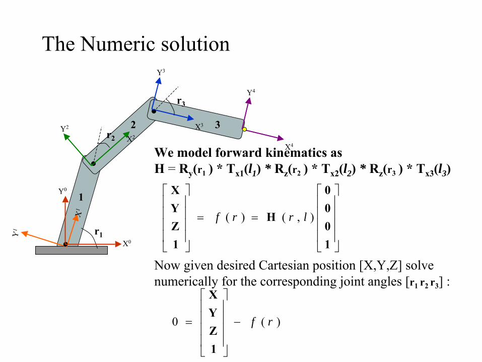
We model forward kinematics asH
= Ry
(r1
) * Tx1
(l1 )
* Rz
(r2
) * Tx2
(l2 )
* Rz
(r3
) * Tx3
(l3 )
Now given desired Cartesian position [X,Y,Z] solve numerically for the corresponding joint angles [r1 r2 r3
] :
⎥⎥⎥⎥
⎦
⎤
⎢⎢⎢⎢
⎣
⎡
==
⎥⎥⎥⎥
⎦
⎤
⎢⎢⎢⎢
⎣
⎡
1000
H
1ZYX
),()( lrrf
)(0 rf−
⎥⎥⎥⎥
⎦
⎤
⎢⎢⎢⎢
⎣
⎡
=
1ZYX
The Numeric solution

X2
X3Y2
Y3
r1
r2
r3
1
2 3
X1
Y1
X0
Y0
X4
Y4
Function:
Jacobian J = matrix of partial derivatives:
Newton’s method:Guess initial joint angles rIterate
J*dr = W-f( r )r = r+dr
If guess is close enough r converges to solution.Otherwise may diverge.
IlrrfW ),()(4 H==
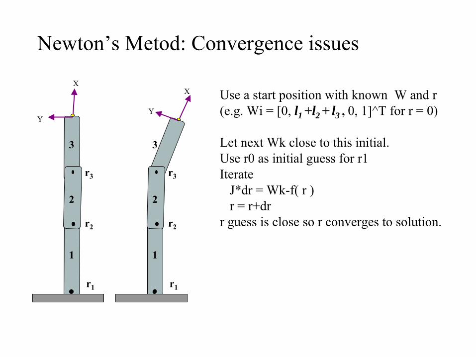
The Numeric solution: How to solve? Newton’s Metod
⎥⎥⎦
⎤
⎢⎢⎣
⎡
∂∂
=j
i
rrf )(J
r1
1
r2
2
r3
3
X
Y
Use a start position with known W and r(e.g. Wi
= [0, l1 +l2 + l3 , 0, 1]^T for r = 0)
Let next Wk close to this initial.Use r0 as initial guess for r1Iterate
J*dr = Wk-f( r )r = r+dr
r guess is close so r converges to solution.
Newton’s Metod: Convergence issues
r1
1
r2
2
r3
3
X
Y

r1
1
r2
2
r3
3
X
Y
To make a large movement, divide the total distance from (known) initial Wi to the new final Wf into small steps Wk e.g. on a line
•Try this in lab!
Newton’s Metod: Convergence issues
X3
r3
1
2 3
Y 1
X4
Y4
IlrrfW ),()(4 H==
⎥⎥⎦
⎤
⎢⎢⎣
⎡
∂∂
=j
i
rrf )(J

Resolved rate control
•
Here instead of computing an inverse kinematics solution then move the robot to that point, we actually move the robot dr for every iteration in newtons method.
•
Let dr 0, then we can view this as velocity control:
wtrr && 1))(( −= Jn velovitytranslatioCartesian == vw&

Conclusion•
Forward kinematics can be tedious for multilink arms
•
Inverse kinematics can be solved algebraically or numerically. The latter is more common for complex arms or vision-guided control (later)
•
Limitations: We avoided details of the various angular representations (Euler, quarternion or exponentials) and their detailed use in Kinematics. (this typically takes several weeks of course time in engineering courses)

Forward Kinematics (angles to position)What you are given: The length of each link
The angle of each joint
What you can find: The position of any point(i.e. it’s (x, y, z) coordinates
Inverse Kinematics (position to angles)What you are given:
The length of each linkThe position of some point on the robot
What you can find:
The angles of each joint needed to obtain that position
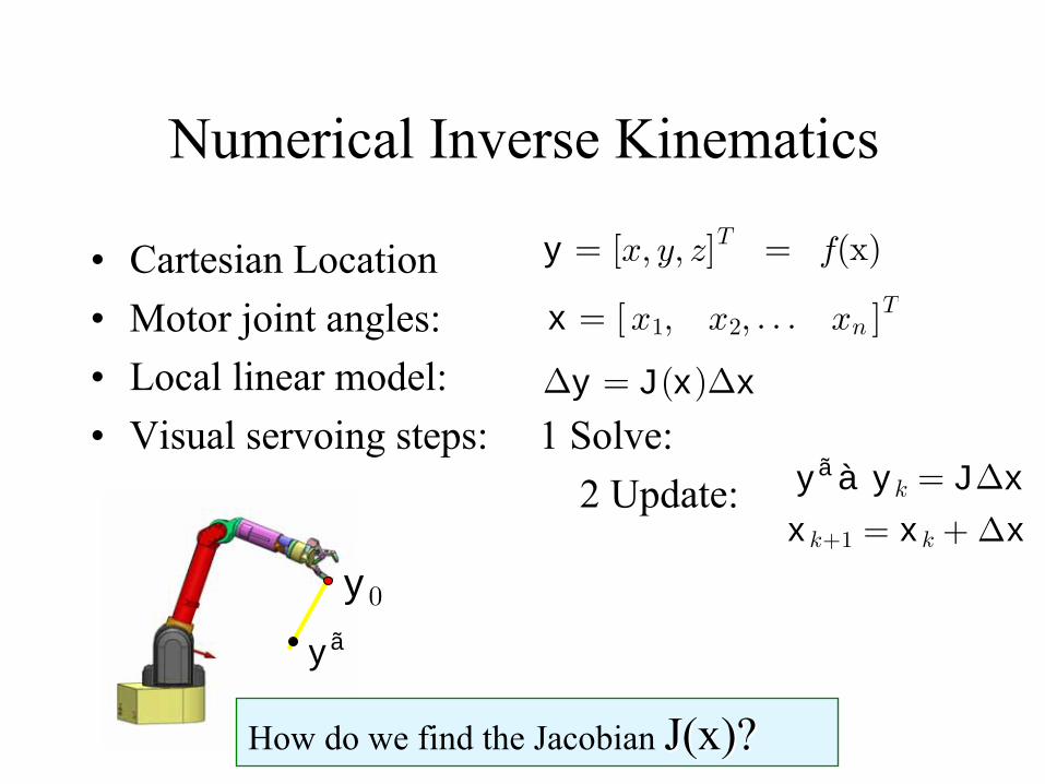
Lecture 2: Review Kinematics

Numerical Inverse Kinematics
•
Cartesian Location •
Motor joint angles:
•
Local linear model: •
Numerical steps: 1 Solve:
2 Update:
y = x, y, z[ ]T = f(x)
x = x1, x2, . . . xn[ ]T
Δy = J(x)Δx
yã à yk = JΔx
xk+1 = xk + Δx
y0
yã

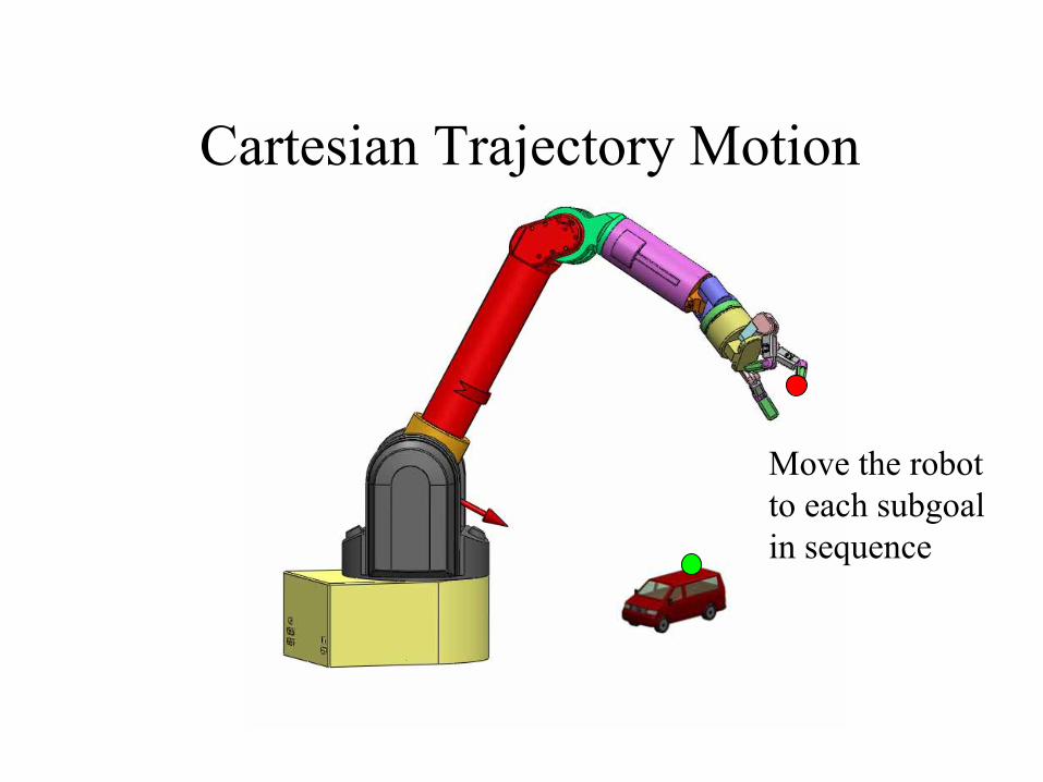
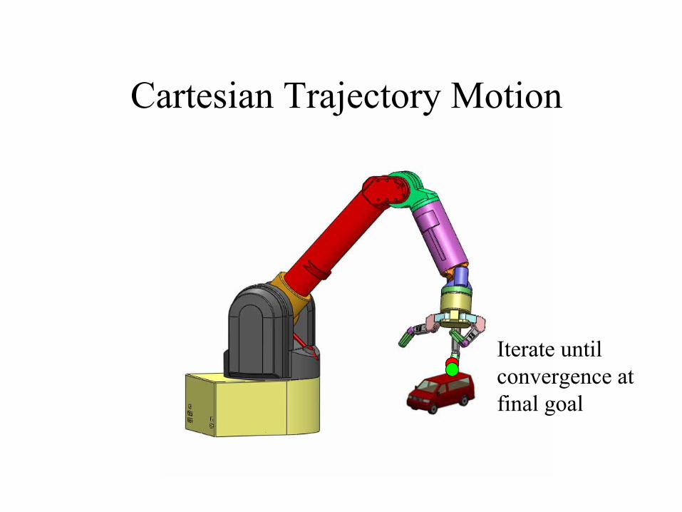
Cartesian Trajectory Motion
yã =xyz
" #Desired goal:
Current Cartesian positiony0

Cartesian Trajectory Motion
yã
Goal
Line with sub goals
y0
yk
y1
y2
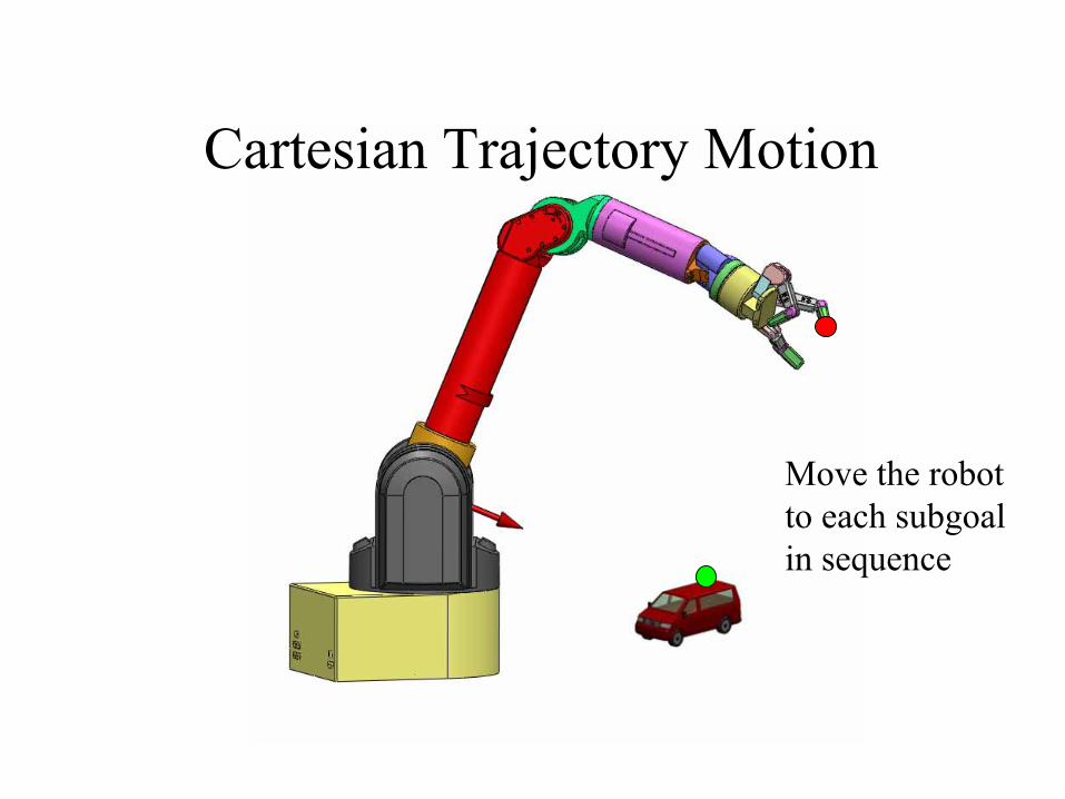
Cartesian Trajectory Motion
Move the robot to each subgoal in sequence
Cartesian Trajectory Motion
Move the robot to each subgoal in sequence

Cartesian Trajectory Motion
Move the robot to each subgoal in sequence
Cartesian Trajectory Motion
Iterate until convergence at final goal
Numerical Inverse Kinematics
•
Cartesian Location •
Motor joint angles:
•
Local linear model: •
Visual servoing steps: 1 Solve:
2 Update:
y = x, y, z[ ]T = f(x)
x = x1, x2, . . . xn[ ]T
Δy = J(x)Δx
yã à yk = JΔx
xk+1 = xk + Δx
y0
yã
How do we find the Jacobian J(x)?J(x)?
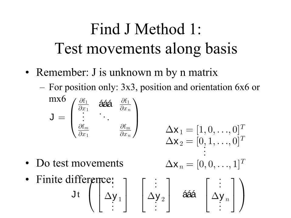
Find J Method 1: Test movements along basis
•
Remember: J is unknown m by n matrix–
For position only: 3x3, position and orientation 6x6 or mx6
•
Do test movements •
Finite difference:
J =∂x1
∂f1 á á á∂xn
∂f1
.... . .
∂x1
∂fm∂xn
∂fm
⎛⎜⎝⎞⎟⎠
Δx1 = [1, 0, . . ., 0]T
Δx2 = [0, 1, . . ., 0]T...Δxn = [0, 0, . . ., 1]T
Jt
...Δy1...
⎡⎣ ⎤⎦ ...Δy2...
⎡⎣ ⎤⎦ á á á
...Δyn...
⎡⎣ ⎤⎦⎛⎝ ⎞⎠

Find J Method 2: Secant Constraints
•
Constraint along a line:•
Defines m equations
•
Collect n arbitrary, but different measures
y•
Solve for J
Δy = JΔx
á á á ΔyT1 á á á
á á á ΔyT2 á á á
â ã...
á á á ΔyTn á á á
â ã⎛⎜⎜⎝
⎞⎟⎟⎠ =
á á á ΔxT1 á á á
á á á ΔxT2 á á á
â ã...
á á á ΔxTn á á á
â ã⎛⎜⎜⎝
⎞⎟⎟⎠ JT

Find J Method 3: Recursive Secant Constraints
Broydens method•
Based on initial J and one measure pair
•
Adjust J s.t. •
Rank 1 update:
•
Consider rotated coordinates: –
Update same as finite difference for n
orthogonal
moves
Δy,Δx
Δy = Jk+1Δx
Jêk+1 = Jêk +ΔxTΔx
(Δy à JêkΔx)ΔxT
Δx
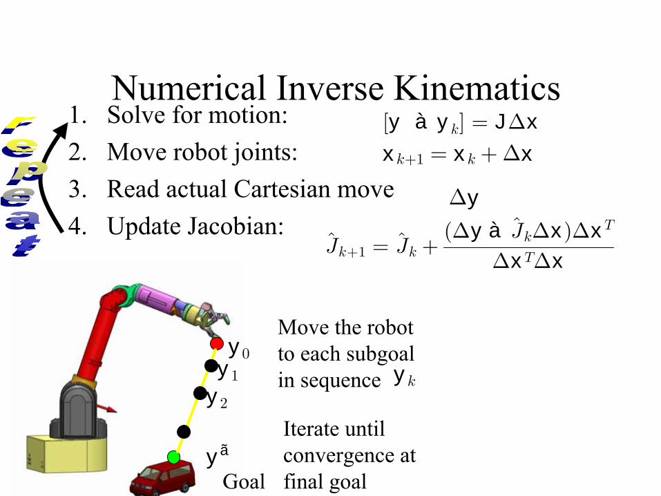
Numerical Inverse Kinematics 1.
Solve for motion:
2.
Move robot joints:3.
Read actual Cartesian move
4.
Update Jacobian:
[y à yk] = JΔx
xk+1 = xk +Δx
Jêk+1 = Jêk +ΔxTΔx
(Δy à JêkΔx)ΔxT
Δy
Move the robot to each subgoal in sequence
yã
Goal
y0
yky1
y2
Δy
Iterate until convergence at final goal

Singularities
•
J singular cannot solve eqs•
Definition: we say that any configuration in which the rank of J is less than its maximum is a singular configuration–
i.e. any configuration that causes J to lose rank is a singular configuration
•
Characteristics of singularities:–
At a singularity, motion in some directions will not be possible
–
At and near singularities, bounded end effector
velocities would require unbounded joint velocities
–
At and near singularities, bounded joint torques may produce unbounded end effector
forces and torques–
Singularities often occur along the workspace boundary (i.e. when the arm is fully extended)
[y à yk] = JΔx
Singularities
•
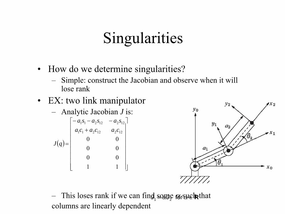
How do we determine singularities?–
Simple: construct the Jacobian
and observe when it will lose rank
•
EX: two link manipulator–
Analytic Jacobian
J is:
–
This loses rank if we can find some α such thatcolumns are linearly dependent
( )
⎥⎥⎥⎥⎥⎥⎥⎥
⎦
⎤
⎢⎢⎢⎢⎢⎢⎢⎢
⎣
⎡+
−−−
=
11000000
12212211
12212211
cacacasasasa
qJ
R∈= αα for 21 JJ
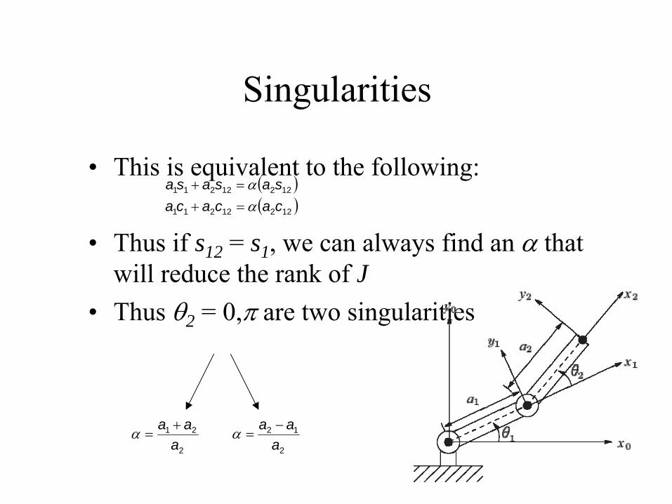
Singularities
•
This is equivalent to the following:
•
Thus if s12 = s1 , we can always find an α that will reduce the rank of J
•
Thus θ2 = 0,π are two singularities
( )( )12212211
12212211
cacacasasasa
αα
=+=+
2
21
aaa +
=α2
12
aaa −
=α

Determining Singular Configurations
•
In general, all we need to do is observe how the rank of the Jacobian
changes as the configuration
changes•
Can study analytically
•
Or numerically: Singular if eigenvalues of square matrix 0, or singular values of rectangular matrix zero. (Compute with SVD), or condition number tends to infinity.
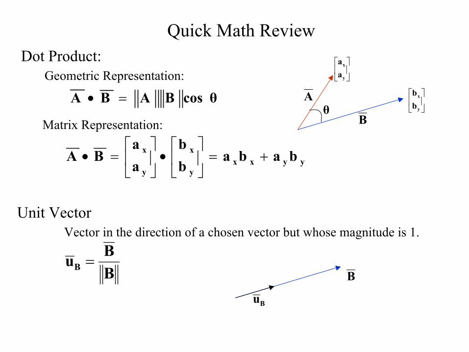
Quick Math ReviewDot Product:
Geometric Representation:A
Bθ
cos θBABA =•
Unit VectorVector in the direction of a chosen vector but whose magnitude is 1.
BBuB =
⎥⎦
⎤⎢⎣
⎡
y
x
aa
⎥⎦
⎤⎢⎣
⎡
y
x
bb
Matrix Representation:
yyxxy
x
y
x bababb
aa
BA +=⎥⎦
⎤⎢⎣
⎡•⎥
⎦
⎤⎢⎣
⎡=•
B
Bu

Quick Matrix Review
Matrix Multiplication:
An (m x n) matrix A and an (n x p) matrix B, can be multiplied since the number of columns of A is equal to the number of rows of B.
Non-Commutative MultiplicationAB is NOT
equal to BA
( ) ( )( ) ( )⎥⎦
⎤⎢⎣
⎡++++
=⎥⎦
⎤⎢⎣
⎡∗⎥⎦
⎤⎢⎣
⎡dhcfdgcebhafbgae
hgfe
dcba
Matrix Addition:( ) ( )( ) ( )⎥⎦
⎤⎢⎣
⎡++++
=⎥⎦
⎤⎢⎣
⎡+⎥
⎦
⎤⎢⎣
⎡hdgcfbea
hgfe
dcba

Basic TransformationsMoving Between Coordinate Frames
Translation Along the X-Axis
N
O
X
Y
VNO
VXY
Px
VN
VO
Px
= distance between the XY and NO coordinate planes
⎥⎦
⎤⎢⎣
⎡=
Y
XXY
VV
V ⎥⎦
⎤⎢⎣
⎡=
O
NNO
VV
V ⎥⎦
⎤⎢⎣
⎡=
0P
P x
P
(VN,VO)
Notation:
NX
VNO
VXY
PVN
VO
Y O
Υ
NOO
NXXY VPV
VPV +=⎥
⎦
⎤⎢⎣
⎡ +=
Writing in terms of XYV NOV

X
VXY
PXY
N
VNO
VN
VO
O
Y
Translation along the X-Axis and Y-Axis
⎥⎦
⎤⎢⎣
⎡
++
=+= OY
NXNOXY
VPVP
VPV
⎥⎦
⎤⎢⎣
⎡=
Y
xXY
PP
P

⎥⎦
⎤⎢⎣
⎡
••
=⎥⎥⎦
⎤
⎢⎢⎣
⎡
−=
⎥⎥⎦
⎤
⎢⎢⎣
⎡=⎥
⎦
⎤⎢⎣
⎡=
oVnV
θ)cos(90VcosθV
sinθVcosθV
VV
V NO
NO
NO
NO
NO
NO
O
NNO
NOV
on Unit vector along the N-Axis
Unit vector along the N-Axis
Magnitude of the VNO vector
Using Basis VectorsBasis vectors are unit vectors that point along a coordinate axis
N
VNO
VN
VO
O
n
o
Rotation (around the Z-Axis)X
Y
Z
X
Y
N
VN
VO
O
Υ
V
VX
VY
⎥⎦
⎤⎢⎣
⎡=
Y
XXY
VV
V ⎥⎦
⎤⎢⎣
⎡=
O
NNO
VV
V
Υ
= Angle of rotation between the XY and NO coordinate axis

X
Y
N
VN
VO
O
Υ
V
VX
VY
α
Unit vector along X-Axisx
xVcos αVcos αVV NONOXYX •===
NOXY VV =
Can be considered with respect to the XY coordinates or NO coordinatesV
x)oVn(VV ONX •∗+∗= (Substituting for VNO
using the N and O components of the vector)
)oxVnxVV ONX •+•= ()(
)))
(sin θV(cos θV90))(cos( θV(cos θV
ON
ON
−=
++=

Similarly….
yVα)cos(90Vsin αVV NONONOY •=−==
y)oVn(VV ONY •∗+∗=
)oy(V)ny(VV ONY •+•=
)))
(cos θV(sin θV(cos θVθ))(cos(90V
ON
ON
+=
+−=
So….
)) (cos θV(sin θVV ONY +=)) (sin θV(cos θVV ONX −= ⎥
⎦
⎤⎢⎣
⎡=
Y
XXY
VV
V
Written in Matrix Form
⎥⎦
⎤⎢⎣
⎡⎥⎦
⎤⎢⎣
⎡ −=⎥
⎦
⎤⎢⎣
⎡=
O
N
Y
XXY
VV
cosθsinθsinθcosθ
VV
V Rotation Matrix about the z-axis
))(sin(cos))(sin(cos)sin(
))(sin(sin))(cos(cos)cos(:
abbaba
bababaNote
+−
+−
−+
+−
=
=
)c(s)s(c cscss
sinsy
)()c(c ccc
ccx
2211221
12221211
21211
2212211
21221211
21211
llllll
ll
slsllsslll
ll
++=++=
+=
−+=−+=
+=
+
+
We know what θ2
is from the previous slide. We need to solve for θ1
. Now we have two equations and two unknowns (sin θ1
and cos
θ1
)
( )
2222221
1
2212
22
1122221
221122221
221
221
2211
yxx)c(ys
)c2(sx)c(
1
)c(s)s()c()(xy
)c()(xc
+
−+=
++++
=
+++
+=
++
=
slll
llllslll
lllll
slsll
sls
Substituting for c1
and simplifying many times
Notice this is the law of cosines and can be replaced by x2+ y2
⎟⎟⎠
⎞⎜⎜⎝
⎛
+
−+= 22
222211 yx
x)c(yarcsinθ slll