coastwatch software library and utilities user’s guide
TRANSCRIPT

CoastWatch Software Library andUtilities User’s Guide
Version 3.2.3Revised April 1, 2009
Prepared by:Peter Hollemans
Terrenus Earth Sciences, Consultant for NOAA/NESDIS
U.S. DEPARTMENT OF COMMERCENATIONAL OCEANIC AND ATMOSPHERIC ADMINISTRATION
NATIONAL ENVIRONMENTAL SATELLITE, DATA, AND INFORMATION SERVICE
COASTWATCH PROGRAM

i
Copyright Notice
CoastWatch Software Library and UtilitiesCopyright 1998-2009, USDOC/NOAA/NESDIS CoastWatch
Permission to use, copy, modify, and distribute this software and its documentation for any purposeand without fee is hereby granted, provided that the above copyright notice appear in all copies, thatboth the copyright notice and this permission notice appear in supporting documentation, and thatredistributions of modified forms of the source or binary code carry prominent notices stating that theoriginal code was changed and the date of the change. This software is provided “as is” without expressor implied warranty.
Privacy Policy
On startup, this software queries network servers for up-to-date version information, at which timedata is collected and stored by the server automatically concerning the computer IP address, type ofoperating system, version of the software, and the date and time. This information does not identifyyou personally. It is used to help improve the software by providing usage statistics. More details onNOAA’s privacy policy may be found at http://www.noaa.gov/privacy.html.
Obtaining a Copy
To download a copy of the CoastWatch Utilities, visit:
http://coastwatch.noaa.gov/cw cwfv3.html
For general information on CoastWatch products and services, visit:
http://coastwatch.noaa.gov
Providing Feedback
Email questions, comments, suggestions, and bug reports to the CoastWatch help desk [email protected]. In order to receive help, you should include the following information:
1. The version and operating system of the software, for example cwf-3.2.1 on Windows XP.
2. The type of data file and where you obtained the file, for example CoastWatch .cwf files obtainedfrom the SAA web site. If the data origin is unknown, include some example data filenames.
3. If sending a bug report or asking for clarification, a description of how to reproduce your result:
• For a command-line tool, a transcript of the terminal session during which the question orproblem arose. You can cut and paste the contents of the terminal session including thecommand used and its output directly into the email.

ii
• For a graphical interface tool, a list of steps to reproduce the problem. For example, Opendata file xxx, click this button, then that button.

Contents
Preface 1
1 Introduction 3
1.1 A Brief History . . . . . . . . . . . . . . . . . . . . . . . . . . . . . . . . . . . . . . . . . 3
1.2 Installation Notes . . . . . . . . . . . . . . . . . . . . . . . . . . . . . . . . . . . . . . . . 4
1.2.1 System Requirements . . . . . . . . . . . . . . . . . . . . . . . . . . . . . . . . . 4
1.2.2 Downloading . . . . . . . . . . . . . . . . . . . . . . . . . . . . . . . . . . . . . . 4
1.2.3 Installing on Windows . . . . . . . . . . . . . . . . . . . . . . . . . . . . . . . . . 4
1.2.4 Installing on Mac OS X . . . . . . . . . . . . . . . . . . . . . . . . . . . . . . . . 5
1.2.5 Installing on Unix . . . . . . . . . . . . . . . . . . . . . . . . . . . . . . . . . . . 5
1.3 Using the Software . . . . . . . . . . . . . . . . . . . . . . . . . . . . . . . . . . . . . . . 5
1.4 Third Party Software . . . . . . . . . . . . . . . . . . . . . . . . . . . . . . . . . . . . . . 6
2 Common Tasks 7
2.1 Information and Statistics . . . . . . . . . . . . . . . . . . . . . . . . . . . . . . . . . . . 7
2.2 Data Processing . . . . . . . . . . . . . . . . . . . . . . . . . . . . . . . . . . . . . . . . 8
2.3 Graphics and Visualization . . . . . . . . . . . . . . . . . . . . . . . . . . . . . . . . . . 8
2.4 Registration and Navigation . . . . . . . . . . . . . . . . . . . . . . . . . . . . . . . . . . 9
2.5 Network . . . . . . . . . . . . . . . . . . . . . . . . . . . . . . . . . . . . . . . . . . . . . 10
3 The CoastWatch Data Analysis Tool 11
3.1 Getting to know CDAT . . . . . . . . . . . . . . . . . . . . . . . . . . . . . . . . . . . . 11
3.2 Loading data files . . . . . . . . . . . . . . . . . . . . . . . . . . . . . . . . . . . . . . . . 13
3.3 Navigating in CDAT . . . . . . . . . . . . . . . . . . . . . . . . . . . . . . . . . . . . . . 14
3.4 Changing data image colors . . . . . . . . . . . . . . . . . . . . . . . . . . . . . . . . . . 14
iii

iv CONTENTS
3.5 Displaying coastlines, grids, and more . . . . . . . . . . . . . . . . . . . . . . . . . . . . 15
3.5.1 Types of overlays . . . . . . . . . . . . . . . . . . . . . . . . . . . . . . . . . . . . 16
3.5.2 The Overlay List . . . . . . . . . . . . . . . . . . . . . . . . . . . . . . . . . . . . 18
3.5.3 Overlay groups . . . . . . . . . . . . . . . . . . . . . . . . . . . . . . . . . . . . . 19
3.6 Measuring distances and data statistics . . . . . . . . . . . . . . . . . . . . . . . . . . . 20
3.6.1 Types of surveys . . . . . . . . . . . . . . . . . . . . . . . . . . . . . . . . . . . . 20
3.6.2 The Survey List and results . . . . . . . . . . . . . . . . . . . . . . . . . . . . . . 21
3.7 Drawing lines, shapes, and text . . . . . . . . . . . . . . . . . . . . . . . . . . . . . . . . 21
3.7.1 Types of annotations . . . . . . . . . . . . . . . . . . . . . . . . . . . . . . . . . . 21
3.7.2 The Annotation List . . . . . . . . . . . . . . . . . . . . . . . . . . . . . . . . . . 22
3.8 Using composite image mode . . . . . . . . . . . . . . . . . . . . . . . . . . . . . . . . . 23
3.9 Correcting geographic location problems . . . . . . . . . . . . . . . . . . . . . . . . . . . 23
3.9.1 Navigation correction . . . . . . . . . . . . . . . . . . . . . . . . . . . . . . . . . 25
3.9.2 Navigation analysis . . . . . . . . . . . . . . . . . . . . . . . . . . . . . . . . . . . 26
3.10 Exporting images and data . . . . . . . . . . . . . . . . . . . . . . . . . . . . . . . . . . 28
3.11 Setting color, enhancement, and units preferences . . . . . . . . . . . . . . . . . . . . . . 29
3.11.1 Resources directory . . . . . . . . . . . . . . . . . . . . . . . . . . . . . . . . . . 31
3.12 Connections with command line tools . . . . . . . . . . . . . . . . . . . . . . . . . . . . 32
4 Programmer’s API 35
4.1 How to use the API . . . . . . . . . . . . . . . . . . . . . . . . . . . . . . . . . . . . . . 35
4.2 Data I/O . . . . . . . . . . . . . . . . . . . . . . . . . . . . . . . . . . . . . . . . . . . . 37
4.3 Data rendering . . . . . . . . . . . . . . . . . . . . . . . . . . . . . . . . . . . . . . . . . 38
4.4 Graphical user interface components . . . . . . . . . . . . . . . . . . . . . . . . . . . . . 39
4.5 General utility classes . . . . . . . . . . . . . . . . . . . . . . . . . . . . . . . . . . . . . 40
4.6 Main programs . . . . . . . . . . . . . . . . . . . . . . . . . . . . . . . . . . . . . . . . . 41
A Manual Pages 43
A.1 cdat . . . . . . . . . . . . . . . . . . . . . . . . . . . . . . . . . . . . . . . . . . . . . . . 43
A.2 cwangles . . . . . . . . . . . . . . . . . . . . . . . . . . . . . . . . . . . . . . . . . . . . . 45
A.3 cwautonav . . . . . . . . . . . . . . . . . . . . . . . . . . . . . . . . . . . . . . . . . . . . 48
A.4 cwcomposite . . . . . . . . . . . . . . . . . . . . . . . . . . . . . . . . . . . . . . . . . . . 57
A.5 cwcoverage . . . . . . . . . . . . . . . . . . . . . . . . . . . . . . . . . . . . . . . . . . . 60

CONTENTS v
A.6 cwdownload . . . . . . . . . . . . . . . . . . . . . . . . . . . . . . . . . . . . . . . . . . . 64
A.7 cwexport . . . . . . . . . . . . . . . . . . . . . . . . . . . . . . . . . . . . . . . . . . . . . 67
A.8 cwgraphics . . . . . . . . . . . . . . . . . . . . . . . . . . . . . . . . . . . . . . . . . . . 73
A.9 cwimport . . . . . . . . . . . . . . . . . . . . . . . . . . . . . . . . . . . . . . . . . . . . 76
A.10 cwinfo . . . . . . . . . . . . . . . . . . . . . . . . . . . . . . . . . . . . . . . . . . . . . . 78
A.11 cwmaster . . . . . . . . . . . . . . . . . . . . . . . . . . . . . . . . . . . . . . . . . . . . 81
A.12 cwmath . . . . . . . . . . . . . . . . . . . . . . . . . . . . . . . . . . . . . . . . . . . . . 83
A.13 cwnavigate . . . . . . . . . . . . . . . . . . . . . . . . . . . . . . . . . . . . . . . . . . . 89
A.14 cwregister . . . . . . . . . . . . . . . . . . . . . . . . . . . . . . . . . . . . . . . . . . . . 93
A.15 cwrender . . . . . . . . . . . . . . . . . . . . . . . . . . . . . . . . . . . . . . . . . . . . . 96
A.16 cwsample . . . . . . . . . . . . . . . . . . . . . . . . . . . . . . . . . . . . . . . . . . . . 108
A.17 cwstats . . . . . . . . . . . . . . . . . . . . . . . . . . . . . . . . . . . . . . . . . . . . . 112
A.18 cwstatus . . . . . . . . . . . . . . . . . . . . . . . . . . . . . . . . . . . . . . . . . . . . . 115
A.19 hdatt . . . . . . . . . . . . . . . . . . . . . . . . . . . . . . . . . . . . . . . . . . . . . . . 117
B CoastWatch HDF Metadata Specification 121
B.1 Overview . . . . . . . . . . . . . . . . . . . . . . . . . . . . . . . . . . . . . . . . . . . . 121
B.2 Global Metadata . . . . . . . . . . . . . . . . . . . . . . . . . . . . . . . . . . . . . . . . 122
B.3 Earth Location Metadata . . . . . . . . . . . . . . . . . . . . . . . . . . . . . . . . . . . 123
B.3.1 Version 2 Affine . . . . . . . . . . . . . . . . . . . . . . . . . . . . . . . . . . . . . 125
B.3.2 Version 3 Affine . . . . . . . . . . . . . . . . . . . . . . . . . . . . . . . . . . . . . 126
B.4 Variable Metadata . . . . . . . . . . . . . . . . . . . . . . . . . . . . . . . . . . . . . . . 126
B.4.1 Calibration Values . . . . . . . . . . . . . . . . . . . . . . . . . . . . . . . . . . . 128
B.4.2 Navigation Correction . . . . . . . . . . . . . . . . . . . . . . . . . . . . . . . . . 128
B.5 Swath Earth Location Encoding . . . . . . . . . . . . . . . . . . . . . . . . . . . . . . . 129
B.6 GCTP Appendices . . . . . . . . . . . . . . . . . . . . . . . . . . . . . . . . . . . . . . . 134
C Data Format Compatibility 149
D Miscellaneous Formats 151
D.1 Navigation analysis XML output . . . . . . . . . . . . . . . . . . . . . . . . . . . . . . . 151
D.2 Navigation analysis CSV output . . . . . . . . . . . . . . . . . . . . . . . . . . . . . . . 153
D.3 Color palette XML format . . . . . . . . . . . . . . . . . . . . . . . . . . . . . . . . . . . 153

vi CONTENTS
E AVHRR SST Product FAQ 155
E.1 Data formats and archiving . . . . . . . . . . . . . . . . . . . . . . . . . . . . . . . . . . 155
E.2 SST computation . . . . . . . . . . . . . . . . . . . . . . . . . . . . . . . . . . . . . . . . 157
E.3 Cloud masking . . . . . . . . . . . . . . . . . . . . . . . . . . . . . . . . . . . . . . . . . 158
E.4 Navigation correction . . . . . . . . . . . . . . . . . . . . . . . . . . . . . . . . . . . . . 160
E.5 Map projections . . . . . . . . . . . . . . . . . . . . . . . . . . . . . . . . . . . . . . . . 162
F Acronyms 165
G History of Changes 167

List of Figures
3.1 Components of the CDAT window . . . . . . . . . . . . . . . . . . . . . . . . . . . . . . 12
3.2 File Open window . . . . . . . . . . . . . . . . . . . . . . . . . . . . . . . . . . . . . . . 13
3.3 Color conversion tabs . . . . . . . . . . . . . . . . . . . . . . . . . . . . . . . . . . . . . 15
3.4 Color enhancement process . . . . . . . . . . . . . . . . . . . . . . . . . . . . . . . . . . 16
3.5 Overlay graphics drawing order . . . . . . . . . . . . . . . . . . . . . . . . . . . . . . . . 17
3.6 Overlay Layers tab . . . . . . . . . . . . . . . . . . . . . . . . . . . . . . . . . . . . . . . 17
3.7 Examples of default overlay groups . . . . . . . . . . . . . . . . . . . . . . . . . . . . . . 19
3.8 Data Surveys tab . . . . . . . . . . . . . . . . . . . . . . . . . . . . . . . . . . . . . . . . 20
3.9 Annotations tab . . . . . . . . . . . . . . . . . . . . . . . . . . . . . . . . . . . . . . . . 22
3.10 Color Composite tab . . . . . . . . . . . . . . . . . . . . . . . . . . . . . . . . . . . . . . 23
3.11 RGB composite examples . . . . . . . . . . . . . . . . . . . . . . . . . . . . . . . . . . . 24
3.12 Navigation Correction tab . . . . . . . . . . . . . . . . . . . . . . . . . . . . . . . . . . . 25
3.13 Navigation correction example . . . . . . . . . . . . . . . . . . . . . . . . . . . . . . . . 26
3.14 Navigation Analysis panel . . . . . . . . . . . . . . . . . . . . . . . . . . . . . . . . . . . 27
3.15 Enhancement section in the Preferences panel . . . . . . . . . . . . . . . . . . . . . . . . 30
B.1 A partitioning of AVHRR swath data . . . . . . . . . . . . . . . . . . . . . . . . . . . . 130
B.2 Sampling pattern for polynomial approximation . . . . . . . . . . . . . . . . . . . . . . . 131
B.3 Binary tree encoding example . . . . . . . . . . . . . . . . . . . . . . . . . . . . . . . . . 132
B.4 A more complex binary tree encoding example . . . . . . . . . . . . . . . . . . . . . . . 132
vii

Preface
Typographic Conventions
In this manual, we use the following conventions for the font and color of text. References within thedocument are in the standard font, but are red to emphasize that they are active links, for example areference to a section: “see chapter 3 for information on the CoastWatch Data Analaysis Tool”. Externalreferences are a typewriter font in magenta, such as a web site address: “http://www.google.comis a great search engine”. Terminal commands, terminal output, file names, and verbatim characterstrings are in a typewriter font. Java class names are in italics. Replacement parameters in commandline programs are in CAPITALS.
Acknowledgments
We would like to acknowledge the following parties for support in creating the CoastWatch Utilitiessoftware (in no particular order):
• John Sapper of NOAA/NESDIS, CoastWatch central operations, and many other NOAA/NESDISresearchers for continued funding support and new requirements.
• The CoastWatch node managers, operations managers, and CLASS archive staff who were invalu-able in providing feedback.
• CoastWatch data users who have provided critical review of the software, bug reports, and newideas for functionality.
• The open source software community for providing high quality code libraries upon which theutilities are built.
1

2 LIST OF FIGURES
Chapter 1
Introduction
The main goal of the CoastWatch Utilities software is to aid data users in working with NOAA/NESDISCoastWatch satellite data. CoastWatch data is distributed as individual files in a scientific data formatthat is not recognized by standard image viewers, and the CoastWatch Utilities are useful for manipu-lating data and creating images from CoastWatch data for both recreational and scientific applications.CoastWatch data files contain:
1. Global file attributes that describe the date/time and location of the earth data in the file, as wellas any relevant data processing details.
2. Earth data as a set of two-dimensional numerical arrays, each with a unique name. These variableshold the actual scientific data and accompanying attributes, such as scaling factor and units, thatdescribe how to use the data values.
The CoastWatch Utilities allow users to selectively access and extract this information in a number ofways.
1.1 A Brief History
The CoastWatch Utilities have been evolving since 1998. The original software was capable of workingwith CoastWatch IMGMAP format data files, the standard data distribution format (limited to NOAAAVHRR data) for CoastWatch satellite data until 2003. The current utilities are capable of readingCoastWatch IMGMAP, NOAA 1b AVHRR, and CoastWatch HDF, a new format based on the NCSAHierarchical Data Format (HDF) that has been adopted by CoastWatch for distributing earth datafrom a host of different satellites and sensors. Following is a sketch of the software evolution:
• Version 1: 1997. The first version created CoastWatch IMGMAP files from TeraScan Data Format(TDF), a proprietary format from SeaSpace Corporation. It was never publicly released.
• Version 2: 1998-2000. The second version was released to the CoastWatch data user communityand worked with CoastWatch IMGMAP (CWF) files only. Users could convert CWF files to otherformats, create GIF images, perform land and cloud masking, create data composites, and otherrelated tasks.
3

4 CHAPTER 1. INTRODUCTION
• Version 3: 2001-present. The third version was designed to have a more flexible data handlingcapability, with support for both CoastWatch IMGMAP and the new CoastWatch HDF format.The CoastWatch Data Analysis Tool (CDAT) was integrated into the package. Additional ca-pabilities were added for NOAA 1b AVHRR, level 2 swath style data, automatic navigationalcorrection, ESRI shapefiles, and other improvements.
1.2 Installation Notes
1.2.1 System Requirements
Operating system The CoastWatch Utilities are currently available for Windows, Linux, Solaris, MacOS X, and AIX only.
Java version As of version 3.2.2, the correct Java Runtime Environment (JRE) is packaged with theWindows, Linux, Solaris, and AIX versions of the CoastWatch Utilities. There is no need toinstall it separately – it will be placed in a subdirectory of the installation directory and will onlybe used by the CoastWatch Utilities.
For Mac OS X a JRE version 1.5.0 or higher is required on the machine. Generally an up-to-date version of Mac OS X has the correct Java version. To check the current Java version, go toApplications -> Utilities in the Finder and start the Terminal. Type java -version, hit enter,and look at the first line of output. If the version does not start with 1.5.0 or greater, run SoftwareUpdate from the menu or visit http://www.apple.com/java to download manually.
Disk space A minimum of 150 Mb is required for the installed software. We recommended at least300 Mb of space in total to allow for downloading and manipulating satellite datasets. More diskspace may be required for larger datasets.
Memory A minimum of 128 Mb is required, while 256 Mb is recommended. More memory may berequired depending on the number of concurrent processes running on the computer.
1.2.2 Downloading
To download, visit the CoastWatch central web site:
http://coastwatch.noaa.gov/cw cwfv3.html
and download the package appropriate for your operating system. To install, read one of the followingsections depending on your platform.
1.2.3 Installing on Windows
If upgrading to a new version, there is no need to uninstall the previous version – the new installationsetup program will handle the details. To install the new version, simply double-click the downloadedinstallation package. The setup program will install the software in a user-specified directory, and addentries to the Start Menu. The User’s Guide (this document) is also added to the Start Menu.

1.3. USING THE SOFTWARE 5
If you use the command line tools you may want to add the installed executable directory to the pathfor easier command line execution. On Windows XP, go to the Windows Start Menu and click ControlPanel -> Performance and Maintenance -> System, select the Advanced tab and click the EnvironmentVariables button. Edit the entry for the Path variable under System variables and add the full path tothe installed executable directory, for example C:\Program Files\CoastWatch Utilities\bin. OtherWindows versions have a similar procedure for adding a path.
1.2.4 Installing on Mac OS X
The Mac OS X installation package is a disk image (DMG) file that contains support for both PowerPCand Intel processors. Download the DMG file, double-click to mount it, and then double-click theinstaller program. When upgrading, the new version of the utilities will automatically uninstall the oldversion.
If you use the command line tools you may want to add the installed executable directory to your pathfor easier command line execution. In a Terminal session, add the following lines to the .profile file:
export PATH=${PATH}:"/Applications/CoastWatch Utilities/bin"
and then open a new Terminal window for the changes to take effect.
1.2.5 Installing on Unix
For the Linux RPM file, run the rpm command as root:
rpm -Uvh FILENAME.RPM
which will install or upgrade the software into /opt/cwf and create links to the executables in /usr/local/bin.For the self-installing shell script, you can install as a normal user or as root by executing the shellscript and following the instructions in the graphical setup wizard. For the tar archive file (non-graphicalinstall), extract the archive as follows:
gunzip FILENAME.TAR.GZtar -xf FILENAME.TAR
You may also want to add the installed executable directory to your $PATH environment variable foreasier command line execution, for example:
setenv PATH ${PATH}:/opt/cwf/bin (in .cshrc)export PATH=${PATH}:/opt/cwf/bin (in .bashrc)
1.3 Using the Software
The CoastWatch Utilities are made up of various individual tools. Graphical tools allow you to pointand click, working with data interactively; the graphical tools have a built-in help system with brief

6 CHAPTER 1. INTRODUCTION
details on each key feature. To complement these, there are also command line tools that allow youto process data using a text-only command prompt or scripting language. Call any command line toolwith the --help option to get a short synopsis of parameters. See the manual pages of Appendix A fora complete discussion on the command line parameters for both graphical and command line tools.
Functionally, the CoastWatch Utilities are designed to meet the data processing and rendering needsof many different types of data users. The individual tools have been developed from both in-houserequirements and data user suggestions. The functionality of the tools may be divided into severalcategories based on data processing task:
Information and Statistics File contents, statistics computations on variables (for example min,max, mean, standard deviation), direct access to raw file and variable attributes.
Data Processing Data format conversions, compositing, generic variable math, data sampling.
Graphics and Visualization Interactive visualization/analysis, batch image rendering, ancillary graph-ics creation such as data coverage maps, grids, coastlines, landmasks.
Registration and Navigation Resampling of data from one projection to another, interactive gener-ation of region masters, manual and automatic navigational correction, computation of solar andearth location angles.
Network Data download and server status.
1.4 Third Party Software
There are a number of other software packages than can be used to read data from CoastWatch HDFdata files. They are generic in the sense that they can read the numerical and text data, but they cannotinterpret the metadata conventions used by CoastWatch. They are well suited to advanced users whowant to have more detail on HDF data file contents. You should always refer to the CoastWatch HDFmetadata specification of Appendix B when using third party software with CoastWatch HDF files.
The HDF Group (THG), originally part of the National Center for Supercomputing Applications(NCSA), is the main source of information on the HDF format specification and software libraries.You can download tools for working with HDF from the main web site:
http://www.hdfgroup.org
Many of the tools are command line, but HDFView is a useful graphical tool.
Other non-NCSA software has been HDF-enabled by linking against the NCSA HDF libraries. Amongthose packages are IDL, Matlab, and OPeNDAP. A more complete list of non-NCSA software may befound at:
http://www.hdfgroup.org/tools.html

Chapter 2
Common Tasks
The first step in using the CoastWatch Utilities is to discover which tool to use for the task at hand.To help with this search, this section categorizes the tools by the most common tasks that data usersperform. Use this section as a guide to the functionality of the tools, while referring to the manualpages of Appendix A for complete details on each tool’s behaviour and command line options.
2.1 Information and Statistics
The cwinfo tool lists data file contents, including various global file attributes and the full set of earthdata variables in the file. This tool is mainly useful because its output is human readable, as opposedto a raw data dump from a generic HDF tool. It also allows you to display latitude and longitude datafor the data corners and center point. The --verbose option shows the process of identifying the fileformat, useful for file format debugging or when you suspect a file is corrupt.
The cwstats tool calculates statistics for each earth data variable in the file: count, valid, minimum,maximum, mean, standard deviation. This is good for assessing the data quality and checking to seethat the data values fall into the expected range. Use --sample=0.01 to sample only 1% of the data asthis saves a large amount of I/O and computation time. The count is the total number of data values(rows × columns), while the valid value is the number of data values that were not just fill values.CoastWatch satellite data does not always cover the full region of the file, since the satellite view mayhave clipped the edge of the region during overpass. In these cases, fill values are written for the missingdata and the fill values are skipping during statistics computations. Fill values are also used to signifythat data has been masked out for quality purposes (see the cwmath tool for an example of maskingand section 2.2 for details on how masking can be used).
The hdatt tool is only useful for CoastWatch HDF files1, and performs low-level reading and writingof HDF attribute data. You can use it to change an attribute value without rewriting the file, or toappend an attribute value to the file. The hdatt manual page gives many good examples of when itmay be required to modify or create attributes.
1The hdatt tool works with any HDF 4 file using the SDS interface, but is primarily intended for CoastWatch HDFfiles, as opposed to CoastWatch IMGMAP or any other non-HDF file format supported by the utilities.
7

8 CHAPTER 2. COMMON TASKS
2.2 Data Processing
The cwimport tool converts data into CoastWatch HDF format. Note that it is not necessary toconvert all data into CoastWatch HDF before working with the data using the CoastWatch Utilities.In many cases, you can perform the same operations on the data in its native format, especially whenthe operation only reads information and performs no file modification. This is due to the design ofthe CoastWatch Utilities, which contains a software layer (called the Earth Data Reader or EDR layer)separating the tools from the physical input file format. The cwexport tool complements cwimport –it converts data into various simple text or binary formats. The cwexport tool benefits from the EDRlayer as well, and as such can export data from CoastWatch HDF, CoastWatch IMGMAP, NOAA 1b,and others.
During satellite data processing, it is often necessary to compare data from the satellite sensor to datafrom in-situ measurements. The cwsample tool performs this function by taking as input a geographiclatitude/longitude point or set of points and printing out the data values found at those points in thefile.
Another common task in data processing is to combine data from one or more variables using a math-ematical equation, or to combine data from multiple files in a data composite. The cwmath tool takesa math expression of the form y = f(a, b, c, ...) where a, b, c... are earth data variables in the file, andloops over each pixel in the file to compute f . The cwcomposite tool combines data from one earth datavariable across multiple files by computing the mean, median, minimum, maximum, or latest value.You can use the cwmath and cwcomposite tools in tandem to create composite data for a given earthvariable; for example to create a weekly composite of sea-surface temperature (SST), mask out all cloudcontaminated SST from each file using the cwmath mask function, and follow by running cwcompositeon all the masked SST files to compute the mean or median.
Certain data processing tasks are beyond the capabilities of the CoastWatch Utilities. In such a case,the recommended procedure is to access and process data using either the Java Language API outlinedin chapter 4, or the native C HDF libraries from NCSA (see section 1.4). IDL and Matlab also haveHDF access built-in. The advantage of using the Java API provided by the CoastWatch Utilities is thatmetadata and file I/O operations are already implemented and generally transparent to the programmer.
2.3 Graphics and Visualization
The main interactive tool for displaying CoastWatch data files is the CoastWatch Data Analysis Tool(CDAT). The complexity of CDAT is such that it deserves its own section – see chapter 3 for a completediscussion of CDAT and its features. CDAT is mainly useful for creating unique plots of CoastWatchdata, performing data surveys, and drawing annotations on top of the data image. In contrast, thecommand line tools discussed in this section are designed for the automated creation of plots andgraphics from CoastWatch data from a scripting language such as Unix shell, Perl, or Windows batchfiles.
The cwrender tool creates images from earth data variables, using either a palette or three channelcomposite mode. Many rendering options are available including coast line, land mask, grid line,topographic, and ESRI shapefile overlays, custom region enlargement, and units conversion. Outputformats supported include PNG, JPEG, GIF, GeoTIFF, and PDF.
The cwcoverage tool creates graphics for documentation or web pages that show the physical area that

2.4. REGISTRATION AND NAVIGATION 9
a data file or group of files covers on the earth. The output shows an orthographic map projection withthe boundary of each data file traced onto the earth and labeled. Along similar lines, the cwgraphicstool creates land, coast, and grid graphics for the region covered by a data file. The output of cwgraphicsis inserted into the data file as an 8-bit data variable for later use by cwrender or alternatively to beexported via cwexport for use in custom rendering or masking routines.
2.4 Registration and Navigation
Earth data from two data files is said to be in register if every corresponding pair of pixels has thesame earth location. We use the term registration to refer to the process of resampling data to a masterprojection. Data that has first been registered to a master can be intercompared or combined withother data registered to the same master. Standard CoastWatch map-projected data files that havebeen registered to the same master projection can be intercompared or combined on a pixel by pixelbasis.
You can create your own master projections and CoastWatch map-projected data files using the cwmas-ter and cwregister tools. The cwmaster tool is an interactive tool for designing master map projections.The tool enables you to create CoastWatch HDF masters that use one of the various map projec-tions supported by the General Cartographic Transformation Package (GCTP)2, such as Mercator,Polar Stereographic, Orthographic, and many others. Once a master is created you can used it in thecwregister tool to resample data to the new master projection.
When earth image data is captured from a satellite and processed, there are cases in which inaccuraciesin satellite position and attitude (roll, pitch, and yaw) cause coastlines to appear shifted with respectto the image data. We say that such data requires a navigation correction. Ideally the navigationcorrection should be applied to the satellite data while in the sensor projection before any registrationto a map projection master. In reality data users often only have access to the final map-projectedproducts. However since these map-projected products generally cover a small geographic area, ac-ceptable navigation corrections can often be achieved by applying an offset to the image data of a fewpixels in the rows direction and a few pixels in the columns direction. You can use the cwnavigate andcwautonav tools to apply navigation corrections to CoastWatch data files. The cwnavigate tool appliesa manual correction, normally derived from your own observation of the data or from some preexistingdatabase of corrections. The cwautonav tool attempts to derive and apply a correction automaticallyfrom the image data in the file.
A final tool related to registration/navigation is cwangles which computes explicit latitude, longitude,and solar angles based on metadata in the CoastWatch data file. Some data users appreciate havinglatitude and longitude values at each pixel rather than simply GCTP map projection parameters orswath polynomial coefficients. Such earth location data is useful when exporting CoastWatch data foruse in other software packages. Note that text output from the cwexport tool (see section 2.2) can alsoinclude the latitude and longitude of each pixel without having to run cwangles.
2See Appendix B for a discussion of CoastWatch HDF metadata which relies on GCTP for map projection parameters.

10 CHAPTER 2. COMMON TASKS
2.5 Network
The cwdownload tool has a command line only interface and is recommended for advanced data usersonly. You can use the tool to retrieve recent data files from a CoastWatch data server, or to maintain anarchive of certain data files of interest. For regular data file retrieval, the tool can be run via the Unixcron daemon or Windows Task Scheduler (located under System Tools in newer versions of Windows).Currently, only AVHRR data is handled by cwdownload. You should contact the CoastWatch HelpDesk ([email protected]) for access to a CoastWatch data server to use with cwdownload.
The cwstatus tool shows a graphical view of the status of a CoastWatch data server, and is intendedfor use by CoastWatch staff only. The status tool displays the current list of satellite passes, theirproperties, and a graphical view of the pass footprint on the earth along with a preview image.

Chapter 3
The CoastWatch Data Analysis Tool
3.1 Getting to know CDAT
The CoastWatch Data Analysis Tool (CDAT) displays 2D geographic data as a color image. CDATconverts numerical data such as sea surface temperature to a color map. You can change the way datavalues are converted to colors by selecting one of the various different color palettes and by changingthe data enhancement range. CDAT can draw coastlines, borders, latitude/longitude grid lines, andother graphics on top of the color image. You can analyze the data and compute statistics by surveyingat a single point, along a line, or within a polygon. CDAT has features for analyzing and correctingerrors in the geographic position of the data. Finally, CDAT can export geographic data to a varietyof image and data formats.
Figure 3.1 shows the main components of the CDAT window:
Menu bar – Access to file operations, tools, and the help system. The help system contains a shortversion of this chapter, so that if you want to quickly look up a topic, you can usually scan thehelp system and find it. The tools contain a preferences window that sets the default color palette,enhancement range, and units for geographic data.
Tool bar – Data file operations and view navigation. You can use the data file buttons to open andclose files, and export data. More than one data file can be open at once, similar to tabs in a webbrowser. The view buttons allow you to zoom in and out and move the view center.
File tabs – Displays the currently open data file names, and allows you to select the desired file. Toclose a file, select its tab and click the Close button. You can flip back and forth between tabsto compare data from different files.
Control tabs – Access to the data view control panels.
Data view controls – The control panels are used to change various aspects of the data view: en-hancement range, color palette, and graphics overlays. You can also use the controls to performdata surveys, turn on color composite mode, and correct the geographic position (navigationcorrection).
11

12 CHAPTER 3. THE COASTWATCH DATA ANALYSIS TOOL
Menu bar
Data view controls Track bar Color scale
Control tabs File tabs
Variable selector
Tool bar Data view
Figure 3.1: Components of the CDAT window

3.2. LOADING DATA FILES 13
Local/Network tabs File information
File list Variable list Data preview
Figure 3.2: File Open window. Windows, Unix, and Mac will show slightly different local file choosers(left hand panel). This example shows the Unix file chooser.
Variable selector – Displays the currently selected variable from the data file. You can show a newvariable by selecting its name from the drop-down list button.
Data view – The main area showing the current geographic data file. The data view can show one ofseveral variables from a data file, for example sea surface temperature, albedo, thermal channeldata, etc.
Track bar – Tracks mouse movement and shows the pointer location in latitude/longitude and imagerow/column coordinates, as well as the data variable value.
Color scale – Shows the relationship between color and data value. The variable name and units arealso shown. The data values in the track bar are given in the units indicated by the color scale.
3.2 Loading data files
Click the Open button to open a data file, and a new Open window will appear for selecting the fileand variables to load (see Figure 3.2). There are two tabs for loading data into CDAT: Local and
Network. Local data files are files that have been downloaded and reside on the local computer,where as network data files reside on an OPeNDAP data server set up for serving CoastWatch data.Most users will use the Local tab in the Open window after downloading data from a CoastWatchweb site or FTP site. Note that CDAT was originally designed to read CoastWatch HDF, CoastWatchIMGMAP, and NOAA 1b AVHRR data files, but also reads other formats as described in Appendix C.Whether using local or network data files, selecting the file name triggers the file information andvariable list to change.

14 CHAPTER 3. THE COASTWATCH DATA ANALYSIS TOOL
Generally data files contain more than one variable, for example sea surface temperature (SST) datafiles from the AVHRR sensor contain SST, cloud mask, visible and thermal channel data, and satelliteviewing angles. Each variable holds a complete 2D geographic image, and CDAT can load any combi-nation of variables from a data file. Once a data file is selected, you can preview the various variablesbe selecting the variable name in the list. To load a set of variables into CDAT, use a combination ofShift-click and Ctrl-click (or -click on Mac) and click OK. There will be a short delay as CDAT loadsand analyzes the data in preparation for display. Once loaded you can change the variable displayedusing the variable selector above the data view.
When a data file is first opened, all variables are displayed according to a set of default user preferencesfor the color palette, data enhancement range, and units based on the variable name. For exampleCDAT installs with preferences that indicate the variable sst should have the HSL256 palette and anenhancement range of -60 to 45 Celsius. If a variable name is unknown, CDAT falls back on a grayscalepalette and a range that matches the minimum and maximum data values found in the data. Tochange these preferences for any variable or to add new variable names to CDAT, see section 3.11 onuser preferences.
3.3 Navigating in CDAT
CDAT displays 2D geographic data in the same way as a map, with north in the up direction. Youcan use the tool bar buttons in combination with the mouse to zoom in and out on the data view andmove around within the view. Following is a list of all the actions you can perform while navigating inCDAT:
Zoom in – There are three ways to zoom in: (i) click the Zoom button to enter zoom mode anddrag on the view to draw a rectangle to magnify, (ii) click the Magnify button to magnify theview ×2, or (iii) click the Actual button to make data pixels the same size as screen pixels.
Zoom out – To zoom out, click the Shrink button to shrink the view ×2.
Move around – There are two ways to move around within the view: (i) click the Pan button toenter pan mode and drag on the view to move it, or (ii) click the Recenter button to enterrecentering mode and click the view to recenter on the mouse cursor.
Reset – There are two ways to reset the view, depending on the desired effect: (i) click the Resetbutton to completely reset the view so that all data is displayed, or (ii) click the Fit button tofit as much data as possible into the view area so that the view is completely filled (some edgesof the data may be cropped off).
3.4 Changing data image colors
The CoastWatch Data Analysis Tool creates a color image from 2D geographic data by converting datavalues to colors using a color palette, enhancement range, and enhancement function. The control tabshold two sets of controls that are used to change the way data values are converted to colors: the
Color Enhancement tab and the Color Palette tab (see Figure 3.3). Figure 3.4 shows the twostep process: (i) normalization of data values using an enhancement function, and (ii) conversion of

3.5. DISPLAYING COASTLINES, GRIDS, AND MORE 15
Enhancement function Palette list
Data histogram
Enhancement rangeCurrent palette
(a) (b)
Figure 3.3: Color conversion tabs. (a) Controls for the enhancement function and range. (b) Controlsfor palette selection.
normalized values to colors. Typically a linear enhancement function is used so that the minimum andmaximum range values map to 0 and 1 respectively, and all data values in the range are scaled linearlybetween 0 and 1. In contrast, a log function scales data values by powers of ten, for example if therange is [0.01..100], 0.1 scales to 0.25, 1 scales to 0.5, and 10 scales to 0.75.
The Color Enhancement tab has a number of controls to change the enhancement range and function.Use the sliders to change the range visually, or enter numbers into the minimum/maximum text fieldsand press Enter. The data histogram is a visual guide that shows where most of the data values lie –move the sliders to above and below the major histogram peaks to see the data with the best possiblecolor contrast. To simplify setting the range, the Normalize button changes the range to bracket thedata mean with a 1.5 standard deviation unit window, the Reverse button swaps the minimum andmaximum range values, and the Reset button sets the range back to its full extents. The enhancementfunction can be Linear or Log10 for log base 10 as described above, or Step which is a linear enhancementthat effectively turns a normal continuously varying color palette into a palette with a discrete numberof color steps.
The Color Palette tab shows the current color palette and list of available palettes. CDAT comesinstalled with a number of palettes but users can also add their own palettes in an XML text formatas described in section 3.11.
3.5 Displaying coastlines, grids, and more
The CoastWatch Data Analysis Tool uses graphics overlays to show reference lines like latitude andlongitude, coastlines, political borders, bathymetry, and topography, as well as mask data such as cloudmasks. Overlays are arranged in layers like overhead projector slides – most of each layer is transparent

16 CHAPTER 3. THE COASTWATCH DATA ANALYSIS TOOL
Red
Orange
Purple
−20
−40
−60
20
40
0
Blue
Enhancementfunction palette
Color
space (hidden) Color palette spaceData space Normalized enhancement
Green0.6
0.8
1.0
0.4
0.2
0.0
Figure 3.4: Color enhancement process. Two steps are performed, first the enhancement function isapplied, and then the color palette.
except where the graphics occur and graphics from an upper layer are drawn on top of graphics froma lower layer as shown in Figure 3.5. Overlays can be added and removed, turned on and off, theirlayering order rearranged, and their properties modified such as color, font style, and line style. The
Overlay Layers tab holds the overlay controls as shown in Figure 3.6.
3.5.1 Types of overlays
Several different types of overlays can be added to the data view. In general, any overlay can have acustom color and transparency, and line overlays can have custom line style, font, and drop shadowsettings.
Grid – Grid lines of two different types:
• Lat/Lon – Latitude and longitude lines. The default is to render labeled lines at regularincrements based on the zoom factor, but you can customize the line increment value andlabels.
• Data reference – Row and column lines that follow the image data. The default is torender labeled lines at regular increments based on the zoom factor, but you can set the lineplacement and customize the labeling.
Coast – Land/water boundaries including oceans, lakes, islands in lakes, and ponds in islands derivedfrom the Global Self-consistent Hierarchical High-resolution Shorelines (GSHHS) data set: http://www.ngdc.noaa.gov/mgg/shorelines/gshhs.html. The resolution of the lines drawn dependson the zoom factor of the data view and ranges from 25 km (crude resolution) to 0.2 km (highresolution). Land polygons can be drawn by specifying a fill color.
Political – International and state border lines derived from CIA WDB-II data. As with coastlinedata, the resolution of the lines changes with the data view zoom. Only international borders are

3.5. DISPLAYING COASTLINES, GRIDS, AND MORE 17
Data image
Cloud mask
Grid lines
Coast lines
Figure 3.5: Overlay graphics drawing order.
Name
Visibility
Add buttons
Edit/Save/Deleteoverlay
Open/Deletegroup
Overlay grouplist
Change layer
Line properties
Overlay list
Figure 3.6: Overlay Layers tab

18 CHAPTER 3. THE COASTWATCH DATA ANALYSIS TOOL
shown by default – you can add state borders manually.
Topography – Topographic and bathymetric lines contoured in real-time from ETOPO5 elevationdata: http://www.ngdc.noaa.gov/mgg/global/etopo5.html. Only the 200 m and 2000 mbathymetric contours are shown by default. The topography levels can be modified to includeany set of topographic or bathymetric contours.
Mask – One of three different types of masks:
• Bitmask – A single-color mask that uses a bitwise AND operation. A bitmask uses datavalues from a variable and performs a bitwise AND with each data value and an integermask value to determine which pixels in the data view should be masked. If the results ofthe AND operation are non-zero, the pixel if masked otherwise is is left unmasked. Supposethat an integer data variable named “cloud” contains a value of 0 when no clouds are present,or a value of 1 when clouds are detected at a pixel. Then a bitmask with an integer maskvalue of 1 will cover all cloud pixels with the mask color. More complex masking can alsobe achieved – for example, suppose a variable named “graphics” has the fourth bit set whenland is present at the pixel. Then a bitmask with an integer mask value of 8 will select outall graphics pixels with the fourth bit set in order to mask only land pixels.
• Multilayer – A multiple-color mask that combines a set of single-color bitmasks. Amultilayer mask uses data values from a variable and colors each bit set to 1 in the datavalue with a different color. The idea is that if none or only a few of the bits in each datavalue are set, the mask will let the data show through in most locations and mask it with abit-identifying color in others. This is useful when working with data analysis output such ascloud masking where each bit in an integer data value represents the output from a differentcloud mask test. A multilayer mask can handle up to 32 different colors, one color for eachbit in a 32-bit integer data value.
• Expression mask – A single-color mask that uses a boolean expression. An expressionmask evaluates a boolean expression and masks any pixels for which the expression is true.Expression masks are slower to compute than bitmasks or multilayer masks, but are muchmore flexible because almost any mathematical combination of data variable values can beused. For example, an expression mask with the mask expression of “sst < 5” will maskout all SST temperature data values less than 5 degrees. Any mathematical operator orconstant supported by the cwmath tool can be used in the expression, as long as the variablesreferenced in the expression were imported when the data file was loaded.
Shape – Shape data lines stored in ESRI shapefile format. Shape overlays are limited in a number ofways: (i) only line and polygon shape data is rendered (no point data), (ii) shape overlays cannotbe saved as part of an overlay group, and (iii) rendering may be slow for large and complexshapefiles.
3.5.2 The Overlay List
Overlays are added by clicking one of the buttons from the Add Overlay area of the Overlay Layerstab. When an overlay is first added to the data view, it’s given a default set of properties (line style,line color, fill color, etc.) and appears in the Overlay List area. You can change any of the basic overlayproperties by just clicking the property in the list, or change some of the more complex and overlay-specific properties by selecting the overlay and clicking the Edit Properties button (double-clickingthe overlay also brings up the full property editor).

3.5. DISPLAYING COASTLINES, GRIDS, AND MORE 19
Figure 3.7: Examples of default overlay groups. The grayscale image shows the Atmospheric overlaygroup, while the color image shows Oceanographic - Cloud Analysis.
Since overlays are layered like overhead projector slides, their order can be changed using the MoveUp and Move Down buttons. They can be set temporarily invisible with the Visibility check box, ordeleted altogether using Delete.
3.5.3 Overlay groups
The Overlay Groups area of the tab lets you save and restore a set of overlays that you frequently use.Overlay groups are useful for when you’ve created a complex set of overlays, arranged them into thecorrect order, changed their properties, and want to use them again for another data file. A default setof overlay groups are provided when CDAT is installed (see Figure 3.7):
Atmospheric – Latitude/longitude grid lines, coast, and state/international borders for use on atmo-spheric data with a grayscale palette.
Oceanographic – Latitude/longitude grid lines, coast with filled land polygons, state and internationalborders for use on oceanographic data with a color palette.
Oceanographic - Cloud Analysis – The same overlays as Oceanographic, with extra cloud analysis over-lays for NOAA NESDIS SST product users.
Oceanographic - Coral Reef Watch – Special overlays customized for use with Coral Reef Watch data(see the Coral Reef Watch page at http://coralreefwatch.noaa.gov for data and other details).
To use one of the default groups, select it in the list and click the Open Group button. The overlaysare loaded into the overlay list on top of any existing overlays. To create a new overlay group, selecta set of overlays from the Overlay List using Shift-click and Ctrl-click ( -click on Mac), then click the
Save Group button. You can create a new overlay group by typing in a new name, or replace anexisting overlay group. To remove an unwanted overlay group, select it and click Delete Group.
Another useful feature of overlay groups is that once created, they can be used for command line datarendering by specifying the --group option in the cwrender tool. Overlay groups are saved in a specialdirectory on a per-user basis along with other user preferences as described in section 3.11.

20 CHAPTER 3. THE COASTWATCH DATA ANALYSIS TOOL
Results and plots
Survey mode buttonsSurvey list
Figure 3.8: Data Surveys tab
3.6 Measuring distances and data statistics
CDAT can be used perform several different types of surveys of the current variable in the data view.The Data Surveys tab (Figure 3.8) allows you to manage a list of surveys and create new ones byselecting areas of the data view. Each data survey performed results in a set of data statistics, surveydimensions such as endpoints and distances, and a line or histogram plot.
3.6.1 Types of surveys
To perform a survey, select one of the Survey Mode buttons and click on the data view as follows:
Point (single click)A single point survey with only the point position and data value reported but no statistics orplot. A point survey is a good way to mark a certain position and easily be able to recall its datavalue, such as for an ocean buoy. Point surveys are marked with a small cross.
Line (click/drag)A straight line survey with the line endpoint positions, distance in kilometers, statistics, and anX-Y plot of the data values along the line. A line survey simulates an airplane or ship track ofthe data values, and is useful for gradient and front analysis.
Box (click/drag)A rectangular box survey, with the box corner point positions, statistics, and a histogram plot ofthe data within the box. A box survey is useful for a clustering analysis to show groups of similardata values in an area as peaks in the histogram.
Polygon (click corners / double-click last corner)A polygon survey with statistics and a histogram plot of the data within the polygon. Polygonsurveys are similar to box surveys, but can help when the area has an irregular shape.

3.7. DRAWING LINES, SHAPES, AND TEXT 21
3.6.2 The Survey List and results
When you perform a data survey, a new entry is added to the Survey List area that shows the surveyname and line properties. By default surveys are marked by thick red lines but the line color andstyle can easily be changed to more easily see the difference between similar surveys. Surveys can betemporarily hidden and shown again by clicking the Visibility check box, or deleted using Delete.The Survey List area is very similar in usage to the Overlay List area in the Overlay Layers tab (seesubsection 3.5.2).
Selecting an entry in the survey list changes the Results and Plot tabs to display the results of thesurvey. For line surveys all data values along the line are sampled and the statistics reported. For boxand polygon surveys, CDAT attempts to speed up statistics computations by only sampling 1% of thedata values although this may not always be possible for smaller areas. The statistics reported are asfollows:
Sample – For box and polygon surveys only, the number of data values sampled as a percentage of thetotal number of data values in the survey area.
Count – The total number of data values sampled.
Valid – The total number of data values encountered that were not marked as missing. Missing datavalues are skipped by the statistics computations. In many cases data values are marked asmissing prior to being written to the data file for data quality reasons.
Min – The minimum valid data value sampled.
Max – The maximum valid data value sampled.
Mean – The mean of all valid data values sampled.
Stdev – The standard deviation from the mean of all valid data values sampled.
Line survey plots show the data value as a function of the pixel distance along the line. Box and polygonsurvey plots show a normalized histogram bin count as a function of the data value.
3.7 Drawing lines, shapes, and text
The CoastWatch Data Analysis Tool can be used to draw lines, boxes, circles, curves, and text onthe data view. When the data view is exported to an image file, the annotations are drawn as well;annotations are an easy way to create example images for presentations that highlight features of interestin the data. The Annotations tab (Figure 3.9) allows you to pick the annotation mode and managea list of annotations on the data view.
3.7.1 Types of annotations
To add an annotation to the data view, click one of the Annotation Tool buttons and add it to the dataview as follows:

22 CHAPTER 3. THE COASTWATCH DATA ANALYSIS TOOL
Annotation list
Annotation tool buttonsDefault drawing settings
Figure 3.9: Annotations tab
Line (click/drag)Draws a line in the current color and style.
Polyline (click endpoints / double-click last point)Draws a series of connected line segments in the current color and style.
Box (click/drag)Draws a rectangular box in the current color and style, and fills with the fill color.
Polygon (click corners / double-click last corner)Draws an irregular polygon in the current color and style, and fills with the fill color.
Circle (click/drag)Draws a circle from the center to radius point in the current color and style, and fills with the fillcolor.
Curve (click control points / double-click last point)Uses a set of polyline control points to draw a Bezier curve in the current color and style.
Text (click and enter text)Places the specified text in the current font and color. The text font size is relative to the screen,and so remains constant if the data view zoom factor is modified. The text anchor point moveswith the view.
3.7.2 The Annotation List
When creating an annotation, a new entry is added to the Annotation List according to the currentDrawing Defaults settings. Similar to overlays and surveys, annotation layers can be hidden/shown,deleted, rearranged, and edited (see subsection 3.5.2).

3.8. USING COMPOSITE IMAGE MODE 23
Composite mode toggleColor components
Figure 3.10: Color Composite tab
3.8 Using composite image mode
CDAT normally displays 2D geographic data as a color image by mapping the data values of a variableto colors using a color palette. Rather than using a palette, an alternative way of deriving the colorvalues at each pixel is to treat data values from different variables as components of a color. CDAT usesthe RGB color model (see http://en.wikipedia.org/wiki/RGB) to combine data from three differentvariables to form the pixel colors. The process of converting data values to color components is similarto that shown in Figure 3.4 but rather than converting the normalized value to a palette color in thesecond step, the normalized value is used as the intensity of red, green, or blue in the pixel color.
The Color Composite tab (Figure 3.10) contains controls for choosing the variables to use as com-ponents, and for turning on/off color composite mode. To create a color composite:
1. Choose three variables from those imported when the data file was opened. Set the variables asthe Red, Green, and Blue components in the Color Composite tab. The best choice of variablesdepends on the data – satellite data channels of different wavelengths work well as long as thethree channels are reasonably independent.
2. Use the variable selector (see Figure 3.1) to view each variable and set up the enhancement functionin the Color Enhancement tab. The easiest way to set up the enhancement function is touse a grayscale palette to visually judge the scene contrast and click Normalize which centers theenhancement function around the mean. Then use the range sliders to fine tune the enhancement.
3. Click the Perform color composite check box in the Color Composite tab to turn compos-ite mode on. While in composite mode you can continue to select variables and change theirenhancement functions to obtain the best mixture of color components.
Figure 3.11 shows examples of RGB color composite images created using NOAA AVHRR data andChinese FY-1D MVISR data.
3.9 Correcting geographic location problems
The CoastWatch Data Analysis Tool was written in part for NOAA/NESDIS researchers to use inevaluating the quality of satellite data products. One of the quality measures is computed satelliteangle data (navigation data) including latitude, longitude, solar zenith, satellite zenith, and relativeazimuth angles. Of particular interest are latitude and longitude because uncertainty in those anglesdetermines the positional accuracy of the data. For example if the latitude and longitude of a pixel havean uncertainty of 0.01◦ then the pixel has a positional accuracy of ∼1 km. Small uncertainties such asthese can exist when a satellite’s true orientation and position are not known exactly. In this case the

24 CHAPTER 3. THE COASTWATCH DATA ANALYSIS TOOL
(b)(a)
Figure 3.11: RGB composite examples. (a) NOAA-18 AVHRR false color composite using channels1/2/4. (b) FY-1D MVISR true color composite using channels 1/9/7.

3.9. CORRECTING GEOGRAPHIC LOCATION PROBLEMS 25
Visual correction buttonsManual correction settings
Variables for correction
Figure 3.12: Navigation Correction tab
image data in CDAT may not line up correctly with coastline overlays. The image may appear to beshifted, rotated, or sheared in comparison to the coastlines. Navigation errors are not as prevalent ifthe data file has been produced recently, but are not uncommon in older data files or in experimentalsatellite data products.
There are two tools in CDAT designed for working with navigation data errors: the NavigationCorrection tab and the Navigation Analysis panel. Navigation correction writes a set of correctionparameters to a data file so that subsequent data access using the CoastWatch Utilities takes intoaccount the correction. Navigation analysis allows you to examine the navigation accuracy of variouspoints in the data file and save point position, variable data, and navigation offsets for later analysis.
3.9.1 Navigation correction
The Navigation Correction tab (see Figure 3.12) is used to write correction parameters to a data file sothat the data view image lines up correctly with actual geographic features such as coastlines. Only datafiles in CoastWatch IMGMAP (.cwf) and CoastWatch HDF (.hdf) format can be corrected. Also, onlysatellite sensor and sensor-derived variables in a data file should be corrected – not latitude/longitudedata, graphics, or viewing angle data. You must select which specific variables to correct using theCorrection Variables list (default is all variables imported when the file was opened). Navigationcorrections will only be applied to the selected variables in the list. Examples of data variables thatmay require correction include AVHRR channel data, SST and cloud. Figure 3.13 shows an example ofan uncorrected and corrected albedo image.
You can perform a navigation correction in one of two ways:
Visually – Click one of the Visual Correction buttons, either Translation or Rotation. Trans-lation mode corrects the navigation by shifting the entire image in the row and column directions– click and drag anywhere on the data view to shift the origin. Rotation mode corrects thenavigation by rotating around the center of the data view – click on an edge of the view and dragto rotate.
Manually – Select the type of transformation, fill in the parameters, and click Perform to correct thenavigation. The translation transform is similar to the visual translation mode – it shifts the data

26 CHAPTER 3. THE COASTWATCH DATA ANALYSIS TOOL
(a) (b)
Figure 3.13: Navigation correction example. (a) Visible channel albedo image before navigation cor-rection. (b) Image after translation correction.
origin by some number of rows and columns. The rotation transform is more general than thevisual rotation mode because the rotation center point row and column can be specified ratherthan having to use the data view center. The general affine transform is the most general of all (ithas no visual mode counterpart) because it can be used to correct for translation, rotation, skew,and scaling problems. The affine transform is applied to the row and column coordinates of eachdata view pixel to translate the “desired” row and column coordinates (R′, C ′) to the “actual”coordinates (R,C) in the data file: R′
C ′
1
=
a c eb d f0 0 1
RC1
.
To completely remove the navigation correction on a variable, click Reset correction to identity andthen Perform. Note that CoastWatch IMGMAP (.cwf) files can only store integer-valued translationcorrections, not rotation or general affine corrections. CoastWatch HDF (.hdf) files have no suchlimitations. More information about how navigation corrections are stored in CoastWatch HDF datafiles can be found in Appendix B. Command line tools for performing navigation correction from ascript rather than interactively are described in section 2.4, and in more detail in the cwnavigate andcwautonav manual pages.
3.9.2 Navigation analysis
The Navigation Analysis panel shown in Figure 3.14 is accessed from the Tools menu and enablesresearchers to gather statistics on navigation errors for a series of points in a data file. You can comparethe known coastline geography from GSHHS coastline data to the data view image coastline to check

3.9. CORRECTING GEOGRAPHIC LOCATION PROBLEMS 27
Image controls
Offset image
Offset controlsNavigation point list
Add point buttons
Figure 3.14: Navigation Analysis panel
for navigation errors. The panel shows a list of navigation points and allows you to add new points tothe list, adjust the navigation offset for each point, and save the points to a data file.
There are two modes for adding new navigation points to the list, both of which work by clicking on thedata view in the main CDAT window to select the point location. Manual mode adds a point to thelist and lets the user adjust the navigation offset manually. Automatic mode adds a point to the listand additionally runs the image data in the box surrounding the point through an automatic navigationalgorithm that attempts to: (i) classify the image data into land and water based on histogram splitting,and (ii) compute an optimal offset for the navigation box by finding the offset with maximum correlationbetween classified image data and pre-computed land mask data. The automatic navigation algorithmcan sometimes fail to find a significant correlation at any offset in which case the Status column indicatesAuto failed otherwise it indicates Auto OK.
Once a series of points are added to the list, the navigation offset of each point can be adjusted. Even ifthe automatic navigation algorithm was successful, it may be necessary to manually adjust the offsets –the algorithm is only capable of returning integer-valued offsets and some cases may require fractionaloffsets for the best coastline fit. To adjust the offset of a point, select the point in the list and click/dragon the offset image or use the row and column offset adjustment controls. You can change the variableshown in the offset image and the navigation box size to better see the contrast between land andwater. The Variable and Box size controls also determine what data is used for automatic navigationwhen adding new points. Click Auto to re-try the automatic navigation algorithm after changing thevariable or box size, or Reset to set the offset back to zero. Navigation points are removed from the listby clicking Delete, or the point list cleared entirely by clicking Clear.
After adding navigation points to the list and adjusting their offsets if needed, the point locations(latitude, longitude, row, column), navigation offset (row and column), variable data values, and othermetadata can be saved to a text file. There are two output formats: XML (structured markup language)and CSV (comma separated value). The XML format writes out each point using XML tags andattributes and is useful for web browser display and XML readers. The CSV format writes each pointas a line of comma separated values, ready for input to a spreadsheet or plotting program. Examples

28 CHAPTER 3. THE COASTWATCH DATA ANALYSIS TOOL
of each format can be found in Appendix D.
To save navigation points, click Save... and choose:
• Points to save (default is all points)
• Variable data values (default is no variable data)
• Output format (default is XML)
• File name and location
Regardless of the output format, the following data is saved for each point:
Earth location – The latitude (-90..90) and longitude (-180..180) of the point in degrees.
Data location – The row and column of the point in the data file, referenced from (0,0).
North direction – The direction of north for the point as a unit vector with row and column compo-nents. This is useful for recovering satellite projection information at the point.
Navigation offset – The navigation offset of the point in the row and column directions.
Comment – The value of the status column indicating Manual, Auto OK, or Auto failed.
Variable values – A data value for each variable selected in the save dialog.
3.10 Exporting images and data
CDAT can export either the main data view (a color image with color scale and information legends) orthe data file values and metadata (character, integer, floating point values). How the exported data isto be used determines the format – color image formats such as PNG and JPEG are commonly used forcreating graphics for the web, printable materials, or presentation slides for meetings while numericaldata formats such as HDF and ArcGIS are used for getting data into other analysis or GIS softwarepackages.
To export the current data view to a color image, click the Export button and select one of the imageformats: PNG (the default), GIF, JPEG, GeoTIFF, or PDF. Each format has certain characteristics:
PNG – A non-lossy compressed image format supported by most web browsers and image manipulationsoftware. PNG has similar data compression characteristics to GIF and additionally supports 24-bit color images.
GIF – A non-lossy compressed format also supported by most web browsers and image manipulationsoftware. The GIF files produced use LZW compression. Images stored in GIF format are runthrough a color quantization algorithm to reduce the color map to 256 colors or less. Although filesizes are generally smaller than PNG, image quality may be compromised by the reduced colormap.
JPEG – A lossy compressed format that should be used with caution for images with sharp color linessuch as those found in text and annotation graphics. The JPEG format generally achieves highercompression than PNG or GIF resulting in smaller image file sizes.

3.11. SETTING COLOR, ENHANCEMENT, AND UNITS PREFERENCES 29
GeoTIFF – A flexible image format with support for earth location metadata. Many popular GISpackages handle GeoTIFF images and allow the user to combine a GeoTIFF base map imagewith other sources of raster and vector data. The GeoTIFF images generated are non-lossyuncompressed image data (unless a compression is specified in the options), and can be muchlarger than the corresponding PNG, GIF, or JPEG. In general the GeoTIFFs generated are 24-bit colour images, but when no overlays are used or the image color option is set, a special 8-bitpaletted image file is generated and comments describing the data value scaling equation areinserting into the image description tags.
PDF – A standard document format for high quality publishing developed by Adobe Systems and usedfor output to a printer via such tools as the Adobe Acrobat Reader. In general, PDF files areslightly larger than the equivalent PNG but retain highly accurate vector graphics componentssuch as lines and fonts.
To export data from the current data file to a numerical data format, click the Export buttonand select one of the data formats: CoastWatch HDF, binary raster, text file, or ArcGIS binary grid.Numerical data formats can hold data from one or more of the data file variables (with the exceptionof ArcGIS grids which only hold one variable), and either the full data file geographic extents or onlythe subset of the data shown in the data view. Each data format has certain characteristics:
CoastWatch HDF – Hierarchical Data Format (HDF) version 4 with CoastWatch metadata. HDF isa scientific data format used by CoastWatch and others to distribute satellite data. Informationand access software may be found at http://hdf.ncsa.uiuc.edu. A description of the currentCoastWatch HDF metadata standards is given in Appendix B.
Binary raster – A simple stream of binary data values – either 8-bit unsigned bytes, 16-bit signedintegers, or 32-bit IEEE floating point values. Data values may optionally be scaled to integersusing the equation integer = value/factor + offset. Each data variable may be prepended with a72-bit dimension header: 8-bit dimension count (always 2) with 32-bit row count, 32-bit columncount.
Text file – An ASCII text file with latitude, longitude, and data value printed – one data value perline. Each data variable may be prepended with a 1-line dimension header: dimension count(always 2), row count, column count.
ArcGIS binary grid – A stream of 32-bit IEEE floating point values, ready for input to ESRI’sArcGIS as a binary grid file. A header file may also be created to specify the earth location andother parameters.
3.11 Setting color, enhancement, and units preferences
When a data file is opened and variables are selected, CDAT shows the initial data view for eachvariable using a color palette, enhancement range, and units determined from the user preferences (seesection 3.2 on loading data). Rather than having to customize all these items each time a data fileis opened, you can set up preferences for each variable name. CDAT comes with a set of built-inpreferences for a number of common variable names. To edit these preferences or add new variables,click Preferences from the Tools menu, then click Enhancement for the enhancement preferences(see Figure 3.15). To modify the settings for a certain variable, click the variable name in the Variable

30 CHAPTER 3. THE COASTWATCH DATA ANALYSIS TOOL
Variable list
Available palettes
Units
Enhancement function
Figure 3.15: Enhancement section in the Preferences panel
list or type in a new variable name and click Add to add it to the list (some default preferences willbe assigned to it that need to be modified). Once a variable is selected, you can change various settings:
Palette – Choose one of the palettes from the list. New palettes can be added to the list using anXML palette format, see subsection 3.11.1.
Units – Keep the same units as in the data file or choose different units to display the variable datavalues. CDAT normally uses the units that the data file was originally written with. For exampleif a sea surface temperature data variable was written with Celsius units, then CDAT uses Celsiusfor all numerical value readings: the data view track bar, the Color Enhancement tab slidersand text fields, the Data Surveys tab statistics and plots, and any other location that anumerical value is displayed. But if the units are set to “Display in units of fahrenheit”, then allnumerical readings are shown in Fahrenheit instead. If you select different data units, rememberto also modify the Minimum and Maximum text fields to match those units. A number of commonunits are provided in the drop-down units box. If your preferred units are not shown, you canalso type in the units. Most common units are supported, and base units can be combined withspaces, slashes, and exponentiation. For example, wind or ocean current speed in kilometersper hour could be written a number of ways: “km/h”, “km hrˆ -1”, “kilometers / hour”, or“kilometers per hour”. For other possible unit names, see the UDUNITS package from UCAR:http://www.unidata.ucar.edu/software/udunits/udunits-1/index.html and http://www.unidata.ucar.edu/software/udunits/udunits-1/udunits.txt.
Enhancement function – Select the color scale minimum and maximum values and the type offunction: Linear, Step, or Log10. See section 3.4 for a description of the Color Enhancementtab where these preferences are used.
After modifying any of the preferences, click OK the save them or Cancel to discard all the changes.Note that enhancement preferences only take effect the next time a data file is opened and variablesloaded.

3.11. SETTING COLOR, ENHANCEMENT, AND UNITS PREFERENCES 31
3.11.1 Resources directory
CDAT stores preferences for each user on the system individually. Depending on the operating system,preferences are stored in a resources directory under your home directory:
Windows – C:\Documents and Settings\[User Name]\Application Data\CoastWatch
Mac OS X – ~/Library/Application Support/CoastWatch
Unix – ~/.coastwatch
Preferences are normally modified using the CDAT Preferences panel but can also be modified byediting the XML files in the resources directory. On some operating systems it may be necessary toshow hidden directories to reveal the resources directory. Only attempt to modify the resourcesmanually if you are familiar with editing XML files and have made a backup of any filesfirst. In the case of some resource file problem indicated by an error when launching CDAT, youcan delete the resources directory, restart CDAT, and the resources directory will be recreated andpopulated with the default preferences.
The resources directory contains various files and subdirectories as follows:
prefs.xml – Main preferences file with general and enhancement preferences.
opendap servers.xml – List of current OPeNDAP servers, accessed and edited under the Networktab after clicking Open.
overlays/ – Directory for storing overlay groups from the Overlay Layers tab. Each overlay groupis stored as a separate file with a .jso extension for “Java Serialized Object”, a binary formatused for saving/restoring a Java object’s state. Overlay groups can be copied between computers,even between different operating systems, although some incompatibilities in overlays may existbetween different CoastWatch Utilities versions.
palettes/ – Directory for storing extra user-supplied palettes. Any files with a .xml extension willbe considered to be palette files and read into CDAT for use in the Color Palette tab and
Preferences panel. Palette files must have the format described in section D.3 for color palettes.
Some users have asked “How can I modify an existing color palette and use that in CDAT?” To do this,you can extract it from the lib/cwf.jar file in the CoastWatch Utilities installation directory usingthe Java jar command in a command line session, for example:
jar xf <path to CW utils>/lib/cwf.jar noaa/coastwatch/render/HSL256.xml
which will extract the HSL256 palette XML file to a noaa subdirectory (do this command in somescratch working directory, not in the lib/ directory). Then modify the palette file RGB color triplets,rename the file, change the <palette name="..."> inside the file to match, and copy the new XML fileinto the palettes/ directory. After restarting CDAT the new palette should appear in the ColorPalette tab.

32 CHAPTER 3. THE COASTWATCH DATA ANALYSIS TOOL
3.12 Connections with command line tools
The CoastWatch Data Analysis Tool can be used on conjunction with the CoastWatch Utilities com-mand line tools (described in chapter 2 and Appendix A) in a number of ways:
Visualization – CDAT can be used to set up a plot’s characteristics for use with the cwrender tool.You can manually transfer settings from CDAT to the rendering command line:
• Variable being displayed → --enhance
• Enhancement min/max text fields and function → --range, --function
• Selected color palette → --palette
• Overlay layers → --coast, --grid, --political, --bath, --group and others
• Units preferences → --units
• Region shown in data view → --magnify
• Color composite variables → --composite
Note that custom palettes and overlay groups stored in the user’s resource directory (subsec-tion 3.11.1) can also be used by cwrender.
Statistics – To perform a similar box data survey from a script as was performed using the DataSurveys tab Box mode (section 3.6), you can either (i) hover the mouse cursor over the centerof the box and note the latitude and longitude value to use in the --region option to the cwstatstool, or (ii) note the box corner row and column values from the survey results for the --limitoption.
Sampling – To perform a similar point data survey from the command line as was performed using theData Surveys tab Point mode, you can note the latitude and longitude values in the point
survey results and use them for the --sample option in the cwsample tool. Multiple variables ina data file can be sampled at once using cwsample, rather than CDAT which only surveys thedisplayed variable.
Navigation – After using the Navigation Analysis panel (subsection 3.9.2) to determine the bestnavigation correction for the data file, you can apply/reset the navigation correction using thecwnavigate tool. If you save a number of navigation points that would likely be good for futurenavigation efforts, their latitude/longitude coordinates could be used as input to the cwautonavtool.
Export – The CDAT Export button (section 3.10) has almost the same functionality as the cwrenderand cwexport tools combined. The Format box in the CDAT Export window has the same colorimage formats as the --format option in cwrender, and the same numerical data formats as--format in cwexport. CDAT export options map to the command line as follows:
• Color image options→ --nolegends, --tiffcomp, --worldfile, --noantialias, --imagecolorsin cwrender
• Numerical data options → --header, --match, --missing, --scale, --range, --byteorder,--size, --nocoords, --reverse in cwexport
File information – The file information shown clicking Tools — File Information in CDAT is thesame as that reported by the cwinfo tool.

3.12. CONNECTIONS WITH COMMAND LINE TOOLS 33
Data formats – The same data formats read by CDAT (including network data via OPeNDAP) canbe read by most of the command line tools. See Appendix C for more details on data formatcompatibility between tools.

34 CHAPTER 3. THE COASTWATCH DATA ANALYSIS TOOL

Chapter 4
Programmer’s API
4.1 How to use the API
Developers may want to use some of the same code used by the CoastWatch Utilities to read and writedata, render images, or perform some variation on the existing functionality. Since the CoastWatchUtilities are written almost entirely in Java (conforming to the Java 5 language spec), the Java Ap-plication Programming Interface (API) documentation is available in the standard Javadoc-generatedHTML web page format, included with the CoastWatch Utilities distribution package as the compresseddoc/api.zip file in the installation directory. Users of the graphical installers on Windows, Mac, andsome Unix versions have to manually check off the “Source code and API docs” when the package isinstalled in order to get the API zip file (you also get the full source code src.zip file whose Javacode files serve as examples of using the API). Unzipping the API file creates a new directory with anindex.html file to use as the starting point for all API documentation. The Javadoc is fairly verboseand can be used as a reference for all Java classes in the software, along with this chapter which providesa high-level overview of the main classes.
In order to effectively develop your own Java code that uses the CoastWatch API and link it to theCoastWatch libraries, you should be familiar with using the Java compiler, JAR files, how to navigatethrough Javadoc pages, and possibly be familiar with automated code compiling tools such as Ant.There are a number of directories and files in the installation that are of use to developers:
lib/ – Contains the main cwf.jar file of CoastWatch Utilities code, plus all JAR files required by theCoastWatch code. The major dependencies are as follows:
• Alloy Look and Feel (used for Unix GUI only):alloy.jar
• GeoTools (shapefile support):geoapi-1.1.0alpha.jargt2-main-nojai.jargt2-shapefile.jarJTS-1.4.jar
• GIF encoding:neuquant.jar (neural net color quantization)
35

36 CHAPTER 4. PROGRAMMER’S API
gifencoder.jar (actual format encoder)kd.jar (KD-tree color quantization)
• PDF encoding:itext-1.2.jar
• XML parsing:jaxen-full.jarsaxpath.jar
• C-style print formatting:hb16.zip
• Command line argument parsing:jargs.jar
• Java Advanced Imaging CODEC (mainly for GeoTIFF encoding):jai codec.jar
• Mathematical expression parsing:jep-2.24.jar
• Plotting symbols:PlotPackage.jar
• Java matrix manipulation:Jama-1.0.1.jar
• HDF native library stubs:jhdf.jar
• Unidata UDUNITS support:udunits.jar
• NetCDF Java support:bzip2.jarcommons-httpclient-2.0.1.jarcommons-logging.jardods-1.1.7.jargnu-regexp-1.1.4.jargrib.jarjdom-b9.jarjpeg2000.jarnetcdf-2.2.jarvisad.jar
• Terrenus HRPT interfaces for NOAA1b instrument data:hrpt.jar
lib/aix,linux,macosx,solaris,win32/ – Native libraries for various operating systems. C languagecode has been compiled to native binary libraries and linked to Java via JNI in cases where noJava libraries existed. Native libraries include HDF 4 file I/O, CoastWatch IMGMAP (.cwf) fileI/O, and GCTP map projection coordinate transformations.
To use the API, you must have the cwf.jar file in your Java class path to compile and run customcode, for example on Unix:

4.2. DATA I/O 37
javac -classpath ~/cwf/lib/cwf.jar MyCode.javajava -classpath .:~/cwf/lib/cwf.jar MyCode
Depending on what CoastWatch classes are used in the MyCode.java code, other JAR files as listedabove may also need to be in the Java class path, and as well native library directories may need to bein the dynamic link path. For example using a Unix bash shell under Mac OS X, this code fragmentsets up the environment for compiling and running with the CoastWatch Utilities:
cwfroot="/Applications/CoastWatch Utilities 3.2.2"CLASSPATH="."for fname in "$cwfroot"/lib/*.jar "$cwfroot"/lib/*.zip ; doCLASSPATH=${CLASSPATH}:"$fname"
doneexport CLASSPATHexport DYLD_LIBRARY_PATH="$cwfroot"/lib/macosx
If you prefer to use a GUI development environment such as Eclipse or JBuilder, then the GUI will havesettings to store the class and native library paths for the current project. CoastWatch Utilities devel-opment is currently performed using Ant for the build/test cycle and ej-technologies install4j product(see www.ej-technologies.com) for building multi-platform installation packages and launching thevarious Java programs.
The rest of this chapter is dedicated to describing the main packages available in the API as follows:
noaa.coastwatch.io – I/O classes for satellite and other geographic data formats.
noaa.coastwatch.render – Utility classes for transforming geographic data into images.
noaa.coastwatch.gui – Graphical classes for custom user interface components.
noaa.coastwatch.util – General utility classes for working with geographic data arrays and performingnumerical operations.
noaa.coastwatch.tools – Main program classes for all GUI and command line tools.
4.2 Data I/O
The noaa.coastwatch.io package contains a number of classes for performing I/O with satellite andgeographic data formats. The superclasses and static method classes for most of the functionality areas follows:
EarthDataReaderReads various formats of geographic data. The data reader classes read global information aboutthe data file such as the date and time of the data, what sensor or model it came from, what organi-zation gathered/processed the data, and how to transform data array coordinates into geographiclocations on the earth. The reader classes also report back on a list of n-dimensional “variables”that hold numerical data. The CWFReader, HDFReader, NOAA1bReader, and OpendapReaderare all examples of EarthDataReader classes.

38 CHAPTER 4. PROGRAMMER’S API
EarthDataWriterWrites various formats of geographic data. Just as the data reader classes read global informationand variables, the data writers construct from some global information and set of variables, andthen write out the numerical data to a specific format. The BinaryWriter, HDFWriter, andTextWriter are all examples of EarthDataWriter classes.
EarthImageWriterWrites various color image formats of geographic data. Unlike the data writer classes, the Earth-ImageWriter (i) has no subclasses and (ii) only writes color pixel data to an output file ratherthan numerical data. Image formats include PNG, JPEG, GeoTIFF, GIF, and PDF. The Earth-ImageWriter makes use of GeoTIFFWriter, GIFWriter, and WorldFileWriter to perform parts ofits job.
CachedGridReads 2D numerical data using a least-recently-used caching strategy. Data format specific sub-classes of CachedGrid form the basis of most of the high-performance I/O operation in the Coast-Watch Utilities. CWFCachedGrid, HDFCachedGrid, and NOAA1bCachedGrid are all subclasses.The OpendapGrid class is not part of the CachedGrid hierarchy but performs some similar oper-ations for OPeNDAP data sources.
EarthDataReaderFactoryPerhaps one of the most useful classes, the reader factory has one static method, create(), thattakes a data file name, automatically identifies the file format, and returns an EarthDataReaderobject. The reader factory has a special property: it can be extended to read data formatsthat are not supported by the standard CoastWatch Utilities distribution. To add your owndata format support to CDAT and the CoastWatch Utilities command line tools, simply subclassEarthDataReader, place the compiled code into a JAR file in the lib/ directory, and add thename of your subclass to the extensions/reader.properties file. Most tools in the packageuse EarthDataReaderFactory.create() for data reading, so your custom data format will be easyto incorporate into most tool operations. In case of problems with automatic file identification,use the cwinfo tool with -v option to print verbose messages during the file identification process.
4.3 Data rendering
The noaa.coastwatch.render package is the heart of all rendering operations: converting 2D numericalgeographic data arrays to a color image (palettes, enhancement functions), drawing line, symbol, andtext overlays, and drawing legends (logos, icons, text, color scales) The main classes are as follows:
EarthDataViewRenders 2D geographic data to a color image. The data view classes take numerical data andconvert it to colors using various schemes: ColorEnhancement uses a color palette and enhance-ment function where as ColorComposite uses three enhancement functions, one each for the red,green and blue components of the output color.
EarthDataOverlayRenders line, mask, symbol, and text overlays for an EarthDataView object. There are more than adozen concrete overlay classes for all different purposes: MaskOverlay, TextOverlay, CoastOverlay,TopographyOverlay, LatLonOverlay, and so on. Each overlay class draws graphics to the view by

4.4. GRAPHICAL USER INTERFACE COMPONENTS 39
implementing the render() method and in some cases uses only the data view properties and othercases uses supplementary data such as coastline segment data or topographic elevation data.
LegendRenders legends for plots with information such as color scaling, date and time of the data, geo-graphic location and projection. The two classes of legends are DataColorScale and EarthPlotInfo,mainly to accompany the output from an EarthDataView.
FeatureStores the geometry of some geographic feature, along with a set of attributes attached to thefeature. The concrete feature classes are PointFeature, LineFeature, and PolygonFeature to handlethose major feature types.
FeatureSourceReads or creates a set of features from some geographic data source. There are many concretefeature sources for various data including BinnedGSHHSReader for reading GSHHS coastlinepolygon data, ContourGenerator for generating contour line features from numerical data, andinner classes of ESRIShapefileReader for extracting features from ESRI shapefile format files.
PointFeatureSymbolDraws symbol graphics, mainly for use with an EarthDataView in the context of a PointFeature-Overlay. The ArrowSymbol and WindBarbSymbol are examples of concrete symbol classes fordrawing vector wind and current fields.
EnhancementFunctionSpecifies the functional form for mapping data values to a normalized range of [0..1] for use witha Palette in a ColorEnhancement. LinearEnhancement, StepEnhancement, and LogEnhancementare all types of functions. The EnhancementFunctionFactory is useful for creating enhancementfunctions from a text specification and range.
PaletteHolds a set of colors for use in a ColorEnhancement. The PaletteFactory is useful for obtaining oneof many predefined palettes, mostly derived from IDL but also some special-purpose CoastWatchpalettes.
4.4 Graphical user interface components
The noaa.coastwatch.gui package is the largest and most complex package in the CoastWatch Utilities,and provides all the GUI components for the CoastWatch Data Analysis Tool, CoastWatch Master Tool(cwmaster), and CoastWatch Status Tool (cwstatus) using Java Swing for platform-dependent look andfeel. There are far too many classes to describe here, but the following are some of the more generaland re-usable classes:
HTMLPanelDisplays an HTML web page and allows for hyperlinks and page navigation (forward, back, top,etc). The panel is the basis of the Help and Support menus in the graphical tools.
EarthDataViewControllerDisplays the contents of a noaa.coastwatch.io.EarthDataReader object in a panel and provides

40 CHAPTER 4. PROGRAMMER’S API
various other control panels for users to control the data view. The controller is the basis for eachtab in CDAT.
MapProjectionChooserLets you choose the specifications of a GCTP-style map projection. This panel is used in theCoastWatch Master Tool.
EarthDataChooserA panel and dialog for choosing noaa.coastwatch.io.EarthDataReader objects using either networkor local file access and showing a variable preview image.
LightTableA general purpose drawing class that displays rubber band style graphics on top of anothercomponent for use in interactive drawing input. This class is responsible for the rubber bandingin CDAT during a zoom operation, or while drawing annotations and surveys.
PaletteChooserPresents a list of noaa.coastwatch.render.Palette objects and lets you select one of them, showinga preview of the selected palette.
FullScreenWindowDisplays a component in a full screen window with a toolbar. This class is used in CDAT fordisplaying the data view in full screen mode.
4.5 General utility classes
The noaa.coastwatch.util package provides a number of general utility classes for working with geo-graphic data:
EarthLocationHolds a latitude and longitude value and allows for intelligently incrementing the values, for-matting them to standard string representations, shifting datums, and computing the physicaldistance to other locations.
DataLocationHolds an n-dimensional index for use in addressing a value in an DataVariable.
EarthTransformConverts DataLocation objects to and from EarthLocation objects in order to tie data to a physicalgeographic space. MapProjection, SwathProjection, and SensorScanProjection are all examples oftransforms.
FunctionMaps a set of variables to a function value such that y = f(x1, x2, x3, ...). LagrangeInterpolator,BivariateEstimator, and noaa.coastwatch.render.EnhancementFunction are examples of concreteFunction classes.
DataVariableHolds an n-dimensional array of data and allows for get/set of values, units conversion, valueformatting, and statistics. The variable has two concrete classes with specialized methods fortheir rank: Line for 1D data, and Grid for 2D data.

4.6. MAIN PROGRAMS 41
EarthDataInfoHolds information about a geographic dataset including the data source, the date and durationof data recording (possible more than one), and the EarthTransform object.
LandMaskConsults a land mask database to return true or false for the query: “Is there land at location(lat,lon)?”.
StatisticsComputes statistics for a set of data values including the minimum, maximum, mean, standarddeviation, median, and average deviation. This class is used for all statistics computations in theCoastWatch Utilities.
GridResamplerComputes a resampling of 2D Grid data from one EarthTransform to another. There are twoalgorithms for resampling used by the concrete InverseGridResampler and MixedGridResamplerclasses.
4.6 Main programs
The main program classes in the noaa.coastwatch.tools package include all the command line tools,graphical tools, and some supporting classes for preferences and user resources. The main programs’source code are a reference for using the top-level API classes. See Appendix A for the full manualpages for all main programs, and chapter 2 for a category-based guide to using the programs.

42 CHAPTER 4. PROGRAMMER’S API

Appendix A
Manual Pages
A.1 cdat
Name
cdat - performs visual Earth data analysis.
Synopsis
cdat [OPTIONS] inputcdat [OPTIONS]
Options:
-h, --help-s, --splash--version
Description
The CoastWatch Data Analysis Tool (CDAT) allows users to view, survey, and save Earth datasets.Detailed help on the usage of CDAT is available from within the utility using the menu bar under Help| Help and Support .
43

44 APPENDIX A. MANUAL PAGES
Parameters
Main parameters:
input The input data file name. If specified, the data file is opened immediately after CDAT starts.
Options:
-h, --help Prints a brief help message.
-s, --splash Shows the splash window on startup. The splash window shows the version, author, andweb site information.
--version Prints the software version.
Exit status
0 on success, > 0 on failure. Possible causes of errors:
• Invalid command line option.
• Invalid input file name.
Examples
The following shows the use of CDAT to view data from a CoastWatch IMGMAP file:
phollema@localhost:<~/cwatch/satdata/2002_319_2144_n16_wl> cdat2002_319_2144_n16_wl_c2.cwf

A.2. CWANGLES 45
A.2 cwangles
Name
cwangles - computes Earth location and solar angles.
Synopsis
cwangles [OPTIONS] input
Options:
-f, --float-d, --double-h, --help-l, --location-s, --scale=FACTOR/OFFSET-u, --units=TYPE-v, --verbose-z, --sunzenith--version
Description
The angles tool computes Earth location and solar angles for an Earth data file. Angles may becomputed as scaled integer or floating point values, and in radians, degrees, or cosine. The Earthlocation values computed refer to the center of each pixel.
Parameters
Main parameters:
input The input data file name.
Options:
-f, --float Specifies that data should be stored as 32-bit floating point values with no scaling. Thedefault is to store as 16-bit signed integers with a scaling factor of 0.01.
-d, --double Specifies that data should be stored as 64-bit floating point values with no scaling. Thedefault is to store as 16-bit signed integers with a scaling factor of 0.01.
-h, --help Prints a brief help message.

46 APPENDIX A. MANUAL PAGES
-l, --location Specifies that Earth location latitude and longitude data should be computed.
-s, --scale=FACTOR/OFFSET The data scale factor and offset. Data values are scaled to integersusing the factor and offset under the equation:
integer = value/factor + offset
The default factor is 0.01 and offset is 0. This option is ignored if --float or --double is used.
-v, --verbose Turns verbose mode on. The current status of data computation is printed periodically.The default is to run quietly.
-u, --units=TYPE The units type. Valid units are ’deg’ for degrees, ’rad’ for radians, or ’cos’ forcosine of the angle. The default is to compute angles in degrees.
-z, --sunzenith Specifies that solar zenith angle data should be computed.
--version Prints the software version.
Exit status
0 on success, > 0 on failure. Possible causes of errors:
• Invalid command line option.
• Invalid input file name.
• No angle computations specified.
Examples
The following shows the computation of latitude and longitude data for a CoastWatch HDF productfile:
phollema@localhost:<~/cwatch/satdata/angles_test> cwangles--float --location 2002_361_1049_n16_ax.hdf
cwangles: Reading input 2002_361_1049_n16_ax.hdfcwangles: Creating latitude variablecwangles: Creating longitude variablecwangles: Calculating anglescwangles: Computing row 0cwangles: Computing row 100cwangles: Computing row 200cwangles: Computing row 300

A.2. CWANGLES 47
cwangles: Computing row 400cwangles: Computing row 500cwangles: Computing row 600cwangles: Computing row 700cwangles: Computing row 800cwangles: Computing row 900cwangles: Computing row 1000
Another example below shows the computation of solar zenith angle, stored as the cosine and scaled tointeger data by 0.0001:
phollema@localhost:<~/cwatch/satdata/angles_test> cwangles -v--sunzenith --units cos --scale 0.0001/0 test_angles.hdf
cwangles: Reading input test_angles.hdfcwangles: Creating sun_zenith variablecwangles: Calculating anglescwangles: Computing row 0cwangles: Computing row 100cwangles: Computing row 200cwangles: Computing row 300cwangles: Computing row 400cwangles: Computing row 500cwangles: Computing row 600cwangles: Computing row 700cwangles: Computing row 800cwangles: Computing row 900cwangles: Computing row 1000cwangles: Computing row 1100cwangles: Computing row 1200

48 APPENDIX A. MANUAL PAGES
A.3 cwautonav
Name
cwautonav - automatically determines a navigation correction based on Earth image data.
Synopsis
cwautonav [OPTIONS] locations-file variable input
Options:
-c, --correlation=FACTOR-f, --fraction=FRACTION-h, --help-H, --height=PIXELS-m, --match=PATTERN-M, --minboxes=N-s, --search=LEVEL-S, --separation=DISTANCE-t, --test-v, --verbose-w, --width=PIXELS--version
Description
The autonavigation tool automatically determines a navigation correction based on Earth image data.The algorithm is as follows:
• Step 1 - The user supplies a number of boxes of coastal data to use for navigation. The boxes arespecified by the latitude and longitude of each box center in a text file separate from the Earthdata file. The box dimensions are controlled by command line options.
• Step 2 - Each box is run through an offset estimation algorithm. The algorithm first attemptsto separate the pixels within a given box into two classes: land and water. If the classes aresufficiently separable, an image correlation is run by “shifting” the image data around to find themaximum correlation between land/water classes and a precomputed land mask database.
• Step 3 - All navigation boxes with successful offset estimates are used to compute the mean offsetfor the entire input file. All user-specified variables in the input file are then corrected with themean offset.
Note that because of the autonavigation algorithm design, there are a number of limitations :

A.3. CWAUTONAV 49
• Coastline features - The algorithm relies partly on the user being able to specify navigationboxes containing “wiggly” coastline features such as peninsulas and bays. A flat coastline cancause the algorithm to generate inaccurate offset estimates.
• Distinct classes - Image data in the navigation boxes must be separable into distinct land andwater classes. If the image data contains cloud, or if the land and water pixels do not differsignificantly (too similar in visible or thermal radiance), then the class separation step will failfor some boxes.
• Large areas - The mean offset generated from the set of successful offset estimates in Step 3 maynot model the actual navigation correction for data files that cover a large physical area. If theoffsets differ significantly for navigation boxes at a great distance from each other, then the usershould treat a number of subsets of the data file separately.
• Rotation or scaling - An offset correction cannot model the actual navigation correction if thedata requires a rotation or scale correction.
Note that satellite channel data or channel-derived variables should be corrected with navigation butGIS-derived variables such as coastline and lat/lon grid graphics should not be corrected. Applyinga navigation correction simply establishes a mapping between desired and actual data coordinates -- it does not change the gridded data values themselves. Once a data file has been autonavigatedsuccessfully, other CoastWatch tools in this package will take the correction into account when readingthe data.
See the cwnavigate tool in this package for details on how to set a navigation correction manually, orto reset the existing navigation.
Parameters
Main parameters:
locations-file The file name containing a list of navigation box centers. The file must be a text filecontaining center points as latitude / longitude pairs, one line per pair, with values separated byspaces or tabs. The points are specified in terms of Earth location latitude and longitude in therange [-90..90] and [-180..180].
variable The variable name to use for image data.
input The input data file name. The navigation corrections are applied to the input file in-situ.For CoastWatch HDF files, the corrections are applied to individual variables. For CoastWatchIMGMAP files, corrections are applied to the global attributes and the --match option has noeffect. No other file formats are supported.
Options:
-c, --correlation=FACTOR The minimum allowed image versus land mask correlation factor inthe range [0..1]. If the image data matches the precomputed land mask to within the specifiedcorrelation factor, the navigation is considered to be successful. The default correlation factor is0.95. Caution should be used in lowering this value, as it has a significant impact on the qualityof navigation results.

50 APPENDIX A. MANUAL PAGES
-f, --fraction=FRACTION The minimum allowed class fraction in the range [0..1]. The classfraction is the count of land or water pixels from the class separation stage, divided by the totalnumber of pixels in the navigation box. If the fraction of either land or water pixels is too low,the image data is rejected. The default minimum fraction is 0.05.
-h, --help Prints a brief help message.
-H, --height=PIXELS The navigation box height. By default, each navigation box is 100 pixels inheight.
-m, --match=PATTERN The variable name matching pattern. If specified, the pattern is used asa regular expression to match variable names. Only variables matching the pattern will have thenavigation correction applied. By default, no pattern matching is performed and all variables arenavigated.
-M, --minboxes=N The minimum number of successful navigation boxes needed to apply the nav-igation correction. The default is 2.
-s, --search=LEVEL The search level starting from 0. This option should only be used if themagnitude of the navigation correction is likely to be half or more the size of the navigation box,as it can significantly increase the algorithm running time. In these cases, the offset estimationcan often fail because the image data is so far off the correct geographic features that the classseparation and image correlation steps are meaningless. When this option is specified, an area of(n+1)ˆ2 times the size of the navigation box is searched, where n is the search level. By default,only image data within the navigation box is used (n = 0).
-S, --separation=DISTANCE The minimum allowed class separation distance in standard devia-tion units. Typical values are in the range [1..4]. The greater the distance, the more distinct theland and water classes are. The default distance is 2.5.
-t, --test Turns on test mode. All operations that compute the navigation correction are performed,but no actual correction is applied to the input file. By default, test mode is off and the input fileis modified if a correction can be computed.
-v, --verbose Turns verbose mode on. Details on offset estimation and navigation correction areprinted. The default is to run with minimal messages.
-w, --width=PIXELS The navigation box width. By default, each navigation box is 100 pixels inwidth.
--version Prints the software version.
Exit status
0 on success, > 0 on failure. Possible causes of errors:
• Invalid command line option.
• Invalid input file name.
• Unsupported input file format.

A.3. CWAUTONAV 51
Examples
The following example shows an automatic correction of an East Coast CWF (IMGMAP format) filecontaining AVHHR channel 2 data. A total of 3 navigation boxes are specified in a text file, and thesize of each box set to 60 by 60 pixels. The output shows that 2 of the 3 boxes were successful and afinal navigation correction of (rows, cols) = (-3, 1) was applied to the file.
phollema@damdog<~/cwatch/satdata/level3> cwautonav -v --width 60--height 60 navbox.txt avhrr_ch2 2004_064_1601_n17_er_c2.cwf
cwautonav: Reading input 2004_064_1601_n17_er_c2.cwfcwautonav: Testing box at 37.0503 N, 76.2111 Wclass noaa.coastwatch.util.NavigationOffsetEstimator: Land/water class separationdistance = 2.33
class noaa.coastwatch.util.NavigationOffsetEstimator: Insufficient separationcwautonav: Box failedcwautonav: Testing box at 44.2783 N, 66.1377 Wclass noaa.coastwatch.util.NavigationOffsetEstimator: Land/water class separationdistance = 3.436
class noaa.coastwatch.util.NavigationOffsetEstimator: Image correlation = 0.965 atoffset = (-3, 1)
cwautonav: Box offset = (-3, 1)cwautonav: Testing box at 45.1985 N, 65.9262 Wclass noaa.coastwatch.util.NavigationOffsetEstimator: Land/water class separationdistance = 3.814
class noaa.coastwatch.util.NavigationOffsetEstimator: Image correlation = 0.987 atoffset = (-3, 1)
cwautonav: Box offset = (-3, 1)cwautonav: Mean offset = (-3, 1)cwautonav: Applying navigation correction
The next example below shows the import and automatic correction of multiple CWF files from the Gulfof Mexico. The AVHRR channel 1, channel 2, SST, and cloud mask variables are first imported to anHDF file. The automatic correction then runs using only data from AVHRR channel 2 which provideshigh contrast between land and water during the day. The final correction is applied to all variables inthe input file. This combination of import and autonavigation is a convenient way of correcting a setof older CWF data files all at once, using just data from AVHRR channel 2.
phollema@damdog<~/cwatch/satdata/level3> cwimport -v--match ’(avhrr.*|sst|cloud)’ 2004_313_1921_n16_mr*.cwf2004_313_1921_n16_mr.hdf
cwimport: Reading input 2004_313_1921_n16_mr_c1.cwfcwimport: Creating output 2004_313_1921_n16_mr.hdfcwimport: Converting file [1/4], 2004_313_1921_n16_mr_c1.cwfcwimport: Writing avhrr_ch1cwimport: Converting file [2/4], 2004_313_1921_n16_mr_c2.cwf

52 APPENDIX A. MANUAL PAGES
cwimport: Writing avhrr_ch2cwimport: Converting file [3/4], 2004_313_1921_n16_mr_cm.cwfcwimport: Writing cloudcwimport: Converting file [4/4], 2004_313_1921_n16_mr_d7.cwfcwimport: Writing sst
phollema@damdog<~/cwatch/satdata/level3> cwautonav -v --width 60--height 60 navbox2.txt avhrr_ch2 2004_313_1921_n16_mr.hdf
cwautonav: Reading input 2004_313_1921_n16_mr.hdfcwautonav: Testing box at 26.7734 N, 82.1731 Wclass noaa.coastwatch.util.NavigationOffsetEstimator: Land/water class separationdistance = 3.239
class noaa.coastwatch.util.NavigationOffsetEstimator: Image correlation = 0.945 atoffset = (-2, 1)
class noaa.coastwatch.util.NavigationOffsetEstimator: Insufficient correlationcwautonav: Box failedcwautonav: Testing box at 29.1666 N, 83.0324 Wclass noaa.coastwatch.util.NavigationOffsetEstimator: Land/water class separationdistance = 3.54
class noaa.coastwatch.util.NavigationOffsetEstimator: Image correlation = 0.985 atoffset = (-2, 1)
cwautonav: Box offset = (-2, 1)cwautonav: Testing box at 29.9141 N, 84.3543 Wclass noaa.coastwatch.util.NavigationOffsetEstimator: Land/water class separationdistance = 4.514
class noaa.coastwatch.util.NavigationOffsetEstimator: Image correlation = 0.976 atoffset = (-2, 0)
cwautonav: Box offset = (-2, 0)cwautonav: Testing box at 30.3258 N, 88.1352 Wclass noaa.coastwatch.util.NavigationOffsetEstimator: Land/water class separationdistance = 3.006
class noaa.coastwatch.util.NavigationOffsetEstimator: Image correlation = 0.954 atoffset = (-3, 0)
cwautonav: Box offset = (-3, 0)cwautonav: Testing box at 27.8423 N, 82.5433 Wclass noaa.coastwatch.util.NavigationOffsetEstimator: Land/water class separationdistance = 3.59
class noaa.coastwatch.util.NavigationOffsetEstimator: Image correlation = 0.953 atoffset = (-2, 1)
cwautonav: Box offset = (-2, 1)cwautonav: Mean offset = (-2.25, 0.5)cwautonav: Applying navigation correction
Another example below shows the correction of a Hawaii AVHRR HDF file using many 15 by 15 pixelnavigation boxes distributed throughout the islands. AVHRR channel 2 data is used to compute theoptimal offset, and the final correction is applied only to AVHRR sensor bands and derived variables.

A.3. CWAUTONAV 53
phollema@damdog<~/cwatch/satdata/level3> cwautonav -v--match ’(avhrr.*|sst|cloud)’ --width 15 --height 15navbox3.txt avhrr_ch2 2005_042_0051_n16_hr.hdf
cwautonav: Reading input 2005_042_0051_n16_hr.hdfcwautonav: Testing box at 21.7885 N, 160.2259 Wclass noaa.coastwatch.util.NavigationOffsetEstimator: Land/water class separationdistance = 1.537
class noaa.coastwatch.util.NavigationOffsetEstimator: Insufficient separationcwautonav: Box failedcwautonav: Testing box at 21.9856 N, 160.0938 Wclass noaa.coastwatch.util.NavigationOffsetEstimator: Land/water class separationdistance = 1.395
class noaa.coastwatch.util.NavigationOffsetEstimator: Insufficient separationcwautonav: Box failedcwautonav: Testing box at 21.6033 N, 158.2847 Wclass noaa.coastwatch.util.NavigationOffsetEstimator: Land/water class separationdistance = 1.562
class noaa.coastwatch.util.NavigationOffsetEstimator: Insufficient separationcwautonav: Box failedcwautonav: Testing box at 21.7144 N, 157.9678 Wclass noaa.coastwatch.util.NavigationOffsetEstimator: Land/water class separationdistance = 1.982
class noaa.coastwatch.util.NavigationOffsetEstimator: Insufficient separationcwautonav: Box failedcwautonav: Testing box at 21.0961 N, 157.3207 Wclass noaa.coastwatch.util.NavigationOffsetEstimator: Land/water class separationdistance = 1.517
class noaa.coastwatch.util.NavigationOffsetEstimator: Insufficient separationcwautonav: Box failedcwautonav: Testing box at 21.2448 N, 157.2547 Wclass noaa.coastwatch.util.NavigationOffsetEstimator: Land/water class separationdistance = 2.252
class noaa.coastwatch.util.NavigationOffsetEstimator: Insufficient separationcwautonav: Box failedcwautonav: Testing box at 21.2076 N, 156.9774 Wclass noaa.coastwatch.util.NavigationOffsetEstimator: Land/water class separationdistance = 3.236
class noaa.coastwatch.util.NavigationOffsetEstimator: Image correlation = 0.973 atoffset = (-2, 0)
cwautonav: Boxoffset = (-2, 0)
cwautonav: Testing box at 21.1581 N, 156.7001 Wclass noaa.coastwatch.util.NavigationOffsetEstimator: Land/water class separationdistance = 2.293
class noaa.coastwatch.util.NavigationOffsetEstimator: Insufficient separationcwautonav: Box failedcwautonav: Testing box at 20.9225 N, 157.0698 W

54 APPENDIX A. MANUAL PAGES
class noaa.coastwatch.util.NavigationOffsetEstimator: Land/water class separationdistance = 1.448
class noaa.coastwatch.util.NavigationOffsetEstimator: Insufficient separationcwautonav: Box failedcwautonav: Testing box at 20.7115 N, 156.9642 Wclass noaa.coastwatch.util.NavigationOffsetEstimator: Land/water class separationdistance = 1.506
class noaa.coastwatch.util.NavigationOffsetEstimator: Insufficient separationcwautonav: Box failedcwautonav: Testing box at 21.3067 N, 158.1130 Wclass noaa.coastwatch.util.NavigationOffsetEstimator: Land/water class separationdistance = 1.601
class noaa.coastwatch.util.NavigationOffsetEstimator: Insufficient separationcwautonav: Box failedcwautonav: Testing box at 21.3067 N, 157.6508 Wclass noaa.coastwatch.util.NavigationOffsetEstimator: Land/water class separationdistance = 1.593
class noaa.coastwatch.util.NavigationOffsetEstimator: Insufficient separationcwautonav: Box failedcwautonav: Testing box at 20.5374 N, 156.7001 Wclass noaa.coastwatch.util.NavigationOffsetEstimator: Land/water class separationdistance = 5.142
class noaa.coastwatch.util.NavigationOffsetEstimator: Image correlation = 0.978 atoffset = (-2, 0)
cwautonav: Boxoffset = (-2, 0)
cwautonav: Testing box at 20.5499 N, 156.5680 Wclass noaa.coastwatch.util.NavigationOffsetEstimator: Land/water class separationdistance = 2.834
class noaa.coastwatch.util.NavigationOffsetEstimator: Image correlation = 0.947 atoffset = (-2, -1)
class noaa.coastwatch.util.NavigationOffsetEstimator: Insufficient correlationcwautonav: Box failedcwautonav: Testing box at 20.5996 N, 156.4360 Wclass noaa.coastwatch.util.NavigationOffsetEstimator: Land/water class separationdistance = 2.285
class noaa.coastwatch.util.NavigationOffsetEstimator: Insufficient separationcwautonav: Box failedcwautonav: Testing box at 20.8108 N, 156.5152 Wclass noaa.coastwatch.util.NavigationOffsetEstimator: Land/water class separationdistance = 2.092
class noaa.coastwatch.util.NavigationOffsetEstimator: Insufficient separationcwautonav: Box failedcwautonav: Testing box at 20.9349 N, 156.4756 Wclass noaa.coastwatch.util.NavigationOffsetEstimator: Land/water class separationdistance = 3.629
class noaa.coastwatch.util.NavigationOffsetEstimator: Image correlation = 0.969 atoffset = (-2, -1)

A.3. CWAUTONAV 55
cwautonav: Boxoffset = (-2, -1)
cwautonav: Testing box at 20.8357 N, 156.1190 Wclass noaa.coastwatch.util.NavigationOffsetEstimator: Land/water class separationdistance = 2.46
class noaa.coastwatch.util.NavigationOffsetEstimator: Insufficient separationcwautonav: Box failedcwautonav: Testing box at 20.2635 N, 155.8813 Wclass noaa.coastwatch.util.NavigationOffsetEstimator: Land/water class separationdistance = 2.522
class noaa.coastwatch.util.NavigationOffsetEstimator: Image correlation = 0.964 atoffset = (-2, 0)
cwautonav: Boxoffset = (-2, 0)
cwautonav: Testing box at 19.5140 N, 154.7985 Wclass noaa.coastwatch.util.NavigationOffsetEstimator: Land/water class separationdistance = 1.64
class noaa.coastwatch.util.NavigationOffsetEstimator: Insufficient separationcwautonav: Box failedcwautonav: Testing box at 19.7392 N, 155.0230 Wclass noaa.coastwatch.util.NavigationOffsetEstimator: Land/water class separationdistance = 1.833
class noaa.coastwatch.util.NavigationOffsetEstimator: Insufficient separationcwautonav: Box failedcwautonav: Testing box at 19.7267 N, 155.1022 Wclass noaa.coastwatch.util.NavigationOffsetEstimator: Land/water class separationdistance = 1.688
class noaa.coastwatch.util.NavigationOffsetEstimator: Insufficient separationcwautonav: Box failedcwautonav: Testing box at 18.9119 N, 155.6965 Wclass noaa.coastwatch.util.NavigationOffsetEstimator: Land/water class separationdistance = 1.378
class noaa.coastwatch.util.NavigationOffsetEstimator: Insufficient separationcwautonav: Box failedcwautonav: Testing box at 19.8642 N, 155.9342 Wclass noaa.coastwatch.util.NavigationOffsetEstimator: Land/water class separationdistance = 1.583
class noaa.coastwatch.util.NavigationOffsetEstimator: Insufficient separationcwautonav: Box failedcwautonav: Testing box at 19.0375 N, 155.8813 Wclass noaa.coastwatch.util.NavigationOffsetEstimator: Land/water class separationdistance = 1.638
class noaa.coastwatch.util.NavigationOffsetEstimator: Insufficient separationcwautonav: Box failedcwautonav: Testing box at 22.0349 N, 159.7901 Wclass noaa.coastwatch.util.NavigationOffsetEstimator: Land/water class separationdistance = 1.919
class noaa.coastwatch.util.NavigationOffsetEstimator: Insufficient separation

56 APPENDIX A. MANUAL PAGES
cwautonav: Box failedcwautonav: Testing box at 22.1826 N, 159.3279 Wclass noaa.coastwatch.util.NavigationOffsetEstimator: Land/water class separationdistance = 1.496
class noaa.coastwatch.util.NavigationOffsetEstimator: Insufficient separationcwautonav: Box failedcwautonav: Mean offset = (-2, -0.25)cwautonav: Applying navigation correction

A.4. CWCOMPOSITE 57
A.4 cwcomposite
Name
cwcomposite - combines a time series of Earth data.
Synopsis
cwcomposite [OPTIONS] input [input2 ...] outputcwcomposite [OPTIONS] {-i, --inputs=FILE} output
Options:
-c, --coherent=VARIABLE1[/VARIABLE2[...]]-h, --help-m, --match=PATTERN-M, --method=TYPE-p, --pedantic-v, --verbose-V, --valid=COUNT--version
Description
The composite tool combines a time series of Earth data. Data variables are combined on a pixel-by-pixel basis using one of several statistical or temporal methods: mean, median, minimum, maximum,explicit or latest. The input files must have matching Earth transforms but may have different dates.The composite tool may be used, for example, to combine a number of sea-surface-temperature datasetsinto one in order to obtain a mean SST for a certain region and help eliminate cloud. Another use isto combine datasets from different regions that are registered to the same Earth transform to create amosaic. The output dataset is constructed using metadata from each input dataset so that it properlyreflects the different input dataset dates and other metadata.
Parameters
Main parameters:
input [input2 ... ] The input data file names. At least one input file is required, unless the --inputsoption is used. If multiple files are specified, they must have matching Earth transforms.
-i, --inputs=FILE The file name containing a list of input data files. The file must be an ASCIItext file containing input file names, one per line. If multiple files are listed, they must havematching Earth transforms. If the inputs file name is ’-’, input is read from standard input.

58 APPENDIX A. MANUAL PAGES
output The output data file name.
Options:
-c, --coherent=VARIABLE1[/VARIABLE2[...] ]Turns on coherent mode (only valid with --methodlatest or --method explicit ). In coherent mode, the output values for all variables at a givenpixel location are guaranteed to originate from the same input file. The specified variable list isused to prioritize variables to check for a valid latest/last value. If there are no valid values for thefirst variable at a given location, then the next variable is checked and so on until the latest/lastvalid value is found. This mode is useful for when data variables and their respective qualityflags should be kept together during a composite operation. Without this option, the ’latest’ and’explicit’ composite methods may select the latest/last valid data value from one input file, andthe latest/last valid quality flag from another input file for a given location.
-h, --help Prints a brief help message.
-m, --match=PATTERN The variable name matching pattern. If specified, the pattern is used as aregular expression to match variable names. Only variables matching the pattern will be presentin the output. By default, no pattern matching is performed and all variables are combined.
-M, --method=TYPE The composite method. Valid methods are ’mean’, ’median’, ’min’, ’max’,’explicit’ and ’latest’. The default is to calculate the mean.
-p, --pedantic Turns pedantic mode on. In pedantic mode, metadata from each input file is combinedexactly such that composite attributes in the output file may contain repeated values. Whenpedantic mode is off, composite attributes are collapsed so that only unique values appear. Bydefault, pedantic mode is off.
-v, --verbose Turns verbose mode on. The current status of data combination is printed periodically.The default is to run quietly.
-V, --valid=COUNT The minimum number of valid values required to form an aggregate function.By default, only one value per pixel is required. If the actual number of valid values is below thisthreshold, the output value is set to invalid.
--version Prints the software version.
Exit status
0 on success, > 0 on failure. Possible causes of errors:
• Invalid command line option.
• Invalid input or output file names.
• Unsupported input file format.
• Input file Earth transforms do not match.
• No matching variables found.
• Unsupported composite method.

A.4. CWCOMPOSITE 59
Examples
The following shows the combination of several Earth datasets into one using the ’latest’ compositemethod:
phollema@localhost:<~/cwatch/satdata/hdf> cwcomposite -v--method latest 2003_097_1428_n17_wi_na.hdf2003_097_1607_n17_wi_na.hdf 2003_097_1751_n17_mo_na.hdf2003_097_1931_n17_mo_na.hdf 2003_097_n17_na.hdf
cwcomposite: Reading input 2003_097_1428_n17_wi_na.hdfcwcomposite: Adding avhrr_ch1 to composite variablescwcomposite: Adding avhrr_ch2 to composite variablescwcomposite: Adding avhrr_ch4 to composite variablescwcomposite: Reading input 2003_097_1607_n17_wi_na.hdfcwcomposite: Reading input 2003_097_1751_n17_mo_na.hdfcwcomposite: Reading input 2003_097_1931_n17_mo_na.hdfcwcomposite: Creating output 2003_097_n17_na.hdfcwcomposite: Writing avhrr_ch1cwcomposite: Writing avhrr_ch2cwcomposite: Writing avhrr_ch4

60 APPENDIX A. MANUAL PAGES
A.5 cwcoverage
Name
cwcoverage - creates an Earth data coverage map.
Synopsis
cwcoverage [OPTIONS] input1 [input2 ...] outputcwcoverage [OPTIONS] output
General options:
-h, --help-v, --verbose--version
Output content and format options:
-a, --noantialias-b, --background=COLOR-c, --center=LATITUDE/LONGITUDE-f, --foreground=COLOR-s, --size=PIXELS
Dataset boundary options:
-H, --highlight=PATTERN-l, --labels=LABEL1/LABEL2/...-m, --map=OUTPUT-x, --box=COLOR
Ground station options:
-C, --stationcolor=COLOR-e, --elevation=DEGREES-E, --height=KILOMETERS-L, --stationlabels=LABEL1/LABEL2/...-S, --stations=LAT1/LON1/LAT2/LON2/...

A.5. CWCOVERAGE 61
Description
The coverage tool creates an Earth data coverage map by accessing a number of user-specified Earthdata sets and tracing the boundaries onto an orthographic map projection. The map is output as aPNG graphics file. Approximate satellite ground station coverage boundaries may also be added to themap.
Parameters
Main parameters:
input1 [input2 ...] The input data files name(s). If none are specified, the output PNG image containsonly map graphics and possibly ground station circles (see the --stations option).
output The output PNG file name.
General options:
-h, --help Prints a brief help message.
-v, --verbose Turns verbose mode on. The current status of data rendering is printed periodically.The default is to run quietly.
--version Prints the software version.
Output content and format options:
-a, --noantialias Turns off line antialiasing. By default, the edges of lines are smoothed using shadesof the drawing color. The use of this option can significantly reduce the size of the output file,while sacrificing visual quality.
-b, --background=COLOR The map background color. The color is specified by name or hex-adecimal value. The default is black.
-c, --center=LATITUDE/LONGITUDE The map center location. By default, the center loca-tion is determined from the data sets.
-f, --foreground=COLOR The map foreground color. The color is specified by name or hexadeci-mal value. The default is a gray of 63% RGB intensity.
-s, --size=PIXELS The coverage map size in pixels. By default, the map size is 512 pixels.
Dataset boundary options:
-H, --highlight=PATTERN The highlighted input file matching pattern. By default, all inputfiles are highlighted with the box boundary fill and color. With this option, only input files whosenames match the pattern are highlighted. The remaining non-matching input file boundaries aredrawn using the foreground color.

62 APPENDIX A. MANUAL PAGES
-l, --labels=LABEL1/LABEL2/... The labels for each input file. Labels are drawn at the centerpoint of each dataset boundary. By default, no labels are drawn.
-m, –map=OUTPUT The output file for HTML image map output. The output file contains anHTML fragment with an image map and area polygons for each input file, similar to the following:
<map name="coverage_map"><area shape="poly" id="region_0" coords="111,64,170,63,179,132,108,134,111,64" /><area shape="poly" id="region_1" coords="75,106,132,109,133,179,66,174,75,106" /><area shape="poly" id="region_2" coords="121,124,183,121,192,188,119,191,121,124" />
</map>
The map may be used in an HTML document in conjunction with the output PNG coverageimage to provide users with a clickable interface for area of interest selection.
-x, --box=COLOR The box boundary and fill color. The color is specified by name or hexadecimalvalue. The default is a color close to cyan.
Ground station options:
-C, --stationcolor=COLOR The ground station circle color. This option is only used in conjunc-tion with the --stations option. By default, the box color is used (see the --box option).
-e, --elevation=DEGREES The minimum elevation of the ground station antenna above the hori-zon in degrees. This option is only used in conjunction with the --stations option. By default,the antenna elevation is set to 5 degrees, which approximates a NOAA HRPT tracking stationwith a 1.7 m diameter dish.
-E, --height=KILOMETERS The orbital height of the theoretical satellite above the Earth sur-face in kilometers. This option is only used in conjunction with the --stations option. By default,the satellite orbital height is set to 846.5 km which approximates a NOAA polar orbiter.
-L, --stationlabels=LABEL1/LABEL2/... The ground station labels. This option is only usedin conjunction with the --stations option. When specified, each ground station location is labelledwith its corresponding label. By default, no labels are drawn.
-S, --stations=LAT1/LON1/LAT2/LON2/... A list of ground station locations. For each groundstation, a circle is drawn on the Earth, centered at the ground station. The circle shows the ap-proximate area that a theoretical satellite can view from orbit while in sight of the station, ie: theground station’s real-time coverage area. See the --height and --elevation options to control theorbital parameters of the theoretical satellite. Note that the swath width of the satellite sensor isnot taken into account in drawing the circle, so the area should be used as a conservative estimateof satellite coverage.
Exit status
0 on success, > 0 on failure. Possible causes of errors:

A.5. CWCOVERAGE 63
• Invalid command line option.
• Unrecognized color name.
• Invalid map center or station location.
• Mismatch between label and file or station count.
Examples
As an example, the following command shows the creation of a coverage plot of the ER and SR Coast-Watch regions covering the US East coast:
phollema@damdog<~/cwatch/satdata/hdf> cwcoverage -v --labels ER/SR2004_155_1147_n15_er.hdf 2004_155_1147_n15_sr.hdf east_coast.png
cwcoverage: Reading input 2004_155_1147_n15_er.hdfcwcoverage: Reading input 2004_155_1147_n15_sr.hdfcwcoverage: Writing east_coast.png

64 APPENDIX A. MANUAL PAGES
A.6 cwdownload
Name
cwdownload - downloads data from a CoastWatch server.
Synopsis
cwdownload [OPTIONS] host
General options:
-c, --script=PATH-d, --dir=PATH-f, --force-h, --help-t, --test-T, --timeout=SECONDS--version
Data file selection options:
-a, --age=HOURS-C, --coverage=PERCENT-G, --station=PATTERN-p, --projection=TYPE-r, --region=PATTERN-s, --satellite=PATTERN-S, --scenetime=PATTERN
Description
The download tool retrieves a set of user-specified data files from a CoastWatch data server. Data filesmay be selected based on satellite, scene time, region, ground station, and other parameters. Withoutany command line options, all data files on the server are retrieved. The command line options areused to filter the list of data files. Multiple options are used in conjunction, for example if both --satellite and --scenetime are specified, only files matching the specified satellites and scene times willbe retrieved. The download tool has a built-in facility for avoiding redundant file downloads. Unlessthe --force option is used, files are only downloaded if no file with the same name already exists in thelocal directory. The --test option may be used for testing file download options without downloadingany actual data.

A.6. CWDOWNLOAD 65
Parameters
Main parameters:
host The CoastWatch server host name. There is no default host name.
General options:
-c, --script=PATH ADVANCED USERS ONLY. The query script path. The default is /ctera/query.cgi.
-d, --dir=PATH The download directory path. The default is to download to the current directory.
-f, --force Turns on forced mode. When forced mode is in effect, no check is performed to determineif the file already exists in the download directory. The default is to check if a file of the samename exists, and if so skip the download for that particular file.
-h, --help Prints a brief help message.
-t, --test Turns on test mode. When the test mode is in effect, the data files are selected basedon the specified command line parameters but no actual data is downloaded. The default is toperform the data download. Test mode may be used to determine if a certain set of commandline parameters have the desired effect without having to wait for data files to transfer.
-T, --timeout=SECONDS The network timeout in seconds. If the network becomes unresponsivefor the timeout period, the download is aborted. If there is a file currently in the process ofdownloading when the timeout occurs, the partial file is deleted. The default timeout is 30seconds.
--version Prints the software version.
Data file selection options:
-a, --age=HOURS The maximum age of the data in hours. Datasets contain a time stamp for thedate and time that the data was taken by the sensor. Only datasets created more recently thanthe specified number of hours ago are retrieved, based on the clock on the host computer runningthe download. The default is to download regardless of date and time.
-C, --coverage=PERCENT The minimum data coverage in percent. Mapped regions may haveless than 100% coverage when the edge of the satellite pass intersects the region area. The defaultminimum coverage is 0. The use of this option implies --projection mapped .
-G, --station=PATTERN The ground station matching pattern. Multiple ground stations maybe specified with a regular expression, for example ’(wi|mo|hi)’ for the wi, mo, and hi stations.The default is to download all ground stations.
-p, --projection=TYPE The data projection type. Valid values are ’mapped’ and ’swath’. Mappeddatasets are those that have possibly been reduced in resolution, and registered to a standard mapprojection. Swath datasets are generally at the full sensor resolution and unregistered sensor scanprojection. By default, all types of datasets are downloaded.

66 APPENDIX A. MANUAL PAGES
-r, --region=PATTERN The region code matching pattern. Multiple regions may be specifiedwith a regular expression, for example ’(er|sr|gr)’ for the ’er’, ’sr’, and ’gr’ regions. The default isto download all regions. The use of this option implies --projection mapped .
-s, --satellite=PATTERN The satellite name matching pattern. For example, ’noaa-16’. Multiplesatellites may be specified with a regular expression, for example ’noaa-1[56]’ for NOAA-15 andNOAA-16. The default is to download data from all satellites.
-S, --scenetime=PATTERN The scene time matching pattern. Valid times are ’day’, ’night’, and’day/night’. Multiple times may be specified with a regular expression, for example ’(day|night)’for day and night. The default is to download all scene times.
Exit status
0 on success, > 0 on failure. Possible causes of errors:
• Invalid command line option.
• Cannot contact data server.
• Invalid or write-protected download directory.
• Error transferring data file.
Examples
The following shows a download command that retrieves any NOAA-16 daytime data files for the EastCoast north and south regions captured at Wallops Island to the /cwatch/satdata directory from thefictitious server foobar.noaa.gov:
phollema@localhost:<~> cwdownload --satellite noaa-16 --scenetime day--region ’(er|sr)’ --station wi --dir ~/cwatch/satdata foobar.noaa.gov
cwdownload: Contacting foobar.noaa.govcwdownload: Retrieving 2002_197_1719_n16_er.hdfcwdownload: Retrieving 2002_197_1719_n16_sr.hdfcwdownload: Retrieving 2002_197_1900_n16_er.hdfcwdownload: Retrieving 2002_197_1900_n16_sr.hdfcwdownload: Transferred 31715 kb in 4 files

A.7. CWEXPORT 67
A.7 cwexport
Name
cwexport - translates Earth data into external file formats.
Synopsis
cwexport [OPTIONS] input output
General options:
-f, --format=TYPE-h, --help-H, --header-m, --match=PATTERN-M, --missing=VALUE-v, --verbose--version
Binary raster specific options:
-c, --scale=FACTOR/OFFSET-o, --byteorder=ORDER-r, --range=MIN/MAX-s, --size=TYPE
ASCII text specific options:
-d, --dec=DECIMALS-D, --delimit=STRING-n, --nocoords-R, --reverse
Description
The export tool translates Earth data into external formats as described below. In all cases, 2D datasets are exported in row major order starting from row 0. For example, if the Earth data values formthe 2D array:

68 APPENDIX A. MANUAL PAGES
0 1 2 34 5 6 78 9 10 11
12 13 14 15
then values are output in the order:
0 1 2 3 4 5 6 7 ...
In the general case, multiple variables may be exported to the same data file. The use of the --matchoption may be used to select a specific variable or subset of variables.
Binary raster:
The output is a stream of binary data values – either 8-bit unsigned bytes, 16-bit signed integers, or32-bit IEEE floating point values. For 8- and 16-bit output, data values may be scaled to integers usinga minimum and maximum or by using a scaling factor and offset. For minimum/maximum scaling,integer data is calculated from data values using the equation:
integer = type_min + type_range*((value - min) / (max - min))
where type min is 0 for 8-bit and -32768 for 16-bit, and type range is 255 for 8-bit and 65535 for 16-bit.For scaling factor and offset, the following equation is used:
integer = value/factor + offset
In both cases, the results are rounded to the nearest integer and out of range values are assigned themissing value.
ASCII text:
The output is an ASCII text file with latitude, longitude, and data value printed -- one data value perline.
ArcGIS binary grid:
The output is a stream of 32-bit IEEE floating point values, ready for input to ArcGIS applications asa binary grid file. A header file may also be created to specify the Earth location and other parameters.In the case of the ArcGIS format, only one variable is allowed per binary grid file. If an attempt toexport multiple variables is made, only the first variable is actually written.

A.7. CWEXPORT 69
Parameters
Main parameters:
input The input data file name.
output The output data file name. Unless the --format option is used, the output file extensionindicates the desired output format: ’.raw’ for binary, ’.txt’ for text, and ’.flt’ for ArcGIS.
General options:
-f, --format=TYPE The output format. The current formats are ’bin’ for binary raster, ’text’ forASCII text, ’arc’ for ArcGIS binary grid, or ’auto’ to detect the format from the output file name.The default is ’auto’.
-h, --help Prints a brief help message.
-H, --header Specifies that a header should be written with the output data. The header is writtenbefore any data and is different depending on the output format:
• Binary: The header consists of one byte specifying the number of dimensions followed by aseries of 32-bit signed integers specifying the dimension lengths.
• Text: The header is one line consisting of an integer specifying the number of dimensionsfollowed by a series of integers specifying the dimension lengths.
• ArcGIS: The header is a separate file used by ArcGIS applications to determine the dimen-sions of the data, the geographic position and resolution, and other parameters. The headerfile name is created by replacing any ’.’ followed by an extension in the output file namewith ’.hdr’
By default no header is written.
-m, --match=PATTERN The variable name matching pattern. If specified, the pattern is usedas a regular expression to match variable names. Only variables matching the pattern will beexported. By default, no pattern matching is performed and all variables are exported.
-M, --missing=VALUE The output value for missing or out of range data. The default missingvalue is different depending on the output format:
• Binary: The default is 0 for 8-bit unsigned bytes, -32768 for 16-bit signed integers, and theIEEE NaN value for floating point.
• Text: The default is to print ’NaN’ for missing values.
• ArcGIS: The missing value is fixed at -3.4e38 and the --missing option is ignored.
-v, --verbose Turns verbose mode on. The current status of data conversion is printed periodically.The default is to run quietly.
--version Prints the software version.

70 APPENDIX A. MANUAL PAGES
Binary raster specific options:
-c, --scale=FACTOR/OFFSET The data scale factor and offset. Data values are scaled to in-tegers using the factor and offset (see the equation above). The default factor is 1 and offset is0.
-o, --byteorder=ORDER The output byte order. Valid choices are ’host’ for the host byte order,’msb’ for most significant byte first, or ’lsb’ for least significant byte first. The default is the hostbyte order.
-r, --range=MIN/MAX The data scaling range. Data values are mapped to integers using theminimum and maximum values (see the equation above). There is no default range.
-s, --size=TYPE The binary value size. Valid choices are ’byte’ for 8-bit unsigned bytes, ’short’ for16-bit signed integers, or ’float’ for 32-bit IEEE floating point values. The default is 32-bit floats.
ASCII text specific options:
-d, --dec=DECIMALS The number of decimal places for printed geographic coordinate values.The default is 6 decimals.
-D, --delimit=STRING The value delimiter string. By default, values are separated with a singlespace character.
-n, --nocoords Turns geographic coordinate printing off. By default, each line has the form ’latitudelongitude value’ but with no coordinates, each line simply contains the data value.
-R, --reverse Specifies that coordinates should be printed in reverse order, ’longitude latitude’. Thedefault is ’latitude longitude’.
Exit status
0 on success, > 0 on failure. Possible causes of errors:
• Invalid command line option.
• Invalid input or output file names.
• Invalid variable name.
• Unrecognized format, size, or byte order.
Examples
The following shows the export of AVHRR channel 1 data from a CoastWatch HDF file with the default32-bit IEEE floating point value format, host byte order, no header, in verbose mode:

A.7. CWEXPORT 71
phollema@localhost:<~/cwatch/satdata> cwexport --verbose--match ’avhrr_ch1’ 2002_216_1853_n16_gr.hdf 2002_216_1853_n16_gr.ch1
cwexport: writing ’avhrr_ch1’
Another example below shows the export of AVHRR channels 1, 2, and 4 to the same output file froma CoastWatch HDF file using 8-bit unsigned byte format, no header, in verbose mode. Range scalingis used to scale all values between -30 and 30 prior to conversion to byte values in the range 0 to 255.Note that some values may fall outside the range and be clipped, especially albedo values which canrange up to 100. The clipped values are assigned the default missing value, which for byte data is 0.
phollema@localhost:<~/cwatch/satdata> cwexport --verbose--match ’avhrr_ch[124]’ --size byte --range -30/302002_216_1853_n16_gr.hdf 2002_216_1853_n16_gr.ch124
cwexport: writing ’avhrr_ch1’cwexport: writing ’avhrr_ch2’cwexport: writing ’avhrr_ch4’
A further example shows the export of AVHRR channel 4 data to an ASCII text file from a CoastWatchIMGMAP file in verbose mode. The geographic coordinates are printed in the order longitude, latitude,and delimited with a comma character. Any missing values are denoted with the value -999. A one linedimension header is prepended to the dataset.
phollema@localhost:<~/cwatch/satdata> cwexport --verbose--match ’avhrr_ch4’ --format text --reverse --delimit ’,’--missing -999 --header 2002_214_2057_n16_wv_c4.cwf2002_214_2057_n16_wv_c4.txt
cwexport: writing ’avhrr_ch4’
The first few lines of the resulting text file are as follows:
2,512,512-127.777901,51.212974,13-127.768008,51.212974,13.75-127.758116,51.212974,13.75-127.748224,51.212974,13.1-127.738332,51.212974,13.1-127.728439,51.212974,13-127.718547,51.212974,8.95

72 APPENDIX A. MANUAL PAGES
-127.708655,51.212974,7.45-127.698763,51.212974,7.45
A final example below shows the export of AVHRR channel 2 data to an ArcGIS binary grid file froma CoastWatch IMGMAP file, verbose mode on. The binary grid data is written to a ’.flt’ file and theheader data to a ’.hdr’ file.
phollema@localhost:<~/cwatch/satdata> cwexport --verbose--format arc --match ’avhrr_ch2’ --header2002_214_2057_n16_wv_c2.cwf 2002_214_2057_n16_wv_c2.flt
cwexport: writing ’avhrr_ch2’
The header file contents are as follows:
nrows 512ncols 512xllcorner -14208797.57yllcorner 6088966.68cellsize 1099.96nodata_value 1.4E-45byteorder MSBFIRST

A.8. CWGRAPHICS 73
A.8 cwgraphics
Name
cwgraphics - creates Earth data annotation graphics.
Synopsis
cwgraphics [OPTIONS] inputcwgraphics [OPTIONS] input output
Options:
-c, --coast=PLANE-g, --grid=PLANE-h, --help-l, --land=PLANE-p, --political=PLANE-v, --verbose-V, --variable=NAME--version
Description
The graphics tool creates Earth data annotation graphics in the form of a byte-valued variable. Eachoutput byte in the new variable contains 8 bits, one for each of 8 possible graphics planes numbered 1to 8 from the least significant bit to the most significant bit. The graphics planes are independent ofone another and encode a bitmask for graphical data annotation, where a bit value of 0 is interpretedas ’off’ and a bit value of 1 as ’on’. In this way, 8 separate binary bitmasks may be encoded into onebyte value. For example a pixel with graphics planes 2, 3, and 4 on is encoded as:
Binary value = 00001110Decimal value = 14
Following the standard convention for graphics planes in CoastWatch product files, the default be-haviour places latitude/longitude grid graphics in plane 2, coast line graphics in plane 3, and landmask graphics in plane 4. Coast lines are derived from GSHHS coast line data, and land polygons arefilled GSHHS polygons (see http://www.ngdc.noaa.gov/mgg/shorelines/gshhs.html). The defaultoutput variable name is ’graphics’. These defaults may be changed using command line options to alterthe planes used for each type of annotation, to exclude or add some types of annotation, and to changethe output variable name.

74 APPENDIX A. MANUAL PAGES
Once the graphics planes are created, they may be used as overlay graphics for rendered Earth dataimages. The graphics byte data may be exported using the cwexport tool for use in other softwarepackages, or may be used in the cwrender tool with the --bitmask option.
Parameters
Main parameters:
input The input data file name.
output The output file name. If the output file name is not specified, the input file name is usedand the new variable must not already exist in the input file.
Options:
-c, --coast=PLANE The coast line graphics plane. The default is plane 3. If the plane value is 0,no coast graphics are rendered.
-g, --grid=PLANE The grid line graphics plane. The default is plane 2. If the plane value is 0, nogrid graphics are rendered.
-h, --help Prints a brief help message.
-l, --land=PLANE The land mask graphics plane. The default is plane 4. If the plane value is 0,no land graphics are rendered.
-p, --political=PLANE The political line graphics plane. There is no default plane for politicallines, as they are normally excluded from rendering.
-v, --verbose Turns verbose mode on. The current status of data rendering is printed periodically.The default is to run quietly.
-V, --variable=NAME The output variable name. The default name is ’graphics’.
--version Prints the software version.
Exit status
0 on success, > 0 on failure. Possible causes of errors:
• Invalid command line option.
• Invalid input or output file names.
• Unsupported input file format.
• Output variable already exists in input file.

A.8. CWGRAPHICS 75
Examples
The following shows the creation of a standard set of graphics planes using cwgraphics. The file beingacted upon is a CoastWatch HDF file created using the graphical cwmaster tool:
phollema@localhost:<~/cwatch/satdata/hdf> cwgraphics -v bc_coast.hdfcwgraphics: Reading input bc_coast.hdfcwgraphics: Creating graphics variablecwgraphics: Rendering overlay at plane 2cwgraphics: Rendering overlay at plane 3cwgraphics: Rendering overlay at plane 4
Another example below shows the alteration of the default options. Only coast line and political linegraphics are rendered to plane 1, and the output variable is named ’geography’:
phollema@localhost:<~/cwatch/satdata/hdf> cwgraphics -v --land 0--grid 0 --coast 1 --political 1 --variable geography bc_coast.hdf
cwgraphics: Reading input bc_coast.hdfcwgraphics: Creating geography variablecwgraphics: Rendering overlay at plane 1cwgraphics: Rendering overlay at plane 1cwgraphics: Rendering overlay at plane 1

76 APPENDIX A. MANUAL PAGES
A.9 cwimport
Name
cwimport - translates Earth data into CoastWatch HDF.
Synopsis
cwimport [OPTIONS] input1 [input2 ...] output
Options:
-c, --copy-h, --help-m, --match=PATTERN-v, --verbose--version
Description
The import tool translates Earth data into CoastWatch HDF format. Multiple input files may bespecified, but must have matching Earth transforms and dates. The utility loops over all input files andcreates a single CoastWatch HDF output file. The utility does not handle multiple variables with thesame name -- if a variable in an input file is encountered with the same name as an existing variablefrom a previous input file, the new variable is skipped. Options are available to alter verbosity andvariable name matching.
Parameters
Main parameters:
input1 [input2 ... ] The input data file name(s). At least one input file is required. If multiple files arespecified, they must have matching dates and Earth transforms. The currently supported inputformats are CoastWatch HDF, CoastWatch IMGMAP, TeraScan HDF, and NOAA 1b formatGAC/LAC/HRPT AVHRR.
output The output data file name.
Options:
-c, --copy Turns on copy mode. In copy mode, variables from the input files are copied into anexisting output file. The default is to create a new output file and populate it with data. Copymode is especially useful for copying variables from one CoastWatch HDF file to another.

A.9. CWIMPORT 77
-h, --help Prints a brief help message.
-m, --match=PATTERN The variable name matching pattern. If specified, the pattern is usedas a regular expression to match variable names. Only variables matching the pattern will beimported. By default, no pattern matching is performed and all variables are imported.
-v, --verbose Turns verbose mode on. The current status of data conversion is printed periodically.The default is to run quietly.
--version Prints the software version.
Exit status
0 on success, > 0 on failure. Possible causes of errors:
• Invalid command line option.
• Invalid input or output file names.
• Unsupported input file format.
• Input file dates or Earth transforms do not match.
Examples
The following shows the import of several .cwf files to CoastWatch HDF with verbose mode on:
phollema@localhost:<~/cwatch/satdata> cwimport --verbose2002_214_2057_n16_wv_*.cwf 2002_214_2057_n16_wv.hdf
cwimport: Reading file [1/2], 2002_214_2057_n16_wv_c2.cwfcwimport: Writing avhrr_ch2cwimport: Writing graphicscwimport: Reading file [2/2], 2002_214_2057_n16_wv_c4.cwfcwimport: Writing avhrr_ch4cwimport: Writing graphicscwimport: Variable ’graphics’ already exists, skipping

78 APPENDIX A. MANUAL PAGES
A.10 cwinfo
Name
cwinfo - prints Earth data file information.
Synopsis
cwinfo [OPTIONS] input
Options:
-h, --help-t, --transform-v, --verbose--version
Description
The information utility dumps Earth data information in a display-friendly format. The global Earthinformation is printed such as satellite name, sensor, date, and Earth transform information. The nameof each variable is printed along with its data type, dimensions, scaling factor, and so on. For moredetailed printing of generic HDF file contents, use the HDF hdp command.
When the --transform option is used, various additional Earth transform information is printed. Letnc and nr be the x and y coordinate dimensions respectively, and mc=(nc-1)/2, mr=(nr-1)/2 be themidpoint coordinates. Note that indexing is zero-based and coordinates refer to the pixel center. Thenthe following information is computed:
• Pixel width at (mc,mr)
• Pixel height at (mc,mr)
• Total width from (0,mr) to (nc-1,mr)
• Total height from (mc,0) to (mc,nr-1)
• Center lat/lon at (mc,mr)
• Upper-left lat/lon at (0,0)
• Upper-right lat/lon at (mc-1,0)
• Lower-left lat/lon at (0,mr-1)
• Lower-right lat/lon at (mc-1,mr-1)

A.10. CWINFO 79
Parameters
Main parameters:
input The input data file name.
Options:
-h, --help Prints a brief help message.
-t, --transform Specifies that additional Earth transform information should also be printed. Thedefault is to show only global and variable information.
-v, --verbose Turns verbose mode on. The current status of automatic file identification is printed.This output is useful when trying to understand why a certain file is not being recognized by thisand other tools. The default is to run quietly.
--version Prints the software version.
Exit status
0 on success, > 0 on failure. Possible causes of errors:
• Invalid command line option.
• Invalid input file name.
• Unsupported input file format.
Examples
The following shows an information dump of a CoastWatch HDF file from the West Coast:
phollema@localhost:<~/cwatch/satdata> cwinfo 2002_197_1100_n16_wn.hdf
Contents of file 2002_197_1100_n16_wn.hdf
Global information:Satellite: noaa-16Sensor: avhrrDate: 2002/07/16 JD 197Time: 11:00:08 UTCPass type: nightProjection type: mappedMap projection: mercatorMap affine: 0 -1469.95 1469.95 0 -15012623.67 6367109.52Origin: USDOC/NOAA/NESDIS CoastWatch

80 APPENDIX A. MANUAL PAGES
Variable information:Variable Type Dimensions Units Scale Offsetavhrr_ch3 short 1024x1024 temp_deg_c 0.01 0avhrr_ch4 short 1024x1024 temp_deg_c 0.01 0avhrr_ch5 short 1024x1024 temp_deg_c 0.01 0sst short 1024x1024 temp_deg_c 0.01 0cloud byte 1024x1024 - - -sat_zenith short 1024x1024 - 0.0001 0graphics byte 1024x1024 - - -

A.11. CWMASTER 81
A.11 cwmaster
Name
cwmaster - creates map projection master datasets.
Synopsis
cwmaster [OPTIONS] inputcwmaster [OPTIONS]
Options:
-h, --help-s, --splash--version
Description
The master utility creates map projection master data sets using a graphical user interface. A masterprojection specifies the translation between grid row and column coordinates and Earth latitude andlongitude coordinates. A number of common map projections are available such as Mercator, TransverseMercator, Polar Stereographic, Orthograpic, Lambert Conformal Conic, and so on. Detailed help onthe usage of cwmaster is available from within the utility using the menu bar under Help | Help andSupport .
Parameters
Main parameters:
input The input data file name. If specified, the data file is opened and used as the initial mapprojection master.
Options:
-h, --help Prints a brief help message.
-s, --splash Shows the splash window on startup. The splash window shows the version, author, andweb site information.
--version Prints the software version.

82 APPENDIX A. MANUAL PAGES
Exit status
0 on success, > 0 on failure. Possible causes of errors:
• Invalid command line option.
• Invalid input file name.
• Unsupported input file format.
• Input file does not contain a map projection.
Examples
The following shows the use of cwmaster to load master parameters from a CoastWatch IMGMAP file:
phollema@localhost:<~/cwatch/satdata/2002_319_2144_n16_wl> cwmaster2002_319_2144_n16_wl_c2.cwf

A.12. CWMATH 83
A.12 cwmath
Name
cwmath - combines Earth data using a mathematical expression.
Synopsis
cwmath [OPTIONS] inputcwmath [OPTIONS] input1 [input2 ...] output
Options:
-c, --scale=FACTOR/OFFSET-e, --expr=EXPRESSION-h, --help-l, --longname=STRING-s, --size=TYPE-t, --template=VARIABLE-u, --units=STRING-v, --verbose--version
Description
The math tool combines Earth data using a mathematical expression. The expression takes the form:
variable = formula
where the variable is the output variable to create and the formula is a mathematical combination ofinput variables. The formula may contain a number of standard operators, for example addition andsubtraction, as well as functions such as sine and cosine and numerical and symbolic constants. Thesupported operators and functions are as follows:

84 APPENDIX A. MANUAL PAGES
Operator SymbolPower ˆ
Boolean Not !Unary Plus, Unary Minus +x, -x
Modulus %Division /
Multiplication *Addition, Subtraction +, -
Less or Equal, More or Equal <=, >=Less Than, Greater Than <, >
Not Equal, Equal !=, ==Boolean And &&Boolean Or ||
Function Calling sequenceSine sin (x)
Cosine cos (x)Tangent tan (x)Arc Sine asin (x)
Arc Cosine acos (x)Arc Tangent atan (x)
Hyperbolic Sine sinh (x)Hyperbolic Cosine cosh (x)Hyperbolic Tangent tanh (x)
Inverse Hyperbolic Sine asinh (x)Inverse Hyperbolic Cosine acosh (x)Inverse Hyperbolic Tangent atanh (x)
Natural Logarithm ln (x)Logarithm base 10 log (x)
Angle angle (x)Absolute Value / Magnitude abs (x)
Random number (between 0 and 1) rand ()Modulus mod (x)
Square Root sqrt (x)Sum sum (x1, x2, ...)
if (condition is true) then return (x1)else return (x2) select (condition, x1, x2)
Hexadecimal decoder hex (string)if (b (BITWISE OR) mask == 0) then return (x)
else return (Not-a-Number) mask (x, b, mask)Bitwise And and (x1, x2)Bitwise Or or (x1, x2)Bitwise Xor xor (x1, x2)Bitwise Not not (x)

A.12. CWMATH 85
Constant Valuee 2.7182818...pi 3.1415927...
nan (Not-a-Number) NaN
Note that boolean expressions are evaluated to be either 1 or 0 (true or false respectively).
Parameters
Main parameters:
input The single input and output data file. In the case that a single input file is specified and nooutput file, data is read from and written to the same file. The new variable created by theexpression must not already exist in the input file.
input1 [input2...] The input data file name(s). If multiple input files are specified, variables on theright hand side of the expression (or used in the --template option) must be prefixed by the string’file<N> ’ where <N> is replaced with the index of the input file which contains the variable andinput file indexing starts at 1. For example, to reference the variable ’avhrr ch4’ in the secondinput file, use ’file2 avhrr ch4’ in the expression.
output The output data file name. If specified and the file does not already exist, it will be createdusing metadata from the first input file. If it does exist, it will be opened and checked for acompatible Earth transform and the new variable data will be added to the file. The new variablecreated by the expression must not already exist in the output file. The output file can be one ofthe input files if needed.
Options:
-c, –scale=FACTOR/OFFSET The output variable scale and offset. The scaling is used to storefloating-point values as integers using the equation:
integer = value/factor + offset
The default is ’0.01,0’. This option is ignored if --size is ’float’.
-e, --expr=EXPRESSION The mathematical expression. See above for the expression syntax andsupported operators and functions. If no expression is specified, the user will be prompted to enteran expression at the keyboard. The latter method is recommended for operating systems such asMicrosoft Windows in which the command line shell can mangle some expression characters suchas the equals sign.
-h, --help Prints a brief help message.
-l, --longname=STRING The output variable long name. The long name is a verbose string todescribe the variable in common terms. For example, the variable named ’sst’ might have thelong name ’sea surface temperature’. The default is to use the output variable name as the longname.
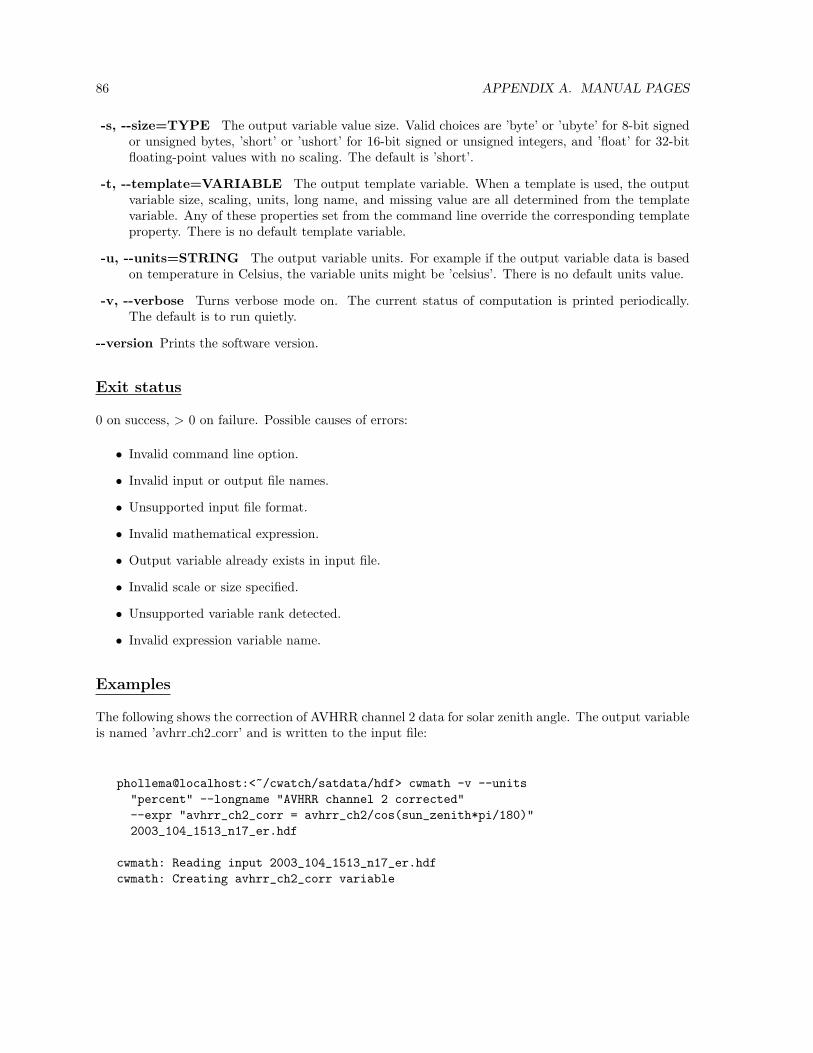
86 APPENDIX A. MANUAL PAGES
-s, --size=TYPE The output variable value size. Valid choices are ’byte’ or ’ubyte’ for 8-bit signedor unsigned bytes, ’short’ or ’ushort’ for 16-bit signed or unsigned integers, and ’float’ for 32-bitfloating-point values with no scaling. The default is ’short’.
-t, --template=VARIABLE The output template variable. When a template is used, the outputvariable size, scaling, units, long name, and missing value are all determined from the templatevariable. Any of these properties set from the command line override the corresponding templateproperty. There is no default template variable.
-u, --units=STRING The output variable units. For example if the output variable data is basedon temperature in Celsius, the variable units might be ’celsius’. There is no default units value.
-v, --verbose Turns verbose mode on. The current status of computation is printed periodically.The default is to run quietly.
--version Prints the software version.
Exit status
0 on success, > 0 on failure. Possible causes of errors:
• Invalid command line option.
• Invalid input or output file names.
• Unsupported input file format.
• Invalid mathematical expression.
• Output variable already exists in input file.
• Invalid scale or size specified.
• Unsupported variable rank detected.
• Invalid expression variable name.
Examples
The following shows the correction of AVHRR channel 2 data for solar zenith angle. The output variableis named ’avhrr ch2 corr’ and is written to the input file:
phollema@localhost:<~/cwatch/satdata/hdf> cwmath -v --units"percent" --longname "AVHRR channel 2 corrected"--expr "avhrr_ch2_corr = avhrr_ch2/cos(sun_zenith*pi/180)"2003_104_1513_n17_er.hdf
cwmath: Reading input 2003_104_1513_n17_er.hdfcwmath: Creating avhrr_ch2_corr variable

A.12. CWMATH 87
cwmath: Computing row 0cwmath: Computing row 100cwmath: Computing row 200cwmath: Computing row 300...
Another example below shows the computation of Normalized Difference Vegetation Index (NDVI):
phollema@localhost:<~/cwatch/satdata/hdf> cwmath -v --longname"Normalized Difference Vegetation Index"--expr "ndvi = (avhrr_ch2 - avhrr_ch1)/(avhrr_ch2 + avhrr_ch1)"2003_104_1513_n17_er.hdf
cwmath: Reading input 2003_104_1513_n17_er.hdfcwmath: Creating ndvi variablecwmath: Computing row 0cwmath: Computing row 100cwmath: Computing row 200cwmath: Computing row 300...
In order to demonstrate the use of the ’mask’ function, the example below shows the masking of the ’sst’variable using the ’cloud’ variable. Note that a hexadecimal value is used to determine which valuesfrom the cloud mask are used in the masking procedure. Since the cloud data is represented by 8-bitbytes, the hexadecimal mask value need only specify two hexadecimal digits. In this case, the value’0x6f’ represents bits 1, 2, 3, 4, 6, and 7 (for all cloud mask bits, the value would be ’0xff’):
phollema@localhost:<~/cwatch/satdata/hdf> cwmath -v --template sst--expr ’sst_masked = mask (sst, cloud, hex ("0x6f"))’2003_104_1513_n17_er.hdf
cwmath: Reading input 2003_104_1513_n17_er.hdfcwmath: Creating sst_masked variablecwmath: Computing row 0cwmath: Computing row 100cwmath: Computing row 200cwmath: Computing row 300...
A final example below shows how the tool may be used to compute complex formulas using a UnixBourne shell script. The example computes the theoretical AVHRR channel 3b albedo at night forNOAA-17 using actual channel 3b temperatures and channel 3b emission temperatures estimated fromchannel 4 and 5:

88 APPENDIX A. MANUAL PAGES
#!/bin/sh
input=$1T3E_A=6.82947T3E_B=0.97232T3E_C=1.66366ZERO_C=273.15t3="(avhrr_ch3 + $ZERO_C)"t4="(avhrr_ch4 + $ZERO_C)"t5="(avhrr_ch5 + $ZERO_C)"t3e="($T3E_A + $T3E_B*$t4 + $T3E_C*($t4 - $t5))"planck_c1=1.1910427e-5planck_c2=1.4387752w3=2669.3554c3b_a=1.702380c3b_b=0.997378rad3="(($planck_c1*($w3^3)) / (e^(($planck_c2*$w3)/($c3b_a + $c3b_b*$t3)) - 1.0))"rad3e="(($planck_c1*($w3^3)) / (e^(($planck_c2*$w3)/($c3b_a + $c3b_b*$t3e)) - 1.0))"alb3="(100*(1 - $rad3/$rad3e))"cwmath -v --longname "AVHRR channel 3 albedo" --units "percent" \--expr "avhrr_ch3_albedo=$alb3" $input

A.13. CWNAVIGATE 89
A.13 cwnavigate
Name
cwnavigate - adds navigation corrections to Earth data.
Synopsis
cwnavigate [OPTIONS] {-t, --trans=ROWS/COLS} inputcwnavigate [OPTIONS] {-r, --rotate=ANGLE} inputcwnavigate [OPTIONS] {-a, --affine=A/B/C/D/E/F} inputcwnavigate [OPTIONS] {-R, --reset} input
Options:
-h, --help-m, --match=PATTERN-v, --verbose--version
Description
The navigation tool adds navigation corrections to 2D variables in an Earth data file by setting naviga-tion transform parameters. The most basic navigation transform consists of additive translation in therow and column data coordinates. As an example of translation, the following diagram shows coastlinesin the Earth image data as a ’.’ (period) symbol and coastlines derived from a GIS database as a ’*’(star). Translation has been used to correct the position of the image data:
*** ***... *** ***** *** *****... *** **... *** **... * .** ----> * **. * ** * **. **** row trans = 1 ****.... col trans = -2
A more generic navigation transform consists of a translation combined with a rotation or shear. Torepresent generic navigation transforms, an affine transform matrix is used to convert “desired” datacoordinates to “actual” data coordinates as follows:

90 APPENDIX A. MANUAL PAGES
|row’| |a c e| |row|| | | | | ||col’| = |b d f| |col|| | | | | || 1 | |0 0 1| | 1 |
where [a..f] are the affine transform matrix coefficients and (row’,col’) is the actual data coordinates atwhich the desired data value for (row,col) may be found.
To apply a navigation transform to a 2D variable, the existing navigation transform is read and the newtransform is applied to it using matrix multiplication to create a combined transform. As an example,suppose that T1 is the initial navigation transform. The application of an additional transform T2results in a new transform that is equivalent to:
T2 (T1 (row, col))
A navigation transform can be applied to a subset of 2D variables, or all variables in the file. Notethat satellite channel data or channel-derived variables should be corrected with navigation but GIS-derived variables such as coastline and lat/lon grid graphics should not be corrected. Setting thenavigation transform simply establishes a mapping between desired and actual data coordinates -- itdoes not change the gridded data values themselves. Once a navigation transform has been set, otherCoastWatch tools in this package will take the transform into account when reading the data.
Parameters
Main parameters:
-t, --trans=ROWS/COLS The translation transform to apply. The actual row and column coordi-nates are calculated by adding the specified row and column translation to the desired coordinates.
-r, --rotate=ANGLE The rotation transform to apply. The actual row and column coordinatesare calculated by rotating the desired row and column coordinates about the data center by thespecified angle in degrees. Positive angles rotate counter-clockwise while negative angles rotateclockwise.
-a, --affine=A/B/C/D/E/F The explicit affine transform to apply. The coefficients are used toform the affine transform matrix (see the Description section above) which is applied to theexisting transform using matrix multiplication.
-R, --reset Specifies that the existing navigation transform should be reset to the identity. Underthe identity transform, no navigation correction is performed.
input The input data file name. The navigation corrections are applied to the input file in-situ.For CoastWatch HDF files, the corrections are applied to individual variables. For CoastWatchIMGMAP files, corrections are applied to the global attributes and the --match option has noeffect. No other file formats are supported.

A.13. CWNAVIGATE 91
Options:
-h, --help Prints a brief help message.
-m, --match=PATTERN The variable name matching pattern. If specified, the pattern is usedas a regular expression to match variable names. Only variables matching the pattern will benavigated. By default, no pattern matching is performed and all variables are navigated.
-v, --verbose Turns verbose mode on. The status of navigation correction is printed periodically.The default is to run quietly.
--version Prints the software version.
Exit status
0 on success, > 0 on failure. Possible causes of errors:
• Invalid command line option.
• Invalid input file name.
• Unsupported input file format.
• Unsupported navigation correction.
Examples
The following example shows the navigation correction of a NOAA-15 CoastWatch HDF data file fromthe Gulf of Mexico:
phollema@localhost:<~/cwatch/satdata> cwnavigate --trans -3/3 -v--match ’(avhrr.*|cloud|sst)’ 2002_328_1326_n15_ml.hdf
cwnavigate: Reading input 2002_328_1326_n15_ml.hdfcwnavigate: Applying navigation correction to avhrr_ch1cwnavigate: Applying navigation correction to avhrr_ch2cwnavigate: Applying navigation correction to avhrr_ch4cwnavigate: Applying navigation correction to cloudcwnavigate: Applying navigation correction to sst
Another example below shows the navigation correction of a NOAA-15 CoastWatch IMGMAP data filefrom the US east coast:
phollema@localhost:<~/cwatch/satdata> cwnavigate --trans -2/1 -v2002_326_1330_n15_er_c2.cwf

92 APPENDIX A. MANUAL PAGES
cwnavigate: Reading input 2002_326_1330_n15_er_c2.cwfcwnavigate: Applying navigation correction

A.14. CWREGISTER 93
A.14 cwregister
Name
cwregister - resamples gridded Earth data to a master projection.
Synopsis
cwregister [OPTIONS] master input output
Options:
-h, --help-m, --match=PATTERN-M, --method=TYPE-O, --overwrite=TYPE-p, --polysize=KILOMETERS-r, --rectsize=WIDTH/HEIGHT-v, --verbose--version
Description
The register tool resamples gridded Earth data to a master projection. A master projection specifiesthe translation between grid row and column coordinates and Earth latitude and longitude coordinates.The master projection file is any valid Earth data file from which a set of row and column dimensionsand Earth transform parameters may be extracted. This includes standard CoastWatch product filesas well as master files created using the cwmaster tool.
Parameters
Main parameters:
master The master projection file name. Note that the master file is not altered in any way. It issimply accessed in order to determine grid and Earth transform parameters.
input The input data file name.
output The output data file name.
Options:
-h, --help Prints a brief help message.

94 APPENDIX A. MANUAL PAGES
-m, --match=PATTERN The variable name matching pattern. If specified, the pattern is used as aregular expression to match variable names. Only variables in the input file matching the patternwill be registered. By default, no pattern matching is performed and all variables are registered.
-M, --method=TYPE The registration resampling method. Valid methods are ’inverse’ and ’mixed’.The inverse resampling method divides the destination into rectangles of bounded physical size (seethe --polysize option), and computes polynomial approximations for the coordinate transformson each rectangle in order to determine a source coordinate for each destination coordinate. Thisis the default method and recommended when the source coordinate transform is smooth andcontinuous in the destination coordinate space such as with AVHRR LAC swath data. The mixedresampling method divides the source into rectangles of certain dimensions (see the --rectsizeoption), computes polynomials on each rectangle similar to the inverse method, and follows with asingle pixel interpolation. This method is recommended when the source coordinate transform isdiscontinuous at regular intervals in the destination coordinate space, such as with MODIS swathdata.
-O, --overwrite=TYPE ADVANCED USERS ONLY. Sets the overwrite policy for ’mixed’ moderesampling: either ’always’ (the default), ’never’, or ’closer’. If during resampling, more than onesource pixel maps to a single destination pixel, this option is used to determine if the new valueshould overwrite the old value. By default, the new value always overwrites the destination pixel(the ’always’ mode). If ’never’ is specified, the first written value is never overwritten. If ’closer’ isspecified, the destination pixel is only overwritten if the source pixel is closer in physical locationto the destination than any previous source pixel.
-p, --polysize=KILOMETERS The polynomial approximation rectangle size in kilometers. Thisoption is only used by the inverse resampling method (see the --method option). The inverseresampling method employs a polynomial approximation to speed up the calculation of datalocations. The polynomial rectangle size determines the maximum allowed size of the resamplingrectangles in the destination. The default polynomial size is 100 km, which introduces an error ofless than 0.15 km for AVHRR LAC data.
-r, --rectsize=WIDTH/HEIGHT The polynomial approximation rectangle size in pixels. Thisoption is only used by the mixed resampling method (see the --method option). The mixedresampling method employs a polynomial approximation to speed up the calculation of data loca-tions. The polynomial rectangle size determines the exact dimensions of the resampling rectanglesin the source. The default polynomial rectangle size is 50/50, which introduces only a small errorfor AVHRR LAC data.
-v, --verbose Turns verbose mode on. The current status of data conversion is printed periodically.The default is to run quietly.
--version Prints the software version.
Exit status
0 on success, > 0 on failure. Possible causes of errors:
• Invalid command line option.
• Invalid master, input or output file names.

A.14. CWREGISTER 95
• Unsupported master or input file format.
Examples
The following shows the registration of NOAA-17 AVHRR channel 2 swath data to a southern Californiamaster:
phollema@localhost:<~/cwatch/satdata/2002_318_1826_n17_mo> cwregister-v --match avhrr_ch2 ws_master.hdf 2002_318_1826_n17_mo.hdf2002_318_1826_n17_ws.hdf
cwregister: Reading master ws_master.hdfcwregister: Reading input 2002_318_1826_n17_mo.hdfcwregister: Creating output 2002_318_1826_n17_ws.hdfcwregister: Adding avhrr_ch2 to resampled gridsGridResampler: Found 1 grid(s) for resamplingGridResampler: Resampling 4788x2048 to 1024x1024GridResampler: Creating location estimatorsGridResampler: Computing row 0GridResampler: Computing row 100GridResampler: Computing row 200GridResampler: Computing row 300GridResampler: Computing row 400GridResampler: Computing row 500GridResampler: Computing row 600GridResampler: Computing row 700GridResampler: Computing row 800GridResampler: Computing row 900GridResampler: Computing row 1000cwregister: Closing files

96 APPENDIX A. MANUAL PAGES
A.15 cwrender
Name
cwrender - performs Earth data visualization.
Synopsis
cwrender {-c, --composite=RED/GREEN/BLUE} [OPTIONS] input outputcwrender {-e, --enhance=VARIABLE1[/VARIABLE2]} [OPTIONS] input output
General options:
-h, --help-v, --verbose--version
Output content and format options:
-a, --noantialias-f, --format=TYPE-i, --indexed-I, --imagecolors=NUMBER-l, --nolegends-m, --magnify=LATITUDE/LONGITUDE/FACTOR-o, --logo=NAME-s, --size=PIXELS | full-T, --tiffcomp=TYPE-W, --worldfile=FILE
Plot overlay options:
-A, --bath=COLOR[/LEVEL1/LEVEL2/...]-b, --bitmask=VARIABLE/MASK/COLOR-C, --coast=COLOR[/FILL]-d, --cloud=COLOR-g, --grid=COLOR-H, --shape=FILE/COLOR[/FILL]-L, --land=COLOR-p, --political=COLOR-S, --nostates-t, --topo=COLOR[/LEVEL1/LEVEL2/...]-u, --group=GROUP

A.15. CWRENDER 97
-w, --water=COLOR-X, --exprmask=EXPRESSION/COLOR
Color enhancement options:
-E, --enhancevector=STYLE/SYMBOL[/SIZE]-F, --function=TYPE-k, --background=COLOR-M, --missing=COLOR-P, --palette=NAME-r, --range=MIN/MAX-U, --units=UNITS
Color composite options:
-B, --bluerange=MIN/MAX-G, --greenrange=MIN/MAX-R, --redrange=MIN/MAX-x, --redfunction=TYPE-y, --greenfunction=TYPE-z, --bluefunction=TYPE
Description
Overview
The render tool performs Earth data visualization by converting 2D data sets in the input file tocolor images. The data values are converted from scientific units to a color using either an enhancementfunction and color palette or by performing a color composite of three data variables -- one for each of thered, green, and blue color components. The resulting Earth data plot may have legends displaying thecolor scale, data origin, date, time, projection info, as well as data overlays showing latitude/longitudegrid lines, coast lines, political boundaries, masks, and shapes.
Overlay colors
Overlay colors may be specified using simple color names such as ’red’, ’gray’, ’cyan’, ’blue’, and ’green’.Overlays may be made to appear slightly transparent (allowing the color behind to show through) byfollowing the color name with a colon ’:’ and a transparency value in percent, for example ’red:50’would make the overlay red with a 50% transparency. Transparency values range from 0 (completelyopaque) to 100 (completely transparent).
Colors may also be specified using explicit hexadecimal notation for red/green/blue color componentsand optional alpha component as follows:
0xAARRGGBB

98 APPENDIX A. MANUAL PAGES
^ ^ ^ ^| | | ----- Blue \| | ------- Green |---- Range: 00 -> ff| --------- Red |----------- Alpha (optional) /
Note that the prepended ’0x’ denotes a hexadecimal constant, and must be used even though it is notpart of the color component values. As an example, the simple color names above may be specified ashexadecimal values:
0xff0000 red0x555555 gray0x00ffff cyan0x0000ff blue0x00ff00 green0x80ff0000 red, 50% transparent
Rendering order
The data view itself (not including the legends) is rendered in such a way that overlays may overlapeach other. For example, latitude/longitude grid lines may fall on top of land polygons because thegrid overlay is rendered after the coastline overlay. Knowing the order in which the data and overlaysare rendered may answer some questions if the data view doesn’t look the way the user expects. Thedata view is rendered in the following order:
1. Before any overlay or data, the data view is filled with a background color (normally white) forvector plots or a missing color (normally black) for color enhancement or color composite plots.
2. Color vectors or image pixels are rendered to the data view. The background or missing color willshow though where no vectors or pixels were rendered.
3. Data overlays are rendered to the view in the following order (see the description of each optionbelow):
• Cloud mask (--cloud )
• Bit masks (--bitmask ), possibly more than one
• Expression masks (--exprmask ), possibly more than one
• Water mask (--water )
• Bathymetric contours (--bath )
• Land mask (--land )
• Coastline and filled land polygons (--coast )
• Political lines (--political )
• Topography contours (--topo )

A.15. CWRENDER 99
• Shape files (--shape ), possibly more than one
• Latitude/longitude grid lines (--grid )
• Overlay groups (--group )
Parameters
Main parameters:
-c, --composite=RED/GREEN/BLUE Specifies color composite mode using the named variables.The data variable values are converted to colors using an individual linear enhancement functionfor each variable. The data values are scaled to the range [0..255] and used as the red, green, andblue components of each pixel’s color. Either this option or --enhance must be specified, but notboth.
-e, --enhance=VARIABLE1[/VARIABLE2] Specifies color enhancement mode using the namedvariable(s). The data variable values are converted to colors using an enhancement function andcolor palette. Either this option or --composite must be specified, but not both. If one variablename is specified, the plot shows color-enhanced image data. If two variable names are specified,the plot shows color-enhanced vectors whose direction is derived using the two variables as vectorcomponents. See the --enhancevector and --background options for settings that are specificto vector plots.
input The input data file name.
output The output image file name. Unless the --format option is used, the file extension indicatesthe desired output format: ’.png’, ’.jpg’, ’.tif’, or ’.pdf’.
General options:
-h, --help Prints a brief help message.
-v, --verbose Turns verbose mode on. The current status of data rendering is printed periodically.The default is to run quietly.
--version Prints the software version.
Output content and format options:
-a, --noantialias Turns off line and font antialiasing. By default, the edges of lines and fonts aresmoothed using shades of the drawing color. It may be necessary to turn off antialiasing if thesmoothing is interfering with the readability of annotation graphics, such as in the case of verysmall fonts. This option only effects raster image output formats such as PNG, GIF and JPEG.
-f, --format=TYPE The output format. The current formats are ’png’ for Portable Network Graph-ics, ’gif’ for Graphics Interchange Format, ’jpg’ for Joint Picture Experts Group, ’tif’ for TaggedImage File Format with geolocation tags (GeoTIFF), ’pdf’ for Portable Document Format, or’auto’ to detect the format from the output file name. The default is ’auto’. The correct choiceof output format is governed by the desired use of the rendered image as follows:

100 APPENDIX A. MANUAL PAGES
• PNG is a non-lossy compressed image format supported by most web browsers and imagemanipulation software. It has similar data compression characteristics to GIF and addition-ally supports 24-bit color images.
• GIF is a non-lossy compressed format also supported by most web browsers and imagemanipulation software. The GIF files produced use LZW compression. Images stored inGIF format are run through a color quantization algorithm to reduce the color map to 256colors or less. Although file sizes are generally smaller than PNG, image quality may becompromised by the reduced color map.
• JPEG is a lossy compressed format that should be used with caution for images with sharpcolor lines such as those found in text and annotation graphics. The JPEG format generallyachieves higher compression than PNG or GIF resulting in smaller image file sizes.
• GeoTIFF is a flexible image format with support for Earth location metadata. Manypopular GIS packages handle GeoTIFF images and allow the user to combine a GeoTIFFbase map image with other sources of raster and vector data. The GeoTIFF images generatedare non-lossy uncompressed image data (unless a compression is specified using --tiffcomp), and can be much larger than the corresponding PNG, GIF, or JPEG. Since GeoTIFFimages are generally destined for import into a GIS system, the use of this format turnson the --nolegends option. In general the GeoTIFFs generated are 24-bit colour images,but when no overlays are specified or the --indexed or --imagecolors options are used, aspecial 8-bit paletted image file is generated and comments describing the data value scalingare inserting into the image description tags.
• PDF is a standard for high quality publishing developed by Adobe Systems and is used foroutput to a printer via such tools as the Adobe Acrobat Reader. In general PDF files areslightly larger than the equivalent PNG but retain highly accurate vector graphics compo-nents such as lines and fonts.
-i, --indexed Short for --imagecolors 256 . See the --imagecolors option below.
-I, --imagecolors=NUMBER The number of colors to use for the index color model of the dataimage, up to 256. Normally the data image uses an unlimited number of colors because thisachieves the best visual rendering quality. But in some cases it may be desirable to make theoutput file smaller by limiting the number of colors to <=256 values and using a index colormodel so that each data pixel can be represented as 8-bit bytes. This option can only be usedwith PNG, GIF, GeoTIFF, and PDF output formats, and only with color enhancements, not colorcomposites. While in index color mode, antialiasing is turned off.
-l, --nolegends Turns the plot legends off. By default, the Earth data view is shown in a frame onthe left and to the right color scale and plot information legends are drawn. With no legends, theEarth data is simply rendered by itself with no frame, borders, or legends.
-m, --magnify=LATITUDE/LONGITUDE/FACTOR The magnification center and factor. Thedata view is set to the specified center and pixel magnification factor. The center position is spec-ified in terms of Earth location latitude and longitude in the range [-90..90] and [-180..180] andthe magnification factor as a fractional number (0..1] where factors > 1 magnify and factors < 1shrink. By default, the data view shows the entire data field with an optimal magnification factorto fit the desired view size (see --size ).
-o, --logo=NAME The logo used for plot legends. The current predefined logo names are ’noaa3d’(the default), ’nasa3d’, ’nws3d’, ’doc3d’, and their corresponding non-3D versions ’noaa’, ’nasa’,

A.15. CWRENDER 101
’nws’, and ’doc’. The predefined logos are named for their respective government agencies: NOAA,NASA, National Weather Service (NWS), and Department of Commerce (DOC). The user mayalso specify a custom logo file name, which can be any PNG, GIF, or JPEG file.
-s, --size=PIXELS | full The Earth data view size in pixels. The data view is normally accompaniedby a set of legends unless the --nolegends option is used. By default, the view size is 512 pixels,plus the size of any legends. If ’full’ is specified rather than a size in pixels, the view size is set tomatch the actual full extent of the data, ie: full resolution.
-T, --tiffcomp=TYPE The TIFF compression algorithm. The valid types are ’none’ for no com-pression (the default), ’deflate’ for ZIP style compression, and ’pack’ for RLE style PackBitscompression. This option is only used with GeoTIFF output.
-W, --worldfile=FILE The name of the world file to write. A world file is an ASCII text file usedfor georeferencing images that contains the following lines:
• Line 1: x-dimension of a pixel in map units
• Line 2: rotation parameter
• Line 3: rotation parameter
• Line 4: NEGATIVE of y-dimension of a pixel in map units
• Line 5: x-coordinate of center of upper left pixel
• Line 6: y-coordinate of center of upper left pixel
World files may be written for any GIF, PNG, or JPEG image. The use of this option turnson the --nolegends option. The convention used in GIS is to name the world file similarly tothe image file, but with a different extension. GDAL expects world files with a “.wld” extension,where as ESRI applications expect “.pgw” for PNG, “.gfw” for GIF, and “.jgw” for JPEG. Usersshould name their world files accordingly.
Plot overlay options:
-A, --bath=COLOR[/LEVEL1/LEVEL2/...] The bathymetric contour color and levels. The coloris specified by name or hexadecimal value (see above). Bathymetric contours are generated forthe specified integer levels in meters. If no levels are specified, contours are drawn at 200 m and2000 m. The default is not to render bathymetric contours.
-b, --bitmask=VARIABLE/MASK/COLOR Specifies that a mask should be rendered on top ofthe data image whose pixels are obtained by a bitwise AND with the mask value. The namedvariable is used to mask the Earth data with the specified color and mask. The color is a nameor hexadecimal value (see above). The mask is a 32-bit integer hexadecimal value specifying themask bits. The bitmask is formed by bitwise ANDing the data value and mask value. If the resultof the operation is non zero, the pixel is colored with the bitmask color. This option is useful foroverlaying graphics on the data image when the graphics are stored as an integer valued variablein the data set. Such variables include cloud and land mask graphics. Multiple values of the--bitmask option may be given, in which case the masks are applied in the order that they arespecified.
-C, --coast=COLOR[/FILL] The coast line color and optional fill color. The colors are specified byname or hexadecimal value (see above). The default is not to render coast lines.

102 APPENDIX A. MANUAL PAGES
-d, --cloud=COLOR The cloud mask color. The color is specified by name or hexadecimal value(see above). Cloud masking requires that a ’cloud’ variable exists in the input file. The default isnot to render a cloud mask.
-g, --grid=COLOR The latitude/longitude grid line color. The color is specified by name or hex-adecimal value (see above). The default is not to render grid lines.
-H, --shape=FILE/COLOR[/FILL] The name and drawing/fill colors for a user-supplied shapefile. The colors are specified by name or hexadecimal value (see above). The only file formatcurrently supported is ESRI shapefile format, and only line and polygon data (no point data).The fill color is optional and is used to fill polygons if any are found in the file. Multiple valuesof the --shape option may be given, in which case the shape overlays are rendered in the orderthat they are specified.
-L, --land=COLOR The land mask color. The color is specified by name or hexadecimal value (seeabove). Land masking requires that a ’graphics’ variable exists in the input file with a land maskat bit 3 where bit numbering starts at 0 for the least significant bit. The default is not to render aland mask. For an alternative to the --land option, try using the --coast option with a fill color.
-p --political=COLOR The political boundaries color. The color is specified by name or hexadecimalvalue (see above). The default is not to render political boundaries.
-S, --nostates Turns off state boundary rendering. The default when --political is specified is to ren-der international and state boundaries. With this option is specified, only international boundariesare rendered.
-t, --topo=COLOR[/LEVEL1/LEVEL2/...] The topographic contour color and levels. The coloris specified by name or hexadecimal value (see above). Topographic contours are generated forthe specified integer levels in meters. If no levels are specified, contours are drawn at 200 m, 500m, 1000 m, 2000 m, and 3000 m. The default is not to render topographic contours.
-u, --group=GROUP The overlay group name to render. Overlay groups are a concept from theCoastWatch Data Analysis Tool (CDAT). CDAT users can save a set of preferred overlays as agroup and then restore those overlays when viewing a new data file. The same group names savedfrom CDAT are available to be rendered here. This is an extremely useful option that allows usersto design a set of overlays graphically and adjust the various overlay properties beyond what canbe achieved using the command line options for cwrender. If specified, this option will cause alloverlays in the group to be drawn on top of any other overlays specified by command line options.
-w, --water=COLOR The water mask color. The color is specified by name or hexadecimal value(see above). Water masking is performed similarly to land masking (see the --land option), butthe sense of the land mask is inverted. The default is not to render a water mask.
-X, --exprmask=EXPRESSION/COLOR Specifies that a mask should be rendered on top of thedata image whose pixels are obtained by evaluating the expression. The color is specified by nameor hexadecimal value (see above). An expression mask is a special type of multipurpose masksimilar to a bitmask (see the --bitmask option above) but which allows the user to specify amathematical expression to determine the mask. If the result of the expression is true (in thecase of a boolean result) or non-zero (in the case of a numerical result), the data image is maskedat the given location with the given color. Multiple values of the --exprmask option may begiven, in which case the masks are applied in the order that they are specified. The syntax for

A.15. CWRENDER 103
the expression is identical to the right-hand-side of a cwmath expression (see the cwmath toolmanual page).
Color enhancement options:
-E, --enhancevector=STYLE/SYMBOL[/SIZE] The color-enhanced vector specifications. Thisoption is only used if two variable names are passed to the --enhance option. The vector stylemay be either ’uvcomp’ or ’magdir’; the default is ’uvcomp’. In uvcomp mode, the variablesthat are passed to the --enhance option are taken to be the U (x-direction) and V (y-direction)components of the vector. In magdir mode, the first variable is taken to be the vector magnitude,and the second to be the vector direction in degrees clockwise from north. The vector symbolmay be either ’arrow’ to draw arrows in the direction of the vector, or ’barb’ to draw WMO windbarbs; the default is ’arrow’. If wind barbs are used, the feathered end of the barb points in thedirection of the wind. Lastly, the size of the vector symbols in pixels may be specified; the defaultsize is 10.
-F, --function=TYPE The color enhancement function. Data values are mapped to the range [0..255]by the enhancement function and range, and then to colors using the color palette. The validenhancement function types are ’linear’, ’stepN’, ’log’, ’linear-reverse’, ’stepN-reverse’, and ’log-reverse’ where N is the number of steps in the function, for example ’step10’. The reverse functionsare equivalent to the non-reversed functions but map data values to the range [255..0] rather then[0..255]. By default, the enhancement function is ’linear’. A log enhancement may be necessarywhen the data value range does not scale well with a linear enhancement such as with chlorophyllconcentration derived from ocean color data.
-k, --background=COLOR The color for the background of vector plots. The color is specified byname or hexadecimal value (see above). The default background color is white.
-M, --missing=COLOR The color for missing or out of range data values. The color is specified byname or hexadecimal value (see above). The default missing color is black.
-P, –palette=NAME The color palette for converting data values to colors. The color palettes aredervied in part from the Interactive Data Language (IDL) v5.4 palettes and have similar names.The valid color palette names are as follows (line indexes are simply for reference):
0 BW-Linear1 HSL2562 RAMSDIS3 Blue-Red4 Blue-White5 Grn-Red-Blu-Wht6 Red-Temperature7 Blue-Green-Red-Yellow8 Std-Gamma-II9 Prism10 Red-Purple11 Green-White-Linear12 Grn-Wht-Exponential

104 APPENDIX A. MANUAL PAGES
13 Green-Pink14 Blue-Red215 16-Level16 Rainbow17 Steps18 Stern-Special19 Haze20 Blue-Pastel-Red21 Pastels22 Hue-Sat-Lightness-123 Hue-Sat-Lightness-224 Hue-Sat-Value-125 Hue-Sat-Value-226 Purple-Red-Stripes27 Beach28 Mac-Style29 Eos-A30 Eos-B31 Hardcandy32 Nature33 Ocean34 Peppermint35 Plasma36 Rainbow237 Blue-Waves38 Volcano39 Waves40 Rainbow1841 Rainbow-white42 Rainbow-black43 NDVI44 GLERL-Archive45 GLERL-30-Degrees46 Chlora-147 Chlora-anom48 Spectrum49 Wind-0-5050 CRW_SST51 CRW_SSTANOMALY52 CRW_HOTSPOT53 CRW_DHW54 StepSeq25
By default, the ’BW-Linear’ palette is used which is a gray scale color ramp from black to white.
-r, --range=MIN/MAX The color enhancement range. Data values are mapped to colors usingthe minimum and maximum values and an enhancement function. By default, the enhancement

A.15. CWRENDER 105
range is derived from the data value mean and standard deviation to form an optimal enhancementwindow of 1.5 standard deviation units around the mean.
-U, --units=UNITS The range and color scale units for the enhancement variable(s). By default,the user must specify the values for the --range option in the standard units indicated in thedata. If the user prefers a different set of units to be used, they may be specified here. Manycommon units are accepted (and various forms of those units), for example ’kelvin’, ’celsius’ and’fahrenheit’ for temperature data, ’knots’, ’meters per second’ or ’m/s’ for windspeed, and ’mgper mˆ-3’ or ’kg/m-3’ for concentration. For other possible unit names, see the conventions usedby the Unidata UDUNITS package and its supported units file.
Color composite options:
-B, --bluerange=MIN/MAX The blue component enhancement range, see --redrange .
-G, --greenrange=MIN/MAX The green component enhancement range, see --redrange .
-R, --redrange=MIN/MAX The red component enhancement range. Data values are mapped tothe range [0..255] using the minimum and maximum values and an enhancement function. Bydefault, the enhancement range is derived from the data value mean and standard deviation toform an optimal enhancement window of 1.5 standard deviation units around the mean.
-x, --redfunction=TYPE The red component enhancement function. Data values are mapped tothe range [0..255] by the enhancement function and range, and then the pixel color is created bycompositing the red, green, and blue mapped values into one 32-bit integer color value. See the--function option for valid function types. By default, the red, green, and blue enhancementsare linear.
-y, --greenfunction=TYPE The green component enhancement function, see --redfunction .
-z, --bluefunction=TYPE The blue component enhancement function, see --redfunction .
Exit status
0 on success, > 0 on failure. Possible causes of errors:
• Invalid command line option.
• Invalid input or output file names.
• Invalid variable name.
• Unrecognized format.
• Unrecognized color name.
• Invalid palette name.
• Invalid magnification center.

106 APPENDIX A. MANUAL PAGES
Examples
As an example of color enhancement, the following command shows the rendering of AVHRR channel2 data from a CoastWatch HDF file to a PNG image, with coast and grid lines in red and the defaultlinear black to white palette. We allow the routine to calculate data statistics on channel 2 for anoptimal enhancement range:
phollema@localhost:<~/cwatch/satdata> cwrender --verbose--enhance avhrr_ch2 --coast red --grid red 2002_288_1435_n17_er.hdf2002_288_1435_n17_er_ch2.png
cwrender: Reading input 2002_288_1435_n17_er.hdfcwrender: Normalizing color enhancementEarthDataView: Preparing data imageEarthDataView: Rendering overlay noaa.coastwatch.render.CoastOverlayEarthDataView: Rendering overlay noaa.coastwatch.render.LatLonOverlaycwrender: Writing output 2002_288_1435_n17_er_ch2.png
For a color composite of the same file, the following command shows the rendering of AVHRR channels1, 2, and 4 to a PNG image. Again, we allow the routine to calculate statistics for optimal enhancementranges. Note that the final enhancement function is reversed in order to map warm AVHRR channel 4values to dark and cold values to bright:
phollema@localhost:<~/cwatch/satdata> cwrender --verbose--composite avhrr_ch1/avhrr_ch2/avhrr_ch4--bluefunction reverse-linear --coast black --grid gray2002_288_1435_n17_er.hdf 2002_288_1435_n17_er_ch124.png
cwrender: Reading input 2002_288_1435_n17_er.hdfcwrender: Normalizing red enhancementcwrender: Normalizing green enhancementcwrender: Normalizing blue enhancementEarthDataView: Preparing data imageEarthDataView: Rendering overlay noaa.coastwatch.render.CoastOverlayEarthDataView: Rendering overlay noaa.coastwatch.render.LatLonOverlaycwrender: Writing output 2002_288_1435_n17_er_ch124.png
A further example below shows the rendering of AVHRR derived sea-surface-temperature data fromthe same file with a cloud mask applied. The color enhancement uses a blue to red color palette andan explicit range from 5 to 20 degrees Celsius:
phollema@localhost:<~/cwatch/satdata> cwrender --verbose--enhance sst --coast white --grid white --palette HSL256

A.15. CWRENDER 107
--range 5/20 --cloud gray 2002_288_1435_n17_er.hdf2002_288_1435_n17_er_sst.png
cwrender: Reading input 2002_288_1435_n17_er.hdfEarthDataView: Preparing data imageEarthDataView: Rendering overlay noaa.coastwatch.render.BitmaskOverlayEarthDataView: Rendering overlay noaa.coastwatch.render.CoastOverlayEarthDataView: Rendering overlay noaa.coastwatch.render.LatLonOverlaycwrender: Writing output 2002_288_1435_n17_er_sst.png
An example usage of the --magnify option is shown below to create a plot of cloud masked sea-surface-temperature data off Nova Scotia:
phollema@localhost:<~/cwatch/satdata> cwrender --verbose--enhance sst --coast white --grid white --palette HSL256--range 5/20 --cloud gray --magnify 43/-66/12002_288_1435_n17_er.hdf 2002_288_1435_n17_er_sst_mag.png
cwrender: Reading input 2002_288_1435_n17_er.hdfEarthDataView: Preparing data imageEarthDataView: Rendering overlay noaa.coastwatch.render.BitmaskOverlayEarthDataView: Rendering overlay noaa.coastwatch.render.CoastOverlayEarthDataView: Rendering overlay noaa.coastwatch.render.LatLonOverlaycwrender: Writing output 2002_288_1435_n17_er_sst_mag.png
Known Bugs
When using the --coast option with a fill color and output is to a PDF file, lakes may contain a thinstripe of land in some places. In this case, use the --land for land filling instead.
When using the --coast option with a fill color, map projection discontinuities or swath projectionedges may not be filled correctly.

108 APPENDIX A. MANUAL PAGES
A.16 cwsample
Name
cwsample - extracts data values at specified Earth locations.
Synopsis
cwsample {-s, --sample=LATITUDE/LONGITUDE} [OPTIONS] input outputcwsample {-S, --samples=FILE} [OPTIONS] input output
Options:
-d, --dec=DECIMALS-D, --delimit=STRING-h, --help-H, --header-i, --imagecoords-m, --match=PATTERN-M, --missing=VALUE-n, --nocoords-R, --reverse-V, --variable=NAME1[/NAME2/...]--version
Description
The sampling tool extracts data values at specified Earth locations from 2D data variables. A samplepoint may be specified on the command line using geographic coordinates, or multiple sample pointsmay be specified using a data file. A number of 2D data variables may be sampled simultaneously. Thesampled values are printed as ASCII text to the output file, one line per sample point. Various optionsare available to modify the output decimals places, delimiters, and so on.
Parameters
Main parameters:
-s, --sample=LATITUDE/LONGITUDE The sample point for a single sampling operation. Thepoint is specified in terms of Earth location latitude and longitude in the range [-90..90] and [-180..180].
-S, --samples=FILE The file name containing a list of sample points for performing multiple sam-pling operations. The file must be an ASCII text file containing sample points as latitude /

A.16. CWSAMPLE 109
longitude pairs, one line per pair, with values separated by spaces or tabs. The points are speci-fied in terms of Earth location latitude and longitude in the range [-90..90] and [-180..180].
input The input data file name.
output The output text file name. If the output file name is ’-’, output is sent to standard output(normally the terminal).
Options:
-d, --dec=DECIMALS The number of decimal places for printed geographic coordinate values.The default is 6 decimals.
-D, --delimit=STRING The value delimiter string. By default, values are separated with a singlespace character.
-h, --help Prints a brief help message.
-H, --header Specifies that a one line header should be written. The header is written before anydata and consists of the output column names. By default no header is written.
-i, --imagecoords Specifies that image coordinates (row and column) should be printed for eachoutput line. The default is to print only geographic coordinates.
-m, --match=PATTERN The variable name matching pattern. If specified, the pattern is usedas a regular expression to match variable names. Only variables matching the pattern will besampled. By default, no pattern matching is performed and all variables are sampled unless the--variable option is used. Note that either --variable or --match may be specified, but notboth.
-M, --missing=VALUE The output value for missing or out of range data. The default is to print’NaN’ for missing values.
-n, --nocoords Turns geographic coordinate printing off. By default, each output line has the form’latitude longitude value(s)’ but with no coordinates, each line simply contains the data value(s).
-R, --reverse Specifies that coordinates should be printed in reverse order, ’longitude latitude’. Thedefault is ’latitude longitude’.
-V, --variable=NAME1[/NAME2/... ] The variable names to sample. If specified, the variablesample values are printed in columns in exactly the same order as they are listed. This optionis different from the --match option because it (i) specifies the column order, where as --matchorders the columns as the variables are encountered in the file, and (ii) does not support patternmatching; all variable names must be specified exactly. Without this option or the --matchoption, all variables are sampled. Note that either --variable or --match may be specified, butnot both.
--version Prints the software version.

110 APPENDIX A. MANUAL PAGES
Exit status
0 on success, > 0 on failure. Possible causes of errors:
• Invalid command line option.
• Invalid input or output file names.
• Invalid sample coordinates file format.
Examples
In the example below, a sample points file named sample locs.txt was set up to follow the 93 W longitudeline at regular 0.2 degree intervals as follows:
28 -9328.2 -9328.4 -9328.6 -9328.8 -9329 -9329.2 -9329.4 -9329.6 -9329.8 -9330 -93
and a Gulf of Mexico data file sampled for SST and cloud data along this line with output to theterminal screen:
phollema@localhost:<~/cwatch/satdata> cwsample --header--match ’(sst|cloud)’ --samples sample_locs.txt2002_325_1546_n17_mr.hdf -
latitude longitude sst cloud28 -93 25.24 028.2 -93 25.24 028.4 -93 24.78 028.6 -93 23.84 028.8 -93 22.72 029 -93 21.37 029.2 -93 20.06 029.4 -93 19.29 029.6 -93 18.16 029.8 -93 17.57 6

A.16. CWSAMPLE 111
30 -93 17.48 22
Another example shows the sampling of one SST value as in the case of comparison with a single buoymeasurement with output to the terminal screen:
phollema@localhost:<~/cwatch/satdata> cwsample --header--match sst --sample 28.8/-93 2002_325_1546_n17_mr.hdf -
latitude longitude sst28.8 -93 22.72
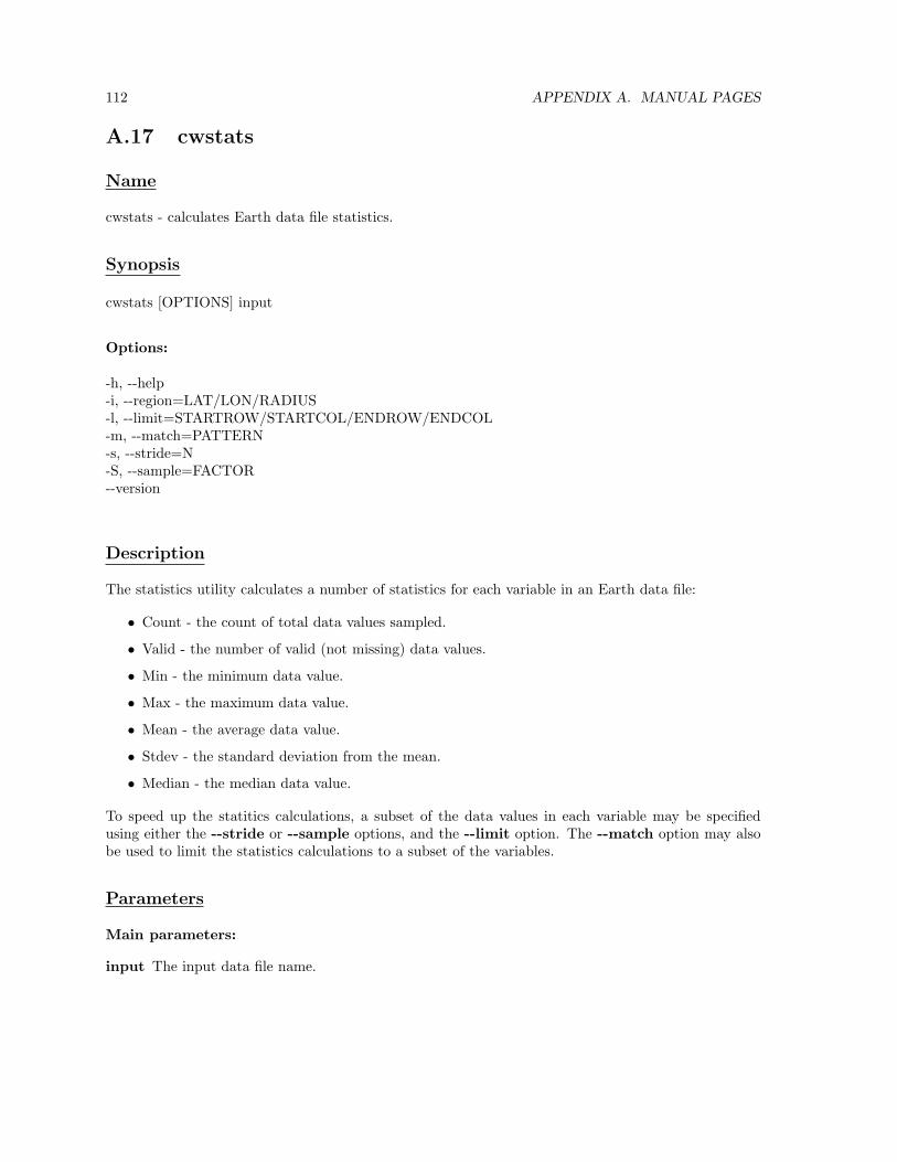
112 APPENDIX A. MANUAL PAGES
A.17 cwstats
Name
cwstats - calculates Earth data file statistics.
Synopsis
cwstats [OPTIONS] input
Options:
-h, --help-i, --region=LAT/LON/RADIUS-l, --limit=STARTROW/STARTCOL/ENDROW/ENDCOL-m, --match=PATTERN-s, --stride=N-S, --sample=FACTOR--version
Description
The statistics utility calculates a number of statistics for each variable in an Earth data file:
• Count - the count of total data values sampled.
• Valid - the number of valid (not missing) data values.
• Min - the minimum data value.
• Max - the maximum data value.
• Mean - the average data value.
• Stdev - the standard deviation from the mean.
• Median - the median data value.
To speed up the statitics calculations, a subset of the data values in each variable may be specifiedusing either the --stride or --sample options, and the --limit option. The --match option may alsobe used to limit the statistics calculations to a subset of the variables.
Parameters
Main parameters:
input The input data file name.

A.17. CWSTATS 113
Options:
-h, --help Prints a brief help message.
-i, --region=LAT/LON/RADIUS The sampling region for each two-dimensional variable. Theregion is specified by the center latitude and longitude in degrees, and the radius from the centerin kilometers. Only data within the rectangle specified by the center and radius is sampled. Bydefault, all data is sampled. Either the --region option or the --limit option may be specified,but not both.
-l, --limit=STARTROW/ENDROW/STARTCOL/ENDCOL The sampling limits for each two-dimensional variable in image coordinates. Only data between the limits is sampled. By default,all data is sampled. Either the --region option or the --limit option may be specified, but notboth.
-m, --match=PATTERN The variable name matching pattern. If specified, the pattern is used asa regular expression to match variable names. Only variables matching the pattern are includedin the calculations. By default, no pattern matching is performed and all variables are included.
-s, --stride=N The sampling frequency for each variable dimension. The default is to sample alldata values (stride = 1).
-S, --sample=FACTOR The sampling factor for each variable. The sampling factor is a value inthe range [0..1] that specifies the number of data values sampled as a fraction of the total numberof data values. To sample 1 percent of all data values, the sample factor would be 0.01. Thedefault is to sample all data values (factor = 1).
--version Prints the software version.
Exit status
0 on success, > 0 on failure. Possible causes of errors:
• Invalid command line option.
• Invalid input file name.
• Unsupported input file format.
• Error reading input data values.
Examples
The following shows a statistics calculation on a CoastWatch HDF file from the Great Lakes:
phollema@localhost:<~/cwatch/satdata> cwstats 2002_197_1719_n16_gr.hdf
Variable Count Valid Min Max Mean Stdev

114 APPENDIX A. MANUAL PAGES
avhrr_ch1 1048576 483728 3.49 74.36 13.059646 11.371605avhrr_ch2 1048576 483728 1.97 71.35 18.520041 9.844144avhrr_ch3a 1048576 483728 0.53 52.84 14.664213 8.88201avhrr_ch4 1048576 483728 -44.8 31.55 11.052207 13.683309avhrr_ch5 1048576 483728 -45.48 27.05 7.978351 13.185983sst 1048576 483728 -44.51 51.43 20.166333 16.714169cloud 1048576 1048576 0 127 23.24175 37.179013sat_zenith 1048576 483728 0.36 0.7 0.466376 0.077153sun_zenith 1048576 483728 0.87 0.95 0.907019 0.022209rel_azimuth 1048576 483728 -0.58 -0.33 -0.465731 0.058149graphics 1048576 1048576 0 14 6.84576 2.931459

A.18. CWSTATUS 115
A.18 cwstatus
Name
cwstatus - shows the status of a CoastWatch data server.
Synopsis
cwstatus [OPTIONS]cwstatus [OPTIONS] host
Options:
-c, --script=PATH-h, --help-s, --splash-o, --operator--version
Description
The status utility shows the status of a CoastWatch data server using a graphical user interface. Theincoming, unprocessed, processing, and online data are shown and continually updated as the serveris processing data. Individual passes with coverage area and preview image may be selected from alist. The status utility is designed for use by research personnel and system operators to monitor aCoastWatch data processing server and select data of interest. Detailed help on the usage of cwstatusis available from within the utility using the menu bar under Help | Help and Support .
Parameters
Main parameters:
host The CoastWatch server host name. There is no default host name. If specified, the host iscontacted and polled for its status immediately after the status utility starts. Otherwise, the usermust connect to the server manually using File | New server on the menu bar.
Options:
-c, --script=PATH ADVANCED USERS ONLY. The query script path. The default is /ctera/query.cgi.
-h, --help Prints a brief help message.
-s, --splash Shows the splash window on startup. The splash window shows the version, author, andweb site information.

116 APPENDIX A. MANUAL PAGES
-o, --operator Specifies that operator messages should be displayed. By default, errors on the serverare not of interest to normal users and are not displayed. Operator messages take the form of aspecial message box that appears when an error occurs.
--version Prints the software version.
Exit status
0 on success, > 0 on failure. Possible causes of errors:
• Invalid command line option.
Examples
The following command shows the startup of the status monitor for the fictitious server foobar.noaa.gov:
phollema@localhost:<~/cwatch/satdata> cwstatus foobar.noaa.gov

A.19. HDATT 117
A.19 hdatt
Name
hdatt - reads or writes HDF file attributes.
Synopsis
hdatt [OPTIONS] inputhdatt {-n, --name=STRING} [OPTIONS] inputhdatt {-n, --name=STRING} {-l, --value=STRING1[/STRING2/...]} [OPTIONS] input
Options:
-h, --help-t, --type=TYPE-V, --variable=STRING--version
Description
The attribute tool reads or writes HDF file attributes using the HDF Scientific Data Sets (SDS) interface.The two modes work as follows:
Read mode In read mode, the tool can read from either the global attribute set (the default), or theattribute set specific to a variable (when then --variable option is specified). It can read eitherall attribute values in the set (the default), or just a single attribute value (when the --nameoption is specified).
Write mode Write mode is specified by the use of the --value option, which provides a value for anamed attribute. In write mode, the user is required to supply an attribute name and value, andoptionally a type. If no type is specified, the type defaults to ’string’ (see the --type option belowfor the meanings of various type names). Attributes may be written to the global attribute set(the default), or to specific variables in the data file using the --variable option.
Note: The attribute tool is currently limited to reading and writing only the signed HDF data types.In read mode, unsigned HDF attribute data are read correctly, but the value displayed as if it weresigned.

118 APPENDIX A. MANUAL PAGES
Parameters
Main parameters:
-n, --name=STRING The name of the attribute to read or write.
-l, --value=STRING1[/STRING2/... ] The value(s) for the named attribute. If specified, thisplaces the tool into write mode, and --name must specify an attribute name. If an attributealready exists, its value is overwritten with the new value. If an attribute with the name does notexist, it is created and the new value assigned to it. By default if this option is not used, the toolis in read mode.
input The input data file name.
Options:
-t, --type=TYPE The attribute data type (write mode only). The valid types and their HDFequivalents are as follows:
Type name HDF typestring DFNT CHAR8byte DFNT INT8short DFNT INT16int DFNT INT32long DFNT INT64float DFNT FLOAT32
double DFNT FLOAT64
-V, --variable=STRING The variable to read or write the attribute data. By default, the attributeis read from or written to the global attribute set.
--version Prints the software version.
Exit status
0 on success, > 0 on failure. Possible causes of errors:
• Invalid command line option.
• Invalid input or output file names.
• Invalid variable name.
• Invalid attribute name in read mode.
• Invalid attribute type in write mode.
• Value does not convert to the specified attribute data type.

A.19. HDATT 119
Examples
As an example of read mode, the following command reads and prints all the global attribute data froma CoastWatch HDF file:
phollema@damdog<~/cwatch/satdata/level3> hdatt 2005_095_1522_n17_er.hdfsatellite = noaa-17sensor = avhrrorigin = USDOC/NOAA/NESDIS CoastWatchcwhdf_version = 3.2pass_type = daypass_date = 12878start_time = 55371.0projection_type = mappedprojection = Mercatorgctp_sys = 5gctp_zone = 0gctp_parm = 0.0 0.0 0.0 0.0 0.0 0.0 0.0 0.0 0.0 0.0 0.0 0.0 0.0 0.0 0.0gctp_datum = 12et_affine = 0.0 -1470.0 1470.0 0.0 -8804259.100925786 5723777.271647277rows = 1401cols = 1302polygon_latitude = 45.83810150571052 45.83810150571052 45.8381015057105245.83810150571052 45.83810150571052 42.51315402540104 38.9999999999871935.30179546333813 31.424886223357582 31.424886223357582 31.42488622335758231.424886223357582 31.424886223357582 35.30179546333813 38.9999999999871942.51315402540104 45.83810150571052
polygon_longitude = -79.09000515710031 -74.79500257855015 -70.5 -66.20499742144985-61.90999484289969 -61.90999484289969 -61.90999484289969 -61.90999484289969-61.90999484289969 -66.20499742144985 -70.5 -74.79500257855015 -79.09000515710031-79.09000515710031 -79.09000515710031 -79.09000515710031 -79.09000515710031
history = cwimport product.tshdf product.hdf
To dump only a single attribute:
phollema@damdog<~/cwatch/satdata/level3> hdatt --name satellite2005_095_1522_n17_er.hdf
noaa-17
or a single attribute from a specific variable:
phollema@damdog<~/cwatch/satdata/level3> hdatt --name units--variable avhrr_ch3a 2005_095_1522_n17_er.hdf

120 APPENDIX A. MANUAL PAGES
albedo*100%
As an example of write mode, suppose that we wanted to save the date when the file was originallydownloaded from the server:
phollema@damdog<~/cwatch/satdata/level3> hdatt --name download_date--value "Mon Apr 11 18:20:15 PDT 2005" 2005_095_1522_n17_er.hdf
Now suppose we wanted to assign an integer quality value of 65% to the file based on some test thatwas performed on the file data:
phollema@damdog<~/cwatch/satdata/level3> hdatt --name quality_value--value 65 --type int 2005_095_1522_n17_er.hdf
Finally, suppose that we wanted to change the units and scaling factor / offset of a variable, originallyin degrees Celsius and scaled by 0.01, to degrees Fahrenheit:
phollema@damdog<~/cwatch/satdata/level3> hdatt --name units--value "deg F" --variable sst 2005_095_1522_n17_er.hdf
phollema@damdog<~/cwatch/satdata/level3> hdatt --name scale_factor--value 0.018 --type double --variable sst 2005_095_1522_n17_er.hdf
phollema@damdog<~/cwatch/satdata/level3> hdatt --name add_offset--value -1777.777777 --type double --variable sst2005_095_1522_n17_er.hdf

Appendix B
CoastWatch HDF MetadataSpecification
B.1 Overview
CoastWatch HDF format may be used to store almost any scientific data that has an associated setof Earth locations, including satellite data and output from numerical models. The term metadatarefers to information describing data. HDF stores metadata as a set of attribute name and value pairs.For example, if a dataset is derived from a satellite called NOAA-16, it is useful to store the attributename satellite and value noaa-16 along with the data to denote its origin. Along these lines, theCoastWatch metadata standards have been written to help developers write software to read and writedata and its associated metadata in a consistent fashion. This document describes the standard andcan be used as a reference guide to the HDF attribute names and values in CoastWatch HDF files. Anumber of overall conventions are used for storing data:
1. Multiple 2D data grids are stored in one HDF file using the HDF Scientific Data Sets (SDS)model. A standard CoastWatch HDF file contains data for one region only.
2. A standard set of global attributes is encoded with the data, describing the date and time, Earthlocations, data source or satellite/ sensor, and so on from which the data originated.
3. A standard set of variable attributes is encoded with each variable, describing the variable units,scaling factor, and so on as well as any other important information.
As the requirements for the CoastWatch HDF format evolve, new metadata specifications are added,thus new metadata versions support features that older versions do not. An effort is made with eachnew metadata version to maintain compatibility with older versions:
Version 2.4 The original metadata version supported by the CWF utilities version 2.3 and 2.4 andCDAT 0.6 and 0.7. CoastWatch HDF was originally designed to store projection-mapped satellitedata only, and had a very limited set of metadata.
121

122 APPENDIX B. COASTWATCH HDF METADATA SPECIFICATION
Version 3.1 Support was added for multiple metadata versions, unmapped swath data, per-variablenavigation transforms, and the interpretation of the et affine attribute was changed.
Version 3.2 Support was added for non-satellite derived data, composite datasets from multiple timeranges, raster pixel types, region codes and names, temporal extents, vector direction variables,polygon outlines, and various other features.
Version 3.3 Support was added for satellite sensor scan projection type.
Version 3.4 Units strings were standardized to use Unidata UDUNITS style. Vector direction variablesnow have a convention attribute.
B.2 Global Metadata
The following table lists the standard set of global attributes for CoastWatch HDF:
Attribute name HDF type Description Since versioncwhdf version† CHAR8 The metadata version. The version is written as
a string attribute but should be interpreted asa fractional number, for example 2.3 or 3.1. Ifabsent, version 2.4 is assumed.
3.1
satellite‡ CHAR8 If data is from a satellite, the satellite name, forexample noaa-16, goes-8, orbview-2.
2.4
CHAR8 If the data is a composite, multiple values arenewline-separated.
3.2
sensor‡ CHAR8 If data is from a satellite, the satellite sensorname, for example avhrr, seawifs.
2.4
CHAR8 If the data is a composite, multiple values arenewline-separated.
3.2
data source‡ CHAR8 If data is not from a satellite, the data source, forexample the instrument used to collect the dataor the model used to generate the data. If thedata is a composite, multiple values are newline-separated.
3.2
composite CHAR8 The composite flag, true if the data is de-rived from multiple datasets, or false if not.If true, then the pass date, start time, andtemporal extent attributes may contain ar-rays of values, and the satellite, sensor,data source, orbit type, pass type, andorigin attributes may have multiple newline-separated values. If absent, it is assumed thatthe data is not a composite.
3.2

B.3. EARTH LOCATION METADATA 123
Attribute name HDF type Description Since versionpass date† INT32 The date of data recording in days since January
1, 1970.2.4
INT32[ ] If the data is a composite, the dates of datarecording in days since January 1, 1970. Dateand time data must be stored in sorted order fromleast recent to most recent.
3.2
start time† FLOAT64 The start time of the data recording in secondssince 00:00:00 UTC.
2.4
FLOAT64[ ] If the data is a composite, the start times of datarecording in seconds since 00:00:00 UTC.
3.2
temporal extent FLOAT64[ ] The time duration in seconds between the startof data recording and the end of data recording.Multiple values may be present if the data is acomposite. If absent, it is assumed that each datarecording is instantaneous.
3.2
pass type CHAR8 The satellite pass temporal type: day, night,day/night.
2.4
CHAR8 If the data is a composite, multiple values arenewline-separated.
3.2
orbit type CHAR8 If the data is from an orbiting satellite thatcrosses the equator in a northward or south-ward direction, the orbit type as ascending ordescending respectively. If the data is a com-posite, multiple values are newline-separated.
3.2
origin† CHAR8 The original data source as an agency or orga-nization name, for example USDOC/NOAA/NESDISCoastWatch.
2.4
CHAR8 If the data is a composite, multiple values arenewline-separated.
3.2
history† CHAR8 A newline-separated list of utilities and commandline parameters used to create the file and per-form processing.
2.4
†This attribute is required. Other attributes are optional.‡Either satellite and sensor, or data source are required, but not both.
B.3 Earth Location Metadata
In addition to the standard global attributes listed above, a number of Earth location attributes are alsopresent. Prior to version 3.1, only mapped data was supported. For mapped data, all map projectioncalculations are performed using the General Cartographic Transformation Package (GCTP) from theUSGS National Mapping Division. A number of global attributes are dedicated to storing GCTP relatedparameters. For documentation on the allowed values of GCTP parameters, see section B.6. The tablebelow lists the standard set of global attributes for Earth location metadata:

124 APPENDIX B. COASTWATCH HDF METADATA SPECIFICATION
Attribute name HDF type Description Since versionprojection type † CHAR8 The projection type: mapped, swath, or
sensor scan. Mapped data is formatted to awell-known map projection and accompanied byGCTP map projection parameters. Swath datais data that is not in a standard map projection,but is accompanied by Earth location data foreach pixel (see section B.5 on swath data). Sensorscan data is similar to swath in that it cannot bedescribed by a set of map projection parameters,but it can be described by a set of sensor-specificparameters and does not require Earth locationsto be stored for each pixel.
3.1
projection‡ CHAR8 For mapped data, a descriptive projectionname, for example mercator, geographic, polarstereographic.
2.4
gctp sys‡ INT32 For mapped data, the GCTP projection systemcode.
2.4
gctp zone‡ INT32 For mapped data, the GCTP zone for UTM pro-jections.
2.4
gctp parm‡ FLOAT64[ ] For mapped data, the GCTP projection parame-ters (15).
2.4
gctp datum‡ INT32 For mapped data, the GCTP spheroid code. 2.4et affine‡ FLOAT64[ ] For mapped data, the map affine transform (6). 2.4sensor code∗ INT32 For sensor scan data, the sensor code. The only
code currently available is 0, which indicates ageostationary satellite.
3.3
sensor parm∗ FLOAT64[ ] For sensor scan data, the sensor parameters. Fora geostationary satellite (sensor code=0):
1. Subpoint latitude in degrees (geocentric).
2. Subpoint longitude in degrees.
3. Distance of satellite from center of Earth inkilometers.
4. Scan step angle in row direction in radians.
5. Scan step angle in column direction in radi-ans.
3.3
rows† INT32 The number of rows of data. 2.4cols† INT32 The number of columns of data. 2.4polygon latitude FLOAT64[ ] Latitude components of the bounding polygon
with initial element repeated.3.2
polygon longitude FLOAT64[ ] Longitude components of the bounding polygonwith initial element repeated.
3.2

B.3. EARTH LOCATION METADATA 125
Attribute name HDF type Description Since versionraster type CHAR8 One of RasterPixelIsArea or
RasterPixelIsPoint to capture the samedistinction as the GeoTIFF global attributeGTRasterTypeGeoKey. If pixels represent pointdata, then extra SDS variables latitude andlongitude in the dataset localize the pointwithin the pixel area which otherwise defaults tothe pixel center. If absent, pixels are assumed torepresent area data.
3.2
region code CHAR8 The data processing region code as a short abbre-viation.
3.2
region name CHAR8 The data processing region name in full. 3.2station code CHAR8 The data capture ground station as a short ab-
breviation.3.2
station name CHAR8 The data capture ground station name in full. 3.2†This attribute is required. Other attributes are optional.‡Required for mapped data only.∗Required for sensor scan data only.
B.3.1 Version 2 Affine
The et affine attribute is used by CoastWatch software to translate between map (x,y) coordinatesin meters and image (row,col) coordinates. GCTP is used to translate between (lat,lon) in degrees andmap (x,y) in meters. With this two-step process, the translation between image (row,col) and Earthlocation (lat,lon) is very flexible and can be expressed partly as a linear coordinate transform. Thesix affine transform parameters are used in a matrix equation as follows. Let a..f be the et affineattribute array values 0..5, (X, Y ) be map coordinate easting and northing in meters, and (R,C) be1-relative row and column image coordinates, then: X
Y1
=
a b ec d f0 0 1
CR1
or alternatively:
X = aC + bR + e
Y = cC + dR + f
The inverse operation may be performed by inverting the affine transform:
α = ad− bc
a′ = d/α
b′ = −b/α
c′ = −c/α
d′ = a/α
e′ = −(a′e + b′f)f ′ = −(c′e + d′f)

126 APPENDIX B. COASTWATCH HDF METADATA SPECIFICATION CR1
=
a′ b′ e′
c′ d′ f ′
0 0 1
XY1
or alternatively:
C = a′X + b′Y + e′
R = c′X + d′Y + f ′
B.3.2 Version 3 Affine
The conventions of the et affine attribute are slightly different in version 3 metadata. The affinetransform is stored and used (in matrix form) as:
XY1
=
a c eb d f0 0 1
RC1
or alternatively:
X = aR + cC + e
Y = bR + dC + f
where (R,C) are 0-relative, not 1-relative image coordinates. Deriving the inverse transform is similarlychanged.
B.4 Variable Metadata
The following table shows the standard set of variable attributes for CoastWatch HDF. Some attributegroups are created by HDF SD convenience functions in order to make data more readable and usableby generic HDF viewing programs. A <var> in the HDF Type indicates that the attribute type is thesame as the variable data type.

B.4. VARIABLE METADATA 127
Attribute name HDF type Description Since versionlong name† CHAR8 Written by SDsetdatastrs. A descriptive vari-
able name, for example AVHRR channel 4, seasurface temperature.
2.4
units† CHAR8 Written by SDsetdatastrs. A descriptive unitsname in the conventions used by the UnidataUDUNITS package and its supported units file.Many common units are acceptable (and vari-ous forms of those units), for example kelvin,celsius and fahrenheit for temperature data,knots, meters per second or m/s for wind-speed, mg per m^-3 or kg/m-3 for concentration,percent or % for reflectance, and degrees orradians for angles.
2.4, updated in 3.4
format† CHAR8 Written by SDsetdatastrs. A FORTRAN-77 styleformat string, for example F7.2.
2.4
coordsys† CHAR8 Written by SDsetdatastrs. A descriptive coor-dinate system name, the same as the globalprojection attribute.
2.4
FillValue <var> Written by SDsetfillvalue. The value used to fillin for missing or unwritten data.
2.4
scale factor‡ FLOAT64 Written by SDsetcal. The calibration scale factor. 2.4scale factor err‡ FLOAT64 Written by SDsetcal. The calibration scale error. 2.4add offset‡ FLOAT64 Written by SDsetcal. The calibration offset. 2.4add offset err‡ FLOAT64 Written by SDsetcal. The calibration offset error. 2.4calibrated nt‡ INT32 Written by SDsetcal. The HDF data type code
for uncalibrated data.2.4
C format† CHAR8 A C style format string, for example %7.2f. 2.4missing value <var> The value used to fill in for missing or unwritten
data; same as FillValue.2.4
fraction digits† INT32 The number of significant digits after the deci-mal place for calibrated or floating-point variabledata. This is an alternative to the C or FOR-TRAN notation for value formatting and is inde-pendent of the programming language.
3.1
nav affine FLOAT64[ ] The navigation correction affine transform. If ab-sent, an identity transform is assumed.
3.1
direction variable CHAR8 The name of the associated SDS variable for vec-tor direction. Any variable with this attributeis assumed to be the magnitude component of avector field, for which the named variable is thedirection component. The direction componentis encoded as degrees clockwise from north.
3.2

128 APPENDIX B. COASTWATCH HDF METADATA SPECIFICATION
Attribute name HDF type Description Since versiondirection convention CHAR8 When this SDS variable is the direction compo-
nent of a vector, the convention for the directionis either DirectionIsTo or DirectionIsFrom toindicate that the direction indicates where to vec-tors are pointing to, or pointing from. For exam-ple, wind direction is normally quoted as wherethe wind is coming from, where as ocean cur-rents are quoted as where the current is mov-ing towards. This attribute is only requiredfor direction component SDS variables (see thedirection variable attribute).
3.4
quality flag CHAR8 The name of the associated SDS variable thatcontains quality flag information.
3.2
quality mask INT64 The value to use as a mask in a bitwise ANDoperation to isolate the quality bits in the SDSvariable named by the quality flag attribute.
3.2
flag bits CHAR8 The newline-separated list of flag descriptions foreach bit from least significant to most significant.This is generally only required if this SDS variablecontains quality flag information for another SDSvariable. Any unused bits are denoted by Unused.
3.2
† This attribute is required. Other attributes are optional.‡ Required for calibrated data only.
B.4.1 Calibration Values
The calibration attributes are used to read and write variable data as follows:
float = scale factor(int− add offset) (on read)int = float/scale factor + add offset (on write)
where float and int are the floating-point and integer values respectively. See the HDF User’s Guidefor more details on data calibration. If no calibration data is found, the data is assumed to be alreadycalibrated.
B.4.2 Navigation Correction
The navigation correction transform has 6 coefficients, similar to the global et affine attribute, andis used (in matrix form) as: R′
C ′
1
=
a c eb d f0 0 1
RC1
wherea..f are the nav affine matrix coefficients in order and (R′, C ′) are the actual image coordinatesat which the desired data value for (R,C) may be found.

B.5. SWATH EARTH LOCATION ENCODING 129
B.5 Swath Earth Location Encoding
There are currently two methods for specifying Earth location data for CoastWatch HDF swath files:
1. Explicit encoding: Two standard 2D HDF SDS variables named latitude and longitude arewritten to the file. Each variable must be accompanied with appropriate metadata as outlinedabove. The latitude and longitude data must not have any values set to the missing or fill value,or problems may occur in performing Earth coordinate transformations.
2. Polynomial encoding: A number of 1D HDF SDS variables named swath struct, swath bounds,swath lat, and swath lon are used to define data structures for use in a polynomial approximationalgorithm that supports an efficient and accurate estimation of latitude and longitude values forthe swath data.
The polynomial encoding option is described in this section. The polynomial approximation scheme isgiven, along with details on the required HDF variables.
The easiest approach to swath Earth location encoding is to simply record latitude and longitude valuesfor every data value in the swath. For a typical AVHRR swath size of 2048×5000, this can add about 80Mb of extra data to a file using 32-bit floating point values. To convert a data (row,col) coordinate togeographic (lat,lon) coordinate, an application simply reads the (lat,lon) data at the specified coordinatefrom the file. This method requires either a large amount of file I/O or a large amount of memory,depending on how much of the Earth location data is read at once. It also does not lend itself to anefficient reverse lookup algorithm for converting an arbitrary (lat,lon) back to (row,col).
In order to support swath data in CoastWatch HDF files but avoid the overhead of storing the Earthlocations, a polynomial approximation scheme is used. The approximation scheme also lends itself toan efficient reverse lookup algorithm. The approximation divides the data into a number of rectangularpartitions of varying size in rows and columns but bounded physical size in kilometres. For a typicalAVHRR swath whose resolution is lowest at the left and right edge of the image data, the rectangularpartitioning may look something like Figure B.1.
The approximation derives a set of bivariate polynomials on each partition for latitude and longitudeestimation. To convert a (row,col) coordinate to (lat,lon), the partitions are first searched for the onecontaining the data coordinate. Using the polynomials for that partition, latitude and longitude arecalculated for the data coordinate using the polynomial coefficients. By bounding the physical size ofeach partition, it is possible to bound the error in latitude and longitude estimation. For a typicalAVHRR pass, it has been found that a 100 km maximum partition size yields a maximum error ofapproximately 50 m in Earth location.
The polynomial approximation scheme used is as follows. For each partition, nine latitude and longitudevalues are sampled in a 3×3 grid pattern as shown in Figure B.2. The (row,col) coordinates and (lat,lon)data values are used to derive two independent sets of 9 polynomial coefficients, one set for latitude andone set for longitude. These coefficients, denoted a0..a8 and b0..b8 can be used to recover the latitudeand longitude values using the formulae:
lat(x, y) = a0 + a1x + a2x2 + a3y + a4xy + a5x
2y + a6y2 + a7xy2 + a8x2y2
lon(x, y) = b0 + b1x + b2x2 + b3y + b4xy + b5x
2y + b6y2 + b7xy2 + b8x
2y2

130 APPENDIX B. COASTWATCH HDF METADATA SPECIFICATION
samples
lines
Figure B.1: A partitioning of AVHRR swath data. Each partition has a bounded physical size in thelines and samples directions.

B.5. SWATH EARTH LOCATION ENCODING 131
Figure B.2: Sampling pattern for polynomial approximation. Each • symbol is a sampling point forlatitude and longitude.
where x is the image row and y is the image column. Note that the polynomial approximation also actsto interpolate (lat,lon) coordinates between integer data coordinates, since there are no requirements onx and y to be integers in the above equations. This is important for the accuracy of the reverse-lookupalgorithm described later.
Since each partition is associated with its own set of coefficients, a simple algorithm to search forthe appropriate partition for a data (row,col) coordinate is to loop through all partitions, checkingthe row and column bounds on each partition until one containing the desired (row,col) coordinate isfound. If there are n partitions, then the loop will perform O(n) (where O() denotes an order of upperbound relationship) partition bound checks. In order to avoid this, a binary tree is used to arrangethe partitions in a hierarchical structure. The set of partitions with polynomial coefficients form theleaves of the tree. The relationship between parent and child nodes is such that each child is a binarysub-partition of the parent. In this way, a search through n partitions is replaced by a search down thebinary tree through O(log n) partitions until a leaf is encountered. For encoding purposes, a binary treestructure may be encoded uniquely using a preorder traversal of its nodes. A 0 is used to encode a leftchild, and a 1 for a right child (the root is not recorded because we assume that the preorder traversalstarts at the root). Figure B.3 shows the binary tree for the encoding 000111. A more complex examplein Figure B.4 show the binary tree for the encoding 000111001101.
For a complete encoding of the swath including the polynomial coefficients for each leaf partition, allpartition boundaries, and the binary tree structure, the following HDF variables are used:

132 APPENDIX B. COASTWATCH HDF METADATA SPECIFICATION
Figure B.3: Binary tree encoding example. The tree is encoded under a preorder traversal by thebinary string 000111.
Figure B.4: A more complex binary tree encoding example. The tree is encoded under a preordertraversal by the binary string 000111001101.

B.5. SWATH EARTH LOCATION ENCODING 133
Variable name HDF type Descriptionswath struct INT8 A preorder encoding of the binary tree. The en-
coding bits are zero-padded at the end to thenearest byte.
swath bounds FLOAT64 Upper-left and lower-right (row,col) bounds foreach partition. All partition bounds are recorded,including all leaf and non-leaf partitions in thetree.
swath lat FLOAT64 Latitude polynomial coefficients for each leaf par-tition. There are 9 coefficients stored for eachpartition.
swath lon FLOAT64 Longitude polynomial coefficients for each leafpartition. There are 9 coefficients stored for eachpartition.
This encoding may be used to re-create the tree structure and populate the tree with partition boundand polynomial information. For a typical AVHRR pass which might require 80 Mb of data if all(lat,lon) coordinates were pre-computed, this encoding only requires about 500 kb using a maximumpartition size of 100 km.
Finally, the reverse-lookup algorithm to convert (lat,lon) coordinates back to (row,col) is as follows.Define the following symbols:
Let T be a tolerance distance in kilometers.Let −→C
in
g be the input geographic (lat,lon) coordinate.
Let −→Cout
d be the output data (row,col) coordinate.Let D−→
C g
(−→C d) be a function that computes the physical distance in kilometers between
geographic coordinate −→C g and data coordinate −→C d.Let Nr and Nc be the total number of rows and columns.Let −→∇d be the gradient operator in data coordinates, −→∇d = ( ∂
∂r , ∂∂c ).
Now, initialize −→Cout
d and iterate until the tolerance is satisfied:
−→C
out
d = (Nr/2, Nc/2)d = D−→
Cin
g
(−→Cout
d )
while d > T {−→u = −→∇dD−→C g
(−→C d)
u = −→u /|−→u |−→C
out
d = −→C
out
d − du
d = D−→C
in
g
(−→Cout
d )
}
This algorithm is particularly well suited to be used with a polynomial approximation scheme for(lat,lon) because it can provide sub-pixel accuracy in the (row,col) coordinate. For example as part of

134 APPENDIX B. COASTWATCH HDF METADATA SPECIFICATION
a data resampling algorithm, once a fractional data coordinate is obtained for a given (lat,lon), nearestneighbour or bilinear interpolation may then be used to provide a smooth data resampling.
B.6 GCTP Appendices
Function Description********************
gctp - Initializes projection transformation parameters and performstransformations.
SYNTAX
FUNCTION gctp (incoor, insys, inzone, inparm, inunit, indatum, ipr,efile, jpr, pfile, outcoor, outsys, outzone, outparm, outunit,outdatum, fn27, fn83, iflg)
double incoor[2];long *insys;long *inzone;double inparm[15];long *inunit;long *indatum;long *ipr;char efile[];long *jpr;char pfile[];double outcoor[2];long *outsys;long *outzone;double outparm[15];long *outunit;long *outdatum;char fn27[];char fn83[];long *iflg;
PARAMETERS
* incoor (input, double, length(2))
Array of two input coordinates (X-Y, Longitude-Latitude,Northing-Easting, etc) to be translated. The nature of thecoordinates is defined by insys, inzone, and inunit. The east-westdimension (X, Longitude, Easting) is first followed by thenorth-south (Y, latitude, Northing).

B.6. GCTP APPENDICES 135
* insys (input, long)
Defines the input projection system. Valid codes are:= 0: GEO (Geographic)= 1: UTM (Universal Transverse Mercator)= 2: SPCS (State Plane Coordinates)= 3: ALBERS (Albers Conical Equal Area)= 4: LAMCC (Lambert Conformal Conic)= 5: MERCAT (Mercator)= 6: PS (Polar Stereographic)= 7: POLYC (Polyconic)= 8: EQUIDC (Equidistant Conic)= 9: TM (Transverse Mercator)= 10: STEREO (Stereographic)= 11: LAMAZ (Lambert Azimuthal Equal Area)= 12: AZMEQD (Azimuthal Equidistant)= 13: GNOMON (Gnomonic)= 14: ORTHO (Orthographic)= 15: GVNSP (General Vertical Near-Side Perspective)= 16: SNSOID (Sinusoidal)= 17: EQRECT (Equirectangular)= 18: MILLER (Miller Cylindrical)= 19: VGRINT (Van der Grinten)= 20: HOM (Hotine Oblique Mercator--HOM)= 21: ROBIN (Robinson)= 22: SOM (Space Oblique Mercator--SOM)= 23: ALASKA (Modified Stereographic Conformal--Alaska)= 24: GOOD (Interrupted Goode Homolosine)= 25: MOLL (Mollweide)= 26: IMOLL (Interrupted Mollweide)= 27: HAMMER (Hammer)= 28: WAGIV (Wagner IV)= 29: WAGVII (Wagner VII)= 30: OBLEQA (Oblated Equal Area)
* inzone (input, long)
Input zone for UTM and State Plane projection systems. The UTMCoordinate System (insys = 1) and State Plane Coordinate System(insys = 2) use zone codes instead of specific projection parameters(See Appendix B--UTM and Appendix C--State Plane). For SouthernHemisphere UTM, use a negative zone code. Inzone will be ignored forall other projections.
* inparm (input, double, length(15))
Array of fifteen projection parameters. These parameters are

136 APPENDIX B. COASTWATCH HDF METADATA SPECIFICATION
required to define each map projection. (See Appendix A)
* inunit (input, long)
Unit code for input coordinates. Valid unit codes are:= 0: radians= 1: U.S. feet= 2: meters= 3: seconds of arc= 4: degrees of arc= 5: International feet= 6: Table supplying the unit code, which is legislated
for the State zone selected
* indatum (input, long)
Input spheroid code. This identifies the semi-major axis andeccentricity that is to be used in the transformation process. If anegative spheroid code is entered, inparm elements 1 and 2 are to beused (See Appendix A). Supported spheroids include:= 0: Clarke 1866 (default)= 1: Clarke 1880= 2: Bessel= 3: International 1967= 4: International 1909= 5: WGS 72= 6: Everest= 7: WGS 66= 8: GRS 1980= 9: Airy= 10: Modified Everest= 11: Modified Airy= 12: WGS 84= 13: Southeast Asia= 14: Australian National= 15: Krassovsky= 16: Hough= 17: Mercury 1960= 18: Modified Mercury 1968= 19: Sphere of Radius 6370997 meters
Note: State Plane projection (insys = 2) only supports Clarke 1866(indatum = 0) and GRS 1980 (indatum = 8) spheroids corresponding todatums NAD27 and NAD83 respectively (See Appendix B).
* ipr (input, long)
Error message print flag. If ipr is zero, error messages will be
B.6. GCTP APPENDICES 137
printed to the terminal. If ipr is one, error messages will beprinted to efile. If ipr is two, error messages will be printed toboth the terminal and efile. If ipr is something else, errormessages will not be printed.
* efile (input, character, length(*))
The file which will contain the output error messages. efile neednot be opened at this time.
* jpr (input, long)
Projection parameter print flag. If jpr is zero, projectionparameters will be printed to the terminal. If jpr is one,projection parameters will be printed to pfile. If jpr is two,projection parameters will be printed to both the terminal andpfile. If jpr is something else, the projection parameters will notbe printed. As specified by jpr, Projection parameters are printedeach time the input projection parameters (insys, inzone, inparm,inunit, indatum, outsys, outzone, outparm, outunit, and outdatum)change.
* pfile (input, character, length(*))
The file which will contain the output projection parametermessages. pfile need not be opened at this time.
* outcoor (output, double, length(2))
Array of two transformed coordinates. See incoor for an explanation.
* outsys (input, long)
Defines the output projection system. See insys.
* outzone (input, long)
Output zone for UTM and State Plane projection systems. The UTMCoordinate System (outsys = 1) and State Plane Coordinate System(outsys = 2) use zone codes instead of specific projectionparameters (See Appendix B--UTM and Appendix C--State Plane). ForSouthern Hemisphere UTM, use a negative zone code. Outzone will beignored for all other projections.
* outparm (input, double, length(15))
Array of fifteen projection parameters. These parameters arerequired to define each map projection. (See Appendix A)

138 APPENDIX B. COASTWATCH HDF METADATA SPECIFICATION
* outunit (input, long)
Unit code for output coordinates. See inunit.
* outdatum (input, long)
Output spheroid code. See indatum.
* fn27 (input, character, length(*))
Name of the file which contains the NAD 1927 State Plane zoneparameters.
* fn83 (input, character, length(*))
Name of the file which contains the NAD 1983 State Plane zoneparameters.
* iflg (output, long)
Error flag after transformation. The error number returned willcorrespond to the specific error.
DESCRIPTION
This routine initializes the proper projection parameters wheninitialization is required. The proper informational and errormessage handling is initialized. Then, the incoor coordinates areconverted from the insys map projection to the outsys map projectionand are returned in outcoor.
RETURN VALUE
gctp() has no return value.
Projection Transformation Package Projection Parameters*******************************************************
-----------------------------------------------------------------------------| Array Element |
Code & Projection Id |----------------------------------------------------| 1 | 2 | 3 | 4 | 5 | 6 |7 | 8|
-----------------------------------------------------------------------------0 Geographic | | | | | | | | |1 U T M |Lon/Z |Lat/Z | | | | | | |2 State Plane | | | | | | | | |

B.6. GCTP APPENDICES 139
3 Albers Equal Area |SMajor|SMinor|STDPR1|STDPR2|CentMer|OriginLat|FE|FN|4 Lambert Conformal C |SMajor|SMinor|STDPR1|STDPR2|CentMer|OriginLat|FE|FN|5 Mercator |SMajor|SMinor| | |CentMer|TrueScale|FE|FN|6 Polar Stereographic |SMajor|SMinor| | |LongPol|TrueScale|FE|FN|7 Polyconic |SMajor|SMinor| | |CentMer|OriginLat|FE|FN|8 Equid. Conic A |SMajor|SMinor|STDPAR| |CentMer|OriginLat|FE|FN|Equid. Conic B |SMajor|SMinor|STDPR1|STDPR2|CentMer|OriginLat|FE|FN|
9 Transverse Mercator |SMajor|SMinor|Factor| |CentMer|OriginLat|FE|FN|10 Stereographic |Sphere| | | |CentLon|CenterLat|FE|FN|11 Lambert Azimuthal |Sphere| | | |CentLon|CenterLat|FE|FN|12 Azimuthal |Sphere| | | |CentLon|CenterLat|FE|FN|13 Gnomonic |Sphere| | | |CentLon|CenterLat|FE|FN|14 Orthographic |Sphere| | | |CentLon|CenterLat|FE|FN|15 Gen. Vert. Near Per |Sphere| |Height| |CentLon|CenterLat|FE|FN|16 Sinusoidal |Sphere| | | |CentMer| |FE|FN|17 Equirectangular |Sphere| | | |CentMer|TrueScale|FE|FN|18 Miller Cylindrical |Sphere| | | |CentMer| |FE|FN|19 Van der Grinten |Sphere| | | |CentMer|OriginLat|FE|FN|20 Hotin Oblique Merc A |SMajor|SMinor|Factor| | |OriginLat|FE|FN|
Hotin Oblique Merc B |SMajor|SMinor|Factor|AziAng|AzmthPt|OriginLat|FE|FN|21 Robinson |Sphere| | | |CentMer| |FE|FN|22 Space Oblique Merc A |SMajor|SMinor| |IncAng|AscLong| |FE|FN|
Space Oblique Merc B |SMajor|SMinor|Satnum|Path | | |FE|FN|23 Alaska Conformal |SMajor|SMinor| | | | |FE|FN|24 Interrupted Goode |Sphere| | | | | | | |25 Mollweide |Sphere| | | |CentMer| |FE|FN|26 Interrupt Mollweide |Sphere| | | | | | | |27 Hammer |Sphere| | | |CentMer| |FE|FN|28 Wagner IV |Sphere| | | |CentMer| |FE|FN|29 Wagner VII |Sphere| | | |CentMer| |FE|FN|30 Oblated Equal Area |Sphere| |Shapem|Shapen|CentLon|CenterLat|FE|FN|-----------------------------------------------------------------------------
Array elements 9-15 Continued on page 2
Projection Transformation Package Projection Parameters elements 9-15continued from page 1:
----------------------------------------------------| Array Element |
Code & Projection Id |---------------------------| 9 | 10 | 11 | 12 | 13 |
----------------------------------------------------0 Geographic | | | | | |1 U T M | | | | | |

140 APPENDIX B. COASTWATCH HDF METADATA SPECIFICATION
2 State Plane | | | | | |3 Albers Equal Area | | | | | |4 Lambert Conformal C | | | | | |5 Mercator | | | | | |6 Polar Stereographic | | | | | |7 Polyconic | | | | | |8 Equid. Conic A |zero | | | | |Equid. Conic B |one | | | | |
9 Transverse Mercator | | | | | |10 Stereographic | | | | | |11 Lambert Azimuthal | | | | | |12 Azimuthal | | | | | |13 Gnomonic | | | | | |14 Orthographic | | | | | |15 Gen. Vert. Near Per | | | | | |16 Sinusoidal | | | | | |17 Equirectangular | | | | | |18 Miller Cylindrical | | | | | |19 Van der Grinten | | | | | |20 Hotin Oblique Merc A |Long1|Lat1|Long2|Lat2|zero|
Hotin Oblique Merc B | | | | |one |21 Robinson | | | | | |22 Space Oblique Merc A |PSRev|LRat|PFlag| |zero|
Space Oblique Merc B | | | | |one |23 Alaska Conformal | | | | | |24 Interrupted Goode | | | | | |25 Mollweide | | | | | |26 Interrupt Mollweide | | | | | |27 Hammer | | | | | |28 Wagner IV | | | | | |29 Wagner VII | | | | | |30 Oblated Equal Area |Angle| | | | |----------------------------------------------------
where
Lon/Z Longitude of any point in the UTM zone or zero. If zero,a zone code must be specified.
Lat/Z Latitude of any point in the UTM zone or zero. If zero, azone code must be specified.
SMajor Semi-major axis of ellipsoid. If zero, Clarke 1866 in metersis assumed.
SMinor Eccentricity squared of the ellipsoid if less than zero,if zero, a spherical form is assumed, or if greater thanzero, the semi-minor axis of ellipsoid.
Sphere Radius of reference sphere. If zero, 6370997 meters is used.STDPAR Latitude of the standard parallelSTDPR1 Latitude of the first standard parallel

B.6. GCTP APPENDICES 141
STDPR2 Latitude of the second standard parallelCentMer Longitude of the central meridianOriginLat Latitude of the projection originFE False easting in the same units as the semi-major axisFN False northing in the same units as the semi-major axisTrueScale Latitude of true scaleLongPol Longitude down below pole of mapFactor Scale factor at central meridian (Transverse Mercator) or
center of projection (Hotine Oblique Mercator)CentLon Longitude of center of projectionCenterLat Latitude of center of projectionHeight Height of perspective pointLong1 Longitude of first point on center line (Hotine Oblique
Mercator, format A)Long2 Longitude of second point on center line (Hotine Oblique
Mercator, format A)Lat1 Latitude of first point on center line (Hotine Oblique
Mercator, format A)Lat2 Latitude of second point on center line (Hotine Oblique
Mercator, format A)AziAng Azimuth angle east of north of center line (Hotine Oblique
Mercator, format B)AzmthPt Longitude of point on central meridian where azimuth occurs
(Hotine Oblique Mercator, format B)IncAng Inclination of orbit at ascending node, counter-clockwise
from equator (SOM, format A)AscLong Longitude of ascending orbit at equator (SOM, format A)PSRev Period of satellite revolution in minutes (SOM, format A)LRat Landsat ratio to compensate for confusion at northern end
of orbit (SOM, format A -- use 0.5201613)PFlag End of path flag for Landsat: 0 = start of path,
1 = end of path (SOM, format A)Satnum Landsat Satellite Number (SOM, format B)Path Landsat Path Number (Use WRS-1 for Landsat 1, 2 and 3 and
WRS-2 for Landsat 4, 5 and 6.) (SOM, format B)Shapem Oblated Equal Area oval shape parameter mShapen Oblated Equal Area oval shape parameter nAngle Oblated Equal Area oval rotation angle
NOTES
Array elements 14 and 15 are set to zeroAll array elements with blank fields are set to zeroAll angles (latitudes, longitudes, azimuths, etc.) are entered in packed
degrees/ minutes/ seconds (DDDMMMSSS.SS) format

142 APPENDIX B. COASTWATCH HDF METADATA SPECIFICATION
The following notes apply to the Space Oblique Mercator A projection.
A portion of Landsat rows 1 and 2 may also be seen as parts of rows246 or 247. To place these locations at rows 246 or 247, set the end ofpath flag (parameter 11) to 1--end of path. This flag defaults to zero.
When Landsat-1,2,3 orbits are being used, use the following valuesfor the specified parameters:
Parameter 4 099005031.2Parameter 5 128.87 degrees - (360/251 * path number) in packed
DMS formatParameter 9 103.2669323Parameter 10 0.5201613
When Landsat-4,5 orbits are being used, use the following valuesfor the specified parameters:
Parameter 4 098012000.0Parameter 5 129.30 degrees - (360/233 * path number) in packed
DMS formatParameter 9 98.884119Parameter 10 0.5201613
UTM Zone Codes**************
The Universal Transverse Mercator (UTM) Coordinate System uses zone codesinstead of specific projection parameters. The table that follows listsUTM zone codes as used by GCTPc Projection Transformation Package.
Zone C.M. Range Zone C.M. Range---- ---- ----- ---- ---- -----01 177W 180W-174W 31 003E 000E-006E02 171W 174W-168W 32 009E 006E-012E03 165W 168W-162W 33 015E 012E-018E04 159W 162W-156W 34 021E 018E-024E05 153W 156W-150W 35 027E 024E-030E06 147W 150W-144W 36 033E 030E-036E07 141W 144W-138W 37 039E 036E-042E08 135W 138W-132W 38 045E 042E-048E09 129W 132W-126W 39 051E 048E-054E10 123W 126W-120W 40 057E 054E-060E11 117W 120W-114W 41 063E 060E-066E12 111W 114W-108W 42 069E 066E-072E

B.6. GCTP APPENDICES 143
13 105W 108W-102W 43 075E 072E-078E14 099W 102W-096W 44 081E 078E-084E15 093W 096W-090W 45 087E 084E-090E16 087W 090W-084W 46 093E 090E-096E17 081W 084W-078W 47 099E 096E-102E18 075W 078W-072W 48 105E 102E-108E19 069W 072W-066W 49 111E 108E-114E20 063W 066W-060W 50 117E 114E-120E21 057W 060W-054W 51 123E 120E-126E22 051W 054W-048W 52 129E 126E-132E23 045W 048W-042W 53 135E 132E-138E24 039W 042W-036W 54 141E 138E-144E25 033W 036W-030W 55 147E 144E-150E26 027W 030W-024W 56 153E 150E-156E27 021W 024W-018W 57 159E 156E-162E28 015W 018W-012W 58 165E 162E-168E29 009W 012W-006W 59 171E 168E-174E30 003W 006W-000E 60 177E 174E-180W
Obtained from Software Documentation for GCTP General CartographicTransformation Package: National Mapping Program Technical Instructions,U.S. Geological Survey, National Mapping Division, Oct 1990,
Note: The following source contains UTM zones plotted on a world map:
Snyder, John P. Map Projections--A Working Manual: U.S.Geological Survey Professional Paper 1395 (Supersedes USGSBulletin 1532), United States Government Printing Office,Washington D.C. 1987. p. 42.
State Plane Zone Codes**********************
State Plane Coordinate System uses zone codes instead of specificprojection parameters. The table that follows lists State Planezone codes as used by the GCTPc Projection Transformation Package.
Jurisdiction Zone ZoneZone name or number Code Code------------------- ----- -----Alabama
East 0101 0101West 0102 0102
Alaska01 through 10 5001 5001

144 APPENDIX B. COASTWATCH HDF METADATA SPECIFICATION
thru 5010 5010Arizona
East 0201 0201Central 0202 0202West 0203 0203
ArkansasNorth 0301 0301South 0302 0302
California01 through 07 0401 0401
thru 0407 0406Colorado
North 0501 0501Central 0502 0502South 0503 0503
Connecticut 0600 0600Delaware 0700 0700District of Columbia 1900 1900Florida
East 0901 0901West 0902 0902North 0903 0903
GeorgiaEast 1001 1001West 1002 1002
Hawaii01 through 05 5101 5101
thru 5105 5105Idaho
East 1101 1101Central 1102 1102West 1103 1103
IllinoisEast 1201 1201West 1202 1202
IndianaEast 1301 1301West 1302 1302
IowaNorth 1401 1401South 1402 1402
KansasNorth 1501 1501South 1502 1502
KentuckyNorth 1601 1601South 1602 1602
Louisiana

B.6. GCTP APPENDICES 145
North 1701 1701South 1702 1702Offshore 1703 1703
MaineEast 1801 1801West 1802 1802
Maryland 1900 1900Massachusetts
Mainland 2001 2001Island 2002 2002
MichiganEast(TM) 2101 ----Central(TM) 2102 ----West(TM) 2103 ----North(Lam) 2111 2111Central(Lam) 2112 2112South(Lam) 2113 2113
MinnesotaNorth 2201 2201Central 2202 2202South 2203 2203
MississippiEast 2301 2301West 2302 2302
MissouriEast 2401 2401Central 2402 2402West 2403 2403
Montana ---- 2500North 2501 ----Central 2502 ----South 2503 ----
Nebraska ---- 2600North 2601 ----South 2602 ----
NevadaEast 2701 2701Central 2702 2702West 2703 2703
New Hampshire 2800 2800New Jersey 2900 2900New Mexico
East 3001 3001Central 3002 3002West 3003 3003
New YorkEast 3101 3101Central 3102 3102

146 APPENDIX B. COASTWATCH HDF METADATA SPECIFICATION
West 3103 3103Long Island 3104 3104
North Carolina 3200 3200North Dakota
North 3301 3301South 3302 3302
OhioNorth 3401 3401South 3402 3402
OklahomaNorth 3501 3501South 3502 3502
OregonNorth 3601 3601South 3602 3602
PennsylvaniaNorth 3701 3701South 3702 3702
Rhode Island 3800 3800South Carolina ---- 3900
North 3901 ----South 3902 ----
South DakotaNorth 4001 4001South 4002 4002
Tennessee 4100 4100Texas
North 4201 4201North Central 4202 4202Central 4203 4203South Central 4204 4204South 4205 4205
UtahNorth 4301 4301Central 4302 4302South 4303 4303
Vermont 4400 4400Virginia
North 4501 4501South 4502 4502
WashingtonNorth 4601 4601South 4602 4602
West VirginiaNorth 4701 4701South 4702 4702
WisconsinNorth 4801 4801

B.6. GCTP APPENDICES 147
Central 4802 4802South 4803 4803
WyomingEast 4901 4901East Central 4902 4902West Central 4903 4903West 4904 4904
Puerto Rico 5201 5200Virgin Islands ---- 5200
St. John, St. Thomas 5201 ----St. Croix 5202 ----
American Samoa 5300 ----Guam 5400 ----
Obtained from Software Documentation for GCTP General CartographicTransformation Package: National Mapping Program Technical Instructions,U.S. Geological Survey, National Mapping Division, Oct 1990,
Note: Equations for State Plane zones are given in:
Clarie, Charles N, State Plane Coordinates by Automatic DataProcessing, U.S. Department of Commerce, Environmental ScienceServices Administration, Coast and Geodetic Survey, United StatesGovernment Printing Office, Publication 62-4, 1973.

148 APPENDIX B. COASTWATCH HDF METADATA SPECIFICATION

Appendix C
Data Format Compatibility
Many of the tools automatically detect the input file format and perform the same operation for anumber of different formats, for example CoastWatch IMGMAP files and CoastWatch HDF files. Thefollowing table shows the file format compatibility of the various tools:
Tool Input formats Output formatscdat CWHDF/NC, CWF, TSHDF,
N1B, OPeNDAPCWHDF, Binary, Text, ArcGIS,PNG, GIF, JPEG, PDF, Geo-TIFF
cwangles CWHDF/NC –cwautonav CWHDF/NC, CWF –cwcomposite CWHDF/NC, CWF, TSHDF,
OPeNDAPCWHDF
cwcoverage CWHDF/NC, CWF, TSHDF,N1B, OPeNDAP
PNG
cwdownload – –cwexport CWHDF/NC, CWF, TSHDF,
N1B, OPeNDAPBinary, Text, ArcGIS
cwgraphics CWHDF/NC, CWF, TSHDF,N1B, OPeNDAP
CWHDF
cwimport CWHDF/NC, CWF, TSHDF,N1B, OPeNDAP
CWHDF
cwinfo CWHDF/NC, CWF, TSHDF,N1B, OPeNDAP
–
cwmaster CWHDF/NC, CWF, TSHDF CWHDFcwmath CWHDF/NC, CWF, TSHDF,
N1B, OPeNDAPCWHDF
cwnavigate CWHDF/NC, CWF –cwregister CWHDF/NC, CWF, TSHDF,
N1B, OPeNDAPCWHDF
149

150 APPENDIX C. DATA FORMAT COMPATIBILITY
Tool Input formats Output formatscwrender CWHDF/NC, CWF, TSHDF,
N1B, OPeNDAPPNG, GIF, JPEG, PDF, Geo-TIFF
cwsample CWHDF/NC, CWF, TSHDF,N1B, OPeNDAP
Text
cwstats CWHDF/NC, CWF, TSHDF,N1B, OPeNDAP
–
cwstatus – –
where:
CWHDF/NC HDF 4 and netCDF 3 with CoastWatch HDF or CF metadata (.hdf, .nc). CF metadatasupport is still experimental.
CWF CoastWatch format (.cwf) files that contain AVHRR SST, cloud, channel, angle, and graphicsdata. These files were produced by CoastWatch up to 2004.
TSHDF SeaSpace TeraScan files that have been converted to HDF using tdftohdf. Only the rectangular,polarstereo, mercator, and emercator projections are supported, along with sensor scan iflatitude and longitude angles have been included in the file.
N1B NOAA 1b AVHRR data, format versions 1 through 5, GAC or LAC resolutions, 8-bit, 10-bit,and 16-bit sensor word sizes with or without archive header.
OPeNDAP OPeNDAP datasets with CoastWatch HDF or CF metadata, map projection files only.CF metadata support is still experimental. Swath datasets and RasterPixelIsPoint mode arenot supported.
Binary Raw binary format. See individual manual pages for a description of the binary file contents.
Text Standard ASCII text format. See individual manual pages for a description of the text filecontents.
ArcGIS ESRI ArcGIS binary grid format (32-bit IEEE floats) with accompanying header file.
PNG Portable Network Graphics with optional world file.
GIF Graphics Interchange Format with optional world file.
JPEG Joint Photographic Experts Group with optional world file.
PDF Adobe Portable Document Format
GeoTIFF Tagged Image File Format with georeferencing tags.
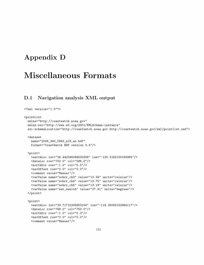
Appendix D
Miscellaneous Formats
D.1 Navigation analysis XML output
<?xml version="1.0"?>
<pointListxmlns="http://coastwatch.noaa.gov"xmlns:xsi="http://www.w3.org/2001/XMLSchema-instance"xsi:schemaLocation="http://coastwatch.noaa.gov http://coastwatch.noaa.gov/xml/pointlist.xsd">
<datasetname="2006_340_0942_n18_ws.hdf"format="CoastWatch HDF version 3.4"/>
<point><earthLoc lat="34.442345084532306" lon="-120.5162100165965"/><dataLoc row="702.0" col="586.0"/><northDir row="-1.0" col="0.0"/><navOffset row="0.0" col="0.0"/><comment value="Manual"/><varValue name="avhrr_ch3" value="13.34" units="celsius"/><varValue name="avhrr_ch4" value="13.75" units="celsius"/><varValue name="avhrr_ch5" value="13.19" units="celsius"/><varValue name="sat_zenith" value="27.41" units="degrees"/>
</point>
<point><earthLoc lat="33.71715205953104" lon="-118.35055152964117"/><dataLoc row="768.0" col="750.0"/><northDir row="-1.0" col="0.0"/><navOffset row="0.0" col="0.0"/><comment value="Manual"/>
151

152 APPENDIX D. MISCELLANEOUS FORMATS
<varValue name="avhrr_ch3" value="13.66" units="celsius"/><varValue name="avhrr_ch4" value="13.38" units="celsius"/><varValue name="avhrr_ch5" value="13.32" units="celsius"/><varValue name="sat_zenith" value="12.86" units="degrees"/>
</point>
<point><earthLoc lat="37.96232720746668" lon="-122.93276796240643"/><dataLoc row="373.0" col="403.0"/><northDir row="-1.0" col="0.0"/><navOffset row="0.0" col="0.0"/><comment value="Auto failed"/><varValue name="avhrr_ch3" value="10.77" units="celsius"/><varValue name="avhrr_ch4" value="11.06" units="celsius"/><varValue name="avhrr_ch5" value="10.36" units="celsius"/><varValue name="sat_zenith" value="43" units="degrees"/>
</point>
<point><earthLoc lat="32.67355292893255" lon="-117.21490134745726"/><dataLoc row="862.0" col="836.0"/><northDir row="-1.0" col="0.0"/><navOffset row="0.0" col="0.0"/><comment value="Auto OK"/><varValue name="avhrr_ch3" value="13.97" units="celsius"/><varValue name="avhrr_ch4" value="14.11" units="celsius"/><varValue name="avhrr_ch5" value="13.7" units="celsius"/><varValue name="sat_zenith" value="3.22" units="degrees"/>
</point>
<point><earthLoc lat="33.992583436357236" lon="-119.92197445615143"/><dataLoc row="743.0" col="631.0"/><northDir row="-1.0" col="0.0"/><navOffset row="0.0" col="0.0"/><comment value="Auto failed"/><varValue name="avhrr_ch3" value="12.17" units="celsius"/><varValue name="avhrr_ch4" value="12.4" units="celsius"/><varValue name="avhrr_ch5" value="11.91" units="celsius"/><varValue name="sat_zenith" value="23.27" units="degrees"/>
</point>
</pointList>

D.2. NAVIGATION ANALYSIS CSV OUTPUT 153
D.2 Navigation analysis CSV output
Note that long lines are wrapped and continuation lines indented. In the actual output, each point ison a single line.
"LAT","LON","ROW","COL","ROW_NORTH","COL_NORTH","ROW_OFFSET","COL_OFFSET","COMMENT","AVHRR_CH3","AVHRR_CH4","AVHRR_CH5","SAT_ZENITH"
34.442345084532306,-120.5162100165965,702.0,586.0,-1.0,0.0,0.0,0.0,"Manual",13.34,13.75,13.19,27.41
33.71715205953104,-118.35055152964117,768.0,750.0,-1.0,0.0,0.0,0.0,"Manual",13.66,13.38,13.32,12.86
37.96232720746668,-122.93276796240643,373.0,403.0,-1.0,0.0,0.0,0.0,"Auto failed",10.77,11.06,10.36,43
32.67355292893255,-117.21490134745726,862.0,836.0,-1.0,0.0,0.0,0.0,"Auto OK",13.97,14.11,13.7,3.22
33.992583436357236,-119.92197445615143,743.0,631.0,-1.0,0.0,0.0,0.0,"Auto failed",12.17,12.4,11.91,23.27
D.3 Color palette XML format
<?xml version="1.0" encoding="ISO-8859-1"?><!DOCTYPE palette SYSTEM "http://coastwatch.noaa.gov/xml/palette.dtd">
<palette name="HSL256" length="256"><color r="128" g="0" b="127" /><color r="125" g="3" b="130" /><color r="123" g="5" b="132" /><color r="120" g="8" b="135" /><color r="118" g="10" b="137" />
(... lines omitted ...)
<color r="140" g="12" b="0" /><color r="137" g="10" b="0" /><color r="135" g="7" b="0" /><color r="132" g="5" b="0" /><color r="130" g="2" b="0" /><color r="128" g="0" b="0" />
</palette>

154 APPENDIX D. MISCELLANEOUS FORMATS

Appendix E
AVHRR SST Product FAQ
This list of frequently asked questions is designed to answer some of the more in-depth user ques-tions received about AVHRR sea surface temperature products. The NOAA CLASS archive (http://www.class.noaa.gov) holds a long series of CoastWatch AVHRR SST products from 1990 to thepresent. The data is available in close to its original AVHRR LAC pixel resolution (1.1 km) in variousprojections depending on region including Mercator and polar stereographic. CoastWatch IMGMAP(.cwf) products are available prior to November 10, 2003 as a set of high/medium/low resolution regionswith various AVHRR channels, SST, cloud, and sensor angle data split into separate files for a givenAVHRR pass. CoastWatch HDF (.hdf) products are available from November 10, 2003 to the presentas high resolution regions with all AVHRR channel data, derived data, and angles in one file for a givenAVHRR pass. The questions and answers below deal with both CWF and HDF files.
E.1 Data formats and archiving
What are all the various categories of CoastWatch data files on CLASS?
There are many CoastWatch products on CLASS to search through – following is a guide to thecategories:
CW SWATHCoastWatch HDF capture station swath files produced starting November 10, 2003 to the present.The swath files contain data in the original AVHRR sensor scan projection before registration toa Mercator or polar stereographic map. Swath files are equivalent to NOAA 1b HRPT data butwith SST and cloud data computed, and AVHRR channels calibrated.
CW REGIONCoastWatch HDF regional node files produced starting November 10, 2003 to the present. EachHDF region file contains data from the swath files registered to a map projection.
CWALA, CWCAR, CWGRL, CWGOM, CWHAW, CWNOE, CWSOE, CWWECCWF files produced before November 10, 2003 for the Alaska, Caribbean, Great Lakes, Gulf ofMexico, Hawaii, Northeast, Southeast, and West Coast regions.
155

156 APPENDIX E. AVHRR SST PRODUCT FAQ
Why do I get all sorts of error messages when I run cwinfo with the -v option?
The -v option for the cwinfo tool tells it to print the status of file identification. The code steps througha number of file formats before it finds the one that works, prints the file information, and then exitswith a zero status code (zero indicates nothing went wrong). Leave off the -v option if you only wantto see normal output and no error messages. The tool prints the file identification tests as Java codeexceptions just as a convenience so that programmers can check the line numbers in the code for wherethe identification failed, which is good for debugging, but not intended for the average user.
When I run the CoastWatch tools on some files from CLASS, I get error messages. Isthere something wrong with the files?
We have had reports of data files obtained from the CLASS archive that are truncated or corrupt insome way. Users report that CoastWatch tools crash, report error messages, or simply don’t recognizethe file format. In some cases you can re-download the file and try accessing it again, because theerror occurred during transmission from CLASS to your local machine. CLASS can provided a digitalsignature file in order to check that the downloaded file was not corrupted during transmission (see theoptions in the CLASS shopping cart). In other cases, the files are corrupt in the archive itself, andshould be reported to CLASS as being invalid.
Not all the HDF files I access contain an SST or cloud variable. Why is that?
Some NOAA-12 data files covering Hawaii do not have SST and cloud computed because of a specialarrangement with Hawaii data users who wanted AVHRR channel data when no NOAA-12 operationalSST equation was available. There are also some NOAA-15 data files covering various US regions thatdo not have SST and cloud due to a processing system bug that was corrected by reprocessing the data(although some files were missed by the reprocessing). In general, all AVHRR SST products shouldcontain SST and cloud data. If they don’t, report the data file to CLASS.
Why does the graphics variable in some CWF files not have any data in it?
Some full regional panel CWF data files such as the ER region for the East Coast do not contain anygraphics data. This is due to a problem with the processing system for those files. There is a placeholderfor graphics data in CWF files which in some cases contains graphics for the smaller 512×512 CWFfiles, but in some larger region CWF files it contains all zeroes.
An easy way to create the missing graphics is to import a CWF SST file into HDF with cwimport(make sure to use --match sst so that the graphics aren’t imported as well) and run the cwgraphicstool on it to create and insert coast/land/grid graphics into the HDF file.

E.2. SST COMPUTATION 157
E.2 SST computation
Can I use the AVHRR SST products for front analysis?
CoastWatch AVHRR SST data can be used for SST front detection and is useful for small areas due toits relatively high spatial resolution. See the follow paper for one such front detection algorithm:
Ullman, D.S., and P.C. Cornillon, 2000: Evaluation of Front Detection Methods for Satellite-Derived SST Data Using In Situ Observations. J. Atmos. Oceanic Technol., 17, 1667-1675.
Why are there so many SST algorithms for the CWF data files on CLASS?
The different SST algorithms listed under “Datatype” on CLASS go hand-in-hand with the file namingconvention – each SST algorithm used has a different code as the last two characters before the .cwfextension. To search for any available SST, select all of the possible SST products. Generally only oneSST product will have been produced for a given satellite pass, but various algorithms have been usedover the time period of the CWF file production so they all appear in the Datatype check boxes.
The naming of the SST algorithms may be confusing for new users. “MCSST” stands for multi-channel but really any SST algorithm used by CoastWatch uses multiple channels to compute the SST.Sometimes SST is called ”moisture corrected” because that’s how all of the SST algorithms work – theygenerally use channel 4 and correct it for moisture in the atmosphere using thermal channel differenceterms (ch4 − ch5, ch3 − ch5, ch3 − ch4), either in a linear combination or non-linear combination. Themost accurate algorithm and coefficients to run at a given time is determined by NESDIS researcherswho call it the “operational algorithm” which changes from satellite to satellite and time period to timeperiod.
The results of an SST data search on CLASS should return a single SST product file per satellite passwhose data is SST – only advanced users comparing AVHRR channel data to SST results should beconcerned with which algorithm was used, or those who need to provide such details with a publication.
As an added note, CoastWatch HDF files are not searchable by SST algorithm because only one SSTalgorithm is available per region: the most accurate one according to comparison with buoy measure-ments. HDF products contain SST in the sst HDF variable, and the SST algorithm used is documentedby the sst equation attribute attached to the variable. Some older HDF files may be missing this at-tribute due to a bug in the processing software.
What happens when the solar terminator passes close to the center of a scene, which SSTalgorithm is used?
NOAA series polar orbiting satellites (for example NOAA-14, NOAA-15, NOAA-16 and so on) arelaunched into a sun synchronous polar orbit which results in the satellite passing over low and midlatitude regions at roughly the same time every day (as opposed to polar regions where it passes overevery 100 minutes). That time is initially set up to be once for daytime (sunlight hours) and once fornighttime (complete darkness). Some satellites such as NOAA-15 have slipped over time and pass overa region when the region is partially lit and partially dark because the sun has set and the satellite isviewing the solar terminator. In these cases, the SST algorithm used is switched between a daytimealgorithm and a nighttime algorithm depending on the sun angle at each pixel. For CoastWatch data,

158 APPENDIX E. AVHRR SST PRODUCT FAQ
either in CWF or HDF format, the algorithm is switched when the solar zenith angle is 85◦. Forsz ≤ 85◦, the pixel undergoes a daytime SST algorithm, and for sz > 85◦ a nighttime SST algorithm.Note that the cloud masking algorithm (mentioned below) uses a different threshold: 80◦ rather than85◦.
Why can I see a discontinuity in the SST values in some mixed day/night scenes?
See the question above. When the SST algorithm switches in the middle of a mixed day/night scene, theSST values computed often show a slight discontinuity at the threshold because the different algorithmsuse different coefficients and possibly use different thermal AVHRR channels. The discontinuity is morepronounced in cloudy data, data that should be masked anyway.
E.3 Cloud masking
What cloud mask tests were used for day and night scenes?
The cloud mask tests are different for day and night as follows:
DaytimeBit 1: Reflective Gross Cloud TestBit 2: Reflectance Uniformity TestBit 3: Reflectance Ratio Cloud TestBit 4: Channel 3 Albedo TestBit 5: Thermal Uniformity TestBit 6: Four Minus Five TestBit 7: Thermal Gross Cloud Test
NighttimeBit 1: Thermal Gross Cloud TestBit 2: Thermal Uniformity TestBit 3: Uniform Low Stratus TestBit 4: Four Minus Five TestBit 5: Cirrus TestBit 6: Channel 3B Albedo Test (CLAVR-x, HDF only)Bit 7: Channel 3B Albedo Uniformity Test (CLAVR-x, HDF only)
where bit 1 is the least significant bit, and bit 8 is the most significant. The CWF data files use onlyCLAVR-1 cloud mask tests as described in:
Stowe, L.L., P.A. Davis, and E.P. McClain, 1999: Scientific Basis and Initial Evaluationof the CLAVR-1 Global Clear/Cloud Classification Algorithm for the Advanced Very HighResolution Radiometer. J. Atmos. Oceanic Technol., 16, 656-681.
The HDF files use mainly CLAVR-1 tests but also two CLAVR-x tests at night, described in:
Jelenak, A. and A.K. Heidinger: Validation of CLAVR-x cloud detection over ocean usingAVHRR GAC sea surface temperature. Proceedings of SPIE – Volume 5658 Applications

E.3. CLOUD MASKING 159
with Weather Satellites II, W. Paul Menzel, Toshiki Iwasaki, Editors, January 2005, pp.292-298.
and have modified versions of the RGCT, RUT, and RRCT during the day that take advantage ofCLAVR-x style thresholds rather than static thresholds for these tests.
What happens with the cloud mask when a scene contains the solar terminator?
For data users interested in SST masking, the intended use for the cloud mask data is that regardless ofscene time (day, night, or mixed day/night), the cloud mask should be treated as zero = clear, non-zero= cloudy. If a scene contains the solar terminator then the set of cloud mask tests is switched at asolar zenith angle of 80◦, but the zero/non-zero rule still applies. If you need more information aboutexactly which tests were used at each pixel, you can use the solar zenith angle data for the pixel. Forsz ≤ 80◦, the pixel has daytime cloud mask tests, and for sz > 80◦ it has nighttime tests (although seethe answer to the next question below about cloud test bit mixing).
The CWF and HDF files have the same behaviour with respect to cloud mask test switching. TheHDF files always contain the solar zenith angle data for day or mixed day/night scenes, but are missingthe solar zenith angle for night scenes to decrease the file size, and because solar zenith angle data islargely useless at night. CWF SST and cloud mask data files may in some cases be accompanied bycorresponding solar zenith angle files (datatype ZA on CLASS) but not always as their production wasbased on the data requirements at the time. In most cases the scene time of CWF files and hence whichset of cloud mask tests were used can be determined from the scene time output line from the cwinfotool.
Why can I see a discontinuity in the cloud mask data in some mixed day/night scenes?
See the question above for a partial explanation. A different set of cloud mask tests are used for daypixels versus night pixels, so the cloud mask data pixels have different bits set depending on which sideof the discontinuity they lie. There is no one-to-one correspondence between day and night cloud tests.
In addition to a cloud mask data discontinuity at the solar zenith, in some cases the change from dayto night tests is not “clean”, rather there are some pixels on the day side of the sz = 80◦ line thatappear to have bits set the same as the night side of the line and vice-versa. There are two issues thatcontribute to this:
1. The solar zenith angles are rounded to the nearest 1/100th of a degree when written to an HDF file(or either 1/100th or 1/128th for a CWF file depending on the compression used) so a few pixelswith values of, for example, 80.003◦ will be rounded down to 80◦ even though they underwentprocessing with the nighttime cloud tests.
2. The cloud tests in some cases use neighborhood functions. The uniformity tests use a 2×2 boxof data pixels to the right and below a given pixel in the array to check for a condition beingtrue, and the result of the uniformity test flags all pixels in the 2×2 box with the test results,regardless of whether all those pixels are day or night. Both day and night have uniformity tests,so the results of uniformity tests at the day/night boundary are mixed. The mixing is generallyacceptable because the results are intended to be used for SST masking, not cloud type evaluationand the mixing only occurs in cloudy conditions, not clear SST conditions.

160 APPENDIX E. AVHRR SST PRODUCT FAQ
E.4 Navigation correction
What does navigation correction actually do, rewrite all the data in the file?
No, it only adds metadata to the file header to advise the CoastWatch Utilities software of how to readthe data. Think of navigation correction like this. The file metadata says “this file starts at a certainlatitude/longitude and has a certain number of rows, columns, and pixel size”. That metadata sets thephysical area for the file and cannot be changed by the navigation correction. Performing a navigationcorrection on the file sets up extra metadata in the header that says “for this variable (for exampleSST), when the user requests the pixel data at (0,0), give them the data from (0+x,0+y)” where x andy are the navigation correction offsets.
Have the CoastWatch products on CLASS been autonavigated to correct the coastlines,and if so how accurate is the navigation?
The CW REGION and CW SWATH files have been autonavigated, but the older CWF files listedunder other regional node categories have not. The autonavigation is accurate to ±1 pixel when it runssuccessfully, which is about 90% of the time. If navigation accuracy is a major concern, products shouldbe checked by hand and corrected if needed. Starting in 2007, both swath and mapped HDF productscontain two extra global HDF attributes to indicate the success/failure of the autonavigation algorithm:autonav performed which indicates true or false, and autonav quality which is an integer attributewritten when the autonavigation is successful to give an indication of the quality of the navigation aslow (0), medium (1), or high (2).
Was the cwautonav tool used for autonavigating the 2003 and later HDF files?
No, the CoastWatch data processing system for AVHRR uses the SeaSpace TeraScan software for auto-navigation, which employs a similar algorithm to cwautonav. The cwautonav tool was added to theCoastWatch software in 2004, mainly to aid users in working with the older CWF data files.
Is the autonavigation performed by the CoastWatch AVHRR processing system moreaccurate than cwautonav?
Yes, the best spatial accuracy is achieved by correcting navigation problems during HDF file productionrather than using cwautonav after production. The source of most navigation errors with NOAAsatellites is an inaccuracy in the on-board clock and an uncertainty in the roll of the satellite. Thoseerrors translate respectively to a shift in the scan line direction and sample direction when viewing theimage data in its original sensor scan geometry. The AVHRR processing system makes the correctionwhile in sensor scan geometry, and then registers the data to a map projection. Once in a mapprojection, you cannot correct the navigation perfectly using a simple x and y shift, except in smallareas. Generally CoastWatch regional data files cover only small areas of about 500-1000 km in radius,so correcting with an x and y shift works well enough in most cases.

E.4. NAVIGATION CORRECTION 161
How can I perform autonavigation of the pre-2003 CWF files?
The best way to perform navigation of CWF files is to import multiple CWF files to an HDF file withcwimport, then run the cwautonav tool on the new HDF file. That way, you only have to run thenavigation once and the results are applied to all the variables in the HDF file selected for navigation(see the question below about variables that should be navigated). Use the cwautonav command linetool with the default options. The key to successful autonavigation is to choose many navigation boxeswith feature-rich coastline segments (rather than a flat coastline with no curves). Use AVHRR visiblechannel 2 for navigation when possible, as channel 2 data provides the most contrast between land andwater. At night, you can fall back on AVHRR channel 4, channel 3, or SST since SST is very similarto channel 4.
After manually navigating a CoastWatch data file in CDAT, how can I access the naviga-tion offsets?
For CWF files that have been manually navigated, there is no way to extract the navigation metadatadirectly from the file using the most recent version (3.x) of the CoastWatch Utilities. You can use version2.3 of the package, by running the cwfatt tool (see the user’s guide in that version) and ask it to printthe horizontal shift and vertical shift attributes. You can then apply them to other CWF filesfrom the same date/time using the cwfnav tool (also in the version 2.3 package) as shown by example inthe user’s guide. Be careful about mixing version 2 (cwfnav) and version 3 (cwnavigate) command-linenavigation tools – they use different conventions for the navigation offset. A positive translation offsetin the version 2 tool is a negative translation offset in the version 3 tool and vice-versa. However oncethe offsets are set (using either the old or new tools), CDAT will know how to interpret them correctly.Note that navigating a CWF file and then converting to HDF to get the navigation metadata won’twork – when the import to HDF is done, the navigation is taken into account by shifting the imagedata, so the HDF file will not contain the navigation metadata.
For HDF files that have been manually navigated, you can extract the navigation metadata using thehdatt tool by asking for the nav affine attribute for a specific variable since HDF files stored navigationmetadata individually for each variable. See Appendix B for a description of HDF navigation metadata.An alternative to hdatt is the hdp command in the HDF Group software.
Why do the HDF files contain floating-point navigation corrections, but CWF files onlycontain integer corrections?
The floating-point values in the HDF files are a feature of the new file format. CWF files can onlycontain integer-valued translation offsets, where as HDF files can contain float-valued affine transformcoefficients which are much more flexible and can represent rotation, scale, shear, and translationtransformations. The CoastWatch Utilities software uses whatever offsets it can find in the file andconverts them internally to floats. When writing navigation corrections to CWF files, the translationoffsets are rounded to integers and an error occurs if the affine transform represents anything but asimple translation.

162 APPENDIX E. AVHRR SST PRODUCT FAQ
Should navigation corrections in CDAT, cwautonav, and cwnavigate be applied to allvariables in an HDF file?
No, only certain variables should have navigation corrections applied, namely those from the AVHRRsensor and sensor data derived variables. Graphics, solar zenith, satellite zenith, and relative azimuthangles should not be corrected. AVHRR channel data, SST, and cloud should be corrected. If you’reusing the command line tools, you can use the following option to match only the sensor type data:--match "avhrr ch.*|sst|cloud".
Are there any other autonavigation algorithms that I can use for CoastWatch data?
Randy Ferguson et. al. (NOAA, National Centers for Coastal Ocean Science, Center for CoastalFisheries and Habitat Research) have written a research paper on their experience with automaticregistration of daytime CoastWatch SST data:
Ferguson. R.L., C. Krouse, M. Patterson, and J.A. Hare. Automated Thematic Registration of NOAA,CoastWatch, and AVHRR Images. Photogrammetric Engineering & Remote Sensing. Vol. 72, No. 6,June 2006, pp. 677-685.
E.5 Map projections
What is the spheroid used for the CWF data files?
The answer is complicated. Running the cwinfo tool on a CWF file reveals that the files use a WGS-72spheroid which has a semi-major axis of 6378135 m and inverse flattening of 298.26. The reality is thatthe CWF files were registered to a Mercator or polar stereographic map projection using a sphere ofradius 6371200 m, but the NOAA 1b file (the source of the AVHRR data) used a WGS-72 spheroidfor the geographic coordinates with geodetic latitudes but the geodetic latitudes were not converted(datum shifted) to geocentric when the data was registered. If the data is regarded as having a sphericalearth model when imported into a GIS system, the coastlines at all points in the image are completelywrong in the north-south direction. However assuming WGS-72, you’ll find that if you match the centerpoints of the CWF files based on coastlines, the image data will match the coastlines reasonably wellexcept at the corners and edges where a 1-2 pixel error occurs.
Are the land mask and other graphics the same for all data files?
No. All the HDF files for a given region (for example the ER region) have the same land mask andgraphics in each file because they all cover the same physical area. However, when the switch fromCWF files to HDF files occurred in 2003, the map projections were upgraded to use a true WGS-84 spheroid rather than the mixed spheroid model as discussed above. Thus, CWF files all have aslightly different land mask and graphics data compared to their corresponding HDF files, because theyrepresent a slightly different physical area. This means that pixel (0,0) in a CWF file is not at the samelatitude/longitude as pixel (0,0) in the corresponding HDF file.

E.5. MAP PROJECTIONS 163
Which CWF file regions correspond most closely to the new HDF file regions?
The rough correspondence is as follows (note that some HDF regions have no corresponding CWFregion):
HDF region CWF node and regionAlaska North CWALA Northern AlaskaAlaska Sitka CWALA VancouverAlaska South CWALA Southern AlaskaAlaska West CWALA Western AlaskaCaribbean East CWCAR East Caribbean SynopticCaribbean West CWCAR West Caribbean SynopticEast Coast Bermuda noneEast Coast North CWNOE Full Regional PanelEast Coast South CWSOE Full Regional PanelGreat Barrier Reef noneGreat Lakes CWGRL Full Regional PanelGreat Salt Lake noneGulf of Mexico CWGOM Full Regional PanelHawaii CWHAW SynopticWest Coast Acapulco noneWest Coast Baja CWWEC Baja Mexico SynopticWest Coast North CWWEC NorthwestWest Coast South CWWEC Southwest
When converting the Alaska HDF products to an ArcGIS binary grid, why do I end upwith the data looking like it’s on the wrong side of the earth?
The CoastWatch HDF files and ArcGIS use different conventions for specifying the rotation angle ofthe central meridian. For the Alaska products, use the following projection string:
PROJCS[’WGS_1984_Stereographic_North_Pole’,GEOGCS[’GCS_WGS_1984’,DATUM[’D_WGS_1984’,SPHEROID[’WGS_1984’,6378137.0,298.257223563]],PRIMEM[’Greenwich’,0.0],UNIT[’Degree’,0.0174532925199433]
],PROJECTION[’Stereographic_North_Pole’],PARAMETER[’False_Easting’,<insert value>],PARAMETER[’False_Northing’,<insert value>],PARAMETER[’Central_Meridian’,<insert value>],PARAMETER[’Standard_Parallel_1’,60.0],UNIT[’Meter’,1.0]
]
and insert values for the central meridian, false easting, and false northing. The central meridian canbe determined from the center point longitude reported by running cwinfo -t, and the false easting

164 APPENDIX E. AVHRR SST PRODUCT FAQ
and northing can be computed from the .hdr file values for xllcorner and yllcorner as follows:[false east
false north
]=
[1− cos t − sin t
sin t 1− cos t
] [xllcorneryllcorner
]where t is the central meridian angle.

Appendix F
Acronyms
API Application Programming Interface
AVHRR Advanced Very High Resolution Radiometer
CDAT CoastWatch Data Analysis Tool
CLASS Comprehensive Large Array-data Stewardship System
CWF CoastWatch Format
DMG Disk Image
ESRI Environmental Systems Research Institute
FAQ Frequently Asked Question(s)
FY Feng Yun
GAC Global Area Coverage
GCTP General Cartographic Transformations Package
GeoTIFF Geographic Tagged Image File Format
GIF Graphics Interchange Format
GIS Geographic Information System
GMT Greenwich Mean Time or Generic Mapping Tools
GSHHS Global Self-consistent, Hierarchical, High-resolution Shorelines
GUI Graphical User Interface
HDF Hierarchical Data Format
HRPT High Resolution Picture Transmission
IDL Interactive Data Language
165

166 APPENDIX F. ACRONYMS
IMGMAP Image Map
JPEG Joint Picture Experts Group
JRE Java Runtime Environment
JNI Java Native Interface
LAC Local Area Coverage
MVISR Multichannel Visible and Infrared Scan Radiometer
NAD North American Datum
NCSA National Center for Supercomputing Applications
NDVI Normalized Difference Vegetation Index
NESDIS National Environmental Satellite, Data, and Information Service
NetCDF Network Common Data Form
NOAA National Oceanic and Atmospheric Administration
OPeNDAP Open-source Project for a Network Data Access Protocol
PDF Portable Document Format
PNG Portable Network Graphics
RGB Red/Green/Blue
SAA Satellite Active Archive (now part of CLASS)
SDS Scientific Data Set
SST Sea Surface Temperature
TDF TeraScan Data Format
THG The HDF Group
UTC Coordinated Universal Time
UTM Universal Transverse Mercator
WGS World Geodetic System
XML Extensible Markup Language
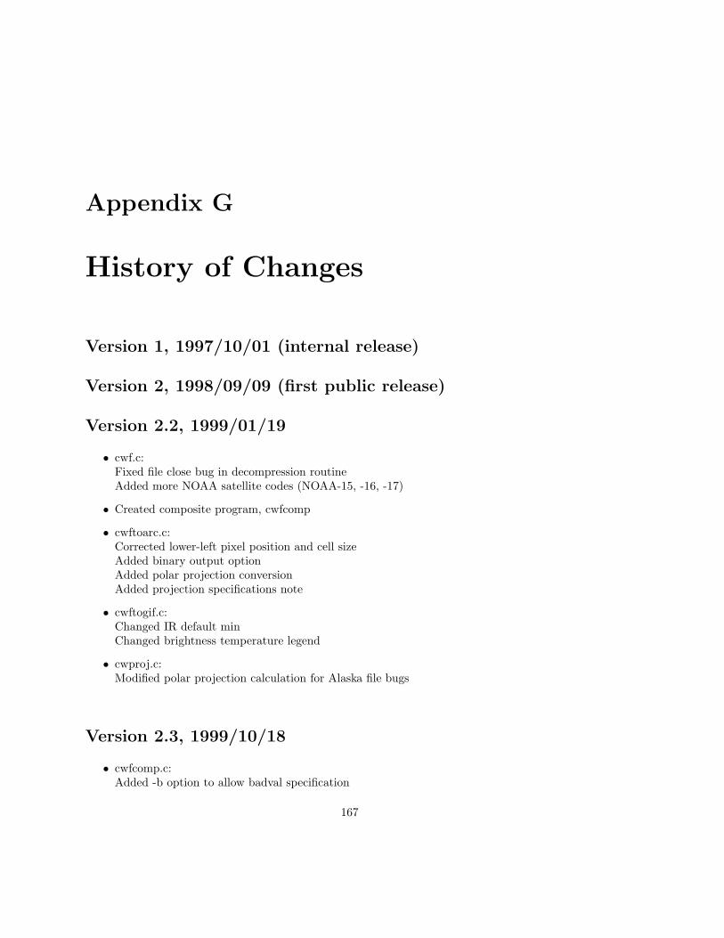
Appendix G
History of Changes
Version 1, 1997/10/01 (internal release)
Version 2, 1998/09/09 (first public release)
Version 2.2, 1999/01/19
• cwf.c:Fixed file close bug in decompression routineAdded more NOAA satellite codes (NOAA-15, -16, -17)
• Created composite program, cwfcomp
• cwftoarc.c:Corrected lower-left pixel position and cell sizeAdded binary output optionAdded polar projection conversionAdded projection specifications note
• cwftogif.c:Changed IR default minChanged brightness temperature legend
• cwproj.c:Modified polar projection calculation for Alaska file bugs
Version 2.3, 1999/10/18
• cwfcomp.c:Added -b option to allow badval specification
167

168 APPENDIX G. HISTORY OF CHANGES
Changed output file date to match last file
• cwf.c:Added f to various float constantsAdded test for near-zero IR valuesSimplified round functionFixed bug in cw compress for files with cols < 512Added calibration guess for older WCRN files
• cwfnav.c:Fixed usage message
• cwftogif.c cwftohdf.c cwftonc.c cwftoraw.c cwfval.c cwproj.c:Simplified round function
• cwproj.c:Added corrections for WCRN’s linear files
• cwftogif.c:Modified graphics plane layering, reformatted and commentedAdded ramsdis color palette for CH4 IR
• cwftohdf.c: Completely rewritten
• Created new HDF information routine: hdfinfo
• Created new landmasking routine, cwflmask
• Updated Makefile for new HDF and netCDF releases
Version 2.4, 2001/06/21 (internal release)
• Changed Makefile to include cwproj.c in libcwf.a
• Created cwflmaskdb routine
• cwproj.c: Modified for linear lat/lon header errors
• Fixed hdfinfo and cwftohdf usage messages
• cwf.c: Added orbit type “both” and channel number “sst multi”
• cwftohdf.c: Added orbit type “both” and channel number “sst multi”
• cwf.c: Added flat file support, reading only
• Moved cwftohdf to cwftocwhdf
• Moved hdfinfo to cwhdfinfo
• Fixed CWclone bug in hcwf library
• Added Julian day printing to cwhdfinfo

169
Version 3.1.0, 2001/07/19
• Implemented in Java using Java native interface to CWF and GCTP code.
• Now uses HDF4 via the HDF JNI calls.
• Now supports swath data.
Version 3.1.1, 2002/10/17
• Added rendering.
• Compiled shared libraries for Windows and Solaris.
Version 3.1.2, 2002/12/30
• Optimized coordinate translation code, rendering now runs 20% faster.
• Modified rendering normalization for viewable data only.
• Added grid overlay label drop shadows for better label legibility.
• Removed miter problems in shape drawings and coast lines.
• Added gridded dataset tile read/write caching for improved memory performance.
• Added NDVI palette.
• Corrected bitmask rendering for PDF files.
• Added registration tool for mapping between projections.
• Added generic bitmask rendering.
• Added navigation, master, sampling tools.
• Modified download tool command line parameters for regular expression matching.
• Added angle calculation tool.
• Improved coastline selection and rendering performance using binned GMT HDF dataset.
Version 3.1.3, 2003/03/31
• Added new tool for server status monitoring.
• Optimized download and status tools for database usage and updated command line options.
• Added GeoTIFF output for mapped projection data to cwrender.

170 APPENDIX G. HISTORY OF CHANGES
• Added NOAA 1b GAC/LAC AVHRR input.
• Fixed various bugs and made performance improvements.
• Updated Unix startup script for headless operations.
Version 3.1.4, 2003/05/16
• Added two new tools: cwmath and cwcomposite.
• Added MacOS X support in the dynamic JNI libraries and wrapper script.
• Fixed dateline crossing navigation problems in NOAA 1b readers – still needs refinement fornear-polar areas.
• Added basic GSHHS polygon rendering code to BinnedGSHHSReader – still needs refinement forbin boundaries and polygons broken by projection distortion.
• Added support for rendering progress to EarthDataView in preparation for CDAT operations.
• Added GLERL palettes “GLERL-Archive” and “GLERL-30-Degrees” palettes to the renderingtool and “NDVI” palette.
• Added “--age” option to download tool for specifying the desired maximum age of the data inhours.
• Added file chooser filters for “.hdf” and “.cwf” files in the cwmaster tool for easier use.
• Added 3D logos to rendering output.
Version 3.1.5, 2003/09/03
• Extended GeoTIFF output in cwrender to generate a paletted file when no overlays are used, andsuch that the ImageDescription TIFF tag contains a mapping equation from palette index to datavalue.
• Corrected cwimport so that the “pass type” attribute is correctly written when the metadataversion is < 3.
• Corrected the text output from cwexport to write “NaN” for invalid values.
• Corrected a 0.5 pixel offset problem in image overlay rendering.
• Added land polygon filling algorithms for cwmaster (by default) and cwrender (by using --coast).
• Added --operator option in cwstatus for verbose operator messages.
• Added bitwise or/and functions in cwmath.
• Added new “cwgraphics” tool to generate standard CoastWatch graphics overlays.
• Modified cwdownload to more gracefully handle connection errors and network timeouts.

171
Version 3.1.6, 2003/12/06
• Fixed space in resource path problem in Windows.
• Added support for AIX and IRIX.
• Added a resize bar for cwstatus between the online data list and data coverage / data previewpanels.
• Added the cwcoverage tool for showing region coverage plots (need to add ground station coveragecircle feature).
Version 3.1.7, 2004/06/19
• Updated TeraScan HDF import for equirectangular projections and spheroid detection.
• Changed EarthVectorReader to EarthVectorSource.
• Moved file path creation to IOServices.
• Created ContourGenerator and TopographyOverlay classes and added contouring to cwrender.
• Changed command line tools to split multi-parameter options on regular expression, including ’,’and ’/’.
• Added splash screen for cwmaster and cwstatus.
• Added support in CWHDFReader for explicit lat/lon data rather than polynomial coefficients.
• Changed use of Vector in many classes to ArrayList for better performance.
• Added support for unsigned HDF and CWF variable data.
• Modified data color scale in cwrender for better log scale behaviour.
• Modified cwmaster and cwstatus batch files to run with the Windows look and feel.
• Fixed automatic center calculation problem in cwcoverage.
• Fixed rounding problem in EarthDataViewPanel.TrackBar.
• Added build file for ant.
• Now using the Java install4j wizard to create installation packages.
• Re-coded and extended the CoastWatch Data Analysis Tool to work with the Java API. In additionto its 0.7a version, CDAT now has annotation and navigation capabilities, online help, GeoTIFFoutput, topography overlays, generic bitmask overlays, overlay groups, support for swath files,and more. CDAT is now an integrated part of the package.
• Modified the cwstatus menus to allow users to connect to a different server.
• Removed the cwrender preview option – it was causing problems with headless operations.

172 APPENDIX G. HISTORY OF CHANGES
• Updated online documentation in cwstatus and cwmaster.
• Replaced palette and RGB database files with XML versions.
• Added the --template option to cwmath so that users may use an existing variable as a templatefor the new variable rather than having to specify all of its properties.
• Added an update agent to graphical tools that informs the user if a software update is available.
Version 3.1.8, 2004/11/25
Updates
• Extended data caching in I/O routines to handle arbitrary size data arrays. Previously, someutilities would memory-thrash when faced with a large column count.
• Renamed various SatelliteXXX classes to EarthXXX to mirror more generality in metadata.
• Updated I/O for new metadata specifications, including multiple time periods and compositeattributes.
• Modified the default metadata version to 3.2. Now by default, new files created with the utilitiesare no longer compatible with the older CDAT version 0.7a and earlier.
• Updated coastline data files to GSHHS v1.3 and corrected known polygon fill problems on the USEast Coast, Africa, and South America.
• Updated ETOPO5 topography database and corrected problems with contours fills producingstrange bullseye artifacts.
• Added a --timeout option to cwdownload to allow the user to select a network timeout value.
• Added a --transform option to cwinfo to print Earth transform information.
• Modified the behaviour of cwcomposite to append dataset metadata together rather than simplyuse the last file’s global metadata (time, satellite, etc). The --pedantic option was also added toallow exact tracking of source dataset metadata.
• Added a --inputs option to cwcomposite to allow the user to specify a list of files in a text filerather than on the command line.
• Recompiled the HDF library for Linux to allow up to 256 open files. This allows the cwcompositeto handle more than 31 input datasets which was the previous limit.
• Modified cwmath to allow multiple input files, and output to an existing file that is not an inputfile.
• Updated to new install4j installation package wizard to fix various bugs and allow the user toselect components during a graphical installation.
• Added various option to cwcoverage tool for plotting ground station coverage circles.

173
Bug fixes
• Fixed stall problem in cwdownload when data server is unavailable or not responding within acertain timeout period.
• Fixed spelling problems with GCTP sinusoidal projection.
• Fixed swath reverse-lookup problems for non-AVHRR data.
• Fixed registration problems with partially swath-covered partitions in the output dataset.
• Fixed bitmask overlay navigation problem in CDAT.
• Fixed font problems in overlay group loading in CDAT on MacOS X.
• Fixed small polygons bug in CDAT coastline overlay.
• Fixed legend bounding rectangle line style problems in output from CDAT and cwrender.
• Fixed bitmask overlay rendering problems in CDAT on MacOS X.
• Fixed step color scale problems in image file output from CDAT.
• Fixed printing problems in cwinfo and cwstats.
• Fixed CDAT data view size change when many files are opened.
• Fixed CDAT data view so that if multiple file tabs are open and the user switches tabs, the dataview does not continue to render to the wrong tab.
• Fixed CDAT problem with allowing multiple overlay property control dialogs.
• Fixed CDAT problem with contour level deletion causing a stall.
• Fixed stall problems in CDAT related to delayed rendering.
• Fixed stall problems in cwstatus when server is not responding.
Version 3.1.9, 2004/04/07
Updates
• Updated NOAA 1b AVHRR reading for version 3 format.
• Added support in metadata and CW HDF reading/writing for sensor scan geometry geostationarysatellite data.
• Added LZW compressed GIF output for CDAT and cwrender.
• Added mixed resampling method to cwregister for handling discontinuities in the source data,such as in MODIS sensor data.
• Added cwautonav tool for estimating navigational corrections using image data.

174 APPENDIX G. HISTORY OF CHANGES
• Added transparent overlay color rendering in CDAT and cwrender, specifically for overlayinguser-specified polygon data without obscuring the background image.
• Modified graphical tools to output error messages that would normally go to the terminal to adialog. Now users will be able to see “uncaught” exceptions and decide to ignore them or file abug report.
• Added standard palettes specific to chlorophyll data.
• Added basic ESRI shapefile rendering support in CDAT and cwrender.
• Reformatted all tool manual pages and usage notes for clarity, as well as adding the equivalentone-letter options for all word-length options.
• Added general settings section in CDAT user preferences, initially for lat/lon format preferences.
• Modified all tools to clean up partially written data files after unexpected errors have occurred.
• Modified cwexport and cwrender to detect the desired file format based on the output file exten-sion.
• Added --nostates (don’t plot state border, just international borders) and --logo (plot a user-specified logo) options to cwrender.
• Added --imagecoords (print image row and column coordinates) to cwsample.
• Added log scale enhancements to CDAT.
• Updated graphical tool icons, menus, help pages, and Unix look-and-feel.
• Modified drop shadow rendering in CDAT and cwrender for better text readability.
• Added --projection option to cwdownload to allow the user to download only mapped or swathdata files.
Bug fixes
• Fixed overflow problem when writing HDF attribute data beyond 65535 values long.
• Fixed registration problem with navigationally corrected data.
• Fixed inappropriate missing value problem in ESRI ArcGIS grid and raw float output.
• Fixed “almost equals” problem with map projection parameter comparisons.
• Fixed background fill problem in CDAT data view when performing navigation.
• Fixed CDAT image saving bug; data view changed or became unusable after saving.
• Fixed problem with CDAT leaving files open even when user has closed file.
• Fixed PDF page size problem.

175
Version 3.2.0, 2005/10/08
Updates
• Added RasterPixelIsPoint style Earth location code for wind data.
• Improved speed of NOAA 1b reading by caching scan lines rather than tiles, as this reflects theactual file organization.
• Added support for OPeNDAP-accessible datasets with CoastWatch HDF metadata.
• Updated to perform datum shifting between Earth transforms of different datums.
• Changed “datum” terminology to “spheroid” in various locations.
• Added support for abstract GIS features to help in ESRI shapefile processing.
• Added spectrum and wind palettes for cwrender and CDAT.
• Added --limits option in cwstats.
• Added check for incompatible overlay group files in CDAT.
• Added support in cwrender for overlay group rendering, world files, vector data rendering, andunits conversion.
• Updated CDAT to have a special interface for opening OPeNDAP connections and datasets,moved file information to a full size window, and added 1:1 toolbar button.
• Added various detailed control options in cwautonav.
• Added hdatt tool for direct manipulation of HDF attribute information.
Bug fixes
• Corrected NOAA 1b longitude interpolation in polar regions.
• Modified to ignore coordinate variables in HDF files (for compliance with CF metadata conven-tions).
• Relaxed NOAA 1b format description check for varying descriptions in CLASS data files.
• Fixed unreliable convergence problem in swath Earth location reverse lookup algorithm.
• Fixed dropouts between rectangles in mixed resampling method for cwregister.
• Fixed Earth context element in output from cwrender to not draw coverage polygon when area islarger than orthographic projection area.
• Fixed problem with minimized window icons in graphical tools.
• Modified cwmaster so that map projections that support only sphere Earth models cannot besaved with an ellipsoid model.
• Modified the default locale for number formatting and printing to English/US to resolve problemswith inconsistent parsing of numbers formatted in other countries.

176 APPENDIX G. HISTORY OF CHANGES
Version 3.2.1, 2006/11/21
Updates
• Updated GUI code for better Mac OS X integration.
• Added help buttons in some areas of CDAT to aid users in getting context-specific help.
• Added color scale legend beside data view in CDAT in response to user suggestions.
• Added warning message in CDAT before applying navigation to make sure user understands thatthe data file is being modified.
• Changed “Save As” in CDAT to “Export” to avoid confusion. The data file should be thought ofas read-only and the save formats as export formats.
• Changed the order of operations for exporting data in CDAT to simplify the number of stepsusers need to perform.
• Added continuous enhancement updates in CDAT for visual appeal.
• Updated icons for data view controls in CDAT.
• Added drag-and-drop support in CDAT for opening data files.
• Updated all dialog box buttons in CDAT to more closely match platform defaults.
• Factored code for earth transforms to allow for both native C and Java map projection imple-mentations in the future.
• Added support in CDAT and cwrender for expression masking.
• Added support in CDAT for preferred units.
• Added support in CDAT and cwrender for saving image files with indexed 8-bit palettes.
• Added support in CDAT and cwrender for saving world files.
• Changed splash screen to not display by default for GUI tools. This was causing users to thinkthat startup was abnormally slow.
• Added support in NOAA 1b reading code for version 4 and 5 file formats, 8-bit and 16-bit sensorword sizes, MetOp data files, and files with missing scan lines.
• Added support for user file formats via the extensions/ directory.
• Added TIFF file compression in CDAT and cwrender.
• Added code for the Earth Data Access Client (EDAC) for for use by the CoastWatch East CoastNode (ECN).
• Added support in TeraScan HDF I/O code for importing a user-specified set of attributes.
• Updated GSHHS reading code to handle binned political line data, and replaced databases inTeraScan vector format with new HDF binned data from GMT. This speeds up the access andrendering of state and international lines considerably.
177
• Enhanced color scale in cwrender and CDAT to correctly show log scale ticks above the highestpower of ten on the scale. This helps with chlorophyll plotting when users scale between non-power-of-ten minimum and maximum.
• Added CDAT and cwrender palettes for Coral Reef Watch data.
• Added the --coherent option to cwcomposite based on CoastWatch central processing request. Seethe manual page for details.
• Updated look and content of application help files for CDAT, cwmaster, and cwstatus to be easierto read and navigate.
• Added ubyte/ushort types, and xor/not functions to cwmath.
• Added the --overwrite option to cwregister based on CoastWatch central processing request. Seethe manual page for details.
• Added the ability in cwrender to accept multiple --shape and --bitmask options. This makesrendering much more flexible.
• Added the --variable option to cwsample. It was confusing to users to have only --match and notbe able to depend on the ordering of columns in the output text file.
• Added the --region option to cwstats that takes a center point and radius for sampling.
• Modified the base directory for user preferences to be operating system specific. The base directorywas causing problems because different operating systems expect software to place customizationdirectories in different locations. See the help files in CDAT for the new locations.
• Standardized on [email protected] as the destination for all support emails.
Bug fixes
• Fixed error with log enhancement normalization by disabling the Normalize button for log en-hancements.
• Fixed status dialog problem in CDAT when loading variables with long names from files withshort names.
• Fixed color, stroke, and font swatch rendering in CDAT for Mac OS X.
• Fixed problem with writing ArcGIS files from CDAT and cwexport. Header file accuracy wasbeing impacted by writing to only two decimal places.
• Fixed problem when reading OPeNDAP files with 2D data of odd dimensions.
• Fixed error with retrieving chunks lengths while reading netCDF files, since netCDF has nochunking or compression support.
• Fixed null line color errors in CDAT overlays.
• Fixed problem with rendering text shadows for black grid lines in CDAT and cwrender.

178 APPENDIX G. HISTORY OF CHANGES
• Fixed problem with lat/lon separator characters in cwautonav. Now the documentation andimplementation match.
• Fixed cwdownload to delete partial files when a transfer error occurs.
• Fixed the lack of equation description in log-enhanced GeoTIFF output from cwrender and CDAT.
• Fixed error when working with geographic projection data that crosses the date line.
Version 3.2.2, 2007/11/06
Updates
Graphical tools
• Improved visibility of shape drawing in CDAT during zoom and annotation operations.
• Added full screen data view mode in CDAT.
• Added navigation analysis panel in CDAT.
• Added data reference grid overlays for drawing lines at regular image row and column spacings.
• Added a warning dialog in CDAT when navigation correction is about to modify a data file.
• Improved file open/save functionality in the CoastWatch Master Tool (cwmaster).
File formats and I/O
• Added support for reading NOAA/NESDIS AVHRR Clear-Sky Processor for Oceans (ACSPO)HDF data files.
• Modified ArcGIS binary grid header writer to include “nbits” value.
• Added support for reading NOAA 1b High Resolution Infrared Radiation Sounder (HIRS) datafrom NOAA KLMNN’ satellites.
• Modified CoastWatch HDF writing to handle writing explicit lat/lon values for earth locationdata.
• Modified netCDF file reading to handle data with greater than two dimensions as a set of 2Darrays.
• Added “scan time” variable to NOAA 1b file variables.
• Modified NOAA 1b file reading to read only the largest contiguous run of valid scan lines.
• Added support for reading erroneous NOAA-15 data files from CLASS that indicate the wrongfile version in the header.
• Added checks for spheroid compatibility in GCTP map projections.

179
Command line tools
• Added step sequential color palette for East Coast Node chlorophyll data.
• Added version printing option “--version” to all command line tools.
• Added the “--copy” option to cwimport so that entire variables can be copied from one file toanother.
• Added median value computation results to the output of the cwstats command.
Bug fixes
• Fixed problem with overlay groups not updating between CDAT tabs.
• Fixed problem with directory refresh on file open in CDAT.
• Fixed problems with box surveys in CDAT that were not correctly surveying very small boxes ofpixels.
• Fixed some problems with earth location reverse lookup in full orbit swath datasets.
Version 3.2.3, 2009/03/31
Updates
• Added support for NOAA 1b KLMN data files with AMSU-A, AMSU-B, and MHS sensor data.
• Added informational “Reading file information” message when opening large files in CDAT.
• Updated to use the netCDF Java library 2.2.22 for improved GRIB 2 file support.
• Improved expression parsing in cwmath to allow for symbol characters in variable names, such asminus signs.
• Added geometric mean composite and explicit command line ordering options in cwcompositetool.
• Added 64-bit IEEE floating point output option in cwangles tool.
• Created tool to automatically test command line tools and options (work in progress).
Bug fixes
• Corrected problem with reading CoastWatch HDF swath geolocation data. This was causing anerror when displaying or working with CoastWatch HDF swath projection data files.
• Regenerated HDF land mask files for use with autonavigation. The cwautonav tool was failingwhen encountering navigation points with latitude > 45 degrees.

180 APPENDIX G. HISTORY OF CHANGES
• Fixed problem with ACSPO HDF file buoy data variables being read and displayed in CDAT.
• Fixed problem with full orbit FRAC data files from Metop. Opening a full orbit file was resultingin a very long wait and CDAT becoming unresponsive.
• Fixed out of memory problems with opening and closing many large files in CDAT.
• Fixed unsupported file format error when reading TOVS data files with no archive header.
• Corrected ACSPO file I/O routines to read both orbit and granule metadata conventions.
• Corrected overflow error in cwdownload byte count for large file transfers.

Bibliography
[1] General Cartographic Transformation Package. http://edcwww.cr.usgs.gov/pub/software/gctpc.
[2] Global Self-consistent, Hierarchical, High-resolution Shoreline Database.http://www.ngdc.noaa.gov/mgg/shorelines/gshhs.html.
[3] Interactive Data Language. http://www.rsinc.com.
[4] Matlab. http://www.mathworks.com.
[5] NCSA HDF. http://hdf.ncsa.uiuc.edu.
[6] Open-source Project for a Network Data Access Protocol (OPeNDAP). http://www.opendap.org.
[7] Unidata UDUNITS package. http://my.unidata.ucar.edu/content/software/udunits/index.html.
[8] HDF Reference Manual, Version 4.1r2. University of Illinois at Urbana-Champaign, June 1998.
[9] HDF User’s Guide, Version 4.1r2. University of Illinois at Urbana-Champaign, June 1998.
181