coldwater reservoir ecology · 2014-01-08 · coldwater reservoir ecology federal aid project...
TRANSCRIPT

Coldwater Reservoir Ecology Federal Aid Project F-242-R15 Patrick J. Martinez Principal Investigator
Tom Remington, Director Federal Aid in Fish and Wildlife Restoration Job Progress Report Colorado Division of Wildlife Fish Research Section Fort Collins, Colorado May 2008

i
STATE OF COLORADO Bill Ritter, Governor COLORADO DEPARTMENT OF NATURAL RESOURCES Sherman Harris, Executive Director COLORADO DIVISION OF WILDLIFE Tom Remington, Director WILDLIFE COMMISSION
Tom Burke, Chair Claire M. O’Neal, Vice Chair Robert Bray, Secretary Dennis G. Buechler Brad Coors Jeffrey A. Crawford Tim Glenn Roy McAnally Richard Ray Harris Sherman John Stulp, Department of Agriculture
AQUATIC RESEARCH STAFF
Mark S. Jones, General Professional VI, Aquatic Wildlife Research Leader Arturo Avalos, Technician III, Research Hatchery Rosemary Black, Program Assistant I Stephen Brinkman, General Professional IV, F-243, Water Pollution Studies Harry Crockett, General Professional IV, Eastern Plains Native Fishes Matt Kondratieff, General Professional IV, Stream Habitat Restoration Patrick Martinez, General Professional V, F-242, Coldwater Reservoir Ecology & GOCO - Westslope Warmwater R. Barry Nehring, General Professional V, F-237, Stream Fisheries Investigations Kevin Rogers, General Professional IV, GOCO - Colorado Cutthroat Studies Phil Schler, Hatchery Technician V, Research Hatchery George Schisler, General Professional IV, F-394, Salmonid Disease Investigations Kevin Thompson, General Professional IV, F-427, Whirling Disease Habitat Interactions and
GOCO – Boreal Toad Harry Vermillion, Scientific Programmer/Analyst, F-239, Aquatic Data Analysis Nicole Vieira, Physical Scientist III, Water Quality Studies Paula Nichols, Federal Aid Coordinator

ii
Prepared by: ______________________________________________ Patrick J. Martinez, General Professional V Approved by: ______________________________________________ Mark S. Jones, Aquatic Wildlife Research Leader Date: _______________________________
The results of the research investigations contained in this report represent work of the authors and may or may not have been implemented as Division of Wildlife policy by the Director or the
Wildlife Commission.

iii
TABLE OF CONTENTS
Objective 1: Hydroacoustic Surveys of Kokanee and Piscivore Abundance in Existing and Proposed Broodwaters .................................................................. 1
Segment Objective 1: ........................................................................................................ 1 Introduction ................................................................................................................ 1 Methods and Materials .............................................................................................. 1 Results and Discussion ............................................................................................... 2 Objective 2: Population Demographics of Kokanee and Lake Trout and Others
Piscivores Threatening Kokanee ........................................................................ 3 Segment Objective 1: ........................................................................................................ 3 Introduction ................................................................................................................ 3 Methods and Materials .............................................................................................. 3 Results and Discussion ............................................................................................... 4 Segment Objective 2: ........................................................................................................ 4 Introduction, Methods, Results and Discussion ..................................................... 4 Objective 3: Zooplankton Composition and Density and Mysis Density in Selected
Waters .................................................................................................................... 4 Segment Objective 1: ....................................................................................................... 4 Introduction ................................................................................................................ 5 Methods and Materials .............................................................................................. 5 Results and Discussion ............................................................................................... 5 Segment Objective 2: ...................................................................................................... 17 Introduction .............................................................................................................. 17 Methods and Materials ............................................................................................ 17 Results and Discussion ............................................................................................. 17 Segment Objective 3: ...................................................................................................... 17 Segment Objective 4: ...................................................................................................... 17 Introduction, Methods, Results and Discussion ................................................... 17 Objective 4: Water and Otolith Microchemistry as a Forensic Tool to Trace and
Prosecute Illegal Movements of Fish ............................................................... 25 Segment Objective 1: ...................................................................................................... 25 Segment Objective 2: ...................................................................................................... 25 Introduction, Methods, Results and Discussion ................................................... 25 Objective 5: Technical and Cooperative Support in Other Research Investigations
and in Reservoir Management ......................................................................... 26 Segment Objective 1: ...................................................................................................... 26 Segment Objective 2: ...................................................................................................... 26 Introduction, Methods and Discussion .................................................................. 26 Literature Cited .................................................................................................................. 27

iv
Appendix A: Temperature and dissolved oxygen profiles, and Secchi depths measured in coldwater reservoirs in 2007 ....................................................... 28
Appendix B: Final Report: Forensic applications of otolith microchemistry for
tracking sources of illegally stocked whirling disease positive trout ........... 35 Appendix C: Powerpoint Presentation: Concepts, Concerns & Conflicts in the
Management of Native Fish Species & Nonnative Sport Fishes in the Western United States ....................................................................................... 90
Appendix D: Powerpoint Presentation; Invasive & Illicitly Introduced Aquatic
Species: Perspectived from the Upper Colorado River Basin ................... 110

v
LIST OF TABLES
Table 1. Crustacean zooplankton, excluding nauplii, densities (number per
liter) estimated from duplicate samples collected at three stations at Blue Mesa Reservoir on 01 June and 16 July, 2007. ..................................6
Table 2. Length frequency of crustacean zooplankton (measured to the nearest 0.1
mm) collected in Blue Mesa Reservoir on 01 June, 2007. Bl = Bosmina longirostris, D. ssp.= Unidentified daphnia species, Dbt = Diacyclops bicuspidatus thomasi, Dgm = Daphnia galeata mendotae, Dp = Daphnia pulex, Ln = Leptodiaptomus nudus. ..................................................................7
Table 3. Length frequency of crustacean zooplankton (measured to the
nearest 0.1 mm) collected in Blue Mesa Reservoir on 16 July, 2007. Bl = Bosmina longirostris, D. ssp.= Unidentified daphnia species, Dbt = Diacyclops bicuspidatus thomasi, Dgm = Daphnia galeata mendotae, Dp = Daphnia pulex, Ln = Leptodiaptomus nudus. ......................8
Table 4. Crustacean zooplankton, excluding nauplii, densities (number per
liter) estimated from duplicate samples collected at five stations at Dillon Reservoir on 18 July, 2007. ...................................................................9
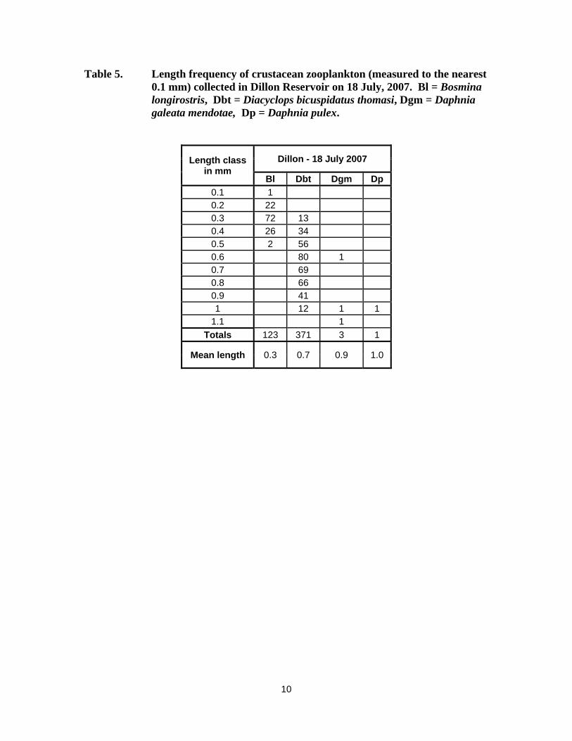
Table 5. Length frequency of crustacean zooplankton (measured to the
nearest 0.1 mm) collected in Dillon Reservoir on 18 July, 2007. Bl = Bosmina longirostris, Dbt = Diacyclops bicuspidatus thomasi, Dgm = Daphnia galeata mendotae, Dp = Daphnia pulex. ............................10
Table 6. Crustacean zooplankton, excluding nauplii, densities (number per
liter) estimated from duplicate samples collected at five stations at Granby Reservoir on 14 July, 2007. ..............................................................11
Table 7. Length frequency of crustacean zooplankton (measured to the nearest 0.1
mm) collected in Granby Reservoir on 14 July, 2007. Bl = Bosmina longirostris, Dbt = Diacyclops bicuspidatus thomasi, Dgm = Daphnia galeata mendotae, Dp = Daphnia pulex, Ln = Leptodiaptomus nudus. .......12
Table 8. Crustacean zooplankton, excluding nauplii, densities (number per liter)
estimated from duplicate samples collected at five stations at Taylor Park Reservoir on 17 July, 2007. ............................................................................13
Table 9. Length frequency of crustacean zooplankton (measured to the nearest 0.1
mm) collected in Taylor Park Reservoir on 17 July, 2007. Bl = Bosmina longirostris, Dbt = Diacyclops bicuspidatus thomasi, Dgm = Daphnia galeata mendotae, Dp = Daphnia pulex, Ln = Leptodiaptomus nudus, D. ssp.= Unidentified daphnia species. ...............................................................14

vi
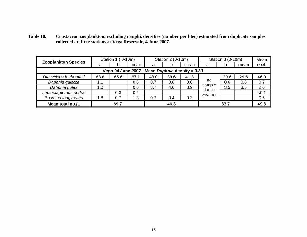
Table 10. Crustacean zooplankton, excluding nauplii, densities (number per liter) estimated from duplicate samples collected at three stations at Vega Reservoir, 4 June 2007. ...................................................................................15
Table 11. Length frequency of crustacean zooplankton (measured to the
nearest 0.1 mm) collected on Vega Reservoir, 4 June 2007. Dbt = Diacyclops bicuspidatus thomasi, Dgm = Daphnia galeata mendotae, Dp = Daphnia pulex, Bl = Bosmina longirostris. ...........................................16
Table 12. Summary of nighttime Mysis sampling at ten stations in Dillon
Reservoir on 17 July 2007, using vertical meter net (0.785m² bridle opening). Estimate of corrected lake wide mean Mysis density derived from duplicate samples at each station expressed as number per square meter. ..............................................................................18
Table 13. Mysis relicta length frequency for specimens collected from
nighttime vertical meter-net tows in Dillon Reservoir on 17 July 2007. Mysis total length in mm (tip of rostrum to tip of telson, excluding setae). ..............................................................................................19
Table 14. Summary of nighttime Mysis sampling at ten stations in Granby
Reservoir on 12 July 2007, using a vertical meter net (0.785 m² bridle opening). Estimate of corrected lake wide mean Mysis density derived from duplicate samples at each station expressed as number per square meter. .........................................................................20
Table 15. Mysis relicta length frequency for specimens collected from
nighttime vertical meter-net tows in Granby Reservoir on 23 August 2006. Mysis total length in mm (tip of rostrum to tip of telson, excluding setae) ...................................................................................21
Table 16. Summary of nighttime Mysis sampling at eight stations at aylor
Park Reservoir on 16 July 2007, using a vertical meter net (0.785 m² bridle opening). Estimate of corrected lake wide mean Mysis density derived from duplicate samples at each station expressed as number per square meter. No sample taken from Stations 3A and 3B due to shallow water depth. ...............................................................23
Table 17. Mysis relicta length frequency for specimens collected from
nighttime vertical meter-net tows in Taylor Park Reservoir on 16 July 2007. Mysis total length in mm (tip of rostrum to tip of telson, excluding setae). ..............................................................................................24

vii
LIST OF FIGURES
Figure 1. Comparison of estimated pelagic fish abundance in sonar surveys perfomed in Blue Mesa and Granby reservoirs, 1998-2007 ................................2
Figure 2. Mysis density and Daphnia biomass in Granby Reservoir, 1991-2007,
showing inverse relationship between these indices of mysid abundance and zooplankton prey for planktivourous kokanee. ......................22

1
State: Colorado Project No. F-242-R15 Title: Coldwater Reservoir Ecology Period Covered: July 1, 2007 to June 30, 2008 Principal Investigator: Patrick J. Martinez STUDY OBJECTIVE: To investigate factors which influence or might affect the
stability of sport fisheries in Colorado’s large (>1,000 surface acres), coldwater (>6,500 feet in elevation) reservoirs and to provide recommendations for the management and monitoring of these and similar reservoirs.
OBJECTIVE 1: HYDROACOUSTIC SURVEYS OF KOKANEE AND
PISCIVORE ABUNDANCE IN EXISTING AND PROPOSED BROODWATERS
Perform standardized hydroacoustic surveys to estimate pelagic fish abundance in established (Blue Mesa, Granby, McPhee, Vallecito,and Williams Fork) and proposed (e.g. Elevenmile and Green Mountain) kokanee brood stock waters, and in other reservoirs as resources allow. Segment Objective 1: Perform standardized sonar surveys at Blue Mesa and Granby
reservoirs.
INTRODUCTION The number of sonar surveys performed in 2007 was to be reduced to allow time for data analyses and manuscript preparation. In addition, zooplankton, Mysis, limnological profiles, and kokanee spawn run sampling and analyses were also be scaled back or suspended beginning in 2007 (Appendix A). At the request of biologists, several of the reservoirs surveyed by sonar in recent years were also surveyed in 2007 via cooperative assistance from this project. The results of these surveys are reported here. Sampling of kokanee spawn runs was not performed in 2007, however, some training was provided to allow this work to be continued by some biologists and their crews.
METHODS and MATERIALS Sonar surveys were performed on six reservoirs in 2007; about half the number performed in 2006 (Martinez 2007a). These included: Blue Mesa (7 and 8 August), Elevenmile (12 September), Granby (10 September), McPhee (14 August), Vallecito (13

2
August), and Williams Fork (11 September). Surveys were performed at night, and were scheduled around the dates of the new moon. A PC-controlled HTI 243 digital split-beam scientific echosounder with its 15o down-looking transducer mounted in towed vehicle and deployed using the apparatus described in Martinez (2005) was operated from a 22 foot Hewes SeaRunner powered by an 8-hp, four-stroke Yamaha outboard during the surveys. Standardized transects were followed using a Garmin 165 GPS. Data analysis was performed by Kevin Rogers, CDOW Aquatic Researcher.
RESULTS and DISCUSSION Numbers of pelagic fish estimated in sonar surveys of reservoirs in 2007 were: Blue Mesa, 299,883; Elevenmile 59,339; Granby, 213,214; McPhee, 273,849; Vallecito, 81,246; and Williams Fork, 80,694. Kevin Rogers adjusted survey data for selected reservoir transects in recent years to account for “noise” appearing in deep water strata (Martinez 2007). These adjusted data were used in Figure 1 to provide trends in estimated pelagic fish abundance in Blue Mesa and Granby reservoirs derived for sonar surveys.
0
200000
400000
600000
800000
1998 2000 2002 2004 2006 2008
Num
ber o
f pel
agic
fish Blue Mesa
Granby
Figure 1. Comparison of estimated pelagic fish abundance in sonar surveys
performed in Blue Mesa and Granby reservoirs, 1998-2007.

3
OBJECTIVE 2: POPULATION DEMOGRAPHICS OF KOKANEE AND LAKE TROUT AND OTHER PISCIVORES THREATENING KOKANEE
Survey key population demographics for kokanee (size and age at maturity) in established and potential brood stock waters and for lake trout and other piscivores (relative weight and growth rate) where they pose a threat to kokanee populations and their egg production (e.g. Blue Mesa and Granby). Segment Objective 1: Begin analysis of long-term data sets for kokanee spawn
runs to detect relationships among kokanee size, age or egg-production.
INTRODUCTION
The size and age structure of mature kokanee in Colorado’s fall spawn runs has
been examined in relation to trends in kokanee populations and egg production (Martinez 2004). Validation of kokanee ages determined by surface aging of otoliths is essential to accurately interpreting these population trends. Several methods of otolith age validation were presented and discussed at the CDOW Kokanee Workshop held on 13 February 2008 in Grand Junction.
METHODS and MATERIALS
The international standard for designating the birth date of fish in the Northern Hemisphere is January 1. Subsequent annuli, each denoting an increase in age of one year, are also assigned on January 1. Typically, any growth accrued prior to January 1 is denoted a “+”. Semelparous kokanee, which die following spawning in the autumn or winter, may not live until January 1 in their final year of life. Following convention, the ages of most mature kokanee sampled in the spawn runs at Colorado’s kokanee egg collection sites would be expressed according to the number of annuli, with a “+” indicating that portion of the otolith from the last annulus to the otolith edge, which represents fish’s final year of growth. This method of expressing kokanee ages led to considerable confusion in the past; therefore, ages of mature kokanee in Colorado are now expressed such that the otolith edge represents the end of somatic growth in the fish’s final year of life. Thus, a “3+” kokanee would be identified as an “age 4”, even if its natural death occurred before January 1. Three opportunities provided means of validating annuli of kokanee otoliths aged by surface examination without any preparation except removal of debris. The first involved the initial introduction of kokanee into McPhee Reservoir in 1988. This initial plant of kokanee fry had been treated with methyl testosterone to impart sterility and longevity with the goal of producing larger-than-normal kokanee. Kokanee > 400 mmTL from this plant sampled in 1993 and 1994 were confirmed to be age 6 and age 7, respectively, by examination of their otoliths. The second phase of validating annuli in the otoliths of mature kokanee resulted from the 1991 and 1992 plants of kokanee in

4
McPhee Reservoir. Mature kokanee averaging 369 mmTL captured in 1993 were determined to be age 3 based on examination of their otoliths. Similarly, mature kokanee averaging 366 mmTL captured in 1994 were determined to be either age 3 or age 4. Last, Martinez (2007) reported the ages of mature kokanee established following the marking of these cohorts as fry with feed-administered tetracycline at the Roaring Judy Hatchery.
RESULTS and DISCUSSION The confidence in the ages of mature kokanee facilitates further analyses of these data. Data from selected spawn runs will be utilized in conjunction with other data collected from these reservoirs for long-term analyses. Segment Objective 2: Prepare draft manuscript on lake trout management in
western U.S. incorporating input from co-authors and reviewers and submit to peer-reviewed outlet.
INTRODUCATION, METHODS, RESULTS and DISCUSSION A manuscript initially entitled Western Lake Trout Woes was drafted in 2007 and submitted to Fisheries for peer-review. Authors included myself, Patricia E. Bigelow (National Park Service, Yellowstone National Park, WY), Mark A. Deleray (Montana Fish, Wildlife & Parks, Kalispell, MT), Wade A. Fredenberg (U.S. Fish and Wildlife Service, Creston Fish and Wildlife Center, Kalispell, MT), Barry S. Hansen (Confederated Salish and Kootenai Tribes, Department of Natural Resources, Pablo, MT), Ned J. Horner (Idaho Department of Fish and Game, Coeur d’Alene, ID), Stafford K. Lehr (California Department of Fish and Game, Sacramento, CA), Roger W. Schneidervin (Utah Division of Wildlife Resources, Vernal, UT), Scott A. Tolentino (Utah Division of Wildlife Resources, Garden City, UT), and Art Viola (Washington Department of Fish and Wildlife, Wenatchee, WA). The manuscript is presently undergoing recommended revisions. OBJECTIVE 3: ZOOPLANKTON COMPOSITION AND DENSITY AND
MYSIS DENSITY IN SELECTED WATERS Estimate zooplankton composition and density in established and proposed kokanee brood sources, and Mysis density in reservoirs where they are an important food-web component (Granby, Taylor Park) and in other waters where Mysis have been introduced as resources allow. Segment Objective 1: Collect and analyze crustacean zooplankton and measure
temperature and dissolved oxygen at Blue Mesa and Granby reservoirs.

5
INTRODUCTION
Crustacean zooplankton monitoring has aided the understanding of trends in
reservoir food webs. Annual or periodic collection of zooplankton data has proven valuable in recommending management strategies for sport fisheries and kokanee egg production, particularly in reservoirs containing Mysis relicta.
METHODS and MATERIALS Crustacean zooplankton was sampled in five coldwater reservoirs in 2007. Blue Mesa was sampled on 1 June and 16 July, Dillon on 18 July, Granby on 14 July, Taylor Park on 17 July and Vega on 4 June. Zooplankton was sampled by oblique tows in the 0-10 stratum with a Clarke-Bumpus metered sampler (153 µm net). Samples were placed in 4 oz. Whirl-Pac bags and preserved in 70% ethanol. Processing of samples, zooplankter measurements and estimates of density were performed as described by Martinez (1992). Temperature and dissolved oxygen profiles were also measured on the dates of zooplankton sampling using a YSI Model-57 meter. Secchi depths were also measured to the nearest centimeter.
RESULTS and DISCUSSION Crustacean zooplankton densities and size structures from samples collected in coldwater reservoirs in 2006 are presented in Tables 1-9. Temperature, dissolved oxygen profiles, and Secchi depths measured on the dates of zooplankton sampling are provided in Appendix A.
Blue Mesa Reservoir had Daphnia densities of 5.8/L and 9.8/L when sampled in June and July, 2007 (Table 1). The Daphnia, particularly D. pulex, in these samples were large, averaging >1.0 mm (Tables 2 and 3). Daphnia in Dillon Reservoir were rare, <0.1Ll (Table 4), and small, <1.0 mm (Table 5), when sampled in July 2007. Granby Reservoir had a very low Daphnia density, 0.1/L, on 27 June (Table 27), despite epilimnetic temperatures exceeding 14-15oC (Appendix Table A-4). Taylor Park Reservoir had a moderate Daphnia density of 5.5/L on 17 July 2007 (Table 8), but the D. pulex in the sample were large, averaging 1.35 mm (Table 9). Surface waters exceeded 15o C at the time of sampling in 2007 (Appendix Table A-5. The Daphnia density in Vega Reservoir was low when sampled in early June, 2007, but D. pulex was dominant (Table 10) and the Daphnia were large, > 1.1 mm (Table 11).

6
Table 1. Crustacean zooplankton, excluding nauplii, densities (number per liter) estimated from duplicate samples collected at three stations at Blue Mesa Reservoir on 01 June and 16 July, 2007.
Zooplankton species Sapinero (0-10m) Cebolla (0-10m) Iola (0-10m) Mean
no./L a b mean a b mean a b mean Blue Mesa - 01 June 2007 - Mean Daphnia density = 5.8/L
Bosmina longirostris 2.2 3.5 2.9 17.9 18.2 18.1 20.7 21.7 21.2 14.0 Diacyclops bicuspidatus thomasi 5.1 7.8 6.5 4.9 4.7 4.8 2.3 3.6 3.0 4.7
Leptodiaptomus nudus 0.3 0.3 0.3 0.5 0.5 0.5 1.6 0.9 1.3 0.7 Daphnia galeata 0.8 0.7 0.8 0.7 2.5 1.6 1.9 1.1 1.5 1.3 Daphnia pulex 2.5 2.6 2.6 3.9 5.0 4.5 3.8 1.5 2.7 3.2
Unidentified Daphnia 1.8 2.0 1.9 0.5 1.1 0.8 0.7 1.5 1.1 1.3 Mean total no./L 14.8 30.2 30.7 25.2
Blue Mesa - 16 July 2007 - Mean Daphnia density = 9.8/L Bosmina longirostris 0.1 0.0 0.1 0.8 0.3 0.6 0.0 0.0 0.0 0.2
Diacyclops bicuspidatus thomasi 9.7 7.3 8.5 10.5 8.0 9.3 4.0 6.3 5.2 7.6 Leptodiaptomus nudus 4.0 1.8 2.9 3.9 4.4 4.2 8.8 13.2 11.0 6.0
Daphnia galeata 4.0 4.7 4.4 4.1 3.3 3.7 5.7 3.0 4.4 4.1 Daphnia pulex 6.0 5.8 5.9 5.3 3.4 4.4 2.8 3.1 3.0 4.4
Unidentified Daphnia 1.7 1.6 1.7 3.4 1.9 1.4 0.8 0.4 0.6 1.2 Mean total no./L 23.4 23.5 24.1 23.6

7
Table 2. Length frequency of crustacean zooplankton (measured to the nearest 0.1 mm) collected in Blue Mesa Reservoir on 01 June, 2007. Bl = Bosmina longirostris, D. ssp.= Unidentified daphnia species, Dbt = Diacyclops bicuspidatus thomasi, Dgm = Daphnia galeata mendotae, Dp = Daphnia pulex, Ln = Leptodiaptomus nudus.
Length class in mm
Blue Mesa – 01 June 2007
Bl Dp spp Dbt Dgm Dp Ln 0.2 15 1 0.3 80 3 0.4 38 6 1 0.5 13 5 6 0.6 14 22 3 0.7 11 31 6 2 0.8 1 7 40 24 1 0.9 3 22 24 1 7 19 21 1
1.1 1 4 23 2 1.2 1 4 14 2 1.3 2 9 1.4 1 11 1.5 9 1.6 2 1.7 3 1.8 2
Totals 146 1 59 152 151 8 Mean length 0.3 0.8 0.7 0.8 1.1 1.0

8
Table 3. Length frequency of crustacean zooplankton (measured to the nearest 0.1 mm) collected in Blue Mesa Reservoir on 16 July, 2007. Bl = Bosmina longirostris, D. ssp.= Unidentified daphnia species, Dbt = Diacyclops bicuspidatus thomasi, Dgm = Daphnia galeata mendotae, Dp = Daphnia pulex, Ln = Leptodiaptomus nudus.
Length class in mm
Blue Mesa – 16 July 2007
Bl Dp spp Dbt Dgm Dp Ln 0.2 3 0.3 1 8 1 0.4 17 10 0.5 28 34 0.6 15 9 0.7 2 8 1 1 6 0.8 16 6 6 7 0.9 3 4 7 4 1 1 13 6 4
1.1 1 1 1 17 24 3 1.2 1 13 14 4 1.3 1 21 22 2 1.4 2 9 9 2 1.5 11 7 1.6 1 9 13 1.7 2 2 1.8 9 2 1.9 1 3 1 2 5 2
2.1 3 2 2.2 2.3 1
Totals 2 9 100 127 118 86 Mean length 0.7 1.3 0.6 1.3 1.3 0.7

9
Table 4. Crustacean zooplankton, excluding nauplii, densities (number per liter) estimated from duplicate samples collected at five stations at Dillon Reservoir on 18 July, 2007.
Zooplankton species Station 1 (0-10m) Station 2 (0-10m) Station 3 (0-10m) Station 4 (0-10m) Station 5 (0-10m) Mean
no./L a b mean a b mean a b mean a b mean a b mean
Dillon - 18 July 2007 - Mean Daphnia density <0.1/L Bosmina longirostris 0.7 1.0 0.9 10.2 16.2 13.2 0.8 1.0 0.9 0.6 2.8 1.7 17.9 11.7 14.8 6.3
Diacyclops bicuspidatus thomasi 0.8 0.3 0.6 16.3 16.2 16.3 2.8 5.9 4.4 7.3 22.7 15.0 25.6 22.7 24.2 12.1
Leptodiaptomus nudus 0.1 <0.1 0.1 <0.1 <0.1 Daphnia galeata 0.1 <0.1 0.1 0.1 0.1 <0.1 Daphnia pulex 0.1 <0.1 <0.1
Mean total no./L 1.5 29.6 5.3 16.8 39.0 18.4
10
Table 5. Length frequency of crustacean zooplankton (measured to the nearest 0.1 mm) collected in Dillon Reservoir on 18 July, 2007. Bl = Bosmina longirostris, Dbt = Diacyclops bicuspidatus thomasi, Dgm = Daphnia galeata mendotae, Dp = Daphnia pulex.
Length class in mm
Dillon - 18 July 2007
Bl Dbt Dgm Dp 0.1 1 0.2 22 0.3 72 13 0.4 26 34 0.5 2 56 0.6 80 1 0.7 69 0.8 66 0.9 41 1 12 1 1
1.1 1 Totals 123 371 3 1
Mean length 0.3 0.7 0.9 1.0

11
Table 6. Crustacean zooplankton, excluding nauplii, densities (number per liter) estimated from duplicate samples collected at five stations at Granby Reservoir on 14 July, 2007.
Zooplankton species Station 1 (0-10m) Station 2 (0-10m) Station 3 (0-10m) Station 4 (0-10m) Station 5 (0-10m) Mean
no./L a b mean a b mean a b mean a b mean a b meanGranby- 14 July 2007 - Mean Daphnia density < 0.1/L
Bosmina longirostris 0.2 0.1 0.7 0.3 0.5 0.2 0.1 0.3 0.5 0.4 0.2 Diacyclops
bicuspidatus thomasi 51.8 73.0 62.4 43.4 31.9 37.7 65.1 43.5 54.3 18.1 72.8 45.5 40.9 31.5 36.2 47.2
Leptodiaptomus nudus 0.9 3.4 2.2 1.6 0.9 1.3 4.8 5.2 5.0 3.2 10.4 6.8 3.7 2.6 3.2 3.7 Daphnia galeata 0.4 0.2 <0.1 Daphnia pulex 0.2 0.1 <0.1
Mean total no./L 64.6 39.1 59.8 52.7 39.8 51.1

12
Table 7. Length frequency of crustacean zooplankton (measured to the nearest
0.1 mm) collected in Granby Reservoir on 14 July, 2007. Bl = Bosmina longirostris, Dbt = Diacyclops bicuspidatus thomasi, Dgm = Daphnia galeata mendotae, Dp = Daphnia pulex, Ln = Leptodiaptomus nudus.
Length class in mm
Granby - 14 July 2007
Bl Dbt Dgm Dp Ln 0.2 6 0.3 3 24 0.4 79 2 0.5 130 1 15 0.6 180 6 0.7 108 5 0.8 47 8 0.9 13 2 1 10 6
1.1 6 5 1.2 4 1.3 1 3 1.4 1 3 1.5 2 1.6 1.7 3
Totals 3 603 2 1 64 Mean length 0.3 0.6 1.0 1.3 0.9

13
Table 8. Crustacean zooplankton, excluding nauplii, densities (number per liter) estimated from duplicate samples collected at five stations at Taylor Park Reservoir on 17 July, 2007.
Zooplankton species Station 1 (0-10m) Station 2 (0-10m) Station 3 (0-10m) Station 4 (0-10m) Station 5 (0-10m) Mean
no./L a b mean a b mean a b mean a b mean a b mean Taylor Park- 17 July 2007 - Mean Daphnia density = 5.6/L
Bosmina longirostris 0.1 <0.1 <0.1 Diacyclops
bicuspidatus thomasi 18.4 18.0 18.2 15.0 35.2 25.1 13.8 43.2 28.5 42.1 39.7 40.9 26.2 24.7 25.5 27.6
Leptodiaptomus nudus 0.8 0.4 0.6 0.3 0.6 0.5 0.3 0.2 0.7 0.4 0.2 0.1 0.4 Daphnia galeata 1.5 1.3 1.4 0.2 0.1 0.2 1.8 1.0 1.5 1.0 1.3 0.4 0.6 0.5 0.9 Daphnia pulex 3.2 4.4 3.8 0.3 1.1 0.7 1.1 2.4 1.8 10.2 7.4 8.8 5.5 3.1 4.3 3.9
Unidentified Daphnia 1.2 0.9 1.1 0.1 0.1 <0.1 0.9 0.5 1.9 1.3 1.6 0.7 1.0 0.9 0.8 Mean total no./L 25.1 26.4 31.9 52.9 31.2 33.5

14
Table 9. Length frequency of crustacean zooplankton (measured to the nearest 0.1 mm) collected in Taylor Park Reservoir on 17 July, 2007. Bl = Bosmina longirostris, Dbt = Diacyclops bicuspidatus thomasi, Dgm = Daphnia galeata mendotae, Dp = Daphnia pulex, Ln = Leptodiaptomus nudus, D. ssp.= Unidentified daphnia species.
Length class in mm
Taylor Park - 17 July 2007
Bl Dbt Dgm Dp Ln D.- spp 0.1 0.2 0.3 1 23 1 0.4 55 1 0.5 93 1 0.6 128 2 2 0.7 104 6 2 2 0.8 57 20 17 1 0.9 17 4 9 2 1 3 1 18 1
1.1 13 1 1.2 9 1 1.3 1 10 1 1.4 1 1.5 1 12 1.6 4 1.7 2 1.8 3 11 1.9 4 2 12
2.1 9 2.2 4 2.3 3
Totals 1 480 38 142 7 5 Mean length 0.3 0.6 0.9 1.35 0.96 0.62
15
Table 10. Crustacean zooplankton, excluding nauplii, densities (number per liter) estimated from duplicate samples collected at three stations at Vega Reservoir, 4 June 2007.
Zooplankton Species Station 1 ( 0-10m) Station 2 (0-10m) Station 3 (0-10m) Mean no./L a b mean a b mean a b mean
Vega-04 June 2007 - Mean Daphnia density = 3.3/L Diacyclops b. thomasi 68.6 65.6 67.1 43.0 39.6 41.3
no sample due to
weather
29.6 29.6 46.0 Daphnia galeata 1.1 0.6 0.7 0.8 0.8 0.6 0.6 0.7 Dahpnia pulex 1.0 0.5 3.7 4.0 3.9 3.5 3.5 2.6
Leptodiaptomus nudus 0.3 0.2 <0.1 Bosmina longirostris 1.8 0.7 1.3 0.2 0.4 0.3 0.5
Mean total no./L 69.7 46.3 33.7 49.8

16
Table 11. Length frequency of crustacean zooplankton (measured to the nearest 0.1 mm) collected on Vega Reservoir, 4 June 2007. Dbt = Diacyclops bicuspidatus thomasi, Dgm = Daphnia galeata mendotae, Dp = Daphnia pulex, Bl = Bosmina longirostris.
Length
class in mm
Vega- 04 June 2007
Dbt Dgm Dp Bl 0.1 0.2 4 1 0.3 7 2 0.4 45 1 0.5 58 2 0.6 77 2 0.7 24 1 0.8 29 1 4 0.9 4 1 1.0 6 1 4 1.1 1.2 1.3 1 2 1.4 1 1.5 1 1.6 1 2 1.7 1 2
Totals 254 6 21 4 Mean length 0.62 1.27 1.1 0.4

17
Segment Objective 2: Sample Mysis in Granby and Taylor Park reservoirs.
INTRODUCTION Mysis prey on zooplankton, particularly Daphnia, and can be a complicating factor in reservoir fishery management. Periodic estimates of Mysis abundance allows fishery managers to understand or predict fishery trends in reservoirs or tailraces receiving entrained Mysis.
METHODS and MATERIALS Quantitative sampling for Mysis was performed on three reservoirs in 2007. Sampling was performed in Dillon on 17 July, in Granby on 12 July, and in Taylor Park on 16 July. Sampling was performed at night, near the date of the new moon. Samples were collected using a 1-m diameter x 3-m long conical net with 0.5 mm mesh lowered to the reservoir bottom at standardized stations located by GPS and retrieved at 0.37 m/s with an anchor windlass. Duplicate samples collected at each station were placed in 18 oz. Whirl-Pac bags, identified with a rag paper label, and preserved in 70% ethanol. In the lab, all samples were enumerated with one sample from each station being randomly chosen for measurement of individual mysids. Mysids were measured to the nearest millimeter from the tip of the rostrum to the tip of the telson, excluding setae.
RESULTS and DISCUSSION
Estimated Mysis densities and size structures for waters sampled in 2007 are given in Tables 12-17. Compared to the low estimated density of Mysis in Dillon Reservoir in 2006, 88.5/m2 (Martinez 2007), the density in 2007, 229/m2 (Table 12), indicates a rebound in the population. The 2007 sample contained some mysids > 15 mm (Table13), which were essentially absent in 2006 (Martinez 2007). Mysis in Granby Reservoir showed an increase from over 515/m2 in 2006 (Martinez 2007), to 1,185/m2 in 2007 (Table 14). Increasing or peak Mysis densities in Granby have been associated with declining or low biomass of Daphnia (Figure 2). The estimated density of Mysis in Taylor Park in 2007 was 470/m2 (Table 17). Segment Objective 3: Begin preparation of long-term summary of zooplankton data sets. Segment Objective 4: Begin analysis of long-term Mysis data sets.
INTRODUCTION, METHODS, RESULTS and DISCUSSION Segment Objectives 3 and 4 are discussed together here since the long-term examination of these data remains underway. For the zooplankton data set, efforts have included photographing representative specimens of each species detected in reservoirs sampled over the years by this project. For Mysis, long-term abundance data has been assembled to examine the relationship between sampling station depth and mysid abundance in comparison to reservoir depth at the time of sampling as an indicator of annual reservoir operations.

18
Table 12. Summary of nighttime Mysis sampling at ten stations in Dillon Reservoir on 17 July 2007, using vertical meter net (0.785m² bridle opening). Estimate of corrected lake wide mean Mysis density derived from duplicate samples at each station expressed as number per square meter.
Dillon - 17 July 2007 - 10 Stations - Mean Mysis/m² = 228.7
Sample number
Sampling stations ( water depth in meters) Data
summaryStratum I Stratum II Stratum III
1A - 51.8
1B- 52.9
2A- 33.5
2B- 38.5
2C- 35.1
2D- 36.6
3A- 9.4
3B- 11.2
3C- 17.6
3D- 12.8
#1 135 156 528 192 321 155 5 135 202 122 1951 #2 132 128 351 226 232 168 19 84 182 117 1639
Sum 267 284 879 418 553 323 24 219 384 239 3590 Mean 133.5 142 439.5 209 276.5 161.5 12 109.5 192 119.5 179.5

19
Table 13. Mysis relicta length frequency for specimens collected from nighttime vertical meter-net tows in Dillon Reservoir on 17 July 2007. Mysis total length in mm (tip of rostrum to tip of telson, excluding setae).
Dillon - 17 July 2007
Station -
sample #
Mysis length (mm) Totals
4 5 6 7 8 9 10 11 12 13 14 15 16 17 18 19 20 21 22
DN1A-2 3 17 23 33 18 12 6 1 5 6 4 3 1 132 DN1B-1 1 16 38 21 22 28 16 2 1 5 3 2 1 156 DN2A-1 1 4 33 77 97 89 123 83 8 1 1 3 6 1 1 528 DN2B-2 1 3 25 42 52 36 32 16 11 2 1 1 1 3 226 DN2C-2 5 8 11 64 65 37 18 10 7 3 1 3 232 DN2D-2 1 5 11 33 37 32 13 9 5 3 6 6 4 3 168 DN3B-1 1 5 20 18 34 34 19 4 135 DN3A-2 1 5 5 6 2 19 DN3C-2 7 32 44 48 36 10 5 182 DN3D-2 1 5 24 30 31 16 6 1 2 1 117 Totals 7 9 36 208 366 373 321 283 173 35 3 13 26 21 10 8 1 1 1895
Percent 0.37 0.5 1.9 11.0 19.3 19.7 16.9 14.9 9.1 1.8 0.2 0.7 1.4 1.1 0.5 0.4 <0.1 0.0 <0.1 100.0

20
Table 14. Summary of nighttime Mysis sampling at ten stations in Granby Reservoir on 12 July 2007, using a vertical meter net (0.785 m² bridle opening). Estimate of corrected lake wide mean Mysis density derived from duplicate samples at each station expressed as number per square meter.
Granby - 12 July 2007 - 10 Stations - Mean Mysis/m² = 1185.9
Sample number
Sampling stations ( water depth in meters) Data
summaryStratum I Stratum II Stratum III
1A- 52.6
1B- 49.6
2A- 28.8
2B- 22.7
2C- 30.8
2D- 22.7
3A- 17.1
3B- 11.7
3C- 15.5
3D-18.1
#1 3048 555 2029 225 581 519 800 410 483 605 9255 #2 2665 505 1603 829 359 336 816 328 679 1243 9363
Sum 5713 1060 3632 1054 940 855 1616 738 1162 1848 18618 Mean 2856.5 530 1816 527 470 427.5 808 369 581 924 930.9

21
Table 15. Mysis relicta length frequency for specimens collected from nighttime vertical meter-net tows in Granby Reservoir on 23 August 2006. Mysis total length in mm (tip of rostrum to tip of telson, excluding setae).
Granby 12 July 2007
Station - sample #
Mysis length (mm) Totals
4 5 6 7 8 9 10 11 12 13 14 15 16 17 18 19 20 21 GR1A-1 10 312 499 420 246 91 54 38 31 90 286 453 321 135 32 13 7 10 3048 GR1B-1 1 57 89 80 62 31 21 7 16 40 79 55 10 3 2 2 555 GR2A-2 4 76 277 292 213 88 82 34 12 30 109 203 107 59 9 6 2 1603 GR2B-1 2 4 19 34 23 28 20 15 7 7 16 18 17 6 5 3 1 225 GR2C-1 45 85 76 39 11 9 4 11 59 99 97 21 8 10 6 1 581 GR2D-1 3 25 79 101 90 61 53 31 8 8 16 27 8 7 1 1 519 GR3A-2 1 248 268 134 61 22 12 1 4 11 34 14 6 816 GR3B-2 2 102 120 60 22 10 4 1 1 2 3 1 328 GR3C-2 6 50 143 179 103 68 39 17 3 12 28 18 11 2 679 GR3D-1 9 59 161 146 69 51 33 18 6 16 18 17 1 1 605 Totals 38 533 1740 1522 928 461 327 166 99 275 688 903 502 221 59 31 11 10 8959
Percent 0.42 5.9 19.4 17.0 10.4 5.1 3.6 1.9 1.1 3.1 7.7 10.1 5.6 2.5 0.7 0.3 <0.1 <0.1 100.0

22
y/m
3
0
100
200
300
90 95 00 05 100
300
600
900
1200
1500Daphnia
Dap
hnia
µg
dry/
m3 Mysis
Mysis
no./ m2
Figure 2. Mysis density and Daphnia biomass in Granby Reservoir, 1991-2007, showing inverse relationship between these indices of mysid abundance and zooplankton prey for planktivourous kokanee.

23
Table 16. Summary of nighttime Mysis sampling at eight stations at Taylor Park Reservoir on 16 July 2007, using a vertical meter net (0.785 m² bridle opening). Estimate of corrected lake wide mean Mysis density derived from duplicate samples at each station expressed as number per square meter. No sample taken from Stations 3A and 3B due to shallow water depth.
Taylor Park - 16 July 2007 - 8 Stations - Mean Mysis/m² = 469.5
Sample number
Sampling stations ( water depth in meters) Data
summary Stratum I Stratum II Stratum III 1A- 38.3 1B- 40.2 2A- 26.7 2B- 28.7 2C- 18.4 2D- 22.4 3A- 3B- 3C- 11.9 3D- 9.9
#1 430 331 440 245 536 278 n/a n/a 539 502 3301 #2 564 303 280 375 242 203 n/a n/a 283 346 2596
Sum 994 634 720 620 778 481 n/a n/a 822 848 5897 Mean 497 317 360 310 389 240.5 n/a n/a 411 424 368.6

24
Table 17. Mysis relicta length frequency for specimens collected from nighttime vertical meter-net tows in Taylor Park
Reservoir on 16 July 2007. Mysis total length in mm (tip of rostrum to tip of telson, excluding setae).
Taylor Park – 16 July 2007
Station - sample #
Mysis length (mm) Totals
4 5 6 7 8 9 10 11 12 13 14 15 16 17 18 19 20 TY1A-1 4 14 20 51 77 89 66 20 3 6 15 24 25 12 4 430 TY1B-1 8 18 24 45 42 29 24 15 6 5 19 31 22 11 2 2 303 TY2A-1 1 3 13 40 59 74 91 48 16 2 10 23 34 21 4 1 440 TY2B-1 8 16 20 27 21 9 7 8 5 2 6 31 40 33 11 1 245 TY2C-1 6 50 71 57 53 36 31 21 15 12 61 78 31 11 3 536 TY2D-2 4 17 20 31 22 7 9 7 3 2 7 24 22 22 6 203 TY3C-2 2 15 32 50 60 50 45 18 4 2 2 3 283 TY3D-2 1 14 54 78 78 66 36 16 1 1 1 346 Totals 33 102 214 355 412 372 339 173 68 32 118 214 178 110 30 3 1 2786
Percent 1.18 3.7 7.7 12.7 14.8 13.4 12.2 6.2 2.4 1.1 4.2 7.7 6.4 3.9 1.1 0.1 <0.1 100.0

25
OBJECTIVE 4: WATER AND OTOLITH MICROCHEMISTRY AS A FORENSIC TOOL TO TRACE AND PROSECUTE ILLEGAL MOVEMENTS OF FISH
Initiate, facilitate and participate in water and otolith microchemical investigations to identify the utility of this technique as a potential forensic tool for tracing and combating illicit fish stocking by sampling at hatcheries (state, federal and private) and in select large reservoirs and their satellite waters. Segment Objective 1: Participate in finalization of hatchery water and otolith
microchemical study to assess forensic utility for tracking origins of diseased fishes.
Segment Objective 2: Participate in summarizing results, discussing feasibility
and recommending methodology of applying water and otolith microchemistry in forensic applications for law enforcement.
INTRODUCTION, METHODS, RESULTS and DISCUSSION
Segment Objectives 1 and 2 are discussed together here since the final documents
summarizing this research have been prepared or are being submitted for peer-review. Appendix B contains a final report entitled Forensic Applications of Otolith Microchemistry for Tracking Sources of Illegally Stocked Whirling Disease Positive Trout that was submitted to the submitted to the Whirling Disease Initiative, Montana Water Center. This report, authored by Dr. Brett M. Johnson, and Daniel Gibson-Reinemer of Colorado State University, myself, Dr. Dana Winkelman of the Colorado Cooperative Fish and Wildlife Research Unit, and Dr. Gregory Whitledge of Southern Illinois University in Carbondale, provides an “Eclectic Approach to Source Identification” to guide law enforcement in investigating cases in which otolith microchemistry could prove to be a valuable line of evidence. In addition, a manuscript developed from this research by Master’s student Dan Gibson-Reinemer entitled Elemental Signatures in Otoliths of Hatchery Trout: Distinctiveness and Utility for Detecting Origins and Movement has been submitted to Canadian Journal of Fisheries and Aquatic Science. Co-authors for this manuscript include Dr. Brett M. Johnson, myself, Dr. Dana L. Winkelman, Alan E. Koenig of the U.S. Geological Survey, Central Region Mineral Resources Team in Denver, Colorado, and Dr. Jon D. Woodhead, School of Earth Sciences, University of Melbourne in Australia.

26
OBJECTIVE 5: TECHNICAL AND COOPERATIVE SUPPORT IN OTHER RESEARCH INVESTIGATIONS AND IN RESERVOIR MANAGEMENT
Provide technical and cooperative support in other research investigations (e.g. strobes at Vallecito, yellow perch Perca flavescens in Blue Mesa) and in reservoir management including selecting angling regulations, fish stocking, and information dissemination, to help perpetuate fishery productivity and stability. Segment Objective 1: Participate in efforts to advance agency and public response
to combat illicit fish introductions in western Colorado. Segment Objective 2: Participate in dissemination of information, as needed or
feasible.
INTRODUCTION, METHODS and DISCUSSION
Segment Objectives 1 and 2 are discussed together here since several venues provided the opportunity to disseminate information regarding the growing problem of illicit fish introduction in western Colorado. Martinez (2007b) discussed the lack of a comprehensive strategy to control or combat the practice of illicit fish stocking by well-intentioned, inadvertent or malicious acts of individuals. Martinez (2006) described the potential large scale ecological consequences to both sport and native fishes due to basin-wide proliferation of illicitly introduced fishes. Fundamentally, to protect aquatic resources and to allow professional management strategies to prevail, the response to illicit fish introductions must shift from one ranging from acceptance and promotion to one of discouragement and prevention.
During this segment, I participated in four efforts directed at raising awareness and drawing attention to the expanding problem if illicit fish introductions in western Colorado. The first of these was in reviewing and commenting on a draft white paper by the Colorado Division of Wildlife to address Undesirable Aquatic Species Management. Next, I prepared a lecture for the Fishery Science (FW401) class at Colorado State University and presented it in November, 2007. This presentation entitled Concepts, Concerns & Conflicts in the Management of Native Fish Species & Nonnative Sport Fishes in the Western United States is provided in Appendix C. In March 2008, the Colorado-Wyoming Chapter of the American Fisheries Society organized and hosted a special session, “From Buckets to Bilge Pumps – Addressing the Spread of Exotic Fish and Organisms in Western Watersheds”, including a session on “Exotic Fish and Aquatic Nuisance Species”, in March 2008. I made a presentation, provided in Appendix D, entitled Invasive & Illicitly Introduced Aquatic Species: Perspectives from the Upper Colorado River Basin in the latter session. Last, I co-authored a manuscript with Dr. Brett Johnson and Dr. Arlinghouse of the Leibniz-Institute of Freshwater Ecology and Inland Fisheries in Berlin, Germany, entitled Are We Doing All We Can to Stem the Tide of Illegal Fish Introductions? for submission to a peer-reviewed outlet.

27
LITERATURE CITED Martinez, P. J. 1992. Coldwater reservoir ecology. Colorado Division of Wildlife, Federal Aid
in Fish and Wildlife Restoration Project #F-89, Job Progress Report, Fort Collins. 131 pp.
Martinez, P. J. 2004. Coldwater reservoir ecology. Colorado Division of Wildlife, Federal Aid
in Fish and Wildlife Restoration Project F-242-R11, Progress Report, Fort Collins. 122 pp.
Martinez, P. J. 2005. Coldwater reservoir ecology. Federal Aid in Fish and Wildlife
Restoration Project F-242-R12 Progress Report. Colorado Division of Wildlife, Fort Collins. 148 pp.
Martinez, P. J. 2006. Westslope warmwater fisheries. Great Outdoors Colorado Job Progress
Report. Colorado Division of Wildlife, Fort Collins. 125 pp. Martinez, P. J. 2007a. Coldwater reservoir ecology. Federal Aid in Fish and Wildlife
Restoration Project F-242-R14 Progress Report. Colorado Division of Wildlife, Fort Collins. 126 pp.
Martinez, P. J. 2007b. Westslope warmwater fisheries. Great Outdoors Colorado Job Progress
Report. Colorado Division of Wildlife, Fort Collins. 134 pp.

28
APPENDIX A
TEMPERATURE AND DISSOLVED OXYGEN PROFILES, AND SECCHI DEPTHS MEASURED IN COLDWATER
RESERVOIRS IN 2007
29
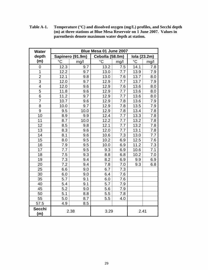
Table A-1. Temperature (°C) and dissolved oxygen (mg/L) profiles, and Secchi depth (m) at three stations at Blue Mesa Reservoir on 1 June 2007. Values in parenthesis denote maximum water depth at station.
Water depth
(m)
Blue Mesa 01 June 2007 Sapinero (91.9m) Cebolla (58.0m) Iola (23.2m)
°C mg/l °C mg/l °C mg/l 0 12.3 9.7 13.2 7.5 14.1 7.8 1 12.2 9.7 13.0 7.7 13.9 7.9 2 12.1 9.8 13.0 7.6 13.7 8.0 3 12.0 9.7 12.9 7.7 13.7 7.9 4 12.0 9.6 12.9 7.6 13.6 8.0 5 11.8 9.6 12.9 7.7 13.6 8.0 6 11.2 9.7 12.9 7.7 13.6 8.0 7 10.7 9.6 12.9 7.8 13.6 7.9 8 10.0 9.7 12.9 7.8 13.5 7.9 9 9.5 10.0 12.9 7.8 13.4 7.8 10 8.9 9.9 12.4 7.7 13.3 7.8 11 8.7 10.0 12.2 7.7 13.2 7.8 12 8.5 9.8 12.1 7.7 13.2 7.8 13 8.3 9.6 12.0 7.7 13.1 7.8 14 8.1 9.6 10.6 7.3 13.0 7.7 15 8.0 9.5 10.2 6.9 12.5 7.6 16 7.9 9.5 10.0 6.9 11.2 7.3 17 7.7 9.5 9.3 6.9 10.6 7.1 18 7.5 9.3 8.8 6.8 10.2 7.0 19 7.3 9.4 8.2 6.9 9.9 6.9 20 7.2 9.4 7.8 7.0 9.3 6.8 25 6.6 9.0 6.7 7.3 30 6.0 9.0 6.4 7.6 35 5.7 9.1 6.0 7.6 40 5.4 9.1 5.7 7.9 45 5.2 9.0 5.6 7.9 50 5.1 8.8 5.5 7.8 55 5.0 8.7 5.5 4.0
57.5 4.9 8.5 Secchi
(m) 2.38 3.29 2.41

30
Table A-2. Temperature (°C) and dissolved oxygen (mg/L) profiles, and Secchi depth (m) at three stations at Blue Mesa Reservoir on 16 July 2007. Values in parenthesis denote maximum water depth at station.
Water depth
(m)
Blue Mesa 16 July 2007 Sapinero (94.4m) Cebolla (57.5m) Iola (23.9m)
°C mg/l °C mg/l °C mg/l 0 20.8 6.4 20.9 5.4 21.9 5.4 1 20.2 6.4 20.3 5.5 20.4 5.5 2 19.8 6.2 20.0 5.6 20.2 5.6 3 19.7 6.1 19.9 5.6 20.0 5.7 4 19.6 6.1 19.8 5.6 19.9 5.8 5 19.5 6.1 19.8 5.6 19.8 5.7 6 19.3 6.1 19.7 5.7 19.5 5.6 7 18.8 6.2 19.6 5.7 19.2 5.6 8 17.6 6.0 19.5 5.6 18.8 5.6 9 16.0 6.0 16.4 5.0 17.7 5.4 10 15.5 6.0 15.8 4.8 16.7 5.3 11 14.8 6.0 15.4 4.6 15.6 5.0 12 14.3 6.1 14.6 5.0 15.2 4.8 13 13.6 6.1 14.0 5.0 14.8 4.8 14 13.3 6.0 13.6 5.0 14.9 4.6 15 12.9 6.0 13.3 5.0 13.6 4.3 16 12.4 6.0 12.6 12.6 13.0 4.2 17 12.0 6.0 12.2 12.2 12.5 4.0 18 11.7 6.1 11.8 11.8 12.1 4.0 19 11.1 6.1 11.6 11.6 11.8 3.9 20 10.7 6.1 11.6 11.6 11.4 3.8 25 9.0 6.5 9.1 9.1 30 7.8 6.7 7.8 7.8 35 7.0 6.8 7.0 7.0 40 6.5 6.8 6.6 6.6 45 6.1 6.8 6.2 6.2 50 5.9 6.8 6.1 6.1 55 5.6 6.9 5.9 5.9 58 5.5 7.0
Secchi (m) 7.20 8.57 5.69

31
Table A-3. Temperature (°C) and dissolved oxygen (mg/L) profiles, and Secchi depth (m) at five stations in Dillon Reservoir on 18 July in 2007. Values in parenthesis denote maximum water depth at station.
Water depth
(m)
Dillon 18 July 2007 P1 (66.7m) P2 (34.7m) P3 (24.0m) P4 (19.9m) P5 (13.1m) °C mg/l °C mg/l °C mg/l °C mg/l °C mg/l
0 16.1 6.7 16.3 6.1 16.1 6.0 16.8 6.1 17.5 6.1 1 16.1 6.5 16.4 6.1 16.1 6.2 16.7 6.1 17.4 6.1 2 16.1 6.3 16.3 6.1 16.1 6.1 16.4 6.2 17.0 6.1 3 16.1 6.3 16.3 6.2 16.0 6.1 16.3 6.2 16.7 6.2 4 16.0 6.4 16.0 6.2 16.0 6.2 16.1 6.1 15.9 6.3 5 16.0 6.4 15.8 6.2 15.9 6.1 15.3 6.3 15.7 6.3 6 16.0 6.3 14.0 6.3 15.2 6.2 14.9 6.3 15.4 6.3 7 14.3 6.4 13.9 6.4 15.1 6.2 14.1 6.3 15.2 6.2 8 12.7 6.5 12.2 6.5 13.1 6.3 13.2 6.3 13.4 6.3 9 11.0 6.6 11.6 6.6 12.1 6.4 11.9 6.4 12.2 6.3 10 10.6 6.7 11.2 6.6 10.8 6.4 11.7 6.4 11.7 6.2 11 9.9 6.7 11.1 6.6 10.2 6.5 10.7 6.5 10.9 6.3 12 9.7 6.6 10.6 6.6 9.6 6.5 9.9 6.4 9.7 6.2 13 9.3 6.6 10.2 6.6 9.2 6.5 9.5 6.4 9.5 6.1 14 9.0 6.6 9.7 6.6 8.9 6.5 9.3 6.3 15 8.7 6.6 9.5 6.6 8.6 6.5 9.1 6.3 16 8.3 6.6 9.0 6.5 8.5 6.5 8.9 6.3 17 8.0 6.6 8.6 6.5 8.3 6.5 8.3 6.3 18 7.8 6.6 8.4 6.5 8.1 6.5 8.2 6.2 19 7.5 6.6 8.2 6.5 7.8 6.4 7.8 6.1 20 7.2 6.7 7.7 6.5 7.5 6.5 25 6.3 6.8 6.6 6.7 30 5.7 6.9 6.2 6.7 35 5.3 6.9 40 5.0 6.8 45 4.8 6.8 50 4.6 6.8 55 4.5 6.7 59 4.4 6.6
Secchi (m) 3.43 3.06 3.08 3.39 3.16
32
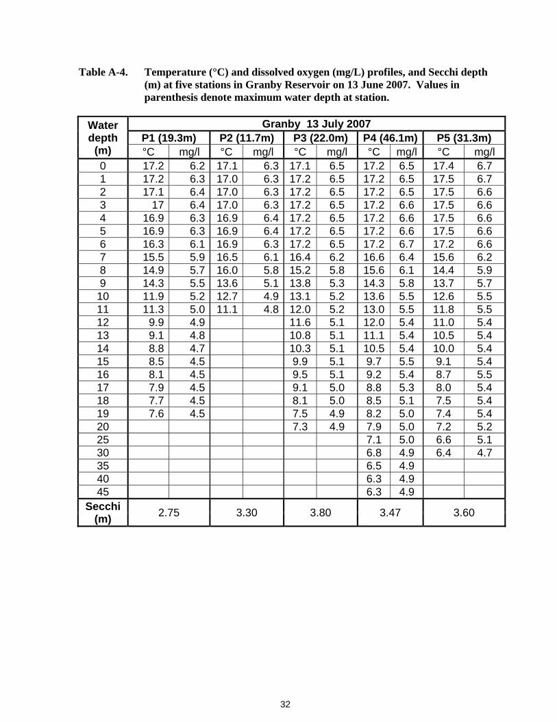
Table A-4. Temperature (°C) and dissolved oxygen (mg/L) profiles, and Secchi depth (m) at five stations in Granby Reservoir on 13 June 2007. Values in parenthesis denote maximum water depth at station.
Water depth
(m)
Granby 13 July 2007 P1 (19.3m) P2 (11.7m) P3 (22.0m) P4 (46.1m) P5 (31.3m) °C mg/l °C mg/l °C mg/l °C mg/l °C mg/l
0 17.2 6.2 17.1 6.3 17.1 6.5 17.2 6.5 17.4 6.7 1 17.2 6.3 17.0 6.3 17.2 6.5 17.2 6.5 17.5 6.7 2 17.1 6.4 17.0 6.3 17.2 6.5 17.2 6.5 17.5 6.6 3 17 6.4 17.0 6.3 17.2 6.5 17.2 6.6 17.5 6.6 4 16.9 6.3 16.9 6.4 17.2 6.5 17.2 6.6 17.5 6.6 5 16.9 6.3 16.9 6.4 17.2 6.5 17.2 6.6 17.5 6.6 6 16.3 6.1 16.9 6.3 17.2 6.5 17.2 6.7 17.2 6.6 7 15.5 5.9 16.5 6.1 16.4 6.2 16.6 6.4 15.6 6.2 8 14.9 5.7 16.0 5.8 15.2 5.8 15.6 6.1 14.4 5.9 9 14.3 5.5 13.6 5.1 13.8 5.3 14.3 5.8 13.7 5.7 10 11.9 5.2 12.7 4.9 13.1 5.2 13.6 5.5 12.6 5.5 11 11.3 5.0 11.1 4.8 12.0 5.2 13.0 5.5 11.8 5.5 12 9.9 4.9 11.6 5.1 12.0 5.4 11.0 5.4 13 9.1 4.8 10.8 5.1 11.1 5.4 10.5 5.4 14 8.8 4.7 10.3 5.1 10.5 5.4 10.0 5.4 15 8.5 4.5 9.9 5.1 9.7 5.5 9.1 5.4 16 8.1 4.5 9.5 5.1 9.2 5.4 8.7 5.5 17 7.9 4.5 9.1 5.0 8.8 5.3 8.0 5.4 18 7.7 4.5 8.1 5.0 8.5 5.1 7.5 5.4 19 7.6 4.5 7.5 4.9 8.2 5.0 7.4 5.4 20 7.3 4.9 7.9 5.0 7.2 5.2 25 7.1 5.0 6.6 5.1 30 6.8 4.9 6.4 4.7 35 6.5 4.9 40 6.3 4.9 45 6.3 4.9
Secchi (m) 2.75 3.30 3.80 3.47 3.60

33
Table A-5. Temperature (°C) and dissolved oxygen (mg/L) profiles, and Secchi depth
(m) at five stations on Taylor Park Reservoir on 17 July 2007. Values in parenthesis denote maximum water depth at station.
Water depth
(m)
Taylor Park 17 July 2007 P1 (12.8m) P2 (22.7m) P3 (33.6m) P4 (13.3m) P5 (11.4m) °C mg/l °C mg/l °C mg/l °C mg/l °C mg/l
0 17.0 6.6 16.8 6.6 16.9 6.4 16.9 6.4 17.5 6.31 16.7 6.7 16.8 6.6 16.9 6.4 16.8 6.5 16.6 6.52 16.6 6.7 16.7 6.6 16.8 6.6 16.6 6.5 16.5 6.53 16.6 6.7 16.7 6.6 16.7 6.6 16.3 6.5 16.3 6.54 16.5 6.7 16.6 6.6 16.5 6.5 16.2 6.5 16.3 6.55 15.4 6.7 15.8 6.7 16.0 6.6 16.1 6.6 16.1 6.66 15.0 6.6 15.1 6.7 15.5 6.5 16.1 6.6 16.0 6.67 14.8 6.7 13.2 6.7 14.6 6.4 16.0 6.6 15.8 6.68 14.1 6.7 12.3 6.6 13.2 6.7 14.0 6.4 15.1 6.49 13.4 6.8 12.0 6.4 12.5 6.7 13.5 6.1 14.0 6.310 12.4 6.6 11.0 6.0 11.6 6.5 12.8 6.0 13.2 6.211 11.5 6.1 10.8 5.8 11.1 6.2 12.3 5.9 12.8 6.112 10.8 5.6 10.5 5.8 10.9 6.0 12.1 5.8 13 10.2 5.8 10.6 5.8 11.7 5.8 14 10.0 5.8 10.3 5.6 15 9.8 5.8 9.8 5.6 16 9.5 5.8 9.4 5.7 17 9.3 5.9 9.2 5.4 18 9.0 5.9 9.0 5.4 19 8.8 5.9 8.9 5.4 20 8.7 5.8 8.7 5.4 25 8.0 5.6 30 7.8 5.5
Secchi (m) 6.66 6.01 5.68 5.67 6.40

34
Table A-6. Temperature (°C) and dissolved oxygen (mg/L) profiles, and Secchi depth (m) at three stations on Vega Reservoir on 27 July 2007. Values in parenthesis denote maximum water depth at station.
Water depth
(m)
Vega 27 July 2007 P1 (13.1m) P2 (18.4m) P3 (15.9m) °C mg/l °C mg/l °C mg/l
0 21.1 7.2 20.8 7.0 21.0 8.31 20.9 7.2 20.3 6.9 21.1 7.92 20.3 6.9 19.8 6.6 20.4 7.53 19.8 6.7 19.5 6.6 19.9 7.14 19.5 6.5 19.5 6.5 19.8 6.75 19.0 5.9 19.4 6.3 19.5 6.76 18.6 5.4 19.1 6.0 18.1 5.47 18.2 5.2 17.9 4.9 17.5 4.68 17.3 4.4 15.6 3.7 16.5 4.19 15.8 3.9 14.0 3.3 15.9 3.7
10 13.3 2.8 13.3 3.2 14.4 3.611 12.3 2.9 12.2 3.3 13.1 3.412 12.0 3.0 11.6 3.4 12.1 3.513 11.6 3.0 10.9 3.3 11.1 3.414 10.7 3.3 10.7 3.315 10.6 3.3 10.5 3.216 10.4 3.1 17 10.0 2.7 18 9.8 2.3
Secchi (m) 2.62 3.04 2.11

35
APPENDIX B
FINAL REPORT:
FORENSIC APPLICATIONS OF OTOLITH MICROCHEMISTRY FOR TRACKING SOURCES OF
ILLEGALLY STOCKED WHIRLING DISEASE POSITIVE TROUT

36
Final Report Reporting Period: August 2004 – June 2007
FORENSIC APPLICATIONS OF OTOLITH MICROCHEMISTRY FOR TRACKING SOURCES OF ILLEGALLY STOCKED WHIRLING DISEASE POSITIVE TROUT
Submitted to: Whirling Disease Initiative, Montana Water Center
Submitted by:
Dr. Brett M. Johnson, Professor Department of Fish, Wildlife and Conservation Biology, Colorado State University, 1474
Campus Delivery, Fort Collins, CO 80523-1474 Phone: (970) 491-5002; FAX: (970) 491-5091; Email: [email protected]
Daniel Gibson-Reinemer, Graduate Research Assistant Department of Fish, Wildlife and Conservation Biology, Colorado State University, 1474
Campus Delivery, Fort Collins, CO 80523-1474 Phone: (970) 491-2749; FAX: (970) 491-5091; Email: [email protected]
Patrick J. Martinez, Aquatic Researcher Aquatic Research Section, Colorado Division of Wildlife, 711 Independent Drive
Grand Junction, CO 81505 Phone: (970) 255-6141; FAX: (970) 255-6111; Email: [email protected]
Dr. Dana Winkelman, Professor and Leader Colorado Cooperative Fish and Wildlife Research Unit, 1474 Campus Delivery,
Colorado State University, Fort Collins, CO 80523-1474 Phone: (970) 491-1414; FAX: (970) 491-1413; Email: [email protected]
Dr. Gregory Whitledge, Assistant Professor Dept. of Zoology, Southern Illinois Univ., Carbondale, IL 62901-6501 Phone: (618) 453-7761; Fax: (618) 453-6095; E-mail: [email protected]

37
Abstract We used naturally occurring chemical markers to trace the environmental history
of hatchery trout. Analysis of water and otolith chemistry at hatcheries revealed a high
degree of temporal stability, coupled with high variation among hatcheries relative to
variation within hatcheries. Proportional relationships between water and otolith
chemistry for Sr:Ca, Ba:Ca, and 87Sr/86Sr allowed us to use these three quantities as
environmental markers in otoliths to classify trout to their hatchery of origin. Multivariate
models used to discriminate among hatcheries performed best when all three markers
were used, achieving an average accuracy of up to 96% for a group of five hatcheries.
Using only Sr:Ca and Ba:Ca, we were able to identify the hatchery of origin with
average accuracy rates which varied from 59% using a group of 11 hatcheries to 90%
when groups of only two hatcheries were considered. In a rigorous test of the forensic
capabilities of otolith chemistry, multivariate models classified a blind sample of at-large
fish stocked from hatcheries with 79% accuracy. Our results indicate the most effective
use of otolith chemistry in a forensic context will require collaboration with investigators
using traditional methods of inquiry to reduce the number of hatcheries classified with
otolith markers. We advocate an eclectic approach to source identification using
elemental and isotopic markers as a powerful new source of information that can be
used to strengthen cases based on multiple lines of evidence.
Introduction The maintenance of viable, self-sustaining wild trout fisheries is jeopardized by
the spread of whirling disease. Illegal stocking of whirling disease positive trout is
thought to be an important mode for introducing the disease into uninfected drainages
throughout the mountain west and Pacific Northwest. However, it has been virtually
impossible to identify where a fish originated from once it is released. Thus, it has been
extremely difficult for managers and law enforcement personnel to determine the
sources of such illegally stocked fish and prosecute individuals suspected of these
violations. The development of new technologies that identify sources would be an

38
invaluable law enforcement tool as well as a potent deterrent to discourage future
violations of this nature (Glenn Smith, CDOW Criminal Investigator, personal
communication).
Microchemical and stable isotope analysis of otoliths is emerging as an
extremely useful method for tracking origins and movement patterns, or provenance, of
fishes (Gao and Beamish 1999; Hobson 1999; Kennedy et al. 2000, 2002; Weber et al.
2002; Wells et al. 2003). Otoliths (“ear stones”, calcified structures of the inner ear used
in balance and hearing, Bond (1996)) have three properties that suit them to this kind of
analysis:
1) chemical constituents in water are passively absorbed by fish and deposited
in their otoliths. Some elements and their isotopes are deposited in the
otoliths in proportion to the environmental concentration, making them
excellent natural tracers (Campana and Thorrold 2001; Outridge et al. 2002).
2) Otoliths are physiologically inert, so once material is deposited it remains in
the otolith for the life of the fish. This is not true for most other parts or tissues
in a fish, which may be catabolized or otherwise lost or transformed.
3) Otoliths grow incrementally, even when the fish itself ceases to grow, in a
highly consistent manner. Thus, chemical information is deposited
chronologically.
Because water chemistry varies from place to place due to variations in lithology,
watershed characteristics, and land use and water use, otoliths of fishes from different
localities differ in their chemical composition. Further, fish that have moved among
locations of differing water chemistry carry a record of where and when they’ve
inhabited the various locations. Thus, otolith microchemisty offers considerable
promise as a means to track the origins of illegally stocked trout. Testing the utility of
the technique for this application was the focus of this research project.

39
Most of the research on otolith chemistry has been conducted with marine or
diadromous fishes (Campana 2005). However, freshwater systems have the potential
to display greater variation in key trace elements than the ocean (Campana et al. 1999),
allowing researchers to track environmental histories of fishes originating in
geochemically distinct areas. The chemical signatures in different freshwater
environments have proven to be useful tools for classifying fish to their location of origin
in areas as diverse as the Great Lakes (Ludsin et al. 2006), Arkansas (Bickford and
Hannigan, 2005) and Yellowstone National Park (Munro et al. 2005). Encouragingly,
freshwater systems have markers such as strontium (Sr) isotope ratios which are not
useful in marine environments but can be highly effective environmental tracers in
freshwater (Kennedy et al. 2002).
While otolith chemistry shows promise in freshwater systems, critical areas of
research need to be examined for it to become a valuable tool in forensic investigations.
The use of trace element signatures in otoliths to classify fish to locations in the
Mountain West has been accomplished in Wyoming (Munro et al. 2005) and Idaho
(Wells et al. 2003), but neither study examined otoliths from more than three locations
and both covered relatively small spatial scales. We anticipate investigations of illicit
stocking may involve more than three hatcheries and occur over broad spatial scales.
The classification accuracy of statistical models in such cases is a major factor in
determining how informative otolith chemistry will be. Additionally, no literature to date
has examined the variation in groundwater chemical signatures in the Mountain West.
The spread of whirling disease in wild rivers in the region has led a number of
hatcheries in Colorado to use groundwater sources to avoid contamination. Thus,
examining the variation in otolith chemistry among groundwater-fed hatcheries is a vital
step in determining the effectiveness of the technique for identifying sources of illicitly
stocked trout.
Our investigation was designed to fill in the gaps in the literature and to create a
template for forensic use of otolith chemistry. Prior studies have laid a substantial
foundation regarding the use of otolith chemistry, but the literature to date has not fully
investigated factors relevant to forensic applications of hatchery-reared fish in the
Mountain West. We expand upon the current state of the science with an investigation

40
which is novel in that we: examine variations in surface- and groundwater-fed
hatcheries; analyze variation in water and otolith chemistry over hundreds of miles; use
multivariate models to classify a number of locations unprecedented in freshwater
studies; and subject our data to a rigorous test simulating conditions which may exist in
a forensic case.
Materials and Methods We sampled water and fish from 17 CDOW trout hatcheries, one federal
hatchery, and two private hatcheries in Colorado, and one Wyoming Game and Fish
(WGF) hatchery during this study. The project originally intended to sample a range of
private facilities, but only two vendors agreed to participate in our study. To conserve
funds for other objectives and to make the best use of very limited instrument time, we
selected a subset of 16 CDOW hatcheries to use for water chemistry analyses and 11
CDOW hatcheries and one WGF hatchery to use for chemical analyses of otoliths
(Table 1). The hatcheries spanned a wide geographic and geologic range (Figure 1).
The maximum distance between pairs of hatcheries in Colorado was approximately 275
miles (Durango and Watson) and the minimum distance between pairs of hatcheries
was less than a mile (Bellvue and Watson).
We collected water from each hatchery in Colorado once per year. To maximize
our ability to examine temporal variation we collected samples in a different season
each year: summer in 2004, late winter in 2005, and fall in 2006, following the methods
of Shiller (2003). Because hatchery water supplies are usually well-mixed to insure that
gases are at atmospheric equilibrium, and analytical cost and precision are very high,
we collected a single sample per location in 2004 and 2005. In 2006 we collected 3 to 6
samples per location to verify our assumption about precision. We also collected 18
samples of hatchery feed consisting of six size categories representing two major feed
manufacturers from several CDOW, one private and one federal hatchery (Table 2) to
determine barium (Ba), strontium (Sr) and Sr isotope signatures (87Sr/86Sr). Water
chemistry and feed analyses were provided by the Center for Trace Analysis at the
University of Southern Mississippi using a Finnigan MAT Element 2 high-resolution
inductively coupled plasma mass spectrometer. Elemental concentrations were

41
normalized to calcium concentration because these ratios govern the biological uptake
of elements in otoliths (Campana 1999). The replicate samples collected in 2006 were
used to approximate sampling and analytical variance in previous years. Because
variance tended to increase with element:Ca ratios, we fit a linear regression to the
relationship and used that function to calculate estimates of error terms for water
chemistry in 2004 and 2005. Strontium:Ca, Ba:Ca, and 87Sr/86Sr were analyzed in a
multivariate analysis of variance (MANOVA) to test for significant differences among
locations, pooling data across years within a hatchery.
Approximately 10 rainbow trout (Oncorhynchus mykiss) or hybrids (O. mykiss x
O. clarki) were collected from each hatchery in summer 2004 and late winter 2005
(Table 3). In fall 2005, we collected ten rainbow trout from the Tillett Springs Fish
Hatchery in north central Wyoming. (Hereafter, fish collected directly from hatcheries
are referred to as “known origin fish”). At four hatcheries, fish were transferred as
fingerlings from one hatchery to another prior to collection (Table 4). In all other cases,
known origin fish had resided at the location from which they were collected since
hatching. We also collected a sample of 23 rainbow trout from Button Rock Reservoir
(BRR) on July 11, 2006; these fish had been stocked from the Bellvue hatchery as sub-
catchables (~3-5” TL).
To test the ability of otolith chemistry to identify the provenance of unknown
origin fish, we analyzed a blind sample of rainbow trout collected from the wild in 2004
by CDOW Researcher Kevin Thompson (Table 5). These samples were collected in
areas where CDOW had stocked rainbow trout and natural reproduction was
considered to be unlikely. Therefore, we were confident that all samples obtained in
this manner had originated in state hatcheries. (Hereafter, we refer to this sample as
“unknown origin fish.”) We received randomly numbered fish and a list of 8 hatcheries
from which they could have come; only four of those were the true sources. The 8
potential hatcheries of origin were among the 11 from which we chose to analyze
otoliths.
Sagittal otoliths were prepared as polished thin sections (Figure 2) following the
methods of (Whitledge et al. In Press). Right otoliths were embedded in epoxy and cut
transversely using a low speed saw with a diamond blade. Cut otolith sections were

42
sanded and polished down to the plane of the otolith core. Polished thin sections were
mounted on glass slides and cleaned with ultrapure water. We used laser ablation
inductively coupled plasma mass spectrometry (LA-ICP-MS) to collect data on the
elemental abundance of 24 elements in transects which were ablated along the axis of
growth from the otolith core to the edge. We were thus able to look for changes in the
chemical composition of the otolith over time and to separate distinct portions of the
otolith corresponding to different environmental signatures.
Otolith elemental analysis was provided by Alan Koenig at the USGS Mineral
Resources Laboratory in Lakewood, CO, with a Perkin Elmer ELAN6000 ICP-MS
coupled to a CETAC Technologies LSX-500 laser system. External calibration of the
system was conducted using a prototype USGS calcium carbonate reference material
MACS-1 (Steve Wilson, USGS, personal communication). This reference material is a
near matrix match for the aragonite in the otoliths. To control for the amount of otolith
ablated, elemental data were standardized relative to Ca. After standardization to Ca,
stable portions of transects were integrated to produce a mean concentration as in
Longerich et al. (1996) and reported as ppm. In cases where there was a change in the
chemical composition within an otolith, stable regions of each zone were integrated to
produce an average value while omitting the transition zones. The average values of
stable portions were used in multivariate analyses to characterize hatcheries.
Although usually composed of aragonite, sagittal otoliths in salmonids may also
contain portions of vaterite, an alternate crystal form of calcium carbonate. Vateritic
portions of otoliths have a different chemical composition from that of aragonite (Gauldie
1996; Melancon et al. 2005) and tend to occur with greater frequency in hatchery-reared
fish than in wild fish (Zhang et al. 1995; Bowen et al. 1999). We frequently encountered
vateritic portions of otoliths in our transect analyses and could identify them easily
based on the characteristically low levels of Sr and high levels of Mg (Gauldie 1996;
Melancon et al. 2005). The vateritic portions were excluded from our analyses because
they do not reflect the environment in the same fashion as aragonite.
Following analysis of elemental abundance, the 87Sr/86Sr ratio was analyzed in a
subset of otoliths by Dr. Jon Woodhead at the University of Melbourne. Otoliths were
cleaned to remove debris from the first ablation and subjected to a second ablation

43
along a transect parallel to that of the first ablation line using a Nu Plasma multicollector
inductively coupled plasma mass spectrometer. Time resolved scans of the 87Sr/86Sr
were processed by Alan Koenig and integrated over stable portions. Fish displaying
changes in 87Sr/86Sr over the transect were identified from the time resolved 87Sr/86Sr
ratios and average 87Sr/86Sr ratios were calculated for each region of the transect.
Discriminant function analysis (DFA) is a statistical method commonly used in
otolith studies to evaluate the extent to which distinct groups of fish have unique
chemical signatures and to identify group membership of specimens of unknown origin
(Wells et al. 2003, White and Ruttenberg 2006). Strontium and Ba were the only
elements which displayed a proportional relationship between otolith and water
chemistry and were the only elements used in multivariate models to classify known and
unknown origin fish. Isotope data were incorporated into models with Sr and Ba for a
smaller set of data. Both Sr and Ba were log transformed to meet the assumption of
homogeneity of variance (Levene’s test for homogeneity of variance p=0.216 and
p=0.586 for Sr and Ba, respectively). We used a cross-validated, leave-one-out
approach to classify otoliths of known origin fish (see Wells et al. 2003). There was no
significant year effect for Sr or Ba (ANOVA type 3 test of fixed effects, p=0.177 and
p=0.158 for Sr and Ba, respectively; Figure 3, so we pooled data from both years within
a location.
As the number of groups classified decreases, the accuracy of the models may
be expected to increase. To evaluate the increase in accuracy when number of groups
classified decreases, we performed additional analyses using subsets of two to ten
hatcheries from the pool of eleven known origin fish. Ten hatcheries were randomly
selected for each group size and analyzed in a DFA using Sr and Ba. On average,
random chance will classify fish correctly with a percentage inversely proportional to the
number of locations being classified and the performance of DFA models should be
compared to the accuracy expected due to random chance alone (White and
Ruttenberg, 2007).
To classify fish of unknown origin, we created a DFA model using the set of eight
suspected hatchery sources of the fish. This model was used to classify each of the
unknown origin fish to the most likely hatchery of origin. A separate DFA model was

44
constructed for the subset of otoliths for which both elemental abundance and isotope
data were collected.
Results and Discussion The near lack of private fish grower participation in our study had no negative
impact on our ability to test the utility of otolith chemistry for tracking provenance of
illicitly stocked trout. In retrospect, it was fortuitous that we used only government
hatcheries because they keep meticulous records of fish movements among locations
and have no incentive to withhold or provide misleading information regarding the
provenance of trout or their rearing practices. The range of geological and water
chemistry variation exhibited by the hatcheries included in our study provided an
excellent basis for evaluation of the technique. However, while the chemical signatures
we acquired form the foundation of a source database, signatures from private vendors
will be required in any future forensic application of otolith microchemistry.
Given the prohibitive costs associated with sampling water chemistry frequently,
we chose to stratify by season and collect water data over several years rather than
several times within a year. Because year was confounded with season in our sampling
design, and seasonal variation may actually exceed annual variation (John Stednick,
CSU Department of Forest, Rangeland and Watershed Stewarship, personal
communication) formal statistical tests of a year effect would be somewhat
inappropriate. Despite the inability to partition sampling variance, the variation of water
Sr:Ca and Ba:Ca ratios among hatcheries was large relative to variation within
hatcheries over time (Figure 4). A similar pattern emerged in 87Sr/86Sr ratio (Figure 5)
among hatchery water sources. Among hatcheries, the multivariate chemical signature
based on Sr:Ca, Ba:Ca, and 87Sr/86Sr ratio was highly significant (Pillai’s trace,
p<0.0001). Based on the patterns in water chemistry among hatcheries and the
significance of the MANOVA test, our evidence indicates that water chemistry remained
stable at a location over years relative to the differences among locations. This
conclusion is consistent with our findings from chemical analyses of otoliths. We had
only three years with which to examine interannual stability of hatchery water
signatures. However, a prolonged drought was temporarily alleviated in 2005 with near

45
normal runoff in many river basins in the state. This important interannual hydrologic
variation did not appear to obscure differences in chemical signatures among the
hatcheries.
The significant difference among hatchery water sources is exciting because of
the proportional relationship between water and otolith chemistry in freshwater
environments. Strontium:Ca ratios in otoliths of hatchery-resident trout varied in
proportion to the ratios in the hatchery water sources (Figure 6). Barium:Ca ratios in
hatchery-resident trout otoliths tended to display greater within-site variation but also
increased with increasing Ba:Ca ratios in water sources (Figure 6). Both Sr:Ca and
Ba:Ca display positive relationships between water and otoliths, as expected based on
other freshwater otolith studies (Wells et al. 2003; De Vries et al. 2005). No other
element we examined showed a discernable relationship between water and otoliths.
This finding is also consistent with other freshwater studies which have not yet
demonstrated conclusive evidence linking water and otolith concentrations of other
elements (as opposed to isotopes).
Our DFA models described the chemical composition or multivariate signature of
the otoliths from each hatchery. Chemical composition of individual otoliths can be
compared to the models and the otolith will be assigned to the hatchery to which it is
most similar. In a verification test of the DFA model using only Sr and Ba, otoliths from
the known origin fish from 11 hatcheries were assigned to their hatchery of origin with
59% accuracy (Table 6). While perhaps sounding unimpressive, given the relatively
large number of locations which were classified with only two elements, the results are
noteworthy. Limitations to the ability to classify fish on the basis of otolith signatures are
set by the variation in water chemistry signatures among locations and the variation
within otoliths from each location. In this case, the locations displayed a wide range of
otolith and water signatures, suggesting that the most effective way to increase the
accuracy of classification with Sr and Ba alone is to reduce the number of locations
classified. This is demonstrated in the simulation where we decreased the number of
hatcheries classified and average accuracy increased considerably beyond what was
achieved in a model with eleven hatcheries and was considerably higher than would be
expected due to chance alone (Figure 7).

46
We also performed a validation test of our DFA models using unknown origin
fish. This classification of unknown origin fish was a very rigorous challenge of the
capabilities of otolith chemistry. The model based on eight potential sources included
four “dummy” locations. Further, the unknown samples were otoliths from fish stocked
in 2003, while the known origin otoliths on which the model was based were collected in
2004 and 2005. Therefore, we simulated a situation where otolith data were used to
identify origins of fish stocked in previous years. Despite these obstacles, the model
displayed an overall success rate of 59% (Table 7). This level of success is a testament
to the stability of otolith signatures within a location over time as well as the stability of
otolith signatures in hatchery fish that have been at large for long periods of time. When
only the four true source hatcheries were included in a DFA model, the average
accuracy increased to 79%, again, highlighting the improvement of model performance
with smaller pools of candidate hatcheries.
Although Sr and Ba were the only elements that proved to be reliable markers,
strontium isotopes in otoliths were correlated with strontium isotopes in water (Figure 8.
We observed a departure from the expected 1:1 relationship between otolith and water,
however, which is consistent with other studies of hatchery fish. Otoliths of wild
diadromous fish tend to reflect the unadulterated isotopic ratio of the ambient water
(Kennedy et al. 2002; Woodhead et al. 2005), but the influence of marine-derived feed
appears to exert an influence on 87Sr/86Sr ratios in hatchery-reared salmonids (Ingram
and Weber 1999; Kennedy et al. 2002). Seawater has a globally constant 87Sr/86Sr
value of 0.709172 (Hodell et al. 1990), while freshwater systems have a range of values
above and below seawater levels (Graustein 1989). Hatchery-reared fish inhabiting
waters with 87Sr/86Sr ratios below seawater had otolith 87Sr/86Sr ratios higher than that of
the ambient water, while hatchery-reared fish inhabiting water with 87Sr/86Sr ratios
exceeding those of seawater had 87Sr/86Sr ratios in their otoliths lower than the ambient
water. The marine-derived feed appears to “pull” the otolith 87Sr/86Sr ratios towards the
seawater average without obscuring the ambient water values. Thus, the 87Sr/86Sr ratio
appears to be a valuable environmental marker for hatchery fish. Model accuracy
improved substantially with the addition of 87Sr/86Sr ratios. For the subset of five
hatcheries for which both elemental abundance and isotopic ratios were collected,

47
average accuracy rose from 63% using only Sr and Ba to 96% with the addition of
isotope data (Table 8).
Transects of otoliths from fish known to have moved between locations indicate 87Sr/86Sr ratios are more sensitive to movements than elemental abundances. In the
seven instances where we collected otoliths of fish that were moved from one hatchery
to another but resided at each location for more than one month, we observed
unequivocal shifts in elemental abundance in only one (TSP to TFH; Table 9). Many of
the unknown origin fish we collected also failed to show differences between the core
and edge portion, although we know they had moved. However, shifts in 87Sr/86Sr ratio
were clearly evident in the only two groups of fish for which 87Sr/86Sr data are available.
Twenty otoliths from BRR were analyzed for elemental abundance, and a subset
of five was analyzed for 87Sr/86Sr. In 11 of 19 elemental transects, we were able to
observe distinct core and edge signatures corresponding to the material deposited at
Bellvue Hatchery and BRR, respectively. Transects of 87Sr/86Sr were more revealing,
distinguishing the core and edge signatures in all five otoliths analyzed; transects of
elemental abundance for these same five otoliths only revealed core and edge
signatures in two cases. Thus, we believe 87Sr/86Sr analysis was the most effective
means to discern movement between locations in our study area, as elemental
abundance transects often failed to detect movements which are known to have
occurred.
Failure to detect movement is likely when source and destination locations have
similar water chemistry. However, as more chemical markers are examined in the otolith
it becomes increasingly improbable that source and destination water signatures will
match in every chemical constituent and a “tattletale” marker will emerge. There are
other promising markers being examined in the field of otolith microchemistry that will
improve the ability to detect movements of hatchery fish. In situ analyses of sulfur
isotopes (34S/32S) have been used to reveal source, movements and diet of stocked vs.
wild salmon (Weber et al. 2002), and should be evaluated in future research on
hatchery trout. Deuterium (2H/1H ratio, δD) in water was recently shown to be highly
correlated with otolith δD, proved instrumental for distinguishing pond from river resident
fish (Whitledge et al. 2006; Whitledge et al. In press), and we observed large variations

48
in water δD among hatcheries (Figure 9). Analysis of δD in otoliths is currently
restricted to bulk analysis methods which are not well suited to detecting changes within
an otolith. With advances in instrument technology (e.g., Weber et al. 2002), it may
become possible to examine δD in discrete portions of otoliths. Given the variation we
observed in our samples, δD could become a valuable new marker to further identify the
origins and movements of hatchery reared trout.
The chemical composition of hatchery feed did not appear to be a significant
factor in classifying fish to their hatchery of origin using otolith chemistry. Although
some debate exists in the literature, evidence from experimental studies shows feed
provides only a minor amount of the Sr and Ba deposited on otoliths (Farrell and
Campana 1996; Walther and Thorrold 2006). Further, we observed variations in the
chemical composition of hatchery feed of different size pellets (Table 2). If feed was a
major determinant of otolith chemistry, we would have seen changes in the otolith
chemistry in the line transects as the fish moved from one size of feed to the next. We
did not see such changes in transects, and coupled with the existing literature on the
subject, we feel confident in assigning a minimal role to feed in elemental abundance of
otoliths, in our study. As our otolith:water 87Sr/86Sr ratios showed, feed (mean 87Sr/86Sr
= 0.7074) exerted a predictable “pull” on 87Sr/86Sr ratios toward the global seawater
average. Although the Sr isotope ratio of hatchery fish otoliths is impacted by feed
chemistry, it remains a very useful environmental tracer.
Conclusions and Recommendations
In this section we offer several conclusions and recommendations to fishery
managers, biologists and law enforcement officers interested in adopting otolith
microchemistry to help combat illegal fish introductions. We provide 1) our conclusions
regarding the technique’s utility and promise, 2) practical considerations and potential
pitfalls that may arise when the method moves from the scientific realm to a
management and perhaps legal arena, and 3) some recommendations to facilitate the
adoption of otolith chemistry as another tool in the fishery manager’s toolbox.

49
Utility for Management
We are confident that otolith chemistry will be useful for tracking origins and
movements of illegally stocked trout. We found that a combination of three naturally-
occurring chemical markers varied enough among hatcheries to allow us to identify the
hatchery of origin of groups of fish with up to 96% accuracy. Although we were not
always able to detect movement of fish among hatcheries, the core of the otolith always
provided a reliable chemical signature of the location where the fish was first reared. If
this is the extent to which otolith microchemistry is informative in some cases, it will
provide investigators with information unattainable through any other techniques and
could serve as the linchpin in a criminal case. Chemical signatures of hatcheries were
stable across several years: interannual variation in water chemistry measurements was
insignificant in comparison to variation among hatcheries, and multivariate models
developed from fish sampled in 2004 and 2005 were able to classify blind samples of
fish captured in previous years. Overall, we conclude that otolith chemistry does indeed
have considerable potential as a fishery management tool and that it will be useful for
tracking down sources of illegally stocked fish in Colorado. Based on our own findings
and on a growing literature (Brenkman et al. (2007); Clarke et al. (2007); Courtemanche
et al. (2006); Downs et al. (2006); Ludsin et al. 2006; Munro et al. (2005); Wells et al.
(2003); Kennedy et al. (2002)) we believe that otolith chemistry will work for tracking
provenance of trout and other salmonids virtually anywhere these fishes are found. The
ability of the technique to discriminate fish from two different locations is limited only by
the variation in geochemistry.
Otolith chemistry can provide powerful insights into the provenance of stocked
fish that are not attainable by other means. To make a comparison to criminal
forensics, the technique cannot provide the one-in-a-million accuracy of DNA
fingerprinting, but it is capable of providing far greater resolution than that from blood
type. The great advantage of otolith chemistry is that it can reveal the locations a fish
has inhabited throughout its lifetime. The markers we have used – Sr, Ba, and 87Sr/86Sr, as well as potential markers like δD – yield reliable information about the
environment a fish has inhabited. This cannot be achieved using methods like DNA
analysis, as offspring of the same broodstock may go to several different locations.

50
Further, otoliths are permanent structures – a sort of biological passport capable of
indelibly recording the locations a fish has inhabited. These “passports” are present in
every trout and allow investigators to look into the residence history of any individual.
Like DNA analysis, otolith chemistry is most useful when it can be compared to
that of “suspects”. In cases where reference samples are unavailable, chemical analysis
of the otolith can be used to develop a “composite sketch” of the suspect source. Thus,
even if the suspect is not in the lineup, circumstantial or other evidence can be used to
exonerate innocent look-alikes and the sketch can be used to continue searching for
more likely suspects based on insights the otolith lends into the water chemistry of the
source location and its surrounding geology. Thus, otolith chemistry can be a valuable
investigative tool that can direct officers toward the most fruitful lines of inquiry.
Pitfalls and Practicalities
Typically, the chemical signature of otoliths from a source location is described
by a multivariate model (we used DFA, other approaches are available). When trying to
determine the source of a fish one can use the model to classify the unknown fish to the
source in the model that it most resembles. If the true source is not present in the
model then the model cannot classify correctly. This scenario is analogous to a police
lineup involving a group of suspects that does not include the actual criminal and forcing
an eyewitness to pick the suspect who most closely resembles the criminal.
Investigators need to be aware of such situations and work diligently to ensure they do
not miss any potential suspects. As noted above, investigators must interpret DFA
results within the context of other lines of evidence. A lesser risk is associated with
considering too many suspect sources. Our Monte Carlo simulation showed that
classification accuracy decreases as the number of suspects classified increases.
When too many suspect sources are considered, the accuracy of multivariate models
will suffer and they may become unreliable.
Another problem with the multivariate models approach is that these models may
not be able to discriminate very similar sources. Thus, otolith chemistry and associated
statistics can distinguish sources to a finite degree determined by the natural range of
differences in water geochemistry from place to place. While the accuracy of

51
multivariate models based on otolith chemistry is ultimately dependent on the
environment, the discriminatory power of models improves as more markers are added,
because even sites near to each other are bound to differ in some chemical component.
Unfortunately, most markers require extremely sophisticated instruments to measure
and interpreting the resulting data requires input from scientific experts. As the number
of markers examined increases, the cost of the analysis and the time needed to analyze
data increases as well. Currently, it would take three instruments to analyze elemental
abundance (Sr and Ba), δD and 87Sr/86Sr.
There are a handful of excellent laboratories around the world that are doing
otolith chemistry analyses on a contract basis (these labs can be readily identified from
recently published articles). Costs, sample preparation requirements and turnaround
time undoubtedly vary. However, we found that analytical labs often experience high
demand and sample turnaround time may not coincide with agency deadlines. We
chose to collect, prepare, and in the case of the USGS LA-ICP-MS Lab, partially
analyze our own samples. To assist agencies or others considering adopting otolith
chemistry as a tool, we have estimated costs for each aspect of the process in
Appendix Z. Depending on arrangements worked out with the laboratory that will be
doing the analytical work, actual costs required to prepare your own samples may be
much less. If there are labs that offer complete analysis services then it may be possible
to submit whole otoliths and avoid the trouble and expense of gearing up to section and
polish otoliths prior to sending them in for analysis. This may be a cost effective option
for entities not planning to do much otolith work over the long term.
We discovered that vaterite formation can be a significant problem in otoliths of
hatchery trout. Vaterite completely obscured the environmental signature in the otolith in
almost 10% of our samples and thus those were unusable. However, we rarely found
that both otoliths of the same fish were entirely vateritic, so in most cases at least one
aragonitic otolith should be present in each fish collected. Over 25% of the otoliths we
collected had vaterite deposits towards the edges of the otoliths. As a result, the core
aragonite signature (the signature of the hatchery of origin) was preserved but edge
portions were unusable. Therefore, vaterite formation in otoliths is most problematic for
tracking movements, less so for determining the first hatchery in which a fish resided.

52
When vaterite formation begins prior to the movement of fish, otolith chemistry can still
yield insight regarding the first environment the fish has inhabited but cannot document
any subsequent movements. Future work should inflate sample size estimates by
about one third to account for the presence of vaterite in hatchery fish.
As fishery managers and wildlife officers well know, fish stocked by private
vendors can take a circuitous route to their final destination; this is part of the impetus
for our study. Otolith chemistry is not a silver bullet that will give perfect knowledge of
these movements. Several practical and natural constraints must be taken into
consideration. In some circumstances movements will go undetected from an
examination of otolith chemistry alone, and there were instances in our study where
analysis of otolith transects did not reveal movements of fish between locations that
were known to have occurred. Refinements in technology may help a little, but in
general, otolith chemistry will have a hard time identifying movements of fish under the
following circumstances:
1. source and destination waters possess very similar water chemistry,
2. fish are moved between locations with similar water chemistry before they
arrive at their final destination, or
3. fish are moved from a location before a discrete chemical signature of that
location can be imparted to the otolith.
Consider four hypothetical stocking scenarios and how they may be perceived
from an examination of otolith chemistry (Figure 10). Under ideal circumstances, fish
are raised at a single source and then stocked at their final destination, and a clear
chemical signature of the source hatchery is discerned from the otoliths (Figure 10A).
The fish captured from Button Rock Reservoir (BRR) are an example of such a case.
Alternatively, fish may be reared at one location for a period of time, transferred to and
reared again at another location exhibiting different water chemistry before being
stocked at a final destination that also possessed a unique chemical signature (Figure
10B). When the water chemistry of a transient location and the final destination are
similar (Figure 10C) or chemistry is similar among multiple transient locations (Figure

53
10D) then it becomes much harder to piece together a complete picture of the
movement history of the fish. Our data from known hatchery movements (Table 5) are
insightful here. In one instance, the elemental markers Sr:Ca and Ba:Ca revealed the
movement between hatcheries (TFH-TSP). In the other six cases, Sr:Ca and Ba:Ca did
not reveal movement between locations. However, of the six cases where elemental
abundance proved uninformative, 87Sr/86Sr data were available for two and the
movement between hatcheries was detected in both cases. Thus, when fish are moved
between hatcheries, our data suggest that multiple types of markers may be required to
detect such movements.
Because it may take up to 30 days of residence in a location for a detectable
chemical signature to be imparted to the otolith (Forrester 2005), movements at shorter
intervals may not be discernible from otoliths (see Kennedy et al. 2002 for an example
of transition periods between distinct environments). However, in each case, because
trout are generally not moved at a small size post-hatching, the region near otolith core
will provide a reliable chemical signature of the hatchery where the fish originated. That
information could become valuable when used in conjunction with other lines of
evidence, as we propose below.
Recommendations for Implementation
Otolith chemistry can play a valuable role in identifying the origins and
movements of stocked fish. It is ideally suited to fill in gaps left by traditional
investigative methods. Like nearly all advances in technology, otolith chemistry is not a
panacea, but rather a tool that is highly effective if used appropriately. Critical steps at
the outset of an investigation create the conditions necessary for otolith chemistry to be
most informative. Before the source of illicitly stocked fish can be identified, evidence in
the form of otoliths from fish reared at each suspect source should be obtained so that
they may be compared to those of the stocked fish. It is essential to be rigorous and
thorough in assembling this reference archive of otolith signatures; this is a foundation
on which the rest of the investigation will be built.
Sample size is an important consideration because chemical composition of
otoliths varies among fish at the same location, and otolith chemistry is relatively

54
expensive work (however, otoliths are easy to store and one does not have to analyze
everything that is collected). Our data can serve as an appropriate guide for statistical
power calculations in future studies. At a minimum, we recommend that a sample size
of at least 13 fish per site (allowing for vaterite losses) be analyzed. Since this may not
be possible in all cases, we expect that our database of otolith signatures may become
valuable in situations where investigators are constrained by the number of illicitly
stocked fish they have obtained. We also caution that otolith chemistry works best for
classifying groups of fish rather than individuals. Even for locations in our study which
displayed high overall accuracy rates, individual misclassifications occurred. Thus, we
would have less confidence in assigning origins to an individual fish than to a group of
fish. Note that otolith chemistry may still offer some useful information in a worst case
scenario, where only a few or a single illegally stocked fish is available, and there are no
suspects to compare to. In that situation the chemical composition of the illegal fish can
be thoroughly described and inferences about source water chemistry and therefore
local geology may emerge, thus narrowing the geographic scope of the investigation.
Realistically, we do not believe otolith chemistry is at the stage of being an “off
the shelf” technology that agencies can turn to for unambiguous answers from contract
labs. As was the case with molecular genetics analysis in the early years, there is
considerable potential for misinterpretation and inappropriate conclusions when lab
analysts unfamiliar with the local context and agency clients untrained in the intricacies
of the methodology collide. Without a scientist intermediary to help ask the appropriate
questions, gather the appropriate samples and help interpret the data with the agency
clients, the most sophisticated technology can be worse than useless.
Otolith chemistry is a tool that is ready to be applied to some real world problems
that agencies are struggling with, foremost among them is illegal stocking. But, we
recommend that agencies enlist the assistance of scientific experts from the very
beginning of any efforts to use the tool, particularly in a forensic application. In addition
to the valid insights an expert brings, other beneficial aspects include quality
assurance/quality control of the samples and data, statistical rigor, and maximum
scrutiny of potential markers. The Mountain West could prove to be fertile ground for
new markers to be applied to otolith chemistry studies. Novel markers may arise in

55
areas where unique geology or human impacts (e.g., mining or other industrial uses)
have occurred. In order for these markers to be useful, care must be taken to identify a
priori which new markers may occur in the study area through consultation with
geologists, watershed scientists, and ecotoxicologists. In some cases, different
instruments or laboratories may be necessary to evaluate new otolith markers due to
the sensitivities of the instruments and the chemical properties of the marker.
Furthermore, instrumental precision may not be simultaneously maximized for all
elements, necessitating careful selection of the suite of elements analyzed prior to
analysis. But if new markers can be identified it will become easier to identify where an
illegally stocked fish originated, or at least it will be easier to eliminate locations where it
could not have originated.
As our analyses showed, the multivariate models classified fish to their source
location (hatchery) more accurately when there were fewer candidate locations and
when there were more classifying variables (markers). We found that a small number of
markers (e.g., Sr, Ba) could not distinguish otoliths from locations with similar water
chemistry but adding another piece of information about the locations (87Sr/86Sr) allowed
the model to eliminate some locations because their chemical signatures no longer
overlapped. While it may not always be possible to definitively identify a source with
otolith chemistry alone, otolith chemistry can assist investigators by narrowing their
search in a process of elimination in which various independent lines of evidence serve
to filter out possible sources until the most likely source emerges. In this “Eclectic
Approach to Source Identification” (Figure 11), evidence from otolith chemistry
complements that derived from classical detective work and more traditional forms of
stock identification (e.g., genetics). We believe the Eclectic Approach will help make
the results more clear to those unfamiliar with otolith chemistry and increase the
confidence in the outcome. Just as criminal cases are bolstered when DNA evidence is
used along with more traditional types of evidence, so too will investigations of illicit
stocking become stronger when otolith chemistry is used with other lines of evidence.

56
Acknowledgments We are grateful for the generous support of the Whirling Disease Initiative that
allowed us to conduct this research. Additional support was provided by Colorado
Division of Wildlife law enforcement and aquatic wildlife, and the West Denver Chapter
of Trout Unlimited. Alan Koenig at the USGS Mineral Resources Laboratory in
Lakewood, CO provided analysis of elemental and isotopic data and was generous in
providing lab time. Dr. John Stednick at Colorado State University’s Department of
Forest, Rangeland and Watershed Stewarship provided valuable water chemistry
insight and guidance. We thank Kevin Thompson, CDOW aquatic researcher, for
collecting our blind samples of at-large hatchery fish and for logistic and monetary
support. CDOW hatchery managers were extremely generous in allowing us access to
their hatcheries and to collect fish and water samples. Wyoming Game and Fish
hatchery personnel were also helpful in providing samples. Dr. Jon Woodhead of the
University of Melbourne performed 87Sr/86Sr analysis. CDOW biologists Harry Crocket,
Dan Kowalski, and Jeff Spohn and technician Michael Carrillo collected some of the fish
samples used in this project. CDOW technician Kelli Rehder cut and polished many of
our otolith thin sections.
The owners of two private hatcheries in Colorado allowed us to collect fish and
water samples from their hatcheries. We thank Greg Brunjak at Mount Massive Lakes
and Dan and Jacque Sherwood at Silver Springs Trout Farm for helping our research.
Literature Cited Bickford, N, and R. Hannigan. 2005. Stock identification of walleye via otolith chemistry
in the Eleven Point River, Arkansas. North American Journal of Fisheries Management 25:1542-1549.
Brenkman, S. R., S. C. Corbet, and E. C. Volk. 2007. Use of Otolith Chemistry and Radiotelemetry to Determine Age-Specific Migratory Patterns of Anadromous Bull Trout in the Hoh River, Washington. Transactions of the American Fisheries Society 136:-11.
Bond, C. E. 1996. Biology of Fishes. Saunders College Publishing, Philadelphia, PA.

57
Bowen, C. A. II, C. B. Bronte, R. L. Argyle, J. V. Adams, and J. E. Johnson. 1999. Vateritic sagitta in wild and stocked lake trout: applicability to stock origin. Transactions of the American Fisheries Society 128:929-938
Campana, S. E. 1999. Chemistry and composition of fish otoliths: pathways, mechanisms, and applications. Marine Ecology Progress Series 188:263-297.
Campana, S. E. 2005. Otolith elemental composition as a natural marker of fish stocks. Pages 227-245, In Cadrin, S. X., K. D. Friedland, and J. R. Waldman, editors. Stock identification methods: applications in fishery science. Elsevier Academic Press, Burlington, MA.
Campana, S. E. and S. R. Thorrold. 2001. Otoliths, increments, and elements: keys to a comprehensive understanding of fish populations? Canadian Journal of Fisheries and Aquatic Sciences 58: 30-38.
Clarke, A. D., K. H. Telmer, J. M. Shrimpton. 2007. Elemental analysis of otoliths, fin rays and scales: a comparison of bony structures to provide population and life-history information for the Arctic grayling (Thymallus arcticus). Ecology of Freshwater Fish (OnlineEarly Articles) doi:10.1111/j.1600-0633.2007.00232.x
Coplen, T. B. and C. Kendall. 2000. Stable Hydrogen and Oxygen Isotope Ratios for Selected Sites of the U.S. Geological Survey’s NASQAN and Benchmark Surface-water Networks. Open-File Report 00-160. U.S.G.S., Reston, Virginia.
Courtemanche, A., F. G. Whoriskey, V. Bujold, and R. A. Curry. 2006. Assessing anadromy of brook char (Salvelinus fontinalis) using scale microchemistry. Canadian Journal of Fisheries and Aquatic Sciences 63:995-1006.
De Vries, M. C., B. M. Gillanders, and T. S. Elsdon. 2005. Facilitation of barium uptake into fish otoliths: influence of strontium concentrations and salinity. Geochimica et Cosmochimica Acta 69:4061-4072.
Downs, C. C., D. Horan, E. Morgan-Harris, and R. Jakubowski. 2006. Spawning demographics and juvenile dispersal of an adfluvial bull trout population in Trestle Creek, Idaho. North American Journal of Fisheries Management 26:190-200.
Farrell, J. and S. E. Campana. 1996. Regulation of calcium and strontium deposition on the otoliths of juvenile tilapia, Oreochromis niloticus. Comparative Biochemistry and Physiology A 115:103-109.
Forrester, G. E. 2005. A field experiment testing for correspondence between trace elements in otoliths and the environment and for evidence of adaptation to prior habitats. Estuaries 28:974-981.

58
Gao, Y. W. and R. J. Beamish. 1999. Isotopic composition of otoliths as a chemical tracer in population identification of sockeye salmon (Oncorhynchus nerka). Canadian Journal of Fisheries and Aquatic Sciences 56:2062-2068.
Gauldie, R. W. 1996. Effects of temperature and vaterite replacement on the chemistry of metal ions in the otoliths of Oncorhynchus tshawytscha. Canadian Journal of Fisheries and Aquatic Sciences 53:2015-2026.
Graustein, W.C. 1989. 87Sr/86Sr ratios meaure the sources and flow of strontium in terrestrial ecosystems. Pages 491- 511 In P.W. Rundel, J.R. Ehleringer, and K.A. Nagy (Eds.) Stable Isotopes in Ecological Research. Springer-Verlag, New York.
Hobson, K. A. 1999. Tracing origins and migration of wildlife using stable isotopes: a review. Oecologia 120:314-326.
Hodell, D. A., G. A. Mead, and P. A. Mueller. 1990. Variation in the strontium isotopic composition of seawater (8 Ma to present): Implications for chemical weathering rates and dissolved fluxes to the oceans. Chemical Geology 80:291−307.
Ingram, B. L. and P. K. Weber. 1999. Salmon origin in California's Sacramento-San Joaquin river system as determined by otolith strontium isotopic composition. Geology 27:851-854.
Kennedy B. P., J. D. Blum, C. L. Folt, and K. H. Nislow. 2000. Using natural strontium isotopic signatures as fish markers: methodology and application. Canadian Journal of Fisheries and Aquatic Sciences 57: 2280-2292.
Kennedy B. P., A. Klaue, J. D. Blum, C. L. Folt, and K. H. Nislow. 2002. Reconstructing the lives of fish using Sr isotopes in otoliths. Canadian Journal of Fisheries and Aquatic Sciences 59: 925-929.
Ludsin, S. A., B. J. Fryer, and J. E. Gagnon. 2006. Comparison of solution-based versus laser ablation inductively coupled plasma mass spectrometry for analysis of larval fish otoliths microelemental composition. Transactions of the American Fisheries Society 135:218-231.
Melancon, S., B. J. Fryer, S. A. Ludsin, J. E. Gagnon, and Z. Yang. 2005. Effects of crystal structure on the uptake of metals by lake trout (Salvelinus namaycush) otoliths. Canadian Journal of Fisheries and Aquatic Sciences 62:2609-2619.
Munro, A. R., T. E. McMahon, and J. R. Ruzycki. 2005. Natural chemical markers identify source and date of introduction of an exotic species: lake trout (Salvelinus namaycush) in Yellowstone Lake. Canadian Journal of Fisheries and Aquatic Sciences 62:79-87.

59
Outridge, P. M., S. R. Chenery, J. A. Babaluk, and J. D. Reist. 2002. Analysis of geological Sr isotope markers in fish otoliths with subannual resolution using laser ablation-multicollector-ICP-mass spectrometry. Environmental Geology 42:891-899.
Shiller, A. M. 2003. Syringe filtration methods for examining dissolved and colloidal trace element distributions in remote field locations. Environmental Science and Technology 37:3953-3957.
Walther, B. D. and S. R. Thorrold. 2006. Water, not food, contributes the majority of strontium and barium deposited in the otoliths of a marine fish. Marine Ecology Progress Series 311:125-130.
Weber, P. K., I. D. Hutcheon, K. D. McKeegan, and B. L. Ingram. 2002. Otolith sulfur isotope method to reconstruct salmon (Oncorhynchus tshawytscha) life history. Canadian Journal of Fisheries and Aquatic Sciences 59:587-591.
Wells, B. K., B. E. Rieman, J. L. Clayton, D. L. Horan, and C. M. Jones. 2003. Relationships between water, otolith, and scale chemistries of Westslope cutthroat trout from the Couer d’Alene River, Idaho: the potential application of hard-part chemistry to movements in freshwater. Transactions of the American Fisheries Society 132:409-424.
White, J. W. and B. I. Ruttenberg. 2007. Discriminant function analysis in marine ecology: some oversights and their solutions. Marine Ecology Progress Series 329:301-305.
Whitledge, G. W., B. M. Johnson and P. J. Martinez. 2006. Stable hydrogen isotopic composition of fishes reflects that of their environment. Canadian Journal of Fisheries and Aquatic Sciences 63:1746-1751.
Whitledge, G. W., B. M. Johnson, P. J. Martinez, and A. M. Martinez. In Press. Sources of nonnative centrarchids in the upper Colorado River revealed by stable isotope and microchemical analyses of otoliths. Transactions of the American Fisheries Society.
Woodhead, J., S. Swearer, J. Hergta, and R. Maasa. 2005. In situ Sr-isotope analysis of carbonates by LA-MC-ICP-MS: interference corrections, high spatial resolution and an example from otolith studies. Journal of Analytical Atomic Spectrometry 20(1):22-27.
Zhang, Z., R. J. Beamish, and B. E. Riddell. 1995. Differences in otolith microstructure between hatchery-reared and wild Chinook salmon (Oncorhynchus tshawytscha). Canadian Journal of Fisheries and Aquatic Sciences 52:344-352.

60
Table 1. Codes, names, and locations of hatcheries sampled during 2004-2006. Configuration of each facility’s water supply is also given. All hatcheries except TFH were operated by the Colorado Division of Wildlife; TFH was operated by Wyoming Game and Fish Department. Hatchery codes in bold text indicate that otoliths of fish from the hatchery were analyzed for elemental abundance.
Code Hatchery name Water supply
UTM Type Source n BLV Bellvue 13T 485700 4497678 Ground Well 3 CCL Chalk Cliffs 13S 401752 4289786 Surface Chalk Creek 3 CRU Crystal River 13S 310143 4361016 Ground Spring, well 3 DUR Durango 13S 245031 4129967 Ground Springs 3
FRH Fish Research
Hatchery 13T 485700 4497678 Ground Wells 2 FRO Finger Rock 13T 337021 4441493 Ground Springs 2
GSU
Glenwood Springs (hatch
house) 13S 296419 4383375 Ground Spring 3
GSU
Glenwood Springs
(raceway) 13S 296419 4383375 Surface Mitchell Creek 3 MOH Mt. Ouray 13S 409394 4268124 Ground Spring 3 MSH Mt. Shavano 13S 411108 4266683 Ground Spring 3 MVU Monte Vista 13S 406628 4154264 Ground Wells 3 PIK Pitkin 13S 366560 4273141 Ground Springs 3
PRU Poudre Rearing
Unit 13T 439979 4505679 Surface Cache la
Poudre River 3 RIF Rifle Falls 13S 268465 4397368 Ground Springs 3 ROJ Roaring Judy 13S 332422 4268265 Ground Spring, well 3
SLS San Luis Valley 13S 412821 41227812 Ground Well
(irrigation) 3
TFH Tillet Springs Rearing Unit 12T 732695 4979547 Ground Springs 0
WAT Watson 13T 485700 4497678 Surface Cache la
Poudre River 3
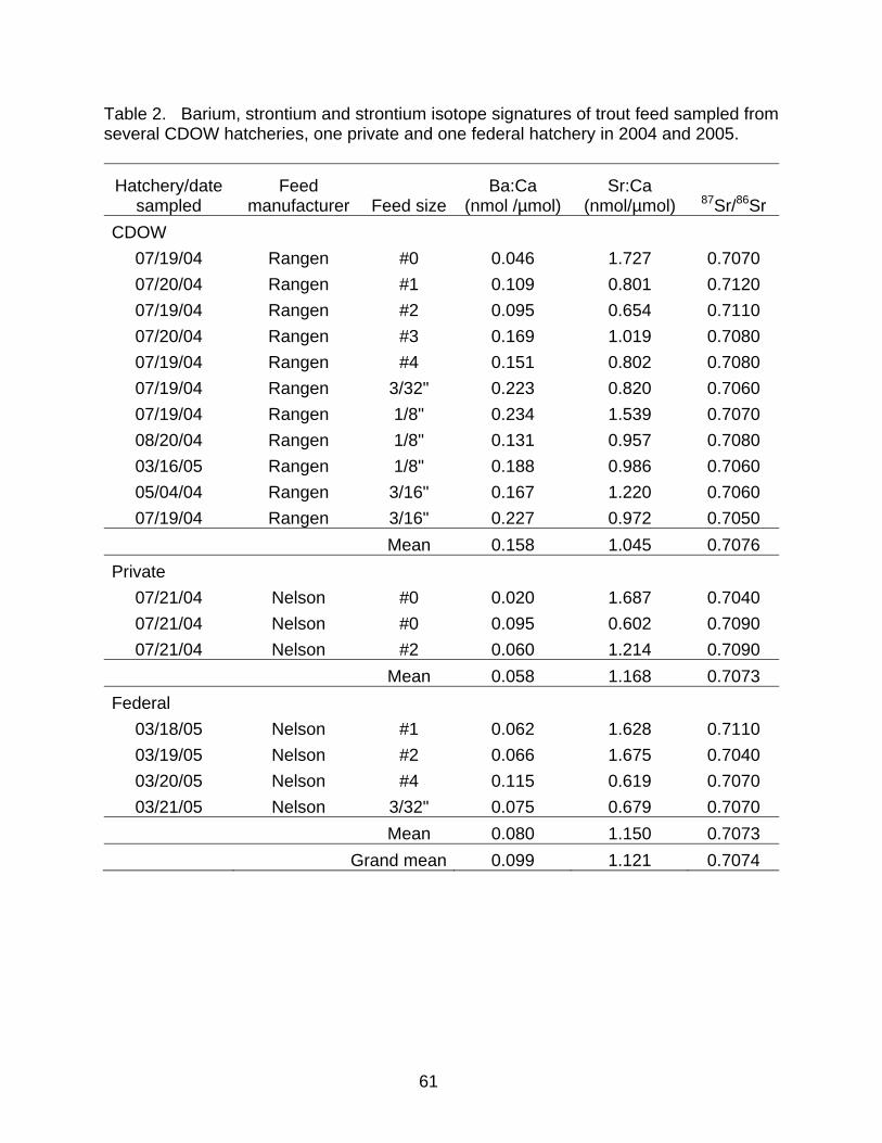
61
Table 2. Barium, strontium and strontium isotope signatures of trout feed sampled from several CDOW hatcheries, one private and one federal hatchery in 2004 and 2005.
Hatchery/date sampled
Feed manufacturer Feed size
Ba:Ca (nmol /µmol)
Sr:Ca (nmol/µmol) 87Sr/86Sr
CDOW 07/19/04 Rangen #0 0.046 1.727 0.7070 07/20/04 Rangen #1 0.109 0.801 0.7120 07/19/04 Rangen #2 0.095 0.654 0.7110 07/20/04 Rangen #3 0.169 1.019 0.7080 07/19/04 Rangen #4 0.151 0.802 0.7080 07/19/04 Rangen 3/32" 0.223 0.820 0.7060 07/19/04 Rangen 1/8" 0.234 1.539 0.7070 08/20/04 Rangen 1/8" 0.131 0.957 0.7080 03/16/05 Rangen 1/8" 0.188 0.986 0.7060 05/04/04 Rangen 3/16" 0.167 1.220 0.7060 07/19/04 Rangen 3/16" 0.227 0.972 0.7050
Mean 0.158 1.045 0.7076 Private
07/21/04 Nelson #0 0.020 1.687 0.7040 07/21/04 Nelson #0 0.095 0.602 0.7090 07/21/04 Nelson #2 0.060 1.214 0.7090
Mean 0.058 1.168 0.7073 Federal
03/18/05 Nelson #1 0.062 1.628 0.7110 03/19/05 Nelson #2 0.066 1.675 0.7040 03/20/05 Nelson #4 0.115 0.619 0.7070 03/21/05 Nelson 3/32" 0.075 0.679 0.7070
Mean 0.080 1.150 0.7073 Grand mean 0.099 1.121 0.7074

62
Table 3. Collection site, year, species, and total length of trout collected directly from hatcheries and used for chemical analyses of otoliths. Mean total length (TL, mm) is reported with standard deviation in parentheses. Dashes denote location/year combinations when no fish were collected.
2004 2005
Hatchery Date
sampled Mean TL n Date
sampled Mean TL n
BLV 09/03/04 116 (15)1 10 04/08/05 56 (4) 10
CCL 07/2104 294 (13) 10 03/15/05 251 (13) 10
CRU 07/19/04 311 (19) 10 03/17/05 03/17/05
288 (39) 70 (8)
10 10
DUR 07/20/04 276 (20) 10 03/14/05 244 (18) 10
GSU 07/19/04 221 (14) 10 03/17/05 121 (14) 10
MSH 07/21/04 139 (15)1 10 03/15/05 154 (19) 10
PRU 09/10/04 231 (27)1 10 04/08/05 230 (20) 10
RIF 07/20/04 283 (24) 10 03/17/05 230 (22) 10
ROJ 09/09/04 230 (27) 11 03/16/05 236 (34) 11
SLS 07/21/04 223 (12) 10 03/15/05 208 (17) 10
TFH -- -- -- 10/24/05 303 (24) 10
WAT 09/03/04 276 (23) 10 04/08/05 236 (16) 10 1rainbow x cutthroat hybrid

63
Table 4. Samples of fish that were known a priori to have resided at multiple hatcheries. We collected the fish from the destination hatchery at the specified size at collection on the date of collection shown (n = 10 in each case).
Hatchery of origin
Size when moved Date of transfer
Destination hatchery
Size at collection
(mm) Date
collected
BLV 5-6” March 2004 WAT 276 September
2004
BLV 5” August 2004 WAT 236 April 2005
BLV 5” August 2003 PRU 231 September
2004
BLV 7.5” August 2004 PRU 230 April 2005
MOH 3” November 2003 SLS 223 July 2004
MSH fingerlings unknown SLS 208 March 2005
TSP 2.5” June 2004 TFH 303 October
2005

64
Table 5. Hatchery of origin, site, date, and mean length (TL, mm) of at-large fish collected by CDOW researcher Kevin Thompson and provided to CSU as blind samples (“unknown origin fish”) for use in testing DFA classification models. Mean length is shown with SD in parentheses; mean length of fish collected in December was determined from fish grouped into size classes. Fish originating from DUR and RIF were known to be of the 2003 year class; other fish were of unknown age.
Hatchery of origin Collection site Date collected Mean TL n
ROJ ROJ channel 12/01/04 253 (--) 45
DUR ROJ ponds 11/12/04-11/30/04 301 (41) 27
RIF ROJ ponds 11/12/04-11/30/04 304 (23) 18
ROJ ROJ ponds 11/12/04 282 (19) 11
MSH/RIF Spring Creek 09/08/04 252 (18) 28

65
Table 6. Classification accuracy of 11 CDOW hatcheries using a discriminant function analysis with only Sr and Ba as classifiers. Accuracy is the percentage of otoliths from each location that were classified to the correct hatchery of origin by the discriminant function; n is the number of otoliths analyzed from each location. Bold numbers along the diagonal also indicate the percentage of otoliths from each hatchery that were correctly classified to their hatchery of origin. Some rows do not sum to exactly 100 due to rounding error. Average accuracy among locations was 59%.
Location Accuracy (percent) n
Location/accuracy (percent)
BLV CCL CRU DUR GSU MSH PRU RIF ROJ SLS WAT
BLV 70 17 70 0 10 0 0 0 0 0 0 0 20
CCL 76 17 0 76 18 0 0 0 0 6 0 0 0
CRU 39 28 0 21 39 7 0 0 0 11 0 0 21
DUR 84 19 0 0 0 84 0 5 0 5 0 5 0
GSU 67 18 5 0 0 0 67 0 5 0 4 0 0
MSH 58 19 0 0 0 11 0 58 0 0 0 32 0
PRU 40 20 10 5 5 0 0 0 40 0 25 0 15
RIF 72 18 0 0 17 11 0 0 0 72 0 0 0
ROJ 83 18 11 0 0 0 6 0 0 0 83 0 0
SLS 29 14 0 0 0 36 0 36 0 0 0 29 0
WAT 29 14 0 7 14 0 0 0 50 0 0 0 29

66
Table 7. Classification accuracy (percent) of DFA models for a blind sample of CDOW hatchery-reared fish captured at large after stocking. The 8 location model includes the four true sources as well as four hatcheries which were not sources of the fish, while the 4 location model uses only the four hatcheries from which the fish were stocked. The row “MSH/RIF” includes fish that were captured from locations that had been stocked by Mount Shavano and Rifle hatcheries. Otoliths from this group that were classified as MSH or RIF in a DFA model were classified as accurate, although we cannot provide further resolution for those samples.
Hatchery of origin n
8 location model accuracy
4 location model accuracy
ROJ 57 84 96
DUR 27 64 73
RIF 18 53 73
MSH/RIF 28 36 68
Average accuracy 59 79

67
Table 8. Percentage of otoliths classified to each of 5 hatcheries in a DFA model using Sr:Ca, Ba:Ca, and 87Sr/86Sr and a DFA with only Sr:Ca and Ba:Ca (in parentheses). Average accuracy was 96% for the model including 87Sr/86Sr and 63% for the model without 87Sr/86Sr.
Hatchery n CCL CRU MSH PRU SLS
CCL 5 100 (60) 0 (40) 0 (0) 0 (0) 0 (0)
CRU 5 0 (60) 80 (20) 20 (0) 0 (0) 0 (20)
MSH 4 0 (0) 0 (0) 100 (75) 0 (0) 0 (25)
PRU 3 0 (0) 0 (0) 0 (0) 100 (100) 0 (0)
SLS 5 0 (0) 0 (0) 0 (40) 0 (0) 100 (60)

68
Table 9. Fish originating in public hatcheries and moved to a different location and the ability of otolith chemistry to detect such movements. Strontium abundance was analyzed for fish from all hatcheries, but fish from only three hatcheries were analyzed for 87Sr/86Sr (n = number of otoliths analyzed for each marker, SD in parentheses). The first row (BLV to BRR) represents fish collected in Button Rock Reservoir, CO, and the last row shows fish collected from Tillet Fish Hatchery (TFH) in Wyoming (see Table 4).
Hatchery of origin
Collection site (year)
Mean Sr (ppm) Mean 87Sr/86Sr
n Core Edge n Core Edge
BLV BRR (2006) 19 Change between core and edge in 11 of 19 5 0.7112
(0.0004) 0.7345
(0.0006 )
BLV PRU (2004) 10 No changes detected 0 Not analyzed
BLV PRU (2005) 10 No changes detected 3 0.7112 (0.0002 )
0.7170 (0.0027 )
BLV WAT (2004) 4 No changes detected 0 Not analyzed
BLV WAT (2005) 10 No changes detected 0 Not analyzed
MOH SLS (2004) 4 No changes detected 0 Not analyzed
MSH SLS (2005) 10 No changes detected 5 0.7105 (0.0011 )
0.7085 (0.0005 )
TSP TFH (2005) 10 412 (95) 860 (41) 0 Not analyzed

69
DUR
FRO
GSURIF
CRU
SLS
ROJPKN
PRUFRH
CCL
MOHMSH
MVU
BLVWAT
Figure 1. Geologic map of Colorado showing approximate locations of 16 CDOW trout hatcheries sampled during 2004-2006. The 11 hatcheries that were used for developing the DFA models are shown in green.

70
Figure 2. Polished thin section of an otolith extracted from a rainbow trout collected from the Crystal River Hatchery on March 17, 2005, viewed under transmitted light (upper panel) and reflected light (lower panel). A furrow ablated by the LA-ICP-MS laser can be seen running longitudinally from the left side of the otolith to a point about 250 µm to the right of the otolith’s core.

71
0.000
0.200
0.400
0.600
0.800
1.000
1.200
1.400
1.600
1.800
Hatchery
Sr:C
a(m
mol
:mol
)
(4)
(4)
(8)(9)
(9)
(9)
(8)(8) (18)
(9)
0.000
0.001
0.002
0.003
0.004
0.005
0.006
0.007
0.008
0.009
0.010
Ba:
Ca
(mm
ol:m
ol)
(4)
(4)
(8)(9)
(9)
(9)(8)(8)
(18) (9) (9)
CCL CRU DUR GSU MSH PRU RIF ROJ SLS WATCCL CRU DUR GSU MSH PRU RIF ROJ SLS WAT
CCL CRU DUR GSU MSH PRU RIF ROJ SLS WATCCL CRU DUR GSU MSH PRU RIF ROJ SLS WAT
Figure 3. Mean Barium (Ba) and strontium (Sr) concentrations (± SD) in otolith samples from 10 CDOW trout hatcheries sampled in 2004 (□) and 2005 (■). Data from BLV were not used because of physical and chemical abnormalities in otoliths collected in 2005. Sample size was 10 fish unless shown.

72
0.0
0.2
0.4
0.6
0.8
1.0
1.2
BLV
CC
L
CR
Us
CR
Uw
DU
R
FRH
FRO
GSU
c
GSU
s
MO
H
MSH
MVU PI
K
PRU
RIF
RO
Js
RO
Jw
SLS
WAT
Ba:
Ca
(mm
ol:m
ol)
200420052006
0.01.02.03.04.05.06.07.08.0
BLV
CC
L
CR
Us
CR
Uw
DU
R
FRH
FRO
GSU
c
GSU
s
MO
H
MSH
MVU PI
K
PRU
RIF
RO
Js
RO
Jw SLS
WAT
Sr:C
a (m
mol
:mol
) 200420052006
Figure 4. Strontium (Sr) and barium (Ba) concentrations (normalized to calcium) in water samples collected at 16 CDOW trout hatcheries during 2004, 2005, and 2006. Multiple water sources were sampled at CRU, GSU, and ROJ; subscripts “s”, “w”, and “c” denote spring, well, and creek samples, respectively. All other hatcheries had only one water supply type. Replicate samples were only collected in 2006; bars represent the mean of three to six samples per location collected on a single day, plus or minus one standard deviation. No data were available for some site/years.

73
0.7000
0.7040
0.7080
0.7120
0.7160
0.7200
0.7240
BLV
CC
L CR
U
DU
R
GSU
MSH
PRU
RIF
RO
J
SLS
WA
T
200420052006
87Sr
/86Sr
Figure 5. Strontium isotope ratio of water samples collected from 11 CDOW hatcheries plotted as difference from the global freshwater mean (0.711; Graustein 1988). Replicate samples were only collected in 2006; bars represent the mean of three to six samples per location collected on a single day, plus or minus one standard deviation.

74
0.0
0.4
0.8
1.2
1.6
0.0 2.0 4.0 6.0 8.0 10.0Water Sr:Ca (mmol:mol)
Oto
lith
Sr:C
a (m
mol
:mol
) 20042005
0.0
2.0
4.0
6.0
8.0
10.0
0.0 0.2 0.4 0.6 0.8 1.0 1.2 1.4Water Ba:Ca (mmol:mol)
Oto
lith
Ba:
Ca
(nm
ol:m
ol) 2004
2005
Figure 6. Mean barium (Ba) and strontium (Sr) concentrations (± SD) in otoliths and in water samples at 11 CDOW trout hatcheries sampled in 2004 and 2005.

75
0%
25%
50%
75%
100%
024681012Number of locations
Cla
ssifi
catio
n ac
cura
cy DFA model
chance alone
Figure 7. Results of Monte Carlo simulation showing effect of group size on classification accuracy when sets of 10 to 2 hatcheries were randomly selected from the pool of 11 study hatcheries. Circles represent the average accuracy (plus or minus 1 SD) of models based on 10 analyses per group size (all 11 combinations of 10 hatcheries were used for the group size of 10). The solid line represents the expected accuracy of models due to chance alone.

76
y = 0.480x + 0.369r2 = 0.84n = 35
0.7000
0.7040
0.7080
0.7120
0.7160
0.7200
0.7240
0.700 0.704 0.708 0.712 0.716 0.720 0.72487Sr/86Sr (water)
87S
r/86S
r (ot
olith
)1:1
Marine
Figure 8. Strontium isotope ratios in hatchery reared trout as a function of the isotope ratio in the water at each hatchery. The 1:1 line represents the slope that would be expected in wild fish (Kennedy et al. 2002; Ingram and Weber 1999). The solid black line represents the slope of the relationship between otolith and water chemistry in our samples, indicating a strong “pull” of marine derived hatchery feed. The Marine bar indicates the global seawater value of 87Sr/86Sr.

77
-150
-140
-130
-120
-110
-100
-90
-80
BLV
CC
L
CR
U
DU
R
FRH
FRO
GSU
GSU MO
MSH
MVU
MVU PI
K
PRU
RIF
SLS
WAT
δ D (‰
)
Hatchery
Groundwater Surface water
Figure 9. Deuterium signature (δD) of water samples taken from 15 trout hatcheries during July 2004. Three facilities had exclusively surface water supplies (CCL, PRU, WAT), all others were supplied by groundwater sources or a mix of surface and groundwater. Dashed lines show the maximum and minimum δD reported for Colorado surface waters in Coplen and Kendall (2000). Two measurements at MVU represent samples from a shallow (18 m) well and a deep (760 m) well.

78
Scenario B
HatcheryA
HatcheryB
Collectionsite
Scenario C
HatcheryA
HatcheryB
Collectionsite
Scenario C
HatcheryA
HatcheryB
Collectionsite
HatcheryA
HatcheryB
Collectionsite
Scenario D
HatcheryA
HatcheryB
Collectionsite
Scenario A
HatcheryA
HatcheryB
Collectionsite
Figure 10. Four hypothetical stocking scenarios and how they are perceived by examination of otoliths of the stocked fish. In each panel, arrows represent direction of fish movement (solid lines = perceived, dashed lines = actual), Hatchery A is where the fish were hatched and reared to some size before being stocked at their final destination (Scenario A) or being moved to Hatchery B (Scenario B, C, D) and subsequently being stocked at their final destination. Cross-hatching represents water chemistry; in Scenarios A and B water chemistry differs among the three locations, but there are only two unique chemistries in Scenarios C and D. In Scenario C, water chemistry of Hatchery A differs from that of Hatchery B and the Collection site, which share the same water chemistry; thus, fish transferred from Hatchery A to B before being stocked at the final destination appear to have been stocked directly from Hatchery A, based on otolith chemistry. This outcome could also arise if fish are moved from Hatchery A to Hatchery B for a short time before being stocked at the Collection site, regardless of the distinctiveness of Hatchery B’s water chemistry. In Scenario D, fish may be moved between hatcheries with similar water or not prior to stocking, neither movement nor the exact source are discernible from otolith chemistry.

79
Likelysource
IsotopicmarkersIsotopicmarkers
Elementalmarkers
Elementalmarkers
“Stock”characteristics
“Stock”characteristics
Classical detective work
Classical detective work
Potentialsources
Strain, molecular genetics, morpho-meristics
Stocking records, eye witness accounts, personal interviews
Examples
Strontium, barium in otoliths
87Sr/86Sr, 2H/1H in otoliths
Outcome may be a match to a suspected source or a detailed description of source hatchery’s chemistry and local geology
Figure 11. In the “Eclectic Approach to Source Identification” multiple lines of evidence are used to narrow the pool of suspects until the most likely source of an illegal introduction is identified, or until a detailed chemical signature of the source hatchery and its surrounding geology can be constructed from the illegal fish’s otoliths. With this approach investigators glean new information from otolith chemistry unattainable by conventional methods while their conventional methods serve to narrow the pool of suspects, thereby enhancing the effectiveness of classification models developed from otolith chemistry.

80
Appendices
Appendix 1. Non-technical project summary
Appendix 2. Photos related to the project.
Appendix 3. Procedures
Appendix 4. Cost and labor estimates

81
Appendix 1. Non-Technical Project Summary One of the continued threats to viable trout populations in the Mountain West is
the spread of whirling disease via illegal stocking of diseased trout. Attempts to halt
such introductions and prosecute violators have been twarted because it has been
virtually impossible to trace the origins of a diseased trout once it has been stocked.
Naturally occurring chemical markers in fish tissue have shown promise as a method to
track the origins of fish in previous studies. However, research to date had not looked
at the potential for these markers to work adequately in hatchery environments over
large areas or to distinguish many potential source hatcheries. We evaluated the use of
chemical markers in fish otoliths, or “ear stones,” to determine the hatchery of origin of
stocked trout.
We found that otolith markers could be highly effective markers of the past
environmental history of trout. We sampled 11 hatcheries and several populations of
stocked trout captured from public waters, simulating conditions that may occur in a
forensic case. Our ability to correctly identify the hatchery the fish came from increased
with the number of chemical markers used (and hence cost) and when there were fewer
“suspect” hatcheries. Otoliths are capable of providing information about the location a
fish has inhabited, a feat not achievable with any other technique. The information from
otoliths is best used to fill gaps in cases where traditional methods of investigation have
been adequately conducted. The result of this research will provide law enforcement
with a valuable tool to prosecute those who have illegally stocked trout and serve as a
deterrent to future illegal stockings. Thus, we have provided a useful tool to help
preserve the biological and economic health of trout fisheries.
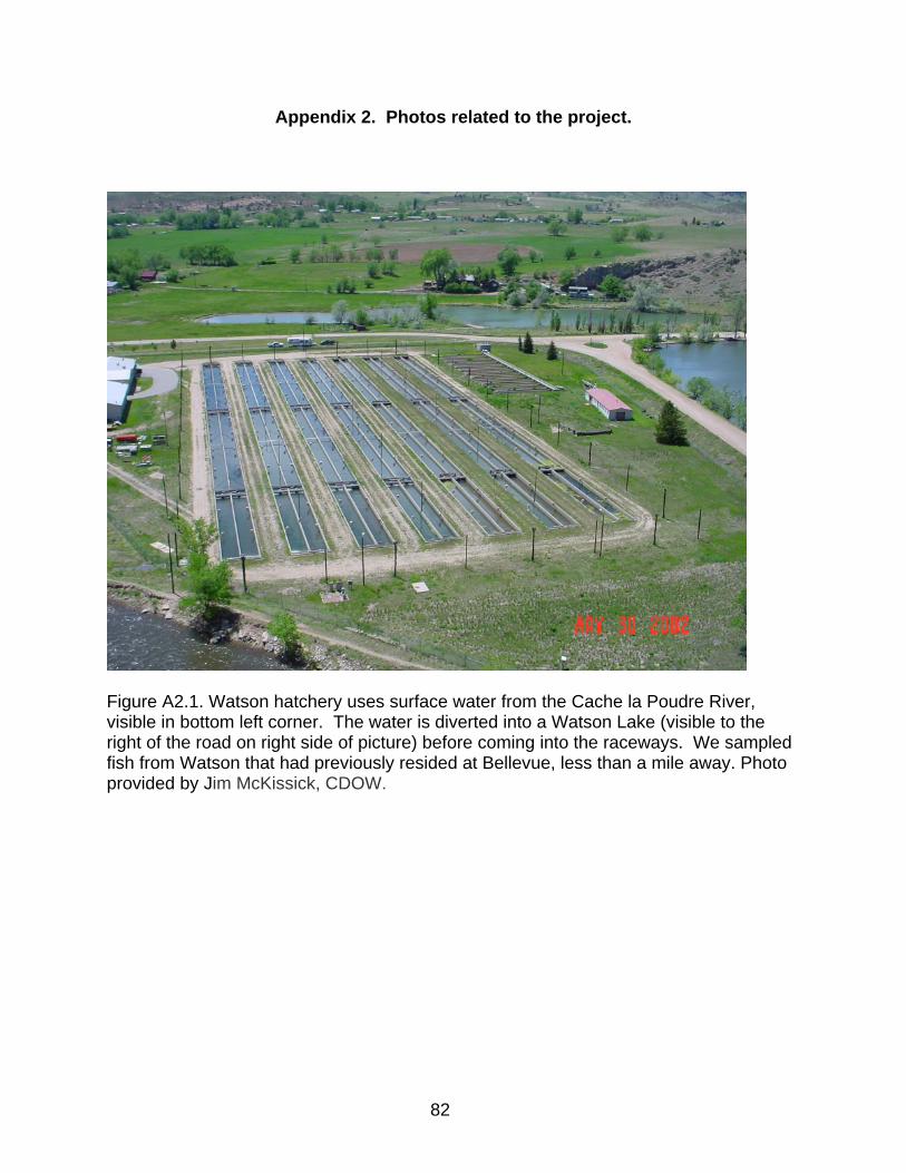
82
Appendix 2. Photos related to the project.
Figure A2.1. Watson hatchery uses surface water from the Cache la Poudre River, visible in bottom left corner. The water is diverted into a Watson Lake (visible to the right of the road on right side of picture) before coming into the raceways. We sampled fish from Watson that had previously resided at Bellevue, less than a mile away. Photo provided by Jim McKissick, CDOW.
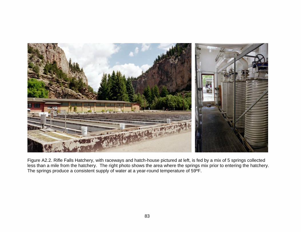
83
Figure A2.2. Rifle Falls Hatchery, with raceways and hatch-house pictured at left, is fed by a mix of 5 springs collected less than a mile from the hatchery. The right photo shows the area where the springs mix prior to entering the hatchery. The springs produce a consistent supply of water at a year-round temperature of 59ºF.

84
Figure A2.3. Water was collected using clean techniques. In some instances, hatcheries used multiple water sources and samples were collected after they had been thoroughly mixed prior to entering raceways, as shown above.

85
Figure A2.4. Configuration of the trout culture facilities sampled in this study varied greatly from place to place. Above: Finger Rock hatchery, right: Mount Shavano hatchery (photo: Jim McKissick, CDOW).

86
Appendix 3. Procedures
Table A3.1. Abridged (not complete!) procedures for the collection of samples for determination of origin and movement of illegally stocked fishes. We recommend that both otoliths and tissue samples be taken from fish; this allows for both microchemical analysis and molecular genetic analysis. It is essential that tissue and otolith samples be given the same identifier so data from each can be matched up later.
______________________________________________________________________
Otoliths
We assume that otoliths will be subjected to microchemical analysis by LA-ICP-MS. Note that risk of contamination is much greater for solution-based approaches, as opposed to the laser transect methods we used. See Campana (2000) for additional precautions necessary for handling otoliths prior to solution-based analysis.
1. The number of fish to collect can be determined from a power analysis or based on the present study’s guideline: 13 fish per location.
2. Handling otoliths with nonmetallic forceps is not critical but is recommended.
3. Record detailed collection information (date, collection site, length, weight, species/strain, etc.)
4. Remove saggital otoliths from fish immediately after capture (or freeze fish until otoliths can be removed). Do not store fish or otoliths in liquid preservative.
5. Remove all tissue adhering to otoliths and rinse with deionized distilled water.
6. Place otolith pair in labeled polyethylene microcentrifuge tube, and store tube in labeled coin envelope.
7. Store coin envelopes in sealed Whirlpak or Ziploc bag until otoliths can be embedded, sectioned, and polished or sent to analytical laboratory.
Tissue samples
We recommend following the protocol for collecting trout tissues for genetic analysis developed in 2007 by Kevin Rogers, Aquatic Wildlife Research Biologist, CDOW ([email protected]). In a nutshell, this protocol states:
1. Use scissors to remove at least a 1-cm2 piece of the top of the caudal fin.
2. Store tissue in 15 mL polypropylene, “plug-seal” centrifuge tube with denatured reagent grade ethanol diluted to 80% with distilled water.
3. Do not place anything (e.g., a label) inside the centrifuge tube with the tissue/ethanol or it might compromise the DNA analysis. Rather, write on the outside of the tube with a special purpose laboratory marker.
______________________________________________________________________

87
Table A3.1. Abridged procedures- continued.
______________________________________________________________________
Water
We followed the procedure of Shiller (2003; [email protected]) to collect clean water samples for trace element and isotope analysis. This protocol is best accomplished with two people, a “clean hands” person and a “dirty hands” person. Great care must be taken to avoid sample contamination. The procedure consists of two parts:
1. Samples collection. We used Method B. Immerse a pre-cleaned 250 or 500 mL bottle in the water source, rinse a couple times, then immerse and invert under water and cap it.
2. Sample filtration. This is quite tedious and time-consuming, and this is usually the stage with the most serious potential for sample contamination.
a. Given the windy and dusty conditions typical of the mountain west, we strongly recommend filtration be done indoors, if possible. However, filtration should also be done soon after samples are collected. When away from buildings, we did our filtration inside a tent or inside the topper of a pickup truck.
b. There are several steps to this protocol, resulting in 2 replicate 15 mL samples of filtered water. You will double bag the plastic sample bottles in ziplocks, and keep them cool and in the dark until you can ship them to Dr. Shiller’s lab for trace chemistry analysis.
______________________________________________________________________

88
Appendix 4. Cost and labor estimates
Table A4.1. Required supplies, sources, and approximate costs ($US, 2006; laboratories may charge higher rates for commercial or private clients) for sample collection, preparation and analysis associated with the use of otolith microchemistry for forensic applications. Asterisked items are not essential but very useful.
Sample Collection Supplies/equipment Source Cost Otoliths per unit
Coin envelopes (2-1/2'' X 3-1/2'') Office supply outlets $20 per
500 One pair
Gloves, other field supplies various $100 $100 per additional 100 samples
Microcentrifuge tubes (1.5 mL)
Scientific supply outlets
$20 per 500 One pair
Non metallic forceps Scientific supply outlets
$10 per each Thousands
Ultra-clean collection water kits
Center for Trace Analysis, Univ. of
Southern Mississippi
$25 per each N/A
Otolith Preparation Supplies/equipment Source Cost Otoliths per unit
Isomet Low Speed Saw Buehler Ltd. $4,500 Thousands
Saw blades (Norton) Grainger Industrial Supply $300 >75
Other saw supplies (dressing sticks, cutting fluid) Buehler Ltd. $50 Dozens
Epoxy mounting kit Electron Microscopy Sciences $150 >200
Sandpaper, slides, miscellaneous supplies Hardware stores $150 $100 per additional
100 otoliths Stereomicroscope, camera*,
image analysis software* Scientific supply
outlets $10,000 Unlimited
Lapidary polishing machine* Ameritool Inc. $329 Thousands
Chemical Analysis Sample:analytes Cost per sample Laboratory used in this study Water:elements
and 87Sr/86Sr $85, minimum
$350 Center for Trace Analysis, University of
Southern Mississippi
Water:2H $27 Water and Environmental Research Center, University of Alaska-Fairbanks
Otolith: elements $10; $1,200/day USGS Mineral Resources Laboratory, Lakewood, CO
Otolith: 87Sr/86Sr $65; minimum $1,270
Isotope & Trace Element Geochemistry Group, University of Melbourne, Australia
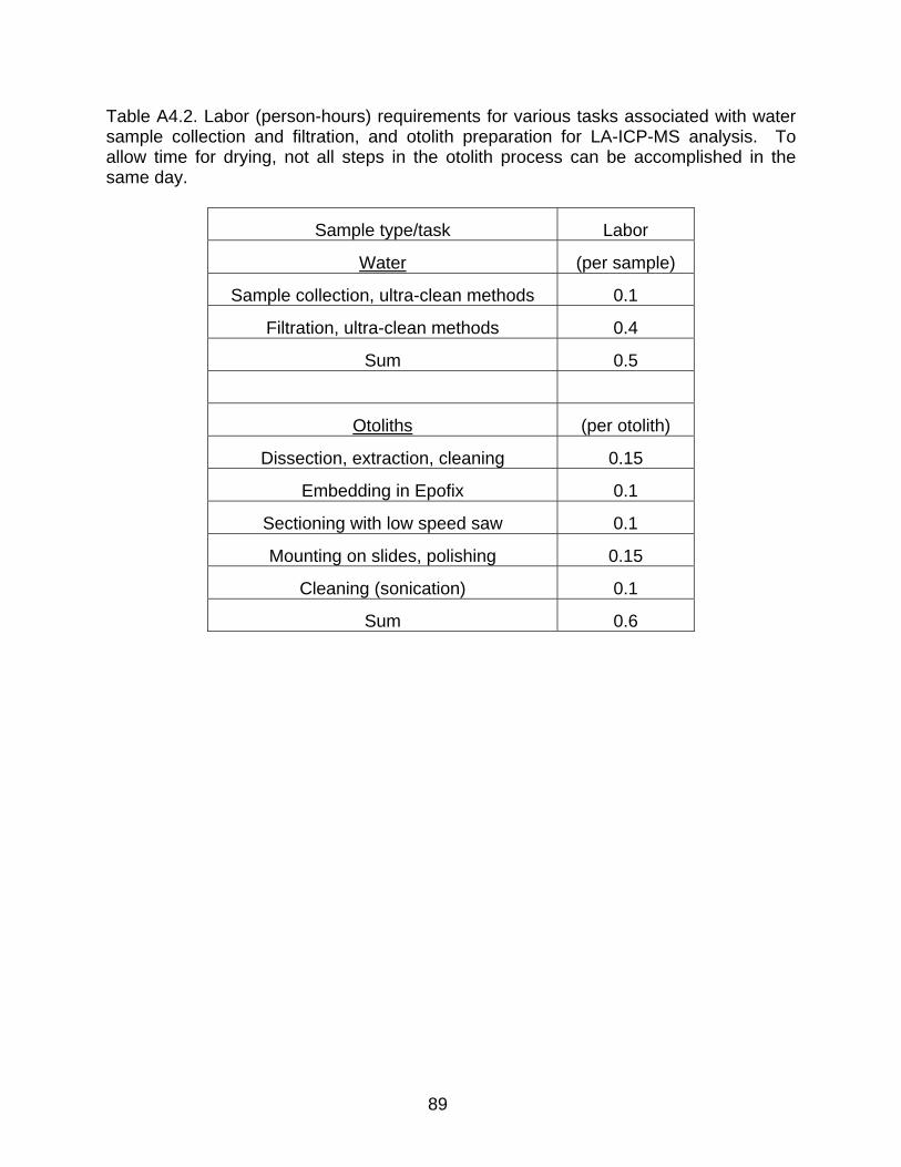
89
Table A4.2. Labor (person-hours) requirements for various tasks associated with water sample collection and filtration, and otolith preparation for LA-ICP-MS analysis. To allow time for drying, not all steps in the otolith process can be accomplished in the same day.
Sample type/task Labor
Water (per sample)
Sample collection, ultra-clean methods 0.1
Filtration, ultra-clean methods 0.4
Sum 0.5
Otoliths (per otolith)
Dissection, extraction, cleaning 0.15
Embedding in Epofix 0.1
Sectioning with low speed saw 0.1
Mounting on slides, polishing 0.15
Cleaning (sonication) 0.1
Sum 0.6

90
APPENDIX C
POWERPOINT PRESENTATION:
CONCEPTS, CONCERNS & CONFLICTS IN THE MANAGEMENT OF NATIVE FISH SPECIES & NONNATIVE
SPORT FISHES IN THE WESTERN UNITED STATES

Concepts, Concerns & Conflicts in the Management of Native Fish
Species & Nonnative Sport Fishes in the Western United States
Patrick J. MartinezAquatic Researcher
Colorado Division of Wildlife
Grand Junction
November 2007
- contrast sport fish recreation & native fish conservation
Key concepts & issues:
- challenges & concepts in native sport fish conservation
- professionalism, advocacy & activism
- magnitude of nonnative fish abundance in western US
- issues & obstacles in nongame native fish conservation
- conflict between sport fish & native fish management
- growing plight of SW nongame native fish populations
- urgency for nongame native fish conservation areas
- illicit stocking highly detrimental to sport & native fish
91

N. American Wildlife Conservation Model
Nongame Aquatic Wildlife
Endangered Species Act (ESA) – key sections
1. Public trust2. No commerce3. Democratic rule4. Equal opportunity5. Non-frivolous use6. International resources7. Scientific mgmt.
-Prey, bait-Commercial-Food webs & evolutionary proc.
-Often must become imperiled to receive cons. effort & resources
4. Species listing4. Critical habitat4. Recovery plans6. Cooperation with states7. Interagency consultation8. International cooperation9. Enforcement
Harvestable surplus, naturally or artificially sustained
Harvestable or expendable surplus
Last chance, remnant numbers, genetic concerns, reproductive potential
Sportsman license fees & equipment surcharges Lottery & check-off Taxes & depletion fees
Fishing quality & diversity Species inventory Biodiversity & ecosystem
integrity
Economic clout Ecological function Environmental clout
Biodiversity: large variety of native species sustained by a variety of quality habitats suitable for these species
92

Quist & Hubert. 2004. Bioinvasive species & preservation of cutthroat trout in the western US: ecological, social & economic issues. Enviro. Science & Policy 7:303-313.
-most T&E fish listed under ESA occur in western US
Cutthroat trout:-had broadest distribution of any trout species in NA
-14 recognized subspecies (Behnke 2002)
-many factors in cutthroat decline; most significant nonnative fish species
-greatest negative impact has been introduced nonnative trout
-nearly all reduced to <5% of their historic distributions
-2-extinct, 2-federally listed, several petitioned for ESA, most state listed
-four nonnative trout = greatest influence: rainbow, brook, brown & lake
-widespread nonnative salmonids is legacy of past management practices
Quist & Hubert. 2004.
Nonnative trout Species
Rainbow competition & hybridization - all habitats
Brook competition & reproduction -small streams
Brown comp.,repro.& predation -large streams
Lakepredation –large lakes
Conceptual model of risks associated with preservation of cutthroat trout
93

Quist & Hubert. 2004.
Nonnative trout Species Ecosystem
Rainbow competition & hybridization - all habitats
similar ecology, little or no effect
Brook competition & reproduction -small streams
ecological equivalent in
streams
Brown comp.,repro.& predation-
large streams
also prey on other native fish species
Lakepredation –large lakes
impacts also extend to terrestrial
Conceptual model of risks associated with preservation of cutthroat trout (con’t)
Quist & Hubert. 2004.Social issues associated with preservation of cutthroat trout
- value of native fish protection has increased among resource professionals
- view & value of protecting native fish differs among public
- Ethical: spp. have intrinsic value, deserve protection, indicate environmental heath & ecological integrity should be preserved for future generations Public may oppose killing nonnative trout to protect cutthroat trout
- Aesthetic: assoc. with viewing natural beauty of spp. & their habitat Public & anglers may not differentiate between native vs. cutthroat trout
- Historical: spp. role in history of particular water, region, culture or individual & historic value in subsistence, commercial & recreational fisheries Public & anglers now associate nonnative trout with cutthroat habitats
- Recreational: little effect from replacement of cutthroat by nonnative trout Anglers often have no preference or strongly prefer nonnative trout Anglers fear loss of angling opportunity due to cutthroat protections
- nonnative trout viewed most detrimental in areas valued as pristine
94

Quist & Hubert. 2004.
Nonnative trout Species Ecosystem Economics
Rainbow competition & hybridization - all habitats
similar ecology, little or no effect
Little social or economic
justification to control nonnative trout. Cutthroat
preservation can be costly with
little or no economic
benefit. Control warranted by
evolutionary & ecological
values. Must convince public.
Brook competition & reproduction -small streams
ecological equivalent in
streams
Brown comp.,repro.& predation-
large streams
also prey on other native fish species
Lakepredation –large lakes
impacts also extend to terrestrial
Conceptual model of risks associated with preservation of cutthroat trout (con’t)
Cate-gory
F-1
F-2
F-3
Scale for Engaging Fishery Management Scenarios: Resource Risk, Professional Angst & Activism?
Habitat status
Artificial or altered
Artificial to pristine
Altered or pristine
Species involved
Traditional & established nonnative sport fish
Traditional, established, & proposed nonnative sport fish
Traditional, established, & proposed nonnative sport fish & native fishes
Impact footprintLocal, e.g tailwater or reservoir
Multiple stream-miles or reservoirs
Local, drainage-or basin-wide
Ethics, ecology, & economics ($$)
Provide professional expertise; fishery preference & quality; stocking & special regulations; local $$Invoke ethics; multi-spp.interactions; fishery stability & compatibility; food webs, predator-prey & broodstocks; local to regional $$Reveal values; public trust; dual-mission; fishing diversity vs. bio-diversity; recreation vs. preservation; local to national $$; activism?
Advocates & “Referees”
Anglers, businesses, fishery agency
Multiple resource agencies, conservationists
Multiple regulatory agencies, conservationists, general public
95

Schade & Bonar. 2005. Distribution & abundance of nonnative fishes in streams of the western US. NAJFM 25:1386-1394.
-nonnative fish contribute to decline in biodiversity of US streams through predation, competition and hybridization
-% of stream length with nonnative fish: CO=73%; MT=69%; AZ=67%, UT=66%; ND=61%
-12 western states,1 in 4 fish nonnative; CO, 2 in 3 fish nonnative; AZ, 1 in 2 fish nonnative: ND, 1 in 12 fish nonnative
->50% of fish spp. nonnative in AZ=59%, CO=53%, ND=52%
-stream length with spp. present: BKT=17%; BNT=15%; RBT=11%, CCP=9%; SMB=6%; LMB=3%
-abundance of nonnative vs. native fish inversely related
-interior west states have low native species diversity & higher endemism; SW has highest number of extinct fish species
Schade & Bonar. 2005.-majority of most prominent nonnative fishes continue to be stocked for angling
-preservation of native fish must consider implications of stocking nonnative sport fish & need to eliminate of mitigate their impact
-nonnative fish abundant in both disturbed & undisturbed streams; WW species more prevalent in less pristine streams
-habitat destruction & nonnative fish can lead to population fragmentation & local or regional extinction of native fishes
-native fish displayed consistent negative association with presence, abundance & density of nonnative fish
-nonnative fish present in greater proportion of streams (50%) than affected by moderate to high level of human impact (18%)
-nonnative fish pose equal, if not greater, threat to native fishes than habitat degradation in western US streams
96
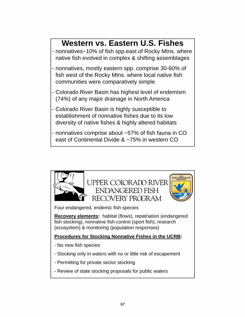
- Colorado River Basin has highest level of endemism (74%) of any major drainage in North America
- nonnatives, mostly eastern spp. comprise 30-60% of fish west of the Rocky Mtns. where local native fish communities were comparatively simple
- nonnatives~10% of fish spp.east of Rocky Mtns. where native fish evolved in complex & shifting assemblages
Western vs. Eastern U.S. Fishes
- Colorado River Basin is highly susceptible to establishment of nonnative fishes due to its low diversity of native fishes & highly altered habitats
- nonnatives comprise about ~57% of fish fauna in CO east of Continental Divide & ~75% in western CO
Four endangered, endemic fish species
Recovery elements: habitat (flows), repatriation (endangered fish stocking), nonnative fish control (sport fish), research (ecosystem) & monitoring (population responses)
Procedures for Stocking Nonnative Fishes in the UCRB:
- No new fish species
- Stocking only in waters with no or little risk of escapement
- Permitting for private sector stocking
- Review of state stocking proposals for public waters
97
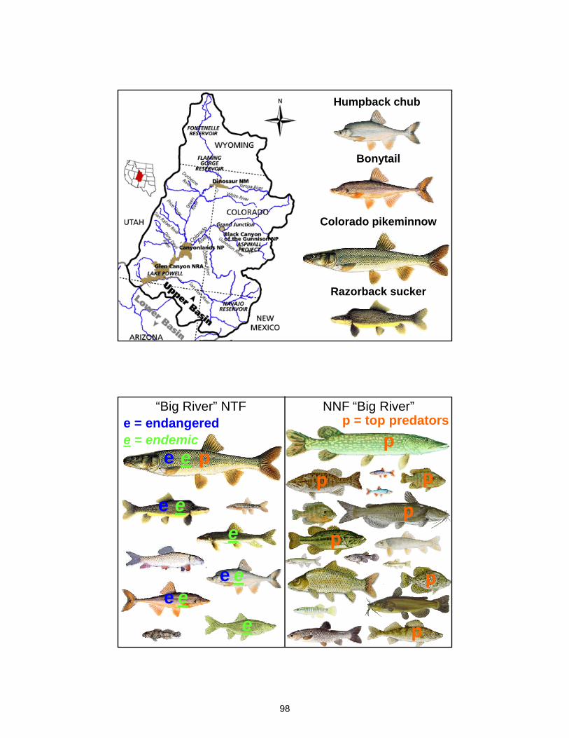
Bonytail
Colorado pikeminnow
Razorback sucker
Humpback chub
“Big River” NTF NNF “Big River” e = endangered
e
e
ee
e = endemice
ee
ee
e
p = top predators
pp
p
p
p
p
p
p
98

Clarkson et al. 2005. Conflicts between native fish & nonnative sport fish management in the SW US. Fisheries 30:20-27.
-early declines of SW native fishes:habitat destruction & alteration
-nonnative fish preclude or negate habitat protection or restoration
-greatest factor preventing preservation/recovery of SW native fish
-habitat restoration must include elimination of nonnative fishes
-nonnative fish mostly piscivores; natives mostly generalists
-native fish predator-naive; nonnatives co-evolved with predators
-nonnatives phylogenetically advanced; sophisticated life history
-natives broadcast spawners; no parental care of young
-differences in life histories results in failure of native to recruit
Clarkson et al. 2005.
-state & federal F&W agencies have dual missions/management responsibilities for native (T&E) & nonnative sport fish
-1996 “Conserving Spp. Listed or Proposed for Listing under ESA” acknowledged conflict in T&E recovery & nonnative sport fish
-sought to resolve conflict through increased public education & involvement in native fish recovery programs; agencies & anglers
-did not stop nonnative fish stocking in waters with T&E or proposed native fish; evaluation of ecological/economic impacts
-policy has generally been ignored by mgmt. agencies in SW
-little USFWS funding for nongame fishes, T&E authority & funding diluted by MOAs which increase state’s role in recovery
-should foster recovery, but states lack authority to implement ESA, no citizen legal redress, thus MOAs weaken recovery
99

Clarkson et al. 2005.-native fishes continue to decline & recovery actions undertaken or proposed for T&E fish ineffective, neglected or avoided
-conflict exists between nonnative sport & native nongame fish management & interests; conflicts resolved in favor of sport fish
-native trout mgmt.: nonnative fish removal, barriers to prevent recontamination – should be used for nongame native fishes
Solutions:
-designate small & medium WW streams solely for native fishes
-interconnectedness impt. for genetics & population fragmentation
-institutional change to autonomy for native nongame fish staff
-control transfers of undesirable spp.; prop. to angling activity
-strong policy statement supporting native nongame fishes
-dedicated funding for native nongame fish conservation
PUBLISHED ON FEBRUARY 1, 2007 in Tuscon Weekly: Fish Tale - Scientists smell something fishy behind dropping native populations By Tim Vanderpool
-biologists took the government to task for failing to protect AZ’ endangered fishes
-AG&FD is neglecting its native fish, while toadying up to sport-fishing
-sport-fishing pumps nearly $14 million annually into agency coffers
-recovery plans for endangered species aren't being carried out by state wildlife officials
-aggressive imports, LMB, BBH & SNF are wreaking havoc on native species
-"The recovery plans are sound but there is not consistent follow-through.“
-conflicting USFWS mandate protects native fish vs. state promotion of sport fishing
-"totally not true“: AZ favors lucrative sports fish over unglamorous, endangered natives”
-nonnative impact overplayed; other issues: dams, water diversion & habitat destruction
-must address this before removing nonnative sport fish & converting to native fish
100
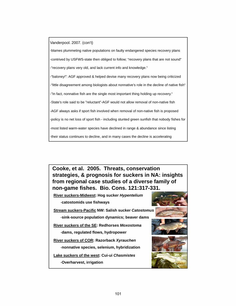
Vanderpool. 2007. (con’t)
-blames plummeting native populations on faulty endangered species recovery plans
-contrived by USFWS-state then obliged to follow; “recovery plans that are not sound“
-“recovery plans very old, and lack current info and knowledge.“
-“baloney!”: AGF approved & helped devise many recovery plans now being criticized
-“little disagreement among biologists about nonnative’s role in the decline of native fish“
-"In fact, nonnative fish are the single most important thing holding up recovery.“
-State's role said to be "reluctant”-AGF would not allow removal of non-native fish
-AGF always asks if sport fish involved when removal of non-native fish is proposed
-policy is no net loss of sport fish - including stunted green sunfish that nobody fishes for
-most listed warm-water species have declined in range & abundance since listing
-their status continues to decline, and in many cases the decline is accelerating
Cooke, et al. 2005. Threats, conservation strategies, & prognosis for suckers in NA: insights from regional case studies of a diverse family of non-game fishes. Bio. Cons. 121:317-331.River suckers-Midwest: Hog sucker Hypentelium
-catostomids use fishways
Stream suckers-Pacific NW: Salish sucker Catostomus
-sink-source population dynamics; beaver dams
River suckers of the SE: Redhorses Moxostoma
-dams, regulated flows, hydropower
River suckers of COR: Razorback Xyrauchen
-nonnative species, selenium, hybridization
Lake suckers of the west: Cui-ui Chasmistes
-Overharvest, irrigation
101

Northern Hog Sucker (Hypentelium nigricans)Unlike the majority of other species of suckers in Ohio which are primarily pool oriented, the hog sucker is adapted for life in fast currents and is found in riffles, chutes, and runs of the larger and medium-sized streams throughout the state.
Hog suckers require substrates composed primarily of clean gravels and cobbles where they feed on the aquatic insect larva which live in these substrates.
They are adversely impacted by siltation of instream habitats which destroys their food base and limits their reproductive success.
102
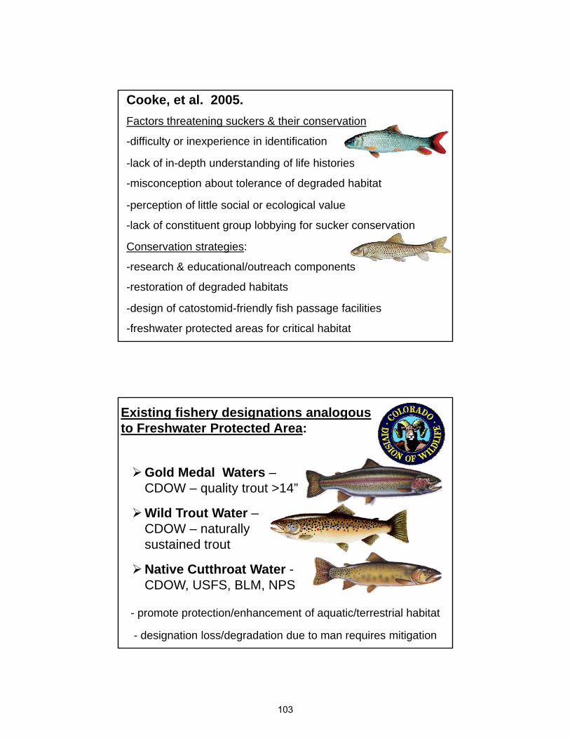
Cooke, et al. 2005. Factors threatening suckers & their conservation
-difficulty or inexperience in identification
-lack of in-depth understanding of life histories
-misconception about tolerance of degraded habitat
-perception of little social or ecological value
-lack of constituent group lobbying for sucker conservation
Conservation strategies:
-research & educational/outreach components
-restoration of degraded habitats
-design of catostomid-friendly fish passage facilities
-freshwater protected areas for critical habitat
Existing fishery designations analogous to Freshwater Protected Area:
- promote protection/enhancement of aquatic/terrestrial habitat
- designation loss/degradation due to man requires mitigation
Gold Medal Waters –CDOW – quality trout >14”
Native Cutthroat Water -CDOW, USFS, BLM, NPS
Wild Trout Water –CDOW – naturally sustained trout
103

Suski & Cooke. 2007. Conservation of aquatic resources through use of freshwater protected areas: opportunities & challenges. Biodivers. Cons. 16:2015-2029.
-FW environments experiencing alarming decline in biodiversity
-loss of FW biodiversity exceeds that in terrestrial & marine
-use freshwater protected areas (FPAs) to minimize disturbances & allow natural processes to govern populations & ecosystems
-similar practice used in marine & terrestrial environments
-have precedent for rare or spawning sport fish in freshwater
-slow adoption due to drainages, terminology & socio-economics
-additional FPAs needed for research & evaluation
-must address socio-economic obstacles & enforcement
Patrick J. Martinez, Aquatic Researcher Colorado Division of Wildlife, Grand Junction
March 2006
Designating Conservation Areas to Prioritize, Publicize, Popularize and Optimize Nonsalmonid Native Fish
Protection and Preservation
104

“Nonnative fish have wheels”
Illicit, Illegal, Unauthorized, Ill-conceived Fish Introductions
- undermines native fish conservation; circumvents oversight needed to foster compatibility of nonnative sport fish recreation & native sport fish conservation
- sport fishery damage, escapement, more illicit or invasive origins
105

Warmwater fish No. per decadeTotal
Family Species 1980 1990 2000Esocidae Northern pike 2 5 4 11
Centrarchidae
Bluegill 1 1 2
Green sunfish 1 1 2
Black crappie 4 2 6
Largemouth bass 1 1
Smallmouth bass 1 1 4 6
Percidae Yellow perch 4 2 6
Walleye 5 2 7
Total 8 10 17 14 41
Number per year 1.0 1.7 2.0 1.4
Illicit Introductions of Nonnative Sport Fish in Western CO
CO-WY AFS Resolution on Curtailing Illegal Fish IntroductionsWHEREAS, fisheries professionals have a public trust responsibility to
conserve & protect all aquatic wildlife & their habitats for future generations;&
WHEREAS, deliberate, unauthorized & illegal fish introductions are adversely impacting aquatic resources;
&WHEREAS, illegal introductions often impede ongoing mgmt. & restoration
efforts, many times at great expense in terms of agency time & public resources;
&WHEREAS, these introductions can have enormous & unmitigatible economic
& ecological impacts;&
WHEREAS, there continue to be new introductions in spite of ongoing education & regulatory efforts;
&WHEREAS, current approaches are clearly not providing adequate protection
for aquatic wildlife;&
WHEREAS, the American Fisheries Society (AFS) is the leading organization of fisheries professionals; now,
106

CO-WY AFS Resolution on Curtailing Illegal Fish Introductions (con’t)
THEREFORE, BE IT RESOLVED, that CO-WY AFS shall establish a committee to identify effective strategies already in use & to devise new approaches to curtail illegal fish introductions; the committee will convene workshops, workgroups, special symposia or any other tools & methods they deem appropriate; they should seek insight within the Chapter, the Western Div. & the Parent Society of the AFS as they work on this difficult problem;
&BE IT FURTHER RESOLVED, that the CO-WY AFS will work with fisheries management agencies to implement solutions & urges agency administrators to support the efforts of this CO-WY AFS committee;
&BE IT FURTHER RESOLVED, that the CO-WY AFS urges fisheries management agencies to immediately & aggressively expand their current efforts & adopt new regulatory, education & outreach, & management strategies to curtail illegal stocking;
&BE IT FURTHER RESOLVED, that this resolution be sent to the: Directors of the CDOW & WG&FD; Statewide Aquatic Manager, CDOW; & Chief of Fisheries, WG&FD
Adopted by CO-WY AFS 17 August 2007
Illicit fish stocking:
- sport fishery damage
- economic impacts
- threat to native fishes
Strategies to combat illicit fish stocking - near term :
- WLC policy
- no bag limits in specific waters
- no special regulations
- increase penalties
- no Master Angler or State Record recognition
Undesirable Aquatic Species Management (Draft CDOW White Paper)
107

Strategies to combat illicit fish stocking - long term :
Public education
- threat to native and sport fish resources – dual mission
- ecological, ethical & economic costs = “Big Deal”
- Aquatic Project Wild – “no free lunch” message
Public information
- explain different fish management or E vs W (T&E) CO
- Angler Roundtables for public info. & involvement
- Fishing Brochure (regs) – stress unauthorized stocking
- CDOW Fishing Report – dual mgmt. & fishing diversity
Undesirable Aquatic Species Management (Draft CDOW White Paper)
Strategies to combat illicit fish stocking - long term (con’t):
Aquatic research/management
- Invasive Species Coordinator
- survey strategies used in other states
- review “release of aquatic wildlife” regulations
- a priori must-kill regulations
- investigate mechanical removal of unwanted species
- investigate chemical reclamation of unwanted species
- scientifically ID reservoir for predator management
- stock sterile or hybrid nonnative sport fish
Undesirable Aquatic Species Management (Draft CDOW White Paper)
108

Strategies to combat illicit fish stocking - long term (con’t):
Aquatic research/management
- Invasive Species Coordinator
- survey strategies used in other states
- review “release of aquatic wildlife” regulations
- a priori must-kill regulations
- investigate mechanical removal of unwanted species
- investigate chemical reclamation of unwanted species
- scientifically ID reservoir for predator management
- stock sterile or hybrid nonnative sport fish
- modify Stocking Procedures for UCRB
Undesirable Aquatic Species Management (Draft CDOW White Paper)
Undesirable Aquatic Species Management (Draft CDOW White Paper)
Strategies to combat illicit fish stocking - long term (con’t) :
Law Enforcement
- hire investigator specifically for aquatic issues
- Operation Game Thief Reward
- prepared responses for blogs inciting illicit stocking
- implement forensic use of water/otolith microchemisty
- publicize law enforcement techniques as deterrent
Coordination with others
- USFWS, academia, scientific organizations, states
- CSU, AFS, AFWA help spread message
- WD Task Force, VHS implications
109
110
APPENDIX D
POWERPOINT PRESENTATION
INVASIVE & ILLICITLY INTRODUCED AQUATIC SPECIES: PERSPECTIVES FROM THE UPPER COLORADO RIVER
BASIN
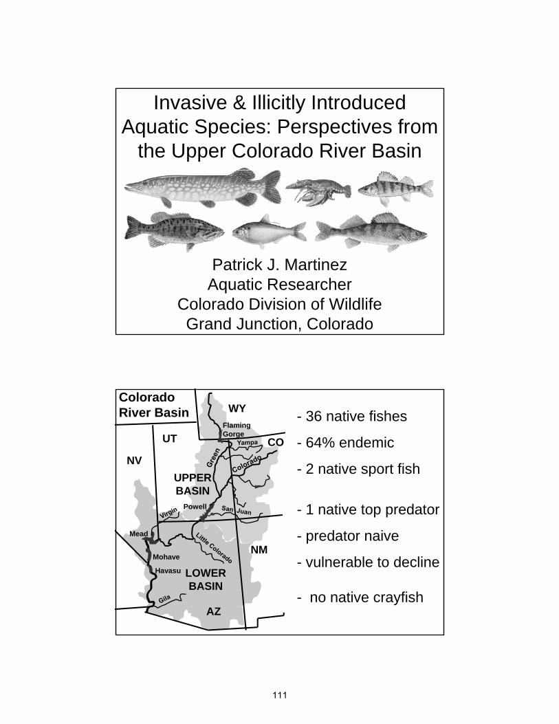
Invasive & Illicitly Introduced Aquatic Species: Perspectives from
the Upper Colorado River Basin
Patrick J. Martinez Aquatic Researcher
Colorado Division of Wildlife Grand Junction, Colorado
Colorado River Basin WY
COUT
NV
Flaming Gorge
- 36 native fishes
- 64% endemic
- 2 native sport fish
NM
Powell
Mead
UPPER BASIN
2 native sport fish
- 1 native top predator
- predator naive
AZ
Mohave
Havasu LOWER BASIN
- vulnerable to decline
- no native crayfish
111

Native Fishes
WYCO
UTFlaming Gorge
Upper Basin S
SCO
Gunnison
Blue
E
3
3
3
Powell
Blue Mesa
AZ NM
E
E E
P
Upper Basin Nonnative Aquatic Species
P
PP P
P
PP
P P
112

“Battle Against Extinction”- UCRB Endangered Fish Recovery Program: habitat,
flow, endangered fish monitoring & stocking, nonnative fish control
d li i d d & ti fi h- declines in endangered & native fishes
- expansion of nonnative aquatic species
- nonnative fish reduce biodiversity: predation, competition & hybridization
- nonnative vs. native fish abundance inversely related
- nonnative fish equal, if not greater, threat to native fishes than habitat degradation
(Schade & Bonar 2006 NAJFM)
WY
COUT
Flaming Gorge
Critical Habitat
StateCO X X X XCO
Gunnison
BlueUPPER BASIN
CO X X X X
NM X X
UT X X X X
River GR X X X X
YA X X X X
Powell
Blue Mesa
BASIN
AZ NM
WH X X
CO X X X X
GU X X
SJ X Xselective native fish passages
113

abun
danc
era
do p
ikem
inno
w a
G Ri B i
(Bestgen et al. 2007. TAFS)
Col
or Green River Basin
Procedures for Stocking Nonnative Fish Species in the Upper Colorado River Basin
- stocking consistent with endangered fish recovery
- provide & enhance recreational fishing
- reduce nonnative fish accessing critical habitat
- nonnative fishes continue to be stocked for angling
- native fish preservation must consider implications of stocking nonnative sport fish
- eliminate or mitigate nonnative fish impacts(Schade & Bonar. 2006. NAJFM)
114

- Invasive species: nonnative aquatic species that spread, persist or proliferate in aquatic habitats (may originate from authorized or illicit introduction)
Two major potential problems with some introduced or stocked aquatic species
- Illicit introduction: inadvertent, intentional, illegal or otherwise unauthorized movement of nonnative aquatic species to a new location (may become invasive species)
originate from authorized or illicit introduction)
- either dispersal mechanism may undermine Stocking p y gProcedures, nonnative fish control, selective fish passages, native fish preservation, reintroduction or recovery, freshwater protected areas & sport fisheries
- angling diversity vs. biological diversity
Warmwater sport fish No. per decadeTotal
Family Species 1980 1990 2000Esocidae Northern pike 2 4 5 11
Illicit Introductions of Nonnative Fish in Western CO
p
Centrarchidae
Bluegill 1 1 2
Green sunfish 1 1 2
Black crappie 3 2 5
Largemouth bass 1 1
Smallmouth bass 1 1 5 7Percidae Yellow perch 1 4 2 7
Walleye 4 2 6Total 8 10 15 16 41
Number per year 1.0 1.5 2.0 1.5
115

River Northern Yellow Smallmouth Walleye
- nonnative fish species have performed differently in rivers
River pike perch bass Walleye
Colorado rare rare common rare
Gunnison rare none none none
Green common none abundant rare
Yampa abundant none abundant rare
- illicitly stocked fish also affect reservoir fisheries
WY
UT
Elkh dDinosaur
CO
- northern pike introduced into Elkhead Reservoir in 1977
critical habitatnorthern pike
10 mi. Stagecoach Reservoir
Elkhead Reservoir
CRAIG
Dinosaur National Monument
MAYBELL
STEAMBOAT SPRINGS
RM 0 RM 140NCatamount Reservoir
- prey on native fishes; pike being removed in UCRB rivers
- invasively established up- & downstream by mid-1980s
- illicitly introduced into Stagecoach Reservoir in 1994
116

- CDOW. 2005. trout (70%); walleye (9%); bass (6%)
- CDOW. 2006. trout (78%); walleye (6%); bass (3%)
Is there high angler demand for northern pike?
- prey on long-lived adult native fishes (40-70% body-length)
State record : 2006 46.5-inches, 30.7- pounds
Stagecoach Reservoir
Stagecoach Reservoir Fishery- managed with subcatchable salmonids 1980s–1990s
- fishery succumbed to pike predation in late-1990s
- pike attract some anglers – Park use declinespike attract some anglers Park use declines
- stock >12-inch catchable trout to avoid predation
- more expensive, reduce hatchery space & fewer trout
- Park use rebounded, starving pike < 30-inch
- walleye illicitly introduced early-2000s
- northern pike invasive & illicitly moved
- pike affect native, coldwater & warmwater fishes
117

Crawford improvements should have assisted trout (Daily Sentinel 27 May 2003)Where are the trout in Crawford Reservoir?
Crawford a poor lake for trout, but great for other species (Daily Sentinel 4 June 2003)In response to the recent letter to the editor….pike were illegally planted
….a fisherman, will see one of the prettiest lakes… a cesspool of fish.
I called the hatchery… they were instructed not to put any trout in the reservoir the last two or three years because of the pike. Where did the pike come from?
Trout …never grow large due to oxygen depletion coming from the high temperatures.
Pike impacted the perch to the point where the crappie now have a chance to expand. The perch are running at least two to three inches longer.p
….with rainbow and brown troutone could catch their limit in a few hours… The trout thrived
We need to barrage elected officials to try to get our lake back.
g
….fish such as pike, perch, crappie and catfish, are better eating than trout.
I love to chase trophy class fish …I have turned loose three pike over 40 inches and exceeding 20 pounds.
Yellow Perch in Western Colorado- primarily illicit introductions; provide panfishing
- not highly invasive in UCRB rivers
Blue Mesa Reservoir – perch illicitly stocked late-1990s
- problematic in large coldwater reservoirs
- prey on invertebrates & kokanee fry
- increase angler participation or harvest?
- angler contention that pike improve panfishing?
- pike prey on larger perch (Paukert & Willis. 2003. NAJFM)
- angling diversity, fishery cost, angler retention & recruitment
118

WY
UT
Di
CO
critical habitat - smallmouth bass pike introduced into Elkhead Reservoir late-1970ssmallmouth bass
10 mi. Stagecoach Reservoir
Elkhead Reservoir
CRAIG
Dinosaur National Monument
MAYBELL
STEAMBOAT SPRINGS
RM 0 RM 140NCatamount Reservoir
- concurrently, small-bodied fish, including natives, declined
- verile crayfish also increase; drought & higher temperatures
- invasively established mid-1990s, increased in 2000s
5
20
25
30
35
Duffy
Sevens
Lily
Flannelmouth sucker Yampa R. 2001
15
20
25
30
35
%
Duffy
Sevens
Lily
Bluehead sucker Yampa R. 2001
8
10
12
14
16
18
%
Duffy
SevensLily
ampa
Bluehead sucker
Flannelmouth sucker
Roundtail chub
3-Species 2002
Flannelmouth sucker - Colorado R. 2001
8
0
2
Corn L
Clif ton
Bluehead sucker - Colorado R. 2001
8
10
12
14
Corn L
Clifton
Flannelmouth sucker - Colorado R. 2001
8
10
12
Corn L
Clif ton
0
5
0
6 8 10 12 14 16 18 20 22 24 26 28 30 32 34 36 38 40 42 44 46 48 50 52 54 56 58 60
length cm
0
5
10
6 8 10 12 14 16 18 20 22 24 26 28 30 32 34 36 38 40 42 44 46 48 50 52 54 56 58 60
length cm
0
2
4
6
9 10 11 12 13 14 15 16 17 18 19 20 21 22 23 24 25 26 27 28 29 30 31 32 33 34 35 36 37 38 39 40 41 42 43 44 45 46 47 48
length cm
rado
Ya
0
2
4
6
1 3 5 7 9 11 13 15 17 19 21 23 25 27 29 31 33 35 37 39 41 43 45 47 49 51 53 55
length cm
0
2
4
6
9 10 11 12 13 14 15 16 17 18 19 20 21 22 23 24 25 26 27 28 29 30 31 32 33 34 35 36 37 38 39 40 41 42 43 44 45 46 47
length cm
%
0
2
4
6
1 3 5 7 9 11 13 15 17 19 21 23 25 27 29 31 33 35 37 39 41 43 45 47 49 51 53 55
length cm
%
Col
or
150 300Total Length (mm)
150 300 150 300
119

WYUT
Flaming Gorge - illicit smallmouth bass stocking
Smallmouth bass
- smallmouth bass are recent invaders in UCRB rivers
- smallmouth bass from decades-old agency reservoir stocking
CO
Gunnison
Blue
in Gunnison basin reservoirs
40
60
80
t by
biom
ass
Smallmouth bass diet
s sh
Powell
Blue Mesa
AZ NMselective native fish passages
0
20
Colorado YampaP
erce
nt
Inse
cts
Fish
Cra
yfi s
(Johnson et al. in press. NAJFM)
Verile Crayfish in Yampa River- not present in late-1970s (Carlson et al. 1979. CSU)
- in catfish & pike diets late-1980s; crayfish origin unknown
67 000 90 000/h 80 144 k /h id 2000
- bass maintain condition despite reduction of small-bodied fish
- 67,000-90,000/ha, 80-144 kg/ha mid-2000s
- compete with flannelmouth sucker (Carpenter. 2005. EBoF)
reduction of small bodied fish
- smallmouth bass & crayfish = classic predator-prey combo
- crayfish likely accelerant for smallmouth bass
120

WYCO
UTFlaming Gorge
- invasive walleye have spotty distribution in UCRB rivers
Walleye
t i i h i d
- present in some UCRB reservoirs > 30 years
CO
Gunnison
Blue
- classic predator-prey combo in eastern Colorado reservoirs = walleye & gizzard shad
- capture in rivers has increased
Powell
Blue Mesa
AZ NMselective native fish passages
- could gizzard shad become accelerant for walleye in rivers?
Gizzard shadWY
COUT
NV
Flaming Gorge - hitchhiked with largemouth
bass from IDNFH, TX, to Morgan Lake, NM, in 1996
NM
Powell
Mead
UPPER BASIN
- invaded San Juan River by 2000 & Lake Powell by 2002 (Mueller & Brooks. 2004. WNAN )
- Green River, 2005 & Colorado & Gunnison Rivers, 2006
AZ
Mohave
Havasu LOWER BASIN
- Green River,CO & Lake Mead, AZ 2007 (Finney & Fuller. in prep. WNAN)
- must check all hatchery shipments into UCRB
121

Concluding remarks- sport fisheries & native fishes: “Battle Against Extinction”
- expansion in few years to decades, not all species the same
- undermine native fish conservation measures & investments
- salmonids compatible with UCRB “big-river” native fishes
- nonnative warmwater sport fishes: angling- vs. bio-diversity
- pike & perch can be detrimental to salmonid fisheries
p g g y
- angler satisfaction, recruitment & retention vs. fishery costs
- predation on long-lived adult native fishes
- pike benefits to pan fisheries dubious or deleterious
Concluding remarks (continued)
- crayfish likely accelerant for smallmouth bass in UCRB rivers
- smallmouth bass highly invasive in UCRB rivers
- new species in UCRB rivers; may trigger unforseen expansions
- point sources may be difficult to identify & control; dispersal often up- & downstream; mitigation expensive or impossible
- invasive & illicit pathways must receive greater preventive, ecological, administrative, hatchery & enforcement attention
122

Acknowledgements
Jim Brooks, Bob Burdick, Sam Finney – USFWS
Billy Atkinson, Dan Kowalski, Mike Japhet – CDOW
Brett Johnson, John Hawkins - CSU
123