École doctorale mathÉmatiques, sciences …...a novel semantic appracho for understanding the...
TRANSCRIPT

ÉCOLE DOCTORALE "MATHÉMATIQUES, SCIENCES DEL’INFORMATION ET DE L’INGÉNIEUR"
Laboratoire ICube - UMR7357
ÉCOLE DOCTORALE "SCIENCES DE GESTION"
Laboratoire LARODEC - LR01ES02
Thèse en cotutelle internationale présentée par :
Ali AYADI
soutenue le : 28 septembre 2018
pour obtenir le grade de : Docteur de l’Université de Strasbourg et l’Université de Tunis
Discipline/Spécialité : Informatique
Semantic approaches for the meta-optimization of complexbiomolecular networks
Approches sémantiques pour la méta-optimisation des réseauxbiomoléculaires complexes
THÈSE dirigée par :
Mme Cecilia ZANNI-MERK Professeur, INSA Rouen, Université de Normandie, LITISMme Saoussen KRICHEN Professeur, ISG de Tunis, Université de Tunis, LARODEC
RAPPORTEURS :
Mme Claudia FRYDMAN Professeur, Université d’Aix-Marseille, LISMme Lina SOUALMIA Maîtres de conférences HDR, Université de Rouen, LITIS
Autres membres du jury :
M. Edward SZCZERBICKI Professeur, University of Newcastle AustraliaM. François de BERTRAND de BEUVRON Maîtres de conférences, INSA Strasbourg, ICubeM. Olivier POCH Directeur de recherches, Université de Strasbourg, ICube


Acknowledgements
First of all, I would like to express my gratitude to my PhD advisers, Cecilia ZANNI-MERK, Françoisde BERTRAND de BEUVRON, Saoussen KRICHEN and Julie THOMPSON who have been activelyinterested in my work. I would like to thank them as well for encouraging me and for allowing me togrow as a research scientist.
I deeply acknowledge the extraordinary and meticulous support of Cecilia ZANNI-MERK for the freeexchange of ideas, constructive criticism, guidance, encouragement and moral support throughout thework. I am truly thankful for helping me achieve personal and professional goals.
Special thanks to François de BERTRAND de BEUVRON who graciously supported me with thesiscomments and for his critical knowledge feedback that enriched my thesis with appropriate context, aswell as for his encouragement and moral support.
I am also thankful to Saoussen KRICHEN for allowing me the opportunity to pursue a career inresearch, and for her encouragements.
In addition, I am very thankful to Julie THOMPSON for providing biological data and her help invalidating the experimental results presented in this thesis.
Besides my advisers, I am very thankful to Claudia FRYDMAN and Lina SOUALMIA for acceptingto read and review my thesis manuscript.
I gratefully acknowledge Olivier POCH and Edward SZCZERBICKI for accepting to be members ofmy thesis committee.
I would also like to thank my mid-thesis committee, Claudia FRYDMAN and Olivier POCH, for theirinsightful comments and encouragement.
I am thankful to thank the University of Strasbourg and the University of Tunis for funding my PhDstudies. In addition, I would like to thank ICube administrative sta�.
Lastly, I would like to thank my parents, my sister Zouhayra AYADI, my �ancee Eya MERSNI, andmy close friends for their unfailing support and endless inspiration throughout these past three years ofmy PhD studies. In particular, Abdoul-Djawadou SALAOU for his help in validating my experimentalresults.
i

ii

List of publications
The work of this thesis is based on the following publications:International peer-reviewed conferences
• A. Ayadi, C. Zanni-Merk, F. de Bertrand de Beuvron, S. Krichen. A multi-objective method foroptimizing the transittability of complex biomolecular networks, 22th International Conference onKnowledge-Based and Intelligent Information & Engineering Systems, Belgrade, Serbia, ProcediaComputer Science, septembre 2018.
• A. Ayadi, C. Zanni-Merk, F. de Bertrand de Beuvron, S. Krichen. A multi-objective mathematicalmodel for the optimization of the transittability of complex biomolecular network, 22th InternationalConference on Knowledge-Based and Intelligent Information & Engineering Systems, Belgrade,Serbia, Procedia Computer Science, septembre 2018.
• A. Ayadi, C. Zanni-Merk, F. de Bertrand de Beuvron, S. Krichen. Ontological reasoning for under-standing the behaviour of complex biomolecular networks. In : Computer Systems and Applications(AICCSA), 2017 IEEE/ACS 14th International Conference on. IEEE, 2017. p. 1486-1493.
• A. Ayadi, C. Zanni-Merk, F. de Bertrand de Beuvron, S. Krichen. BNO: An ontology for describingthe behaviour of complex biomolecular networks, 21th International Conference on Knowledge-Basedand Intelligent Information & Engineering Systems, Marseille, France, Procedia Computer Science,septembre 2017, doi:10.1016/j.procs.2017.08.159.
• A. Ayadi, C. Zanni-Merk, F. de Bertrand de Beuvron, S. Krichen. CBNSimulator: a simulator toolfor understanding the behaviour of complex biomolecular networks using discrete time simulation,21th International Conference on Knowledge-Based and Intelligent Information & Engineering Sys-tems, Marseille, France, page 8, Procedia Computer Science, avril 2017, doi:10.1016/j.procs.2017.08.157.
• A. Ayadi, C. Zanni-Merk, F. de Bertrand de Beuvron. Understanding the Behaviour of ComplexBiomolecular Networks by Combining Logical and Semantic Modeling, 9th International ConferenceSemantic Web Applications and Tools for Life Sciences, Amsterdam, Netherlands, page 12, Volume1795, décembre 2016.
• A. Ayadi, C. Zanni-Merk, F. de Bertrand de Beuvron. Qualitative Reasoning for Understanding theBehaviour of Complex Biomolecular Networks, the 8th International Joint Conference on KnowledgeDiscovery, Knowledge Engineering and Knowledge Management - KEOD 2016, Porto, Portugal,pages 144-149, Volume 2, n◦ 978-989-758-203-5, octobre 2016, doi:10.5220/0006065901440149.
• A. Ayadi, C. Zanni-Merk, F. de Bertrand de Beuvron, S. Krichen. Logical Semantic Modelingof Complex Biomolecular Networks, Knowledge-Based and Intelligent Information & EngineeringSystems: Proceedings of the 20th International Conference KES-2016, York, United Kingdom, pages475 - 484, Procedia Computer Science, Volume 96, septembre 2016, doi:http://dx.doi.org/10.1016/j.procs.2016.08.108.
• A. Ayadi, F. de Bertrand de Beuvron, C. Zanni-Merk, J. Thompson. Formalisation des réseauxbiomoléculaires complexes, EGC 2016 � 16èmes Journées Francophones "Extraction et Gestiondes Connaissances", Reims, France, Revue des Nouvelles Technologies de l'Information, VolumeRNTI-E-30, janvier 2016.
iii

International peer-reviewed journals
• A. Ayadi, C. Zanni-Merk, F. de Bertrand de Beuvron, S. Krichen and Julie Thompson. A multi-objective method for optimizing the transittability of complex biomolecular networks, IEEE Trans-actions on Biomedical Engineering (submitted July 2018).
• A. Ayadi, C. Zanni-Merk, F. de Bertrand de Beuvron, S. Krichen and Julie Thompson. A novelsemantic approach for understanding the dynamic behaviour of biological networks, InternationalJournal of Kinesiology and Sport Science (submitted June 2018).
• A. Ayadi, C. Zanni-Merk, F. de Bertrand de Beuvron, S. Krichen and Julie Thompson. BNO -an ontology for understanding the transittability of complex biomolecular networks, Journal of WebSemantics (submitted November 2017).
iv

Contents
Acknowledgements i
List of publications iii
List of Figures xiii
List of tables xv
General introduction 1Biological and scienti�c context . . . . . . . . . . . . . . . . . . . . . . . . . . . . . . . . . . . . 1Aims and objectives . . . . . . . . . . . . . . . . . . . . . . . . . . . . . . . . . . . . . . . . . . 2Contributions and �elds of research concerned . . . . . . . . . . . . . . . . . . . . . . . . . . . . 4Thesis outline . . . . . . . . . . . . . . . . . . . . . . . . . . . . . . . . . . . . . . . . . . . . . . 4
I State-of-the-Art 7
1 Biological environment: from molecular biology to systems biology 91.1 Introduction . . . . . . . . . . . . . . . . . . . . . . . . . . . . . . . . . . . . . . . . . . . . 101.2 Biological background . . . . . . . . . . . . . . . . . . . . . . . . . . . . . . . . . . . . . . 10
1.2.1 Deoxyribonucleic acid (DNA) . . . . . . . . . . . . . . . . . . . . . . . . . . . . . . 101.2.2 Ribonucleic acid (RNA) . . . . . . . . . . . . . . . . . . . . . . . . . . . . . . . . . 101.2.3 Proteins . . . . . . . . . . . . . . . . . . . . . . . . . . . . . . . . . . . . . . . . . . 111.2.4 Metabolites . . . . . . . . . . . . . . . . . . . . . . . . . . . . . . . . . . . . . . . . 111.2.5 Gene expression . . . . . . . . . . . . . . . . . . . . . . . . . . . . . . . . . . . . . 12
1.3 From molecular biology to systems biology . . . . . . . . . . . . . . . . . . . . . . . . . . . 141.4 Complex biomolecular networks . . . . . . . . . . . . . . . . . . . . . . . . . . . . . . . . . 141.5 Transittability of complex biomolecular networks . . . . . . . . . . . . . . . . . . . . . . . 161.6 Summary . . . . . . . . . . . . . . . . . . . . . . . . . . . . . . . . . . . . . . . . . . . . . 17
2 Modelling in systems biology 192.1 Introduction . . . . . . . . . . . . . . . . . . . . . . . . . . . . . . . . . . . . . . . . . . . . 202.2 Major properties and dimensions of modelling . . . . . . . . . . . . . . . . . . . . . . . . . 20
2.2.1 Discrete vs Continuous vs Hybrid models . . . . . . . . . . . . . . . . . . . . . . . 202.2.1.1 Discrete models . . . . . . . . . . . . . . . . . . . . . . . . . . . . . . . . 202.2.1.2 Continuous models . . . . . . . . . . . . . . . . . . . . . . . . . . . . . . . 202.2.1.3 Hybrid models . . . . . . . . . . . . . . . . . . . . . . . . . . . . . . . . . 20
2.2.2 Quantitative vs Qualitative models . . . . . . . . . . . . . . . . . . . . . . . . . . . 212.2.2.1 Quantitative models: . . . . . . . . . . . . . . . . . . . . . . . . . . . . . 212.2.2.2 Qualitative models: . . . . . . . . . . . . . . . . . . . . . . . . . . . . . . 21
2.3 Overview of the existing mathematical models in systems biology . . . . . . . . . . . . . . 212.3.1 Boolean models . . . . . . . . . . . . . . . . . . . . . . . . . . . . . . . . . . . . . . 212.3.2 Logical models . . . . . . . . . . . . . . . . . . . . . . . . . . . . . . . . . . . . . . 212.3.3 Petri nets models . . . . . . . . . . . . . . . . . . . . . . . . . . . . . . . . . . . . . 222.3.4 Bayesian network models . . . . . . . . . . . . . . . . . . . . . . . . . . . . . . . . 22
v
CONTENTS
2.3.5 Graphical Gaussian models . . . . . . . . . . . . . . . . . . . . . . . . . . . . . . . 222.3.6 Di�erential equation models . . . . . . . . . . . . . . . . . . . . . . . . . . . . . . . 232.3.7 Cellular automata models . . . . . . . . . . . . . . . . . . . . . . . . . . . . . . . . 232.3.8 Agent-based models . . . . . . . . . . . . . . . . . . . . . . . . . . . . . . . . . . . 23
2.4 Comparison among these modelling formalisms . . . . . . . . . . . . . . . . . . . . . . . . 242.5 Thesis contribution in this �eld . . . . . . . . . . . . . . . . . . . . . . . . . . . . . . . . . 262.6 Summary . . . . . . . . . . . . . . . . . . . . . . . . . . . . . . . . . . . . . . . . . . . . . 26
3 Ontologies in systems biology 273.1 Introduction . . . . . . . . . . . . . . . . . . . . . . . . . . . . . . . . . . . . . . . . . . . . 283.2 Concept of Ontology . . . . . . . . . . . . . . . . . . . . . . . . . . . . . . . . . . . . . . . 283.3 Ontology components . . . . . . . . . . . . . . . . . . . . . . . . . . . . . . . . . . . . . . 283.4 Typologies of ontologies . . . . . . . . . . . . . . . . . . . . . . . . . . . . . . . . . . . . . 29
3.4.1 According to the object of generality . . . . . . . . . . . . . . . . . . . . . . . . . . 293.4.2 According to the level of detail . . . . . . . . . . . . . . . . . . . . . . . . . . . . . 293.4.3 According to the level of formality . . . . . . . . . . . . . . . . . . . . . . . . . . . 30
3.5 Ontology building: methodologies, formalisms, languages and tools . . . . . . . . . . . . . 303.5.1 Ontology engineering methodologies . . . . . . . . . . . . . . . . . . . . . . . . . . 30
3.5.1.1 Uschold and King's method . . . . . . . . . . . . . . . . . . . . . . . . . . 303.5.1.2 SENSUS method . . . . . . . . . . . . . . . . . . . . . . . . . . . . . . . . 303.5.1.3 METHONTOLOGY method . . . . . . . . . . . . . . . . . . . . . . . . . 313.5.1.4 The Stanford's method . . . . . . . . . . . . . . . . . . . . . . . . . . . . 31
3.5.2 Types of formalisms . . . . . . . . . . . . . . . . . . . . . . . . . . . . . . . . . . . 313.5.3 Languages . . . . . . . . . . . . . . . . . . . . . . . . . . . . . . . . . . . . . . . . . 32
3.5.3.1 KIF . . . . . . . . . . . . . . . . . . . . . . . . . . . . . . . . . . . . . . . 323.5.3.2 KL-ONE . . . . . . . . . . . . . . . . . . . . . . . . . . . . . . . . . . . . 323.5.3.3 RDF and RDF Schema . . . . . . . . . . . . . . . . . . . . . . . . . . . . 323.5.3.4 DAML-ONT . . . . . . . . . . . . . . . . . . . . . . . . . . . . . . . . . . 333.5.3.5 DAML + OIL . . . . . . . . . . . . . . . . . . . . . . . . . . . . . . . . . 333.5.3.6 OWL . . . . . . . . . . . . . . . . . . . . . . . . . . . . . . . . . . . . . . 333.5.3.7 OCL . . . . . . . . . . . . . . . . . . . . . . . . . . . . . . . . . . . . . . 34
3.5.4 Editing tools . . . . . . . . . . . . . . . . . . . . . . . . . . . . . . . . . . . . . . . 343.6 Ontology reasoning . . . . . . . . . . . . . . . . . . . . . . . . . . . . . . . . . . . . . . . . 35
3.6.1 Semantic Web Rule Language . . . . . . . . . . . . . . . . . . . . . . . . . . . . . . 353.6.2 SWRL sytax . . . . . . . . . . . . . . . . . . . . . . . . . . . . . . . . . . . . . . . 353.6.3 Reasoning systems for description logic . . . . . . . . . . . . . . . . . . . . . . . . 35
3.7 Overview of existing ontology applications in systems biology . . . . . . . . . . . . . . . . 353.8 Comparison among these bio-ontologies . . . . . . . . . . . . . . . . . . . . . . . . . . . . 363.9 Thesis contribution in this �eld . . . . . . . . . . . . . . . . . . . . . . . . . . . . . . . . . 363.10 Summary . . . . . . . . . . . . . . . . . . . . . . . . . . . . . . . . . . . . . . . . . . . . . 36
4 Simulation tools in systems biology 394.1 Introduction . . . . . . . . . . . . . . . . . . . . . . . . . . . . . . . . . . . . . . . . . . . . 404.2 Principles of simulation . . . . . . . . . . . . . . . . . . . . . . . . . . . . . . . . . . . . . 40
4.2.1 De�nition . . . . . . . . . . . . . . . . . . . . . . . . . . . . . . . . . . . . . . . . . 404.2.2 Relation between modelling and simulation concepts . . . . . . . . . . . . . . . . . 404.2.3 Uses of simulation . . . . . . . . . . . . . . . . . . . . . . . . . . . . . . . . . . . . 414.2.4 Levels of abstraction . . . . . . . . . . . . . . . . . . . . . . . . . . . . . . . . . . . 41
4.3 Overview of existing simulation tools in systems biology . . . . . . . . . . . . . . . . . . . 414.3.1 Mathematical and population-based simulation . . . . . . . . . . . . . . . . . . . . 424.3.2 Individual-based simulation . . . . . . . . . . . . . . . . . . . . . . . . . . . . . . . 42
4.3.2.1 Cellular Automata . . . . . . . . . . . . . . . . . . . . . . . . . . . . . . . 424.3.2.2 Multi-Agent Systems . . . . . . . . . . . . . . . . . . . . . . . . . . . . . 424.3.2.3 Potts model . . . . . . . . . . . . . . . . . . . . . . . . . . . . . . . . . . 434.3.2.4 Lattice gas automata . . . . . . . . . . . . . . . . . . . . . . . . . . . . . 43
4.3.3 Computational simulation platforms . . . . . . . . . . . . . . . . . . . . . . . . . . 43
vi

CONTENTS
4.3.3.1 Simulation standard . . . . . . . . . . . . . . . . . . . . . . . . . . . . . . 434.3.3.2 Simulation tools . . . . . . . . . . . . . . . . . . . . . . . . . . . . . . . . 44
4.3.4 Discrete Event System Speci�cation . . . . . . . . . . . . . . . . . . . . . . . . . . 454.3.4.1 Basic Models . . . . . . . . . . . . . . . . . . . . . . . . . . . . . . . . . . 454.3.4.2 Coupled models . . . . . . . . . . . . . . . . . . . . . . . . . . . . . . . . 454.3.4.3 Bene�ts of DEVS . . . . . . . . . . . . . . . . . . . . . . . . . . . . . . . 45
4.4 Comparison among these simulation tools and platforms . . . . . . . . . . . . . . . . . . . 464.5 Thesis contribution in this �eld . . . . . . . . . . . . . . . . . . . . . . . . . . . . . . . . . 474.6 Summary . . . . . . . . . . . . . . . . . . . . . . . . . . . . . . . . . . . . . . . . . . . . . 49
5 Optimization tools in systems biology 515.1 Introduction . . . . . . . . . . . . . . . . . . . . . . . . . . . . . . . . . . . . . . . . . . . . 525.2 Optimization problem: de�nition and basic concepts . . . . . . . . . . . . . . . . . . . . . 52
5.2.1 De�nition . . . . . . . . . . . . . . . . . . . . . . . . . . . . . . . . . . . . . . . . . 525.2.2 The objective function . . . . . . . . . . . . . . . . . . . . . . . . . . . . . . . . . . 535.2.3 The vector of decision variables . . . . . . . . . . . . . . . . . . . . . . . . . . . . . 535.2.4 Constraints and delimitation of the research space . . . . . . . . . . . . . . . . . . 535.2.5 The di�erent types of optimum points . . . . . . . . . . . . . . . . . . . . . . . . . 53
5.2.5.1 Local maximum and minimum . . . . . . . . . . . . . . . . . . . . . . . . 545.2.5.2 Global maximum and minimum . . . . . . . . . . . . . . . . . . . . . . . 54
5.3 Classi�cation of optimization problems . . . . . . . . . . . . . . . . . . . . . . . . . . . . . 545.4 Mono-objective optimization problem . . . . . . . . . . . . . . . . . . . . . . . . . . . . . 555.5 Multi-objective optimization problem . . . . . . . . . . . . . . . . . . . . . . . . . . . . . . 55
5.5.1 Dominance relation . . . . . . . . . . . . . . . . . . . . . . . . . . . . . . . . . . . . 565.5.2 Pareto-optimal solutions . . . . . . . . . . . . . . . . . . . . . . . . . . . . . . . . . 56
5.6 Optimization methods . . . . . . . . . . . . . . . . . . . . . . . . . . . . . . . . . . . . . . 575.6.1 The methods based on a metaheuristic approach . . . . . . . . . . . . . . . . . . . 57
5.6.1.1 Simulated annealing . . . . . . . . . . . . . . . . . . . . . . . . . . . . . . 585.6.1.2 Tabu search . . . . . . . . . . . . . . . . . . . . . . . . . . . . . . . . . . 585.6.1.3 Evolutionary Algorithms . . . . . . . . . . . . . . . . . . . . . . . . . . . 595.6.1.4 Ant colony . . . . . . . . . . . . . . . . . . . . . . . . . . . . . . . . . . . 61
5.7 Optimization problems in system biology . . . . . . . . . . . . . . . . . . . . . . . . . . . 625.7.1 Optimization in the design of optimal dynamic experiments . . . . . . . . . . . . . 625.7.2 Optimization in the parameter estimation in cell systems modelling . . . . . . . . 625.7.3 Optimization in biological network alignment . . . . . . . . . . . . . . . . . . . . . 635.7.4 Optimization of biochemical reaction networks . . . . . . . . . . . . . . . . . . . . 635.7.5 Optimization in the sequence alignment problem . . . . . . . . . . . . . . . . . . . 635.7.6 Optimization in inferring networks . . . . . . . . . . . . . . . . . . . . . . . . . . . 635.7.7 Optimization in the network controllability . . . . . . . . . . . . . . . . . . . . . . 64
5.8 Comparison among these optimization tools and problems . . . . . . . . . . . . . . . . . . 645.9 Thesis contribution in this �eld . . . . . . . . . . . . . . . . . . . . . . . . . . . . . . . . . 655.10 Summary . . . . . . . . . . . . . . . . . . . . . . . . . . . . . . . . . . . . . . . . . . . . . 65
II Contributions 67
6 Logical-based modelling of complex biomolecular networks 696.1 Introduction . . . . . . . . . . . . . . . . . . . . . . . . . . . . . . . . . . . . . . . . . . . . 706.2 Motivating example: the bacteriophage T4 gene 32 . . . . . . . . . . . . . . . . . . . . . . 706.3 System theory . . . . . . . . . . . . . . . . . . . . . . . . . . . . . . . . . . . . . . . . . . . 71
6.3.1 Complex systems . . . . . . . . . . . . . . . . . . . . . . . . . . . . . . . . . . . . . 716.3.2 System theory objectives . . . . . . . . . . . . . . . . . . . . . . . . . . . . . . . . 726.3.3 System theory axes . . . . . . . . . . . . . . . . . . . . . . . . . . . . . . . . . . . . 72
6.4 Logic-based approach for modelling biomolecular networks . . . . . . . . . . . . . . . . . . 736.4.1 Structural modelling . . . . . . . . . . . . . . . . . . . . . . . . . . . . . . . . . . . 746.4.2 Functional modelling . . . . . . . . . . . . . . . . . . . . . . . . . . . . . . . . . . . 75
vii

CONTENTS
6.4.3 Behavioural modelling . . . . . . . . . . . . . . . . . . . . . . . . . . . . . . . . . . 756.4.3.1 State of the network . . . . . . . . . . . . . . . . . . . . . . . . . . . . . . 766.4.3.2 Transition of the network state . . . . . . . . . . . . . . . . . . . . . . . . 766.4.3.3 Steering the network to a given state . . . . . . . . . . . . . . . . . . . . 766.4.3.4 Behaviour . . . . . . . . . . . . . . . . . . . . . . . . . . . . . . . . . . . . 77
6.5 Application to the motivating example . . . . . . . . . . . . . . . . . . . . . . . . . . . . . 776.6 Summary . . . . . . . . . . . . . . . . . . . . . . . . . . . . . . . . . . . . . . . . . . . . . 77
7 Semantic modelling of complex biomolecular networks 79
7.1 Introduction . . . . . . . . . . . . . . . . . . . . . . . . . . . . . . . . . . . . . . . . . . . . 807.2 Semantic approach for analysing the transittability of complex biomolecular networks . . 80
7.2.1 The global architecture . . . . . . . . . . . . . . . . . . . . . . . . . . . . . . . . . 807.2.2 The Gene Ontology (GO) . . . . . . . . . . . . . . . . . . . . . . . . . . . . . . . . 817.2.3 The Simple Event Model Ontology (SEMO) . . . . . . . . . . . . . . . . . . . . . . 827.2.4 The Time Ontology (TO) . . . . . . . . . . . . . . . . . . . . . . . . . . . . . . . . 827.2.5 The Biomolecular Network Ontology (BNO) . . . . . . . . . . . . . . . . . . . . . 827.2.6 The relations among these ontologies . . . . . . . . . . . . . . . . . . . . . . . . . . 82
7.3 The Biomolecular Network Ontology . . . . . . . . . . . . . . . . . . . . . . . . . . . . . . 837.3.1 Development . . . . . . . . . . . . . . . . . . . . . . . . . . . . . . . . . . . . . . . 837.3.2 The key concepts . . . . . . . . . . . . . . . . . . . . . . . . . . . . . . . . . . . . . 837.3.3 The major properties and data types . . . . . . . . . . . . . . . . . . . . . . . . . . 85
7.4 Application to the motivating example: the bacteriophage T4 gene 32 . . . . . . . . . . . 867.4.1 Instantiation of the BNO ontology . . . . . . . . . . . . . . . . . . . . . . . . . . . 867.4.2 SWRL rule-based reasoning . . . . . . . . . . . . . . . . . . . . . . . . . . . . . . . 87
7.4.2.1 Inhibition SWRL rule . . . . . . . . . . . . . . . . . . . . . . . . . . . . . 887.4.2.2 Activation SWRL rule . . . . . . . . . . . . . . . . . . . . . . . . . . . . . 887.4.2.3 Transcription SWRL rule . . . . . . . . . . . . . . . . . . . . . . . . . . . 897.4.2.4 Negative regulation SWRL rule . . . . . . . . . . . . . . . . . . . . . . . 91
7.4.3 Rule-based qualitative reasoner within MATLAB . . . . . . . . . . . . . . . . . . . 927.5 Summary . . . . . . . . . . . . . . . . . . . . . . . . . . . . . . . . . . . . . . . . . . . . . 93
8 Qualitative, discrete-event simulation of complex biomolecular networks 97
8.1 Introduction . . . . . . . . . . . . . . . . . . . . . . . . . . . . . . . . . . . . . . . . . . . . 988.2 Qualitative simulation model . . . . . . . . . . . . . . . . . . . . . . . . . . . . . . . . . . 98
8.2.1 Qualitative reasoning . . . . . . . . . . . . . . . . . . . . . . . . . . . . . . . . . . 988.2.2 Basic concepts . . . . . . . . . . . . . . . . . . . . . . . . . . . . . . . . . . . . . . 98
8.2.2.1 The causal graph . . . . . . . . . . . . . . . . . . . . . . . . . . . . . . . . 988.2.2.2 Quantitative variables & Quantity space . . . . . . . . . . . . . . . . . . 998.2.2.3 Operations and rules . . . . . . . . . . . . . . . . . . . . . . . . . . . . . 100
8.2.3 Application to the motivating example: the bacteriophage T4 gene 32 . . . . . . . 1008.2.3.1 The variables . . . . . . . . . . . . . . . . . . . . . . . . . . . . . . . . . . 1018.2.3.2 The causal graph . . . . . . . . . . . . . . . . . . . . . . . . . . . . . . . . 1018.2.3.3 The partition rules . . . . . . . . . . . . . . . . . . . . . . . . . . . . . . . 1018.2.3.4 The propagation rules . . . . . . . . . . . . . . . . . . . . . . . . . . . . . 1028.2.3.5 The simulation . . . . . . . . . . . . . . . . . . . . . . . . . . . . . . . . . 1028.2.3.6 The behaviour . . . . . . . . . . . . . . . . . . . . . . . . . . . . . . . . . 102
8.3 Discrete-event simulation model . . . . . . . . . . . . . . . . . . . . . . . . . . . . . . . . . 1038.3.1 Mapping the logical based modelling with the DEVS formalism . . . . . . . . . . . 1038.3.2 Discrete-event simulation algorithm . . . . . . . . . . . . . . . . . . . . . . . . . . 1038.3.3 Application to the motivating example: the bacteriophage T4 gene 32 . . . . . . . 105
8.4 Summary . . . . . . . . . . . . . . . . . . . . . . . . . . . . . . . . . . . . . . . . . . . . . 107
viii

CONTENTS
9 A multi-objective optimization method for solving the transittability of complexbiomolecular networks 1099.1 Introduction . . . . . . . . . . . . . . . . . . . . . . . . . . . . . . . . . . . . . . . . . . . . 1109.2 Problem statement . . . . . . . . . . . . . . . . . . . . . . . . . . . . . . . . . . . . . . . . 1109.3 Proposed multi-objective mathematical model . . . . . . . . . . . . . . . . . . . . . . . . . 111
9.3.1 Parameters . . . . . . . . . . . . . . . . . . . . . . . . . . . . . . . . . . . . . . . . 1119.3.2 Decision variables . . . . . . . . . . . . . . . . . . . . . . . . . . . . . . . . . . . . 1119.3.3 Objective functions . . . . . . . . . . . . . . . . . . . . . . . . . . . . . . . . . . . . 112
9.3.3.1 Minimizing the distance between the simulated �nal network state andthe desired network state . . . . . . . . . . . . . . . . . . . . . . . . . . . 112
9.3.3.2 Minimizing the number of external stimuli . . . . . . . . . . . . . . . . . 1139.3.3.3 Minimizing the cost of the external stimuli . . . . . . . . . . . . . . . . . 1139.3.3.4 Minimizing the number of target nodes . . . . . . . . . . . . . . . . . . . 1149.3.3.5 Minimizing the patient discomfort . . . . . . . . . . . . . . . . . . . . . . 114
9.3.4 Constraints . . . . . . . . . . . . . . . . . . . . . . . . . . . . . . . . . . . . . . . . 1159.4 Multi-objective optimization approach . . . . . . . . . . . . . . . . . . . . . . . . . . . . . 117
9.4.1 First step: search process . . . . . . . . . . . . . . . . . . . . . . . . . . . . . . . . 1179.4.1.1 NSGA-II algorithm overview . . . . . . . . . . . . . . . . . . . . . . . . . 1179.4.1.2 NSGA-II algorithm operation . . . . . . . . . . . . . . . . . . . . . . . . . 1189.4.1.3 Genetic algorithm implementation . . . . . . . . . . . . . . . . . . . . . . 118
9.4.2 Second step: decision making . . . . . . . . . . . . . . . . . . . . . . . . . . . . . . 1209.4.2.1 TOPSIS method overview . . . . . . . . . . . . . . . . . . . . . . . . . . . 1209.4.2.2 TOPSIS method operation . . . . . . . . . . . . . . . . . . . . . . . . . . 121
9.5 Summary . . . . . . . . . . . . . . . . . . . . . . . . . . . . . . . . . . . . . . . . . . . . . 122
III Experiments and discussion 123
10 Prototype: the CBNSimulator 12510.1 Introduction . . . . . . . . . . . . . . . . . . . . . . . . . . . . . . . . . . . . . . . . . . . . 12610.2 Aims of the CBNSimulator platform . . . . . . . . . . . . . . . . . . . . . . . . . . . . . . 12610.3 Overview of the CBNSimulator platform . . . . . . . . . . . . . . . . . . . . . . . . . . . . 12610.4 Development tools . . . . . . . . . . . . . . . . . . . . . . . . . . . . . . . . . . . . . . . . 12810.5 Experimental results . . . . . . . . . . . . . . . . . . . . . . . . . . . . . . . . . . . . . . . 128
10.5.1 Case study 1: the bacteriophage T4 gene 32 . . . . . . . . . . . . . . . . . . . . . . 12810.5.1.1 Description . . . . . . . . . . . . . . . . . . . . . . . . . . . . . . . . . . . 12810.5.1.2 Logical modelling . . . . . . . . . . . . . . . . . . . . . . . . . . . . . . . 12910.5.1.3 Semantic modelling . . . . . . . . . . . . . . . . . . . . . . . . . . . . . . 12910.5.1.4 Simulation under the CBNSimulator . . . . . . . . . . . . . . . . . . . . . 129
10.5.2 Case study 2: the control of the lifecycle of bacteriophage lambda . . . . . . . . . 12910.5.2.1 Description . . . . . . . . . . . . . . . . . . . . . . . . . . . . . . . . . . . 13010.5.2.2 Logic-based modelling . . . . . . . . . . . . . . . . . . . . . . . . . . . . . 13110.5.2.3 Semantic modelling . . . . . . . . . . . . . . . . . . . . . . . . . . . . . . 13110.5.2.4 Simulation under the CBNSimulator . . . . . . . . . . . . . . . . . . . . . 134
10.5.3 Case study 3: the p53-mediated DNA damage response network . . . . . . . . . . 13710.5.3.1 Description . . . . . . . . . . . . . . . . . . . . . . . . . . . . . . . . . . . 13710.5.3.2 Simulation under the CBNSimulator . . . . . . . . . . . . . . . . . . . . . 13810.5.3.3 Optimization of the p53-mediated DNA damage response network . . . . 141
10.6 Summary . . . . . . . . . . . . . . . . . . . . . . . . . . . . . . . . . . . . . . . . . . . . . 145
11 Discussion and evaluation 14911.1 Introduction . . . . . . . . . . . . . . . . . . . . . . . . . . . . . . . . . . . . . . . . . . . . 15011.2 Logic-based modelling discussion and evaluation . . . . . . . . . . . . . . . . . . . . . . . 15011.3 Ontology discussion and evaluation . . . . . . . . . . . . . . . . . . . . . . . . . . . . . . . 15211.4 Simulation discussion and evaluation . . . . . . . . . . . . . . . . . . . . . . . . . . . . . . 15611.5 Optimization discussion and evaluation . . . . . . . . . . . . . . . . . . . . . . . . . . . . 158
ix

CONTENTS
11.6 Summary . . . . . . . . . . . . . . . . . . . . . . . . . . . . . . . . . . . . . . . . . . . . . 159
General conclusion and future research 161Conclusion . . . . . . . . . . . . . . . . . . . . . . . . . . . . . . . . . . . . . . . . . . . . . . . 161Contributions . . . . . . . . . . . . . . . . . . . . . . . . . . . . . . . . . . . . . . . . . . . . . . 162Directions on future research . . . . . . . . . . . . . . . . . . . . . . . . . . . . . . . . . . . . . 164
Detailed abstract in French 167
Bibliography 179
x

List of Figures
1 Research laboratories and institutions in which this thesis has been conducted. . . . . . . 22 General architecture of our proposed platform. . . . . . . . . . . . . . . . . . . . . . . . . 33 The main structure of this thesis. . . . . . . . . . . . . . . . . . . . . . . . . . . . . . . . . 6
1.1 DNA and RNA structure (Image credit: Wikimedia). . . . . . . . . . . . . . . . . . . . . . 111.2 Protein structure (Image credit: Wikimedia). . . . . . . . . . . . . . . . . . . . . . . . . . 121.3 Examples of metabolites (Image credit: the West Coast Metabolomics Center). . . . . . . 131.4 The central drogma of life. . . . . . . . . . . . . . . . . . . . . . . . . . . . . . . . . . . . . 131.5 Types of biological networks according to molecular components using high-throughput
omics technologies. . . . . . . . . . . . . . . . . . . . . . . . . . . . . . . . . . . . . . . . . 151.6 Multi-level modelling of a biomolecular network from a real cell. . . . . . . . . . . . . . . 151.7 The transittability of the P53-mediated cell damage response network: colour changes in
the nodes indicate changes in the concentration of the associated molecules. . . . . . . . . 16
5.1 Modelling and resolution steps of an optimization problem. . . . . . . . . . . . . . . . . . 525.2 Example of merging: 5.2a The research space. 5.2b The achievable space. . . . . . . . . . 535.3 Global minimum and local minima [1]. . . . . . . . . . . . . . . . . . . . . . . . . . . . . . 545.4 Diagram illustrates the process of the simulated annealing [2]. . . . . . . . . . . . . . . . . 595.5 Diagram illustrates the process of the tabu search [2]. . . . . . . . . . . . . . . . . . . . . 605.6 Diagram illustrates the process of the evolutionary algorithm [2]. . . . . . . . . . . . . . . 615.7 Diagram illustrates the process of the genetic algorithm [2]. . . . . . . . . . . . . . . . . . 61
6.1 The bacteriophage T4 gene 32 use case. . . . . . . . . . . . . . . . . . . . . . . . . . . . . 706.2 The four axes of Systems theory according to Le Moigne [3]. . . . . . . . . . . . . . . . . . 736.3 The three axes of our proposed logical-based modelling. . . . . . . . . . . . . . . . . . . . 736.4 A subset of the taxonomy of the Interaction Ontology [4]. . . . . . . . . . . . . . . . . . . 75
7.1 Global architecture of our proposed semantic modelling. . . . . . . . . . . . . . . . . . . . 817.2 Correspondence between the logical and semantic modelling. . . . . . . . . . . . . . . . . 817.3 Example of merging: 7.3a The Gene ontology concepts to the Biomolecular Network on-
tology concepts. 7.3b The Time ontology within the Simple Event Model ontology. . . . . 837.4 The Biomolecular Network Ontology: hierarchy of concepts, hierarchy of properties and
hierarchy of data properties. . . . . . . . . . . . . . . . . . . . . . . . . . . . . . . . . . . . 847.5 Instantiation of the BNO ontology for the given example. . . . . . . . . . . . . . . . . . . 867.6 A snapshot look at the BNO node instances associated with the given example displaying
respectively: (1) the gene G32, (2) the protein p32 and (3) the metabolite m32. . . . . . . 877.7 A snapshot look at the BNO interaction instances associated with the given example
displaying respectively: (1) Activation, (2) Inhibition, (3) Transcription and (4) Catalysis. 877.8 Results of the reasoning process for the Inhibition SWRL rule. . . . . . . . . . . . . . . . 887.9 Results of the reasoning process for the Activation SWRL rule. . . . . . . . . . . . . . . . 897.10 Results of the reasoning process for the Transcription SWRL rule. . . . . . . . . . . . . . 907.11 Results of the reasoning process for the inverse of Transcription SWRL rule. . . . . . . . . 907.12 Results of the reasoning process for the Negative regulation SWRL rule. . . . . . . . . . . 917.13 Results of the reasoning process for the inverse of the Negative regulation SWRL rule. . . 927.14 Simulation results plotted with the MATLAB environment: the individual qualitative
behaviour of the biomolecular components. . . . . . . . . . . . . . . . . . . . . . . . . . . 93
xi

LIST OF FIGURES
7.15 The Biomolecular Network Ontology (BNO). . . . . . . . . . . . . . . . . . . . . . . . . . 95
8.1 Description of the EQen(m,t) partitioning algorithm. . . . . . . . . . . . . . . . . . . . . . 1008.2 Qualitative reasoning mechanism. . . . . . . . . . . . . . . . . . . . . . . . . . . . . . . . . 1018.3 All possible simulation results of our example. . . . . . . . . . . . . . . . . . . . . . . . . . 1038.4 De�nition of the necessary elements describing the structure of the bacteriophage T4 gene
32 network. . . . . . . . . . . . . . . . . . . . . . . . . . . . . . . . . . . . . . . . . . . . . 1058.5 The simulator's graphical interface. Evolution of the component's behaviour during the
simulation period: the red curve represents the di�erent values of the protein p32 duringthe period of simulation and the yellow surface represents the di�erent states of the geneG32. . . . . . . . . . . . . . . . . . . . . . . . . . . . . . . . . . . . . . . . . . . . . . . . . 106
9.1 A simple illustration of the transittability of complex biomolecular networks from thenumber and cost of external stimuli perspective. . . . . . . . . . . . . . . . . . . . . . . . 113
9.2 Flowchart of the proposed resolution approach. . . . . . . . . . . . . . . . . . . . . . . . . 1179.3 Flowchart of the proposed multi-objective optimization method based on the NSGA-II
algorithm. . . . . . . . . . . . . . . . . . . . . . . . . . . . . . . . . . . . . . . . . . . . . . 1189.4 Chromosome encoding. . . . . . . . . . . . . . . . . . . . . . . . . . . . . . . . . . . . . . . 1199.5 Single point crossover. . . . . . . . . . . . . . . . . . . . . . . . . . . . . . . . . . . . . . . 120
10.1 Overall architecture of the CBNSimulator platform. . . . . . . . . . . . . . . . . . . . . . 12710.2 The bacteriophage T4 gene 32 use case. . . . . . . . . . . . . . . . . . . . . . . . . . . . . 12910.3 The lifecycle of bacteriophage lambda. (inspired from [5]) . . . . . . . . . . . . . . . . . . 13010.4 Functioning rules of the phage lambda. . . . . . . . . . . . . . . . . . . . . . . . . . . . . . 13110.5 An excerpt of the possible states that can have the phage lambda network during the
simulation. . . . . . . . . . . . . . . . . . . . . . . . . . . . . . . . . . . . . . . . . . . . . 13110.6 Semantic modelling of the phage lambda within the Protégé editor. The molecular com-
ponents: A- G_CI, B- G_CRO, C- G_OR3, D- G_OR1, E- P_CI, F- P_CRO. Someinteractions: a- i3, b- i7, c- i2, d- i6, e- i1, f- i5. . . . . . . . . . . . . . . . . . . . . . . . . 132
10.7 Results of the reasoning process for the Inhibition SWRL rule between the proteins andtheir targeted genes. . . . . . . . . . . . . . . . . . . . . . . . . . . . . . . . . . . . . . . . 133
10.8 Results of the reasoning process for the Inhibition SWRL rule between genes. . . . . . . . 13410.9 Results of the reasoning process for the Transcription SWRL rule. . . . . . . . . . . . . . 13510.10The CBNSimulator's graphical interface. Evolution of the component's behaviour during
the lysogenic cycle of the phage lambda. . . . . . . . . . . . . . . . . . . . . . . . . . . . . 13610.11The CBNSimulator's graphical interface. Evolution of the component's behaviour during
the lytic cycle of the phage lambda. . . . . . . . . . . . . . . . . . . . . . . . . . . . . . . 13610.12The p53-mediated DNA damage response network [6]. . . . . . . . . . . . . . . . . . . . . 13710.13The CBNSimulator's input �le. De�nition of the necessary elements describing the simu-
lation parameters of the p53-mediated DNA damage response network. . . . . . . . . . . . 13810.14The CBNSimulator's graphical interface. The p53-mediated DNA damage response net-
work at the normal state. . . . . . . . . . . . . . . . . . . . . . . . . . . . . . . . . . . . . 13910.15The CBNSimulator's graphical interface. Steering the p53-mediated DNA damage response
network from the normal state to the cell cycle arrest state (using three stimuli less than3 Gy). . . . . . . . . . . . . . . . . . . . . . . . . . . . . . . . . . . . . . . . . . . . . . . . 140
10.16The CBNSimulator's graphical interface. Steering the p53-mediated DNA damage responsenetwork from the normal state to the apoptosis state (using 5 stimuli greater than 4 Gy). 140
10.17The CBNSimulator's graphical interface. The transition of the p53-mediated DNA damageresponse network from the cell cycle arrest state to the apoptosis state (by progressivelyadding stimuli). . . . . . . . . . . . . . . . . . . . . . . . . . . . . . . . . . . . . . . . . . . 141
10.18Trade-o�s between the number of external stimuli, their costs, and the number of targetednodes objectives for the given example. 10.18a Obtained results in the �rst generation.10.18b Obtained results in the last generation. . . . . . . . . . . . . . . . . . . . . . . . . 142
10.19The CBNSimulator's graphical interface. Steering the p53-mediated DNA damage responsenetwork from the normal state to the cell cycle arrest state (with IR dose greater than 4Gy). . . . . . . . . . . . . . . . . . . . . . . . . . . . . . . . . . . . . . . . . . . . . . . . . 143
xii

LIST OF FIGURES
10.20The CBNSimulator's graphical interface. Steering the p53-mediated DNA damage responsenetwork from the normal state to the cell cycle arrest state (with IR dose greater than 4Gy). . . . . . . . . . . . . . . . . . . . . . . . . . . . . . . . . . . . . . . . . . . . . . . . . 143
10.21The simulation results showing the response of the p53 system to three stimuli versus itsresponse to �ve stimuli. . . . . . . . . . . . . . . . . . . . . . . . . . . . . . . . . . . . . . 144
11.1 Steps of the expert knowledge evaluation approach. . . . . . . . . . . . . . . . . . . . . . . 154
xiii

LIST OF FIGURES
xiv

List of Tables
2.1 Table of the main approaches applied to modelling biological networks. . . . . . . . . . . . 25
3.1 Description of some popular biological ontologies. . . . . . . . . . . . . . . . . . . . . . . . 37
4.1 Comparison table of the main approaches applied to simulate biological networks accordingto their characteristics. . . . . . . . . . . . . . . . . . . . . . . . . . . . . . . . . . . . . . . 48
5.1 Summary of optimization approaches in systems biology. . . . . . . . . . . . . . . . . . . . 65
6.1 Levels of system complexity [7]. . . . . . . . . . . . . . . . . . . . . . . . . . . . . . . . . . 716.2 Comparison between simple and complex systems. . . . . . . . . . . . . . . . . . . . . . . 726.3 Possible interaction types depending on the type of graph edge. . . . . . . . . . . . . . . . 756.4 Logical modelling of the autoregulation of the bacteriophage T4 gene 32. . . . . . . . . . . 78
7.1 Linking of Gene Ontology concepts to the Biomolecular Network ontology. . . . . . . . . . 837.2 A summary of concepts in the Biomolecular Network ontology. The left column presents
the �ve major concepts and their immediate sub-classes. The right column presents thedescription of these concepts. . . . . . . . . . . . . . . . . . . . . . . . . . . . . . . . . . . 85
7.3 A summary of the properties, including their domain, range and inverse. . . . . . . . . . . 86
8.1 Unary operations on quantity spaces presented in [8]. . . . . . . . . . . . . . . . . . . . . . 101
9.1 Nomenclature used in the proposed mathematical model. . . . . . . . . . . . . . . . . . . 111
10.1 Logical modelling of the phage lambda. . . . . . . . . . . . . . . . . . . . . . . . . . . . . 14610.2 Stimuli properties used for steering the states of the p53-mediated DNA damage response
network. . . . . . . . . . . . . . . . . . . . . . . . . . . . . . . . . . . . . . . . . . . . . . . 147
11.1 A summary of ontology validation evaluation approaches. . . . . . . . . . . . . . . . . . . 15311.2 An excerpt of ontological questions and their translation into Boolean questions addressed
to biologists. . . . . . . . . . . . . . . . . . . . . . . . . . . . . . . . . . . . . . . . . . . . 15511.3 Number of questions generated according to the size of the BNO ontology. . . . . . . . . . 155
xv

LIST OF TABLES
xvi

General introduction
We o�er here a general introduction of this thesis, realized at the Engineering Science, Computer Scienceand Imaging (ICube) laboratory within the context of a Joint PhD program ('thèse en cotutelle') withthe Operational Research, Decision and Process Control (LARODEC) laboratory.
The research work began on 15 May 2015 and was conducted simultaneously between two teams(Figure 1):
• In France, within the SDC (Sciences, Données et Connaissances) team in collaboration with theCSTB (Complex Systems and Translational Bioinformatics) team of the ICube laboratory in Stras-bourg (Laboratoire des sciences de l'Ingénieur, de l'Informatique et de l'Imagerie - UMR7357)under the direction of professor Cecilia ZANNI-MERK and the co-supervision of François deBERTRAND de BEUVRON and Julie THOMPSON.The SDC team, in particular, Cecilia and François fundamentally work in designing and producingformal models for the development of Knowledge-Based Systems. These software reproduce thebehaviour of a human expert performing an intellectual task in a speci�c �eld. They are based onthe explicit nature of knowledge, which is formalized in di�erent ways. Among these formal models,ontologies which are generally used with a set of rules that are chained together to simulate thereasoning of a human expert.With respect to the CSTB team, they are working on developing validated high throughput com-putational biology to study the behaviour of biological systems ranging from protein families torelational systems such as "hyperstructures" (macromolecular complex, organelles, viruses) or bio-logical networks (metabolosome, transcriptional, developmental or disease-related networks).
• In Tunisia, within the Decision Support and Game Theory team of the LARODEC laboratory(Laboratoire de Recherche Opérationnelle, de Décision et de Contrôle de processus LR01ES02)under the direction of professor Saoussen KRICHEN.This team focuses on the theoretical aspects (formal models, axiomatic analyses, complex studies),for the representation of complex problems and the production of algorithms for their exact orapproached resolution, the design of intelligent systems (knowledge-based systems, decision supportsystems, etc.) and their implementation in real applications.
The interdisciplinary nature of this project is enriched by the contribution of the three teams mentionedabove. The complementarity of their skills promoted the elaboration and management of the project.
Biological and scienti�c context
Cells do not live in stable conditions but are subject to intra and extra-cellular stimuli from their envi-ronments that vary over time [9]. With the recent development of high-throughput technologies, hugeamounts of data have been generated to describe the complex processes and molecular mechanisms atwork in the cell, through the study of cellular components on several levels (genes, proteins, metabolites,etc.) [10, 11, 12]. A major challenge is how to extract important knowledge from all these data in orderto understand and infer cellular functions and behaviour in di�erent conditions. Systems biology involvesa comprehensive quantitative analysis of the manner in which all the components of a biological systeminteract functionally over time [13]. This integrative discipline aims to combine all information (fromdi�erent levels) in order to understand the processes and behaviours of all cellular components whilestudying the interactions that take place among them.
1

GENERAL INTRODUCTION
Figure 1 � Research laboratories and institutions in which this thesis has been conducted.
The cell can be considered as a complex system consisting of thousands of di�erent molecular entities(genes, proteins and metabolites), which interact with each other physically, functionally and logically tocreate a molecular network [6, 14]. To reduce the complexity, most traditional studies have focused onlyon a particular level of the cellular system, such as gene regulatory networks, protein-protein interactionnetworks, or metabolic networks. Various approaches have been developed to model, analyse and under-stand such networks, including ordinary di�erential equations [15], stochastic methods [16, 17], Booleannetworks [18], Bayesian networks [19], Petri nets [20], etc., and comparative studies of these techniqueshave been performed (e.g. [21], [22], [23]). Nevertheless, few approaches have been developed to studythe cellular system as a whole, and in particular the interactions among the di�erent types of molecularnetworks. Furthermore, most of the existing modelling techniques do not take into account the dynamicsof the network [24, 25, 26, 27].
Recently, some authors have started to address the dynamic aspects, and have introduced conceptssuch as the 'controllability' [28] of a network, where the ability to steer a complex directed network fromany initial state toward any other desired state is measured by the minimum number of required drivernodes (nodes with the ability to steer the entire network). They showed that in order to have completecontrollability, the minimum number of driver nodes is 80% of nodes in a regulatory biomolecular network.This result led other groups to develop a theoretic framework for studying transitions between two speci�cstates of directed complex networks, a concept they call the 'transittability' [6] of the network.
Our thesis belongs within this context by designing and developing a new platform to simulate thestate changes of complex molecular networks to understand and steer their behaviour over time.
Aims and objectives
As discussed in the previous section, the overall goal of this study is to propose an intelligent system thatenables biologists to simulate the state changes of biomolecular networks with the goal of steering theirbehaviours.
To achieve this aim, our objectives are:
• characterise the molecular components of a cell;
• understand the dynamic interactions between molecular components and environmental stimuli;
• provide a tool for biologists to reproduce the behaviour of complex networks;
2

GENERAL INTRODUCTION
• infer an optimal set of external stimuli to be applied during a predetermined time interval to steerthe network from its current state to the desired state.
Figure 2 � General architecture of our proposed platform.
Figure 2 illustrates, the general architecture of our platform which combines four modules:
• The �rst module must provide a comprehensive approach to model a complex biomolecular networkconsidering all its levels and their molecular components. This logical formalization must takeinto account the complexity and heterogeneity of these molecular components and their multilevelstructure.
• The second module has an essential role because it ensures the management, modelling and sharingof expert knowledge. This ontological module is based on a formal model providing a betterintegration and interoperability of diverse information assets and can easily accommodate changeswithout requiring to re-de�ne the platform's design. This module uses semantic technologies whicho�er new knowledge or new relationships in order to enable machines to understand and respond tocomplex human requests based on their semantic and contextual meaning [29]. This module takesas input all the native information introduced by the expert (state of the network, its structure,etc) through the logic-based formalization provided by the �rst module. Then, the ontologicalmodule provides output inferred network that is composed of native and inferred knowledge aboutits transition states.
• The simulation module consists of a simulator of qualitative models of complex biomolecular net-works based on a discrete, logical formalism. It also allows users to simulate and/or analyse itsqualitative dynamical behaviour. Indeed, this simulator integrates all the information given by theexpert (the enriched network with native and inferred knowledge) with other parameters in orderto better reproduce the conditions of the evaluated biomolecular network and its components overtime. The results generated during the simulation are graphically displayed to the users to facilitatetheir interpretation and are then transmitted to the optimization module.
• The optimization module �rstly parses the input �le in order to extract the initial and desired statesof the networks, and all the possible external stimuli de�ned by the practitioner. Then, based onthe evaluation criteria values, this module will o�er the best transition sequences for driving thebiomolecular network from the initial state to the desired state.
3

GENERAL INTRODUCTION
Contributions and �elds of research concerned
As Figure 2 illustrates, the architecture of this platform combines four module. Each module correspondsto an independent discipline. Consequently, our contributions have been classi�ed into four disciplines asfollows:
• Mathematical systems modelling: In this domain, we propose a logic-based modelling approachto addresses the problem of modelling complex biomolecular networks considering the diversityand heterogeneity of their molecular components, and adopting a global vision which considerstheir multi-level aspects. This formalization focuses on the structure of the network (model thediverse components and their interactions), network control (identify the function and role of eachcomponent) and network dynamics (observe its behaviour over time).
• Knowledge engineering: The main goal of this work is to provide a semantic approach which pro-vides the necessary knowledge for modelling and understanding the behaviour of complex biomolec-ular networks and their state changes. Moreover, we develop the Biomolecular Network Ontology toformalize the domain knowledge of complex biomolecular networks making it visible and accessibleto all biologists working on this topic.
• Computer simulation: In this �eld we propose two approaches to simulate biomolecular net-works: qualitative and quantitative. These approaches are both based on logic-based modellingand reproduce the behaviour of complex biomolecular networks and their components over time.
• Combinatorial optimization: In this discipline, our works consist of adapting existing optimiza-tion technologies such as the multi-objective genetic algorithm, with the goal of optimizing thetransittability of complex biomolecular networks. This approach provides the best set of externalstimuli for driving the network.
Thesis outline
As shown in Figure 3, the structure of this dissertation is organized as follows:
• The Introduction gives a general introduction for the research background, research issues, re-search scope and contributions.
• The �rst part I State-of-the-art presents the theoretical foundations of this thesis, including adetailed literature review on all previous research done on each topic.
� Chapter 1 presents the biological environment we are working in. Our main focus lies incomplex biomolecular networks and their transittability.
� Chapter 2 provides an overview of the background information about mathematical modelsin systems biology, reviews the most popular among them, and presents the main problemaddressed by our thesis in this �eld: a logical modelling of complex biomolecular networks.
� Chapter 3 provides an overview of the background information about ontologies, describesthe major bio-ontologies in systems biology, and presents the main problem addressed by ourthesis: a domain ontology for describing the complex biomolecular networks domain.
� Chapter 4 provides an overview of the background information about the simulation in systemsbiology, details the major simulation tools and platforms in literature, and presents the mainproblem addressed by our thesis in this topic: a qualitative and discrete-event simulator forunderstanding the behaviour of complex biomolecular networks.
� Chapter 5 provides an overview of the background information about optimization tools, in-cluding a synthesis of the works conducted in systems biology optimization problems, andpresents the main problem addressed by our thesis in this �eld: a genetic algorithm for solvingand optimizing the transittability of complex biomolecular networks.
• The second part II Contributions describes our theoretical contributions. It is divided into fourchapters 6, 7, 8 and 9. Each chapter present our contributions within a speci�c research area.
4

GENERAL INTRODUCTION
� Chapter 6 introduces the proposed logic-based approach for describing and modelling complexbiomolecular networks following systems theory: the structural, functional and behaviouralaspects. This e�cient formalism aims to represent the dynamic behaviour of biomolecularnetworks. Then, we explain this proposed approach with a concrete case study clarifying howthis technique can be used in practice.
� Chapter 7 details a proposed semantic approach based on four ontologies to provide a richdescription for modelling biomolecular networks and their state changes. Moreover, we detailour development of the Biomolecular Network Ontology (BNO) which formalizes the domainknowledge of complex biomolecular networks and then applies the method to an applicationcase study. This semantic approach provides the necessary concepts for modelling the dynamicbehaviour and the transition states of complex biomolecular networks.
� Chapter 8 presents two approaches for simulating complex biomolecular networks. The �rstone consists of a method of qualitative simulation based on the formal logical modelling (pre-sented in Chapter 6) that qualitatively simulate the biomolecular network and interpret itbehaviour over time. The second proposed approach is inspired by the Discrete Event SystemSpeci�cation formalism (DEVS) to easily reproduce, analyse and understand the behaviourof complex biomolecular networks. The proposed simulation approaches have been applied tothe same case study.
� Chapter 9 introduces a multi-objective genetic algorithm-based method for optimizing thetransittability of complex biomolecular networks considering various criteria such as the min-imization of the distance between the simulated �nal network state and the desired networkstate, the minimization of the number of input signals, the minimization of the cost of thesesignals, the minimization of the number of target nodes, the minimization of patient discom-fort.
• The third part III Validation presents, details and discusses our results.
� Chapter 10 presents a prototype that we have developed to validate our proposals as well as theexperiments we have conducted to determine the performance of our prototype. We proposea simulation tool, so-called 'CBNSimulator', based on the logical model of the biomolecularnetwork and taking advantage of the performance of a discrete-event simulation model forunderstanding the evolution and the behaviour of complex biomolecular networks.
� Chapter 11 discusses the results of various experiments that we have conducted in order toevaluate our contributions and compare the performance of our approaches with the literatureresearches.
• The Conclusion summarises the results of this thesis and proposes some future directions.
5

GENERAL INTRODUCTION
Figure 3 � The main structure of this thesis.
6

Part I
State-of-the-Art
This �rst part aims �rstly to present the biological environment we are working in by exploring the conceptualhistory of systems biology and de�ning its main concepts. Then, secondly, to give an overview of the various
tools and approaches that have been proposed in the di�erent research �elds covered by this thesis. At the end ofeach chapter, a section will be devoted to de�ne the problem statement related to each particular �eld of research.
This part is divided into �ve chapters:1 Biological environment: from molecular biology to systems biology ....... 9
2 Modelling in systems biology ..................................................................193 Ontologies in systems biology ....................................................................27
4 Simulation tools in systems biology .................................................................395 Optimization tools in systems biology .................................................................51
7


Chapter 1
Biological environment: from molecular
biology to systems biology
Contents1.1 Introduction . . . . . . . . . . . . . . . . . . . . . . . . . . . . . . . . . . . . . 10
1.2 Biological background . . . . . . . . . . . . . . . . . . . . . . . . . . . . . . . . 10
1.2.1 Deoxyribonucleic acid (DNA) . . . . . . . . . . . . . . . . . . . . . . . . . . . . 10
1.2.2 Ribonucleic acid (RNA) . . . . . . . . . . . . . . . . . . . . . . . . . . . . . . . 10
1.2.3 Proteins . . . . . . . . . . . . . . . . . . . . . . . . . . . . . . . . . . . . . . . . 11
1.2.4 Metabolites . . . . . . . . . . . . . . . . . . . . . . . . . . . . . . . . . . . . . . 11
1.2.5 Gene expression . . . . . . . . . . . . . . . . . . . . . . . . . . . . . . . . . . . 12
1.3 From molecular biology to systems biology . . . . . . . . . . . . . . . . . . . 14
1.4 Complex biomolecular networks . . . . . . . . . . . . . . . . . . . . . . . . . 14
1.5 Transittability of complex biomolecular networks . . . . . . . . . . . . . . . 16
1.6 Summary . . . . . . . . . . . . . . . . . . . . . . . . . . . . . . . . . . . . . . . 17
9

1.1. INTRODUCTION
1.1 Introduction
The objective of this chapter is �rst to describe the cellular system in which we are interested, its charac-teristics and its functions. Then, we will address the speci�c context that interests us, the 'transittability'of complex biomolecular networks which concerns the ability to steer this network from a speci�c stateto another desired state [6].
This background chapter will start by providing a brief introduction to biology, such as the de�nitionof the DNA, RNA, genes, chromosomes, proteins, metabolites and the gene expression from DNA toproteins. Then we highlight the rapid accumulation of biological data in recent decades and how theygave rise to systems biology. We then outline the goal of systems biology and the requirement forother methods for studying the behaviour of complex biomolecular networks and their components. Wepresent also various types of molecular networks, in particular: the gene regulatory network (GRN),protein-protein interaction (PPI) network, and metabolic network (MN) in order to focus on their globalproperties and characteristics. And �nally, we discuss some concepts related to the controllability ofcomplex biological networks allowing to steer the dynamic network behaviour from a state to anotherone.
1.2 Biological background
1.2.1 Deoxyribonucleic acid (DNA)
The Deoxyribonucleic acid (DNA) was discovered by Frederich Miescher in 1869, then in 1953, JamesWatson determines its structure [30]. The DNA contains all the genetic information, called the genome,which enables the development, functioning and reproduction of living organisms [31]. This geneticinformation determines the role of di�erent cells (in multicellular organisms), and all the mechanismsto survive and reproduce (in single-cell organisms). The DNA is composed of two polynucleotide chainscomposed of four units called nucleotides1. Each nucleotide includes phosphate, sugar and one of the fourbases: Adenine (A), Guanine (G), Cytosine (C) and Thymine (T). As described in Figure 1.1, nucleotidesare attached together to form two long strands creating a structure called a double helix [32]. Each helixis a polymer of nucleotides attached together by phosphodiester bonds and the two helices are connectedtogether through hydrogen bonds. These bonds are formed by pairs of bases, considering that each basepair is composed of one purine base (A or G) and one pyrimidine base (C or T), matched according tothese rules: G pairs with C, and A pairs with T. The total length of the human DNA is around 3 billionbases2.
Physically, DNA is stored as a component of the sub-cellular structures called chromosomes, locatedin the nucleus in the Eukaryotic cell. The number of chromosomes varies among species. Humans have22 pairs of chromosomes, plus the sex chromosomes.
A gene is a speci�c sequence of nucleotide bases along a chromosome containing information for theconstruction of proteins. A gene is divided into non-coding regions (introns) and coding regions (exons)[31]. All the DNA of a cell constitutes the genome.
1.2.2 Ribonucleic acid (RNA)
The Ribonucleic acid (RNA) is another type of nucleic acid that can also contain or transport geneticinformation. RNA can be found on both nucleus and cytoplasm in contrast to DNA which is only locatedin the nucleus of the cell [33]. As showed in Figure 1.1 and similarly to DNA, RNA is also built frompurine and pyrimidine nucleotides (Uracil take the place of Thymine), but forms a single helices (unlikethe DNA's double helix)3. Biologically, RNA molecules are produced as a result of gene transcriptionfrom one of the two helix of the DNA molecule and can be in one of three di�erent types: messenger RNA(mRNA), transfer RNA (tRNA) or ribosomal RNA (rRNA) [33]. The messenger RNA is a chemicallyunstable molecule that is synthesized in the nucleus based on a single DNA strand using the RNApolymerase enzyme to carry the sequence information.
1https://www.ncbi.nlm.nih.gov/books/NBK26821/2http://www.livescience.com/37247-dna.html3https://www.nature.com/scitable/definition/ribonucleic-acid-rna-45
10
1.2. BIOLOGICAL BACKGROUND
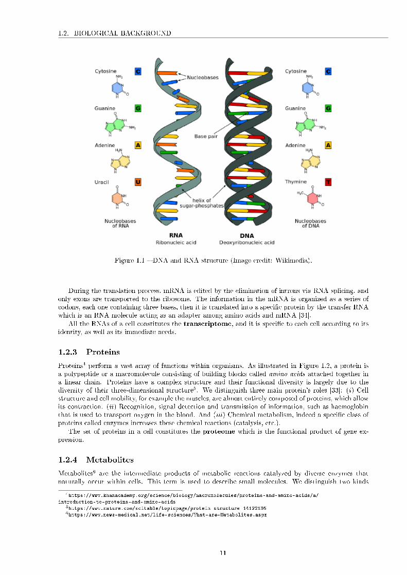
Figure 1.1 � DNA and RNA structure (Image credit: Wikimedia).
During the translation process, mRNA is edited by the elimination of introns via RNA splicing, andonly exons are transported to the ribosome. The information in the mRNA is organized as a series ofcodons, each one containing three bases, then it is translated into a speci�c protein by the transfer RNAwhich is an RNA molecule acting as an adapter among amino acids and mRNA [34].
All the RNAs of a cell constitutes the transcriptome, and it is speci�c to each cell according to itsidentity, as well as its immediate needs.
1.2.3 Proteins
Proteins4 perform a vast array of functions within organisms. As illustrated in Figure 1.2, a protein isa polypeptide or a macromolecule consisting of building blocks called amino acids attached together ina linear chain. Proteins have a complex structure and their functional diversity is largely due to thediversity of their three-dimensional structure5. We distinguish three main protein's roles [33]: (i) Cellstructure and cell mobility, for example the muscles, are almost entirely composed of proteins, which allowits contraction. (ii) Recognition, signal detection and transmission of information, such as haemoglobinthat is used to transport oxygen in the blood. And (iii) Chemical metabolism, indeed a speci�c class ofproteins called enzymes increases these chemical reactions (catalysis, etc.).
The set of proteins in a cell constitutes the proteome which is the functional product of gene ex-pression.
1.2.4 Metabolites
Metabolites6 are the intermediate products of metabolic reactions catalyzed by diverse enzymes thatnaturally occur within cells. This term is used to describe small molecules. We distinguish two kinds
4https://www.khanacademy.org/science/biology/macromolecules/proteins-and-amino-acids/a/
introduction-to-proteins-and-amino-acids5https://www.nature.com/scitable/topicpage/protein-structure-141221366https://www.news-medical.net/life-sciences/What-are-Metabolites.aspx
11

1.2. BIOLOGICAL BACKGROUND
Figure 1.2 � Protein structure (Image credit: Wikimedia).
of metabolites: (i) The primary metabolites which are synthesized by the cell because they are indis-pensable for its growth, such as amino acids, alcohols, vitamins, organic acids, nucleotides (inosine-5'-monophosphate and guanosine-5'-monophosphate) [33]. And (ii) the secondary metabolites which arecompounds produced by an organism that is not required for primary metabolic processes, although theycan have other functions. As illustrated in Figure 1.3 displays the structure of some metabolites.
The set of primary and secondary metabolites constitutes the metabolome. Unlike the genome, thetranscriptome and the proteome, the metabolome is not encoded.
We must also note that metabolites can be the reactants, products of the metabolic pathway whichis a linked series of chemical reactions occurring within a cell.
1.2.5 Gene expression
As discussed previously, the DNA stores all the genomic information required for a cell to operate. Geneexpression focuses on the study of the process by which the instructions in DNA are converted into afunctional product which is called 'the central dogma of molecular biology ' [33, 35, 36, 37]. This clari�esthe �ow of genetic information from DNA to RNA to produce a protein. The process by which theDNA instructions are converted into proteins is called gene expression, which has two main steps: (i) thetranscription and (ii) the translation [37].
In the transcription step, the information in the DNA of every cell is converted into small, portablemRNA. And during the translation step, these mRNA travel from the cell nucleus to the ribosomes wherethey are ready to make speci�c proteins.
As described in Figure 1.4, we distinguish three states of the central dogma:
• From existing DNA to make new DNA: DNA replication phase,
• From DNA to make new RNA: transcription phase,
• From RNA to make new proteins:translation phase.
The gene expression process starts with the DNA replication in which there is a production of identicalDNA helices from a single double-stranded DNA molecule in order to ensure that each new cell receivesthe correct number of chromosomes. The gene expression has transcription as a second step [36]. Here,one of the DNA double helices serves as a template for the production of the RNA. In post-transcriptional
12

1.2. BIOLOGICAL BACKGROUND
Figure 1.3 � Examples of metabolites (Image credit: the West Coast Metabolomics Center).
Figure 1.4 � The central drogma of life.
processing, a pre-mRNA is edited to contain only coding sections (exons) to form a mature mRNA script.The mRNA is then transmitted to the cytoplasm where it is matched to ribosomes for protein synthesis[33]. Finally, the tRNA attaches speci�c amino acids to the mRNA to form complete polypeptide chains:the proteins. Thus this translation phase ensures the conversion of the genetic information in DNA intoproteins.
Therefore, genome, transcriptome, proteome and metabolome are the major molecular com-plexes of cells [38, 39]. A correlation among these four large sets can be explained by the expression of thegenome de�nes a transcriptome, then a speci�c proteome determines the metabolome. In contrast, themetabolome regulates gene expression so that the cell permanently adapts its proteome to its metabolicstate. However, it should not be forgotten that the control of the metabolome is only part of one of theproteome's functions, which also realize many other roles such as the communication of the cell with itsenvironment or the structuring of the cell [33].
Merging proteomic, transcriptomic, and metabolomic information to facilitate the study of cellularbehaviour, is among the major aims of systems biology.
13

1.3. FROM MOLECULAR BIOLOGY TO SYSTEMS BIOLOGY
1.3 From molecular biology to systems biology
In the 20th century, there has been an important revolution of molecular biology. This advance is due tothe explosion of high-throughput technologies which generate huge amounts of molecular-level data. Theseso-called 'omics' (genomic, transcriptomic, proteomic and metabolomic) techniques aimed primarily atthe detection and the study of genes (total gene expression analysis [40]), RNAs (RNA-Seq [41]), proteins(mass spectrometry [42]) and metabolites (liquid chromatography [43]) in a speci�c biological sample [44].However, despite these advances, the molecular biology of the 20th century has remained fragmented andincomplete. Indeed, each laboratory focus only on a particular phenomenon concerning a cellular type ofa speci�c organ in an environment. This limitation is due to the inability of classical biological approachesto address biological systems as wholes and thus to confront their complexity. This complexity resultsfrom the heterogeneity and diversity of the components involved, the dynamic nature of the interactionsamong these components, and the non-linear nature of the behaviour resulting from these interactions.
According to Sauer et al. in [45]: 'The reductionist approach has successfully identi�ed most of thecomponents and many of the interactions but, unfortunately, o�ers no convincing concepts or methods tounderstand how system properties emerge . . . the pluralism of causes and e�ects in biological networks isbetter addressed by observing, through quantitative measures, multiple components simultaneously and byrigorous data integration with mathematical models'.
To �ll these gaps, the area of systems biology was introduced to complete classical biological ap-proaches. Systems biology is an approach that addresses the complexity of biological systems and theirdynamic behaviour at all relevant organizational levels (from molecules, cells and organs to organisms).It combines reducing and integrative methods to emphasise both the components of the system and theinteractions among them which generate emergence phenomena at higher organizational levels.
In contrast to classical biology, this �eld is based on the understanding that the whole is greater thanthe sum of the parts7. It approaches the complexity of biological systems with the integration of manyscienti�c disciplines such: biology, computer science, engineering, bioinformatics, physics and others, topredict how these systems change over time and under diverse conditions.
It is now clear in the minds of all biologists that understanding cellular behaviour requires analysisof its dynamic interactions (its evolution), its multi-variate data (measurements of millions of moleculesand multiple parameters) and its multi-level data (from genome to metabolome).
1.4 Complex biomolecular networks
As discussed in the previous section, with the rapid accumulation of omics-data from high-throughputtechnologies, the study of biomolecular networks has become one of the keys focuses in systems biol-ogy. Indeed, high-throughput technologies pave the way for the reconstructions of di�erent biomolecularnetworks according to molecular-level de�ned by omics data. Figure 1.5 depicts the di�erent types ofbiological networks according to molecular components using high-throughput omics technologies. Inthis section, we review these di�erent types of molecular networks and de�ne the complex biomolecularnetwork.
Therefore, depending on the type of its cellular elements and their interactions, we can distinguish thethree basic types of networks, the Gene Regulatory networks (GRNs), the Protein-Protein Interactionnetworks (PPINs), and the Metabolic networks (MNs).
• The Gene Regulatory networks (GRNs) describe the interactions among approximately 21,000 genes(DNAs and RNAs). They are represented as directed graphs where the nodes represent genes andedges model the type of regulation (activation or inhibition) if one gene regulates the transcriptionof the other gene [46].
• The Protein-Protein-Interaction networks (PPINs) model the interactions among proteins withinan organism (about 80,000 proteins in the human organism). These networks are represented asundirected graphs where the nodes are the proteins and the undirected edges model the connectionbetween them. These types of interactions depend on the physical or biochemical interaction thatexists between the pair of proteins [47]. This network mainly contains details on how proteinsperform together to ensure the biological processes.
7https://www.systemsbiology.org/about/what-is-systems-biology/
14

1.4. COMPLEX BIOMOLECULAR NETWORKS
Figure 1.5 � Types of biological networks according to molecular components using high-throughputomics technologies.
• The metabolic process consists of a series of chemical reactions that begins with a particular metabo-lite called 'substrate' and converts it into some other metabolites called 'products' [48]. Thus, theMetabolic networks (MNs) describe the biochemical reactions among approximately 42,000 metabo-lites. They are represented as directed graphs whose nodes are the metabolites and the edges repre-sent the type of the biochemical reaction which transforms the substrates into products by the helpof enzymes. They are labelled by the stoichiometric coe�cient of the metabolites in the reaction.
Figure 1.6 � Multi-level modelling of a biomolecular network from a real cell.
As discussed above, the cell is a complex system consisting of thousands of diverse molecular entities(genes, proteins and metabolites) which interact with each other physically, functionally and logically cre-ating a biomolecular network [6, 14]. Indeed, omics technologies describe the cell networks and processesthrough the study of cellular entities. These technologies operate at various levels such as in genomics (thequalitative study of genes), in proteomics (the quantitative study of proteins) and in metabolomics (thequantitative study of metabolites) [49, 50]. Thus, the complexity of this complex biomolecular network
15

1.5. TRANSITTABILITY OF COMPLEX BIOMOLECULAR NETWORKS
appears by its decomposition into the three levels presented above: the genome, transcriptome, proteomeand metabolome which are the major molecular complexes composing the cell [38, 39]. As illustrated inFigure 1.6, complex biomolecular networks typically include gene regulatory networks, protein-proteininteraction networks and metabolic networks. It consists of di�erent types of nodes, denoting cellularentities, and various nature of edges, representing interactions among cellular components.
This complex network facilitates the understanding of biological mechanisms of a cell and its transit-tability.
1.5 Transittability of complex biomolecular networks
Figure 1.7 � The transittability of the P53-mediated cell damage response network: colour changes in thenodes indicate changes in the concentration of the associated molecules.
Cells do not live in stable conditions, but in environments that vary over time [9]. In fact, theyare always subjected to intra and extra-cellular stimuli, such as changes in their physical and chemicalproperties or in their environment. In order to survive, the cell reacts more or less rapidly by adaptingits behaviour in accordance with the new features of its environment. As discussed in the previoussection, biomolecular components interact with each other to form so-called biomolecular networks, whichdetermine the cellular behaviours of living organisms. Indeed, controlling the cellular behaviours byregulating some biomolecular components in the network is one of the most outstanding problems insystems biology.
Recently, some authors have started to address the dynamic aspects of biological systems, and haveintroduced concepts such as the 'controllability' [28, 51] of a network, where the ability to steer a complexdirected network from any initial state toward any other desired state is measured by the minimum numberof required driver nodes (nodes with the ability to steer the entire network). It has been shown that inorder to achieve complete controllability, the minimum number of driver nodes is 80% of the nodesin a regulatory biomolecular network. This result led other groups to develop a theoretic frameworkfor studying transitions between two speci�c states of directed complex networks, a concept they call
16

1.6. SUMMARY
'transittability' [6]. In general, this concept expresses the idea of steering the complex biomolecularnetwork from an unexpected state to a desired state. The theorems were developed with continuous-timelinear time-invariant systems (a theory investigating the response of a linear and time-invariant systemto an arbitrary input signal) and applied to 4 di�erent biological systems consisting of up to 17 moleculesand 40 interactions. Figure 1.7 shows an example of a biological system. At each stage of this network,the blue-�lled node indicates that the level of this node concentration at that state, a blue-�lled nodemeans high level and an empty node means low level. For more details about the components of theP53-mediated cell damage response network, please refer to the TP53 website at http://p53.fr/ whichcontains extensive information on various aspects on p53 and also links to other p53 sites. Moreover, thisexample is described in detail in [6].
With the idea of making the biomolecular network evolve, our research works aim to design and developa platform that provides an optimal set of external stimuli to be applied during a predetermined timeinterval to steer the biomolecular network from its current state to a desired state. Our original approachis based on the cooperation of semantic technologies [52], combinatorial optimization and simulation.
1.6 Summary
In this chapter, we presented the biological environment we are working in by de�ning its main conceptssuch as DNA, ARN, proteins, metabolites and gene expression. Then we give a brief history of biologyarea describing its revolution from the classical molecular biology to the appearance of systems biology.We discussed also how omics technologies operate at various levels (genomics, proteomics, metabolomics)creating complex biomolecular networks. Finally, we discussed some concepts which are introducedto study the dynamic behaviour of complex biomolecular networks, such as the 'controllability' and'transittability', some of which have inspired the work presented in this thesis.
In the next chapters, we will present the state-of-the-art of the di�erent disciplines covered by thisthesis.
17

1.6. SUMMARY
18

Chapter 2
Modelling in systems biology
Contents2.1 Introduction . . . . . . . . . . . . . . . . . . . . . . . . . . . . . . . . . . . . . 20
2.2 Major properties and dimensions of modelling . . . . . . . . . . . . . . . . . 20
2.2.1 Discrete vs Continuous vs Hybrid models . . . . . . . . . . . . . . . . . . . . . 20
2.2.2 Quantitative vs Qualitative models . . . . . . . . . . . . . . . . . . . . . . . . . 21
2.3 Overview of the existing mathematical models in systems biology . . . . . 21
2.3.1 Boolean models . . . . . . . . . . . . . . . . . . . . . . . . . . . . . . . . . . . . 21
2.3.2 Logical models . . . . . . . . . . . . . . . . . . . . . . . . . . . . . . . . . . . . 21
2.3.3 Petri nets models . . . . . . . . . . . . . . . . . . . . . . . . . . . . . . . . . . . 22
2.3.4 Bayesian network models . . . . . . . . . . . . . . . . . . . . . . . . . . . . . . 22
2.3.5 Graphical Gaussian models . . . . . . . . . . . . . . . . . . . . . . . . . . . . . 22
2.3.6 Di�erential equation models . . . . . . . . . . . . . . . . . . . . . . . . . . . . . 23
2.3.7 Cellular automata models . . . . . . . . . . . . . . . . . . . . . . . . . . . . . . 23
2.3.8 Agent-based models . . . . . . . . . . . . . . . . . . . . . . . . . . . . . . . . . 23
2.4 Comparison among these modelling formalisms . . . . . . . . . . . . . . . . 24
2.5 Thesis contribution in this �eld . . . . . . . . . . . . . . . . . . . . . . . . . . 26
2.6 Summary . . . . . . . . . . . . . . . . . . . . . . . . . . . . . . . . . . . . . . . 26
19

2.1. INTRODUCTION
2.1 Introduction
Numerous formalisms have been proposed in the literature for describing and studying biological networks.Indeed, modelling these complex systems is the �rst step towards understanding, designing, simulatingand controlling the behaviour of these biological networks [53]. Therefore we can use di�erent kindsof models: discrete, continuous or hybrid models for the same biological network. This classi�cation isdone according to the nature of the mathematical formalisms used (Boolean, logic, di�erential equations,etc.) [54]. Thus, each model focuses on a speci�c problem and treats a well-de�ned level of intracellularabstraction.
This chapter aims to classify and detail these mathematical tools for modelling biological networks.We �rstly introduce a classi�cation of modelling tools based on their major properties and then highlightsome of the most popular and important mathematical models in systems biology. Finally, we provide acomparison among these modelling formalisms and discuss their main characteristics.
2.2 Major properties and dimensions of modelling
With the explosion of high-throughput technologies which generated huge amounts of molecular-level omicdata, it becomes necessary to provide models that can be used to understand and formalize knowledgeabout them. Therefore several mathematical models have been proposed in the literature. These modelsare very varied from the point of view of abstraction levels (from the gene level to the metabolic levelthrough proteins), details of analysis (discrete, continuous), etc. A number of bibliographic reviewsfocused on these modelling tools. Most of them classify these models according to di�erent criteria. Inthe following section, we will focus on these categories and detail some of the most popular models.
2.2.1 Discrete vs Continuous vs Hybrid models
2.2.1.1 Discrete models
These methods consider a molecular component as an object that can steer from a state to another andrepresent the biological interactions among these entities as Boolean functions [55]. Discrete models sim-plify the calculation and o�er the possibility of realizing formal checks. However, despite their simplicityto model and simulate speci�c biological questions, they are too complex when the user focuses on animportant number of states. Moreover, modelling a molecular component by a Boolean value do not takeinto account the reality because it can not have intermediate states [56].
2.2.1.2 Continuous models
In order to understand in detail the functioning of a biological system (especially from a temporal pointof view), this approach focuses on its continuous evolution. The variables represent the concentrations ofmolecular components comprising the system, and the global evolution is guided by a system of di�erentialequations. This approach can be close to the real-life but is di�cult to implement when the size of thesystem is high. This complexity is due to the non-linear character of the di�erential equations. To addressthis limits, an intermediate approach called hybrid model was proposed.
2.2.1.3 Hybrid models
They are dynamical models that combine the advantages of both discrete and continuous models. Theprinciple is to mix between the classic di�erential equations representing the evolution of chemical con-centrations, with cellular automata or agent-based models representing the individual behaviour of somemolecular components of interest. Thus, a hybrid model corresponds to any interaction or coupling be-tween two or more models that are not based on the same formalism [57]. More details about hybridmodelling in biology are presented in a review Hybrid Modelling in Biology: a Classi�cation Review [57]written by Stéphanou and Volpert.
20

2.3. OVERVIEW OF THE EXISTING MATHEMATICAL MODELS IN SYSTEMS BIOLOGY
2.2.2 Quantitative vs Qualitative models
2.2.2.1 Quantitative models:
They are usually represented as a set of di�erential equations given that they are a suitable approach formodelling real systems. These models require all the parameters to be de�ned, but given the large sizeof biological systems, it is not possible to list all of them, moreover, their values are not yet known.
2.2.2.2 Qualitative models:
Unlike quantitative models, these models provide general descriptions of biological systems because theyrequire few or no parameters. These models are usually representing as discrete or hybrid models.
A detailed comparison study between quantitative and qualitative models can be found in [58].
2.3 Overview of the existing mathematical models in systems bi-
ology
Biological networks are extremely complex. To understand their operation, we not only need to identifytheir molecular components (genes, proteins and metabolites) and their interactions but also we need toknow how their dynamics evolve over time [59].
This section highlights some of the most popular and important modelling tools.
2.3.1 Boolean models
Boolean network models were initially proposed as a special case of discrete dynamic models. A Booleannetwork model consists of a set of nodes whose state is binary (0 or 1 ) and is determined by othernodes in the network through Boolean functions. These Boolean functions are expressed together withthe logical operators: AND, OR, and NOT. In terms of complexity, Boolean networks lie between staticnetwork models and continuous dynamic models, making them attractable and powerful approaches tomodel large-level biological systems. Boolean models can be used to describe the qualitative temporalbehaviour of the system and to understand how perturbations change its behaviours. They also providea coherent network representation.
This Boolean model has been applied to the modelling of several genetic regulation networks of diverseorganisms such as: the di�erentiation of �oral organs in Arabidopsis thaliana plants [60], the embryonicdevelopment of Drosophila [61], the mammalian cerebral cortex [62], the process of apoptosis (cell death)[63], and signalling networks in a variety of biological systems such: the ABA Signal Transduction network[64], the Embryonic stem cells (ES cells) [65].
2.3.2 Logical models
The logical approach was initially developed by René Thomas and his collaborators [66], then it wasintroduced in biology by Kau�man [18, 56]. This model represents a compromise between the staticmodel (structural analysis) and di�erential equations in terms of complexity and precision [67]. In alogical graph, the nodes represent genes which are associated with discrete levels of expression, and edgesrepresent the interactions among genes. Each interaction is associated with an expression level thresholdfrom which the regulator (starting node of the interaction) has an e�ect on the target gene. For eachgene, a discrete logical function indicates to which qualitative level the gene tends when he is submittedto a given combination of interactions. In their simplest form, logic models associate to each molecularcomponent one of this two discrete states: ON or OFF. Therefore, logic models with only two binarystates are generally considered as Boolean models.
Logic models have been applied to the modelling of several signal transduction pathways involved indiverse processes such as: proliferation [68], cell cycle regulation [69], apoptosis [70], or di�erentiation[71]. A detailed survey of logic models can be found in [72].
21

2.3. OVERVIEW OF THE EXISTING MATHEMATICAL MODELS IN SYSTEMS BIOLOGY
2.3.3 Petri nets models
Petri net is a graphical and mathematical approach for modelling systems in which the notion of eventsand evolution is important. Initially, this model was developed by Petri in 1962 [73] to represent discrete-event systems. Originally, only systems that changed discreetly could be represented with Petri networks.Then, many extensions were produced (Wim Bos list the main extensions in [74]). Some of them arereally dedicated to biological system modelling, such as the hybrid Petri net networks which are usedto model the evolution of systems in which some variables evolve discreetly, others continuously, andwhose rates of change depending on the system's variables. In general, a Petri net is a directed, weightedbipartite graph consisting of two types of nodes: places and transitions. In this network, circles representthe places and boxes represent the transitions. We usually consider a token to be a unit of weight of amolecule. A place-transition or transition-place connection is made by a weighted edge representing howmuch of the input places (reactants) are required to produce tokens for the output places (products) in areaction. A transition can only �re when it is enabled, meaning that each of its input places has at leastone token in the current marking. More formally, a Petri network consists of �ve elements:
• P = {p1, p2, . . . , pm} a set of places,
• T = {t1, t2, . . . , tn} a set of transitions,
• F ⊆ (P ∗ T ) ∪ (T ∗ P ) a set of edges,
• W : F → {1, 2, 3, . . .} a weight function,
• M0 : P → {0, 1, 2, 3, . . .} the initial marking.
Petri net was mainly used to model signalling pathway networks [75]. This signaling Petri net aims topredict signal �ow through a cell-speci�c network in experimental conditions [75]. Each place is devotedto a signaling protein, and each transition is associated with a phosphorylation interaction.
A number of research studies have been focused on Petri net to model biological systems such asfor modelling and validation of the sucrose breakdown pathway in the potato tuber [76], the enzymaticreaction chains [77], and the biochemical reaction systems [78]. More details on approaches using Petrinet for modelling biological systems can be found in dedicated survey [79, 80, 81].
2.3.4 Bayesian network models
The Bayesian models were initially introduced into biology issues in order to infer regulatory networksfrom DNA chips by Friedman et al. in [82]. Then, Microsoft's research contributed to the developmentof approaches based on Bayesian models [83, 84]. In a Bayesian model, the variables can be discrete orcontinuous. Bayesian models are static in nature, but they are easily extensible to dynamic modellingproblems [85].
This graphical formalism de�nes and simpli�es a joint law of probabilities of a model. It is, therefore, agraphical and probabilistic model. The variables have a probability distribution conditioned by the stateof other variables in the model. These variables represented by nodes are associated with conditionalprobability distributions. The edges indicate a statistical dependence between two variables [86]. Bayesiannetwork model consists of three major steps: (i) the structure must be proposed, (ii) the parameters orprobabilities associated with edges and nodes must be set, and (iii) the �nal network must be evaluated.
Bayesian networks have been applied for inferring the structure of many biological networks from ex-perimental data. Among these applications, we can cite the Characterizing Loss Of Cell Cycle Synchrony(CLOCCS) [87], the comparison of Acute Lymphoblastic Leukemia (ALL) [88].
2.3.5 Graphical Gaussian models
Graphical Gaussian models also called covariance selection or concentration graph models, have beenused to model gene association networks. The main objective of Graphical Gaussian models is to usepartial correlations as a measure of independence of any two genes. This model relies on assessingthe conditional dependencies among genes in terms of partial correlation coe�cients among the geneexpressions and results are displayed in an undirected network [89]. A detailed introduction to GraphicalGaussian models can be found in [90] and [91].
22

2.3. OVERVIEW OF THE EXISTING MATHEMATICAL MODELS IN SYSTEMS BIOLOGY
Graphical Gaussian models have been applied for inferring the genetic network of many biologicalsystems such as the genetic network of S. cerevisiae [92], the Arabidopsis thaliana transcriptome [93], theisoprenoid gene network in Arabidopsis thaliana [94].
2.3.6 Di�erential equation models
Among dynamic modelling methods, the most commonly used in biology is the di�erential description.Concentrations or activities of molecular components are usually represented by positive real quantitiescalled also variables which can vary continuously over time. The variation of these quantities is formalizedby writing a system of coupled di�erential equations. Thus, molecular components and their interactionsconstitute a system of ordinary di�erential equations. In most biological systems, the interactions con-sidered are non-linear which leads to di�erential models that are almost impossible to solve and analyse.Consequently, this model requires the use of 'numerical simulations'. Starting from initial constraints andconditions, this model tries to have a solution similar to the exact solution by calculating the values of theconcentrations of molecular components involved over time, using small time intervals. Moreover, thisapproach requires to de�ne the values for all parameters. Since these values are not always establishedexperimentally, simulations are carried out with very approximate or arbitrary values. Therefore, it isdi�cult to predict the dynamic behaviour of the biological system. Thus, this method can be used tomodel small systems where it is possible to know in advance the exact values of their parameters, butfor more complex biological models, it is di�cult to specify all the corresponding dynamic properties andassociated conditions.
During the last decades, several kinds of researches have been proposed to describe the regulation ofgene expression using a di�erential equation model. Among them, we can cite [95, 96, 97, 98, 99, 100].Diláo et al. [101] developed the 'GeneticNetworks' which is a software tool, for modelling genetic networksusing linear di�erential equations. Other authors have proposed and simulated di�erential models formolecular networks, for example in the gene expression regulation in bacteria [102], cell-cycle control [103],Circadian rhythms [104], speci�c gene expression pro�les during embryonic development [105, 106, 107]and response of Escherichia coli cells to carbon deprivation [108]. Moreover, di�erential equations modelshave been used to model metabolic networks, for example for analysing the central metabolism of anenvironmental bacterium: the Methylobacterium extorquens in [109] or in Corynebacterium glutamicum[110]. Di�erential equation models are also applied to protein-protein interaction networks (only fromthe perspective of studying signal transduction networks) as studying feedback e�ects on signal dynamicsin a Mitogen-Activated Protein Kinase (MAPK) [111], controlling signal transduction cycles [112], andunderstanding the CovR/S signal transduction system in [113].
2.3.7 Cellular automata models
Cellular Automata model is a discrete dynamical formalism. Within this model the notions of space,time, and states of the system are discrete. Each point in the spatial network is called a cell which mayhave any one of the �nite numbers of states. The states of the cells in the network are updated accordingto a local rule. Consequently, the state of a cell at a given time t depends only on its state at time t− 1and the states of its neighbours at time t−1, and all the cells on the network are updated synchronously.Using cellular automata it is possible to model diverse systems. The �rst works on cellular automatawere made by Von-Neumann in [114]. Subsequently, this model was detailed by Stephen Wolfram in the1980s [115].
Application of cellular automata models can be seen in the modelling of the immune system [116], thedevelopment of an arti�cial brain [117], the enzymatic reaction [118] and some other biological systems[119].
2.3.8 Agent-based models
Agent-based model is a rule-based, discrete-event and discrete-time computational modelling method-ology that employs computational objects focusing on the rules and interactions among the individualcomponents (agents) of the system [120, 121, 122].
An agent is an interactive computer system situated in an environment and able to autonomous actionin this environment in order to meet its design objectives. A multi-agent system consists of a set of agents
23

2.4. COMPARISON AMONG THESE MODELLING FORMALISMS
interacting in a dynamic environment as de�ned by Michael Wooldridge in [123].
Application of agent-based models can be seen in the modelling of the control pathways a�ectingthe transcription factor nuclear factor kappa B (NF-kB) [124], the behaviour of the toll-like receptor 4(TLR-4) signalling pathway [125] and the Pseudomonas aeruginosa Bio�lm Formation [126].
2.4 Comparison among these modelling formalisms
As detailed above, biological systems and in particular intracellular components have been modelledby diverse modelling approaches. This diversity is essentially due to the complexity and heterogeneityof the molecular components and their interactions [54]. After analysing each modelling approach, weshould note that each model has its own bene�ts and drawbacks, and can be used according to the user'sobjective.
Indeed, there is no perfect approach to model a complex biomolecular network considering all its levelsand their molecular components. Moreover, we note that there is no agreement on the classi�cation ofthese models because we cannot compare them on the basis of a particular criterion. The same modelcan be used in di�erent ways with di�erent interpretations of biology. But, we note that these modelsdi�er in many other criteria including how to interpret biological facts. In order to highlight theirproperties and their utility, we compare them according to various criteria. The classi�cation proposedhere aims to illustrate the major characteristics of each approach for modelling biological systems. Table2.1 summarises the main features of these models.
For example, Boolean models have the capacity to simplify the dynamics of gene networks whichenable an e�cient analysis of large-scale networks. However, it ignores the intermediate states of geneexpression and it can update the gene in an asynchronous way which may miss many important dynamicbehaviours.
The power of Petri net models is their capacity to provide an intuitive representation of a biologicalsystem due to their graph-based structure which is suitable for analysing the global behaviour of thesystem. However, the graphical representation becomes too complex for analysis when the biologicalnetwork is large because it requires to de�ne a lot of transition rules.
Bayesian networks provide a graphical formalism de�ning a joint law of probabilities of a modelwhich is easily extensible. However, they are computationally expensive because it needs to analyseall potential network topologies corresponding to all possible sets of directed acyclic graphs linking themolecular components. This causes a combinatorial explosion of the number of possible structures andparameters creating an NP problem.
Graphical Gaussian models provide a powerful model to represent statistical dependencies amongrandom variables. However, they su�er from poor scalability and interpretability.
Di�erential equation models have the capacity to model and analyse the dynamics of the system. Thismodel provides a result similar to the exact and real solution. However, the power of this model can onlybe applied to a small-scale system. In fact, despite the evolution of high-throughput technologies, thereis always a lack of data. Moreover, if the network scale is large, parameter estimation will generate a highcomputational cost. Indeed, the simulation of large-scale networks using di�erential equations cannotbe performed because of the complexity of the problem and the high number of network components.Also, the quantitative parameters of biological systems cannot be experimentally measured. This leadsto creating more di�culties in setting the inial conditions of the network simulation. We note thatdi�erential equation models are more precise and speci�c about a system, but require a large e�ort inmodel construction and a complete set of quantitative data.
Agent-based models can be constructed in the lack of complete knowledge about the system using sim-ple rules. Also, these models easily incorporate space because they have their origins in two-dimensionalcellular automata. Agent-based models incorporate stochastic aspects. However, they do not allow to�nd patterns in an existing dataset. Moreover, they require a lot of interactions among each agent andthey need frequent communication.
Table 2.1 classi�es these modelling methods according to their properties.
24

2.4. COMPARISON AMONG THESE MODELLING FORMALISMS
Table2.1�Tableof
themainapproaches
appliedto
modellin
gbiological
networks.
Model
Di�erential
equa-
tion
Boolean,
Logic
models
Petrinetsnetwork
Graphical
Gaus-
sian
Bayesiannetwork
Agentbasedmodel
Cellularautomata
Analysis
type
quantitative
qualitative
qualitative
quantitative
qualitative
qualitative
qualitative
Category
continuous
discrete,stochastic
discrete,
continu-
ous
stochastic,contin-
uous
discrete,
continu-
ous
discrete,
continu-
ous
discrete,
continu-
ous
Advantages
quantitative
dy-
namics,
suitable
for
modelling
small-scale
net-
works,
analytical
models
simplify
the
dy-
namics
of
gene
network,
e�cient
analysis
of
large
network
representation
of
the
concentration
�ow
,intuitive
and
hierarchically
modelling
computational
ef-
�ciency,represent
rich
statisticalde-
pendencies
among
random
variables
intuitiverepresen-
tationofbiochem
i-calnetworksdueto
their
graph-based
structure
representation
of
cells
hav-
ing
aspeci�c
behaviour,
incor-
porate
stochastic
aspects
space
representa-
tion,easy
toun-
derstandresults
Limits
need
for
quanti-
tative
data,
high
computational
cost
ignore
the
inter-
mediate
states
of
gene
expression,
miss
many
im-
portant
dynamic
behaviours
number
of
un-
bounded
tokensin
basic
semantics,
inabilityto
testfor
exactly
aspeci�c
marking
inan
unbounded
place
andto
takeaction
ontheoutcomeof
thetest
poor
scalability
and
interpretabil-
ity,
di�
cult
toidentify
high-level
interactions
be-
tween
functional
variables
high
computa-
tional
cost,
an
NP-Complete
problem
lack
ofanalytical
methods,
requires
alot
of
interac-
tionsamong
each
agent
lack
ofanalytical
methods
25

2.5. THESIS CONTRIBUTION IN THIS FIELD
2.5 Thesis contribution in this �eld
Several studies have been conducted to model, analyse and understand the behaviour and processesof cells. However, most of them do not examine the interactions among all the intervening moleculestypes and do not consider the di�erent abstraction level within the cell. As a result, these modellingapproaches are impractical to understand the transittability of complex biomolecular networks. Therefore,to accomplish this task, we must take into account the analysis of the structure and dynamics of the wholecell rather than just focusing on isolated parts [24, 25, 26, 27].
With this idea in mind, we think that a formal logic-based formalism is needed for modelling and un-derstanding complex biomolecular networks as a whole considering its structure, function and behaviour.Indeed, we aim to design and develop a logic formalism for biologist that allows (i) the formal expressionof various types of biological knowledge, (ii) the translation of this knowledge into logical notions foranalysis, simulation and optimization, (iii) the integration of the di�erent levels of intracellular abstrac-tion (genomic, proteomic and metabolic). Therefore, this model will be considered as a well-organizedknowledge base that contains all the available information for modelling a biological network in a logic,clear and consistent manner.
It is important to note that this logic-based model can be considered as a logical model. Logical modelsrepresent one of the youngest approaches to model and formalize the multi-level aspect of biomolecularnetworks underlying their di�erent level properties. Indeed, this model is capable of modelling thebiomolecular network processes and functions on di�erent temporal and spatial levels in an explicit way.Moreover, this multi-level model can be a good framework for the integration of additional computationalmodule, in our case it serves to integrate the logic modelling with the semantic modelling module, thesimulation module and the optimization module. All of these modules are based and joined togetherusing this logic-based model. Using this type of models, we can also integrate discrete with continuousmodelling, thereby opening the possibility to simulate modules that can be best represented with discretevalues and modules best described using continuous equations. Furthermore, this model o�ers a higherexpressive power due to its formal language. Indeed, in these logical models, there is a class of wellde�ned mathematical structure in which the domain knowledge (all the elements required for modellingbiomolecular networks) is interpreted.
2.6 Summary
In this chapter, we focused only on some popular mathematical modelling tools. Many literature reviewsdetailed these modelling approaches and are available in [26, 127, 128]. In fact, di�erent modellingapproaches are used in systems biology and we cannot say that a model is better than other. As detailedabove, some models are too small systems, others to large systems, and some of them are qualitative,others are quantitative. Each of these models focuses on a speci�c problem and treats a well-de�ned levelof intracellular abstraction. These models can also be applied to the same biological network to studydi�erent problems with di�erent point of views. However, all these models are not adequate and do notallow to understand the transittability of complex biomolecular networks. In fact, they are more speci�cand oriented to a particular problem in systems biology. Therefore, with the goal of understanding andanalysing the transittability of biomolecular networks, we need to implement a more speci�c model whichcan provide all the elements required for studying this problem. That is why we hope to contribute to thisdiscipline by proposing a logical-based approach for modelling the dynamic behaviour of biomolecularnetworks. This formalism is based on the three levels of analysis de�ned by the systems theory: structural,functional and behavioural modelling. Indeed, it aims at describing and analysing all the properties andmechanisms of complex biomolecular networks. This logic-based modelling will form the basic elementfor modelling and understanding the transittability of these complex networks.
Despite existing mathematical modelling tools for formalizing biological networks, there are also se-mantic technologies which are useful to provide a powerful integration and management of availablebiological data and knowledge, thus making them more understandable to biologists, enabling an e�-cient analysis of biological networks and reasoning. The next chapter is devoted to exploring the role ofsemantic technologies, especially ontologies in systems biology.
26

Chapter 3
Ontologies in systems biology
Contents3.1 Introduction . . . . . . . . . . . . . . . . . . . . . . . . . . . . . . . . . . . . . 28
3.2 Concept of Ontology . . . . . . . . . . . . . . . . . . . . . . . . . . . . . . . . 28
3.3 Ontology components . . . . . . . . . . . . . . . . . . . . . . . . . . . . . . . . 28
3.4 Typologies of ontologies . . . . . . . . . . . . . . . . . . . . . . . . . . . . . . 29
3.4.1 According to the object of generality . . . . . . . . . . . . . . . . . . . . . . . . 29
3.4.2 According to the level of detail . . . . . . . . . . . . . . . . . . . . . . . . . . . 29
3.4.3 According to the level of formality . . . . . . . . . . . . . . . . . . . . . . . . . 30
3.5 Ontology building: methodologies, formalisms, languages and tools . . . . 30
3.5.1 Ontology engineering methodologies . . . . . . . . . . . . . . . . . . . . . . . . 30
3.5.2 Types of formalisms . . . . . . . . . . . . . . . . . . . . . . . . . . . . . . . . . 31
3.5.3 Languages . . . . . . . . . . . . . . . . . . . . . . . . . . . . . . . . . . . . . . . 32
3.5.4 Editing tools . . . . . . . . . . . . . . . . . . . . . . . . . . . . . . . . . . . . . 34
3.6 Ontology reasoning . . . . . . . . . . . . . . . . . . . . . . . . . . . . . . . . . 35
3.6.1 Semantic Web Rule Language . . . . . . . . . . . . . . . . . . . . . . . . . . . . 35
3.6.2 SWRL sytax . . . . . . . . . . . . . . . . . . . . . . . . . . . . . . . . . . . . . 35
3.6.3 Reasoning systems for description logic . . . . . . . . . . . . . . . . . . . . . . 35
3.7 Overview of existing ontology applications in systems biology . . . . . . . 35
3.8 Comparison among these bio-ontologies . . . . . . . . . . . . . . . . . . . . . 36
3.9 Thesis contribution in this �eld . . . . . . . . . . . . . . . . . . . . . . . . . . 36
3.10 Summary . . . . . . . . . . . . . . . . . . . . . . . . . . . . . . . . . . . . . . . 36
27

3.1. INTRODUCTION
3.1 Introduction
Modelling knowledge requires semantic structures and representation formalisms that translate the com-plexity of human thought and describe characteristics of the real word. Actually, it is the �eld of semantictechnologies and more particularly ontologies that address these issues. An ontology is considered as acognitive artefact allowing the conceptualization and shared exploitation of knowledge. It consists of avocabulary of the �eld in which the meaning of the terms and the relationships between the di�erentnotions are speci�ed. Beyond its descriptive ability, ontologies provide reasoning capabilities.
In this chapter, we present a complete state-of-the-art on ontologies. First, we give some backgroundinformation about ontology by presenting its di�erent de�nitions, components and typologies. Next, wedescribe the methodologies, formalisms, languages and editor tools of ontology construction. We thende�ne the di�erent languages and software for ontology reasoning. Moreover, we review the major appli-cations of ontologies in systems biology through a comparison study. Finally, we discuss the contributionof our thesis to both ontology and systems biology �eld.
3.2 Concept of Ontology
An ontology has two di�erent de�nitions depending on the �eld of interest, philosophy or computerscience:
In philosophy In philosophy, the term ontology 'is the philosophical study of the nature of being,becoming, existence, or reality, as well as the basic categories of being and their relations' 1.
In computer science In the �eld of Arti�cial Intelligence (AI) the most cited de�nition of ontology isthe de�nition proposed by Gruber [129]: 'An ontology is an explicit speci�cation of a conceptualization'.Other de�nitions of ontology for ontological engineering have been proposed and are sometimes improve-ment of already proposed de�nitions or are complementary to them. For example, Studer et al. [130]de�nes an ontology as 'a formal, explicit speci�cation of shared conceptualization'. Moreover, Pierra etal. in [131] de�ne an ontology as 'a collection of explicit, formal and consensual descriptions of all theconcepts of a domain in the context where these concepts have a precise meaning, without any restrictionor rule corresponding to a particular use'.
These proposed de�nitions gave emphasis to the notions of speci�cation and conceptualization. Theconcept of speci�cation is a formal description of how an object should be de�ned to satisfy a speci�ccriterion. Therefore, a speci�cation must be explicit because all the concepts of an ontology must beclearly de�ned. The second concept of conceptualization can be de�ned as an intentional semanticstructure that encodes implicit knowledge constraining the structure of a piece of a domain. It is usuallya logical theory that conceptualization explicitly in some language.
The following section presents the basic components of an ontology.
3.3 Ontology components
Ontologies represent the semantics of a domain's concepts in terms of classes and properties. A class alsocalled concept regroups and abstracts the domain objects having common characteristics. A propertycalled also attribute characterizes the objects of the domain by one or more values. The property can bede�ned on a domain indicating the class of objects it describes and associated with a codomain indicatingthe type of data in which it can take its values. Classes have an extension consisting of a set of instancescalled also individuals that indicate objects in the domain. An instance belongs to one or more classesand a set of property values.
Pierra et al. [131] de�nes formally an ontology by this quadruplet:
O =< C,P, Sub,Applic >
where:1https://www.merriam-webster.com/dictionary/ontology
28

3.4. TYPOLOGIES OF ONTOLOGIES
• C: represents all the classes used to describe the concepts of a given domain,
• P : represents the set of properties used to describe the instances of all the classes C,
• Sub: C → 2C is the subsumption relation which, for each class ci of the ontology, associates itsdirect subsumed classes. These classes check the property ∀c1, c2 ∈ C, c1 subsume c2 if and only if∀x ∈ c2, x ∈ c1. Sub de�nes a partial order on C and 2C denotes the power set of C,
• Applic: C → 2P associates to each ontology class the properties that are applicable for each instanceof this class.
3.4 Typologies of ontologies
Ontologies can be classi�ed according to several domains [132],[133], [134] depending on:
• the object of generality,
• the level of detail,
• the level of completeness,
• the level of representation formalism.
Each domain contains di�erent kinds of ontologies.
3.4.1 According to the object of generality
The ontology types are classi�ed into four groups according to the level of generality used in the descriptionof a domain [135].
• Top-level ontologies: These ontologies aim to de�ne the largest possible knowledge because theycontain general concepts. They are reusable among di�erent domains and reduce the ambiguityof the basis of the ontology. In these ontologies, it is rare to �nd individuals because they aimonly to propose a hierarchy of knowledge. An example of this type of ontologies in biology is theGENIA ontology [136] which propose a general description of the basic ontological entities in thelife sciences domain.
• Domain ontologies: They are a speci�cation of a high-level ontology. These ontologies specify par-ticular domains and are linked to high-level ontologies by one or more high-level ontology concepts.
• Task ontologies: They are used to describe concepts for solving speci�c activity problems. Theycontain terms and properties that describe problem solutions. These ontologies are independent ofthe domain.
• Application ontologies: A more precise level is speci�ed in the application ontologies. They describeprecisely the speci�c activities of an application domain. It is possible to consider these ontologiesas an association between task and domain ontologies.
3.4.2 According to the level of detail
According to the level of detail and the precision of the ontology, we distinguish two kinds of ontologies[137]:
• Large granularity : This type consists of high-level ontologies having a broad granularity becausethe concepts they contain will be re�ned later in other domain or application ontologies.
• Fine granularity : In contrast to the previous type, these ontologies are very detailed and have aricher vocabulary providing a detailed description of the relevant concepts of a domain or task.
29

3.5. ONTOLOGY BUILDING: METHODOLOGIES, FORMALISMS, LANGUAGES AND TOOLS
3.4.3 According to the level of formality
According to the used language or formalisms of representation, we distinguish four kinds of ontologies[138]:
• Informal ontologies: they are expressed in natural language and are easily understandable by theusers.
• Semi-informal ontologies: they are expressed in a more structured and limited.langage.
• Semi-formal ontologies: they are expressed in an arti�cial language.
• Formal ontologies: they are expressed in an arti�cial language with a formal semantics that allowsveri�cation.
These di�erent types of ontologies are used according to the �eld of application and the purpose ofthe ontology.
3.5 Ontology building: methodologies, formalisms, languages and
tools
Over the years, the use of ontologies in knowledge engineering has known di�erent methodologies, for-malisms, languages and tools [139]. In the following sections, we will detail each of them.
3.5.1 Ontology engineering methodologies
There are several detailed reviews for ontology engineering methodologies such as the works of Fernández-López Mariano [140]. Here, we brie�y review the literature by citing only some of the major methodssuch as the Uschold and King's method, SENSUS method, METHONDOLOGY method and Stanford'smethod.
3.5.1.1 Uschold and King's method
This method proposed by Mike Uschold and Martin King in [141] consists of four steps:
• Identifying the objectives and context of ontology : this step aims to de�ne why this ontology willbe developed, for what purpose and who will use this ontology.
• Ontology development : this step is divided into three activities: (i) identifying the concepts andrelationships among them, (ii) ontology coding using a language such OWL, RDF, etc., and (iii)integration and reuse of existing ontologies.
• Ontology evaluation: this step consists in checking and evaluating the ontology.
• Documentation of the ontology : this step comments and documents the code of the ontology inorder to facilitate its maintenance.
This method is one of the �rst proposed in the ontology engineering literature. Its general steps areconsidered as the basis of any ontology construction.
3.5.1.2 SENSUS method
The SENSUS method [142] proposes to develop a domain ontology from a top-level ontology. It proposesto de�ne the relationships among the speci�c and general terms of the domain, then to delete the termsthat are not speci�c to the domain of the ontology. This method aims to re-use the terms of existingontologies. The Sensus ontology was developed based on the SENSUS method and contains more than50000 concepts hierarchically organized.
30

3.5. ONTOLOGY BUILDING: METHODOLOGIES, FORMALISMS, LANGUAGES AND TOOLS
3.5.1.3 METHONTOLOGY method
This method [143] follows several steps:
• Identi�cation of the ontology development process,
• Lifecycle based on the evolution of prototypes,
• Project management, development and support activities.
The METHONTOLOGY follows the project management techniques in which the ontology is consid-ered as a �nality of the method. In this method, �ve development steps are de�ned:
• Speci�cation: What is the purpose of the ontology, who are its users and what is its size?
• Conceptualization: This is the most important step in the construction. This step treats theorganisation of knowledge from de�ning the candidate terms to de�ne the instances.
• Formalization: This step translates knowledge into an ontology.
• Implementation: This step translates the ontology into a speci�c ontology language such as OWL,RDF, etc.
• Maintenance: This step corrects and updates the ontology.
3.5.1.4 The Stanford's method
The Standford's method [144] has been developed by Stanford University. It is divided into seven steps:
• Determine the domain and the scope of the ontology,
• Reuse existing ontologies,
• List important ontology terms,
• De�ne classes and hierarchy,
• De�ne the class properties and their attributes,
• De�ne the facets (restrictions or constraints) of attributes,
• Create instances of classes in the hierarchy.
These di�erent steps are implemented through a set of questions, for example concerning the �rststep, 'what will ontology cover?', 'What is the purpose of the ontology?', 'What is the kind of questionsthat the ontology has to answer?', 'Who will use and manage the maintenance of the ontology?'.
This is the method used in our research because it appeared clear and rigorous. Moreover, this methodis linked to the Protégé editor.
3.5.2 Types of formalisms
There are diverse types of formalisms to model an ontology and di�erent languages for each type.
• Graphs:
� Topic Maps2, Semantic Networks3
� Web-oriented: RDF and RDF Diagram
• Logic:
� First order: KIF� Description: KL-One, OIL, DAML+OIL, OWL
• Object orientation: UML + OCL
In order to understand the structure of ontologies and the power they can provide to the world ofknowledge representation, we present in the following sections some of these languages.
2http://www.topicmaps.org/3http://intelligence.worldofcomputing.net/knowledge-representation/semantic-nets.html
31

3.5. ONTOLOGY BUILDING: METHODOLOGIES, FORMALISMS, LANGUAGES AND TOOLS
3.5.3 Languages
An ontology language is a formal language used to encode ontologies. A number of ontology languageshave been developed during the past few years by the research community [145], such as common Algebraicspeci�cation language, common logic, CycL, DOGMA, Gellish, IDEF5, KIF, RIF, and OWL. Ontologylanguages can be classi�ed into three categories (i) logical languages, (ii) frame based languages and (iii)graph-based languages. The following sections detail some major languages.
3.5.3.1 KIF
Knowledge Interchange Format (KIF) [146] is a language based on �rst-order predicates with extensionsto model de�nitions and meta-knowledge. As described in its website4, KIF has declarative semanticsand is logically comprehensive. The Ontolingua tool5 allows users to build KIF ontologies at a higherlevel of description by importing de�nitions of prede�ned ontologies.
3.5.3.2 KL-ONE
KL-ONE [147] is a language based on description logic [148]. It is a formalization of knowledge represen-tation based on frames [146]. This formalism divides its descriptions into two basic classes of concepts:primitive and de�ned. Primitives are domain concepts that are not fully de�ned6.In fact, new terms canbe de�ned using operations of concept conjunction, for example, the 'and ' operator is used to specifythat a new concept is a common specialization of several other concepts. Moreover, new roles can beintroduced to represent the properties that exist among individuals in the modelled domain. De�nitionsof concepts include restrictions on possible values, the number of values, or the type of values a role canhave for a concept.
3.5.3.3 RDF and RDF Schema
Resource Description Framework (RDF) RDF7 is a graphical formalism for modelling and de-scribing meta-data. RDF is based on the notion of the triplet (subject, predicate and object).
• Subject (resource): it is an information entity that can be referenced by an identi�er. This identi�ermust be a URI (Universal Resource Identi�ers).
• Predicate (property): it is a speci�c aspect, an attribute, a characteristic or a relationship used todescribe a resource.
• Object (value): it is a literal (single string) or a resource.
The subject and the object are resources linked together by the predicate. RDF uses XML syntax, but itgives no speci�c meaning for vocabulary as 'a subclass of' or 'type'. The modelling primitives providedby RDF are basic and limited.
Resource Description Framework Schema (RDFS) RDF Schema8 is a language that completeRDF with a vocabulary of terms and relationships such as: rdfs:Class, rdfs:Property, rdfs:type, rdfs:subClassOf,rdfs:subPropertyOf, rdfs:range and rdfs:domain. RDFS is recognized as an ontology language since it al-lows to organize resources hierarchically using subsumption links (rdfs:subClassOf, rdfs:subPropertyOf),to specify constraints on property values (rdfs:domain, rdfs:range). Thus, the speci�c classes of a domainwill be de�ned as instances of the Resource Class and its properties as instances of the Resource Property.Then, the notion of hierarchy (of classes or properties) will be realized using the properties subClassOfor subPropertyOf.
4www-ksl.stanford.edu/knowldge-sharing/kif/5http://ksl-web.stanford.edu/kst/ontolingua.html6https://en.wikipedia.org/wiki/KL-ONE7https://www.w3.org/RDF/8https://www.w3.org/TR/rdf-schema/
32

3.5. ONTOLOGY BUILDING: METHODOLOGIES, FORMALISMS, LANGUAGES AND TOOLS
RDF and RDFS limits While RDF and RDFS have been designed to be as generic as possible, thissimplicity of language is not enough to describe complex situations. For example, it is impossible tode�ne that two classes are disjoint or to de�ne cardinality restrictions [149]. In order to address theseissues, the W3C proposed a new and more expressive language: the Web Ontology Language.
3.5.3.4 DAML-ONT
DARPA Agent Markup Language (DAML-ONT) [150] is based on XML and RDF. DAML-ONT has beendeveloped in October 2000 by the Defense Advanced Research Projects Agency (DARPA) to propose amore advanced expression of RDF classes.
3.5.3.5 DAML + OIL
A number of work has been done in the �eld of knowledge representation, among them we can citethe most important such as: Simple HTML Ontology Extensions (SHOE)9, OntoBroker10, OntologyInference Layer (OIL)11, and DAML + OIL12 which replaced DAML-ONT13. DAML + OIL is a languagebased on previous Semantic Web Working Group (W3C) standards such as RDF and RDF Schema.It completes these languages with richer modelling primitives. DAML+OIL was developed using theontology language DAML-ONT in order to combine several components of the OIL language. OIL is aweb-based representation and an inference layer for ontologies. It combines the primitives of frame-basedlanguage with the formal semantics and reasoning provided by description logic.
3.5.3.6 OWL
Web Ontology Language (OWL)14 was developed in 2004 by the Semantic Web Working Group (W3C) inorder to explicitly represent the meanings of vocabulary terms and the relationships among them. OWLalso aims to make the web-based resources easily accessible to automated processes [151] by structuringthem in an understandable and standardized way, and by adding them with meta-information. To dothis, OWL has more powerful functionalities to express meaning and semantics than XML, RDF, andRDF Schema [152]. In addition, OWL takes into account the di�used nature of knowledge sources andallows information to be collected from distributed sources [153].
- Why OWL?XML15 provides a syntax for structured documents but does not impose semantic constraints on the
meaning of documents. RDF is a data model to represent objects (resources) and relationships amongthem. This model provides a simple semantics that can be represented in XML syntax. RDFS is avocabulary de�nition language for describing properties and classes represented by RDF resources. RDFSde�nes graphs of RDF triplets with a semantics of generalization or hierarchization of these propertiesand classes. OWL adds vocabularies for the description of properties and classes, relationships amongclasses, cardinalities, characteristics of properties, and enumerated classes. OWL is developed as anextension of the RDF vocabulary and is derived from the ontology language DAML + OIL. Therefore,OWL shares several features in common with RDF, RDFS and XML.
- Sub-languages of OWLOWL consists of three expressive sub-languages: OWL Lite, OWL DL, and OWL Full.
• OWL Lite: supports users who mainly need a classi�cation hierarchy and simple constraints. It isa restriction of OWL DL. OWL Lite only supports a subset of OWL language constructions and iseasy to implement.
9https://www.cs.umd.edu/projects/plus/SHOE/onts/10http://www.semafora-systems.com/en/products/ontobroker/11http://xml.coverpages.org/oil.html12https://www.w3.org/TR/daml+oil-reference13http://www.daml.org/2000/10/daml-ont.html14https://www.w3.org/OWL/15https://www.w3.org/XML/
33

3.5. ONTOLOGY BUILDING: METHODOLOGIES, FORMALISMS, LANGUAGES AND TOOLS
• OWL DL: uses the description logic (DL) [154]. It supports users who need maximum expressivenesswhile retaining computer completeness and the possibility of decision making. It includes all theconstructions of the OWL language which can only be used under certain restrictions.
• OWL Full : is the entire language and uses all the above OWL primitives. It allows free mixing of theOWL with RDF Schema and does not enforce a strict separation of classes, properties, individuals,and data values. OWL Full is designed for maximal RDF compatibility and is, therefore, the naturalplace to start for RDF users.
3.5.3.7 OCL
Object Constraint Language (OCL)16 is a language that allows users to write expressions and constraintson object-oriented models. OCL allows expressing two types of constraints on the state of an object ora set of objects.
3.5.4 Editing tools
Many ontology building tools (editing and visualization) use various formalisms and o�er di�erent func-tionalities. All of these tools o�er support for the ontology construction process but few of them o�erconceptualization assistance. Among these tools we can cite:
• The Protégé editor17 has been developed at Stanford University [136] and it was currently the mostused editor for ontology. Initially based on the frame model [155], the current version of Protégéallows the development of ontologies according to the OWL ontology model. Protégé o�ers all thenecessary functionalities for editing the diverse elements of an OWL ontology (concepts, properties,instances, etc.). Moreover, it o�ers the ability to specify constraints and use external reasoners andrule engines such as Pellet18, Fact++19, Hermit20, etc., to check the consistency of the ontologyand infer new knowledge. Protégé is enriched by the contributions of the users and developerscommunity thanks to its architecture based on plugins that allow extending its functionalities.Actually, this editor is able to integrate several ontologies and manage di�erent versions of thesame ontology.
• OntoEdit21 was developed by the Knowledge Management Group of the University of Karlsruhe.This editor provides a graphical environment for inspection, navigation, coding and modi�cationof an ontology. OntoEdit provides functional subsets to export an ontology according to diverserepresentation languages (XML, Flogic, RDFS, DAML + OIL). In its commercial version, OntoEditis part of the software suite proposed by Ontoprise.
• PLibEditor22 allows the development of ontologies according to the PLIB ontology model. Thiseditor is based on an ontological database architecture (OntoDB) [156] which allows storing theontology model, the ontology and its instances. PLIBEditor can also manipulate OWL ontologies.In fact, in its last version presented in [157], OntoDB allows to store both PLIB and OWL ontologymodels and ensures a transformation between these two models. PLIBEditor is also able to check thecontent of an ontology or a set of ontological-based instances and reason on them. This editor canalso import and export ontologies and their instances in the standardized PLIB exchange format.
• Ontolingua23 is a server situated at Stanford University and allows a user, or a group of users, tovisualize existing ontologies and develop new ontologies through a standard web browser. This toolo�ers di�erent functionalities such as the reuse (by merging or extension) of existing ontologies indi�erent domains, the real-time collaboration of a geographically distributed group to develop anontology, export of ontologies in di�erent formats in order to use them in diverse applications.
16http://www.omg.org/spec/OCL/2.0/About-OCL/17https://protege.stanford.edu/18https://www.w3.org/2001/sw/wiki/Pellet19http://owl.man.ac.uk/factplusplus/20http://www.hermit-reasoner.com/21http://www.semafora-systems.com/22http://www.plib.ensma.fr/23http://www.ksl.stanford.edu/software/ontolingua/
34

3.6. ONTOLOGY REASONING
• Unlike Protégé, OntoEdit and PLibEditor, which are more interested in the formal representation ofthe ontology concepts, the Di�erential Ontology Editor DOE editor24 privileges informal descriptionto describe concepts more precisely. This editor uses a 'di�erential semantics' to annotate thegeneralization or specialization hierarchies by applying a number of rules detailed in [158].
Here, we have detailed only the most popular ontology editors but there are others in the literaturesuch as KAD-O�ce25, SWOOP26, etc.
3.6 Ontology reasoning
3.6.1 Semantic Web Rule Language
Semantic Web Rule Language (SWRL)27 is a standard language proposed by the W3C. This languagecombines OWL DL and the Rule Markup Language (RuleML) [159]. SWRL retains the expressivity ofOWL DL and rules from RuleML.
3.6.2 SWRL sytax
Rules in the SWRL language are implication rules. Hence, the syntax of SWRL is in this form [160]:
antecedent→ consequent
This syntax implies that the consequent must be true when the antecedent is satis�ed. OWL expressionscan occur in both antecedent and consequent [161]. Both the antecedent and consequent consist ofzero or more atoms. An empty antecedent is treated as true (satis�ed by every interpretation), so theconsequent must also be satis�ed by every interpretation, however, an empty consequent is treated asfalse (not satis�ed by any interpretation), so the antecedent must also not satis�ed by any interpretation.Multiple atoms are treated as a conjunction written: atom1 ∧ atom2 ∧ . . . ∧ atomn.
3.6.3 Reasoning systems for description logic
A number of software systems have been implemented to reason on various description logics. Amongthese reasoners we can cite CEL28, Fact++29, fuzzyDL30, KAON31, SPASS/MSPASS32, Pellet33, QuOnto34,RacerPro35, etc.
3.7 Overview of existing ontology applications in systems biology
Bioinformatics is the study of information content and information �ow in biological systems and processes[162]. With the explosion of biological data generated by high-throughput technologies, bioinformatics hasgrown rapidly in the past two decades to deliver software and applications for assisting expert biologistsin their works [163].
As detailed in Chapter 2, over the last decades' new omics technologies have emerged and revolution-ized biological researches producing an accumulation of data and knowledge about molecular mechanismsin cells. All these data were stored in heterogeneous and various sources of data. In this way, diversedata sources have been developed to allow researchers to share and reuse these data in the life sciences[164]. However, the diversity of these data sources induce the propagation of misinformation. These data
24http://www.eurecom.fr/~troncy/DOE/25https://www.topincs.com/SemanticPLM/143526http://semanticweb.org/wiki/Swoop.html27https://www.w3.org/Submission/SWRL/28http://lat.inf.tu-dresden.de/systems/cel/29http://owl.man.ac.uk/factplusplus/30http://gaia.isti.cnr.it/~straccia/software/fuzzyDL/fuzzyDL.html31http://kaon2.semanticweb.org/32http://www.cs.man.ac.uk/~schmidt/mspass/33http://pellet.owldl.com/34http://www.dis.uniroma1.it/~quonto/35http://www.racer-systems.com/
35
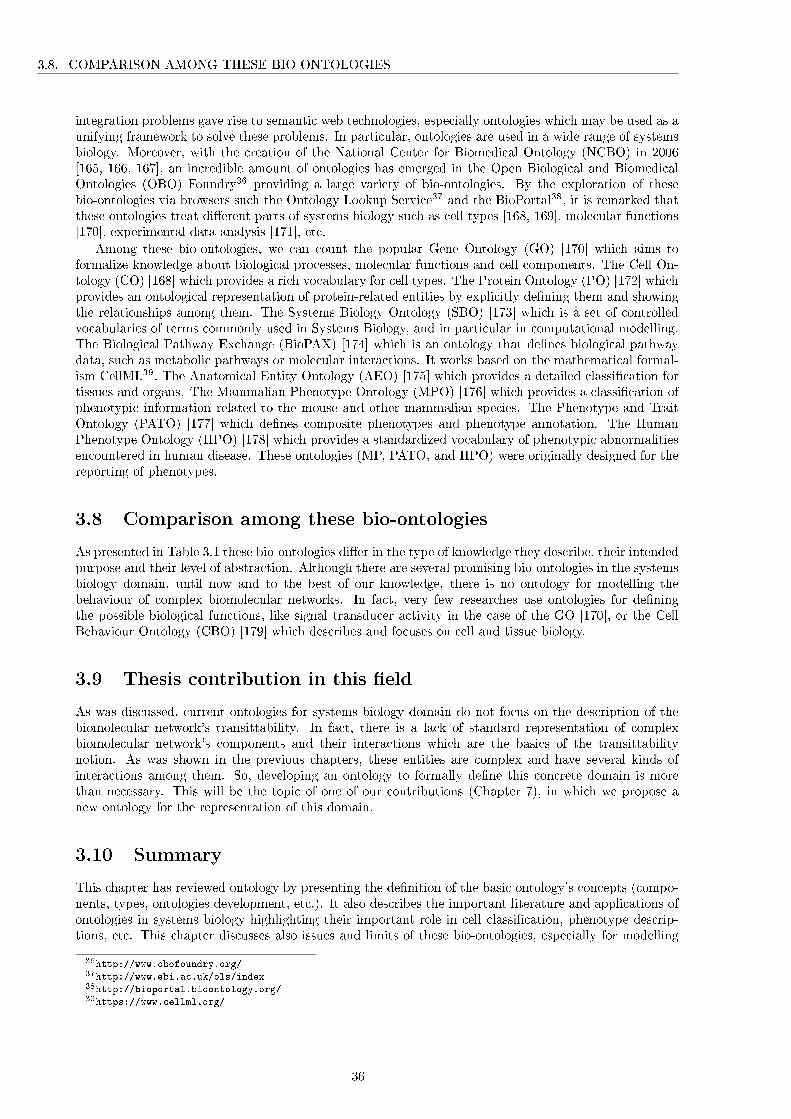
3.8. COMPARISON AMONG THESE BIO-ONTOLOGIES
integration problems gave rise to semantic web technologies, especially ontologies which may be used as aunifying framework to solve these problems. In particular, ontologies are used in a wide range of systemsbiology. Moreover, with the creation of the National Center for Biomedical Ontology (NCBO) in 2006[165, 166, 167], an incredible amount of ontologies has emerged in the Open Biological and BiomedicalOntologies (OBO) Foundry36 providing a large variety of bio-ontologies. By the exploration of thesebio-ontologies via browsers such the Ontology Lookup Service37 and the BioPortal38, it is remarked thatthese ontologies treat di�erent parts of systems biology such as cell types [168, 169], molecular functions[170], experimental data analysis [171], etc.
Among these bio-ontologies, we can count the popular Gene Ontology (GO) [170] which aims toformalize knowledge about biological processes, molecular functions and cell components. The Cell On-tology (CO) [168] which provides a rich vocabulary for cell types. The Protein Ontology (PO) [172] whichprovides an ontological representation of protein-related entities by explicitly de�ning them and showingthe relationships among them. The Systems Biology Ontology (SBO) [173] which is a set of controlledvocabularies of terms commonly used in Systems Biology, and in particular in computational modelling.The Biological Pathway Exchange (BioPAX) [174] which is an ontology that de�nes biological pathwaydata, such as metabolic pathways or molecular interactions. It works based on the mathematical formal-ism CellML39. The Anatomical Entity Ontology (AEO) [175] which provides a detailed classi�cation fortissues and organs. The Mammalian Phenotype Ontology (MPO) [176] which provides a classi�cation ofphenotypic information related to the mouse and other mammalian species. The Phenotype and TraitOntology (PATO) [177] which de�nes composite phenotypes and phenotype annotation. The HumanPhenotype Ontology (HPO) [178] which provides a standardized vocabulary of phenotypic abnormalitiesencountered in human disease. These ontologies (MP, PATO, and HPO) were originally designed for thereporting of phenotypes.
3.8 Comparison among these bio-ontologies
As presented in Table 3.1 these bio-ontologies di�er in the type of knowledge they describe, their intendedpurpose and their level of abstraction. Although there are several promising bio-ontologies in the systemsbiology domain, until now and to the best of our knowledge, there is no ontology for modelling thebehaviour of complex biomolecular networks. In fact, very few researches use ontologies for de�ningthe possible biological functions, like signal transducer activity in the case of the GO [170], or the CellBehaviour Ontology (CBO) [179] which describes and focuses on cell and tissue biology.
3.9 Thesis contribution in this �eld
As was discussed, current ontologies for systems biology domain do not focus on the description of thebiomolecular network's transittability. In fact, there is a lack of standard representation of complexbiomolecular network's components and their interactions which are the basics of the transittabilitynotion. As was shown in the previous chapters, these entities are complex and have several kinds ofinteractions among them. So, developing an ontology to formally de�ne this concrete domain is morethan necessary. This will be the topic of one of our contributions (Chapter 7), in which we propose anew ontology for the representation of this domain.
3.10 Summary
This chapter has reviewed ontology by presenting the de�nition of the basic ontology's concepts (compo-nents, types, ontologies development, etc.). It also describes the important literature and applications ofontologies in systems biology highlighting their important role in cell classi�cation, phenotype descrip-tions, etc. This chapter discusses also issues and limits of these bio-ontologies, especially for modelling
36http://www.obofoundry.org/37http://www.ebi.ac.uk/ols/index38http://bioportal.bioontology.org/39https://www.cellml.org/
36

3.10. SUMMARY
Table3.1�Description
ofsomepopu
larbiological
ontologies.
Biologicalontology
name
Content
Reference
Link
CellOntology(O
BO)
Cellulartypes
[168]
http://obofoundry.org/ontology/cl.html
GeneOntology(G
O)
Biologicalprocess
[170]
http://www.geneontology.org/
Protein
Ontology(PO)
Protein
entities
[172]
http://pir.georgetown.edu/pro/
System
sBiology
Ontology(SBO)
System
sbiologynomenclature
[173]
http://www.ebi.ac.uk/sbo/main/
BiologicalPathw
ayExchange(B
ioPAX)
Molecular
entities
[174]
http://www.biopax.org/
Anatomical
EntityOntology(A
EO)
Cellclassi�cation
[175]
http://bioportal.bioontology.org/ontologies/AEO
Mam
malianPhenotype
Ontology(M
PO)
Phenotypicqualities
[176]
https://www.ebi.ac.uk/ols/ontologies/mp
Phenotype
andTraitOntology(PATO)
Phenotypicqualities
[177]
http://agroportal.lirmm.fr/ontologies/PATO
Hum
anPhenotype
Ontology(H
PO)
Phenotypicqualities
[178]
http://human-phenotype-ontology.github.io/
CellBehaviorOntology(C
BO)
Cellularbehaviour
[179]
http://cbo.biocomplexity.indiana.edu/cbo/
37

3.10. SUMMARY
the behaviour of complex biomolecular networks, and suggests some approaches that might be useful inthe future.
Before detailing the proposed semantic modelling of biomolecular networks, the following chapter willreview background on simulation and optimization methods in systems biology.
38

Chapter 4
Simulation tools in systems biology
Contents4.1 Introduction . . . . . . . . . . . . . . . . . . . . . . . . . . . . . . . . . . . . . 40
4.2 Principles of simulation . . . . . . . . . . . . . . . . . . . . . . . . . . . . . . . 40
4.2.1 De�nition . . . . . . . . . . . . . . . . . . . . . . . . . . . . . . . . . . . . . . . 40
4.2.2 Relation between modelling and simulation concepts . . . . . . . . . . . . . . . 40
4.2.3 Uses of simulation . . . . . . . . . . . . . . . . . . . . . . . . . . . . . . . . . . 41
4.2.4 Levels of abstraction . . . . . . . . . . . . . . . . . . . . . . . . . . . . . . . . . 41
4.3 Overview of existing simulation tools in systems biology . . . . . . . . . . . 41
4.3.1 Mathematical and population-based simulation . . . . . . . . . . . . . . . . . . 42
4.3.2 Individual-based simulation . . . . . . . . . . . . . . . . . . . . . . . . . . . . . 42
4.3.3 Computational simulation platforms . . . . . . . . . . . . . . . . . . . . . . . . 43
4.3.4 Discrete Event System Speci�cation . . . . . . . . . . . . . . . . . . . . . . . . 45
4.4 Comparison among these simulation tools and platforms . . . . . . . . . . 46
4.5 Thesis contribution in this �eld . . . . . . . . . . . . . . . . . . . . . . . . . . 47
4.6 Summary . . . . . . . . . . . . . . . . . . . . . . . . . . . . . . . . . . . . . . . 49
39

4.1. INTRODUCTION
4.1 Introduction
Simulation of biomolecular networks is essential for studying biological systems from small reaction net-works to large sets of cells [180]. Models are useful for many di�erent purposes, among them testingtheoretical hypotheses, guiding experiments and looking at experimentally unreachable scenarios, as wellas the ability to predict new behaviours of these complex networks.
This chapter focuses on the notion of simulation with emphasis on its use in biological systems. The�rst section presents the principles and characteristics of the simulation theory. The second sectionreviews the most popular simulation tools and platforms in systems biology through a comparison study.We will also discuss the issues and limits of these simulations and de�ne the contribution of our thesis inthis �eld.
4.2 Principles of simulation
4.2.1 De�nition
The simulation is one of the most e�ective decision support tools available to designers and managers ofcomplex systems. It consists in constructing a model of a real system and performing experiments onthis model in order to understand the behaviour of this system and improve its performance.
Formally, the simulation is the imitation of a real-world process or the functioning of a system overtime [181]. Thus, a simulation can be de�ned as a representation of the functioning of a system or process.Through simulation, a model is implanted with unlimited variations producing complex scenarios. Thesecapabilities allow analysis and understanding of how individual elements interact and a�ect the simulatedenvironment.
Advances in computer science have signi�cantly increased the power of simulations. Computer sim-ulations are often based on iterative methods for calculating the detailed state of an entire system atthe instant t + 1 depending on its state at the instant t. They are holistic because they simultaneouslyconsider many properties of a system.
4.2.2 Relation between modelling and simulation concepts
The concept 'modelling ' has di�erent meanings: (i) modelling refers to all the activities of creation,development and execution of virtual models of the system to be studied. (ii) Modelling merges withnumerical simulation. (iii) Modelling is the development of relationships between the characteristicvariables of a given system, able to simulate the behaviour of that system in a given context.
In our research, we follow the third de�nition. In order to study the behaviour of a complex system,it is essential to distinguish between two di�erent phases: (i) the development of models and (ii) theiruse in a concrete study. Only the �rst phase is called modelling (which we have detailed in Chapter 2)and the second phase is called simulation (that is the main topic of this chapter). The use of modelsis not limited to the simulation. Thus, the simulation is one among several objectives of the modelling.The separation and distinction between the two phases contribute to the exchange of models and theirapplication.
As discussed in Chapter 2, the modelling aims to conceptualize the real world to �nd a relevantrepresentation of reality. This concept is developed through examples and generalizations based on logicalreasoning. In fact, every object in the real world has not a universal de�nition and does not depend totallyon a speci�c model. Everyone is able to provide a personal de�nition based on its ideas. Communicationbetween humans is only possible through common and shared parts of a concept. Thus, the main objectiveof modelling is the formal description of this concept (usually expressed in mathematical formalism). Inchapter 2, we have detailed these di�erent categories of mathematical models.
On the other hand, the simulation phase consists of one possible exploitation of this modelling. Thissimulation is guided by the objectives of its study by applying simpli�cations on the real properties of thestudied object. For a concrete system, the models developed during the modelling phase are used andapplied to its problem. It is at this stage that the simulation of the modelled system is used to obtainresults that are otherwise too di�cult to obtain.
40

4.3. OVERVIEW OF EXISTING SIMULATION TOOLS IN SYSTEMS BIOLOGY
4.2.3 Uses of simulation
Simulation is used in research to study the behaviour of complex systems, or systems composed of multipleinterdependent processes [182], and it can be used for a variety of research purposes [183] such as:
• Prediction: the simulation provides hypotheses about the future behaviour of a system or phenom-ena.
• Proof : the simulation con�rms the theoretical knowledge.
• Discovery : the simulation is used to predict and discover new unexpected consequences or knowl-edge.
• Explanation: the simulation is used to clarify the behaviours which are observed but their reasonsare unknown.
• Critique: the simulation can be used to explore, modify and correct the theoretical explanationsfor phenomena proposed by researchers.
• Prescription: the simulation can propose a better mode of operation or method of analysis.
4.2.4 Levels of abstraction
According to the aim of the simulation and the degree of detail of the behaviour analysis that the userwishes to simulate, diverse levels of abstraction are possible: macro, meso and micro levels.
• Themacro-simulations are simulations in which the system is studied as a whole without consideringlocal actions and interactions [184]. These simulations analyse global characteristics of the system.They are important when the real system is too complex and need to be divided into small elements.
• The meso-simulations do not study a system at a global or local level but use the aggregation oflocal elements and focus on the interactions among these aggregations [185]. These simulationsconstitute an intermediate level where local and global components are combined in the analysisof the system. They are used in the case of a system that is di�cult to qualify and quantify atlocal levels or when the user does not require �ne decomposition (when it is necessary to study theinteractions among the components of the system).
• The micro-simulations have gradually emerged in diverse �elds where scientists want to makeprogress in the detail, realism and understanding of system [186]. These simulations consider thesystem at its most local level.
In the case of meso-simulations and micro-simulations, the global behaviour is the implication of themost local levels and results from interactions among local components. Consequently, it is possible tocombine these di�erent levels of abstraction within the same simulation.
4.3 Overview of existing simulation tools in systems biology
There are two kinds of simulation tools based on the mathematical modelling approaches detailed inChapter 2: population-based models and individual-based models (called also agent models).
Population-based models describe the general behaviour of the whole system by the aggregation ofall the individual states and behaviours. These models are represented by a mathematical formalism(detailed in Chapter 2). They can not describe the behaviour of individual components independentlyof others. However, in order to simulate individual behaviours, it is necessary to use individual-basedmodels. These models are described by rules applying to each individual in order to manage theirbehaviour. These rules are simple or complex.
41

4.3. OVERVIEW OF EXISTING SIMULATION TOOLS IN SYSTEMS BIOLOGY
4.3.1 Mathematical and population-based simulation
Based on di�erent approaches for modelling biological systems, diverse platforms for the simulation oftheir properties have been developed.
These simulators started with the development of the BioProcess simulator (BPS) by Aspen Technol-ogy [187] in 1985. This simulator includes a number of operation modules speci�c for diverse biochemicalprocesses such as the ultra�ltration, the chromatography, etc. Inspired by the BioProcess, other simu-lators were developed such as the BioPro designer developed by the Biotechnology Process EngineeringCenter at the Massachusetts Institute of Technology (MIT) and completed by INTELLIGENT [188],the Environmental Simulation Program (ESP) developed by OLI systems, and the GPS-X [189] devel-oped by Hydromantis. All these simulators share the same characteristics of the BioProcess simulatorand are mostly developed to simulate macroscopic behaviour such as cell development and are based onunstructured models.
Other simulation tools to understand biochemical pathways in the cell, using a structured model ofthe system have been published by diverse academic groups. We can cite: KINSIM [190], MetaModel[191], Jarnac/SCAMP [192], MIST [193], Gepasi [194], DBsolve [195], ProMot/Diva [196] and BioSPICE[197]. All these simulator tools aim to simulate metabolic networks based on di�erential equations. Thesesimulations tools are basically designed to simulate structured, dynamic, and deterministic systems.
On the other hand, MetaFluxNet [198] has recently been developed to execute static simulationsused for metabolic analysis. This simulator interacts with users through standard SQL commands forquerying three databases: ENZYME [199], LIGAND [199] and EcoCyc [200]. Based on these threedatabases, MetaFluxNet allows users to develop metabolic models corresponding to their objectives.
Another type of mathematical modelling based on stochastic aspects is used for simulating geneexpression. In this category, we can cite the STOCKS simulator which is a software for stochasticsimulation based on the Gillespie algorithm [201]. This simulator was used for simulating the proteinsynthesis and mRNA levels of the LacZ gene of E. coli. Another simulator the StochSim [202] which isalso based on a stochastic simulation algorithm and a simple two-dimensional spatial structure. StochSimwas used to simulate the pathway controlling chemotaxis in E. coli [203].
4.3.2 Individual-based simulation
Among the popular individual-based models used for simulating biological systems, we have selectedthe Potts model, Lattice gas automata, Cellular automata and Multi-agent systems. There are severalreviews that cover the uses of these models for simulating biological systems, three of them were used inthe development of this section [204], [205].
4.3.2.1 Cellular Automata
This model was detailed in Chapter 2. Cellular automata were adopted in 1966 with the publicationof Von Neumann's book 'Theory of self-reproducing automata' [206]. Then they were popularized byJohn Conway through the Game of Life which was described in an article by Martin Gardner [207].Cell automata have been used to model diverse systems such as the developmental processes in biology[208, 209], the entire developmental lifecycle of the cellular slime mould Dictyostelium discoideum [210,211], the cell growth and cell death [212], and the cell polarity [213]. A detailed survey containing moreexamples simulated with cellular automata can be found in [205].
4.3.2.2 Multi-Agent Systems
As already detailed in Chapter 2, multi-agent systems are based on the modelling of interacting agents. Itis not necessary to model an environment because it is always modelled implicitly in the form of an agent.Each modelled agent have its own rules and there are several types of agents as detailed in Chapter 2.According to Grimm, multi-agent systems have two advantages. The �rst is characterised as 'pragmatic'and comes from the di�culty of studying complex behaviour using mathematical models. The secondreason is called 'paradigmatic' and it occurs when mathematical models show their limits to simulateand explain the regulation, emergence, resilience, persistence, etc. in ecosystems [214]. However, thereis no precise de�nition of a Multi-agent system and the evaluation of this model is delicate for lack oftools and methodology [215, 216]. There are many multi-agent model used to simulate systems in diverse
42

4.3. OVERVIEW OF EXISTING SIMULATION TOOLS IN SYSTEMS BIOLOGY
areas, such as ecology [217, 218], solving complex problems like the Travelling salesman problem [219]. Insystems biology, works focus on protein relocations [220], the immune system [221] and cellular functions[222].
4.3.2.3 Potts model
The Potts model was developed to model and simulate the spin interactions in the crystalline networks[223]. This model is sometimes described as a modi�ed cellular automaton. It consists of a regular matrixof cells and each cell have a value describing its state. The di�erence with the cellular automata is thatthe individual can cover several boxes (meshes) where an individual in the cellular automata can coveronly one box (mesh). In the Potts model, an individual is represented by a region of the matrix andthe boxes have a label that allows them to know to which individual they belong. The Potts model isrelated to and generalized by several other models including the XY model, the Heisenberg model andthe N-vector model. This model was used to analyse the tissue reorganization by self-organization of cellsaccording to the relationships among them [210, 224]. The Potts model is sometimes described as theCellular Potts Model or CPM [204].
4.3.2.4 Lattice gas automata
The Lattice-Gas system is called also interacting Particle System. This model was proposed by Hardy,Pazzis and Pomeau who were interested in �uid mechanics [225]. The Lattice-Gas model became knownin 1986 with the work of Frish, Hasslacher and Pomeau on the Navier-Stokes equation [226]. Lattice-Gassystem consists of a regular matrix in which each box (mesh) has several sites, each site corresponds toone direction called a channel. In the description of this system, the commonly used term is not a box(mesh) but we talk about a node. A particle placed in this network moves from a node to another throughthe channels corresponding to its direction. Each particle takes the information concerning its velocityto know how many nodes it must move in steps of time. This allows the management of collisions amongthe particles. This notion of the node to node moving makes the Lattice-Gas system closer to cellularautomata that's why many studies called it LGCA for Lattice-Gas Cellular Automata [226]. Collisionmanagement can be compared with the transition rules of a cellular automaton [205, 227]. A recentextension of the LGCA model considers continuous models instead of discrete entities and it is calledthe LBCA for Lattice Boltzmann Cellular Automata. This model was mainly used for the simulationof physical systems, such as �uid mechanics. Nevertheless, there are some interesting implementationsof biological systems simulation in hemodynamics [228, 229] and the metastasis formation in cancerdevelopment [230].
4.3.3 Computational simulation platforms
4.3.3.1 Simulation standard
SBML
System Biology Markup Language (SBML)1 is a modelling language project introduced by Hiroaki Kitano[48] in 2001 and derived from the XML standard. The SBML aims to standardize the biochemical processmodels. The �rst version was produced in 2001 [231] and published in 2003 [231]. Di�erent versions ofthe platform appeared like SBML Level 3 Version 1 Core in 2010 [232]. Some software are able to editmodels in SBML standards such as CellDesigner, V-Cell and Snoopy.
CellML
Similarly to the SBML, CellML2 is also a language project deriving from the XML standard. This projectis supported by the Bioengineering Institute of Auckland University. It was initially introduced by WarenHedley and Melanie Nelson [233] in 2000 on the Physiome project designed to model organ functioningfrom the cellular level. Some software are able to edit models in the CellML formats such as OpenCelland V-Cell.
1http://sbml.org/Main_Page2https://www.cellml.org/
43

4.3. OVERVIEW OF EXISTING SIMULATION TOOLS IN SYSTEMS BIOLOGY
4.3.3.2 Simulation tools
E-Cell
E-Cell3 is a project started in 1996 at the Laboratory for Bioinformatics at Shonan-Fujisawa Universityin Keio in Japan, under the name of ECL for Electronic Cell Laboratory. Actually, it is in its thirdversion. This platform was developed to model the biochemical processes of the cell. The objectiveof the platform's authors is to provide a model as precise as possible of a real cell and to describe thestructural characteristics of the cell taking into account its physic and chemistry reactions. E-Cell requiresmodels written in SBML or EML (E-Cell Model) languages. It has been used to model the mitochondrialmetabolism [234], the red blood cell metabolism [235] and the circadian rhythm in Drosophila under thein�uence of light [236].
CompuCell3D
CompuCell3D4 is available online in its version 3.7.2. This platform appeared in 2003 before beingo�cially introduced by Lzaguirre et al. in 2004 [237]. It derives from the work of François Graner andJames Glazier (CPM and Q-Potts) in 1992 [224, 238]. CompuCell3D is presented by its authors as amulti-model support because it is based on the parallel use of three components: a Potts model, a di�usionmanagement module, and a module that manage the continuous mathematical models. CompuCell3D isdeveloped for the study of morphogenesis and is based on the authors' expertise to model the cellularrearrangements directed by the forces acting on their surface, complemented by the consideration of cellgenetics and the presence of chemical substances in the environment. This platform requires modelswritten in CCML or CC3DML which are derived from the XML standard. CC3DML is an extension ofthe CCML language that allows the description of phenomena in 3 dimensions and CCML is limited to2 dimensions. CompuCell3D has provided convincing results in morphogenesis by reproducing patternscharacteristic of microbial evolution in [239], in embryogenesis by allowing simulation of the gastrulationprocess in the chicken embryo [240], and in the segmentation of the vertebrate embryo [241, 242]. Severalexamples of simulation done by this platform have been referenced by Maciej Swat [243].
SimCell
SimCell5 is a model based on a variant of cellular automata called dynamic cellular automata proposedby Wishart et al. [244]. This dynamic cellular automaton consists of cellular automata in which abox of the cellular automata represents at most one macromolecule or a multitude of small molecules.The rest of cellular automata characteristics describes a regular two-dimensional cellular automatonwith heterogeneous, probabilistic and synchronous functioning. This model is intended to be a generalstructure for simulating most cellular processes. SimCell has three steps: (i) create the network using thegraphical user interface, (ii) simulate the behaviour of this network using the cellular automata, and (iii)generate at any time during the simulation, graphs and tables to present the evolution of the di�erententities involved in the network. SimCell uses colours to model species, however, it contains 70 colours,therefore it is limited to 70 species. In addition, when the number of molecules is large, the clarity ofthe cellular automata becomes complicated. As well as the analysis of the graphs. SimCell is suitable forsimulating simple biochemical networks in a reduced environment. It gives good results to analyse theBrownian movement and highlight the role of luck in the proper functioning and regulation of cellularprocesses [244].
V-Cell
V-Cell6 has been developed by the CCAM (Center for Cell Analysis and Modeling) in 1997 and is basedon the work of Scha� et al. [245]. It is designed as a modelling tool for cellular processes for research incell biology. For this reason, it is able to model the di�erent nature of complex models (mathematical orempirical). V-Cell is comparable to SimCell in many characteristics. The di�erence between them is thatSimCell is constrained to 70 kinds of entities, however, there is no limit of entities for V-Cell. Moreover,
3http://www.e-cell.org/4http://www.compucell3d.org/5http://wishart.biology.ualberta.ca/SimCell/6http://vcell.org/
44
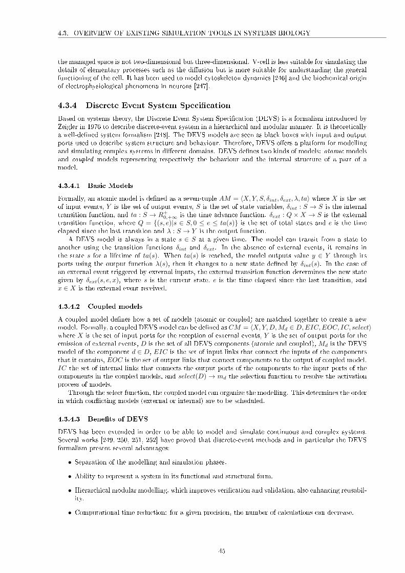
4.3. OVERVIEW OF EXISTING SIMULATION TOOLS IN SYSTEMS BIOLOGY
the managed space is not two-dimensional but three-dimensional. V-cell is less suitable for simulating thedetails of elementary processes such as the di�usion but is more suitable for understanding the generalfunctioning of the cell. It has been used to model cytoskeleton dynamics [246] and the biochemical originof electrophysiological phenomena in neurons [247].
4.3.4 Discrete Event System Speci�cation
Based on systems theory, the Discrete Event System Speci�cation (DEVS) is a formalism introduced byZeigler in 1976 to describe discrete-event system in a hierarchical and modular manner. It is theoreticallya well-de�ned system formalism [248]. The DEVS models are seen as black boxes with input and outputports used to describe system structure and behaviour. Therefore, DEVS o�ers a platform for modellingand simulating complex systems in di�erent domains. DEVS de�nes two kinds of models: atomic modelsand coupled models representing respectively the behaviour and the internal structure of a part of amodel.
4.3.4.1 Basic Models
Formally, an atomic model is de�ned as a seven-tuple AM = 〈X,Y, S, δint, δext, λ, ta〉 where X is the setof input events, Y is the set of output events, S is the set of state variables, δint : S → S is the internaltransition function, and ta : S → R+
0,+∞ is the time advance function. δext : Q×X → S is the externaltransition function, where Q = {(s, e)|s ∈ S, 0 ≤ e ≤ ta(s)} is the set of total states and e is the timeelapsed since the last transition and λ : S → Y is the output function.
A DEVS model is always in a state s ∈ S at a given time. The model can transit from a state toanother using the transition functions δint and δext. In the absence of external events, it remains inthe state s for a lifetime of ta(s). When ta(s) is reached, the model outputs value y ∈ Y through itsports using the output function λ(s), then it changes to a new state de�ned by δint(s). In the case ofan external event triggered by external inputs, the external transition function determines the new stategiven by δext(s, e, x), where s is the current state, e is the time elapsed since the last transition, andx ∈ X is the external event received.
4.3.4.2 Coupled models
A coupled model de�nes how a set of models (atomic or coupled) are matched together to create a newmodel. Formally, a coupled DEVS model can be de�ned as CM = 〈X,Y,D,Md ∈ D,EIC,EOC, IC, select〉where X is the set of input ports for the reception of external events, Y is the set of output ports for theemission of external events, D is the set of all DEVS components (atomic and coupled), Md is the DEVSmodel of the component d ∈ D, EIC is the set of input links that connect the inputs of the componentsthat it contains, EOC is the set of output links that connect components to the output of coupled model,IC the set of internal links that connects the output ports of the components to the input ports of thecomponents in the coupled models, and select(D) → md the selection function to resolve the activationprocess of models.
Through the select function, the coupled model can organize the modelling. This determines the orderin which con�icting models (external or internal) are to be scheduled.
4.3.4.3 Bene�ts of DEVS
DEVS has been extended in order to be able to model and simulate continuous and complex systems.Several works [249, 250, 251, 252] have proved that discrete-event methods and in particular the DEVSformalism present several advantages:
• Separation of the modelling and simulation phases.
• Ability to represent a system in its functional and structural form.
• Hierarchical modular modelling, which improves veri�cation and validation, also enhancing reusabil-ity.
• Computational time reduction: for a given precision, the number of calculations can decrease.
45

4.4. COMPARISON AMONG THESE SIMULATION TOOLS AND PLATFORMS
• Hybrid systems modelling: the discrete-event paradigm provides a uni�ed theory to model andsimulate systems with continuous and discrete components.
• Ability to be extended to new �elds of study or to be integrated into other modelling approaches(Petri nets, cellular automata, etc.).
The DEVS formalism has been used to simulate enzymes [253] and the tryptophan synthetase metabolicpathway [254].
4.4 Comparison among these simulation tools and platforms
Most of these simulation tools propose the use of complicated mathematical models that are composedof equations for simulating the behaviour of biomolecular systems. However, the mathematical modelsfor simulating the behaviour of biomolecular systems are sometimes complicated to solve considering thehigh number of molecular components and their heterogeneity. In fact, one of the major problems insimulating complex biological systems using mathematical models is the lack of quantitative data. Indeed,most of the biological knowledge available is qualitative but for quantitative simulation, a large amountof numerical data (such as concentrations of metabolites and enzymes, �ux rates, kinetic parameters anddissociation constants) is required.
Moreover, these methods do not follow individuals over time, instead, they track only total popu-lations. They also consider that the interactions among molecular components are homogeneous andassume that the entire system is just the sum of its components which is not necessarily true.
Others simulation tools such as Boolean and logic networks are suited to simulate the small networkand particularly Gene Regulatory Networks and signalling pathways. However, it becomes impracticalto simulate large biomolecular network sizes (for n nodes, we have 2n possible states).
Despite mathematical methods, we have also focused on individual-based models such as cellularautomata, Potts models, Lattice gas models, multi-agent models, etc. Both can be considered as cellularautomata and they have the same characteristics. These models respond to the simulation of complexsystems and are a suitable tool for studying the behaviour of such systems. The advantages of thiskind of simulation tools are that they are easy to implement and simple in design. But the interactionsand relationships among individuals are complex. Multi-agent models provide a detailed description ofcomplex systems. However, if they provide a high level of detail, their design generates a high cost.As well as, the disadvantages of such systems consist of the inability of agents to the more complexorganization and the excess parallelism of task's execution. This creates di�cult and obscure models.
Others simulation tools such as SimCell, are respectively based on the cellular automata and a discretemodel was totally designed for analysing the response of each individual in a population (respectively,each component in the biological system) and how this individual contributes within the population.Thus, these models focus only on the equilibrium and regulation of populations through interactionsthat exist among their individuals under the constraints of the environment. These models focus onlyon reproducing the modi�cation of individuals over generations under the constraints of environmentalchange or competition among individuals. Consequently, they aim only on the evolution of systems atthe population scale. Thus, we can conclude that all these simulation tools are dedicated to very speci�cproblems.
On the other hand, some platforms are designed to treat di�erent problems, such as V-Cell. Thesegeneric platforms require that the system must be formalized under the required standard formalism tobe simulated. Among these speci�c standards, we have discussed the SBML and CellML correspondingrespectively to the V-Cell and Snoopy platforms. The limit of these generic platforms is that they cannot simulate multi-level models. They are designed to address only a speci�c level of the system thattypically takes place at a given time and place. Therefore, they can not focus on the interactions amongthe di�erent omics levels.
We also discussed another formalism the discrete-event system speci�cation for coupling di�erentheterogeneous data models, di�erent levels of a system, speci�cation of sub-models of the system in asingle formalism, etc. Under the DEVS formalism, the behaviour of the whole system is easier to simulateif it is represented by a set of states that characterize the individual's activity. In this formalism, a de�nitetype of response of the individual to external stimulus corresponds to a set of states. Moreover, thesestimuli are generally not represented by continuous functions in the environment but by occasional events.
46

4.5. THESIS CONTRIBUTION IN THIS FIELD
In its original version, DEVS formalism allows the speci�cation of event status changes and provides amodular and hierarchical view of dynamic systems. So, we think that it is the most suitable for simulatingcomplex biological systems.
Table 4.1 provides a comparison of all these methods according to their characteristics. Indeed, wecompare these di�erent simulation methods based on various criteria, such as
• The abstraction level focuses on the level of detail (macro-, meso- and micro-levels).
• The topic interest focuses on the interested subject (speci�c to a subject or general to diversetopics).
• The network size focuses on the size of the biomolecular network (small- or large-scale).
• The category focuses on the type of the simulation (discrete, continuous or stochastic).
• The data type focuses on the type of data to be simulated (qualitative or quantitative data).
• The dynamic simulation focuses on the level of details of the simulation (local or global vision)
• The di�culty level focuses on the complexity with which the model can be understood and manip-ulated (easy or hard).
• Cost : includes all the charges for design, implementation, operation and maintenance (low or highcost).
After discussing all the properties of these simulation methods, we note that no method is betterthan the rest, only more suitable for a certain problem. Each of these tools has its own uses and is bestsuited for solving problems of certain scale and complexity. However, most of these methods considerthe biomolecular network as a simple network usually taking account only one level by focusing onlyon modelling isolated parts of this network, such as metabolic networks, gene regulation networks, andprotein-protein interaction networks. However, the interconnection among these di�erent network levelsre�ects the importance of a general approach that focuses on the multi-level properties of biomolecularnetworks to replace these traditional methods. In practice, qualitative models and quantitative modelscomplement each other. The choice between qualitative models and quantitative models depends on theavailability of kinetic information, the size of the systems and the types of questions to be addressed.
So, we conclude that the choice of a simulation method is determined by the characteristics of thesystem in which we are interested, how realistic an estimation of it we want, and our mathematical andcomputational resources. Thus, all of these simulation methods can be used but each method incorporatesdi�erent levels of detail and requires di�erent computational e�ort.
4.5 Thesis contribution in this �eld
The whole behaviour of the cell is an emergent behaviour of many component's interactions (such as DNA,proteins, and metabolites) belonging to di�erent levels (genome, proteome and metabolome). That iswhy, after the detailed comparison presented above, we conclude that it is not enough to simply describethe system's components or to only simulate a speci�c level such as genetic or metabolic level, etc. Indeed,there are still many di�culties that inhibit the construction of a complete simulation method. Therefore,in order to understand the global behaviour of biological systems, it is also necessary to detail the localbehaviour of each component at the molecular level and to understand what happens when certainexternal stimuli or intern malfunctions occur. So, rather than the previous approaches which focuson traditional reductionist methods, we think that the behaviour of the complex biomolecular networkemerges from the network-level interactions and requires an integrative simulation tool. That is why wewill propose in Chapter 8 a simulation approach based on the DEVS formalism and combines logical-based modelling and qualitative simulation. This simulation approach will consider all the omic-levelsand will be able to predict and reproduce the behaviour of the biomolecular network and its componentsunder a wide variety of stimuli or stresses.
47

4.5. THESIS CONTRIBUTION IN THIS FIELD
Table
4.1�Com
parisontable
ofthe
main
approachesapplied
tosim
ulatebiological
networks
accordingto
theircharacteristics.
vMathem
atica
land
Individ
ual-ba
sedPlatfo
rmsim
ulatio
nDEVS
populatio
n-ba
sedsim
ulatio
nsim
ulatio
nspeci�
cplatfo
rms
generic
platfo
rms
Abstra
ctionlevel
macro
%%
%
meso
%
micro
%%
%
Topic
interest
speci�cto
aproblem
%%
%%
genera
l(di�eren
tprob-
lems)
%%
Netw
ork
sizesm
all-sca
le%
%%
%%
large-sca
le%
%%
Catego
rydiscrete
%%
stochastic
%%
%%
contin
uous
%%
%%
Data
type
quantita
tive%
%%
%%
qualita
tive%
%
Dynamic
simulatio
nglo
balvisio
n%
%%
%
localvisio
n%
Di�
culty
leveleasy
%%
%%
hard
%%
Cost
low
%%
high
%(dependsonthemodel)
%%
%
48

4.6. SUMMARY
4.6 Summary
This chapter presented the principles (de�nitions, uses, levels of abstraction, etc.) that characterize theconcept of simulation in general. It also detailed the di�erent simulation tools and platforms in di�erentcategories and for di�erent purposes. In fact, each simulation uses a model that makes it possible tostudy a particular phenomenon and explain the performance of the simulation results in relation to thereal phenomenon and the user's desired objective. This state-of-the-art reveals the limitations of somesimulation tools based on mathematical modelling (due to their enormous size it becomes complicated tode�ne exactly their parameters).
49

4.6. SUMMARY
50

Chapter 5
Optimization tools in systems biology
Contents5.1 Introduction . . . . . . . . . . . . . . . . . . . . . . . . . . . . . . . . . . . . . 52
5.2 Optimization problem: de�nition and basic concepts . . . . . . . . . . . . . 52
5.2.1 De�nition . . . . . . . . . . . . . . . . . . . . . . . . . . . . . . . . . . . . . . . 52
5.2.2 The objective function . . . . . . . . . . . . . . . . . . . . . . . . . . . . . . . . 53
5.2.3 The vector of decision variables . . . . . . . . . . . . . . . . . . . . . . . . . . . 53
5.2.4 Constraints and delimitation of the research space . . . . . . . . . . . . . . . . 53
5.2.5 The di�erent types of optimum points . . . . . . . . . . . . . . . . . . . . . . . 53
5.3 Classi�cation of optimization problems . . . . . . . . . . . . . . . . . . . . . 54
5.4 Mono-objective optimization problem . . . . . . . . . . . . . . . . . . . . . . 55
5.5 Multi-objective optimization problem . . . . . . . . . . . . . . . . . . . . . . 55
5.5.1 Dominance relation . . . . . . . . . . . . . . . . . . . . . . . . . . . . . . . . . . 56
5.5.2 Pareto-optimal solutions . . . . . . . . . . . . . . . . . . . . . . . . . . . . . . . 56
5.6 Optimization methods . . . . . . . . . . . . . . . . . . . . . . . . . . . . . . . 57
5.6.1 The methods based on a metaheuristic approach . . . . . . . . . . . . . . . . . 57
5.7 Optimization problems in system biology . . . . . . . . . . . . . . . . . . . . 62
5.7.1 Optimization in the design of optimal dynamic experiments . . . . . . . . . . . 62
5.7.2 Optimization in the parameter estimation in cell systems modelling . . . . . . 62
5.7.3 Optimization in biological network alignment . . . . . . . . . . . . . . . . . . . 63
5.7.4 Optimization of biochemical reaction networks . . . . . . . . . . . . . . . . . . 63
5.7.5 Optimization in the sequence alignment problem . . . . . . . . . . . . . . . . . 63
5.7.6 Optimization in inferring networks . . . . . . . . . . . . . . . . . . . . . . . . . 63
5.7.7 Optimization in the network controllability . . . . . . . . . . . . . . . . . . . . 64
5.8 Comparison among these optimization tools and problems . . . . . . . . . 64
5.9 Thesis contribution in this �eld . . . . . . . . . . . . . . . . . . . . . . . . . . 65
5.10 Summary . . . . . . . . . . . . . . . . . . . . . . . . . . . . . . . . . . . . . . . 65
51

5.1. INTRODUCTION
5.1 Introduction
Optimization is a rapidly growing discipline that a�ects various research �elds, such as vehicle routingproblems, scheduling problems, assignment problems, air tra�c problems, etc. but also satisfy the needsof system biology. The optimization of these systems allows �nding an ideal con�guration for savinge�ort, time, money, energy or improving satisfaction. Some real-world problems require the simulta-neous optimization of several criteria which can sometimes be contradictory. This is the case of thetransittability of complex biomolecular networks that can be considered as multi-objective optimizationproblems.
In this chapter, we present the state of the art of optimization methods in general and multi-objectiveoptimization methods in particular. The �rst section presents some background de�nitions about theoptimization concept and its basic components. Next, we give the di�erent classi�cation of optimizationproblems according to their characteristics by focusing on mono and multi-objective optimization prob-lems. Then we present the popular optimization methods for solving multi-objective problems. Moreover,we review the major applications of optimization problems in systems biology through a comparison study.Finally, we discuss the contribution of our thesis to understand the transittability of complex biomolecularnetworks.
5.2 Optimization problem: de�nition and basic concepts
In this section, we will de�ne all the basic components of the optimization problem. To do this, we referto many literature reviews detailing these notions and available in [1, 255, 256].
5.2.1 De�nition
An optimization problem is de�ned as a problem that aims to search the minimum or maximum (theoptimum) of a given function f , so-called objective function [257].
According to M. Ejday [257] the optimization concept consists of two steps. These steps are illustratedin Figure 5.1.
• A �rst modelling step in which the user de�nes the objective function, the main optimizationvariables so-called decision variables, and the equality and inequality constraints. In the nextsections, we will detail these concepts.
• The second step of resolution consists in the search for the best values by optimizing the objec-tive function de�ned in the �rst modelling step. This resolution is done through an optimizationalgorithm [258].
Figure 5.1 � Modelling and resolution steps of an optimization problem.
Optimization has been introduced in order to improve the services provided regardless of their appli-cation areas. Indeed, the need for optimization comes from the engineer's need to provide the user with asystem that best meets its requirements. This system must be designed to (i) use the minimum necessaryfor its functioning (a minimum cost of resources), (ii) consume less energy (minimum operating cost),and (iii) respond to the user's request (satisfy all requirements).
This section de�nes some basic concepts of optimization theory. To do this, we have used these works[1, 255, 257, 256] to give some de�nitions of these notions.
52

5.2. OPTIMIZATION PROBLEM: DEFINITION AND BASIC CONCEPTS
5.2.2 The objective function
The objective function called also cost function or optimization criterion denoted by f is used in math-ematical optimization to describe a function that the optimization algorithm will have to optimize (�ndan optimum). This function represents the goal that the decision-maker wishes to achieve, and it is alsoused for measuring the goodness of values for the decision variable.
5.2.3 The vector of decision variables
The decision vector X is composed of the di�erent decision variables of the problem. These variablesexpress qualitative or quantitative data that need to be determined in order to solve the given problem.A decision variable is denoted by x ∈ X and can be a number, vector, function, etc. It is by changingthe values in this vector that an optimum of the function f is obtained.
5.2.4 Constraints and delimitation of the research space
There are two types of constraints: inequality constraints denoted by the vector g(x) and inequalityconstraints denoted by the vector h(x). These sets of constraints de�ne a restricted space for �nding theoptimal solution.
We distinguish two kinds of inequality constraints:
• Constraints of type Biinf ≤ x ≤ Bisup: the values of the decision variables that validate theseconstraints de�ne the research space or state space. This space is the space of all possible andcomplete solutions for the optimization problem. This space is �nite and de�ned by the domainsof de�nition of the di�erent decision variables of the problem (Figure 5.2a).
• Constraints of type c(x) ≤ 0 or c(x) ≥ 0: the values of the decision variables that check theseconstraints de�ne the space of the achievable values. This space is shown in Figure 5.2b.
(a) (b)
Figure 5.2 � Example of merging: 5.2a The research space. 5.2b The achievable space.
5.2.5 The di�erent types of optimum points
For a given function f , there may be few points at which the function reaches larger (or smaller) valueswhich may be higher (or lower) within some given neighbourhood. The higher points are called relativemaxima (or local maxima), while the lower points are called as relative minima (or local minima). Withina given interval, a function must have one (or more) highest and lowest point(s)1. As well as, the highestpoint is called global maximum and the lowest point is called global minimum [1, 259].
1https://math.tutorvista.com/statistics/global-minimum.html
53

5.3. CLASSIFICATION OF OPTIMIZATION PROBLEMS
In the following sections, we will only consider the problem of minimization. In fact, the problem ofmaximization follow the same rules. Here, we treat the case of the minimization without losing generalitybecause maximizing fi means minimizing −fi. Since, for example if f is a numerical objective function,maximizing (f) is same as minimizing (−f).
5.2.5.1 Local maximum and minimum
Optimization functions can have 'hills and valleys': places where they reach a minimum or maximumvalue. It may not be the minimum or maximum for the whole function, but only for a local interval.
Local minimum
First, we need to choose an interval. Then we can say that a local minimum is the point where the heightof the function at a is smaller than (or equal to) the height anywhere else in that interval. Formally, ifand only if f(a) ≤ f(x) for all x in the interval.
Formally, a point x∗ is a local minimum of the function f only if f(x∗) ≤ f(x) for all x ∈ V (x∗),where V (x∗) de�nes the interval of a neighborhood of the point x∗. This de�nition corresponds to pointsM1 M2 and M4 in Figure 5.3.
Local maximum
Likewise, a local maximum is the point where the height of the function at a is greater than (or equal to)the height anywhere else in that interval. Formally, if and only if f(a) ≥ f(x) for all x in the interval.
5.2.5.2 Global maximum and minimum
The maximum or minimum over the entire function f is called a Global maximum or minimum. Formally,a point x∗ is a global minima only if f(x∗) ≤ f(x), for all x in the domain of f . This de�nition correspondsto the point M3 in Figure 5.3.
Figure 5.3 � Global minimum and local minima [1].
5.3 Classi�cation of optimization problems
According to [1], the di�erent optimization problems are classi�ed according to their characteristics asfollows:
• Number of decision variables:
� One =⇒ single-variable or mono-objective optimization problem.
� Multiple =⇒ multi-variable or multi-objective optimization problem.
• Type of decision variables:
� Continuous real number =⇒ continuous optimization problem.
54

5.4. MONO-OBJECTIVE OPTIMIZATION PROBLEM
� Integer number =⇒ discrete optimization problem.
� Permutation on a �nite set of numbers =⇒ combinatorial optimization problem.
• Type of the objective function:
� Linear function of the decision variables =⇒ linear optimization problem.
� Quadratic function of the decision variables =⇒ quadratic optimization problem.
� Non-linear function of decision variables =⇒ non-linear optimization problem.
• Formulation of the problem:
� With constraints =⇒ constrained optimization problem.
� Without constraints =⇒ unconstrained optimization problem.
Indeed, there are di�erent types of optimization problems that depend on the number and typeof the decision variables, the type of the objective function (linear, quadratic or non-linear) and theformulation of the problem (with or without constraints). In addition to these characteristics, the numberof optimization objectives divides optimization problems into two major kinds. In this chapter, wefocus on these two categories of optimization problems: mono-objective optimization and multi-objectiveoptimization. In the following sections, we present the main concepts that are related to them. Moreover,we de�ne some optimization methods for solving these problems.
5.4 Mono-objective optimization problem
Mono-objective optimization consists of one and only one objective or criterion to be optimized. Thisis a category of optimization problems that are generally 'easy' to solve. The term easy here is used not todenote the level of di�culty of this type of problems but their di�culty in comparison with multi-objectiveproblems [1]. Indeed, mono-objective problems do not present a con�ict of interest in focusing on one ofseveral optimization criteria in contrast to multi-objective problems that have to consider several criteria.
Mono-objective optimization seems easy, but they have also di�culties such as the non-linear objectivefunction that cannot be expressed analytically in terms of parameters. In fact, modelling the problemin the form of a single equation can be a very di�cult task. Moreover, reducing the mathematicalformulation of the problem to a single objective function can lead to errors and mistakes in the modelling.This problem does not exist in the multi-objective optimization where a certain degree of �exibility isallowed [1].
A mono-objective optimization problem is mathematically de�ned as:Minimize/Maximize f(x) (function to be optimized)with g(x) ≤ 0 (inequality constraints)
With x ∈ Rm, g(x) ∈ Rp and h(x) ∈ Rq.
5.5 Multi-objective optimization problem
Most real optimization problems are described by several criteria frequently contradictory and whichmust be optimized simultaneously [255]. Multi-objective optimization aims to optimize these multitudesof objectives at the same time considering that they can be contradictory and generate con�icts ofinterest. These objectives can be explicitly de�ned as objective optimization criteria or formulated asconstraints. Formally, a multi-objective optimization problem is de�ned by the triplet (X,F, g) thatconsists in minimizing F (X) for X ∈ X with g(X) ≤ 0, and mathematically de�ned as follows:
Minimize F (X) = (f1(X), f2(X), . . . , fn(X)) (functions to be optimized)for X ∈ Xwith g(X) ≤ 0 (inequality constraints)
With x ∈ Rm,F (X) ∈ Rn , g(x) ∈ Rp and h(x) ∈ Rq.The m decision variables are the values to be chosen in an optimization problem. These values
are denoted by xi with i ∈ {1, . . . ,m}. The vector X of the m decision variables is denoted by X =(x1, x2, ..., xm). The set of decision variable vectors form the search space X . The n objective functions
55

5.5. MULTI-OBJECTIVE OPTIMIZATION PROBLEM
to be optimized are denoted by fi with i ∈ {1, . . . , n}. The vector F of the n objectives (for X ∈ X )is represented by F (X) = (f1(X), f2(X), . . . , fn(X)). The p inequality constraints and the q equalityconstraints limit the values that the decision variables can take. They are respectively denoted by gi(X)with i ∈ {1, . . . , p} and hi(X) with i ∈ {1, . . . , q}.
As discussed above, a multi-objective optimization problem has the advantage of providing a level of�exibility which is absent in mono-objective optimization. In addition, this �exibility a�ects the space ofsolutions by changing it from a single solution to several solutions. As well as, this space depends on theadopted optimization approach. Indeed, the objectives are sometimes contradictory, therefore, optimizingone objective can negatively a�ect one or more others. As a result, an optimal solution does not existbut we are talking about optimized solutions because multi-objective optimization cannot optimize allthe objectives at the same time and should give the priority to only some of them. It is in this casethat the concept of compromise is introduced because certain objectives will be preferred (optimized)to the exclusion of others having a bad quality performance. These solutions are considered useful andappropriate according to the user requirements.
Thus, in contrast to the mono-objective optimization problem, where the optimum is not a simplepoint but a set of points so-called the set of the best compromises or Pareto Front which is an area ofsolutions that o�er a good compromise between the di�erent objectives [1]. Therefore, the optimalityin a multi-objective context is based on the notion of dominance relation and Pareto-optimal (e�cient)solution. We will recall their de�nitions in the following sections.
5.5.1 Dominance relation
In multi-objective optimization problem, the solutions extracted are called Pareto solutions and constitutethe surface of compromise. The goodness of a solution is determined by the dominance relation. A solutionx1 dominates another solution x2 (noted x1 ≺ x2) if both the following conditions are true:
• Solution x1 is no worse than x2 in all objectives.
• Solution x1 is strictly better than x2 in at least one objective.
x1 ≺ x2{fi(x1) ≤ fi(x2) ∀i ∈ 1, . . . , n∃j ∈ 1, . . . , n fj(x1) < fj(x2)
Solutions that dominate the others but are not dominate themselves are called non-dominated solutions.Through this de�nition, the dominance relation is considered as a �lter of the bad elements to keep onlysolutions that cannot be compared with each other.
5.5.2 Pareto-optimal solutions
A number of criteria distinguish the selected solutions called Pareto-optimal solutions (or non-dominatedsolutions) when they are not dominated by any other solutions in the feasible space. The non-dominatedset of the entire feasible decision space is called the Pareto-optimal set. The boundary de�ned by the setof all point mapped from the Pareto-optimal set is called the Pareto-optimal front.
Like there are global and local optimum in the case of mono-objective optimization, we can also de�neglobal and local Pareto-optimal sets in multi-objective optimization. According to [256] we have:
• Local optimality in the Pareto sense: A solution x1 is locally optimal in the Pareto sense, if thereexists a positive real ε > 0 such that there is no other solution x2 that dominates the solution x1,with x2 ∈ Rm ∩B(x1, ε), where B(x1, ε) shows a bowl having a center x1 and a radius ε.
• Global optimality in the Pareto sense: A solution x1 is globally optimal in the Pareto sense, if theredoes not exist any vector x2 that dominates the vector x1.
The main di�erence between the global and local optimality lies in the fact that we do not have arestriction on the set Rm anymore. Thus, the Pareto set or the e�cient set is the collection of allPareto-optimal solutions and their corresponding images in the objective space is called the Pareto front.
These solutions are obtained using a precise approach based on a speci�c optimization method amonga wide range of techniques available in the literature [2]. The choice of the method to be applied must beadapted to the optimization problem to be solved. This choice represents a signi�cant di�culty becauseit is responsible for the success or not of the adopted method.
In the following, we focus on the optimization methods that can be used in this context.
56

5.6. OPTIMIZATION METHODS
5.6 Optimization methods
As discussed in the previous section, depending on the case (whether a single-variable or multi-variable,continuous or discrete problem, etc.), an appropriate optimization method is carefully chosen to solve theproblem in an e�cient way [259]. Several methods have been developed to solve mono-objective problemssuch as exact, heuristics, meta-heuristics, hybrid, etc. [2]. However, not all of them are appropriate forthe multi-objective optimization problems, therefore a reasonable choice should be made according to thenature and complexity of the given problem.
There are di�erent classi�cations of these various optimization methods for solving multi-objectiveoptimization problems in literature. According to DA Van Veldhuizen [260], optimization methods canbe grouped into four main categories:
• No preference methods which are methods where the decision maker is not considered and theproblem is saved using a simple method that presents directly the solution to the decision maker.
• A priori optimization methods which are methods where the compromises and preferences that wewould like to optimize are determined before the execution of the optimization method. In thismethod, the preferences of the decision maker are asked and then the best solution according tothe given preferences is found.
• A posteriori methods which aim to generate a representative set of Pareto-optimal solutions andthe decision maker chooses the best one among them. This method allows the decision maker tochoose the solution that is suitable for his problem by comparing it with the rest of the solutions.
• Interactive methods called also progressive optimization methods allow the interaction of the decisionmaker during the optimization process. This interaction is done by asking questions with thedecision maker.
In the following sections, we will only present the most used methods. To do this we follow theclassi�cation proposed by Colette et al. in their work [1] to group all the optimization methods into fourcategories: the interactive methods, scalar methods, fuzzy methods, and methods based on metaheuris-tics.
• Interactive methods: As discussed in the previous section, these methods are considered as pro-gressive methods which allow searching a single solution. They are based on the interaction withthe decision maker who can choose the solution that best corresponds to his preferences. In thiscategory, we cite the STEP method, the substitution compromise method, the Fandel method, etc.
• Scalar methods: They include a set of methods which are the most evident approach for solvingmulti-objective optimization problems. This approach called `naïve approach' aims to reformulatethe optimization problem in order to return to a mono-objective optimization. This process isfrequently achieved by using the aggregation (or the sum) of all objective functions in a singlefunction. A weighting coe�cient is assigned to each objective function to indicate its importancein the global objective function. By aggregating these weighted objective functions, we obtain asingle objective function. In this category of methods, we can also �nd the Keeney-Rai�a method[261], the distance to a reference objective method, etc.
• Fuzzy methods: These methods are inspired by fuzzy logic theory. They aim to neglect the binarylogic (true or false) and consider a certain degree of �exibility in order to accept the uncertaintyand imprecision of human knowledge. In this category, we �nd the Sakawa method, the Reardonmethod, etc.
For more detail, we can refer to the works of Colette et al. [1] in which they list, detail and formalizeall these methods.
5.6.1 The methods based on a metaheuristic approach
These methods have been developed since the 1980s. They include tabu search methods, simulatedannealing, genetic algorithms, ant colony algorithms, etc. The concept of metaheuristic was introduced
57

5.6. OPTIMIZATION METHODS
by Fred Glover in [262] who de�ned it as follows: 'A metaheuristic refers to a master strategy that guidesand modi�es other heuristics to produce solutions beyond those that are normally generated in a questfor local optimality '. As well as, another de�nition was proposed in [263], 'metaheuristics are solutionmethods that orchestrate an interaction between local improvement procedures and higher level strategiesto create a process capable of escaping from local optima and performing a robust search of a solutionspace'.
Their major objective is to solve di�cult optimization problems. In fact, metaheuristics were initiallydedicated to solving the di�culty of optimization problems. In contrast to traditional optimizationmethods (which take the path of the biggest slope to quickly �nd the local minima, but once they get theyfound the local minimum they do not search anymore), the main advantage of these methods is their abilityto avoid local minima. In fact, traditional methods start from an initial con�guration and search for thebest value through a series of iterations, while metaheuristics tolerate the momentary deterioration of thesituation. This idea has proven to be e�ective in avoiding local minima (or maxima) for solving complexproblems and become the basis of all neighbourhood metaheuristics (simulated annealing, tabu search,etc.). There are also other metaheuristics so-called distributed metaheuristics, such as evolutionaryalgorithms which also have very particular techniques to solve local minima (or maxima) problems.
In the next sections, we review metaheuristics cited above introducing their properties and functioning.
5.6.1.1 Simulated annealing
The simulated annealing method [264] is inspired by the annealing process and based on the principle ofstarting from a given con�guration to achieve the desired result. This result concerns the global optimum(or a result that is close to it) achieved by applying elementary transformations into a �nite number ofiterations.
In practice, this method uses the Metropolis algorithm which de�nes and represents the behaviourof a system in thermodynamic equilibriumat a speci�c temperature (T ) [264]. Starting from a givencon�guration, this method changes the system by modifying its basic elements such as the translation ofa component or the exchange of two components. If this modi�cation generates an improvement to thedesired objectives (for example a reduction of the objective function), it is accepted. On the other hand,even if this same change leads to a deterioration, it will be accepted but only with a certain probabilityof e−δE/T . Much that the higher the temperature, the more highly to keep the deteriorated state. Thisprocedure is repeated by keeping the temperature T constant until the thermodynamic equilibrium isreached after a number of iterations. Once this goal has been reached, the whole process is repeated fora new lower temperature value. A series of transformations is then performed on this value again.
Figure 5.4 presents the main steps of the simulated annealing algorithm [265]. In this �gure, theprocess described above is summarised and presented under a diagram summarizing the main stepsfollowed when applying an optimization method based on simulated annealing. There are several variantsof the simulated annealing method such as the simulated di�usion, micro-canonic annealing, thresholdmethod, �ooding method or record-breaking trip method.
5.6.1.2 Tabu search
The tabu search method was formalized in 1986 by F. Glover in [266]. The main advantages of thismethod are based on techniques inspired by human memory. In contrast to the simulated annealingmethod which is completely devoid of memory, the tabu search saves the history of the di�erent steps ofits application. It is able to react based on the lessons of the past. The actions performed in the currentiteration are a�ected by the previous actions that constitute the history of its execution. In addition,the tabu search method is simple. In fact, its procedure is similar to the simulated annealing methodand consists in applying a series of changes to several iterations of the process. The tabu search methodworks with only one con�guration at the same time. Initially, this con�guration is obtained arbitrary andthen locally updated (only small changes at each step). At each iteration, the mechanism of switchingfrom a given con�guration c to a successor con�guration c
′follows these steps [267]:
1. The construction of all the neighbours of c. This set represents all possible and achievable con�gura-tions accessible in a single elementary movement applied to c. If this set is too large, a well-de�nedtechnique is applied to reduce its size. Among these techniques: the selection of a list of candidates
58

5.6. OPTIMIZATION METHODS
Figure 5.4 � Diagram illustrates the process of the simulated annealing [2].
or the random extraction of a subset of �xed-size neighbours. V (c) denotes the set (or the subset)of these neighbours.
2. The evaluation of the objective function f in each of the con�gurations belonging to V (c). In termsof optimizing the objective function, the con�guration c
′that succeeds c would be the best among
those constituting the set V (c). In addition, this same con�guration c′can be taken into account
even if it proves to be less good than the �rst one c ( f(c′) > f(c)). This emphasizes the particularity
that constitutes the main advantage of metaheuristics (especially the tabu search method in thiscase) which consists in avoiding the local minima (or maxima) of the objective function f .
This procedure is sometimes ine�ective because there is a frequent risk of returning to a previous con-�guration already retained in a previous iteration. This generates a cycle and consequently the blockageon an in�nite loop. In order to avoid this problem, the tabu search method introduces the concept of theprohibited actions resulting in the construction of a list of prohibited movements. At each iteration, thislist which is continuously updated is used. The tabu search method takes its name from this list which isitself called the tabu list. This list contains a �nite number m of prohibited movements (c→ c
′) applied
to c to have the c′con�guration. Figure 5.5 presents a detailed diagram for the execution of the tabu
search method.The tabu search method is e�ective and provides excellent results in solving some optimization prob-
lems [2]. In addition, this method has fewer parameters in its basic form and is easier than the simulatedannealing method. However, if we add the mechanisms associated with this method such as intensi�cationand diversi�cation, we can see an increase in its complexity.
5.6.1.3 Evolutionary Algorithms
Evolutionary algorithms were introduced in the 1950s [268]. They use research methods inspired by thebiological evolution of species. They have initially attracted limited interest due to their high computa-tional cost. However, interest in these techniques has considerably increased over the last two decadesthanks to the increase in the performance of computers. The principle of an evolutionary algorithm issimple. Indeed, it is a question of considering a set of N points chosen randomly in a space of initialsearch. This set constitutes the initial population. Each individual x in the population has a certain levelof performance which measure its adaptation to the target objective.
The basic principle of an evolutionary algorithm is to progressively change (by successive generations ofindividuals) the composition of the population while maintaining its constant size. Over the generations,
59

5.6. OPTIMIZATION METHODS
Figure 5.5 � Diagram illustrates the process of the tabu search [2].
the main objective is to improve the overall performance of individuals. To achieve this objective, theevolutionary algorithm uses two main mechanisms that determine the evolution of living organisms.These mechanisms are de�ned by C. Darwin's theory [269]:
1. The selection mechanism that focuses on reproduction and survival of the best performing individ-uals.
2. The reproduction mechanism that consists of mixing, recombining and changing the hereditarycharacteristics of parents in order to form descendants with new potentialities.
In practice, a well-de�ned representation of the individuals in a population must be chosen. For example,for combinatorial problems, an individual can be classically assimilated to a list of integers. However, fornumerical problems manipulating variables in continuous spaces an individual is represented by a vectorof real numbers, a string of binary numbers in the case of Boolean problems, or a combination of theserepresentations in more complex structures. At each iteration of the algorithm execution, there are fourphases of transition from one generation to another:
• A selection phase which consists of identifying and selecting chromosomes from the population tobe parents to crossover. According to Darwin's evolution theory, the best ones should survive andcreate new o�spring. There are many methods how to select the best chromosomes such as theroulette wheel selection, the rank selection, etc.
• A reproduction phase consists of applying speci�c variation operators to the copies of the selectedindividuals in order to generate new ones. Among these operators, the crossing (or recombination)that allows producing one or two descendants from two parents, and the mutation that allowsproducing a new individual from a single individual. The structure of the variation operators isbased on the representation chosen for individuals that strongly depends on their coding.
• An evaluation phase aims to evaluate the performance of the new individuals generated in theprevious phase according to the desired objectives.
• A replacement phase that concludes the process of de�ning a new generation of solutions and deter-mines the choice of its members. For example, the lowest performing individuals in the populationcan be replaced by the best (the highest performing) individuals produced. The algorithm is stoppedafter a certain number of generations according to a stop criterion speci�ed by the user.
If the optimization problem is based on an objective function with several global optima, evolutionaryalgorithms are particularly suited to propose a set of diverse solutions. Indeed, they can provide a variety
60

5.6. OPTIMIZATION METHODS
Figure 5.6 � Diagram illustrates the process of the evolutionary algorithm [2].
Figure 5.7 � Diagram illustrates the process of the genetic algorithm [2].
of compromise solutions for resolving the multi-objective problem. Figure 5.6 provides a description of theevolutionary algorithm execution. One of the most important variants of evolutionary algorithms is thegenetic algorithms [269]. These algorithms are inspired by the Genetics (phenotype of natural genetics).This is the step that directly precedes the evaluation of the individual performance. A phenotype is theset of characteristics that can be observed in an individual. A genotype is associated with a string ofbinary symbols. This chain is then decoded in order to build a solution to the problem represented inits natural formalism (phenotype). This phenotype is then evaluated using a Fitness function to give aperformance value that can be used by the selection operators. Figure 5.7 illustrates the basic componentsof a simple genetic algorithm. Variation operators work on genotypes which are represented in the formof binary chains makes them easier to treat by the crossover and mutation operators. The crossoveroperator is an essential research operator, and the mutation is applied with a low rate (probability ofmutation: Pm). These operators maintain the diversity in the research area.
5.6.1.4 Ant colony
The ant colony method was introduced by Colorni Dorgio and Maniezzo in [270]. It is based on thebehaviour of ant colonies and aims to simulate their collective capacity to solve certain problems. Itshould be noted that the various members of ant colonies have very limited capacities. Several studieshave focused on the habits of ants which are considered as one of the most prosperous species. Theprocess followed by ants emphasizes the collective faculty, i.e. the ability and the ease of a community toquickly �nd the shortest way [271]. Ant colonies algorithm have several important characteristics suchas [271]:
• Flexibility: an ant colony is characterized by a high degree of �exibility to easily adapt its behaviourwhen the environment changes,
61

5.7. OPTIMIZATION PROBLEMS IN SYSTEM BIOLOGY
• Robustness: a colony is able to maintain its activity if some of its individuals are de�cient,
• Decentralization: this characteristic emphasizes the distributed aspect of the approach (a colony isnot centralized),
• Self-organization: a colony has a certain degree of autonomy because it can �nd its own solutionthat is not known in advance.
Thanks to its several advantages, this approach is e�ective and particularly suitable for distributedproblems that evolve dynamically, or that require a high tolerance to failures. The implementation ofthese algorithms require a preliminary study and should be the subject of a speci�c treatment which canbe more or less di�cult.
Metaheuristics have proven to be successful because of their advantages which have been lacking intraditional optimization methods that have been proven ine�ective to solve the di�culties of complexproblems. After the success of the di�erent metaheuristics, other types of di�culties emerged emphasizingthe notion of complementary of these new methods among them, and with other approaches, give riseto a new concept of hybrid methods [1]. Moreover, to be really e�ective, it is usually necessary to usespeci�c representations and operators according to the problem.
5.7 Optimization problems in system biology
Several problems in biology can be considered and formulated as optimization problems. In this section,we review and describe some applications of optimization in systems biology. We will classify these existingworks according to their application area or topic. Then, we will describe the major contributions madein these topics. A summary of these works is given in the comparison Table 5.1.
5.7.1 Optimization in the design of optimal dynamic experiments
Among the various research problems that have been addressed in systems biology, we can cite theoptimal experimental design of dynamic experiments [272] which consists of the determination and themodelling of the stimuli pro�les that maximize the amount and quality of information extracted from theexperiments.
In this topic, we found the works of Faller et al. [273] who propose an optimization solution tocompute polynomial input pro�les in order to enhance the parameter estimation accuracy for a mitogen-activated protein kinase cascade. Also, Kutalik et al. [274] propose the calculation of optimal samplingtimes in order to minimize the variation of the parameter estimates. Balsa-Canto et al. [275] proposea multimodal non-linear programming problem that aims to maximize the ratio quantity/quality ofinformation for model calibration. The applicability of these approaches was illustrated through variousexamples related to the modelling of cell signalling cascades.
5.7.2 Optimization in the parameter estimation in cell systems modelling
Another topic that was the subject of several optimization problems is the structure and parameterestimation in cell systems modelling.
Various approaches have been developed in this area. Among them the works of Romero-Camperoet al. [276] who propose an approach based on evolutionary algorithms to optimize both the kineticparameters and the structure of their cell model. Their method consists of a P system2 integrated intoa stochastic simulation algorithm. Rodriguez-Fernandez et al. [277] propose a mixed-integer nonlinearprogramming-based optimization approach for evaluating and reducing the parameters of cellular systemsmodelling. Zomorrodi et al. [278] propose a constraint-based model enabling the maximization of anecosystem objective function. In this same topic, Budinich Marko et al. [279] propose an approachbased on Pareto optimality to describe all the feasible solutions of a microbial genome-scale consideringmetabolic constraints.
2https://en.wikipedia.org/wiki/P_system
62

5.7. OPTIMIZATION PROBLEMS IN SYSTEM BIOLOGY
5.7.3 Optimization in biological network alignment
Here we present the role of optimization in an important problem in systems biology: the biologicalnetworks alignment. In fact, network alignment aims to compare, match and align the nodes of diversebiological networks in order to identify sub-networks with similar nodes which could share the samefunctions, structure, or common evolutionary history.
In this topic, a wide array of applications has been proposed such as the works of Yang et al. [280]who develop a mixture of the global and local algorithm for network alignments so-called BinAligner.In this work, the alignment problem is formulated as an assignment problem solved by a combinatorialoptimization algorithm (the Hungarian method). The proposed algorithm was applied and validated inaligning the protein-protein interaction network of two viri: the varicella-zoster virus and Kaposi's sar-coma virus. In addition, the network alignment problem was transferred into a linear or quadratic integerprogramming problem and solved through linear relaxation [281], Lagrangian relaxation [282], and ILOGCPLEX [283]. For example, in [281] authors develop an e�cient algorithm for aligning molecular net-works based on both molecule similarity and architecture similarity using integer quadratic programming.Klau G. W. [282] introduces the maximum structural matching formulation for network alignment usingLagrangian relaxation algorithm.
5.7.4 Optimization of biochemical reaction networks
Optimization approaches have been also used in systems biology to tackle the problem of optimizingbiochemical reaction networks. Indeed, di�erent optimization methods have been developed in this areawhich can be divided into two categories of applications: metabolic control analysis [284, 285] andbiochemical systems theory [286].
In metabolic control analysis, Heinrich and Schuste [284, 285] provide an overview of the work's intereston metabolic control analysis which serves to measure the extent which di�erent enzymes limit the �uxunder particular conditions. This analysis provides also a framework for experimental investigationsand elucidates the regulatory properties of metabolic pathways. In the category of biochemical systemstheory, we can cite the works of Torres and Voit [286] who present several optimization researches appliedto metabolic networks in order to understand the biochemical processes that are involved in the synthesisof the desired product.
In these works, linear programming has been the engine behind metabolic �ux balance analysis torepresent the metabolic phenotype under certain conditions.
5.7.5 Optimization in the sequence alignment problem
Several optimization algorithms have been proposed to solve the multiple sequence alignment problem[287]. This problem consists to assign a function to genes with the goal of reducing the similarity amonggenes. This task is solved by comparing the corresponding sequences of nucleotides or amino acids toobtain a possible alignment between similar sequences3.
Several sequence alignment methods have been developed to minimize the number of insertions ordeletions (gaps). These optimization methods are based on simulated annealing [288], iterative algorithms[289], relaxation methods [290], genetic algorithms [291], tabu search [292] and Monte Carlo optimization[293]. As well as, a number of optimization approaches have been proposed for predicting and analysingthe process of protein folding in simpli�ed models. These optimization approaches were also based onMonte Carlo methods [294], tabu search [295], estimation of distribution algorithms [296] and geneticalgorithms [297].
5.7.6 Optimization in inferring networks
Optimization problems have been used for inferring biomolecular networks which are also called reverseengineering. This problem operate in the di�erent biological networks such as transcriptional regulatorynetworks [298], gene regulatory networks [299], signalling pathways [300], and protein-protein interactionnetworks [301].
3https://www.cs.us.es/~fran/students/julian/sequence_alignment/sequence_alignment.html
63

5.8. COMPARISON AMONG THESE OPTIMIZATION TOOLS AND PROBLEMS
In transcriptional regulatory networks, we cite Wang Rui-Sheng et al. [298] who propose a linearprogramming problem which has a globally optimal solution for inferring transcriptional regulatory net-works from gene expression data based on protein transcription complexes and mass action law. In generegulatory networks, Thomas Reuben et al. [299] propose an optimization-based regulatory network in-ference approach that uses time-varying data from DNA microarray analysis. In signalling pathways, LinXiaoxia et al. [300] use mixed integer linear programming techniques to identify the network topology ofthe glucose signalling pathway in yeast. Finally, in protein-protein interaction networks Han Soohee etal. [301] present an optimization-based inference scheme to unravel the functional interaction structure ofbiomolecular components within a cell. Villaverde and Banga [302] review these optimization applicationsin reverse engineering and detail their strategies, perspectives and challenges in systems biology.
5.7.7 Optimization in the network controllability
Recently, a new area of systems biology was also solved by optimization theory. This is the task ofsteering complex biomolecular networks also called the control theory [28, 303]. Only a few studies havebeen focused on this problem.
Among them we cite the works of Wen-Xu Wang et al. [304] who propose a general approach to opti-mize the controllability of complex networks by minimizing the structural perturbations. This approachconsists to drive the biological network using minimum signals of perturbation. Therefore, they aim tominimize the number of signals to be applied to the biological network rather than using a signal foreach node. As well as, they propose to use only one control signal to achieve the optimal controllabilityof networks by adding a minimum number of links. To do this, they formulate their approach into anoptimization problem using the concept of matching path which is based on the maximum matching algo-rithm. In the same topic, Kim et al. [305] propose an optimization algorithm for searching the minimumsteering node set. This algorithm is used only with Boolean networks.
According to, Gao et al. [306], it is not necessary to control the whole network but it would bepreferable to explore the target control which is a preselected subset of nodes. To do this, they minimizethe number of driver nodes needed for target control. Their optimization approach is based on the'k-walk' theory for directed networks, and on a greedy algorithm for treating general networks.
Wu et al. [307, 308, 309, 310] addressed the problem of drug target identi�cation by formulating it as aproblem of �nding steering kernel in the network. To accomplish this goal, they propose a graph-theoreticalgorithm to �nd a minimum set of steering nodes in biomolecular networks which can be a potential setof drug targets.
However, Wang Le-Zhi et al. [311] consider that the optimization methods cited previously (whichcontrol the networks using the minimum set of driver nodes) can cause the development of an unexpectedphenomenon. As well as, they have seen that a network cannot be controlled with a small number ofdrivers, but it is necessary to balance the number of driver nodes and control cost. To overcome thisdi�culty, they propose a physical controllability framework based on the probability of achieving realcontrol by increasing the set of input signals on properly chosen nodes.
5.8 Comparison among these optimization tools and problems
There are several reviews that cover the optimization problems in systems biology such as [312, 313,314, 315, 316]. Indeed, as presented in Table 5.1 all these optimization and mathematical programmingtechniques di�er in the type of problem they have to solve, their intended purpose and their methodsadopted to solve their given problem. Moreover, we note that no method is better than the rest, but onlymore suitable for a particular problem. Each of these optimization techniques has its own uses and isbest suited for solving speci�c problems with certain di�culty. However, most of these technique intereston di�erent categories of problems such as sequence alignment problems, inferring networks problems,parameter estimation problems, comparison networks problems, etc. and only a few works focus on thedriving of complex biomolecular networks. As well as, all these works are mono-objective and neglectother criteria for steering these biomolecular networks. Therefore, we conclude that to understand howthese networks change we have to take into account more criteria such as the minimization of the numberof input signals, the minimization of their total cost, the minimization of the number of target nodes,and the minimization of the patient discomfort.
64

5.9. THESIS CONTRIBUTION IN THIS FIELD
Table 5.1 � Summary of optimization approaches in systems biology.
Topic/application area Description/objectives Examples/referencesDesign of optimal dynamic experi-ments
Enhance the parameter estimation of network'smodels. Maximize the quality of information ex-tracted from experiments.
[272, 273, 274, 275]
Structure and parameter estimation incell systems biology modelling
Minimize the number of kinetic parameters. Op-timize the structure and parameter estimation ofcell models.
[276, 277, 278, 279]
Biological network alignment Compare, match and align biological networks.Identify sub-networks.
[280, 281, 282, 283]
Biochemical reaction networks Analyse and control metabolic networks. Under-stand biochemical processes.
[284, 285, 286]
Sequence alignment problem Minimize the similarity among molecule compo-nents. Minimize the number of insertions or dele-tions.
[287, 288, 289, 290, 291, 292,293, 294, 295, 296, 297, 317]
Reverse engineering Identify the network topology. Infer biological net-works.
[298, 299, 300, 301, 302]
Network controllability Minimize the set of target nodes. Minimize the setof control signals.
[304, 306, 307, 308, 309, 310,311]
5.9 Thesis contribution in this �eld
As discussed in the previous section (5.7.7), a few studies have started to address the dynamic aspectsof biological systems through the 'controllability' [28] of a network, where the ability to steer a complexdirected network from any initial state toward any other desired state is measured by the minimumnumber of required driver nodes (nodes with the ability to steer the entire network). It has been shownthat in order to achieve complete controllability, the minimum number of driver nodes is 80% of the nodesin a regulatory biomolecular network.
This result led other groups to develop a theoretic framework for studying transitions between twospeci�c states of directed complex networks, a concept they call 'transittability' [6]. In general, thisconcept expresses the idea of steering the complex biomolecular network from an unexpected state to adesired state. The theorems were developed with continuous time-invariant linear systems, and appliedto 4 di�erent biological systems consisting of up to 17 molecules and 40 interactions.
With this idea in mind, we think that understanding the transittability of complex biomolecularnetworks should take into account more criteria such as the minimization of the distance between thesimulated �nal network state and the desired network state, the minimization of the number of inputsignals, the minimization of the cost of these signals, the minimization of the number of target nodes,the minimization of patient discomfort.
That is why we hope to contribute to this discipline by proposing a multi-objective genetic algorithmfor optimizing the transittability of complex biomolecular networks. This approach will provide the bestset of external stimuli for driving the network. This will be the topic of our contribution to Chapter 9.
5.10 Summary
In this chapter, we have introduced a brief reminder of the basic concepts of optimization theory. Then,we focused on multi-objective optimization problems and de�ne their basic principles. We also pre-sented the appropriate optimization methods for solving these multi-objective optimization problems.We brie�y described them according to the classi�cation proposed by Colette et al. [1]. Also, we re-viewed and described some applications of optimization in systems biology. We classi�ed these existingworks according to their application area and gave a comparative study. In the last section, we discussedthe limits of some researches that address the dynamic aspects of biomolecular networks, and suggest amulti-objective genetic algorithm-based approach that might be useful for optimizing the transittabilityof these networks.
65

5.10. SUMMARY
66

Part II
Contributions
After presenting the context and the state-of-the-art of our works in the �rst part of this manuscript, this secondpart is devoted to our contributions on the design and development of a platform to simulate the state changes of
complex biomolecular networks with the hope of understanding and steering their behaviour. This platformconsists of four basic modules: ( i) the modelling module to formalize the dynamic behaviour of biomolecular
networks, ( ii) the ontological module to provide a rich description of cellular entities and their interactions witheach other, ( iii) the simulation module to reproduce the dynamic behaviour of each network's component over thetime and ( iv) the optimization module to provide a set of transition sequences proposing the best steering of the
biomolecular network from a given state to another. These contributions are organized by speci�c domain.According to each module of our proposed approach, four contributions have been made in this work. Therefore,
we develop these contributions according to four chapters:6 Logical-based modelling of complex biomolecular networks .................................................. 69
7 Semantic modelling of complex biomolecular networks .............................................................798 Qualitative and discrete-event simulation of complex biomolecular networks ....................................97
9 A multi-objective genetic algorithm-based method for optimizing the transittability of complex biomolecularnetworks ................................................................................................................................... 109
67


Chapter 6
Logical-based modelling of complex
biomolecular networks
Contents6.1 Introduction . . . . . . . . . . . . . . . . . . . . . . . . . . . . . . . . . . . . . 70
6.2 Motivating example: the bacteriophage T4 gene 32 . . . . . . . . . . . . . . 70
6.3 System theory . . . . . . . . . . . . . . . . . . . . . . . . . . . . . . . . . . . . 71
6.3.1 Complex systems . . . . . . . . . . . . . . . . . . . . . . . . . . . . . . . . . . . 71
6.3.2 System theory objectives . . . . . . . . . . . . . . . . . . . . . . . . . . . . . . 72
6.3.3 System theory axes . . . . . . . . . . . . . . . . . . . . . . . . . . . . . . . . . . 72
6.4 Logic-based approach for modelling biomolecular networks . . . . . . . . . 73
6.4.1 Structural modelling . . . . . . . . . . . . . . . . . . . . . . . . . . . . . . . . . 74
6.4.2 Functional modelling . . . . . . . . . . . . . . . . . . . . . . . . . . . . . . . . . 75
6.4.3 Behavioural modelling . . . . . . . . . . . . . . . . . . . . . . . . . . . . . . . . 75
6.5 Application to the motivating example . . . . . . . . . . . . . . . . . . . . . 77
6.6 Summary . . . . . . . . . . . . . . . . . . . . . . . . . . . . . . . . . . . . . . . 77
69

6.1. INTRODUCTION
6.1 Introduction
As discussed in the �rst part of this dissertation, several formalisms have been proposed in recent years forthe modelling of biological networks. In Chapter 2, we have detailed some of these modelling approachesand have compared their characteristics. We concluded that most of them focus only on modelling isolatedparts of this network, such as the metabolic network or the gene regulatory network, and do not studythe dynamics of the network as a whole. Indeed, they do not examine the interactions among all theintervening molecules considering their types. As a result, these modelling approaches are impractical tounderstand the transittability of complex biomolecular networks. To do so, it is necessary to take intoaccount the analysis of the structure and dynamics of the whole cell rather than just focusing on isolatedparts.
In this chapter, we present a logical-based approach for modelling the dynamic behaviour of biomolec-ular networks. This formalism is based on the three levels of analysis de�ned by the systems theory:structural, functional and behavioural modelling. Indeed, it aims at describing and analysing all theproperties and mechanisms of complex biomolecular networks. This logic-based modelling will form thebasic element for modelling and understanding the transittability of these complex networks.
In the �rst section, we will present and de�ne the functioning of an applied case study, the au-toregulation of the bacteriophage T4 gene 32. We will use this simple and small example throughoutthe contribution chapters (Chapter 6 to Chapter 9) to explain the di�erent notions of our proposedapproaches. The second section of this chapter presents a brief introduction to systemic approach bypresenting its di�erent axes. In the third section, we will present our proposed logical-based modellingby detailing its triple levels: structure, function and behavioural modelling. Finally, the last section isdedicated to applying this modelling on the case study of the bacteriophage T4 gene 32.
6.2 Motivating example: the bacteriophage T4 gene 32
Figure 6.1 � The bacteriophage T4 gene 32 use case.
The bacteriophage T4 gene 321 encodes a single-stranded DNA binding protein required for T4 DNAreplication, recombination, and repair [318]. It is a single polypeptide chain of 301 amino acid residuesthat consists of three structural domains, each of which has a binding function. Despite its role in DNAmetabolism, the gene product 32 autoregulates its synthesis at the level of translation [319]. During theinfection, the gene product 32 is produced in large amounts to perform its function of binding all availableDNA at the replication fork, recombination nodes and at lesions in DNA resulting from damage [320].When all the available DNA is bound, free gene product 32 accumulates within the cell until it reachesa certain concentration which then attenuates further synthesis of gene product 32 [321]. More detailabout the bacteriophage T4 gene 32 can be found in [318, 320, 321].
As illustrated in Figure 6.1, this biomolecular network consists of three nodes a gene G32 codingfor a protein p32 and a metabolite m32 which can negatively regulates the protein synthesis of theprotein p32.
1http://genes.atspace.org/10.11.html
70

6.3. SYSTEM THEORY
It should be noted that the original example is composed of only the gene 'G32' and the protein'p32'. However, to highlight the di�erent level of the cell's components (gene, protein and metabolite),we added a metabolite 'm32'. This metabolite negatively regulate the protein synthesis of the proteinp32. This negative regulation reaction is activated when the concentration of the metabolite m32 reachedthe threshold Sm32 = 0.8 10−6 mol/dm3 [322].
Therefore, in this network, the concentration of p32 is self-regulated and normally should remainbetween 0.2 10−6 mol/dm3 and 0.7 10−6 mol/dm3. When the concentration of p32 exceeds the thresholdSp32 = 0.7 10−6 mol/dm3, it is called an Inhibition, i.e. the protein p32 inhibits, or deactivates,the translation of its gene G32. However, when the concentration of p32 decreases and becomes lowerthan the threshold Sp32 = 0.2 10−6 mol/dm3, it is called an Activation, i.e. the protein p32 activatesthe translation of its gene G32. When the gene G32 is activated by the protein p32, it is called aTranslation, in which we have a production of p32 thus increasing the value of its concentration. Whenthe concentration ofm32 exceeds the threshold Sm32 = 0.8 10−6 mol/dm3, the metabolitem32 negativelyregulate the protein synthesis of p32 thus decreasing the value of its concentration, called a Negativeregulation.
6.3 System theory
As discussed in part I, several approaches have been proposed for modelling and simulating biomolecularnetworks. Nevertheless, the majority of those approaches concern only a speci�c level of the network,such as metabolic or protein-protein interaction networks. The system theory seems to answer that need.
The logical-based modelling proposed in this chapter is then based on the systemic perspective formodelling complex biomolecular networks taking account of their multi-level aspect, and the heterogeneityof their molecular components and the diversity of the interactions among them. The system theoryenables the de�nition of the system from the di�erent axis of the system, allowing a better descriptionof the dimensions and highlighting the relationship between them [323]. This theory aims at a successfulperformance of a collaborative simulation.
6.3.1 Complex systems
Various levels of system complexity have been proposed in the literature. The most cited classi�cationsof complex systems are those of von Bertalan�y [324] and Le Moigne [325]. These classi�cations are bothbased on a model composed of nine levels of complexity of a system imagined by Kenneth E. Bouldingin 1956. Table 6.1 presents these two classi�cations.
Table 6.1 � Levels of system complexity [7].
Von Bertalan�y [324] Le Moigne [325]Level Description Level Description
1 Static struc-tures
Atoms, molecules, crystals, etc. 1 Passive system It has nothing to do but being
2 Watchmakingmovements
Clocks, solar systems, etc. 2 Active system It is characterized by its activity
3 Self-regulatorymechanisms
Thermostat, servomechanisms, etc. 3 Regulated sys-tem
Emergence of regularities in its activity
4 Open Systems Flames, cells and organisms in general,etc.
4 Informed sys-tem
Emergence of information in its repre-sentation
5 Low-level orga-nizations
Plant type organisms, etc. 5 System decides Emergence of decision-making pro-cesses
6 Animals Increasing importance of informationtra�c, etc.
6 Memory system Emergence of memory and importanceof communication
7 Human Symbolism, consequences, etc. 7 System is coor-dinated
Emergence of coordination or steering
8 Socio-culturalsystems
Populations and organisms, etc. 8 System self-organizing
Emergence of the imagination and ca-pacity for self-organization
9 Symbolic sys-tems
Language, logic, mathematics, etc. 9 System auto-�nalizes
Emergence of consciousness and abilityto �nalize itself
Sharif and Irani [326] summarizes this notion of complexity into four concepts:
71

6.3. SYSTEM THEORY
• Self-organization. The organization is the structuring of a whole according to the distribution ofits elements on di�erent levels. The system can create and recreate its structure.
• Non-linearity. Behaviours and responses are not deterministic and are in�uenced by the presenceof non-linear relationships and feedback loops.
• Order. The implicit ability to exhibit linear or non-linear behaviours is a function of response tothe stimulus.
• Emerging behaviours. The non-linear or self-organized interactions result in emerging propertiesand complex behaviours.
Table 6.2 depicts the main di�erences between simple and complex systems according to Gloubermanand Zimmerman in [327].
Table 6.2 � Comparison between simple and complex systems.
Cluster Simple systems Complex systems
Theory
Linearity Non-linearityAbsence of noise Presence of noiseExternal system solution Internal solution (part of the system)Adaptation in a static environment Interaction with the dynamic environment
Causality
Simple causality Mutual causalityDeterminist ProbabilisticCertainty UncertaintyFocus on components Focus on relationshipsRelationships determined by structures Interactive structures and relationships
Justi�cationReductionism - Analysis Holism - SynthesisE�ectiveness, alignment and best practice measures Functioning of current relationships and feedback loops
Planning
Convergent DivergentReducing characteristics Emerging characteristicsDecision as an event Decision as emergingAn important issue involves a major change The size of the issue does not determine the size of the change
6.3.2 System theory objectives
As we have seen in the �rst part and referring to the de�nition of complex systems proposed in the previoussection, we can note that biomolecular networks are also considered as complex systems. Indeed, they arehighly structured (composed of several interconnected subnetworks), subject to strong variations (internalor external stimuli) and di�cult to predict (their behaviour emerges according to their states and thestate of their environment).
This reality explains the presence of the science of complexity that aims to 'overcome the simpli�ca-tions and idealizations that lead to unrealistic views' [328]. This theory has been used in several �eldsbecause it provides a set of concepts to model the di�erent characteristics of a complex system. Accordingto Le Moigne, the analysis of a system requires to:
• give a systemic representation by de�ning an organization of structured sub-systems.
• ensure that the system behaviour can be simulated.
• improve the functioning of the system.
De�nitions presented in this section refer to the work of Celine Bérard in [7].
6.3.3 System theory axes
The system theory was initially introduced in 1990 by Jean-Louis Le Moigne in his work [3]. From LeMoigne's point of view, a complex system cannot be reduced to a model composed of a set of equationsdescribing its evolution (analytical, causal or deterministic). However, it con�rms that any complexsystem is in constant evolution, and therefore can be de�ned according to four main axes: teleological,genetic, functional and ontological.
72

6.4. LOGIC-BASED APPROACH FOR MODELLING BIOMOLECULAR NETWORKS
• The teleological axis including the structure of the system de�nes the objectives of the system. Itconsists of (i) de�ning the lifecycle, and (ii) understanding the structure of the system that will beused to predict its future evolution.
• The genetic axis including the behaviour of the system de�nes the evolution of the system overtime.
• The functional axis describes the functions of the system components and the system itself: whatthe system is supposed to do.
• The ontological axis concerns the description and semantics of system resources. It aims to facilitatethe human-computer interaction and access to system resources. As well as to make informationmore meaningful to the system and users.
Figure 6.2 depicts these axes and their objectives (this �gure is inspired by the Systems theory in [3]).
Figure 6.2 � The four axes of Systems theory according to Le Moigne [3].
6.4 Logic-based approach for modelling biomolecular networks
Figure 6.3 � The three axes of our proposed logical-based modelling.
73

6.4. LOGIC-BASED APPROACH FOR MODELLING BIOMOLECULAR NETWORKS
One of the rules for complexity management during the modelling task involves separating knowledgeof di�erent nature. Here, we use a systemic approach to include the three types of knowledge requiredto describe a system [3] (Figure 6.3):
• Structural modelling: to describe the architecture of the network;
• Functional modelling: to describe the activities of each component of the network, and theassociated conditions;
• Behavioural modelling: to describe how the network and its individual components evolve overtime.
Hence, a biomolecular network BN can be represented by its structure SR, its function FR and itsbehaviour CR[t0,tn] that evolves over time t (generally a simulation interval [t0, tn]). Therefore, mathe-matically, the network BN is de�ned as follows:
BN = (SR,FR,CR[t0,tn])
6.4.1 Structural modelling
The structure SR of the network is a directed graph de�ned by:
SR = (M, I) where:
• M represents all the molecules composing the network and denotes a �nite set of nodes M ={m1,m2, . . . ,mn}. We distinguish a tripartite partition of M : MG the set of genes, MP the set ofproteins and MM the set of metabolites.
M = MG ∪MP ∪MM
Mx ∩My = ∅ where: x, y ∈ {G,P,M} and x 6= y.
• I represents the set of interactions among the network's molecules and denotes a �nite set of edgesI = {i1, i2, . . . , im}. An edge i = (ms,md), (where ms,md ∈ M) which starts at ms (origin) andends at md (destination) is also noted ms → md. Thus, for an edge i ∈ I, we denote by s(i) thestarting node and d(i) the destination node.The partition of the graph nodes induces a partition into a range of di�erent types of interactions:
. three interactions among nodes of the same type (intraomic interactions): IGG denotes theinteractions (activation or inhibition) among genes, IPP denotes the stable or transitionalassociations among proteins and IMM denotes the interactions between metabolites (type ofchemical reaction among reactants and products).
. four interactions among the nodes of di�erent types (interomic interactions): IGP denotes thetranslation of genes encoding proteins, IPG denotes the action of proteins (e.g. transcriptionfactors) on genes, IPM denotes the proteins acting on chemical reactions of metabolites (e.g.catalysis or hydrolysis), IMP denotes the action of metabolites on proteins (e.g. negative orpositive regulation).
. two interactions IGM and IMG are not taken into account because there is no direct interactionbetween the genes and metabolites and vice versa.
I = IGG ∪ IPP ∪ IMM ∪ IGP ∪ IPM ∪ IMP ∪ IPGIx ∩ Iy = ∅ where: x, y ∈ {GG,PP,MM,GP, PM,MP,PG} and x 6= y.
74

6.4. LOGIC-BASED APPROACH FOR MODELLING BIOMOLECULAR NETWORKS
6.4.2 Functional modelling
The function FR of the network associates the graph edges ims,md∈ I with an interaction type and the
condition that activates it. It depends on the type of the starting node ms:
FR :
∣∣∣∣∣∣∣∣∣ ims,md
FR7→
(TypeInteraction,Activation)
if ms ∈MG.
(TypeInteraction,6 OR >, Threshold)
if ms ∈MP ∪MM .
• If the starting node is a gene (ms ∈ MG), the function FR associates to each edge ims,md∈ I, a
couple consisting of a label TypeInteraction that indicates whether the interaction is triggered onthe activation or on the deactivation of the gene.
• If the starting node is a protein or a metabolite (ms ∈ MG ∪MM ), the function FR associatesto each edge ims,md
∈ I, a triplet consisting of a label TypeInteraction representing the type ofthe interaction, a comparison operator (6 or >) that is used to compare the concentration of thestarting nodems to the threshold associated with this edge, and �nally, the Threshold which de�nesthe condition for activating the interaction ims,md
depending on the concentration of the startingnode ms.
In both cases, the label TypeInteraction belongs to the set of concepts of the Interaction Ontologyproposed by Van Landeghem et al. [4] (Figure 6.4). As shown in Table 6.3, the possible types depend onthe type of the edge.
Figure 6.4 � A subset of the taxonomy of the Interaction Ontology [4].
Table 6.3 � Possible interaction types depending on the type of graph edge.
TypeInteraction Intraomic_Interactions Interomic_Interactions
IGG IPP IMM IGP IPG IPM IMP
Positive Regulation (Catalysis/Hydrolysis) - 3 3 - 3 3 3Negative Regulation (Inhibition) - 3 3 - 3 3 3Positive genetic interaction 3 - - - - - -Negative genetic interaction 3 - - - - - -Colocalization - 3 3 - - 3 3Coexpression - 3 3 3 3 3 3Transcription - - - - 3 - -Phosphorylation - 3 - - - - 3Dephosphrylation - 3 - - - - 3
6.4.3 Behavioural modelling
Complex biomolecular networks are dynamic systems characterised by continuous interactions.Thus, in order to model the dynamic evolution of the network and reproduce its behaviour over time,
we have implemented a behavioural simulation following the discrete-event formalism. This simulationallows studying the behaviour of the network through successive transitions.
75

6.4. LOGIC-BASED APPROACH FOR MODELLING BIOMOLECULAR NETWORKS
6.4.3.1 State of the network
The state of the network at a given time is de�ned by a function en(m, t) which assigns a state to eachnode at time t.
en :
∣∣∣∣∣∣∣∣∣ (m, t)en7→
Activation ∈ {True, False}
if m ∈MG.
[cm(t)] ∈ Rif m ∈MP ∪MM .
• For all m ∈ MP ∪MM : en(m, t) = [cm(t)] ∈ R where: cm(t): the value of the concentrationof the molecule denoted by the node m at a given time t.
• For all m ∈MG: en(m, t) = Activation where: Activation ∈ {True, False}.Associating a gene with a concentration is not meaningful. Instead, a gene may have two speci�cstates, activated or not.
We de�ne ER(t), the state of the network at time t, by a set representing the states of all componentsin the network at time t.
ER(t) = 〈en(m1, t), en(m2, t), ..., en(mn, t)〉
6.4.3.2 Transition of the network state
For a node m ∈ M , we de�ne ie(m) (resp. oe(m)) the set of incoming edges (resp. outgoing edges) onm, de�ned as follows:
ie(m) = {i | d(i) = m}oe(m) = {i | s(i) = m}
We also de�ne Pred(m) the set of predecessor nodes on the node m such that:
Pred(m) = {n ∈M ; ∃i ∈ I | s(i) = n and d(i) = m}
The state of a node at time t+ 1 depends on its state at time t, as well as the possible in�uence of eachof its incoming edges. This in�uence depends on the state of the starting node of the edges in question.
For each node m, we de�ne an aggregate function Am (relating to the node m) which computesthe evolution of the node status between two successive generations of the simulation. This aggregatefunction Am depends on the current state of the node m, the state of its predecessor nodes Pred(m) andthe characteristics of its incoming edges ie(m).
en(m, t+ 1) = Am(en(m, t), ie(m), en(n, t) ;n ∈ Pred(m))
6.4.3.3 Steering the network to a given state
A state transition in the network occurs by changing the state of at least one of its nodes. The changes ofa node state (e.g. changes in the molecule concentration) can occur either by a internal stimulus modelledby the aggregate function described above, or by a external stimulus generated outside the cell.
We de�ne a stimulus as an event that causes changes in the state of the molecule on which it actsand therefore changes the state of the whole network.
An external stimulus S is represented by a triplet [t,m,∆c], where:
• t is the time of introduction of the stimulus S.
• m is the node targeted by the stimulus S.
• ∆c is the change in concentration caused by the stimulus S and depends on the type of the node:
� If m ∈MG, ∆c determines the activation or deactivation of a gene:∆c ∈ {Activated,Deactivated}.
� Else, if m ∈ MP ∪MM , ∆c represents the concentration change caused by the stimulus S:∆c ∈ R .
76
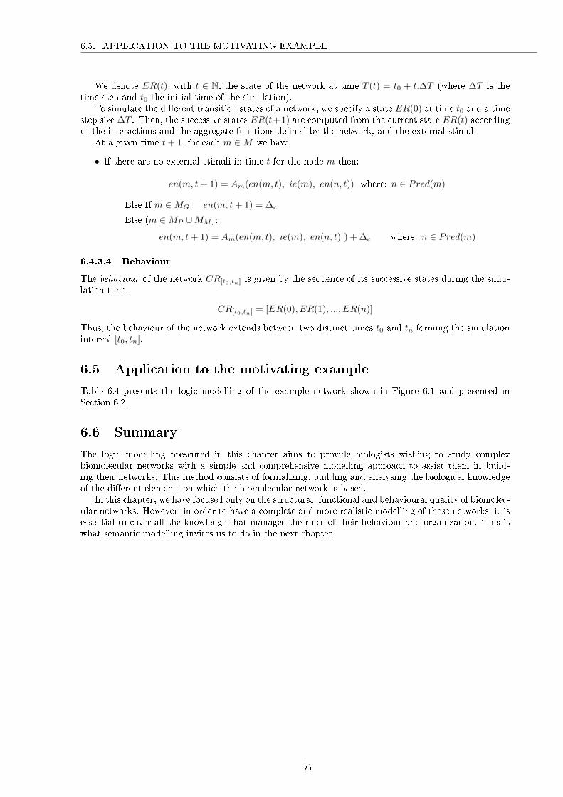
6.5. APPLICATION TO THE MOTIVATING EXAMPLE
We denote ER(t), with t ∈ N, the state of the network at time T (t) = t0 + t.∆T (where ∆T is thetime step and t0 the initial time of the simulation).
To simulate the di�erent transition states of a network, we specify a state ER(0) at time t0 and a timestep size ∆T . Then, the successive states ER(t+1) are computed from the current state ER(t) accordingto the interactions and the aggregate functions de�ned by the network, and the external stimuli.
At a given time t+ 1, for each m ∈M we have:
• If there are no external stimuli in time t for the node m then:
en(m, t+ 1) = Am(en(m, t), ie(m), en(n, t)) where: n ∈ Pred(m)
� Else If m ∈MG: en(m, t+ 1) = ∆c
� Else (m ∈MP ∪MM ):
en(m, t+ 1) = Am(en(m, t), ie(m), en(n, t) ) + ∆c where: n ∈ Pred(m)
6.4.3.4 Behaviour
The behaviour of the network CR[t0,tn] is given by the sequence of its successive states during the simu-lation time.
CR[t0,tn] = [ER(0), ER(1), ..., ER(n)]
Thus, the behaviour of the network extends between two distinct times t0 and tn forming the simulationinterval [t0, tn].
6.5 Application to the motivating example
Table 6.4 presents the logic modelling of the example network shown in Figure 6.1 and presented inSection 6.2.
6.6 Summary
The logic modelling presented in this chapter aims to provide biologists wishing to study complexbiomolecular networks with a simple and comprehensive modelling approach to assist them in build-ing their networks. This method consists of formalizing, building and analysing the biological knowledgeof the di�erent elements on which the biomolecular network is based.
In this chapter, we have focused only on the structural, functional and behavioural quality of biomolec-ular networks. However, in order to have a complete and more realistic modelling of these networks, it isessential to cover all the knowledge that manages the rules of their behaviour and organization. This iswhat semantic modelling invites us to do in the next chapter.
77
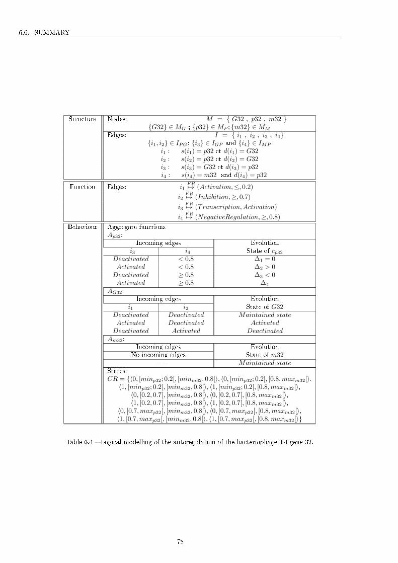
6.6. SUMMARY
Structure Nodes: M = { G32 , p32 , m32 }{G32} ∈MG ; {p32} ∈MP ; {m32} ∈MM
Edges: I = { i1 , i2 , i3 , i4}{i1, i2} ∈ IPG; {i3} ∈ IGP and {i4} ∈ IMP
i1 : s(i1) = p32 et d(i1) = G32i2 : s(i2) = p32 et d(i2) = G32i3 : s(i3) = G32 et d(i3) = p32i4 : s(i4) = m32 and d(i4) = p32
Function Edges: i1FR7→ (Activation,≤, 0.2)
i2FR7→ (Inhibition,≥, 0.7)
i3FR7→ (Transcription,Activation)
i4FR7→ (NegativeRegulation,≥, 0.8)
Behaviour Aggregate functionsAp32:
Incoming edges Evolutioni3 i4 State of cp32
Deactivated < 0.8 ∆1 = 0Activated < 0.8 ∆2 > 0Deactivated ≥ 0.8 ∆3 < 0Activated ≥ 0.8 ∆4
AG32:Incoming edges Evolution
i1 i2 State of G32Deactivated Deactivated Maintained stateActivated Deactivated ActivatedDeactivated Activated Deactivated
Am32:Incoming edges Evolution
No incoming edges State of m32� Maintained state
States:CR = {〈0, [minp32; 0.2[, [minm32, 0.8[〉, 〈0, [minp32; 0.2[, [0.8,maxm32[〉,〈1, [minp32; 0.2[, [minm32, 0.8[〉, 〈1, [minp32; 0.2[, [0.8,maxm32[〉,〈0, [0.2, 0.7[, [minm32, 0.8[〉, 〈0, [0.2, 0.7[, [0.8,maxm32[〉,〈1, [0.2, 0.7[, [minm32, 0.8[〉, 〈1, [0.2, 0.7[, [0.8,maxm32[〉,
〈0, [0.7,maxp32[, [minm32, 0.8[〉, 〈0, [0.7,maxp32[, [0.8,maxm32[〉,〈1, [0.7,maxp32[, [minm32, 0.8[〉, 〈1, [0.7,maxp32[, [0.8,maxm32[〉}
Table 6.4 � Logical modelling of the autoregulation of the bacteriophage T4 gene 32.
78
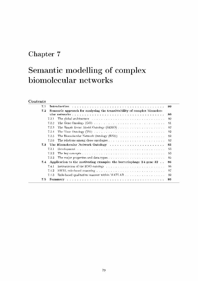
Chapter 7
Semantic modelling of complex
biomolecular networks
Contents7.1 Introduction . . . . . . . . . . . . . . . . . . . . . . . . . . . . . . . . . . . . . 80
7.2 Semantic approach for analysing the transittability of complex biomolec-
ular networks . . . . . . . . . . . . . . . . . . . . . . . . . . . . . . . . . . . . . 80
7.2.1 The global architecture . . . . . . . . . . . . . . . . . . . . . . . . . . . . . . . 80
7.2.2 The Gene Ontology (GO) . . . . . . . . . . . . . . . . . . . . . . . . . . . . . . 81
7.2.3 The Simple Event Model Ontology (SEMO) . . . . . . . . . . . . . . . . . . . . 82
7.2.4 The Time Ontology (TO) . . . . . . . . . . . . . . . . . . . . . . . . . . . . . . 82
7.2.5 The Biomolecular Network Ontology (BNO) . . . . . . . . . . . . . . . . . . . 82
7.2.6 The relations among these ontologies . . . . . . . . . . . . . . . . . . . . . . . . 82
7.3 The Biomolecular Network Ontology . . . . . . . . . . . . . . . . . . . . . . 83
7.3.1 Development . . . . . . . . . . . . . . . . . . . . . . . . . . . . . . . . . . . . . 83
7.3.2 The key concepts . . . . . . . . . . . . . . . . . . . . . . . . . . . . . . . . . . . 83
7.3.3 The major properties and data types . . . . . . . . . . . . . . . . . . . . . . . . 85
7.4 Application to the motivating example: the bacteriophage T4 gene 32 . . 86
7.4.1 Instantiation of the BNO ontology . . . . . . . . . . . . . . . . . . . . . . . . . 86
7.4.2 SWRL rule-based reasoning . . . . . . . . . . . . . . . . . . . . . . . . . . . . . 87
7.4.3 Rule-based qualitative reasoner within MATLAB . . . . . . . . . . . . . . . . . 92
7.5 Summary . . . . . . . . . . . . . . . . . . . . . . . . . . . . . . . . . . . . . . . 93
79

7.1. INTRODUCTION
7.1 Introduction
In the previous chapter, we proposed a logical-based modelling that provides the di�erent elements onwhich the biomolecular network is based. However, to obtain an optimal and more realistic modelling,we want to enhance it with an additional semantic layer. Semantic technologies, especially ontologies,are one of the tools frequently used for this purpose. In fact, they are indispensable for understandingthe semantic knowledge about the functioning of cells at a molecular level.
In this chapter, we present a semantic approach for modelling biomolecular networks and describe theproposed Biomolecular Network Ontology (BNO) created specially to address the needs of analysingthe complex biomolecular network's behaviour. This ontology provides a foundation for qualitativesimulation of these networks. The BNO ontology is freely available at https://github.com/AliAyadi/The-Biomolecular-Network-Ontology.
The �rst section of this chapter focuses on the proposed semantic approach for modelling the seman-tics of complex biomolecular networks. We detail each one of the ontologies that constitute it and therelationship among them. A second section is dedicated especially to describe in detail the main compo-nents of the BNO ontology on which the transittability of complex biomolecular networks are meant tobe contextualised. The last section presents the application of the proposed ontology through the casestudy related to the biological domain, the bacteriophage T4 gene 32 already used in Chapter 6.
7.2 Semantic approach for analysing the transittability of com-
plex biomolecular networks
Modelling the behaviour of complex biomolecular networks requires, �rst and foremost, to formalizethe domain knowledge. However, it is not su�cient to simply describe it. Certainly, the behaviourof biomolecular networks is investigated through appropriate semantic structures for the description oftheir components that must not be overlooked. Thus, the use of a formalized language such as ontologiesprovides a rich description but also allows to perform reasoning. Therefore, in this section, we proposea semantic architecture composed of four ontologies: three of them already exist in the literature, theGene Ontology (GO) [170, 329], the Simple Event Model Ontology (SEMO) [330], the Time Ontology(TO) [331] and we are developing the Biomolecular Network Ontology (BNO). Linked together, theseontologies provide the necessary concepts for modelling the dynamic behaviour and the transition statesof a complex biomolecular network. We will brie�y present the general architecture of the ontologicalprocess and describe the set of ontologies which compose our approach.
7.2.1 The global architecture
We propose a semantic approach that aims to enrich the structural description of biomolecular networks bycontextual knowledge concerning their state transitions, the events that can steer these transitions but alsotheir entire temporal context linked to this information. Thus, we present an approach for understandingthe transittability [6] of biomolecular networks which is basically composed of four ontologies: the GeneOntology (GO) [170, 329], the Simple Event Model Ontology (SEMO) [330], the Time Ontology (TO)[331] and our development, the Biomolecular Network Ontology (BNO).
Figure 7.1 describes the global architecture of our semantic approach for analysing the transittabilityof complex biomolecular networks.
This semantic architecture is based and follows the logical-based modelling of complex biomolecularnetworks detailed in Section 6.4. In fact, this correspondence between the logical and semantic mod-elling is presented in Figure 7.2. The Biomolecular Network Ontology describes the static structure ofthe biomolecular network which has already been presented in Section 6.4.1. Merging with the SimpleEvent Model Ontology, the Biomolecular Network Ontology describes what can be carried out by eachcomponent of the biomolecular network and the conditions for these activities, this notion was detailedin Section 6.4.2. Finally, the Biomolecular Network Ontology, the Simple Event Model Ontology and theTime Ontology describe how the biomolecular network and its individual components evolve over timewhich is clearly mentioned in the previous Section 6.4.3.
These ontologies are described in more detail in the sections below.
80

7.2. SEMANTIC APPROACH FOR ANALYSING THE TRANSITTABILITY OF COMPLEXBIOMOLECULAR NETWORKS
Figure 7.1 � Global architecture of our proposed semantic modelling.
Figure 7.2 � Correspondence between the logical and semantic modelling.
7.2.2 The Gene Ontology (GO)
In this study, the Gene ontology1 is considered as a core ontology. It ensures the description and theclassi�cation of cellular components. As well as, it provides a structured terminology for the descriptionof gene functions and processes, and the relationships among these components [332].
We chose to use the Gene Ontology for the following reasons, (1) it is an initiative of several genomicdatabases such as the Saccharomyces Genome Database (SGD), the Drosophila genome database (Fly-Base), etc. to build a generic ontology for describing the role of genes and proteins, (2) it is the mostdeveloped and most used in biology (since 2000), and (3) it provides annotation �les about large numberof cellular entities.
1http://www.geneontology.org
81

7.2. SEMANTIC APPROACH FOR ANALYSING THE TRANSITTABILITY OF COMPLEXBIOMOLECULAR NETWORKS
7.2.3 The Simple Event Model Ontology (SEMO)
The Simple Event Model ontology2 proposed by Van Hage et al. [330] provides the necessary knowledgefor the description of events. The ontological architecture of the Simple Event Model ontology consists offour basic concepts: Event that speci�es what is happening, Actor that indicates the participants of anevent, Place that describes the location where the event happened, and Time that describes the moment.
We chose to use the Simple Event Model ontology because it provides the necessary concepts todescribe and model events in various subject domains.
7.2.4 The Time Ontology (TO)
The Time ontology3 developed by Hobbs and Pan [331] enables a more intuitive use of the time dimensionwhile making the most of semantic knowledge. It gives a rich vocabulary to describe the topologicalrelationships that may exist between time points and intervals and also provides information about time.
The main concepts of this temporal ontology can be summarized as TemporalEntity which consistsof two sub-classes Instant and ProperInterval, DurationDescription, DateTimeDescription, TemporalU-nit, etc. Also, it contains several proprerties such as hasDurationDescription, intervalStarts, hasDate-TimeDescription, etc.
We chose to use the Time Ontology because of its basic structure that is not speci�c to a particularapplication and because it is simple to adapt it in our context.
7.2.5 The Biomolecular Network Ontology (BNO)
We developed an ontology the 'Biomolecular Network Ontology (BNO)' which aims to describe the domainknowledge of complex biomolecular networks in their static state. This ontology provides information onthe biomolecular network and its components (nodes, interactions, states, transition states, etc.) and anindication of the network's context such as the type of sub-network, the type of node, the conditions andnature of interactions, etc. This allows to precisely analyse and interpret the semantic context in orderto achieve intelligent modelling of biomolecular networks and their state changes.
The BNO ontology is the major contribution of this chapter, that is why an entire section has beendevoted to detail this ontology (Section 7.3).
7.2.6 The relations among these ontologies
Concepts in the Biomolecular Network ontology are linked to the Gene ontology concepts. In fact,the concepts of the Gene ontology are used to enrich the de�nitions of the concepts of the Biomolec-ular Network ontology by two relations: an equivalence relation owl:equivalenceClass and a speci�ca-tion relation owl:subClassOf. Some instances of these relations are shown in Figure 7.3. For example,as described in Figure 7.3a, after inference the concept BNO:Protein will be specialized by the con-cept GO:beta-galactosidase (GO: 0009341) because the BNO:Node concept is equivalent to the conceptGO:cellular_component (GO: 0005575). Other examples of these links are illustrated by Table 7.1.The Biomolecular Network ontology is also linked with the Simple Event Model Ontology through theBNO:Node concept, in fact, a SEM:event can stimulate a molecular entity (represented by the conceptBNO:Node). The Simple Event Model ontology will be used to describe the states of BNO:Node and itsbehaviour.
Moreover, the Time Ontology (TO) has been integrated into the Simple Event Model ontology. Theconcept SEM:Time was made equivalent to the concept TO:TemporalEntity which represents the rootof the Time ontology. Hence, the property SEM:hasTime will connect the Simple Event Model ontologyto the Time ontology and, as a consequence, the diverse types of temporal concepts will be de�ned asspecializations of the class SEM:Time. Figure 7.3b shows the use of this principle. Thus, we can exploitthe wealth of temporal concepts provided by this temporal ontology to describe the SEM:event class.
Using these relationships it is possible to merge these ontologies to formalize the necessary knowledgeto study the state changes of the biomolecular network's behaviour.
2http://semanticweb.cs.vu.nl/2009/11/sem/3https://www.w3.org/TR/owl-time/
82

7.3. THE BIOMOLECULAR NETWORK ONTOLOGY
(a) (b)
Figure 7.3 � Example of merging: 7.3a The Gene ontology concepts to the Biomolecular Network ontologyconcepts. 7.3b The Time ontology within the Simple Event Model ontology.
Table 7.1 � Linking of Gene Ontology concepts to the Biomolecular Network ontology.
Type of relationship Biomolecular Network Ontology concept name Gene Ontology concept name
Equivalence: BNO ′owl : equivalenceClass′ GOBNO : Node GO : cellular_componentBNO : Protein GO : protein_complex
Subclass: BNO ′owl : subClassOf ′ GO BNO : Interaction GO : biological_process
7.3 The Biomolecular Network Ontology
To study the dynamic behaviour and the transition states of biomolecular networks, it is required to modeltheir domain knowledge. Therefore, we developed the Biomolecular Network ontology. This ontologyis the major contribution of this chapter, it is intended to describe exhaustively the �eld of complexbiomolecular networks by describing the static aspect of their structure. It was de�ned in collaborationwith domain experts.
Figure 7.15 presents the Biomolecular Network ontology. We use the graphical notation for OWLontologies de�ned by Brockmans et al. [333] and Barzdin
,² et al. [334] where boxes are OWL concepts;
full lines are object properties and dotted lines are data properties. Full lines can be labelled to indicaterestrictions meaning that the range of the relationship is specialized.
7.3.1 Development
As described in Figure 7.15 and 7.4, we have developed the BNO ontology using the OWL-language[335] under the Protégé editor. Concepts, relations, and attributes were modelled as concepts, objectproperties and data properties, respectively. Axioms were represented in Protégé using diverse OWLrestrictions (existential restrictions, universal restrictions, cardinality restrictions, hasValue restrictions),characteristics of object property, and datatype restrictions.
7.3.2 The key concepts
Only a few of the object properties restrictions are displayed in Figure 7.15 for the sake of clarity. Thisdomain ontology consists of �ve main concepts:
• The Biomolecular_Network class: This class includes the di�erent types of complex biomolecularnetworks. As mentioned earlier in Section 1.4, the complex biomolecular network can be com-posed by Gene Regulatory networks (GRNs), Protein-Protein Interaction networks (PPINs) andMetabolic networks (MNs) which correspond to the following concepts: Genomic_Network, Pro-teomic_Network and Metabolomic_Network.
These types of networks can be connected to the other ontology's concepts through three properties,has_node that depicts its cellular components, has_interaction that describes the interactions
83

7.3. THE BIOMOLECULAR NETWORK ONTOLOGY
Figure 7.4 � The Biomolecular Network Ontology: hierarchy of concepts, hierarchy of properties andhierarchy of data properties.
linked to its components and the property has_node only that speci�es exactly the nature and typeof its components.
The instances of these concepts will be de�ned later, among these instances we will focus on theBacteriophageT4G32 instance in Section 7.4.1.
• The Node class: This class contains the di�erent types of cellular entities M that constitute thebiomolecular network. In fact, we can identify three sub-classes: the Gene which describes the set ofgenes MG, the set of proteins Protein which models the set MP and the Metabolite which describesthe set of metabolitesMM . The Gene sub-class is itself divided into two types the BNO : DNA andBNO : RNA. The class Node is connected with the Node_State through the property has_state.These BNO concepts are detailed on the logical-based modelling in Section 6.4.1.
• The Interaction class: This class covers all the diverse types of interactions that can be operatedamong the di�erent types of nodes of the biomolecular network. This class consists of two sub-classes, Intraomic_Interactions that covers the interactions between molecular components of thesame type and the class Interomic_Interaction that describes the interactions between molecularcomponents of the di�erent type. This class is connected to the Node class via two properties,has_source and has_end. These BNO concepts are developed through the logical-based modellingin Section 6.4.2.
• The Node_State class contains the possible states of the nodes. This class is composed of twosub-classes, the ConcentrationState and the ActivationState.
• The Interaction_Type class allows to specify the types and the nature of the interaction amongcellular components. This class is linked to the BNO:Interaction class through the propertiesHas_type.
The instances of this class belong to the set of concepts of the Interaction Ontology proposed byVan Landeghem et al. [4] (in Figure 6.4. To successfully integrate the main Interaction ontologyconcepts (IO:Activity_�ow and IO:Process) with the Biomolecular Network ontology, we create an
84

7.3. THE BIOMOLECULAR NETWORK ONTOLOGY
abstract BNO UML BNO:Interaction_Type to generalise those two Interaction ontology concepts(Figure 7.15).
Table 7.2 and Figure 7.4 show the most important BNO concepts.
Table 7.2 � A summary of concepts in the Biomolecular Network ontology. The left column presents the�ve major concepts and their immediate sub-classes. The right column presents the description of theseconcepts.
BNO ontology concepts Description
BNO:BiomolecularNetwork de�nes the di�erent kinds of complex biomolecular networks.BNO:GenomicNetwork de�nes the interactions among genes forming Gene Regulatory networks.BNO:ProteomicNetwork de�nes the interactions among proteins forming Protein-Protein Interaction networks.BNO:MetabolomicNetwork de�nes the interactions among proteins forming Metabolic networks.
BNO:Node de�nes the di�erent types of cellular entities.BNO:Gene describes the set of genes MG.BNO:DNA describes the set DNA.BNO:RNA describes the set of RNA.
BNO:Protein describes the set proteins MP .BNO:Metabolite describes the set metabolites MM .
BNO:Interaction de�nes all the types of interactions operated among the nodes.BNO:IntraomicInteraction de�nes the interactions between molecular components of the same type.BNO:I_GG de�nes the interactions between genes.BNO:I_PP de�nes the interactions between proteins.BNO:I_MM de�nes the interactions between metabolites.
BNO:InteromicInteraction de�nes the interactions between molecular components of the di�erent type.BNO:I_GP de�nes the interactions between genes and proteins.BNO:I_PG de�nes the interactions between proteins and genes.BNO:I_PM de�nes the interactions between proteins and metabolites.BNO:I_MP de�nes the interactions between metabolites and proteins.
BNO:NodeState de�nes the possible states of the nodes.BNO:ActivationState de�nes the states of the genes.BNO:ConcentrationState de�nes the concentration of the proteins and metabolites.
BNO:InteractionType de�nes the nature of the interaction among cellular components.
7.3.3 The major properties and data types
After the de�nition of the major concepts of the BNO ontology and in order to describe the semanticrelations among them, we de�ne the domain, range, property type and inverse properties as constraintconditions. The di�erent properties and data types of the BNO ontology are explained below.
• hasBehaviour(object1, object2): where object1 is aBiomolecularNetwork and object2 is aBehaviour.
• hasInteraction(object1, object2): where object1 is a BiomolecularNetwork and object2 is anInteraction.
• hasNode(object1, object2): where object1 is a BiomolecularNetwork and object2 is a Node.
• hasSource(object1, object2): where object1 is an Interaction and object2 is a Node.
• hasEnd(object1, object2): where object1 is an Interaction and object2 is a Node.
• hasState(object1, object2): where object1 is a Node and object2 is a NodeState.
• hasTypeInteraction(object1, object2): where object is an Interaction and object2 is a TypeInteraction.
• deltaC(object, dc): where object is an Interaction and dc is a float representing the change inconcentration caused by the interaction.
• forT ime(object, t): where object is a NodeState and t is a int representing its time.
• hasConcentrationV alue(object, c): where object is a Protein or a Metabolite and c is a floatrepresenting the value of its concentration.
85

7.4. APPLICATION TO THE MOTIVATING EXAMPLE: THE BACTERIOPHAGE T4 GENE 32
• isActivated(object, bv): where object is an Gene and bv is a boolean equal to true if the gene isactivated.
• threshold(object, t′): where object is the threshold of an Interaction and t
′a comparison operator
(≤ or ≥) determining the minimum and maximum threshold, respectively.
Table 7.3 summarises the major properties of the BNO ontology, including their domain, range andinverse.
Table 7.3 � A summary of the properties, including their domain, range and inverse.
BNO ontology properties Domain Range InversehasBehaviour BiomolecularNetwork Behaviour isBehaviourOfhasInteraction BiomolecularNetwork Interaction isInteractionOf
hasNode BiomolecularNetwork Node isNodeOfhasSource BiomolecularNetwork Node isSourceOfhasEnd Interaction Node isEndOfhasState Interaction State isStateOf
hasTypeInteraction Interaction TypeInteraction isTypeInteractionOf
7.4 Application to the motivating example: the bacteriophage
T4 gene 32
Figure 7.5 � Instantiation of the BNO ontology for the given example.
The aim of this section is to illustrate the proposed BNO ontology for reasoning and inferring newknowledge with sets of rules expressed in SWRL [335]. To do this, we test its performance by using thereal example presented in Section 6.2, the bacteriophage T4 gene 32.
7.4.1 Instantiation of the BNO ontology
Figure 7.5 presents the instantiation of the BNO ontology for the given example of the bacteriophage T4gene 32. The BNO ontology provides detailed and rigorous semantics to model this biomolecular network.
86

7.4. APPLICATION TO THE MOTIVATING EXAMPLE: THE BACTERIOPHAGE T4 GENE 32
We use the Protégé editor to instantiate the BNO ontology for the bacteriophage T4 gene 32. Figure7.6 illustrates the nodes instantiations respectively, the gene G32, protein p32 and metabolite m32. Theinstantiations of the four reactions are detailed in Figure 7.7.
Figure 7.6 � A snapshot look at the BNO node instances associated with the given example displayingrespectively: (1) the gene G32, (2) the protein p32 and (3) the metabolite m32.
Figure 7.7 � A snapshot look at the BNO interaction instances associated with the given example dis-playing respectively: (1) Activation, (2) Inhibition, (3) Transcription and (4) Catalysis.
7.4.2 SWRL rule-based reasoning
As detailed in Section 3.6.1, the Semantic Web Rule Language (SWRL) is an ontological language basedon OWL-DL and OWL-Lite that expresses the rule description language based on OWL [336]. SWRL canbe used to write rules to reason about OWL individuals and infer new knowledge about those individuals.The rules in SWRL are implication rules, and follow this syntax: antecedent → consequent. This formmeans that the consequent must be true when the antecedent is satis�ed. In SWRL rules, the symbol '∧'means conjunction, '?x' is a variable, '→' means implication. A symbol without the leading '?' denotesthe name of an instance (an individual) in the ontology. These SWRL rules can provide additionalexpressiveness to OWL-based ontologies. Thus we adopt these SWRL rules to build the reasoning rules
87

7.4. APPLICATION TO THE MOTIVATING EXAMPLE: THE BACTERIOPHAGE T4 GENE 32
in order to represent the dynamic aspect of the biomolecular network. During this reasoning, inferencesare made, classifying the instances of the BNO ontology and associating new properties to create instanceswhile maintaining logical consistency.
7.4.2.1 Inhibition SWRL rule
The following rule models the inhibition interaction. When the concentration of the protein p32 exceedsthe threshold 0.7 10−6 Mol/L−1, it inhibits the translation of its gene G32.
ADN(?g) ∧ hasState(?g, ?gs1) ∧ forTime(?gs1, ?t) ∧ hasState(?g, ?gs2) ∧ forTime(?gs2,?t2) ∧ swrlb:add(?t2, ?t, 1) ∧ Protein(?p) ∧ Activation(?activ) ∧ hasSource(?activ, ?p) ∧hasEnd(?activ, ?g) ∧ hasState(?p, ?ps) ∧ forTime(?ps, ?t) ∧ hasConcentrationValue(?ps,?c) ∧ swrlb:greaterThanOrEqual(?c, 0.7) → isActivated(?gs2, false)
As depicted in Figure 7.8, the results of this rule means that, If there is a gene g having a state gs equalto true at a given time t and there is a protein p having a state ps1 and a concentration c at this timet, and these two molecules g and p are related by an Inhibition interaction, and if the concentration of pexceeds a threshold equal to 0.7, then the state of g move to false at time t+ 1.
Figure 7.8 � Results of the reasoning process for the Inhibition SWRL rule.
7.4.2.2 Activation SWRL rule
In contrast to the �rst rule, this rule models the activation interaction. When the concentration of theprotein p32 becomes less than the threshold 0.2 10−6 Mol/L−1, it activates the translation of the geneG32.
ADN(?g) ∧ hasState(?g, ?gs1) ∧ forTime(?gs1, ?t) ∧ hasState(?g, ?gs2) ∧ forTime(?gs2,?t2) ∧ swrlb:add(?t2, ?t, 1) ∧ Protein(?p) ∧ Activation(?activ) ∧ hasSource(?activ, ?p) ∧hasEnd(?activ, ?g) ∧ hasState(?p, ?ps) ∧ forTime(?ps, ?t) ∧ hasConcentrationValue(?ps,?c) ∧ swrlb:lessThanOrEqual(?c, 0.2) → isActivated(?gs2, true)
88

7.4. APPLICATION TO THE MOTIVATING EXAMPLE: THE BACTERIOPHAGE T4 GENE 32
As described in Figure 7.9, the results of this rule means that, If there is a gene g having a state gs equalto false at a given time t and there is a protein p having a state ps1 and a concentration c at this time t,and these two molecules g and p are related by an Activation interaction, and if the concentration of p isunder a threshold equal to 0.2, then the state of g move to true at time t+ 1.
Figure 7.9 � Results of the reasoning process for the Activation SWRL rule.
7.4.2.3 Transcription SWRL rule
The following rule represents the gene transcription. In fact, if the gene G32 is activated, this onegenerates the protein synthesis and produces an increase in the concentration of this protein p32.
ADN(?g) ∧ hasState(?g, ?gs) ∧ forTime(?gs, ?t) ∧ isActivated(?gs, true) ∧ Protein(?p)∧ Transcription(?trans) ∧ hasSource(?trans, ?g) ∧ hasEnd(?trans, ?p) ∧ hasState(?p,?ps1) ∧ forTime(?ps1, ?t) ∧ hasConcentrationValue(?ps1, ?c1) ∧ hasState(?p, ?ps2) ∧forTime(?ps2, ?t2) ∧ swrlb:add(?t2, ?t, 1) → hasConcentrationValue(?ps2, ?c2)
The result of this rule is interpreted as (Figure 7.10), If there is a gene g having a state gs equal to true ata given time t and there is a protein p having a state ps1 and a concentration c at this time t, and thesetwo molecules g and p are related by a Transcription interaction, then the concentration of the protein pincreases at time t+ 1. In the opposite case, we have this rule:
ADN(?g) ∧ hasState(?g, ?gs) ∧ forTime(?gs, ?t) ∧ isActivated(?gs, false) ∧ Protein(?p)∧ Transcription(?trans) ∧ hasSource(?trans, ?g) ∧ hasEnd(?trans, ?p) ∧ hasState(?p,?ps1) ∧ forTime(?ps1, ?t) ∧ hasConcentrationValue(?ps1, ?c1) ∧ hasState(?p, ?ps2) ∧forTime(?ps2, ?t2) ∧ swrlb:add(?t2, ?t, 1) → hasConcentrationValue(?ps2, ?c1)
The result of this rule means that (Figure 7.11), If there is a gene g having a state gs equal to false at agiven time t and there is a protein p having a state ps1 and a concentration c at this time t, and thesetwo molecules g and p are related by a Transcription interaction, then the concentration of the protein premains stable at time t+ 1.
Results of the Transcription SWRL rule and its opposite rule are presented in Figure 7.10 and Figure7.11, respectively.
89

7.4. APPLICATION TO THE MOTIVATING EXAMPLE: THE BACTERIOPHAGE T4 GENE 32
Figure 7.10 � Results of the reasoning process for the Transcription SWRL rule.
Figure 7.11 � Results of the reasoning process for the inverse of Transcription SWRL rule.
90

7.4. APPLICATION TO THE MOTIVATING EXAMPLE: THE BACTERIOPHAGE T4 GENE 32
7.4.2.4 Negative regulation SWRL rule
As well, following the increase of the concentration of the protein p32, a negative regulation interactionresulted to create hormone balance. This reaction is ensured by the following rule:
Metabolite(?m) ∧ hasState(?m, ?ms) ∧ hasConcentrationValue(?ms, ?c) ∧ forTime(?ms,?t) ∧ Protein(?p) ∧ Negative_regulation(?negreg) ∧ hasSource(?negreg, ?m) ∧ hasEnd(?negreg,?p) ∧ deltaC(?negreg, ?delta) ∧ hasState(?p, ?ps1) ∧ forTime(?ps1, ?t) ∧ hasConcentra-tionValue(?ps1, ?c1) ∧ hasState(?p, ?ps2) ∧ forTime(?ps2, ?t2) ∧ swrlb:add(?t2, ?t, 1)∧ swrlb:greaterThanOrEqual(?c, 0.8) ∧ swrlb:subtract(?c2, ?c1, ?delta) → hasConcentra-tionValue(?ps2, ?c2)
The meaning of this rule is (Figure 7.12), If there is a metabolite m having a state ms associated to aconcentration value c at a given time t and there is a protein p having a state ps1 and a concentrationc1 at this time t, and these two molecules m and p are related by a negative regulation interaction, and ifthe concentration of m exceeds a threshold equal to 0.8, then the concentration of the protein p decreasesat time t+ 1.
In contrast, when the concentration of the metabolite m32 is less than 0.8 we applied the followingrule:
Metabolite(?m) ∧ hasState(?m, ?ms) ∧ hasConcentrationValue(?ms, ?c) ∧ forTime(?ms,?t) ∧ Protein(?p) ∧ Negative_regulation(?negreg) ∧ hasSource(?negreg, ?m) ∧ hasEnd(?negreg,?p) ∧ deltaC(?negreg, ?delta) ∧ hasState(?p, ?ps1) ∧ forTime(?ps1, ?t) ∧ hasConcentra-tionValue(?ps1, ?c1) ∧ hasState(?p, ?ps2) ∧ forTime(?ps2, ?t2) ∧ swrlb:add(?t2, ?t, 1)∧ swrlb:lessThan(?c, 0.8) → hasConcentrationValue(?ps2, ?c1)
Figure 7.12 � Results of the reasoning process for the Negative regulation SWRL rule.
Which means (Figure 7.13), If there is a metabolite m having a state ms associated to a concentrationvalue c at a given time t and there is a protein p having a state ps1 and a concentration c1 at this time t,and these two molecules m and p are related by a negative regulation interaction, and if the concentrationof m is under a threshold equal to 0.8, then the concentration of the protein p remains stable at time
91

7.4. APPLICATION TO THE MOTIVATING EXAMPLE: THE BACTERIOPHAGE T4 GENE 32
Figure 7.13 � Results of the reasoning process for the inverse of the Negative regulation SWRL rule.
t + 1. Results of the Negative regulation SWRL rule and its opposite rule are presented in Figure 7.12and Figure 7.13, respectively.
To conclude, the case study with OWL-SWRL rules represents a �proof of concept� since it demon-strates the logical consistency of the BNO ontology and validates its relevance. To check the inconsis-tencies and violations of these SWRL rules, we used the latest version of HermiT reasoning plugin inthe Protégé 5 environment4 version 1.3.8.3. Obtained results prove that the BNO ontology is consis-tent, credible and e�ective in describing relevant knowledge required in understanding the behaviour ofcomplex biomolecular networks and their state changes. However, we must emphasise that, even if thisontology provides useful knowledge and rich semantics allowing biologists to understand the dynamicalbehaviour of complex biomolecular networks, it can not simulate large-scale networks. That is why moree�cient simulation tools should be used for scaling up and reason on large biomolecular networks.
7.4.3 Rule-based qualitative reasoner within MATLAB
Despite the SWRL rule-based reasoning, extensive experiments were conducted to validate our proposedontology including the implementation of the rule-based qualitative reasoner. This rule-based reasoneris implemented under the MATLAB development environment and can be freely downloaded at https://github.com/AliAyadi/Qualitative\ReasoningInMATLAB. The reasoner is based on a qualitativesimulation algorithm 1, with speci�c reference to the SWRL rules de�ned in the previous Section 7.4.2.
Algorithm 1 provides a high-level description of the general reasoning algorithm of a complex biomolec-ular network. The main steps of this algorithm are: (1) The de�nition of the set of SWRL rules andtheir thresholds. (2) The initialization time and the state of all molecular components; (3) Evaluate thenode state; (4) Launch the speci�c reaction de�ned by the corresponding SWRL rule when the node statereached a threshold; and (5) Update the novel value of the state node.
Figure 7.14 depicts the individual qualitative behaviour of the biomolecular components. Indeed,for each node, a description of its dynamical time-evolution is graphically presented. The evolution is
4http://www.hermit-reasoner.com/
92

7.5. SUMMARY
Algorithm 1 Pseudocode of the qualitative simulation algorithm
1: De�nition of the set of SWRL rules and their thresholds.2:
3: Initialization of time and network's state.4: for All time step from begining to end_of_simulation do5: for Each molecular component do6: Evaluate the node state7: if the component's state achieves one threshold then8: Execution of the reaction de�ned by the SWRL rule corresponding to this threshold.9: . Measure the state if it is a gene and the concentration if it is a protein or a metabolite10: Update the novel state of the node.11: end if12: end for13: end for
displayed as a graph to easily see when and how the molecular component evolves during the simulationand to precisely detect changes in the state in time. These results are not di�cult to interpret, becauseat each simulation step a qualitatively meaningful network state is reached. The results are close tohuman reasoning. In fact, this qualitative reasoning is based on the SWRL rules presented above whichrepresent a set of constraints equations describing the relevant structural and functional relationships inthe biomolecular network. The possible behaviours and states of the network may be predicted fromthese constraints rules and an initial state. The behavioural description of the biomolecular network andits individual components may be used to explain a set of hypothesis and determine the change directionsof the network behaviour.
Figure 7.14 � Simulation results plotted with the MATLAB environment: the individual qualitativebehaviour of the biomolecular components.
7.5 Summary
This chapter proposes an e�ective approach for analysis and understanding the behaviour of complexbiomolecular networks over time. The use of a semantic approach based on merging di�erent ontologies
93

7.5. SUMMARY
can overcome issues of study the state changes of complex biomolecular networks and their behaviour.Indeed, we developed the Biomolecular Network Ontology (BNO) to describe the static structure ofcomplex biomolecular networks and merge it with the Gene Ontology (GO) to provide structured ter-minologies for the description of cellular components. We also chose the Simple Event Model Ontology(SEMO) to describe events and stimuli which can stimulate the network's components and integrate theTime Ontology (TO) to study the di�erent states of the biomolecular network and its nodes over time.
The Biomolecular Network Ontology developed in this chapter aims to describe the domain knowl-edge of complex biomolecular networks in their static state. This ontology provides information on thebiomolecular network and its components (nodes, interactions, states, transition states, etc.) and anindication of the network's context such as the type of sub-network, the type of node, the conditions andnature of interactions, etc. This allows to precisely analyse and interpret the semantic context in orderto achieve intelligent modelling of biomolecular networks and their state changes. These state changescan be computed with a rule-based system.
The SWRL rule-based reasoning and rule-based qualitative reasoner within MATLAB have beenused to validate the BNO ontology and to demonstrate how it is capable of providing useful knowledgeand rich semantics allowing biologists to understand and simulate the dynamical behaviour of complexbiomolecular networks. However, the BNO ontology can not simulate large-scale networks. That is whymore e�cient simulation tools should be used for scaling up and reason on large biomolecular networks,this is the topic of the next chapter.
94

7.5. SUMMARY
Figure 7.15 � The Biomolecular Network Ontology (BNO).
95

7.5. SUMMARY
96

Chapter 8
Qualitative, discrete-event simulation
simulation of complex biomolecular
networks
Contents8.1 Introduction . . . . . . . . . . . . . . . . . . . . . . . . . . . . . . . . . . . . . 98
8.2 Qualitative simulation model . . . . . . . . . . . . . . . . . . . . . . . . . . . 98
8.2.1 Qualitative reasoning . . . . . . . . . . . . . . . . . . . . . . . . . . . . . . . . 98
8.2.2 Basic concepts . . . . . . . . . . . . . . . . . . . . . . . . . . . . . . . . . . . . 98
8.2.3 Application to the motivating example: the bacteriophage T4 gene 32 . . . . . 100
8.3 Discrete-event simulation model . . . . . . . . . . . . . . . . . . . . . . . . . 103
8.3.1 Mapping the logical based modelling with the DEVS formalism . . . . . . . . . 103
8.3.2 Discrete-event simulation algorithm . . . . . . . . . . . . . . . . . . . . . . . . 103
8.3.3 Application to the motivating example: the bacteriophage T4 gene 32 . . . . . 105
8.4 Summary . . . . . . . . . . . . . . . . . . . . . . . . . . . . . . . . . . . . . . . 107
97

8.1. INTRODUCTION
8.1 Introduction
The complexity of biomolecular networks is �rstly due to their large number of coupled components,but also to the diversity of these molecular components and to their intricate interactions. Indeed,biomolecular networks consist of various subnetworks which themselves are composed of several molecularcomponents interacting in turn with each other, producing a complex global behaviour. The complexityand large size of these networks have prevented a fully quantitative simulation. Thus, biologists requiretools allowing them to gain insights into the behaviour of complex biomolecular networks by simulatingthe di�erent states of their components over time.
In this chapter, we propose two kinds of simulation: a qualitative and a discrete-event simulation.The �rst one responds to the complexity of calculating the quantitative reasoning methods which some-times are impossible to implement. Then, the second method is an integrative discrete-event simulationconsidering that the behaviour of the complex biomolecular network emerges from the network-levelinteraction.
The �rst section of this chapter presents the qualitative simulation method and detail all its construc-tion steps. Then, the second section of this chapter presents a discrete-event simulation approach that isable to reproduce the behaviour of complex biomolecular networks and their components over time. Thissimulation is based on the combination of the logical-based modelling of complex biomolecular networks(which is presented in Chapter 6) and a discrete-event simulation algorithm inspired by the discrete-event system speci�cation formalism (detailed in Section 4.3.4). Moreover, we enrich and explain thesesimulation methods by applying them with the case study of the bacteriophage T4 gene 32.
8.2 Qualitative simulation model
In our works, the explicit representation of the network behaviour evolution, between two instants t0 andtn is essential. Therefore, we must link the logical-based modelling de�ned in Chapter 6 to a qualitativesimulation mechanism. This simulation allows executing the model in order to simulate the networkevolution and its components over time.
8.2.1 Qualitative reasoning
The reasoning is a mental activity that humans practice to solve di�culties they confront in their life.This reasoning is often performed in the lack of quantitative knowledge and is then called qualitativereasoning. In literature, we distinguish two types of reasoning, heuristic reasoning which is a mentalshortcut and causal reasoning which is based on a model [8]. The second case of reasoning is based onthe modelling of the system. Such reasoning is based on a model of causal type because it combines thee�ects and causes, such as a causal graph. It solves a problem by reasoning about the structure andfunction of the object in an application environment and their behaviour over time [337, 338].
We chose to use qualitative reasoning for two reasons: (1) To understand the overall functioning andproperties of complex biomolecular networks through the analysis and simulation of the dynamical model(explained in the previous section), and the interpretation of the obtained knowledge. (2) To steer thesenetworks by allowing to evaluate their simulation at any time.
8.2.2 Basic concepts
In the following sections, we will de�ne the basic concepts of qualitative simulation [8] and detail themajor phases of construction.
8.2.2.1 The causal graph
The qualitative simulation model is based on the development of a causal graph whose nodes denotevariables that are related to this simulation and edges denote causality relations among these variables. Byanalogy with the logical-base modelling presented in Chapter 6, the causal graph is itself the biomolecularnetwork SR where its nodes represent causal states of network's molecular components and its edgesrepresent the types of interactions that can occur among these components.
98

8.2. QUALITATIVE SIMULATION MODEL
8.2.2.2 Quantitative variables & Quantity space
A variable is a characteristic of interest. For example, in our case the variables of the qualitative modeldenote the state of the molecular components at a given moment denoted by en(m, t). Thesevariables are qualitative because they are represented by qualities (nominal or ordinal).
The set of these qualitative values and their corresponding intervals constitutes the quantity spaceof the variable en(m, t), denoted by EQen(m,t). Each variable en(m, t) takes its qualitative value in itsordered set of qualitative values EQen(m,t) = {vq1, vq2, ..., vqn}. In fact, the quantity space is a partitionof the domain of a variable values into behaviour regions that are qualitatively homogeneous.
As de�ned in Algorithm 2, the partition of the quantity space EQen(m,t) depends on the type of node:
• If m ∈ MG : en(m, t) = {Deactivated,Activated}, its states can be 'Activated ' or 'Deactivated '.So, we assign to its EQen(m,t) the qualitative values 0 and 1 meaning respectively 'Deactivated ' and'Activated '.
en(m, t) = {Deactivated,Activated}⇒ EQen(m,t) = {0, 1}
• If m ∈ MP ∪MM : EQen(m,t) depends on the outgoing arcs oe(m) starting from the node m. Infact, as illustrated in Figure 8.1 for a quantity n of outgoing arcs, there will be n + 1 qualitativevalues that are de�ned by an order relation on EQen(m,t), creating an ordered set of qualitativevalues EQen(m,t) = {vq1, vq2, ..., vqn}.
en(m, t) = {[minm, Threshold1[, [Threshold1, Threshold2[, ..., [Thresholdn,maxm]}⇒ EQen(m,t) = {vq1, vq2, ..., vqn}
To resolve the con�icts of partitioning the EQen(m,t), we present the following algorithm.
Algorithm 2 Pseudocode of the EQen(m,t) partitioning algorithm
Require: m ∈M , oe(m), minm, maxm, EQen(m,t) ← ∅Ensure: Partition of EQen(m,t)
1: if (m ∈MP ∪MM ) then2: for outgoing edges i ∈ oe(m) do3: Read its Threshold;4: Sort the threshold values;
Threshold1 < Threshold2 <, ..., < Thresholdn
5: Quantitative partitioning of EQen(m,t);
EQen(m,t) = {[minm;Threshold1], [Threshold1, Threshold2], ..., [Thresholdn,maxm]}6: Translate quantitative measures into qualitative values;
EQen(m,t) = {vq1, vq2, ..., vqn+1}Where: vq1 = [minm, Threshold1] and ||EQen(m,t)|| = ||oe(m)||+ 1
7: end for
8: Return the quantity space
EQen(m,t) = {vq1, vq2, ..., vqn+1}9: else
10: if (m ∈MG) then11: Boolean partitioning of EQen(m,t);
EQen(m,t) = {true, false}12: Translate boolean measures into qualitative values;
EQen(m,t) = {vq1, vq2}Where: vq1 = 0, vq2 = 1 and ||EQen(m,t)|| = 2
13: Return the quantity space
EQen(m,t) = {vq1, vq2}14: end if
15: end if
Figure 8.1 displays the execution of the EQen(m,t) partitioning algorithm in both cases. In addition
99

8.2. QUALITATIVE SIMULATION MODEL
Figure 8.1 � Description of the EQen(m,t) partitioning algorithm.
to the quantity space of its variables, a qualitative reasoning method also includes algebraic relations(constraints, in�uences, etc.) that act among these quantity space.
8.2.2.3 Operations and rules
The operations In [8], the authors de�ne six operations for calculating the quantity spaces of thevariables. Among them, we will just use the three unary operations shown in Table 8.1: the incrementation(incr), the decrementation (decr) and the inverse (inv) of a qualitative variable vqi.
Using these operators, we can combine several variables together to create our own operations as aspeci�c combination table.
The partition and propagation rules Based on the work presented in [8], we adapt a qualitativereasoning mechanism to compute the qualitative value of the nodes. As shown in Figure 8.2, this mecha-nism is based on both the partition rules and the propagation rules. These rules are used to compute thevalue of the target variable (en(m, t+ 1)) at the next time t+ 1 based on its qualitative value (en(m, t))and the value of its predecessors (en(Pred(m), t)) at the current time t.
• Partition rules allow the translation of quantitative measures of the variables (en(m, t)) into qual-itative values. They match a quantitative (real) interval with its corresponding qualitative valuebelonging to the quantity space EQen(m,t). They are de�ned by the pseudo code of the algorithm2.
• Propagation rules compute the propagation of the qualitative values from the source componentsto the target components of the causal graph. They are de�ned by the aggregate functions Amwhich compute the evolution of the node status between two successive instants of the simulation(this function is detailed in Section 6.4.3). These rules are expressed by combining the operationspresented in Table 8.1.
8.2.3 Application to the motivating example: the bacteriophage T4 gene 32
In order to demonstrate the di�erent notions of this qualitative mechanism and to test its performance,we apply it to the example of the bacteriophage T4 gene 32 detailed in Section 6.2.
100

8.2. QUALITATIVE SIMULATION MODEL
Operations on EQUnary operations∀[en(m, t)] ∈ EQen(m,t) = {vq1, vq2, vq3, vq4, vq5}and n ∈ N
Incrementation 'incr'incr0([m]) = [en(m, t)][en(m, t)] : vq1 vq2 vq3 vq4 vq5- - - - - - - - - - - - - - - - - - - - - - - - - - - - - - -incr1([en(m, t)]) : vq2 vq3 vq4 vq5 vq5incrn([en(m, t)]) = incrn−1(incr1([en(m, t)]))
Decrementation 'decr'decr0([en(m, t)]) = [en(m, t)][en(m, t)] : vq1 vq2 vq3 vq4 vq5- - - - - - - - - - - - - - - - - - - - - - - - - - - - - - - -decr1([en(m, t)]) : vq1 vq1 vq2 vq3 vq4decrn([en(m, t)]) = decrn−1(decr1([en(m, t)]))
Inverse 'inv'[en(m, t)] : vq1 vq2 vq3 vq4 vq5- - - - - - - - - - - - - - - - - - - - - - - - - - - - -inv([en(m, t)]) : vq5 vq4 vq3 vq2 vq1
Table 8.1 � Unary operations on quantity spaces presented in [8].
Figure 8.2 � Qualitative reasoning mechanism.
8.2.3.1 The variables
In the example presented in Figure 6.1, we have three variables en(G32, t), en(p32, t) and en(m32, t) thatrespectively represent the state of the gene G32, the protein p32 and the metabolite m32.
8.2.3.2 The causal graph
We can use the structure of the biomolecular network as the causal graph of our example. This structureis de�ned in more details in Section 6.4.1.
8.2.3.3 The partition rules
en(G32, t) ∈ {Deactivated , Activated},⇒ EQen(G32,t) = {0 , 1}.
en(p32, t) ∈ {[minp32, 0.2[ , [0.2, 0.7[ , [0.7,maxp32[},⇒ EQen(p32,t) = {vq1 , vq2 , vq3}.
en(m32, t) ∈ {[minm32, 0.8[ , [0.8,maxm32[},⇒ EQen(m32,t) = {vq1 , vq2}.
101

8.2. QUALITATIVE SIMULATION MODEL
8.2.3.4 The propagation rules
For reasons of clarity, we note [m]t the qualitative value of the state of the component m at time t. Itmeans that the notation [m]t ≡ [en(m, t)] ∈ EQen(m,t). Now, let us de�ne the aggregate rules of eachvariables.For the variable G32:
[G32]t+1 = AG32([G32]t, {i1, i2}, [p32]t) :
if ([p32]t = vq1) then
[G32]t+1 = 1
else if ([p32]t = vq2) then
[G32]t+1 = [G32]t
else if ([p32]t = vq3) then
[G32]t+1 = 0
For the variable p32:
[p32]t+1 = Ap32([p32]t, {i3, i4}, [G32]t, [m32]t) :
if ([m32]t = vq1) ∧ ([G32]t = 0) then
[p32]t+1 = [p32]t
else if ([m32]t = vq2) ∧ ([G32]t = 0) then
[p32]t+1 = decr([p32]t)
else if ([m32]t = vq1) ∧ ([G32]t = 1) then
[p32]t+1 = incr([p32]t)
else if ([m32]t = vq2) ∧ ([G32]t = 1) then
[p32]t+1 = [p32]t
For the variable M32:
[m32]t+1 = Am32([m32]t)
⇒ [m32]t+1 = [m32]t
8.2.3.5 The simulation
Let us de�ne the initial state of the network at t0: ER(t0) = 〈[G32]t0 , [p32]t0 , [m32]t0〉.We chose the initial qualitative values of the components as: ER(t0) = 〈0, vq1, vq1〉.Then, we have performed a series of simulations to assess the evolution of the network over time:
ER(t0 + 1) = 〈[G32]t0+1, [p32]t0+1, [m32]t0+1}= 〈1, vq1, vq1〉
ER(t0 + 2) = 〈[G32](t0+1)+1, [p32](t0+1)+1, [m32](t0+1)+1〉= 〈1, vq2, vq1〉
8.2.3.6 The behaviour
CR[t0,t2] = {ER(0), ER(1), ER(2)}= {〈0, vq1, vq1〉, 〈1, vq1, vq1〉, 〈1, vq2, vq1〉}
Figure 8.3 presents the possible states of each molecular components during the simulation. This is thequalitative simulation of the given example according to the possible initial states of the components.The possible molecular states presented in this Figure referred to the set of the network states presentedin the last column of Table 6.4.
102

8.3. DISCRETE-EVENT SIMULATION MODEL
Figure 8.3 � All possible simulation results of our example.
8.3 Discrete-event simulation model
In this section, we present an approach for simulating the behaviour of complex biomolecular networksinspired by the DEVS formalism [339] detailed in Section 4.3.4, a formalism for supporting the modellingof complex systems.
8.3.1 Mapping the logical based modelling with the DEVS formalism
Before proposing our discrete-event algorithm, it is necessary to link the di�erent parts of the logicalmodelling with their corresponding notions of the DEVS formalism. As discussed in Section 6.4, thelogical-based modelling is based on three basic modelling pillars: (1) The structural modelling SR, todescribe the architecture of the biomolecular network. (2) The functional modelling FR, to describewhat can carry out each component of the biomolecular network, specifying the conditions for theseactivities. (3) And the behavioural modelling CR[t0,tn], to describe how the biomolecular networkand its individual components evolve during the simulation period [t0, tn]. Therefore, the biomolecularnetwork BN is de�ned as: BN = (SR,FR,CR[t0,tn]).
We follow this tripartite classi�cation to make the mapping between the logical-based modelling andthe DEVS formalism. The structure of the biomolecular network SR (Section 6.4.1) is composed by the setof nodesM which corresponds to the set of DEVS componentsD, and the set of interactions I correspondsto the set of the internal links among DEVS components IC. The function of the biomolecular network,represented by the function FR, corresponds to the internal transition function δint. In the logical-basedmodelling, the behaviour of complex biomolecular networks is represented with multiple parameters. The�rst parameter consists of the function en(m, t) that de�nes the state of each component, and the functionER(t) that de�nes the state of the network at time t. These functions correspond to the set of DEVScomponents S in the DEVS formalism. The aggregate function Am corresponds to a set of functions inDEVS formalism which consists of the internal transition function δint, the external transition functionδext, the con�uent transition function δcon and the time advance function ta. The external stimulirepresented by S corresponds in DEVS formalism to the set X of input events. Finally, the behaviour ofthe network CR[t0,tn] corresponds in DEVS formalism to the set Y of output events which represent theevolution of each DEVS component during the period of simulation.
8.3.2 Discrete-event simulation algorithm
In this section, we describe the basic model of the proposed discrete-event simulation algorithm, withspeci�c reference to the logical-based modelling developed in Chapter 6) and following the approachpresented in Zeigler et al. [339] (detailed in Section 4.3.4). Algorithm 6 provides a high-level description
103

8.3. DISCRETE-EVENT SIMULATION MODEL
of the general simulator algorithm of a complex biomolecular network. The main steps of this algorithmare: (1) The initialization time and the state of all molecular components; (2) The execution of theaggregate function to compute the evolution of the node in the next iteration; (3) Evaluate the nodestate; (4) Launch the speci�c reaction if the node state reached a threshold; and (5) Update the value ofthe node.
Algorithm 3 Pseudocode of the general simulator algorithm
1: Initialization: t0, ER(t0) . Initialisation of time and network's state.2: for All time step t from begining to end_of_simulation do3: for Each component mi ∈M do4: Execution of the aggregate function Ami . Launch the aggregate function manages the
evolution of the node mi
5: (Value, Threshold) = TestState(en(mi, t), FR(mi)) . Evaluate the node state6: if Value = true then . If the state of a node state achieves a threshold7: LaunchReaction(FR(en(mi, t))) . Launch the reaction de�ned by the function FR8: Update the node's state (en(mi, t)) . Update the novel state of the node9: end if10: end for11: end for
At the beginning of the simulation, the simulator initialises the network's state ER(0) = 〈en(m1, 0),en(m2, 0), ..., en(mn, 0)〉, and time t = 0.
After each iteration, the simulator evaluates the state of each node. This step is done by the TestStatefunction 4. This function requires the speci�cation of two parameters: the state of the node mi at thistime t which is provided by the function en(mi, t) (see Section 6.4.3) and its function FR(mi). Thisfunction compares the value of the state with the set of Thresholds de�ned by its function FR. If thevalue of en(mi, t) reached a threshold, it returns a boolean value equal to true and the reached threshold,else it returns the boolean value false.
Algorithm 4 Pseudocode of the TestState function
function TestState(en(mi, t), FR(mi))2: for Each Threshold ∈ ae(mi) do . Compare the state of the molecule mi with all thresholds
if en(mi, t) reached Threshold then4: return (true, Threshold); . If a threshold is reached it returns true and the reached
thresholdelse
6: return (false, �);end if
8: end forend function
Once the comparison has been done and according to the result returned by the TestState function,the simulator runs the LaunchReaction procedure de�ned by Algorithm 5. This procedure requires thespeci�cation of two parameters: the Threshold returned by the TestState function and the functionFR(mi). According to these two parameters, the procedure launch the speci�c reaction correspondingto the type of the interaction de�ned by the function FR (Section 6.4.2). This label TypeInteractionrepresents the type of the interaction de�ned by the edge imi,md
(with mi the actual node and md
the target node). These types of interactions belong to the set of concepts of the Interaction Ontol-ogy (which is detailed in Section 6.4.1). After applying the speci�c reaction, the novel value of thenode mi is updated. This process will continue for all the nodes M and until the end of the simu-lation. Finally, the simulator returns the sequence of the successive states during the simulation timeCR[t0,tend_of_simaulation] = [ER(0), ER(1), ..., ER(end_of_simaulation)] de�ning the behaviour of thebiomolecular network. These results are presented graphically.
104

8.3. DISCRETE-EVENT SIMULATION MODEL
Algorithm 5 Pseudocode of the LaunchReaction procedure
procedure LaunchReaction(Threshold, FR(mi))2: switch Threshold do
case TypeInteraction14: assert(Launch the reaction corresponding to this type of interaction)
case TypeInteraction26: assert(Launch the reaction corresponding to this type of interaction)
case TypeInteraction...8: assert(Launch the reaction corresponding to this type of interaction)
case TypeInteractionn10: assert(Launch the reaction corresponding to this type of interaction)
end procedure
8.3.3 Application to the motivating example: the bacteriophage T4 gene 32
Before simulation of the given example starts, it is necessary to de�ne its structure in a text �le thatfollows the structure SR of a biomolecular network de�ned in Section 6.4.1. This text �le represents thedata input of the simulator. This simulator starts by reading the network data from the de�ned text�le. Figure 8.4 shows the input �le containing the necessary elements describing the structure of thebacteriophage T4 gene 32 network.
Figure 8.4 � De�nition of the necessary elements describing the structure of the bacteriophage T4 gene32 network.
To simulate the behaviour of the given network, we implement the algorithm presented in the previoussection and de�ne the di�erent interactions. For example, we de�ne the activation interaction by thefollowing rule: 'If the value of the concentration of the protein p32 rises above a certain threshold, thenthe transcription of the gene G32 is switched on.' When the gene G32 is activated, a transcriptioninteraction is activated creating a protein production which means that the output of this interactionis a production of the protein p32 with an increase of its concentration associated to a speci�c rateof production. Further to this activation interaction and once the gene is activated, a transcriptioninteraction will automatically occur by creating the increased concentration of the protein p32, whichwill additively increase its production to ∆c% (the change in concentration caused by the production
105

8.3. DISCRETE-EVENT SIMULATION MODEL
interaction). It is the same with the inhibition interaction. We de�ne it by the following rule: 'If thevalue of the concentration of the protein p32 rises above a certain threshold, then the transcription ofthe gene G32 is switched on.' When the gene G32 is deactivated, the transcription interaction is alsodeactivated, as well as stopping the protein production which means that the production reaction is inertand never performs any actions. This allows maintaining a stable level of the protein p or its degradation.Further to this inhibition interaction and once the gene is deactivated, the transcription interaction isautomatically stopped enabling the degradation of the concentration of the protein p32.
In cooperation with our biological collaborators (the Complex Systems and Translational Bioinfor-matics CSTB team1 � ICube Laboratory), we de�ne the values of the thresholds for each interaction, forexample, 0.2 for the activation reaction and 0.7 for the inhibition reaction. We also estimate the valueof a set of parameters needed to simulate the interactions with the discrete-event algorithm simulationproposed in Section 8.3.2. Among them the production rate (which describes the rate of production ofthe target protein per unit time when the activation interaction occurs), the degradation rate (which de-scribes the rate of attenuation of the target protein per unit time when the inhibition interaction occurs).
Figure 8.5 � The simulator's graphical interface. Evolution of the component's behaviour during thesimulation period: the red curve represents the di�erent values of the protein p32 during the period ofsimulation and the yellow surface represents the di�erent states of the gene G32.
As presented in Figure 8.5, the simulation results of the given example were synthetically representedin graphical form. During the simulation, the concentration of the protein p32 is represented by the redcurve and the state of the gene G32 by the yellow surface that appears when the gene is activated. Werun the simulation with di�erent starting states and observe its results. We note that this simulatorcan successfully reproduce the behaviour of the bacteriophage T4 gene 32 network. In fact, expertbiologists agree with the simulator results. Moreover, with the current graphical interface, the user caneasily analyse and observe the di�erent states of the network components and consequently deduce thebehaviour of the biomolecular network. In addition, these results correspond with results which wereobtained earlier with the qualitative reasoning method presented in the previous Section 8.2.3 and thesemantic approach based on an SWRL rule-based system in Section 7.4.2.
1http://icube-cstb.unistra.fr/en/index.php/Home
106

8.4. SUMMARY
8.4 Summary
In this chapter, we draw inspiration from the works of [8] to propose a qualitative reasoning method tosimulate the behaviour of the biomolecular network. This method is completely based on the logical-based modelling presented above in Chapter 6 that can be assimilated to a causal model. This qualitativesimulation clearly demonstrates all the elements that we need to understand the evolution of biomolecularnetworks. Moreover, we integrate a discrete-event simulation algorithm inspired by the DEVS formalism,into the logical-based modelling of biomolecular networks. This approach aims at providing biologistswith a �exible tool for simulating biomolecular networks by reproducing their behaviour and the stateof their components over time and consequently allows them to analyse and understand simulated cellphenomena. These approaches have been veri�ed on the bacteriophage T4 gene 32 biomolecular networkuse case. Simulation results obtained were formally treated and validated by expert biologists. Indeed,these results correspond to their domain knowledge. More important examples will be presented in theExperiments and discussion part (Part III).
In the next chapter, we will introduce a multi-objective genetic algorithm for optimizing the transit-tability of complex biomolecular networks which will provide the best set of external stimuli for drivingthe network.
107

8.4. SUMMARY
108

Chapter 9
A multi-objective optimization method
for solving the transittability of
complex biomolecular networks
Contents9.1 Introduction . . . . . . . . . . . . . . . . . . . . . . . . . . . . . . . . . . . . . 110
9.2 Problem statement . . . . . . . . . . . . . . . . . . . . . . . . . . . . . . . . . 110
9.3 Proposed multi-objective mathematical model . . . . . . . . . . . . . . . . . 111
9.3.1 Parameters . . . . . . . . . . . . . . . . . . . . . . . . . . . . . . . . . . . . . . 111
9.3.2 Decision variables . . . . . . . . . . . . . . . . . . . . . . . . . . . . . . . . . . 111
9.3.3 Objective functions . . . . . . . . . . . . . . . . . . . . . . . . . . . . . . . . . . 112
9.3.4 Constraints . . . . . . . . . . . . . . . . . . . . . . . . . . . . . . . . . . . . . . 115
9.4 Multi-objective optimization approach . . . . . . . . . . . . . . . . . . . . . . 117
9.4.1 First step: search process . . . . . . . . . . . . . . . . . . . . . . . . . . . . . . 117
9.4.2 Second step: decision making . . . . . . . . . . . . . . . . . . . . . . . . . . . . 120
9.5 Summary . . . . . . . . . . . . . . . . . . . . . . . . . . . . . . . . . . . . . . . 122
109

9.1. INTRODUCTION
9.1 Introduction
The computation of the transittability of complex biomolecular networks can be considered as an opti-mization problem. As discussed in Chapter 5, only a few studies have been conducted on this problem.Most of them focused only on the minimization of the required nodes to steer the entire network, andothers considered the minimization of the number of stimuli to be applied on the network. However,this assumption is not very realistic, because steering complex biomolecular networks are, in general, amulti-objective optimization problem. It requires �nding appropriate trade-o�s among various objectives,for example among the distance between the simulated �nal network state and the desired network state,the appropriate nodes to be stimulated and the number of external stimuli to be used, their cost and thepatient comfort.
In this chapter, we �rstly propose a multi-objective mathematical formulation for optimizing thetransittability of complex biomolecular networks in which we take into account more criteria such as theminimization of the distance between the simulated �nal network state and the desired network state,the minimization of the number of external stimuli, the minimization of their cost, the minimization ofthe number of target nodes, the minimization of the patient discomfort. Then, we propose a two-stepmulti-objective optimization approach for solving this multi-objective problem. Our proposed approachis strongly based on the combination of both Non-dominated Sorting Genetic Algorithm (NSGA-II) [340]to obtain the set of Pareto-optimal solutions, and the Technique for Order of Preference by Similarity toIdeal Solution (TOPSIS) method [341] to provide the decision-maker with the best compromise solutionaccording to its preferences.
The �rst section of this chapter presents a brief description of the problem tackled in this study. Then,the second section proposes the theoretical and mathematical modelling of this problem by introducingits parameters, decision variables, objective functions and constraints. The third section explains andlists the steps of the proposed optimization approach used for solving the given problem, followed by theconcluding comments in the last section.
9.2 Problem statement
According to the transittability notion, a complex biomolecular network can be steered from a state toanother one through appropriate stimuli. These stimuli can be internal, such as the changes of the physicaland chemical properties of the cell, or external such as environmental e�ects and drugs. Therefore, wecan de�ne a stimulus as an action or condition that interferes with a node, which can, in turn, a�ect othernodes and consequently causes the transition of the entire network. The transition of the biomolecularnetwork starts when one (or more) stimuli trigger one (or more) nodes. Indeed, when the stimulus triggersa node, the state or the concentration of this molecular component will change to reach a speci�c nodethreshold. This threshold de�nes the type of interaction that will occur and the condition that activatesit. The state change of a node provokes as well as the change of the overall network state (changing a nodeautomatically modi�es other network nodes) creating the stimulus-response behaviour of the biomolecularnetwork. Thus, the state of the biomolecular network at an instant t is a set represented by the set ofthe states of all components in the network at time t.
Formally, the biomolecular network is de�ned as an undirected graph denoted by BN = (M, I). Wherea node mi ∈ M corresponds to a molecular component which can be a gene, protein or metabolite.And an edge i = (mi,mj) ∈ I; mi,mj ∈ M expresses the di�erent type of interaction among themolecular components. These interactions can be categorized in the following way: there are threeinteractions among molecular components of the same type (intraomic interactions), four interactions(among the 6 possibilities) between the nodes belonging to di�erent networks (interomic interactions),and two interactions are not taken into account because there is no direct interaction between the genesand metabolites and vice versa.
For each molecular component mi, we associate a concentration cti which represents the value of itsconcentration at time t. The concentration level cti should be inside the interval [cmini , cmaxi ], where cmini
and cmaxi represent the minimum and maximum concentration value of the molecular component mi,respectively.
The state transition of the biomolecular network occurs by changing at least the concentration of oneof its nodes. These changes in the concentration of the molecule can occur either by an internal stimulus(for example, due to reactions that are internal to the cell) already seen with the aggregate function
110

9.3. PROPOSED MULTI-OBJECTIVE MATHEMATICAL MODEL
presented in Chapter 6) or by an external stimulus generated outside the cell (for example, because of amedicine taken by the patient). Let S be the external stimuli set. Each stimulus interferes with a nodeat a time of introduction Stk,i, changing its concentration with a certain concentration ∆t
c,k,i leading toan increase (or a decrease) of its actual concentration. Moreover, for each stimulus, we associate a costCostStimk and the patient discomfort DiscomfortStimk caused by the stimulus k which should notexceed the maximum discomfort a patient can endure DiscomfortmaxP .
Our goal is to optimize simultaneously the di�erent criteria involved in the transittability of biomolec-ular networks, in particular, the distance between the simulated �nal network state and the desirednetwork state, the number of external stimuli, their cost, the number of target nodes and the patientdiscomfort. Especially by �nding the best compromise among these criteria to optimize the steering ofthe biomolecular network from an unexpected state to a desired state.
More details about the logical de�nition of this problem can be found in Chapter 6.
9.3 Proposed multi-objective mathematical model
In this section, we propose a multi-objective mathematical model for optimizing the transittability ofcomplex biomolecular networks considering diverse criteria, such as: the minimization of the distancebetween the simulated �nal network state and the desired network state, the minimization of the numberof external stimuli, the minimization of their total cost, the minimization of the number of target nodes,and the minimization of the patient discomfort. It is important to note that the �rst objective functionthat focuses on the minimization of the distance between the simulated �nal network state and the desirednetwork state will be estimated using the simulator de�ned in the precedent chapter. The notation,parameters, decision variables and constraints of the model are presented in the following sections.
9.3.1 Parameters
Table 9.1 enumerates the parameters of the proposed multi-objective mathematical model.
Table 9.1 � Nomenclature used in the proposed mathematical model.
Symbol Description
P a patientBN = (M, I) the complex biomolecular network of nodes M and edges IM = {1, . . . ,m} the set of all the molecular components of the networkI = {1, . . . , n} the set of all the interaction among the molecular components of the networkS = {1, . . . , k} the set of external stimulit = {1, . . . , T} the time periodStartTransiBN the starting time of the biomolecular network's transitionFinishTransiBN the �nishing time of the biomolecular network's transitionStk,i the time of introduction of the stimulus k to the node i
ek,i the execution time of the stimulus k on the node icti the level of concentration of the node i at time tcmini the minimum level of concentration of the node icmaxi the maximum level of concentration of the node i
∆tc,k,i the change in concentration caused by the stimulus k on the node i at time t
DiscomfortStimk the amount of discomfort associated and caused by the stimulus kDiscomfortmax
P the maximum amount of discomfort that a patient P can endure
9.3.2 Decision variables
• xtk,i: Binary variable equal to 1 if and only if the stimuli k a�ect the molecular component i at timet, 0 otherwise.
• CostStimk: Real variable corresponding to the cost of the stimuli k which a�ect the molecularcomponent i at time t.
111

9.3. PROPOSED MULTI-OBJECTIVE MATHEMATICAL MODEL
• DiscomfortStimk: Nominal variable denotes the level of the discomfort of the patient duringthe stimulation done by the stimulus k. As described in Section 9.3.3.5, this variable is catego-rized as DiscomfortStimk = 0 : No discomfort; DiscomfortStimk = 1 : Light discomfort;DiscomfortStimk = 2 : Medium discomfort; DiscomfortStimk = 3 : Strong discomfort;DiscomfortStimk = 4 : Extremediscomfort.
9.3.3 Objective functions
In this section, we detail each one of the di�erent criteria considered to optimize the transittability ofcomplex biomolecular networks.
9.3.3.1 Minimizing the distance between the simulated �nal network state and the desirednetwork state
Before de�ning this objective function, let us brie�y describe how this optimization module is integratedinto the proposed simulator presented in the precedent chapter. First of all, we have as an input theinitial state of our network and its desired future state. Our goal is to use some stimuli to steer thenetwork from its initial state to the desired state. Thus, we launch our simulator with the initial stateand the list of stimuli for a period of time. After this time simulation, the simulator generates a simulated�nal network state. Now, the problem is how to measure and to evaluate the proximity of the obtainedsimulated �nal network state (outputted by the simulator) and the desired future state (provided by theuser as an input). Indeed, our main objective is that: the simulated �nal network state should be as closeas possible to the desired future state.
Therefore, to assess the degree of proximity of these two states, we need to de�ne a function thatevaluates the degree of goal attainment. In other words, we need a function that evaluates the degree ofproximity between the two states: the simulated �nal network state (SFNS) and the desired networkstate (DNS). This evaluation function should evaluate and assess the individuals of our genetic algorithm.We recall that in our optimization approach an individual represents a list of stimuli over time (see Section9.4.1.3).
That is why we de�ned here an objective function that minimizes the di�erence between the simulated�nal network state as computed by the simulator and the desired network state which is the goal of thenetwork optimization.
For the sake of clarity, we just use the Euclidean distance between the concentration vectors of thesimulated �nal network state (SFNS) and the desired network state (DNS). We recall that the stateof the network is de�ned by the value of the concentration of its nodes. Thus, we compute the distancebetween these two vectors (−−−−−→mSFNS and −−−−→mDNS) using the following formula:
d(−−−−−→mSFNS ,−−−−→mDNS) =
√∑Mi=1([mSFNS,i]− [mDNS,i])2
For the moment and in order to check our approach we want to have solutions. That is why we havede�ned a proximity threshold to be able to decide if the simulated �nal network state is close enough ofthe desired network state. However, we are aware that this measure could be improved, for example, bygiving di�erent weights to the di�erent nodes according to their biological importance and the more orless important e�ects of the deviation between the desired concentration and the concentration computedby the simulator.
It is important to note that we treat all the nodes by using concentrations, even with genes (whichhave states and no concentrations). This explains why we are working on standardized concentrations.It is also important to remember that the simulated �nal network state is evaluated by the simulatorde�ned in the previous chapter.
To do this, we de�ne the objective function Z1 which aims to minimize the distance between thesimulated �nal network state denoted by SFNS and the desired network state denoted by DNS, usingEq. (1).
Z1 : Min (Distance(SFNS,DNS)) (1)
112

9.3. PROPOSED MULTI-OBJECTIVE MATHEMATICAL MODEL
9.3.3.2 Minimizing the number of external stimuli
As discussed in the previous sections, external stimuli called also input signals or structural perturbationsare necessary for steering biomolecular networks from their actual state to a desired state. Indeed,external stimuli are the key element since they are responsible for steering biomolecular networks.
Therefore, the goal of this objective function is to identify the minimum number of stimuli that aremost likely to steer the global biomolecular network from the initial state to the desired state. In otherwords, this criteria aims to give priority to the quality of the external stimuli than their quantity. Figure9.1 explain this notion through an example of a biomolecular network which can be steered to the desiredstate through three possibilities. These possibilities here are explained from the point of view of thenumber of indispensable external stimuli for steering the network from a state to another one. We canreach the desired state via three di�erent stimulation strategies (a, b and c). In the strategy a, each nodereceives an external stimulus. In the strategy b, we use three external stimuli. And in the strategy c, weonly use two external stimuli. As a result, we note that the strategy c is the best one because we use theminimum number of external stimuli for steering the network.
Figure 9.1 � A simple illustration of the transittability of complex biomolecular networks from the numberand cost of external stimuli perspective.
To do this, we de�ne the objective function Z2 which aims to minimize the number of external stimulifor achieving the transittability of complex biomolecular networks using Eq. (2).
Z2 : Min (∑k∈S
∑i∈M
∑Tt=1 x
tk,i) (2)
9.3.3.3 Minimizing the cost of the external stimuli
This criteria is related to the previous objective function (Section 9.3.3.2). In fact, the cost of externalstimuli can be proportional to the number of external stimuli. So, if we have a number of external stimuliequal to the number of nodes and all the external stimuli have the same cost, the transittability processof the complex biomolecular network will be very expensive. For these reasons, this criteria aims to �ndthe best compromise between the quality of the external stimuli and their cost. We clarify this objectivein the same example used in the �rst Section 9.3.3.2 (Figure 9.1). Here, we focus only on the cost of thestimuli. In the strategy a, the total cost of external stimuli is 11 (5 + 3 + 1 + 2). In the strategy b, thecost of external stimuli is 9 (5 + 1 + 3). And in the strategy c, the total cost of external stimuli is 15(2 + 13). Consequently, the strategy b o�ers the best cost of external stimuli for steering the network.
113

9.3. PROPOSED MULTI-OBJECTIVE MATHEMATICAL MODEL
Thus, we de�ne the objective function Z3 which aims to minimize the cost of the external stimuliconsidering their quality for achieving the transittability of complex biomolecular networks using Eq. (3).
Z3 : Min (∑k∈S
∑i∈M
∑Tt=1 x
tk,i × CostStimk) (3)
9.3.3.4 Minimizing the number of target nodes
Several research studies have revealed that among all the nodes composing the biomolecular network,there are some speci�c nodes that have the ability to steer the network from its actual state to anotherspeci�c state. Moreover, if we stimulate all the nodes of the network, there would be a probabilitythat side and undesired e�ects of drugs on the biomolecular network [307, 308, 309]. Thus, instead ofstimulating all the nodes randomly, it is better to have a stimulation strategy which targets a set ofspeci�c nodes. This will allow stimulating only a minimum number of nodes those allowing the transitionof the network to the desired state, so-called the minimum steering nodes.
As discussed in Section 5.7.7, a number of researches focused on the minimum steering sets and provethat identify the minimum set of nodes to be a�ected by external stimuli is a primordial condition tostudy biomolecular network's transitions. According to Butcher et al. [342] and Yang et al. [343] thereare some biomolecular networks for which the perturbation of only a subset nodes of all network moleculescan contribute to their transition from a state to a speci�c state, such as the promyelocytic leukaemianetwork [343]. However, this is not the case for all biomolecular networks. That is why we have to selectonly indispensable nodes (driver nodes) among neutral nodes (not pro�table nodes). Figure 9.1 explainthis notion through an example of a biomolecular network which can be steered to the desired statethrough three possibilities. These possibilities here are explained from the point of view of the numberof indispensable nodes for steering the network from its initial state to the desired state. We can reachthe desired state via three di�erent stimulation strategies (a, b and c). In the strategy a, we interferewith all the network nodes. In the strategy b, we interfere three nodes among four. And in the strategyc, we only perturb two nodes. Therefore, we note that the strategy c is the best one because there areonly two indispensable nodes for steering the network.
So, we de�ne the objective function Z4 which aims to identify the minimum number of nodes that areindispensable for steering the network from a state to another using Eq. (4).
Z4 : Min (card(TN)) (4)
Notice that TN is the set of the target nodes a�ected by the stimuli, de�ned by: TN = { i ∈M ; ∃ k ∈S; ∃t ∈ {1, . . . , T}; xtk,i = 1}.
9.3.3.5 Minimizing the patient discomfort
The transittability of a biomolecular network can potentially be uncomfortable. By way of example, let'stake the chemotherapy which is an anti-cancer treatment that consists of acting on cancer cells throughtoxic drugs (either by injection or sometimes in the form of infusion) until they die and disappear.This treatment corresponds to the transittability of a biomolecular network which generally causes acutepain, vomiting, dizziness, fatigue and stress. As well as, it has been proved that the patient discomfortnegatively impacts the emotional and mental health of patients, the quality of their life and increases theuse of healthcare resources [344, 345]. For all these reasons, we must consider this important criterion inthe transittability process.
Therefore, our objective here is to reduce the patient discomfort during a certain treatment (while�nding the best compromise with the other objective functions cited previously). In our context, thepatient discomfort encompasses di�erent aspects such as patient pain, stress, vomiting, dizziness, anxiety,fatigue, etc.
Based on the IPREA questionnaire proposed by Kalfon et al. [346] which focuses on the assessmentof discomfort perceived by patients related to their intensive care, we de�ne the uncomfortable level feltby a patient as an integer between 0 and 4. The patient is asked to mark his uncomfortable level on theline between the two extremities. These levels are de�ned as follows:
• Level 0 corresponds to no discomfort,
• Level 1 corresponds to light discomfort,
114

9.3. PROPOSED MULTI-OBJECTIVE MATHEMATICAL MODEL
• Level 2 corresponds to medium discomfort,
• Level 3 corresponds to strong discomfort,
• Level 4 corresponds to extreme discomfort.
Similar to the minimization of the stimuli cost, this criterion focuses on the minimization the patientdiscomfort is related to the �rst objective function (Section 9.3.3.2). Indeed, we note that in our context,the patient discomfort is treated in two distinct forms: (i) Explicitly and directly by associating it withthe stimulus. For example, swallowing a pill is more comfortable than an injection. This is explicitlyconsidered by this objective function (Eq. (5)). Or (ii) implicitly by controlling the side e�ects of nodeconcentrations. Indeed, for each node, its concentration is evaluated according to its minimum andmaximum threshold concentrations. These threshold concentrations (min and max) are de�ned by thebiologists and ensure to check and detect if the current concentration of the node becomes dangerous forthe patient. This is handled by the constraint de�ned later by Eq. (15).
Therefore, the patient discomfort is one of the major aims to be achieved during the optimization ofthe transittability of biomolecular network. This goal is represented by the objective function Z5 thataims to minimize the patient discomfort using Eq. (5).
Z5 : Min (∑k∈S
∑i∈M
∑Tt=1 x
tk,i ×DiscomfortStimk) (5)
9.3.4 Constraints
In this section, all constraints required to steer the complex biomolecular network from a state to anotherare presented.
• Constraint (6) ensures that the time of introduction of the stimulus k on a node i is greater than(after) the starting time of the transittability process of the biomolecular network BN .
Stk,i > StartTransiBN ∀k ∈ S, i ∈M, t ∈ T (6)
• Constraint (7) ensures that the time of introduction of the stimulus k on a node i is smaller than(before) the �nishing time of the transittability process of the biomolecular network BN .
Stk,i < FinishTransiBN ∀k ∈ S, i ∈M, t ∈ T (7)
• Constraint (8) ensures that the stimuli are introduced by order of time: stimulus k+ 1 begins afterthe stimulus k �nished.
Stk,i + ek,i ≤ Stk+1,i ∀k ∈ S, i ∈M, t ∈ T (8)
• Constraint (9) ensures that both stimuli and nodes are acting simultaneously.
if∑k∈S x
tk,i = 1 then
∑i∈M xtk,i = 1 ∀t ∈ {1 . . . T} (9)
• Constraint (10) ensures the minimum number of indispensable nodes required for the transittabilityprocess. ∑M
i=1 xi,k ≥ 1 ∀k ∈ S (10)
• Constraint (11) ensures the minimum number of external stimuli required for the transittabilityprocess. ∑S
k=1 xk,i ≥ 1 ∀i ∈M (11)
• Constraints (12) ensure the non-negativity constraints.
115

9.3. PROPOSED MULTI-OBJECTIVE MATHEMATICAL MODEL
cti ≥ 0∆tc,k,i ≥ 0
DiscomfortStimk ≥ 0CostStimk ≥ 0 (12)
• Constraint (13) represents the binary constraints.
xtk,i ∈ {0, 1} ∀k ∈ S, i ∈M, t ∈ T (13)
• Constraint (14) ensures that the patient discomfort felt during the stimulation should not exceedthe limit (maximum) of discomfort.∑
k∈S DiscomfortStimk ≤ DiscomfortmaxP ∀t ∈ T (14)
• Constraints (15) ensure that each stimulus a�ect only one node and each node is stimulated by onlyone stimulus at a time t. ∑S
k=1 xtk,i = 1 ∀i ∈M, t ∈ T∑M
i=1 xtk,i = 1 ∀k ∈ S, t ∈ T (15)
• Constraints (16) ensure that the change in concentration applied by the stimulus k on the node ido not exceed both limits minimum and maximum of concentration of the node i.
∆tc,k,i + cti ≥ cmini ∀k ∈ S, i ∈M, t ∈ T
∆tc,k,i + cti ≤ cmaxi ∀k ∈ S, i ∈M, t ∈ T (16)
According to the above assumptions, the proposed mathematical model for the transittability ofcomplex biomolecular networks is as follows:
Z1 : Min (Distance (SFNS,DNS)) (1)
Z2 : Min (∑k∈S
∑i∈M
∑Tt=1 x
tk,i) (2)
Z3 : Min (∑k∈S
∑i∈M
∑Tt=1 x
tk,i × CostStimk) (3)
Z4 : Min (card(TN)) (4)
Z5 : Min (∑k∈S
∑i∈M
∑Tt=1 x
tk,i ×DiscomfortStimk) (5)
S.t.Stk,i > StartTransiBN ∀k ∈ S, i ∈M, t ∈ T (6)Stk,i < FinishTransiBN ∀k ∈ S, i ∈M, t ∈ T (7)Stk,i + ek,i ≤ Stk+1,i ∀k ∈ S, i ∈M, t ∈ T (8)if
∑k∈S x
tk,i = 1 then
∑i∈M xtk,i = 1 ∀t ∈ {1 . . . T} (9)∑M
i=1 xi,k ≥ 1 ∀k ∈ S (10)∑Sk=1 xk,i ≥ 1 ∀i ∈M (11)
cti ≥ 0∆tc,k,i ≥ 0
DiscomfortStimk ≥ 0CostStimk ≥ 0 (12)xtk,i ∈ {0, 1} ∀k ∈ S, i ∈M, t ∈ T (13)∑k∈S DiscomfortStimk ≤ DiscomfortmaxP ∀t ∈ T (14)∑Sk=1 x
tk,i = 1 ∀i ∈M, t ∈ T∑M
i=1 xtk,i = 1 ∀k ∈ S, t ∈ T (15)
∆tc,k,i + cti ≥ cmini ∀k ∈ S, i ∈M, t ∈ T
∆tc,k,i + cti ≤ cmaxi ∀k ∈ S, i ∈M, t ∈ T (16)
116
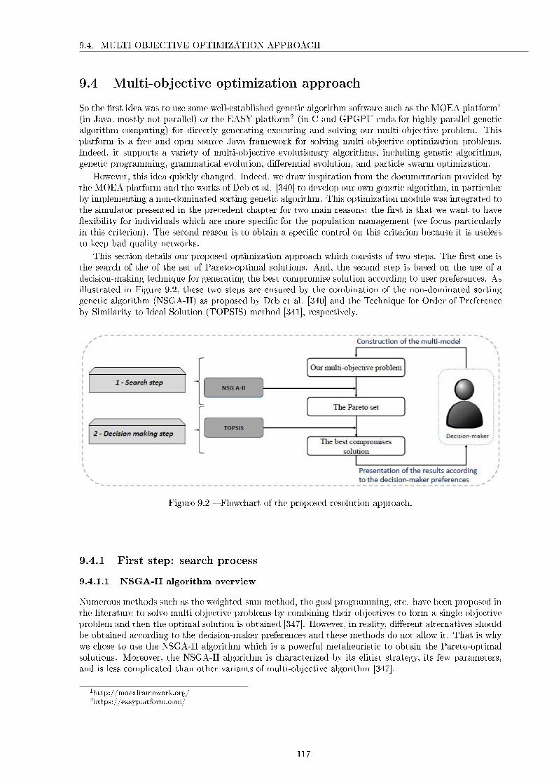
9.4. MULTI-OBJECTIVE OPTIMIZATION APPROACH
9.4 Multi-objective optimization approach
So the �rst idea was to use some well-established genetic algorithm software such as the MOEA platform1
(in Java, mostly not parallel) or the EASY platform2 (in C and GPGPU cuda for highly parallel geneticalgorithm computing) for directly generating executing and solving our multi-objective problem. Thisplatform is a free and open source Java framework for solving multi-objective optimization problems.Indeed, it supports a variety of multi-objective evolutionary algorithms, including genetic algorithms,genetic programming, grammatical evolution, di�erential evolution, and particle swarm optimization.
However, this idea quickly changed. Indeed, we draw inspiration from the documentation provided bythe MOEA platform and the works of Deb et al. [340] to develop our own genetic algorithm, in particularby implementing a non-dominated sorting genetic algorithm. This optimization module was integrated tothe simulator presented in the precedent chapter for two main reasons: the �rst is that we want to have�exibility for individuals which are more speci�c for the population management (we focus particularlyin this criterion). The second reason is to obtain a speci�c control on this criterion because it is uselessto keep bad quality networks.
This section details our proposed optimization approach which consists of two steps. The �rst one isthe search of the of the set of Pareto-optimal solutions. And, the second step is based on the use of adecision-making technique for generating the best compromise solution according to user preferences. Asillustrated in Figure 9.2, these two steps are ensured by the combination of the non-dominated sortinggenetic algorithm (NSGA-II) as proposed by Deb et al. [340] and the Technique for Order of Preferenceby Similarity to Ideal Solution (TOPSIS) method [341], respectively.
Figure 9.2 � Flowchart of the proposed resolution approach.
9.4.1 First step: search process
9.4.1.1 NSGA-II algorithm overview
Numerous methods such as the weighted-sum method, the goal programming, etc. have been proposed inthe literature to solve multi-objective problems by combining their objectives to form a single objectiveproblem and then the optimal solution is obtained [347]. However, in reality, di�erent alternatives shouldbe obtained according to the decision-maker preferences and these methods do not allow it. That is whywe chose to use the NSGA-II algorithm which is a powerful metaheuristic to obtain the Pareto-optimalsolutions. Moreover, the NSGA-II algorithm is characterized by its elitist strategy, its few parameters,and is less complicated than other variants of multi-objective algorithm [347].
1http://moeaframework.org/2https://easyplatform.com/
117

9.4. MULTI-OBJECTIVE OPTIMIZATION APPROACH
9.4.1.2 NSGA-II algorithm operation
Similarly to a simple genetic algorithm, the NSGA-II algorithm starts by generating a random set ofsolutions called population. This population consists of a set of individuals also called chromosome. Thepopulation has a size Np which is an important parameter in the NSGA-II. Then, the objective functionsare evaluated for each individual and ranked based on the concept of non-domination (if a solution cannotimprove any objective value without degrading one or more of the other objective values). After that,the o�spring population is created using the selection, crossover and mutation operators. Then, thebest chromosomes are selected using the elitism operator. These steps are repeated until the stoppedcondition is reached. Finally, the output of the algorithm is a set of solutions that should be near thePareto-optimal.
9.4.1.3 Genetic algorithm implementation
Here, we explain and detail the steps of the genetic algorithm implementation. The logical diagram ofthe employed multi-objective genetic algorithm on the basis of NSGA-II is given in Figure 9.3 and itsoperation is detailed in Algorithm 6. As well as, the genetic algorithm operators were carefully selectedbased on the requirements of the transittability problem.
Figure 9.3 � Flowchart of the proposed multi-objective optimization method based on the NSGA-IIalgorithm.
118

9.4. MULTI-OBJECTIVE OPTIMIZATION APPROACH
Chromosome encoding In our context, the representation of a chromosome consists of a list of stimuli.An individual is a couple with the �rst part the stimuli and in the second part the time of its introduction.These stimuli are part of the biological data imputed by biologists and which are de�ned by di�erentproperties such as the index of the stimuli Si, the time of introduction of the stimulus Si into the nodemi, the target node mi by the stimulus Si, the variation of concentration caused by the stimulus Si onthe node mi, the cost of the stimulus Si, and the discomfort caused by the stimulus DiscomfortStimk.Figure 9.4 illustrates the chromosome encoding considered for an example with S = 15. This example ofstimuli and their properties can be found in Table 10.2.
Figure 9.4 � Chromosome encoding.
Initial population Initially, the chromosomes are generated randomly creating a �rst population P0
(gen = 0) with a population of size Np. The objective functions from Equations (1) to (4) are evaluatedfor each chromosome respectively. Then, the parent population are ranked based on the non-dominationconcept. In a second step, a child population Q0 (gen = gen + 1) of size Np is created from the parentpopulation P0 by the use of the selection, crossover and mutation operators.
Selection (NSGA-II) Considering the obtained chromosomes, the population is sorted based on thenon-domination principle. This elitism method consists: (i) �rstly in searching the dominated individualsin the population and ranking them according to their dominance using Equation (17) (where X and Yare two individuals and xi, yi are objective functions). Then, (ii) the selection of those which have thegreater rank. In the case of two individuals with the same rank of dominance, we compute the crowdingdistance between them as de�ned by Equation (18) (where d(k) is the crowding distance of individualk, fkj is the jth objective function value of the kth individual, and fminj , fmaxj are the minimum andmaximum value of the jth objective function, respectively). Indeed, the crowding distance value of asolution provides an estimation of the density of solutions surrounding that solution. In other words, thecrowding distance value of a particular solution is the average distance of its two neighbouring solutions.It is a measure of "density of solutions surrounding a particular solution in the population" [340]. Theindividual having the greater crowding distance value is better than those having a small value.
∀X = {x1, . . . , xM} and Y = {y1, . . . , yM} Then X � Y ⇔ ∀i : xi ≤ yi and ∃j : xj ≤ yj (17)
d(k) =∑Mj=1
|fk+1j −fk−1
j |fmaxj −fmin
j(18)
Crossover To perform the crossover, two parents are randomly selected. A point, representing herethe time of introduction of a stimulus, is randomly selected and designated as the crossover point. Then,the stimuli that are very next to the crossover point are interchanged. Finally, o�spring chromosomes
119
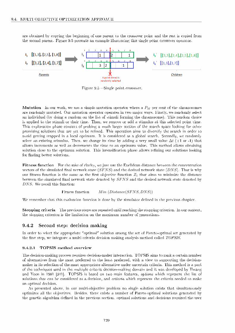
9.4. MULTI-OBJECTIVE OPTIMIZATION APPROACH
are obtained by copying the beginning of one parent to the crossover point and the rest is copied fromthe second parent. Figure 9.5 presents an example illustrating this single point crossover operator.
Figure 9.5 � Single point crossover.
Mutation In our work, we use a simple mutation operator where a PM per cent of the chromosomesare randomly mutated. Our mutation operator operates in two major ways. Firstly, we randomly selectan individual (by doing a random on the list of stimuli forming the chromosome). This random choiceis applied to the stimuli or their time. Then, we remove or add a stimulus at this selected point time.This exploration phase consists of probing a much larger section of the search space looking for otherpromising solutions that are yet to be re�ned. This operation aims to diversify the search in order toavoid getting trapped in a local optimum. It is considered as a global search. Secondly, we randomlyselect an existing stimulus. Then, we change its time by adding a very small value ∆t (+1 or -1) thatallows increments as well as decrements the time to an optimum value. This method allows obtainingsolution close to the optimum solution. This intensi�cation phase allows re�ning our solutions lookingfor �nding better solutions.
Fitness function For the sake of clarity, we just use the Euclidean distance between the concentrationvectors of the simulated �nal network state (SFNS) and the desired network state (DNS). That is whyour �tness function is the same as the �rst objective function Z1 that aims to minimize the distancebetween the simulated �nal network state denoted by SFNS and the desired network state denoted byDNS. We recall this function:
Fitness function = Min (Distance(SFNS,DNS))
We remember that this evaluation function is done by the simulator de�ned in the previous chapter.
Stopping criteria The previous steps are repeated until reaching the stopping criterion. In our context,the stopping criterion is the limitation on the maximum number of generations.
9.4.2 Second step: decision making
In order to select the appropriate "optimal" solution among the set of Pareto-optimal set generated bythe �rst step, we integrate a multi-criteria decision-making analysis method called TOPSIS.
9.4.2.1 TOPSIS method overview
The decision-making process requires decision-maker interaction. TOPSIS aims to rank a certain numberof alternatives from the most preferred to the least preferred, with a view to supporting the decision-maker in its selection of the most appropriate alternative under uncertain criteria. This method is a partof the techniques used in the multiple criteria decision-making domain and it was developed by Hwangand Yoon in 1981 [341]. TOPSIS is based on two main features, options which represent the list ofsolutions that can be considered as a decision, and criteria which represent the criteria needed to makean optimal decision.
As presented above, in our multi-objective problem no single solution exists that simultaneouslyoptimizes all the objectives. Besides, there exists a number of Pareto-optimal solutions generated bythe genetic algorithm de�ned in the previous section. optimal solutions and decisions required the user
120

9.4. MULTI-OBJECTIVE OPTIMIZATION APPROACH
Algorithm 6 Pseudocode of the employed non-dominated sorting genetic algorithm (NSGA-II) [340]
Require: The parent population P = ϕ; The child population Q = ϕ; The collect population R = ϕ;The generation index population gen = 0; The maximum number of generation MaxGen
Ensure: The populations P are the non-dominated solutions1: Randomly initialize the parent population P0.2: while stopping condition not satis�ed (gen < Maxgen) do3: Combine the parent and child populations Rgen = Pgen ∪Qgen4: Rank individuals of Rgen to obtain the non-dominated fronts: F = fast-non-dominated (Rgen)5: Pgen + 1 = ϕ and i = 16: while the parent population size |Pgen + 1|+ |Fi| < N do7: Compute the crowding-distance of Fi8: Add the ith non-dominated front Fi to the parent population Pgen + 19: i = i+ 110: end while11: Rank the Fi according to the crowding distance12: Complete the parent population Pgen + 1 with the �rst N − |Pgen + 1| elements of Fi13: Generate the child population Qgen + 114: gen = gen+ 115: end while
intervention and need to be taken in the presence of trade-o�s among all our objective functions. Suchdecision-making involves confronting trade-o�s between multiple, con�icting objectives or criteria. In thetransittability problem, the user is confronted with �ve objective functions, even contradictory, and withsubjective and objective criteria in any mix. This requires to consider the user preferences. What makesthe decision task more di�cult. For these reasons, we integrate the TOPSIS method to our optimizationmodule. Indeed, this method o�ers more �exibility and freedom to the decision-maker considering itspreferences. The user selects amongst the objective functions which of them are to be used as objectivefunctions, albeit he can use them all, but also has the possibility to associate weights according totheir relative importance. Moreover, this method takes into account additional subjective preferenceinformation, this allows classifying the Pareto-optimal solutions obtained in the search step by sortingthem in order of priority according to the decision-maker preferences.
9.4.2.2 TOPSIS method operation
According to the preferences given by the decision-maker, the TOPSIS method will select the appropri-ate "optimal" solution (among the set of Pareto-optimal solution) that is close to its preferences andrequirements. In our context, the Pareto-optimal set constitutes the alternatives of the TOPSIS method.Its principle consists on compute �rstly the distance measure among the di�erent alternatives to de�nethe ideal and negative-ideal solution. The distance between the ideal point and each alternative canbe calculated using Eq. (19). Using the same separation measure, the distance between the negativeideal point and each alternative can be determined (Eq. (20)) [348]. The relative closeness to the idealpoint can be calculated using Eq. (21). Where vij is the weighted standardized criterion value of the ith
alternative that is calculated by multiplying standardized criterion value by the corresponding weight,and v+j is the ideal value and v−j is the negative ideal value for the jth criterion [348].
Si+ = [∑nj=1(vij − v+j)2] (19)
Si− = [∑nj=1(vij − v−j)2] (20)
ci+ = Si−Si++Si−
(21)
Then, it associates to each alternative a numerical coe�cient between 0 and 1 according to theEuclidean distances between each alternative on the one hand, and the ideal and negative-ideal solutionson the other hand. Next, it ranks the alternatives (their measures) according to the importance of theattribute starting by the appropriate alternative (that have the shortest distance from the ideal solutionand the longest distance from the negative-ideal solution) to the bad one [349]. This is how the Pareto-optimal solutions are ranked, compared and proposed to the decision-maker order by its preferences.
121

9.5. SUMMARY
Algorithm 7 Pseudocode of the TOPSIS technique
1: Establish a matrix of criteria and di�erent alternatives2: Normalize the decision matrix3: Compute the weight of the normalized decision matrix4: Determine the ideal solutions and nadir solution (negative ideal solution)5: Compute the distance for each alternative6: Compute the relative closeness to the ideal solution7: Rank the preference order
Algorithm 7 depicted the pseudo-code of the TOPSIS decision-making technique. In our problem, thealternatives of the TOPSIS are the set of Pareto-optimal solution generated by the search step (they arethe options which are to be evaluated for selection the best). The criteria are our �ve objective functions,the minimization of the distance between the simulated �nal network state and the desired network state,the minimization of the number of input signals, the minimization of the cost of these external stimuli,the minimization of the number of target nodes and the minimization of the patient discomfort (thesewill impact the selection of alternatives). In this method, two properties should be considered:
• The completeness: it is important to ensure that all the criteria are included.
• The operationality: it is important that each alternative can be judged against each criterion.
To each criterion, we associate a weight that will estimate the relative importance of this objectivefunction. All the TOPSIS steps (summarized in Algorithm 7) are detailed in the Wikipedia encyclopedia3.
9.5 Summary
The transittability of complex biomolecular networks is a multi-criteria problem by nature since thereare several potentially con�icting criteria to consider while steering the network from an initial state toa desired state. In this chapter, �ve essential criteria, which need to be minimized simultaneously tosteer complex biomolecular networks, are presented and described in detail. There is the minimization ofthe distance between the simulated �nal network state and the desired network state, the minimizationof the number of input signals, the minimization of the cost of these external stimuli, the minimizationof the number of target nodes and the minimization of the patient discomfort. Applying a minimumnumber of external stimuli on a minimum number of steering nodes has been already considered inexisting mathematical models in the literature, however, these criteria are not su�cient for completelysteering complex biomolecular networks. That is why other criteria have been considered in this proposedmathematical model.
Moreover, in this chapter, a multi-objective optimization approach for solving this problem has beenproposed and detailed. This optimization approach consists of two steps: the search and decision-makingsteps. The search step is based on a powerful multi-objective genetic algorithm, the NSGA-II, to solveour problem and obtain a Pareto-optimal set. Indeed, we draw inspiration from the documentationprovided by the MOEA platform and the works of Deb et al. [340] to develop our own genetic algorithm,in particular by implementing a non-dominated sorting genetic algorithm. While the decision-makingstep is based on a multi-criteria decision-making method, the TOPSIS, to compare the Pareto-optimalsolutions and provide the decision-maker with the best compromise solution according to its preferences.
This optimization module was integrated to the simulator presented in the precedent chapter for twomain reasons: the �rst is that we want to have �exibility for individuals which are more speci�c for thepopulation management (we focus particularly in this criterion). The second reason is to obtain a speci�ccontrol on this criterion because it is useless to keep bad quality networks.
The next part is devoted to the validation of our proposed approaches.
3https://en.wikipedia.org/wiki/TOPSIS
122

Part III
Experiments and discussion
From Chapter 6 to Chapter 9, we have introduced the four contributions for achieving the overall goal of thisstudy, which is to propose a platform that enables biologists to simulate the state changes of biomolecular
networks with the goal of steering their behaviours.In order to verify the proposed approaches, a prototype intituled CBNSimulator, which combines the function ofthe approaches stated above in Part II, has been developed. In Chapter 10, we illustrate the potential of the
prototype based on three case studies. This chapter also introduces the prototype interfaces and features. Then,in Chapter 11, we evaluate and discuss the performance of our proposed approaches according to the results
obtained by exploiting the case studies.This part is divided into two chapters:
10 Prototype: the CBNSimulator ................................................................................12511 Evaluation .......................................................................................................................149
123


Chapter 10
Prototype: the CBNSimulator
Contents10.1 Introduction . . . . . . . . . . . . . . . . . . . . . . . . . . . . . . . . . . . . . 126
10.2 Aims of the CBNSimulator platform . . . . . . . . . . . . . . . . . . . . . . . 126
10.3 Overview of the CBNSimulator platform . . . . . . . . . . . . . . . . . . . . 126
10.4 Development tools . . . . . . . . . . . . . . . . . . . . . . . . . . . . . . . . . . 128
10.5 Experimental results . . . . . . . . . . . . . . . . . . . . . . . . . . . . . . . . 128
10.5.1 Case study 1: the bacteriophage T4 gene 32 . . . . . . . . . . . . . . . . . . . . 128
10.5.2 Case study 2: the control of the lifecycle of bacteriophage lambda . . . . . . . 129
10.5.3 Case study 3: the p53-mediated DNA damage response network . . . . . . . . 137
10.6 Summary . . . . . . . . . . . . . . . . . . . . . . . . . . . . . . . . . . . . . . . 145
125

10.1. INTRODUCTION
10.1 Introduction
From Chapter 6 to Chapter 9, we have detailed the di�erent contributions for modelling, simulating,understanding and optimizing the transittability of complex biomolecular networks. Indeed, Chapter 6introduces the proposed logic-based modelling for describing the di�erent elements required for modellingthe transittability of biomolecular networks following the systems theory. Chapter 7 enhances this logic-based modelling with an additional semantic layer to obtain an optimal and more realistic modellingdescribing the structure, function, behaviour and semantic of complex biomolecular networks. Both ofthese Chapters 6 and 7 are the foundations of the simulator presented in Chapter 8 that deals with aqualitative, discrete-time simulation for reproducing the behaviour of complex biomolecular networks.Finally, Chapter 9 presents a multi-objective optimization approach for solving the transittability ofcomplex biomolecular networks.
In order to verify these contributions, we provide biologists with a �exible platform called the 'CB-NSimulator' which combines the function of the four approaches stated above. This chapter focus onpresenting the CBNSimulator as an innovative multi-domain collaborative platform for the modelling,simulating, understanding and optimizing of complex biomolecular networks. The �rst section presentsits main objectives. The general architecture of the proposed platform is explained in the second section.The environment and tools for its implementation are illustrated in the third section. The last sectionillustrates the advantages of this platform by applying it to three widely studied biomolecular networks,the autoregulation of the bacteriophage T4 gene 32 network, the control of the phage lambda infectionof bacteria and the p53-mediated DNA damage response network.
10.2 Aims of the CBNSimulator platform
The main goals of the CBNSimulator platform can be grouped into four important points:
1. The logical modelling of complex biomolecular networks.The main goal of the proposed CBNSimulator is to produce a whole-cell computational model.This computational model consists of a logic-based modelling that aims to represent, analyze andinterpret the complex structure, the di�erent functional aspects, and the dynamic behaviour ofthese multi-level biomolecular networks.
2. The semantic modelling of complex biomolecular networks.The second purpose of the CBNSimulator aims to provide a rich semantic description of the transit-tability of biomolecular networks. This semantic modelling should infer more knowledge about thefunctioning of biomolecular networks and provides the new knowledge required in understandingtheir behaviours and their state changes.
3. The simulation of the behaviour of complex biomolecular networks.The third goal of the CBNSimulator platform is to reproduce the conditions of the evaluatedbiomolecular network and its components over time. This simulation should predict the importantproperties of biomolecular networks even when quantitative data of such networks are unavailableor unknown.
4. The optimization of the transittability of complex biomolecular networks.The last goal of the CBNSimulator is to provide biologists with a tool that is able to control andguide the behaviour and the transition states of complex biomolecular networks. In other words, byoptimizing the steering of complex biomolecular networks form their actual state to a desired statetaking into account di�erent constraints such as, the distance between the simulated �nal networkstate and the desired network state, the number of external stimuli, their cost, the number of targetnodes and the patient discomfort.
10.3 Overview of the CBNSimulator platform
CBNSimulator provides a series of facilities (i) to model and simulate a given biomolecular networkformalised through a logic-based model and semantically described through a semantic modelling, and
126

10.3. OVERVIEW OF THE CBNSIMULATOR PLATFORM
(ii) to steer these networks from their actual state to a desired state under speci�c and controlledconditions. As illustrated in Figure 10.1, the platform is organized into four main modules: the logicmodelling module, the ontological module, the simulation module, and the optimization module.
Figure 10.1 � Overall architecture of the CBNSimulator platform.
1. The logic modelling module: It represents the starting point for any new user-de�ned biomolecularnetwork. It has been designed to provide all the necessary elements for modelling the biomolecularnetwork by considering its di�erent levels and molecular components. For example, the user canspecify the list of molecular components and their corresponding type, the list of interactions amongthese components and their corresponding conditions that activate them, etc. This logic-basedmodelling takes into account the complexity and heterogeneity of these molecular components andtheir multilevel structure.
2. The ontological module: It ensures the management, modelling and sharing of expert knowledge.This module takes as input all the native information introduced by the expert (state of the network,its structure, etc.) through the logic-based formalization provided by the �rst module. Then,the ontological module provides output inferred network that is composed of native and inferredknowledge. This represents useful features, especially when the logic-based model lacks these details.Moreover, the additional information provided by this module about the network's elements can beused to identify new potential relationships among them.
3. The simulation module: It allows users to simulate and/or reproduce the dynamical behaviour ofthe network. Indeed, this simulator integrates all the information given by the expert (the enrichednetwork with native and inferred knowledge) with other parameters in order to better reproducethe conditions of the evaluated biomolecular network and its components over time. The resultsgenerated during the simulation may be displayed to the users in graphical form to facilitate theirinterpretation, or used by the optimization module.
4. The optimization module: It provides a way to steer the states of the network from its actualstate to another speci�c state. This optimization is performed by specifying the initial and desiredstates of the network, and all the possible external stimuli de�ned by the user. Then, based onthe values of the evaluation criteria, this module provides the best transition sequences for steeringthe biomolecular network from its initial state to the desired state and, �nally, presents the resultsaccording to the user preferences. This model allows also to optimize the transittability of thenetwork by minimizing various criteria, such as the distance between the simulated �nal network
127

10.4. DEVELOPMENT TOOLS
state and the desired network state, the number of external stimuli, their cost, the number of targetnodes and the patient discomfort.
10.4 Development tools
In this section, we present the di�erent software used for developing the CBNSimulator platform:
• Java Platform, Standard Edition (Java SE)1 The platform uses Java programming language andis part of the Java software-platform family. Java is particularly well-suited for creating complexanalytical applications and architecture.
• Eclipse2 It is an integrated development environment for developing with Java, but it may also beused to develop applications in other programming languages via plug-ins. It is the most widelyused Java IDE. Eclipse contains a base workspace and an extensible plug-in system for customizingthe environment. Considering the features of the CBNSimulator platform, that is, a frame-basedJava SE application, Eclipse Luna Service Release 2 (4.4.2) is chosen as the environment for itsimplementation.
• Protégé3 It is a free, open source ontology editor and knowledge-base framework building intelligentsystems. As well as the Protégé editor supports modelling ontologies through a web client ordesktop client. Protégé supports various ontologies formats, such as, RDF, RDF Schema, XMLSchema and OWL. In our researches, the proposed ontologies have been implemented within theProtégé 5 environment, version 1.3.8.3.
10.5 Experimental results
In order to better explain how CBNSimulator can be applied for modelling, simulation and optimizationof complex biomolecular networks, we analysed, as case studies, the autoregulation of the bacteriophageT4 gene 32 [318], the control of lifecycle of bacteriophage lambda [350], and the p53-mediated DNAdamage response network (cell fate decision) [6].
10.5.1 Case study 1: the bacteriophage T4 gene 32
This case study has already been used as a motivating example along the contributions clarifying theirnotions. Indeed, it should be mention that along with our contributions, this example has been presentedas a three-node network consisting of the gene 'G32', the protein 'p32' and the metabolite 'm32'. Thenode m32 has been arbitrarily added in order to highlight the di�erent level of cell's components (gene,protein and metabolite) and to better explain our contributions. Here, to conform to biology, we treatthe original network which is only the gene 'G32' and the protein 'p32'. We chose this case study due toits simplicity and its well-known mechanism.
10.5.1.1 Description
The bacteriophage T4 gene 324 encodes a single-stranded DNA binding protein required for T4 DNAreplication, recombination, and repair [318]. It is a single polypeptide chain of 301 amino acid residuesthat consists of three structural domains, each of which has a binding function. Despite its role in DNAmetabolism, the gene product 32 autoregulates its synthesis at the level of translation [319]. During theinfection, the gene product 32 is produced in large amounts to perform its function of binding all availableDNA at the replication fork, recombination nodes and at lesions in DNA resulting from damage [320].When all the available DNA is bound, free gene product 32 accumulates within the cell until it reachesa certain concentration which then attenuates further synthesis of gene product 32 [321]. More detailabout the bacteriophage T4 gene 32 can be found in [318, 320, 321].
1https://www.oracle.com/fr/java/technologies/java-se.html2https://www.eclipse.org/3http://www.hermit-reasoner.com/4http://genes.atspace.org/10.11.html
128

10.5. EXPERIMENTAL RESULTS
As illustrated in Figure 10.2, this biomolecular network consists of two nodes a gene G32 coding fora protein p32, which in turn can inhibits or activates the gene G32 according to the value of its ownconcentration. Therefore, in this network, the concentration of p32 is self-regulated and normally shouldremain between 0.2 10−6 mol/dm3 and 0.7 10−6 mol/dm3. When the concentration of p32 exceedsthe threshold Sp32 = 0.7 10−6 mol/dm3, it is called an Inhibition, i.e. the protein p32 inhibits, ordeactivates, the translation of its gene G32. However, when the concentration of p32 decreases andbecomes lower than the threshold Sp32 = 0.2 10−6 mol/dm3, it is called an Activation, i.e. the proteinp32 activates the translation of its gene G32. When the gene G32 is activated by the protein p32, it iscalled a Translation, in which we have a production of p32 thus increasing the value of its concentration.
Figure 10.2 � The bacteriophage T4 gene 32 use case.
10.5.1.2 Logical modelling
The logic modelling of the bacteriophage T4 gene 32 is illustrated in Table 6.4 (Section 6.5).
10.5.1.3 Semantic modelling
The sematic modelling of the bacteriophage T4 gene 32 was already detailed in Section 7.4. Indeed, wepresent the instantiation of the BNO ontology for the given example in Figure 7.5. We highlight also thedi�erent properties of the instantiation its components (the gene G32, protein p32 and metabolite m32)in Figure 7.6. We describe also the instantiations of its four interactions in Figure 7.7.
Moreover, we use the BNO ontology to simulate the behaviour of its components. To do this, we usean SWRL rule-based reasoner, and we develop some SWRL rules such as the inhibition SWRL rule andits opposite rule, activation SWRL rule and its opposite, the transcription SWRL rule and its oppositerule, and the negative regulation SWRL rule and its opposite rule. Results of these rules are illustratedin Figures 7.8, 7.9, 7.10, 7.11, 7.12, 7.13, respectively.
10.5.1.4 Simulation under the CBNSimulator
The simulation results of the bacteriophage T4 gene 32, provided by the CBNSimulator, were syntheticallyrepresented in graphical form in Figure 8.5. These results were formally treated and validated by expertbiologists. Indeed, these results correspond to their domain knowledge and the real behaviour of thenetwork.
10.5.2 Case study 2: the control of the lifecycle of bacteriophage lambda
The control of the lifecycle of bacteriophage lambda infection is one of the best understood regulatorysystems [350]. We use this the phage lambda because it is a simple and realistic case study with a well-known mechanism. Indeed, its functioning was investigated by several studies such as [350, 351, 352, 353,354, 355].
129

10.5. EXPERIMENTAL RESULTS
10.5.2.1 Description
The phage lambda5 is a virus that infects the bacteria Escherichia Coli. It is called a temperate bacterio-phage, because it can alternate between two possible developmental pathways: the lytic cycle and thelysogenic cycle under certain conditions [355]. During the lytic cycle, the phage infects the bacteria:its DNA is replicated in large quantities within the bacteria to make lots of phages, and then kills thecell by making it explode (its destruction). During the dormant lysogenic cycle, the phage inserts itsDNA into the bacterial chromosome allowing the phage DNA (called also prophage) to be copied and thecell continues to reproduce normally [350]. Figure 10.3 illustrates the switching between the lytic andlysogenic phase. Indeed, during the infection, the phage lambda have two choices: (i) replicate and killthe host cell (Lysis) or (ii) integrate into the bacterial chromosome, where it replicates as a part of thecell genome (Lysogeny) [5]. The phage lambda state generally in the lysogenic phase. However, when itis in the lysogen phase it can be switched to the lytic phase through ultraviolet stimuli.
Figure 10.3 � The lifecycle of bacteriophage lambda. (inspired from [5])
As illustrated in Figure 10.4, this biomolecular network consists of six nodes: four genes G_CI,G_OR3, G_OR1, G_CRO, and two proteins P_CI, and P_CRO. During the lytic phase, thegene G_CI is activated (and G_CRO is deactivated). This activation of the gene G_CI generates itstranscription by producing a protein P_CI. When the concentration of this protein reached a thresholdequal to 0.1, it deactivates the gene G_OR1, which in turn deactivates the gene G_CRO (this providesthe lysogenic phase). Then, when the gene G_CRO gene is deactivated, there is no production of theprotein P_CRO. The expression of lysogenic genes (G_CRO and G_OR1) is therefore deactivated. Inthis case, we are totally in the lytic phase. After a certain time in this lytic state, the destruction of thehost cell occurs. For reason of clarity, we reduce this functioning in a set of rules (the black arrows inFigure 10.4) as follows:
1. When the gene G_CI is activated, there is a transcription of the protein P_CI.
2. Once the protein concentration reached P_CI] > 0.1, it inhibits the gene G_OR1.
3. When the gene G_OR1 is deactivated, it deactivates the gene G_CRO.
4. Once the gene G_CRO is deactivated, there is an absence of transcription.
On the other hand, in the lysogenic phase the gene G_CRO is activated (and G_CI is deactivated).This activation of the gene G_CRO generates its transcription by producing a protein P_CRO. When
5https://cshmonographs.org/index.php/monographs/issue/view/087969102.2
130

10.5. EXPERIMENTAL RESULTS
the concentration of this protein reached a threshold equal to 0.2, it deactivates the gene G_OR3, whichin turn deactivates the gene G_CI (this provides the lytic phase). Then, when the gene G_CI isdeactivated, there is no production of the protein P_CI. The expression of lytic genes (G_CI andG_OR3) is therefore deactivated. In this case, we are totally in the lysogenic phase. The state of thephage lambda stays at this state even in the absence of ultraviolet stimuli. For reason of clarity, wereduce this functioning in a set of rules (blue arrows in Figure 10.4) as follows:
1. When the gene G_CRO is activated, there is a transcription of the protein P_CRO.
2. Once the protein concentration reached P_CRO > 0.2, it inhibits the gene G_OR3.
3. When the gene G_OR3 is deactivated, it deactivates the gene G_CI.
4. Once the gene G_CI is deactivated, there is anabsence of transcription.
Figure 10.4 � Functioning rules of the phage lambda.
10.5.2.2 Logic-based modelling
Table 10.1 presents the structure and the function of the logical modelling of the phage lambda. Itscausal graph is given by Figure 10.4. The possible states that can have the phage lambda network duringthe simulation are represented by the behaviour CR, as illustrated by Figure 10.5:
Figure 10.5 � An excerpt of the possible states that can have the phage lambda network during thesimulation.
10.5.2.3 Semantic modelling
Here, we use OWL and SWRL rules for semantically modelling our case study and simulating its be-haviour. To do this we instantiate our ontology for the given example. Figure 10.6 depicted the BNOindividuals' of the phage lambda considering their various characteristics. The molecular components
131

10.5. EXPERIMENTAL RESULTS
and the interactions that occur among them are represented by individuals and corresponding relations.The relations are restricted by specifying domain and range. All the concepts and individuals are linkedto primitive data (concentrations values, genes states, etc.) through the data properties. This semanticmodelling provides all the elements for modelling the states and the individuals behaviours of phagelambda through the use of SWRL rules. This set of SWRL rules is able to reason and simulate thebehaviour of the phage lambda. The following paragraphs demonstrate the simulation of the given casestudy using SWRL rules.
Figure 10.6 � Semantic modelling of the phage lambda within the Protégé editor. The molecular compo-nents: A- G_CI, B- G_CRO, C- G_OR3, D- G_OR1, E- P_CI, F- P_CRO. Some interactions: a-i3, b- i7, c- i2, d- i6, e- i1, f- i5.
Inhibition SWRL rule between proteins and genes (interactions i2 and i6) The followingrule models the inhibition interaction that occurs between the proteins P_CI, P_CRO and the genesG_OR1, G_OR3, respectively. When the concentration of the proteins (P_CI and P_CRO) exceedsthe threshold 0.2 10−6 Mol/L−1, they inhibit the translation of their targeted genes (G_OR1 andG_OR3).
132

10.5. EXPERIMENTAL RESULTS
ADN(?g) ∧ hasState(?g, ?gs1) ∧ forTime(?gs1, ?t) ∧ hasState(?g, ?gs2) ∧ forTime(?gs2,?t2) ∧ swrlb:add(?t2, ?t, 1) ∧ Protein(?p) ∧ Inhibition(?inhi) ∧ hasSource(?inhi, ?p) ∧hasEnd(?inhi, ?g) ∧ hasState(?p, ?ps) ∧ forTime(?ps, ?t) ∧ hasConcentrationValue(?ps,?c) ∧ swrlb:greaterThanOrEqual(?c, 0.7) → isActivated(?gs2, false)
The results of this rule means that, If there is a protein p having a state ps equal to a concentrationc at a given time t and there is a gene g having a state gs equal to true at this time t, and these twomolecules p and g are related by an Inhibition interaction, and if the concentration c of the protein pexceeds a threshold equal to 0.2, then the state of g move to false at time t+ 1. We treat for example the
Figure 10.7 � Results of the reasoning process for the Inhibition SWRL rule between the proteins andtheir targeted genes.
case of the inhibition that occurs between the protein P_CRO and the gene G_OR3. As illustrated inFigure 10.7, we �rstly, activate the gene G_OR3 and set the value of the concentration of the proteinP_CRO at 0.4 10−6 Mol/L−1 at time t = 22. Then, when we launch the reasoner, we note that attime t = 23 the gene G_OR3 is automatically deactivated (because the value of the concentration of theprotein P_CRO exceeds the threshold 0.2).
Inhibition SWRL rule between genes (interactions i3 and i7) The following rule models theinhibition interaction between the genes G_OR1 and G_CRO, and between G_OR3 and G_CI. Whenthe concentration of the a gene (the staring node) is deactivated, it inhibits its targeted gene (deactivatesthe targeted node). This s the case of the two interactions i3 and i7.
ADN(?g) ∧ hasState(?g, ?gs) ∧ forTime(?gs, ?t) ∧ isActivated(?gs, false) ∧ swrlb:add(?t2,?t, "1"8sd:int) ∧ ADN(?g2) ∧ InhibitionGG(?in) ∧ hasSource(?in, ?g) ∧ hasEnd(?in,?g2) ∧ hasState(?g2, ?g1s) ∧ forTime(?g1s, ?t) ∧ isActivated(?g1s, true) ∧ hasState(?g2,?g2s) ∧ forTime(?g2s, ?t2) → isActivated(?g2s, false)
The results of this rule means that, If there is a gene g having a state gs equal to true at a given time tand there is another gene g1 equal to false at this time t, and these two molecules g and g1 are related byan Inhibition interaction, then the state of the targeted gene g move to false at time t+ 1. For example,we treat the case of the interaction i7 that occurs between the genes G_OR3 and G_CI. As depicted inFigure 10.8, we �rstly, activate the gene G_CI and deactivate the gene G_OR3 at time t = 25. Then,when we launch the reasoner, we note that at time t = 26 the gene G_CI is automatically deactivated.
133

10.5. EXPERIMENTAL RESULTS
Figure 10.8 � Results of the reasoning process for the Inhibition SWRL rule between genes.
Transcription SWRL rule (interactions i1 and i5) The following rule represents the gene tran-scription. In our case study, we have two transcription interactions i1 and i5. In fact, if the genes G_CIand G_CRO are activated, these ones generates the proteins synthesis and produce an increase in theconcentration of these proteins P_CI and P_CRO.
ADN(?g) ∧ hasState(?g, ?gs) ∧ forTime(?gs, ?t) ∧ isActivated(?gs, true) ∧ Protein(?p)∧ Transcription(?trans) ∧ hasSource(?trans, ?g) ∧ hasEnd(?trans, ?p) ∧ hasState(?p,?ps1) ∧ forTime(?ps1, ?t) ∧ hasConcentrationValue(?ps1, ?c1) ∧ hasState(?p, ?ps2) ∧forTime(?ps2, ?t2) ∧ swrlb:add(?t2, ?t, 1) → hasConcentrationValue(?ps2, ?c2)
The result of this rule is interpreted as follows, If there is a gene g having a state gs equal to true at agiven time t and there is a protein p having a state ps1 and a concentration c at this time t, and thesetwo molecules g and p are related by a Transcription interaction, then the concentration of the proteinp increases at time t + 1. In Figure 10.9, we treat the transcription of the interaction i1 that occursbetween the gene G_CI and the protein P_CI. Firstly, we set the value of the concentration of theprotein P_CI at 0.6 10−6 Mol/L−1 and activate the gene G_CI at time t = 30. Then, when we launchthe reasoner, we note that the value of the concentration of the protein P_CI increases automaticallyto 0.7 10−6 Mol/L−1 at time t = 31.
In the opposite case, the case corresponding to the interactions i4 and i8 showing an inhibitioninteraction between the genes G_CI and G_CRO the proteins P_CI and P_CRO, respectively. Wehave this rule in which there is not transcription and the concentration of the protein is maintained stable:
ADN(?g) ∧ hasState(?g, ?gs) ∧ forTime(?gs, ?t) ∧ isActivated(?gs, false) ∧ Protein(?p)∧ Transcription(?trans) ∧ hasSource(?trans, ?g) ∧ hasEnd(?trans, ?p) ∧ hasState(?p,?ps1) ∧ forTime(?ps1, ?t) ∧ hasConcentrationValue(?ps1, ?c1) ∧ hasState(?p, ?ps2) ∧forTime(?ps2, ?t2) ∧ swrlb:add(?t2, ?t, 1) → hasConcentrationValue(?ps2, ?c1)
The result of this rule means that, If there is a gene g having a state gs equal to false at a given time tand there is a protein p having a state ps1 and a concentration c at this time t, and these two moleculesg and p are related by a Transcription interaction, then the concentration of the protein p remains stableat time t+ 1.
10.5.2.4 Simulation under the CBNSimulator
The CBNSimulator also provides a powerful simulator based on both (i) the qualitative, discrete-eventsimulation theory and (ii) the merging of the logic-based and semantic modelling. This simulation module
134

10.5. EXPERIMENTAL RESULTS
Figure 10.9 � Results of the reasoning process for the Transcription SWRL rule.
allows reproducing the behaviours of the biomolecular network and its di�erent components. We use thissimulator to simulate the behaviour of the phage lambda. In general, the simulator starts by settingthe initial states and concentration values of the network components, and by de�ning the aggregationrules from the logic-based and the SWRL rules from the semantic modelling. These rules determinewhether or not an interaction should be performing during the simulation process. After performingthese interactions, the states and concentration values of the di�erent molecular components are updatedaccording to the corresponding interaction. Finally, the simulation results are displayed in a graphicalform to the biologist.
Figure 10.10 and 10.11 depict the simulation of the two lifecycles of the phage lambda: the lysogeniccycle and the lytic cycle. In the �rst cycle (Figure 10.10), the molecular components of the phagelambda are �xed to Activated, 0.0, Activated, Activated, Activated, 0.0 corresponding to G_CI, P_CI,G_OR1, G_OR3, P_CRO, P_CRO, respectively. Then, when we launch the simulation we have aproduction of the protein P_CRO the red curve in the third display screen of the simulator (this isexplained by the transcription interaction). When the concentration of this protein P_CRO reaches thethreshold 0.2, it inhibits the gene G_OR3. In fact, in the second display screen, we note at t = 4 aninhibition of the gene G_OR3 that switch from the activated state to the deactivated state (representedby the red curve). In turn, the deactivation of the gene G_OR3 induces the deactivation of the geneG_CI at time t = 6 as represented by the yellow surface in the �rst display screen. The deactivation ofthis gene G_CI generates the degradation of its protein P_CI represented by the red curve in the �rstdisplay screen, that is why we observe a decreasing of the concentration of the protein directly after thedeactivation of its coding gene.
In the second cycle (Figure 10.11), the molecular components are �xed to Activated, 0.0, Activated,Activated, Activated, 0.0 corresponding to G_CI, P_CI, G_OR1, G_OR3, P_CRO, P_CRO, re-spectively. Then, when we launch the simulation, we have a production of the protein P_CI the redcurve in the �rst display screen of the simulator (this is explained by the transcription interaction). Whenthe concentration of this protein P_CI reaches the threshold 0.1, it inhibits the gene G_OR1. In fact,in the second display screen, we note at t = 12 an inhibition of the gene G_OR1 that switch from theactivated state to the deactivated state (represented by the yellow surface). In turn, the deactivation ofthe gene G_OR1 induces the deactivation of the gene G_CRO at time t = 13 as represented by the yel-low surface in the third display screen. The deactivation of this gene G_CRO generates the degradationof its protein P_CRO represented by the red curve in the third display screen, that is why we observea decreasing of the concentration of the protein directly after the deactivation of its coding gene.
As shown in Figures 10.10 and 10.11, the CBNSimulator is able to reproduce the di�erent states and
135

10.5. EXPERIMENTAL RESULTS
Figure 10.10 � The CBNSimulator's graphical interface. Evolution of the component's behaviour duringthe lysogenic cycle of the phage lambda.
Figure 10.11 � The CBNSimulator's graphical interface. Evolution of the component's behaviour duringthe lytic cycle of the phage lambda.
behaviours of the phage lambda and its components over time. Indeed, the obtained results con�rm thatthe simulation performed by the CBNSimulator is consistent and in accordance with the simulation resultsreported by researches [350, 354, 355] who developed this biomolecular network using other methods.Moreover, the simulation results are displayed in a graphic form facilitating the analysis of the results.
136

10.5. EXPERIMENTAL RESULTS
10.5.3 Case study 3: the p53-mediated DNA damage response network
We use this case study in order to see how the CBNSimulator is able to simulate and optimize thetransition states and behaviours of complex biomolecular networks. This case study was already treatedin the literature by Wu et al. [6] and Zhang et al. [356], therefore, we can compare our results with them.In the following sections, we will only focus on the simulation and the optimization of the p53-mediatedDNA damage response network.
Figure 10.12 � The p53-mediated DNA damage response network [6].
10.5.3.1 Description
The tumor protein p53 is a key mediator of cellular response to diverse stresses [356] (external stimuli)such as ultraviolet (UV) or infrared radiation (IR) which can damage DNA in the form of DNA strandbreaks. In response to DNA damage, this network can stay at three states (called also phenotypes):the normal, cell cycle arrest and apoptosis states [356]. This system is known as the p53-mediated DNAdamage response network [6]. This biomolecular network is composed of seventeen molecular componentsand forty interactions. The seventeen nodes are: ATM2, ATM∗, PTEN , p53, p53∗, p53killer, p53arrester,Mdm2, CytoC, casp3, p21, Wip1, P53DINP1, P53AIP1, CytoC, Akt∗, and PIP3 which constitutethe set of nodes M . The schematic description of this network is illustrated in Figure 10.12 [6].
This network has three states:The normal state: If there are no external stimuli (DNA damages) the network remains at the nor-mal state. In this state, the ATM2 and ATM∗ are deactivated. As a consequence, the p53 remainsdeactivated, and there is no product.
In the presence of external stimuli the network can steer to two di�erent states depending on thenumber or the dose of external stimuli:
137

10.5. EXPERIMENTAL RESULTS
The cell cycle arrest state: This state is the halt of the cell cycle progression in the case of unfavourableconditions, stress or DNA damage. In this state, the ATM2 is activated through the stimuli, and producesalso the ATM∗. In turn, the ATM∗ activates the p53. At this stage, the p53 produces the p53∗ in orderto activate the p53arrester. When the p53arrester is produced, this one activates the p21. It is thismodule, the p21 responsible for the cell cycle arrest. Thus, when we obtain a high concentration of p21we conclude that we are in the cell arrest state.The apoptosis state: This state is the process of the death of cells which occurs for maintaining the healthof the body by eliminating old cells. If the external stimuli still applied to the network, the ATM2 stillproduces the ATM∗, which still activates the p53. As well as, the p53 still produces the p53∗ but in orderto activate the p53killer. Indeed, when the p53∗ is produced for a long time, most of it form the p53killer.And once the p53killer is produced, it activates the p53AIP1 which in turn activates the Casp3. Finally,the presence of Casp3 provides the cell apoptosis because when the Casp3 is present it activates also thePTEN that fully activates the p53. Thus, when we obtain a high concentration of Casp3 we concludethat we are in the cell apoptosis state.
10.5.3.2 Simulation under the CBNSimulator
Figure 10.13 � The CBNSimulator's input �le. De�nition of the necessary elements describing the simu-lation parameters of the p53-mediated DNA damage response network.
The p53 network has been simulated within the CBNSimulator under di�erent doses of externalstimuli (IR). This simulator starts by reading the network data from the de�ned text �le. Figure 10.13shows the di�erent part of the input �le to the CBNSimulator. In this �gure, we highlight the importantelements required to simulate and optimise our case study. For example, the black frame A presentsan excerpt of our genetic algorithm parameters such as the population size is �xed at 50, the maximumgeneration is �xed at 100, the crossover rate which is set at 0.8, and the mutation rate which is set at 0.05.The black frame B lists the di�erent nodes of the p53-mediated DNA damage response network, theirtype and their state: for example, the highlighted line in this frame means that we de�ne a node calledGATM which is a gene and its state is Deactivated (0). The black frame C lists the interactions thatoccur among the nodes. For example, the highlight line in this frame means that there is an interactionbetween the gene GATM (starting node of the interaction) and the protein PATM (targeted node ofthe interaction) and their will we a production of PATM when the gene GATM is activated (its stateis greater than 0). The black frame D lists the di�erent stimuli designed to stimulate the nodes of ournetwork. The complete list of these stimuli is presented in Table 10.2. For example, the highlighted linein this frame means that the stimulus number 2 will a�ect the node PATM at time t = 4 with a variationof concentration ∆c = 0.3, the cost of this stimulus is set to 1 and there is no discomfort feeling by thepatient during this stimulation. Since the number of nodes is large (seventeen nodes), we display only themost important of them: ATM , p53arrester, p53killer, p21, Casp3, PTEN , and Wip1. The normal stateof the p53-mediated DNA damage response network is illustrated in Figure 10.14. In this Figure, all the
138

10.5. EXPERIMENTAL RESULTS
components of the network are deactivated (proteins values setting at 0.0 and gene states Deactivated).This normal state corresponds to the state when there are no stimuli and the ATM is not a�ected, byconsequence, is not activated.
Figure 10.14 � The CBNSimulator's graphical interface. The p53-mediated DNA damage response net-work at the normal state.
To validate our simulator, we chose to repeat the same experiments of Zhang et al. [356] by simulatingthe p53 network with two di�erent doses of infrared radiation: one less than 4Gy and the second greaterthan 4Gy. The simulation results are shown in Figures 10.15 and 10.16.
As illustrated in Figure 10.15, we simulate the p53-mediated DNA damage response network bya�ecting the ATM with three stimuli. These stimuli consisting on IR at doses less than 4Gy. Asdepicted in the �gure 10.15, we note that at t = 0, the ATM is activated by the stimuli inducing theproduction of the protein ATM , they are displayed in the �rst display screen by the yellow surface andthe red curve, respectively. In turn, the ATM activates the P53 which produces the p53arrester. Thisis displayed in the third display screen, at t = 3 there is a production of the p53arrester represented bythe yellow surface. In the same screen, we note that there is no production of p53killer. Then, whenthe p53arrester is produced, it induces a production of the protein p21 at t = 24 represented by theyellow surface in the fourth display screen. We observe also that there is no production of Casp3 becausethere is no production of p53killer. Here, we demonstrated through the CBNSimulator that we are inthe cell cycle arrest state. We note also that the Wip1, PTEN and P53DINP1 are not activated inthis simulation (the second display screen). So, to conclude, when we a�ect the p53 network with threestimuli less than 4Gy, it steers to the cell cycle arrest state. These simulation results correspond to theresults obtained by Zhang et al. [356].
In Figure 10.16, we increase the number of external stimuli (IR) precisely with 5 stimuli at dosesgreater than 4Gy. As illustrated by the �gure 10.16, we note that at t = 0, the ATM is activated by thestimuli inducing the production of the protein ATM , they are displayed in the �rst display screen by theyellow surface and the red curve, respectively. In turn, the ATM activates the P53 which produces thep53killer. This is displayed in the third display screen, at t = 2 there is a high production of the p53killerrepresented by the red curve. In the same screen, we note that there is no production of p53arrester.Then, when the p53killer is produced, it induces a production of the protein Casp3 at t = 23 representedby the red curve in the fourth display screen. We observe also that there is no production of p21 becausethere is no production of p53arrester. Here, we demonstrated through the CBNSimulator that we arein the apoptosis state. We note also that the Wip1, PTEN and P53DINP1 are not activated in thissimulation (the second display screen). So, to conclude, when we a�ect the p53 network with �ve stimuli
139

10.5. EXPERIMENTAL RESULTS
Figure 10.15 � The CBNSimulator's graphical interface. Steering the p53-mediated DNA damage responsenetwork from the normal state to the cell cycle arrest state (using three stimuli less than 3 Gy).
greater than 4Gy, it steers to the apoptosis state. These simulation results also correspond to the resultsobtained by Zhang et al. [356].
Figure 10.16 � The CBNSimulator's graphical interface. Steering the p53-mediated DNA damage responsenetwork from the normal state to the apoptosis state (using 5 stimuli greater than 4 Gy).
In addition to the two simulations presented above and with the goal to further check the logic ofthe CBNSimulator, we launch the �rst simulation using three stimuli, then we added progressively twoothers stimuli. This experiment is depicted by Figure 10.17. Indeed, we start the simulation with thesame conditions of the �rst experiment presented above. As presented in the �rst display screen of Figure
140

10.5. EXPERIMENTAL RESULTS
10.17: at t = 0, we a�ect the p53 network with three stimuli, then at t = 63 we add the fourth stimulusand at t = 68 we add the �fth stimulus. We observe in the third display screen that at t = 68 therehas been a change: a degradation of p53arrester and a production of p53killer represented by the yellowsurface and the red curve, respectively. This generates another change at the level of p21 and Casp3,indeed we observe in the fourth display screen that at t = 88 the protein p21 declines and the proteinCasp3 increases (represented by the yellow surface and the red curve, respectively). This is explained bythe fact that the stable activation of the ATM (for a long time or a high dose of IR) by these stimuliactivates constantly the p53 and p53∗ creating the p53killer rather than the p53arrester which in turnprovides the protein Casp3 and also activates the PTEN to maintain the full activation of the ATM fora certain time. Therefore, we conclude that when there are high doses of IR, the p53 network transits tothe apoptosis state.
Figure 10.17 � The CBNSimulator's graphical interface. The transition of the p53-mediated DNA damageresponse network from the cell cycle arrest state to the apoptosis state (by progressively adding stimuli).
The correctness of the obtained results has been validated by matching and comparing our results withthe experimental results reported in the literature. The obtained simulation results of the p53 transitionstates are in great agreement with those of Zhang et al. [356]. In fact, our simulation results for the cellfate decision via the p53-mediated DNA damage response network con�rm that at the low IR doses (lessthan 4Gy) there is a production of p21 and the network transit to the cell cycle arrest state, and when theIR doses are greater than 4Gy, there is a production of Casp3 and the network transit to the apoptosisstate. Based on these simulation results, we can note that minor DNA damage only induces the cell cyclearrest and severe DNA damage induces the apoptosis. Through these simulations, we notice that theCBNSimulator can successfully reproduce and optimize the transition states of the p53-mediated DNAdamage response network, in particular, by explaining how the p53 coordinates and regulates the cellfate decision. Obtained results are very nearly with the results provided by Zhang et al. [356].
10.5.3.3 Optimization of the p53-mediated DNA damage response network
To optimize the steering of the p53-mediated DNA damage response network, we present its mathematicalmodel as follows. Let S be the set of 15 external stimuli that represent the infrared radiation to be appliedon the network during the transittability process. All the properties about these stimuli are shown inTable 10.2: the index of the stimuli Si, the time of introduction of the stimulus Si into the node mi,the target node mi by the stimulus Si, the variation of concentration caused by the stimulus Si on thenode mi, the cost of the stimulus Si, and the discomfort caused by the stimulus DiscomfortStimk. The
141

10.5. EXPERIMENTAL RESULTS
molecular components to be targeted are randomly chosen among all the nodes composing the network(the set M as listed above). Our objective is �rst to steer this network from its normal state to theapoptosis state by minimizing the number of external stimuli, their cost and the number of nodes to bestimulated. It must be noted that for this case study, we do not consider the patient discomfort. Then,our second goal is to steer this same network from its normal state to the arrest state by minimizing thesame objectives.
To solve this case study, we apply the NGSA-II as detailed in Section 9.4.1.3. The population size isNp = 50. The number of generation isMaxGen = 100. The crossover rate is Pc = 0.8, and the mutationrate is Pm = 0.05. We suppose that the decision-maker preferences are equal (because of the simplicityand the small size of our biomolecular network). The simulation results were performed on a personalcomputer Core i5 with a speed of 3.20 GHz × 4 and 15.5GB RAM running Ubuntu 16.04 LTS.
To get an idea of how the Pareto front looks like, and how the network components are evolvingin a visual way, we choose the 3D and 2D plot tool of R software6 (The R Foundation for StatisticalComputing), version 3.5.0 alpha (2018-03-25 r74463) to visualize them as shown in Figures 10.18 and10.21. Therefore, the obtained results of the optimization approach are shown in Figure 10.18 as a three-dimensional (3D) chart. Figure 10.18a depicts the solution obtained in the �rst generation. We note thatthe distribution of the initial population is not uniform and it is di�cult to provide good individuals.This can be explained by the fact that the �rst population was generated randomly. Figure 10.18b depictsthe solution obtained in the last generation highlighting the trade-o�s between the number of externalstimuli, their costs, and the number of target nodes objectives to reach the apoptosis state. For all theobjectives the ideal solution is the minimum value. Consequently, the optimal trade-o� satisfying allthree objectives is indicated by the red arrow in the second �gure.
(a) (b)
Figure 10.18 � Trade-o�s between the number of external stimuli, their costs, and the number of targetednodes objectives for the given example. 10.18a Obtained results in the �rst generation. 10.18b Obtainedresults in the last generation.
The best compromises solution is obtained after the search and decision-maker methods. Among allthe stimuli presented in Table 10.2, we can only treat the network with two stimuli to steer it from thenormal state to the apoptosis state or to the cell cycle arrest state. The number of nodes to be stimulatedfor each state is two nodes corresponding to the nodes PTEN and P53DINP1 for the apoptosis state,and the nodes Wip1 and P53DINP1 for the cell cycle arrest state. Indeed, we have integrated theseresults provided by the optimization algorithm with the simulator module. The simulation results areshown in Figures 10.19 and 10.20.
In the �rst simulation (Figure 10.19) we do not activate the ATM , but we directly stimulate the nodesWip1 and P53DINP1. We observe that there is nothing in the �rst display screen because the ATMis not activated. In the second display screen, we note a production of the Wip1 at t=2 (yellow surfacein the second display screen). This production of Wip1 induces at t = 23 a production of p53arrester aspresented in the third display screen by the yellow surface. Then, at t = 44 we observe a production of theprotein p21 as presented in the fourth display screen by the yellow surface. Thus, we con�rm the resultsof the optimization approach: the stimulation of both Wip1 and P53DINP1 provides a production ofp53arrester and p21, and the p53 network steers to the cell cycle arrest state.
6https://www.r-project.org/
142

10.5. EXPERIMENTAL RESULTS
Figure 10.19 � The CBNSimulator's graphical interface. Steering the p53-mediated DNA damage responsenetwork from the normal state to the cell cycle arrest state (with IR dose greater than 4 Gy).
Figure 10.20 � The CBNSimulator's graphical interface. Steering the p53-mediated DNA damage responsenetwork from the normal state to the cell cycle arrest state (with IR dose greater than 4 Gy).
In the second simulation (Figure 10.20) we do not activate the ATM , but we directly stimulate thenodes PTEN and P53DINP1. We observe that there is nothing in the �rst display screen because theATM is not activated. In the second display screen, we note a production of the PTEN at t=0. Thisproduction of PTEN induces at t = 22 a production of p53killer as presented in the third display screenby the red curve. Then, at t = 42 we observe a production of the protein Casp3 as presented in thefourth display screen by the red curve. Thus, we con�rm the results of the optimization approach: the
143

10.5. EXPERIMENTAL RESULTS
stimulation of both PTEN and P53DINP1 provides a production of p53killer and Casp3, and the p53network steers to the apoptosis state. We conclude that the stimulation of PTEN and P53DINP1 aresu�cient to induce the apoptosis state, and the stimulation of Wip1 and P53DINP1 are su�cient toinduce the cell cycle arrest state.
Moreover, we visualize the response of each component of the network during the optimization processand their evolution are shown in Figure 10.21. As discussed above, the evolution of these components isdisplayed using the 2D plot tool of R software7, version 3.5.0 alpha (2018-03-25 r74463). Indeed, we canobserve the di�erent states of the important nodes under three and �ve stimuli. These results correspondalso to the simulation results provided above by the simulation approach using di�erent IR doses.
Figure 10.21 � The simulation results showing the response of the p53 system to three stimuli versus itsresponse to �ve stimuli.
Our collaborators have qualitatively analysed and evaluated the obtained results in view of validatingtheir signi�cance. The obtained results demonstrate that the proposed optimization method provides agood quality of solutions minimizing the number of external stimuli, their cost and the number of targetednodes. The obtained Pareto solution satis�es all the objectives.
In addition, our obtained optimization results correspond to Wu et al. [6] results. Our results proposethe stimulation of the nodesWip1 and P53DINP1 for the transition between the normal state and the cellcycle arrest state, and the stimulation of the nodes PTEN and P53DINP1 for the transition betweenthe normal state and the apoptosis state. However, it is important to mention that our optimizationapproach cannot manage the transition of the p53 network from cell cycle arrest state to the apoptosisstate and vice versa. This case was usefully treated by the simulator through the progressive additionof stimuli, but the optimization module has not proposed a set of nodes to be a�ected for steering thenetwork from cell cycle arrest state to the apoptosis state, and vice versa.
To conclude, the CBNSimulator platform can be considered as a powerful tool for modelling, simu-lating, analysing and optimizing the behaviour of complex biomolecular networks. It was checked andapplied to three di�erent networks. Obtained results agree with the literature results, in particular forthe simulation and the optimization modules of this platform. However, it is important to mention thefact that this proposed platform was only tested with small examples. Results for larger biomolecularnetworks will be provided in the short future. Moreover, the time level of the di�erent biological processesis not taken into account, this can be considered as a limit of the CBNSimulator.
7https://www.r-project.org/
144

10.6. SUMMARY
10.6 Summary
In this chapter, we have brie�y presented the objectives, the architecture of the CBNSimulator, and thedevelopment tools used for its implementation. The rest of the chapter is devoted for testing and applyingour approaches (the main modules of the CBNSimulator) to three case studies: the bacteriophage T4gene 32, the phage lambda and the p53-mediated DNA damage response network.
The CBNSimulator has been tested on these di�erent case studies in terms of quality of solutions foundand its e�ciency to determine the optimal solutions for reproducing and optimising the transittabilityof complex biomolecular networks. Indeed, the three case studies presented in this chapter illustratethe strengths and limits of the CBNSimulator. Obtained results from these experiments were comparedwith those obtained by researches in literature such as Wu et al. [6], Zhang et al. [356], etc. Thecorrespondence and the great agreement between the results obtained by the CBNSimulator and thoseobtained by these researches, in the third case study, shows the e�ectiveness and the robustness ofthis platform in optimizing the transittability of complex biomolecular networks and interpreting theirtransition states.
Critical discussions and evaluations about these approaches and their results are presented in the nextchapter.
145

10.6. SUMMARY
Structure Nodes: M = { G_CI , P_CI , G_OR3 , G_CRO , G_OR1 , P_CRO }{G_CI , G_OR3 , G_CRO , G_OR1} ∈MG and {P_CI , P_CRO} ∈MP
Edges: I = { i1 , i2 , i3 , i4, i5 , i6 , i7 , i8}{i2, i6} ∈ IPG and {i1, i3, i4, i5, i7, i8, } ∈ IGP
i1 : s(i1) = G_CI and d(i1) = P_CIi2 : s(i2) = P_CI and d(i2) = G_OR1i3 : s(i3) = G_OR1 and d(i3) = G_CROi4 : s(i4) = G_CRO and d(i4) = P_CROi5 : s(i5) = G_CRO and d(i5) = P_CROi6 : s(i6) = P_CRO and d(i6) = G_OR3i7 : s(i7) = G_OR3 and d(i7) = G_C1i8 : s(i8) = G_C1 and d(i8) = P_C1
Function Edges: i1FR7→ (Transcription,Activated)
i2FR7→ (Inhibition,≥, 0.1)
i3FR7→ (Inhibition,Deactivated)
i4FR7→ (Inhibition,Deactivated)
i5FR7→ (Transcription,Activated)
i6FR7→ (Inhibition,≥, 0.2)
i7FR7→ (Inhibition,Deactivated)
i8FR7→ (Inhibition,Deactivated)
Behaviour Aggregate functionsAP_CI :
Incoming edges Evolutioni3 i4 State of cp32
Deactivated Deactivated ∆1 < 0Activated Deactivated ∆2 = 0Activated Activated ∆3 > 0Deactivated Activated impossible
AP_CRO:Incoming edges Evolution
i3 i4 State of cp32Deactivated Deactivated ∆1 < 0Activated Deactivated ∆2 = 0Activated Activated ∆4 > 0Deactivated Activated impossible
AG_CRO:Incoming edges Evolution
i3 State of G_CROActivated ActivatedDeactivated Deactivated
AG_CI :Incoming edges Evolution
i7 State of G_CIActivated ActivatedDeactivated Deactivated
AG_OR1:Incoming edges Evolution
i2 State of G_OR1Activated ActivatedDeactivated Deactivated
AG_OR3:Incoming edges Evolution
i6 State of G_OR3Activated ActivatedDeactivated Deactivated
States: see Section 10.5.2.2
Table 10.1 � Logical modelling of the phage lambda.146
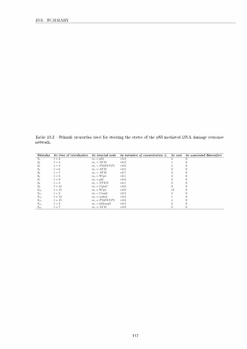
10.6. SUMMARY
Table 10.2 � Stimuli properties used for steering the states of the p53-mediated DNA damage responsenetwork.
Stimulus its time of introduction its targeted node its variation of concentration ∆c its cost its associated discomfort
S1 t = 2 mi = p53 +0.3 4 0S2 t = 4 mi = ATM +0.3 1 0S3 t = 4 mi = P53DINP1 +0.6 4 0S4 t = 6 mi = ATM +0.5 2 0S5 t = 7 mi = ATM +0.7 3 0S6 t = 8 mi = Wip1 +0.1 3 0S7 t = 9 mi = p21 +0.8 8 0S8 t = 4 mi = PTEN +0.1 3 0S9 t = 12 mi = CytoC +0.6 9 0S10 t = 15 mi = Wip1 +0.9 13 0S11 t = 2 mi = Casp3 +0.3 4 0S12 t = 13 mi = mdm2 +0.3 1 0S13 t = 15 mi = P53DINP1 +0.6 4 0S14 t = 2 mi = p53casp3 +0.3 2 0S15 t = 7 mi = ATM +0.9 3 0
147

10.6. SUMMARY
148

Chapter 11
Discussion and evaluation
Contents11.1 Introduction . . . . . . . . . . . . . . . . . . . . . . . . . . . . . . . . . . . . . 150
11.2 Logic-based modelling discussion and evaluation . . . . . . . . . . . . . . . . 150
11.3 Ontology discussion and evaluation . . . . . . . . . . . . . . . . . . . . . . . . 152
11.4 Simulation discussion and evaluation . . . . . . . . . . . . . . . . . . . . . . . 156
11.5 Optimization discussion and evaluation . . . . . . . . . . . . . . . . . . . . . 158
11.6 Summary . . . . . . . . . . . . . . . . . . . . . . . . . . . . . . . . . . . . . . . 159
149

11.1. INTRODUCTION
11.1 Introduction
In the previous chapter, we presented the experiments that have been conducted to verify and validateour contributions, the prototype CBNSimulator, its implementation and its application. This chapterproposes a discussion which aims to place our contributions in the context of similar works and to discusstheir relative advantages and disadvantages.
This chapter is divided into four sections. In the �rst section, we discuss the e�ciency of the logic-based modelling for formalizing complex biomolecular networks considering their structural, functionaland behavioural aspects. In the second section, we present an evaluation study of the semantic modellingapproach to check the ontology quality of the proposed Biomolecular Network Ontology. In the thirdsection, we discuss the performance of the proposed simulator in reproducing the behaviour and statechanges of complex biomolecular networks. And �nally, the fourth section analyses the usefulness of theoptimization approach in optimizing the transition states of complex biomolecular networks.
11.2 Logic-based modelling discussion and evaluation
With the goal of studying and simulating the dynamics of cells, various modelling techniques have beenproposed in the literature. As detailed and discussed in Chapter 2, we can �nd continuous methods such asstochastic and di�erential equations which provides good precision and are therefore powerful techniquesfor describing and modelling a speci�c problem. However, these quantitative models have also notabledisadvantages such as the fact that they require complete numerical and quantitative data (parameters,concentration levels, kinetic constants, timings, etc) which are usually unavailable or not up-to-date. Forexample, the production of structural analysis matrices in biology may require the mobilisation manyof experts over several months. Also, quantitative data can be based on an inappropriate sample, usinginadequate parameters or being misinterpreted in various ways. The excessive formalisation of thesemodels can increase the level of complexity to solve the simulation of the network. Indeed, with large-scale biomolecular networks, the quantitative model cannot be solved due to its complexity and its size.Indeed, the high number of molecular components increases the complexity of solving the di�erentialequation system modelling them.
As discussed in Chapter 2 biologists have various modelling techniques at their disposal, each withits advantages and disadvantages, depending on the desired objectives and available resources. If all thequantitative parameters are expected, a quantitative modelling is required. However, if global propertiesare the main concerns, qualitative logic-based modelling is required. A major advantage of qualitativelogic-based models is that they do not require precise quantitative data and that they are well-suited forsimulating and analysing large-scale biomolecular networks, in particular for understanding the transit-tability of complex biomolecular networks.
In the following paragraphs, we discuss the advantages and limits of the proposed logic-based mod-elling. This discussion focuses on the important logic-based modelling features, such as the modelling ofthe structure, function, behaviour of complex biomolecular networks. As well as, in the importance ofmodelling the stimuli-induced state changes.
The structural modelling The �rst step of logic-based modelling is the construction and de�nition ofthe molecular elements of the complex biomolecular networks. In this structure modelling, the essentialelements of the biomolecular networks are formalized into nodes which are categorized into genes, proteinsand metabolites. These nodes are represented either by Boolean values and real values. In fact, logicalmodels in systems biology were initially developed based on Boolean networks starting with the works ofThomas [357], Glass [358], Kau�man [18], etc. However, the proposed logic-based modelling is not totallybased on Boolean models. Indeed, in our proposed model, the nodes of the biomolecular network areformalized by Boolean variables (the case of genes which can be activated or deactivated), but also by realvariable (the case of the concentration of proteins and metabolites). Therefore, our proposed logic-basedmodelling is able to model both discrete entities, that is valued in {0; 1}, and continuous entities, whichare valued in R. This property is considered useful because it allows adding further clari�cation anddetails. Thus, the results provided by the proposed logic-based modelling, while remaining qualitative,can be �ner than those provided by the Boolean one.
Once de�ned, the nodes of the network are linked with edges. These edges represent the interaction
150

11.2. LOGIC-BASED MODELLING DISCUSSION AND EVALUATION
that can occur between each couple of nodes. Indeed, the partition of the graph nodes induces a partitioninto a range of di�erent types of interactions which allow linking the di�erent levels of the biomolecularnetwork. Thus, we conclude that the proposed logic-based modelling is a multi-level model. In fact,in a biomolecular network, interactions can occur between molecular components at the same level (forexample interactions between genes) or between di�erent levels (for example between proteins and genes)forming a complex system with multiple spatial and temporal levels. Therefore, the proposed logic-basedmodelling enable to model and integrate the experimental information that exists at di�erent levels. Thisis a hard and impossible task using quantitative models such as di�erential equations or stochastic models,because of the high number of molecular components inside the biomolecular network. In addition, thisproperty has been validated experimentally through the case studies presented in the previous chapter.All of them are composed of molecules belonging to the di�erent level and interacting with each other.
Thus, we note that the logic-based modelling is better suited for describing large-scale biomolecularnetworks, where detailed and quantitative knowledge are incomplete and where the heterogenous sub-cellular components belonging to di�erent levels of the network can be represented in a single and completeformalization.
The functional modelling In our logic-based modelling, the molecular components of the networkare not described by well-de�ned equations as in the quantitative models, but instead, rules are assignedto the participating elements to study the properties that emerge due to the interactions of the elements,usually considered as a rule-based modelling. Therefore, we note that this logic-based modelling issuitable for describing large-scale biomolecular networks with several molecular components, and arecomputationally much cheaper than the quantitative and continuous models. In addition, the proposedlogic-based modelling allows the classi�cation of the di�erent types of interactions that occur amongmolecular entities. In order to add more clari�cation about the interactions and to precise the functionof each interaction, the functional modelling of the logic-based modelling is associated with the conceptsof the Interaction Ontology proposed by Van Landeghem et al. [4]. Indeed, through this ontology, weprovide to the logic model the necessary and precise knowledge about the interactions. This additionalfeature allows to precisely de�ne the type of the interaction and the condition that activates it. Thisprecision contributes to the implementation of a valid model. This is essential for obtaining a multi-scalemodelling close to the reality and for minimizing the gaps between the proposed model and the realexperiments. We can see this precision with the modelling of the case studies. The function of eachinteraction is precise and clearly de�ned.
The behavioural modelling According to the case studies presented in the previous chapter, theproposed logic-based modelling showed its e�ciency in describing and modelling the dynamic evolutionof the biomolecular network and in reproducing its behaviour over time. This aspect is ensured by theuse of aggregation functions which compute the state transitions of the network during the simulation.Indeed, for each molecular components, we de�ne an aggregate function which computes its evolutionbased on its current state, the state of its predecessor components and the characteristics of its incominginteractions.
In our logic-based modelling, the molecular components follow simple rules (generally de�ned byexpert biologists and represented by the aggregation functions), but their interactions may induce newbehaviours (phenotypes) at the level of the network. Thus, it can be used to investigate emergentbehaviours in complex biomolecular networks. The advantage is that it can be used for networks inwhich the molecular components cannot be well de�ned by a precise mathematical equation but canbe de�ned with rules. Most importantly, they are computationally much simpler than the quantitativemodels. The limit is that it is not accurate for quantitative modelling.
Stimuli-induced state changes Complex biomolecular networks are subject to strong variationscaused by internal or external stimuli. Therefore, it is di�cult to predict their behaviour because itemerges according to their states and the state of their environment. A biomolecular network exposedto stimuli may exhibit more qualitatively di�erent behaviours than a network working without stimuli.In other words, a phase transition or a transition state can be induced by these stimuli. This aspect hasbeen considered and studied in the logic-based modelling. Most of the mathematical models presentedin Chapter 2 cannot represent and take into account these stimuli and the state changes they cause.
151

11.3. ONTOLOGY DISCUSSION AND EVALUATION
This is a very important feature that makes the di�erence from our logic-based approach to othermodels. As shown in the second and third case studies presented in the previous chapter. The proposedlogic formalism considers and models the state changes of biomolecular networks caused by stimuli.Indeed, the proposed logic-based modelling considers two types of stimuli: internal and external stimuli.In fact, the changes of a molecular state can occur either by an internal stimulus modelled by the aggregatefunction discussed above or by an external stimulus generated outside the cell. Therefore, we explicitlyde�ne this notion of stimuli as an event that causes changes in the state of the molecule on which itacts and therefore changes the state of the whole network. Then, we integrate it with the aggregationfunctions.
This point is very important and allows the logic-based modelling to understand the response of cellin the presence of external or internal stimuli, to understand drugs mode of action (through stimuli) andto predict the behaviour of complex biomolecular networks in response to drugs. This was proved by thethird case study, the p53-mediated DNA damage response network, based on this logic-based modellingthe CBNSimulator has successfully simulated and managed the transition states of the network from thenormal state to the apoptosis state and/or from the normal state to the arrest state. This case studyhighlights the fact that our logic-based modelling can be also used for modelling and understanding therelation and the mode of action between drug design and biomolecular networks modelling.
To conclude, the logic-based modelling allows biologists to produce formal models of the biomolecularnetwork of interest and then to simulate it on computers. All the properties discussed here were validatedexperimentally in the previous chapter (Chapter 10). Indeed, the case studies were formalized within thelogic-based modelling and simulated within the CBNSimulator. The �rst example network, the bacterio-phage T4 gene 32 is chosen for its simplicity, it is simple enough to be mentally computed in order to easilyjudge the produced results. However, for the other examples, we validate their modelling by comparisonwith results of other works. We conclude that the logic-based modelling provides all the elements neces-sary for formalizing and simulating the behaviours and transition states of these biomolecular networks.This logic model provides a formal and mathematical formalism to model and simulates the complexstructure of biomolecular networks, the e�ect of stimuli which target some molecular components, andthe simulation of the dynamic evolution of their behaviours.
11.3 Ontology discussion and evaluation
Ontology evaluation and validation is a very important issue to check the ontology quality. A large groupof ontology evaluation approaches exists, among those, data-driven evaluation, task-based approach,automated consistency checking, etc. [359]. Table 11.1 provides an overview of the best-known ontologyevaluation approaches and their limits. However, according to the current literature [360], there is noagreement on a methodology for validation and evaluation of ontologies. The choice of a suitable approachdepends on the purpose of evaluation, the application in which the ontology is to be used, and on whataspect of the ontology we are trying to validate and evaluate [361]. For all these reasons, we have chosen toevaluate the BNO ontology by following di�erent evaluation approaches. This choice of hybrid approachesinherits many of the advantages of each of these approaches. The goal is to evaluate our ontology in adi�erent manner. Basing on the methods presented in Table 11.1, we adopted a combination of automatedconsistency checking, expert knowledge evaluation, criteria-based evaluation, and task-based evaluationfor evaluating the BNO ontology.
Automated consistency checking The veri�cation of the logical axioms is an essential task in on-tology evaluation. Indeed, this evaluation ensures that the logical axioms are satis�able and consistent.This satisfaction consists in: (i) checking the encoding of the speci�cation, (ii) detecting errors suchas class hierarchies, redundant axioms, etc., and (iii) con�rming that the BNO ontology has been builtaccording to certain speci�ed ontology quality criteria. By de�nition, consistency checking ensures thatan ontology does not include any contradictory facts. For de�nitions to be semantically consistent, theymust be able to obtain consistent conclusions using the meaning of all de�nitions and axioms [368, 369].
To evaluate the BNO ontology and check the inconsistencies and violations of its SWRL rules, weused the latest version of the Description Logic reasoner HermiT reasoning plugin in the Protégé 5environment 1 version 1.3.8.3. HermiT can not only determine whether or not the ontology is consistent
1http://www.hermit-reasoner.com/
152

11.3. ONTOLOGY DISCUSSION AND EVALUATION
Table11.1
�Asummaryof
ontology
valid
ationevaluation
approaches.
Evaluationmethods
Description
Lim
itations
Task-basedapproach
Thisapproach
evaluatesan
ontology
byusingitin
tasksandas-
sessingtheperformance.It
isan
e�ective
approach
toassess
the
capabilityofan
ontology
toachieveitspu
rposes
andob
jectives.It
isagood
methodto
evaluate
thecapacity
anontology
toachieve
itsob
jectives
[362].
Thismethoddoes
notevaluate
the
structureofan
ontology
andignores
de�citsin
itsconceptualization.
Autom
ated
consistencycheck-
ing
Thisapproach
evaluatestheconsistencyof
anontology
byusing
Description
Logicreasoner
[363].Mostpopu
larDLreasonersare
Hermit,Pellet,Fact++,fuzzyD
L,etc.
This
method
checks
the
internal
consistencyof
anontology
(the
con-
tent
does
notcontaincontradictory
inform
ation)
and
ignore
itsback-
ground
know
ledge.
Goldstandard
checking
Thisapproach
comparesan
ontology
toagold
standard
ontology
(abenchm
arkontology)andmeasurestheirconceptualandlexical
similarities
[364].
There
may
beerrorsin
themethods
ofcomparisons
andalack
ofontol-
ogyin
thedomainof
stud
y.
Criteria-basedevaluation
Thisapproach
evaluatesan
ontology
byusingasetof
prede�ned
criteria,such
asclarity,consistency,accuracy,Com
putational
ef-
�ciency,conciseness,completeness,correctness,etc.
[365].
Somecriterialack
quantitative
mea-
suresandarefrequently
rely
onex-
pert
judgem
ent.
Datadriven
evaluation
Thisapproach
comparesan
ontology
withasource
ofdata
about
thedomainthat
isto
becoveredby
theontology
[366].
Thisapproach
cannotevaluate
the
correctnessandtheclarityof
anon-
tology.
Expertknow
ledgeevaluation
Thisapproach
evaluatesan
ontology
byusingexpert
know
ledge
who
tryto
assess
howwelltheontology
meets
asetof
prede�ned
criteria,standards,requirem
ents,etc.
[367].
This
approach
lacks
quantitative
measures.
153

11.3. ONTOLOGY DISCUSSION AND EVALUATION
but also identify subsumption relationships between concepts and resolution of the error. In terms of thetime, HermiT is as fast as other DL reasoners when classifying relatively easy-to-process ontologies, andusually much faster when classifying more di�cult ontologies. In fact, HermiT can classify a number ofontologies which no other reasoner has previously been able to handle. Using its HermiT reasoner plugin,Protégé automatically checked the inferred concepts and relations and for hierarchies, domains, ranges,and con�icting disjoint assertions. Contradictory facts and inconsistent concepts are marked with red.During the development of the BNO ontology, the automated consistency checking process was iterative.Indeed, the BNO ontology was developed incrementally by adding new de�nitions and modifying oldones. Moreover, the HermiT reasoner was used to check the correctness of the SWRL rules edited in theSWRLTab (as shown in Chapter 7). Their consistency was veri�ed by the results of our experiments asshown in Figures 7.8 and 7.9.
Figure 11.1 � Steps of the expert knowledge evaluation approach.
Expert knowledge evaluation Even if we have used best-known evaluation methods to test theconsistency of an ontology, the intervention of domain experts is always necessary, especially if a qualitylevel of the ontology is expected. The evaluation here focuses on the semantics of the BNO ontologycontent and not on its formalization. As a consequence, we proposed a method based on questionsexpressed in natural language and generated from the BNO ontology in order to test and, if necessary, tocorrect the content of the ontology using the answers that will be provided by the expert biologists. Thisquestions and answers method facilitates the task of experts. We obtained the assistance and expertiseof our collaborators from the CSTB team who have evaluated the BNO ontology and conclude that it isin accordance with their knowledge in the domain (expert knowledge).
As shown in Figure 11.1, the evaluation process consists of two steps:Fist step - Generation of questions from the content of the BNO ontology : In this step, we generate aset of questions from the ontological elements of the BNO ontology. Table 11.2 contains examples ofquestions that we have de�ned in terms of ontology elements and their translation into boolean questionsaddressed to expert biologists.
154

11.3. ONTOLOGY DISCUSSION AND EVALUATION
Second step - Evaluation of the expert's answers: In this step, we evaluate the expert's answers inorder to decide the validity of the BNO ontological elements tested or (if necessary) their modi�cationto make them valid.
We study the correlation between the number of questions generated (in terms of the number ofontological elements to be evaluated) and the size of the BNO ontology. Table 11.3 presents the number ofquestions generated according to the size of the ontologies in terms of concepts, relations and individuals.The number of questions highlights the role and the intervention of the expert biologist and its knowledgeto reduce the potential errors linked to the semantics of the content of the ontology.
The results obtained in Table 11.3 show that the number of questions generated depends on thenumber of ontological elements to be evaluated and validated.
The notion of validity in this method depends on the domain expert answering the generated booleanquestions. Thus, from our point of view, the validity of the questions corresponds to the agreementbetween the knowledge of the domain expert and the semantic content of the ontology.
Table 11.2 � An excerpt of ontological questions and their translation into Boolean questions addressedto biologists.
Questions made by an ex-
pert in ontology
Examples of its corresponding questions addressed to ex-
pert biologists
Is CLASS a type of CLASS ? Is the 'P04040 (CATA_HUMAN)' a type of 'Protein'?Is the 'G32' a type of 'Gene'?
Is INSTANCE an example ofCLASS ?
Is the 'the bacteriophage T4 G32' an example of 'Biomolecu-lar_Network'? Is the 'G32'an example of 'Gene'?
Is SUB-PROPERTY a typeof PROPERTY ?
Is the 'the catalysis' is a type of 'Interaction'?
Table 11.3 � Number of questions generated according to the size of the BNO ontology.
Concepts Properties Individuals Total Questions generated29 20 29 78 75
Criteria-based evaluation In addition to the evaluation conducted by biologists, we adopted acriteria-based evaluation method following the validation protocol proposed by Vrandecic in [365]. Thisvalidation protocol is essentially based on a number of criteria that will enable us to determine whetherour ontology is relevant or not. This protocol is based on seven evaluation criteria, (1) the accuracy, (2)the adaptability,(3) the clarity, (4) the completeness, (5) the computational e�ciency, (6) the conciseness,and (7) the consistency. We evaluate the BNO ontology against these criteria as follows.
Accuracy: The de�nitions and descriptions in the ontology agree with the expert's knowledge aboutthe �eld. The information regarding the concepts of the BNO ontology was developed from the well-known Gene ontology (GO). Moreover, we obtained the assistance and expertise of our collaborators fromthe CSTB team who have evaluated the BNO ontology and conclude that it does not contain semanticmismatches, logical inconsistencies, and conceptual con�icts.
Adaptability: We have opted for developing the BNO ontology as part of a global semantic archi-tecture composed of four ontologies that are related to each other: the Gene Ontology (GO), the SimpleEvent Model Ontology (SEMO), the Time Ontology (TO) and our development, the BNO ontology. Thisarchitecture aims at aligning and merging the BNO ontology with the rest of ontologies through equiv-alence owl:equivalenceClass or subclass owl:subclassOf relations. These relations among ontologies aredetailed in Chapter 7. This choice enhances extensibility and reusability and makes the BNO ontologyeasily adaptable to dynamical contexts.
155

11.4. SIMULATION DISCUSSION AND EVALUATION
Clarity: In developing the BNO ontology, we have been careful to assign a clear and unambiguousdescription to de�ne and categorize concepts and the relationships among concepts within our particularknowledge domain. This clarity is ensured by the use of the rdfs:comment that provides the obviouslyneeded capability to annotate an ontology. In this manner, the BNO ontology communicates e�ectivelythe intended meaning of its terms.
Completeness: This criterion measures whether the ontology can answer all the questions that itshould be able to answer. It provides an estimation of how the BNO ontology represents the domain ofthe complex biomolecular networks and their transittability. These questions were speci�ed by the expertbiologists of the CSTB team and it has been veri�ed that all of them can be answered.
Computational e�ciency: An ontology can be analysed by an inference system. In our case,the BNO ontology was treated by the two reasoning mechanisms detailed in the previous section. Weconcluded that the reasoning on the BNO ontology is consistent and allows inferences in a reasonabletime. Moreover, the complexity of this operation is adequate.
Conciseness: The terms of the BNO ontology was checked with the help of expert biologists, weassume that the ontology does not contain any redundant terms. Moreover, we have used the OntOlogyPitfall Scanner2 tool to check for logical correctness of the BNO ontology and diagnostics of ontology-design errors. Analysis results have provided great evidence of the correctness of BNO.
Consistency: This criterion ensures that the logical axioms are satis�able and consistent. Thesatisfaction of the logical axioms is recognized when it is possible to �nd a situation under which all theaxioms are true, and their consistency when it is impossible to �nd a contradiction within the axioms. Asdetailed in the previous section, reasoning in the BNO ontology was performed using an SWRL rule-basedreasonner.anisms. No inconsistencies or violations were found.
As discussed in section 11.3, there is no single best approach to evaluate an ontology. For this reason,we check the BNO ontology with di�erent approaches. Firstly, we focus in particular on automated ontol-ogy evaluation, which is a necessary precondition for the healthy development of an ontology. Automatedconsistency checking was made through the Hermit reasoner. Based on the feedback of the reasoner, in-consistencies have been corrected along the development process of the BNO ontology in an iterative way.The �nal results made by the reasoner revealed that there are no inconsistencies in the BNO ontology.The BNO ontology has been also evaluated with di�erent criteria in terms of accuracy, adaptability,clarity, completeness, etc. For each criterion, the BNO ontology is evaluated. The combination of thesecriteria allows us to check the BNO ontology from di�erent levels. The �nal results of the criteria-basedevaluation indicated that the BNO ontology was clear, extendable, and complete. Moreover, we evaluatethe usefulness of the BNO ontology through the expert knowledge evaluation. The BNO ontology wasused to model a set of case studies, among them the Bacteriophage T4 G32 case presented in this study.Results proved that the BNO ontology is able to deduce the main concepts of the case studies and theirproperties and is capable to infer new knowledge such as to compute the newt state of molecular compo-nents. These results proved that the BNO ontology is able to describe and model the transittability of abiomolecular network. However, it is important to note that the BNO ontology cannot be used directlythrough a logic reasoner to compute the transittability of large-scale networks. This would exceed thecomputing capabilities of current reasoners. Speci�c simulation tools must be designed for this task.
11.4 Simulation discussion and evaluation
The CBNSimulator is equipped with a qualitative, discrete-time simulator. This simulator allows sim-ulating in silico the behaviour of complex biomolecular networks. It simulates and tests the di�erentstate changes of biomolecular networks under various experimental conditions. The proposed qualita-tive, discrete-event simulator can also help biologists to discover and detect the stimuli that regulate thebiomolecular network such as drug e�ects to the biomolecular network.
As discussed in Chapter 4 and in the previous sections, simulation techniques can be categorized intotwo kinds: quantitative and qualitative techniques. Quantitative simulation provides the most preciseprediction in describing the behaviour of speci�c molecular entities. Nevertheless, the lack of quantitativedata limits its use with only speci�c case studies (when all the required quantitative data are available)but cannot be used in more general or large-scale networks. On the other hand, qualitative simulationsimpli�es the real simulation of the biomolecular network and is usually able to reproduce the network
2http://oops.linkeddata.es/advanced.jsp
156

11.4. SIMULATION DISCUSSION AND EVALUATION
behaviour. Moreover, this qualitative simulation can be used to explain and predict the behaviour andstate changes of the biomolecular and its components through discrete simulations.
Because of the lack of quantitative data, various qualitative simulation techniques have been proposedin the literature (see Chapter 4) however, most of them cannot support the simulation of complex andmulti-level biomolecular networks. As well as, most of them su�er from the lack of automation insimulation biomolecular properties [370].
Our proposed simulator is di�erent from the existing techniques. Indeed, it is totally based on logic-based modelling. Therefore, the power of this simulator is essentially due to the e�cient logic-basedmodelling of complex biomolecular networks which is expressive enough to integrate and capture thedi�erent elements and qualitative properties required to understand the dynamic behaviour and statechanges of biomolecular networks. But also, in the representation and the simulation of multi-levelbiomolecular networks. Thus, the proposed qualitative, discrete-event simulation is able to simulatecomplex and multi-level biomolecular networks. This property has been veri�ed through the di�erentcase studies in the previous chapter. All the case studies are composed of molecular components andinteractions belonging to a di�erent level within the biomolecular network.
In addition, our proposed qualitative, discrete-event simulation is able to perform automatic ande�cient biomolecular networks simulation. Indeed, the simulation core rests on a discrete-event basedframework (the DEVS formalism), which is used as an e�cient and accurate simulation tool of complexsystems at di�erent levels of abstraction. This ensures both synchronous and asynchronous updatingmethods for simulation. In the absence of perturbations, the simulator sets the initial states of themolecular components and the initial time, then it updates the state of all the components at the sametime. This synchronization is based on the interactions rules (aggregate functions) de�ned by the bi-ologist. It was the case of both the �rst and second case studies in the previous chapter. However,the asynchronous simulation takes into account the di�erent perturbations caused by the stimuli. Whencertain stimuli a�ect some molecular components, the simulator updated the state of these componentsthen synchronizes the state of the other components. This has experimented through the third case studyin the previous chapter.
Another important advantage of the proposed qualitative simulation mechanism is that it does notrequire precise quantitative data, but even more it can simulate the behaviour of biomolecular networksusing only qualitative data. This simulation mechanism is well-suited to simulate and analyse large-scalebiomolecular networks even with a lack of quantitative data. This proposed qualitative mechanism havebeen veri�ed and illustrated for the example of the bacteriophage T4 gene 32, as detailed in Section 8.2.3.The simulation mechanism is based on the development of a causal graph whose nodes denote variables(representing the molecular components of the network) which this simulation is concerned and edgesdenote causality relations among these variables (representing the interactions among the molecularcomponents). The state of the biomolecular network is described by a few qualitative distinct valuescorresponding to precise quantitative values (called the quantity space). To compute the qualitative valueof the nodes, this mechanism is based on both the partition rules and propagation rules. These rules areused to compute the value of the target variable at the next time t+1 based on its qualitative value at thecurrent time t and the value of its predecessors' nodes at the current time t. As detailed in Section 8.2.3,the application of the qualitative simulation to the given example shows that the proposed qualitativesimulation mechanism is able to model and simulate complex biomolecular networks, predicting theirdi�erent behaviours for di�erent simulations constraints.
To conclude, the qualitative, discrete-event simulation performed by the CBNSimulator can be usedto elucidate and predict the behaviour, state changes and properties of complex biomolecular networks.Moreover, the simulator displays the di�erent states of each molecular component in a graphic form thatis easy to interpret. We tested this simulator on the three case studies. The results show the performancesimulation of the proposed simulator in modelling and simulating complex multi-scale biomolecular net-works under di�erent environmental conditions and by considering the perturbations caused by externalstimuli.
While the proposed simulator has many advantages, it has the potential for signi�cant further im-provements. Indeed, this proposed qualitative simulation is not able to precise the di�erent time scales.This can be considered as the main limit of our qualitative, discrete-event simulation. However, we hopeto enhance our simulator by working on this point. This future direction is described in details in theperspective section of the next part. Moreover, integrating this qualitative, discrete-event simulationwith another quantitative continuous simulation tool would allow to increase the performance and obtain
157

11.5. OPTIMIZATION DISCUSSION AND EVALUATION
a semi-quantitative simulator including the advantages of both qualitative and quantitative simulations.This is one of the possible future directions for this work.
11.5 Optimization discussion and evaluation
Optimizing the transittability of complex biomolecular networks is one of the main objectives of theCBNSimulator. As discussed in 5.7.7, only a few studies have been focused on this problem and mostof them considered it as a mono-objective optimization problem and neglect other criteria for steeringthese biomolecular networks. These researches only focus on the minimization of the number of requireddriver nodes for steering the network and/or on the minimization of the number of external stimuli to beapplied on the network. However, even these two criteria are necessary conditions, they are not su�cientfor completely steering complex biomolecular networks. Indeed, this assumption is not always realistic,because steering complex biomolecular networks are in general a multi-objective optimization problem. Itrequires �nding appropriate trade-o�s among various objectives, such as the minimization of the distancebetween the simulated �nal network state and the desired network state, the minimization of the numberof external stimuli, the minimization of the cost of these stimuli, the minimization of the number of targetnodes, and the minimization of the patient discomfort.
Therefore, in this area we �rstly propose a multi-objective mathematical formulation for optimizing thetransittability of complex biomolecular networks in which we take into account more criteria such as theminimization of the distance between the simulated �nal network state and the desired network state, theminimization of the number of stimuli, the minimization of the cost of these stimuli, the minimization ofthe number of target nodes, and the minimization of the patient discomfort. Indeed, these �ve objectivesare the fundamental pillars for successfully steering the state of biomolecular networks. The �rst objectivewhich is the most important is the minimization of the distance between the simulated �nal network stateand the desired network state. This objective is ensured by the simulator and consists to compute thedistance between the obtained network and the desired network. This objective aims to provide simulatednetwork as close as possible to the desired network. The second one aims to identify the minimum numberof stimuli that are most likely to steer the global biomolecular network from the initial state to the desiredstate. In other words, this criteria aims to give priority to the quality of the external stimuli over theirquantity. The third objective is closely related to the �rst objective function and aims to minimize thetotal cost of the external stimuli to be applied to the network components. In fact, the cost of externalstimuli maybe associated with the number of external stimuli. So, if we have a number of external stimuliequal to the number of nodes and all the external stimuli have the same cost, the transittability processof the complex biomolecular network will be very expensive. That is why this criterion aims to �nd thebest compromise between the quality of the external stimuli and their cost. The fourth objective aimsto identify the minimum set of nodes to be a�ected by the external stimuli. Indeed, several studies haverevealed that, among all the nodes composing the biomolecular network, there are some speci�c nodesthat have the ability to steer the network from its actual state to another speci�c state. Moreover, thestimulation of all the nodes of the network may place the patient at risk of developing additional adversee�ects caused by the external stimuli such as ultraviolet irradiation. Thus, instead of stimulating allthe nodes randomly, it is better to have a stimulation strategy which targets a set of speci�c nodes.This will allow stimulating only a minimum number of nodes thus allowing the transition of the networkto the desired state. Then, the �fth objective aims to reduce the patient discomfort during a certaintreatment (while �nding the best compromise with the other objective functions cited previously). Inour context, the patient discomfort encompasses di�erent aspects such as patient pain, stress, vomiting,dizziness, anxiety, fatigue, etc. Indeed, the transittability of a biomolecular network can potentially beuncomfortable and negatively impacts the emotional and mental health of patients, the quality of theirlife and increases the use of health care resources. For all these reasons, we must consider this importantcriterion in the transittability process. It is important to mention that both the �rst and third objectiveshave been already used in the literature for steering biomolecular networks. However, for the second andfourth objectives, we have added them after a long discussion with expert biologists and because theyare crucial for achieving the transittability of biomolecular networks.
Moreover, we propose in Chapter 9 a two-step multi-objective optimization approach for solvingthis multi-objective problem. Our proposed approach is strongly based on the combination of bothNon-dominated Sorting Genetic algorithm (NSGA-II) to obtain the set of Pareto-optimal solutions, and
158

11.6. SUMMARY
the Technique for Order of Preference by Similarity to Ideal Solution (TOPSIS) method to provide thedecision-maker with the best compromise solution according to its preferences. The NSGA-II is one of themost widely used genetic algorithms for multi-objective problems. Thus, we think that it is interestingfor us to chose and adapt this algorithm to the problem of steering complex biomolecular networks.Based on the results obtained in Chapter 10, we conclude that the NSGA-II is well suited to solve thetransittability of complex biomolecular networks as a multi-objective optimization problem. Indeed, it isable to �nd a set of non-dominated solutions in a single run. However, even the obtained results havebeen satisfactory and positive, more can be done. In fact, we did not test our optimization problem withother methods. Maybe it is recommended to enhance the NSGA-II parameters and why not to solvethe problem with other optimization heuristics with the goal of comparing and improving the obtainedsolutions. This is remaining as future work. Moreover, it is important to note that this work of optimizingthe transittability of complex biomolecular networks is still the beginning phase in the literature. Thereare no other works treating the same problematic based on optimization tools, and there is no existingevaluation yet. We only compare our results according to the work of Wu et al. [6].
This proposed approach was tested and applied to solve the steering of the p53-mediated DNA damageresponse network with the goal of optimizing simultaneously the di�erent criteria involved in its tran-sittability, in particular, the distance between the simulated �nal network state and the desired networkstate, the number of external stimuli, their cost, the number of target nodes and the patient discomfort.We use this example because it has three states called also phenotypes, the normal, the apoptosis andthe arrest state. This case study has been already studied and simulated in the work of Wu et al. [6]and Zhang et al. [356], this allows us to compare our results by referring to their experiments. Obtainedresults are in great agreement with those of [6] and [356]. Indeed, we have succeeded in �nding thebest compromise among the di�erent criteria of the transittability and in optimizing the steering of thebiomolecular network from the normal state to one of the desired state (apoptosis or arrest state). Theexperimental results illustrate the e�ectiveness of this approach in optimizing all the objective functions.
We compare our obtained results with the most representative works proposed for steering thebiomolecular networks using the controllability notion in literature. We note that the proposed approach(in agreement with Wu et al. [6] results) proposes to a�ect the minimum set of nodes (not all nodes)rather than the entire nodes of the biomolecular networks. As a consequence, the proposed approachprovides less external stimuli than the total number of the network nodes and consequently, the totalcost of these stimuli will certainly be less costly than the use of controllability notion [28]. In addition,the proposed method considers as another objective the minimization of the patient discomfort. Thisincreases the applicability of translational medicine for improving human health and disease, includinggenetic and environmental factors of patient's well-being. This is a great opportunity to understanddiseases and �nd new diagnoses and treatments. Therefore, applications of the proposed optimizationapproach can be used in the design of treatments such as chemotherapy, the identi�cation of potentialdrug targets in a signalling network of human cancer, or to study the phenotype transitions (for example,to direct a biomolecular network from its abnormal or disease phenotype to a healthy phenotype).
11.6 Summary
In this chapter, we have presented a discussion of our four proposed approaches. These approaches arecombined together under the CBNSimulator platform. This platform enables the study of the behaviour ofcomplex biomolecular networks through the creation of their logic modelling. As seen with the three casestudies, the logic-based modelling provides all the necessary elements to model biomolecular networks.This logical formalism treats the biomolecular network based on three aspects: the structural, functional,and behavioural modelling of the network. Furthermore, with the goal of enriching this logic-basedmodelling, the CBNSimulator integrates a semantic level to this logic modelling through the semanticmodelling. This semantic modelling aims to enrich and infer new knowledge, to detect more propertiesand relationships among the molecular components, and to suggest new inferring data in order to providethe logic model with complementary knowledge and data. This semantic approach joined to the logic-based modelling provides a powerful formalism for modelling and representing complex biomolecularnetworks. Moreover, the CBNSimulator provides a qualitative, discrete-event simulator. This simulationapproach was used to elucidate and predict the behaviour, state changes and properties of the threecase studies. Simulation results were displayed in a graphic form to facilitate their interpretation and
159

11.6. SUMMARY
analysis. Finally, the CBNSimulator proposes an optimization module allowing biologists to steer complexbiomolecular networks from their actual state to another speci�c state. The experimental results illustratethe e�ectiveness of this approach in optimizing simultaneously the di�erent criteria involved in theirtransittability, in particular, the distance between the simulated �nal network state and the desirednetwork state, the number of external stimuli, their cost, the number of target nodes and the patientdiscomfort. Thus, using the CBNSimulator, biologists can perform in silico experiments, in particular,the steering of the biomolecular network from a state to another one, which has the advantage of beingless costly in time and resources than the in vitro and in vivo experiments. However, this platform mustcontinue to be re�ned and enhanced. Interesting research directions are discussed in the next part.
160

General conclusion and future research
In this part, we conclude by brie�y foregrounding our thesis' contributions, and suggest speci�c openquestions and directions for future research.
Conclusion
An important objective of systems biology is the construction of predictive models for understanding thedynamic behaviour of complex biomolecular networks and their transittability. Indeed, existing studieshave focused mainly on numerical models involving (highly non-linear) di�erential equations and usingtools for estimating parameters [371] to formalize and simulate biomolecular networks. However, asdiscussed in Chapter 2 to Chapter 4 state-of-the-art quantitative models cannot be reused or mergedwith other models in a systematic fashion, and are limited to a small number of variables [371].
Moreover, with the recent development of high-throughput technologies, huge amounts of data havebeen generated to describe the complex processes and molecular mechanisms at work in the cell, throughthe study of cellular components on several levels.
With these advances, systems biology faces numerous novel challenges:
• The �rst challenge is how to extract important knowledge from all this data in order to understandand infer cellular functions and behaviours in di�erent conditions.
• Another challenge is the modularity of complex biomolecular networks. It is not an easy task tomodel and combines large-scale genomic, proteomic and metabolic data in order to obtain a mixedmodel of the complex biomolecular network. This is a restriction to the re-use of models in systemsbiology because they are implemented for a speci�c context.
• An important challenge is to simulate the behaviour of biomolecular networks using logic andqualitative models to automate various forms of biological reasoning. Indeed, understanding thetransition states of biomolecular networks and drug target discovery, require qualitative tools toassist the biologist when certain numerical data are unavailable.
• Another challenge for systems biology is to enrich existing quantitative models to include precisesemantics of biomolecular networks behaviour and build formal methods to reason about them.
• A supplementary important challenge is to understand the dynamic aspects of these biomolecularnetworks in order to control and guide their behaviour. This issue is known through the "transitta-bility" that focuses on the idea of steering the complex biomolecular network from an unexpectedstate to a desired state.
To address these challenges, the overall goal of this study is to propose an intelligent platform thatenables biologists to simulate the state changes of biomolecular networks with the goal of steering theirbehaviours. The development of such a platform involves several related computing methods belonging todi�erent domains such as mathematical systems modelling, knowledge engineering, computer simulation,and combinatorial optimization. Thus, the intelligence of our platform derives from the combination ofdiverse techniques and �elds of study. The �rst element of intelligence is presented in this dissertationthrough the logic-based modelling approach that addresses the problem of modelling complex biomolec-ular networks considering the diversity and heterogeneity of their molecular components, and adoptinga global vision which considers their multi-level aspects. This formalization focuses on the structure ofthe network (modelling of the diverse components and their interactions), network control (identi�cation
161
General conclusion and future research
of the function and role of each component) and network dynamics (observation of its behaviour overtime). The second feature of our intelligent platform concerns the semantic approach, which provides thenecessary knowledge for modelling and understanding the behaviour of complex biomolecular networksand their state changes. The Biomolecular Network Ontology presented in this dissertation formalizesthe domain knowledge of complex biomolecular networks making it visible and accessible to all biologistsworking on this topic. Moreover, the reasoning and simulation system exploits all this formally encodedknowledge in order to reproduce the behaviour of complex biomolecular networks and their componentsover time even with incomplete knowledge. Finally, the proposed multi-objective optimization approachtake into account several criteria, such as: the minimization of the distance between the simulated �nalnetwork state and the desired network state, the minimization of the number of stimuli, the minimizationof the cost of these stimuli, the minimization of the number of target nodes, and the minimization of thepatient discomfort, for optimizing the transittability of complex biomolecular networks.
Contributions
We recall our four contributions here. For each contribution, we stress the results and general conclusions.More general perspectives of our contributions are left to the next section.
In Chapter 6, we propose a logic-based formalization which allows biologists to model the di�erentelements that compose a complex biomolecular network, and to identify and categorize all its componentsand the nature of their interactions. Indeed, the logic-based formalization was tested with di�erent casestudies and provides a relatively simple modelling approach able to capture interesting and relevantbehaviours in the cell. In particular, in the case of the poorly understood biomolecular network wherequantitative data and parameters are often scarce and hard to obtain. However, to obtain an optimaland more realistic modelling, we need to enhance it with an additional semantic layer. For this reason,we propose a semantic architecture for providing and inferring more knowledge about the functioning ofcells at a molecular level.
The proposed semantic architecture (Chapter 7) consists of four ontologies: three of them alreadyexist in the literature, the Gene Ontology (GO), the Simple Event Model Ontology (SEMO), the TimeOntology (TO) and we are developing the Biomolecular Network Ontology (BNO). Linked together, theseontologies provide the necessary concepts for modelling the dynamic behaviour and the transition statesof a complex biomolecular network. The Biomolecular Network Ontology describes the static structureof the biomolecular network. Merging with the Simple Event Model Ontology, the Biomolecular NetworkOntology describes what can carry out each component of the biomolecular network and the conditionsfor these activities. Finally, the Biomolecular Network Ontology, the Simple Event Model Ontology andthe Time Ontology describe how the biomolecular network and its individual components evolve overtime.
In the same chapter, we focus on the implementation of the BNO ontology to describe the domainknowledge of complex biomolecular networks in their static state. This ontology provides informationon the biomolecular network and its components (nodes, interactions, states, transition states, etc.) andan indication of the network's context such as the type of sub-network, the type of node, the conditionsand nature of interactions, etc. This allows to precisely explain and interpret the semantic context inorder to achieve intelligent modelling of biomolecular networks and their state changes. These statechanges can be computed with a rule-based system using OWL-SWRL rules. These rules represent a"proof of concept" demonstrating the logical consistency of the approach and validating the relevanceof the ontology. Additionally, we simulate the evolution of di�erent biomolecular networks. Obtainedresults are encouraging and indicated that the BNO is consistent, credible and e�ective in describingrelevant knowledge required in understanding the behaviour of complex biomolecular networks and theirstate changes. Nevertheless, more e�cient simulation tools should be used to study larger biomolecularnetworks.
Moreover, it is important to note that the complexity of biomolecular networks is �rstly due to theirlarge number of coupled components, but also to the diversity of these molecular components and to theirintricate interactions. Indeed, biomolecular networks consist of various subnetworks which themselves arecomposed of several molecular components interacting in their turn with each other, producing a complexglobal behaviour. The complexity and large size of these networks have prevented a fully quantitativesimulation. Thus, biologists require tools allowing them to gain insights into the behaviour of complex
162

General conclusion and future research
biomolecular networks by simulating the di�erent states of their components over time.Therefore, we propose a qualitative, discrete-event simulation in Chapter 8. The qualitative simulation
predicts the set of possible states based on the logic-based modelling of the real network. The linkbetween the logic model and the qualitative simulation is ensured by the partition and propagation rules.The value of the qualitative simulation comes from the ability to describe natural types of incompletenumerical knowledge, and the ability to deduce a complete set of possible states (using qualitative valuesrather than real numbers). We chose to use qualitative reasoning for two reasons: (i) To understand theoverall functioning and properties of complex biomolecular networks through the analysis and simulationof the dynamical model, and the interpretation of the obtained qualitative knowledge. (ii) To steer thesenetworks by allowing to evaluate their simulation at any time, even in the lack of quantitative knowledge.
In addition to the qualitative simulation, we propose a discrete-event simulation. This approach wasinspired by the DEVS formalism [339], a formalism for supporting the modelling of complex systems,and based on the logic-based modelling. This simulation allows biologists to analyse and predict thee�ect of changes, the behaviour of the biomolecular network components. It also enables the study of theinternal interaction of a subsystem with a complex system. This approach aims at providing biologistswith a �exible tool for simulating biomolecular networks by reproducing their behaviour and the stateof their components over time and consequently allows them to analyse and understand simulated cellphenomena. These approaches have been veri�ed on diverse biomolecular networks, and the simulationresults obtained were formally treated and validated by expert biologists. Indeed, these results correspondto their domain knowledge.
The computation of the transittability of complex biomolecular networks can be considered as anoptimization problem. As discussed in Chapter 5, only a few studies have been carried out for thisproblem and most of them have focused only on the minimization of the nodes required to steer theentire network and on the minimization of the number of stimuli to be applied on the network. However,this assumption is not always realistic, because steering complex biomolecular networks are in general amulti-objective optimization problem. It requires �nding appropriate trade-o�s among various objectives,for example between the appropriate nodes to be stimulated and the number of external stimuli to beused, their cost and the patient discomfort.
Consequently, we propose (in Chapter 9) a multi-objective mathematical formulation for optimizingthe transittability of complex biomolecular networks in which we take into account more criteria suchas the minimization of the distance between the simulated �nal network state and the desired networkstate, the minimization of the number of stimuli, the minimization of the cost of these stimuli, theminimization of the number of target nodes, and the minimization of the patient discomfort. Moreover,we propose a two-step multi-objective optimization approach for solving this multi-objective problem.Our proposed approach is strongly based on the combination of both Non-dominated Sorting GeneticAlgorithm (NSGA-II) [340] to obtain the set of Pareto-optimal solutions, and the Technique for Orderof Preference by Similarity to Ideal Solution (TOPSIS) method [341] to provide the decision-maker withthe best compromise solution according to its preferences.
In order to validate all these methods proposed in Chapter 6, 7, 8, and 9, the prototype CBNSimulatorhas been developed in Chapter 10. The overall architecture of CBNSimulator is composed of four modules.Each module corresponds to one of the proposed approaches discussed above. As well as, we haveapplied all these approaches to various biomolecular networks, among them the autoregulation of thebacteriophage T4 gene 32, the phage lambda and the p53-mediated DNA damage response network.The logic-based modelling approach provides all the elements that we need to understand the structure,function and behaviour of these case studies, but also to study its evolution over time. In addition, theproposed semantic approach produces good quality (e�cient) simulation and rapid reasoning of thesebiomolecular networks behaviour. The SWRL reasoner is able to reproduce the overall behaviour ofthese biomolecular networks induced by the SWRL rules de�ned by the expert biologists. It reproducesbehaviours similar to those observed in real life. Indeed, the qualitative simulation method providesall possible simulation results of the given networks and their molecular components. Thus, based onthis qualitative method, it is possible to predict the behaviour of these networks even in the absenceof quantitative information. It is su�cient to have some essential information to predict their futurebehaviour. Moreover, the proposed multi-objective optimization approach for solving this multi-objectiveproblem takes into account di�erent criteria which are important to study the transittability of complexbiomolecular networks. It provides a set of optimum solutions to the problem according to the userpreferences. The results obtained from this study are encouraging and it is expected that they will
163

General conclusion and future research
be useful in understanding the behaviour of complex biomolecular networks and in optimizing theirtransittability.
However, our proposed CBNSimulator has some important limitations. First, the complexity of realbiomolecular networks means that a number of simpli�cations are necessary. For example, we have notincluded interactions between metabolites and genes, although it is known that speci�c metabolites, suchas nicotine, do interact directly with genes. Second, in order to completely understand biomolecularnetworks, some quantitative aspects should be taken into account. To address this, the quantitativemethods described in the State-of-the-art could be used in combination with our tool. Third, the casesstudies used here are relatively small and medium-sized networks, and in fact, our semantic methodcannot simulate very large networks. The main reason is the time constraint and the exponential numberof interactions among the molecular components. It is di�cult to compute the dynamics of all theinteractions at the same time. For this reason, we integrate a framework for dynamic simulation ofcomplex biomolecular networks based on the Discrete Event System Speci�cation (DEVS) formalism[339], which allows the description of biomolecular networks at di�erent levels. In order to validate allthese methods proposed in Chapter 6, 7, 8, and 9, the prototype CBNSimulator has been developedin Chapter 10. The overall architecture of CBNSimulator is composed of four modules. Each modulecorresponds to one of the proposed approaches discussed above. As well as, we have applied all theseapproaches to various biomolecular networks, among them the autoregulation of the bacteriophage T4gene 32, the phage lambda and the p53-mediated DNA damage response network. The logic-basedmodelling approach provides all the elements that we need to understand the structure, function andbehaviour of these case studies, but also to study its evolution over time. In addition, the proposedsemantic approach produces good quality (e�cient) simulation and rapid reasoning of these biomolecularnetworks behaviour. The SWRL reasoner is able to reproduce the overall behaviour of these biomolecularnetworks induced by the SWRL rules de�ned by the expert biologists. It reproduces behaviours similarto those observed in real life. Indeed, the qualitative simulation method provides all possible simulationresults of the given networks and their molecular components. Thus, based on this qualitative method, itis possible to predict the behaviour of these networks even in the absence of quantitative information. Itis su�cient to have some essential information to predict their future behaviour. Moreover, the proposedmulti-objective optimization approach for solving this multi-objective problem takes into account di�erentcriteria which are important to study the transittability of complex biomolecular networks. It providesa set of optimum solutions to the problem according to the user preferences. The results obtained fromthis study are encouraging and it is expected that they will be useful in understanding the behaviour ofcomplex biomolecular networks and in optimizing their transittability.
However, our proposed CBNSimulator has some important limitations. First, the complexity of realbiomolecular networks means that a number of simpli�cations are necessary. For example, we have notincluded interactions between metabolites and genes, although it is known that speci�c metabolites, suchas nicotine, do interact directly with genes. Second, in order to completely understand biomolecularnetworks, some quantitative aspects should be taken into account. To address this, the quantitativemethods described in the State-of-the-art could be used in combination with our tool. Third, the casesstudies used here are relatively small and medium-sized networks, and in fact our semantic methodcannot simulate very large networks. The main reason is the time constraint and the exponential numberof interactions among the molecular components. It is di�cult to compute the dynamics of all theinteractions at the same time. For this reason, we integrate a framework for dynamic simulation ofcomplex biomolecular networks based on the Discrete Event System Speci�cation (DEVS) formalism[339], which allows the description of biomolecular networks at di�erent levels.
Suggested future work
Our contributions detailed in the previous section suggest some speci�c open questions and directions forfuture research. The remainder of this section will lay out some of these perspectives. Indeed, althoughthe dynamic synchronization among the four modules (corresponding to our contributions): logic-basedmodelling, semantic approach, qualitative and quantitative simulation, and the multi-objective optimiza-tion module to achieve the full development of our intelligent platform, the CBNSimulator, there are stillsome important improvements that can be made in further researcher.
• About our �rst contribution:
164

General conclusion and future research
As mentioned in the previous section, our proposed logic-based modelling does not include interactionsamong metabolites and genes, although it is known that some speci�c metabolites, such as nicotine, dointeract directly with genes. One possible direction to explore is to extend the logic-based modelling withthe goal of integrating and considering this hypothesis.
• About our second contribution:
An interesting question which we are currently investigating is the problem of extending the semanticapproach presented in this thesis by applying it to large and concrete biomolecular networks and enhancingits performance in order to apply it in the domain of drug discovery. This can be solved by integratingother ontologies and adding them to our semantic approach. Considering that SWRL rules providepowerful solutions for problems that cannot be solved with standard Description Logic-based reasoning,we plan to provide a user interface (by adding a functionality to the CBNSimulator) that allow biologiststo de�ne their speci�c SWRL rules to represent their preferences and take pro�t of the knowledge requiredfor speci�c and personalized application.
• About our third contribution:
The components of the biomolecular network and their interactions are physically and temporallyorganized to ensure the production of a particular behaviour or phenotype. These spatiotemporal aspectsare important to understand the functioning of a cell as a whole. The spatial organization of the networkincludes the location of the di�erent molecular components as well as their positions and levels (proteomic,metabolic, etc.). The temporal organization includes the order of the sequence of state transitions ofeach component, the duration and frequency of these interactions. Both of these spatiotemporal aspectsconstitute the dynamic properties of the biomolecular network. In this work, to maintain simplicity wetake into account the multi-level aspect of the network (considering the di�erent levels of the biomolecularnetwork), but we do not consider the di�erent biological time levels. Indeed, the timing of processeslevels with size: from nanosecond at the level of single molecules to microseconds at the level of proteinsinteraction, to hours at cellular processes, etc. We neglect this property and work within a �xed timelevel. To address this limitation, we must include our modelling with a timing generator that allows tofollow the dynamics of the system and change among di�erent time levels according to the given spatiallevel and the nature of the process. Moreover, to overcome these di�culties of time levels, a simulatorbased on agent-based systems may be proposed because they take into account the e�ects of di�erenttime levels.
• About our fourth contribution:
The transittability of complex biomolecular networks has di�erent perspectives in terms of optimiza-tion criteria (minimization of total transittability time and other objectives), therefore, it will be interest-ing to improve and detail some objectives such as the patient comfort. Moreover, we plan to improve theperformance of our NSGA-II algorithm by implementing a hybridisation with a local search algorithm,such as the Nelder-Mead simplex method, and compare its performance with other meta-heuristics inorder to improve the computation time of our optimization algorithm and the quality of the solutions.We can also use the EASEA platform3 (EAsy Speci�cation of Evolutionary Algorithms) that ensuresthe parallel implementation of genetic algorithms on a computer network furnished with GPGPU cards(General-Purpose computation on Graphics Processing Units). Using this platform we can solve thetransittability of complex and large-scale networks by taking the advantages of the massive parallelismof many-core architectures.
• About the prototype CBNSimulator:
Our prototype, the CBNSimulator, needs to be improved. First, we are actually working to make amore dynamic synchronization among the four modules, the logic-based modelling, semantic approach,qualitative and quantitative simulation, and the optimization module to improve the performance of ourplatform. As well as, we plan to extend the experiments in order to assess and analyse in more detailthe impact of our di�erent proposals. Indeed, simple cases studies are not enough to completely evaluate
3http://easea.unistra.fr/index.php/EASEA_platform
165

General conclusion and future research
and validate our approaches, therefore, new experiments could be carried out within the applicationof the CBNSimulator. Moreover, the CBNSimulator platform currently o�ers only the simulation andoptimization layer for complex biomolecular networks. The logic and semantic modelling modules havebeen implemented implicitly in the code and speci�cally for each example. Thus, we plan to add newinterfaces allowing the user to de�ne and explicitly design the logical and semantic modelling of his ownbiomolecular network. Solving these problems will contribute to the generality of our platform.
166

Detailed abstract in French
La biologie des systèmes représente un nouveau domaine de la biologie qui pourrait avoir des applicationsimportantes en recherche biomédicale et en ingénierie biologique. En e�et, ce domaine académiquevise à proposer des modèles de fonctionnement intégrant di�érents niveaux d'informations pour décrireet comprendre le comportement d'une cellule, représentée par un réseau biomoléculaire complexe. Encombinant les données biologiques expérimentales et les techniques de l'informatique, la biologie dessystèmes o�re la possibilité d'avoir une vraie compréhension du fonctionnement et des interactions entreles di�érents composants moléculaires d'une cellule à tous les niveaux de son organisation (génétique,protéomique et métabolique).
En e�et, la cellule peut être considérée comme un système complexe composé de milliers d'entitésmoléculaires di�érentes (gènes, protéines et métabolites), qui interagissent physiquement, fonctionnelle-ment et logiquement créant un réseau moléculaire. Pour réduire la complexité de ce réseau, la plupartdes études traditionnelles se sont concentrées uniquement sur un niveau particulier du système cellu-laire, comme les réseaux de régulation des gènes, les réseaux d'interaction protéine-protéine ou encore lesréseaux métaboliques. Diverses approches ont été développées pour modéliser, analyser et comprendreces réseaux, y compris les équations di�érentielles ordinaires, les méthodes stochastiques, les réseauxbooléens, les réseaux bayésiens, les réseaux de Petri, etc. et des études comparatives de ces techniquesont été réalisées. Néanmoins, peu d'approches ont été développées pour étudier le système cellulaire dansson ensemble, et en particulier les interactions entre les di�érents types de réseaux moléculaires. De plus,la plupart des techniques de modélisation existantes ne tiennent pas compte de l'évolution dynamique duréseau ainsi que de ses di�érentes transitions d'états.
Récemment, certains auteurs ont commencé à aborder les aspects dynamiques et ont introduit desconcepts tels que la "contrôlabilité" d'un réseau, où la capacité de diriger un réseau complexe d'un étatinitial vers un autre état désiré est mesurée par le nombre minimum de n÷uds pilotes requis (n÷udsayant la capacité de diriger l'ensemble du réseau). Ils ont montré que pour avoir une contrôlabilitécomplète, le nombre minimum de n÷uds pilote est de 80 % des n÷uds d'un réseau biomoléculaire. Cerésultat a conduit d'autres groupes à développer un cadre théorique pour étudier les transitions entredeux états spéci�ques de réseaux complexes, un concept qu'ils appellent la " transitabilité " du réseau.Cette transitabilité exprime l'idée de pouvoir piloter un réseau complexe d'un état initial vers un autreétat désiré en stimulant un minimum de n÷uds.
Notre thèse s'inscrit dans ce contexte. Par conséquent, nous proposons une plate-forme qui permetaux biologistes de simuler les changements d'état des réseaux biomoléculaires dans le but de piloter leurscomportements et de les faire évoluer d'un état non désiré vers un état souhaitable. Cette plate-formeconsidérée comme un système intelligent combine la modélisation logique, le raisonnement sémantiqueet qualitatif, un outil de simulation et un algorithme d'optimisation. Ses objectifs généraux sont: Car-actériser les composants moléculaires d'une cellule; Comprendre les interactions dynamiques entre lescomposants moléculaires et les stimuli environnementaux; Fournir un outil aux biologistes pour repro-duire le comportement de réseaux complexes; et Déduire un ensemble optimal de stimuli externes àappliquer pendant un intervalle de temps prédéterminé pour piloter le réseau de son état actuel à un étatdésiré.
Ainsi, cette plate-forme, que l'on a intitulé CBNSimulator, o�re aux biologistes la possibilité de (i)modéliser et simuler un réseau biomoléculaire complexe en se basant sur le modèle logique qui est décritsémantiquement par une modélisation sémantique, et (ii) guider et piloter la transition de ces réseauxde leur état actuel à un état souhaité dans des conditions spéci�ques et contrôlées. CBNSimulator estcomposée de quatre modules: un module de modélisation logique, un module ontologique, un module desimulation et un module d'optimisation.
167

Detailed abstract in French
1. Le module de modélisation logique: Ce module représente le point de départ de tout nouveauréseau biomoléculaire dé�ni par l'utilisateur. Cette modélisation logique a été conçue pour fournirtous les éléments nécessaires à la modélisation du réseau biomoléculaire en tenant compte de sesdi�érents niveaux et composants moléculaires. Par exemple, l'utilisateur peut spéci�er la liste descomposants moléculaires et leur type, la liste des interactions entre ces composants et les conditionsqui les activent, etc. Cette modélisation logique tient compte de la complexité et de l'hétérogénéitéde ces composants moléculaires et de leurs structures multi-niveaux.
2. Le module ontologique: Ce module assure la gestion, la modélisation et le partage des connaissancesdes experts biologistes. Ce module prend en entrée toutes les informations natives introduites parl'expert (état du réseau, sa structure, etc.) à travers la modélisation logique fournie par le premiermodule. Ensuite, le module ontologique fournit, en sortie, un réseau composé de connaissancesnatives et déduites (inférées). Ce module joue un rôle très utile pour l'enrichissement de la formal-isation du réseau, surtout lorsque la modélisation logique du réseau manque de détails. De plus,les informations supplémentaires fournies par ce module peuvent être utilisées pour identi�er denouvelles relations potentielles entre les composants moléculaires du réseau.
3. Le module de simulation: Ce module permet aux utilisateurs de simuler et/ou de reproduire lecomportement dynamique du réseau. En e�et, ce simulateur intègre toutes les informations fournitpar l'expert (le réseau enrichi de connaissances natives et inférées) avec d'autres paramètres a�n demieux reproduire le comportement du réseau biomoléculaire et de ses composants dans le temps.Les résultats générés lors de la simulation sont a�chés à l'utilisateur sous forme graphique a�n defaciliter leur interprétation, et peuvent également être transmises au module d'optimisation.
4. Le module d'optimisation: Ce module fournit un moyen de diriger et piloter le réseau de sonétat actuel vers un autre état spéci�que. Cette optimisation est réalisée en spéci�ant les étatsinitial et souhaité du réseau, ainsi que tous les stimuli externes possibles dé�nis par l'utilisateur.Ensuite, ce module d'optimisation fournit les meilleures séquences de stimuli pour piloter le réseaubiomoléculaire de son état initial à l'état désiré et, en�n, présente les résultats en fonction despréférences de l'utilisateur. Ce module permet également d'optimiser la transitabilité du réseau enminimisant divers critères, tels que: la distance de proximité entre l'état du réseau obtenu à la �nde la simulation et l'état du réseau désiré, le nombre de stimuli externes, leur coût global, le nombrede n÷uds cibles et l'inconfort du patient.
Le manuscrit de thèse est divisé en trois parties et est composé de onze chapitres. Les parties "Étatde l'art" et "Contributions" ont été divisées chacune en quatre chapitres en fonction des modules del'architecture de la plate-forme proposée. La première partie Etat de l'art vise d'abord à présenterl'environnement biologique dans lequel nous travaillons en explorant l'histoire conceptuelle de la biologiedes systèmes et en dé�nissant ses principaux concepts. Ensuite, à présenter les di�érents outils et ap-proches qui ont été proposés dans les di�érents domaines de recherche couverts par cette thèse. À la �n dechaque chapitre, une section est consacrée à la dé�nition de l'énoncé du problème lié à chaque domaine derecherche spéci�que. Le premier chapitre présente l'environnement biologique et le contexte dans lequelnous travaillons. Nous nous concentrons principalement sur les réseaux biomoléculaires complexes et leurtransitabilité. Le deuxième chapitre capitalise les notions de base des modèles mathématiques en biologiesystémique, synthétise les plus importants d'entre eux, et présente la principale problématique abordéepar notre thèse dans ce domaine: une modélisation logique des réseaux biomoléculaires complexes. Letroisième chapitre donne un aperçu sur les ontologies, décrit les principales bio-ontologies qui ont étéproposées en biologie des systèmes et présente la principale problématique abordée par notre domaine:une ontologie de domaine pour décrire le domaine des réseaux biomoléculaires complexes. Le quatrièmechapitre se focalise sur les notions de base de la simulation en biologie des systèmes, détaille les principauxoutils et plates-formes de simulation dans la littérature, et présente la principale problématique abordéepar notre thèse dans ce domaine: un simulateur qualitatif et à événements discrets pour comprendre lecomportement des réseaux biomoléculaires complexes. En�n, le dernier chapitre de cette partie présenteles connaissances de base sur les outils d'optimisation, y compris une synthèse des travaux menés sur lesproblèmes d'optimisation en biologie des systèmes, et présente la principale problématique abordée parnotre thèse dans ce domaine: un algorithme génétique pour résoudre et optimiser la transitabilité desréseaux biomoléculaires complexes.
168

Detailed abstract in French
Après avoir présenté le contexte et l'état d'avancement de nos travaux dans la première partie dece manuscrit, la deuxième partie Contributions est consacrée à nos contributions sur la conception etle développement d'une plate-forme de simulation des changements d'état de réseaux biomoléculairescomplexes dans l'espoir de comprendre et de piloter leur comportement. Cette plate-forme se compose dequatre modules de base: (i) le module de modélisation pour formaliser le comportement dynamique desréseaux biomoléculaires, (ii) le module ontologique pour fournir une description riche des entités cellulaireset les interactions ayant lieux entre elles, (iii) le module de simulation pour reproduire le comportementdynamique des composants de chaque réseau dans le temps et (iv) le module d'optimisation pour fournirun ensemble de stimuli externes proposant le meilleur pilotage du réseau biomoléculaire d'un état donnéà un autre. Ces contributions sont organisées par domaine spéci�que. Ainsi, selon chacun des modulesde l'approche que nous proposons, quatre contributions ont été apportées à ce travail. C'est pourquoicette partie est divisée en quatre chapitres, chacun présentant nos contributions dans un domaine derecherche spéci�que. Le sixième chapitre propose une approche logique pour modéliser le comportementdynamique des réseaux biomoléculaires. Ce formalisme s'appuie sur les trois niveaux d'analyse dé�nispar la théorie des systèmes: la modélisation structurelle, fonctionnelle et comportementale. En e�et, ilvise à décrire et à analyser toutes les propriétés et les mécanismes des réseaux biomoléculaires complexes.Cette modélisation basée sur la logique constituera l'élément de base pour la modélisation, la simulationet la compréhension de la transitabilité de ces réseaux complexes. Le septième chapitre présente uneapproche sémantique pour la modélisation des réseaux biomoléculaires et décrit l'implémentation de laBiomolecular Network Ontology (BNO), une ontologie créée spécialement pour répondre aux besoinsde l'analyse du comportement des réseaux biomoléculaires complexes. Cette ontologie fournit une basepour la simulation qualitative de ces réseaux. Le huitième chapitre propose deux types de simulation:une simulation qualitative et une simulation à événements discrets. La première répond à la complexitédu calcul des méthodes de simulation quantitative qui sont parfois impossibles à mettre en ÷uvre. Ladeuxième méthode est une simulation intégrative à événements discrets qui considère que le comportementdu réseau biomoléculaire complexe émerge de l'interaction des di�érents niveaux du réseau. En�n ledernier chapitre de cette partie, présente tout d'abord une formulation mathématique multi-objectifspour optimiser la transitabilité des réseaux biomoléculaires complexes considérant divers critères telsque la minimisation de la distance de proximité entre l'état du réseau obtenu à la �n de la simulationet l'état du réseau désiré, la minimisation du nombre de stimuli externes, la minimisation de leur coûtglobal, la minimisation du nombre de n÷uds cibles, et la minimisation de l'inconfort du patient. Cechapitre présente également une approche d'optimisation multi-objectifs pour résoudre ce problème. Cetteapproche est basée sur la combinaison de l'algorithme génétique de tri non dominé (NSGA-II) qui génèrel'ensemble des solutions optimales de Pareto-optimal, et de la méthode TOPSIS (Technique for Order ofPreference by Similarity to Ideal Solution) pour fournir au décideur la meilleure solution de compromisen fonction de ses préférences.
La troisième partie Validation présente, détaille et discute nos résultats. Cette partie est divisée endeux chapitres. Le dixième chapitre qui présente un prototype de plate-forme, intitulé CBNSimulator,que nous avons développé pour valider nos contributions ainsi que les expériences que nous avons menéespour déterminer les performances de ce prototype. Cette plate-forme est basée sur le modèle logique etsémantique du réseau biomoléculaire ainsi que sur les performances de simulation à événements discretspour comprendre l'évolution et le comportement des réseaux biomoléculaires complexes dans le temps.Le onzième et dernier chapitre discute les résultats des diverses expériences que nous avons menées a�nd'évaluer nos contributions, tout en comparant nos résultats à ceux de la littérature.
Ainsi pour résumer, cette thèse présente quatre contributions:En première partie, nous proposons une approche de modélisation logique permettant de décrire et
modéliser les réseaux biomoléculaires complexes. Cette modélisation logique se base sur la séparationdes trois axes de la théorie des systèmes, à savoir: l'aspect structurel, fonctionnel et comportemental duréseau. Cette séparation des connaissances de nature di�érente simpli�e la complexité de la tache demodélisation des réseaux biomoléculaires complexes.
Par la suite, une deuxième contribution porte sur une approche sémantique composé de quatre on-tologies, Gene Ontology, Simple Event Ontology, Time ontology et Biomolecular Network Ontology.Conjointement, ces ontologies permettent d'enrichir la modélisation logique des réseaux biomoléculairesen rajoutant une couche sémantique fournissant les concepts nécessaires à la modélisation du comporte-ment dynamique et des états de transition d'un réseau biomoléculaire complexe. En particulier, nousavons développé la Biomolecular Network Ontology (BNO) pour décrire les connaissances du domaine
169

Detailed abstract in French
des réseaux biomoléculaires complexes et fournir toutes les connaissances et les éléments nécessaires àla réalisation d'une modélisation intelligente des réseaux biomoléculaires et de leurs changements d'état.Ces changements d'état sont simulés grâce à un système de raisonnement à base de règles SWRL.
En troisième partie, nous présentons une simulation qualitative à événements discrets, basée sur lamodélisation logique et sémantique, pour simuler qualitativement le réseau biomoléculaire et interpréterson comportement (ainsi que celui de ses di�érents composants moléculaires) dans le temps. Cettetechnique de simulation facilite la compréhension, l'analyse et l'interprétation du fonctionnement globalet des propriétés des réseaux biomoléculaires complexes. Elle permet également de simuler ces réseauxen permettant d'évaluer leur état à tout moment, même en cas d'absence de connaissances quantitatives.
Finalement, dans la quatrième contribution nous proposons une formulation mathématique multi-objectifs pour optimiser la transitabilité des réseaux biomoléculaires complexes dans laquelle nous prenonsen compte davantage de critères tels que la minimisation de la distance de proximité entre l'état du réseauobtenu à la �n de la simulation et l'état du réseau désiré, du nombre de stimuli externes, la minimisationdu coût de ces stimuli, la minimisation du nombre de n÷uds cibles et la minimisation de l'inconfortdu patient. A�n de résoudre ce problème, nous avons aussi proposé une approche d'optimisation multi-objectifs basée sur la combinaison de l'algorithme NSGA-II (Non-dominated Sorting Genetic Algrorithm)permettant d'obtenir l'ensemble des solutions Pareto-optimales, et de la méthode TOPSIS (Technique forOrder of Preference by Similarity to Ideal Solution) fournissant le meilleur compromis entre les di�érentsobjectifs du décideur.
En se basant sur les quatre contributions citées précédemment, un prototype logiciel intitulé CBN-Simulator a été développé. En outre, nous avons évalué ce prototype et ses di�érents modules en lesappliquant à divers réseaux biomoléculaires, à savoir, le bactériophage T4 gene 32, le phage lambda et leréseau de signalisation p53.
Nous avons montré sur les trois études de cas que l'approche de la modélisation logique des réseauxbiomoléculaires complexes démontre et décrit clairement tous les éléments dont nous avons besoin pourcomprendre la structure, la fonction et le comportement de ces réseaux biomoléculaires, mais aussi pouren étudier leur évolution dynamique dans le temps.
La première étape de la modélisation logique est la construction et la dé�nition des éléments molécu-laires des réseaux biomoléculaires complexes. Dans cette modélisation structurelle, les éléments essentielsdes réseaux biomoléculaires sont formalisés en n÷uds qui sont classés en gènes, protéines et métabolites.Ces n÷uds sont représentés soit par des valeurs booléennes, soit par des valeurs réelles. En fait, lesmodèles logiques en biologie des systèmes ont d'abord été développés à partir des réseaux booléens àpartir des travaux de Thomas [357]. Cependant, la modélisation logique proposée n'est pas entièrementbasée sur des modèles booléens. En e�et, dans notre modélisation, les n÷uds du réseau biomoléculairesont formalisés par des variables booléennes (cas des gènes actifs ou inactifs), mais aussi par des vari-ables réelles (cas de la concentration des protéines et métabolites). Par conséquent, notre modèle logiqueproposé est capable de modéliser à la fois des entités discrètes, qui sont évaluées en {0; 1}, et des entitéscontinues, qui sont évaluées en domaine réel R. Cette propriété est considérée utile parce qu'elle permetd'ajouter des clari�cations et des détails supplémentaires. Ainsi, les résultats fournis par la modélisationlogique proposée, tout en restant qualitatifs, peuvent être plus �ns que ceux fournis par la modélisationbooléenne.
Une fois dé�nis, les n÷uds du réseau sont reliés par des arcs. Ces arcs représentent l'interaction quipeut se produire entre chaque couple de n÷uds. En e�et, la partition des n÷uds du graphe induit unepartition en une série de di�érents types d'interactions qui permettent de relier les di�érents niveauxdu réseau biomoléculaire. Nous concluons donc que la modélisation logique proposée est un modèle àplusieurs niveaux. En e�et, dans un réseau biomoléculaire, des interactions peuvent se produire entredes composants moléculaires au même niveau (par exemple des interactions entre gènes) ou entre dif-férents niveaux (par exemple entre protéines et gènes) formant un système complexe à plusieurs niveauxspatio-temporels. Par conséquent, la modélisation logique proposée permet de modéliser et d'intégrer lesconnaissances biologiques qui existent à di�érents niveaux. C'est une tâche di�cile et impossible avecdes modèles quantitatifs tels que les équations di�érentielles ou les modèles stochastiques, en raison dunombre élevé de composants moléculaires du réseau biomoléculaire.
De plus, cette propriété a été validée expérimentalement par les études de cas que nous avons présentéesdans la partie validation. Tous nos études de cas sont composées de molécules appartenant à des niveauxdi�érents et interagissant les unes avec les autres.
Ainsi, nous constatons que la modélisation basée sur la logique est mieux adaptée pour décrire les
170
Detailed abstract in French
réseaux biomoléculaires à grande échelle, où les données quantitatives sont incomplètes et où les com-posantes sous-cellulaires hétérogènes appartenant aux di�érents niveaux du réseau peuvent être représen-tées dans une seule et complète formalisation.
Dans notre modélisation logique, les composantes moléculaires du réseau ne sont pas décrites par deséquations bien dé�nies comme dans les modèles quantitatifs, mais des règles sont assignées aux com-posants moléculaires pour étudier les propriétés qui émergent par leur interaction, généralement consid-érées comme une modélisation fondée sur des règles. Par conséquent, nous notons que cette modélisationbasée sur la logique convient pour décrire des réseaux biomoléculaires à grande échelle avec plusieurscomposantes moléculaires, et qu'elle est beaucoup moins coûteuse en termes de calcul que les modèlesquantitatif et continu.
De plus, la modélisation logique proposée permet de classer les di�érents types d'interactions quise produisent entre les entités moléculaires. A�n de clari�er les interactions et de préciser la fonctionde chacune d'elles, la modélisation fonctionnelle de de notre modèle vise à associer ces interactionsmoléculaires avec les concepts de l'ontologie des interactions proposés par Van Landeghem et al. [4].En e�et, à travers cette ontologie, nous fournissons au modèle logique les connaissances nécessaires etprécises sur les interactions biologiques. Cette fonction supplémentaire permet de dé�nir précisémentle type d'interaction et la condition qui l'active. Cette précision contribue à la mise en ÷uvre d'unmodèle valide. Ceci est essentiel pour obtenir une modélisation multi-échelles proche de la réalité et pourminimiser les écarts entre le modèle proposé et les expériences réelles. Cette précision se voit dans lamodélisation des études de cas. La fonction de chaque interaction est précise et clairement dé�nie.
Selon les études de cas présentées dans le chapitre précédent, la modélisation logique proposée adémontré son e�cacité pour décrire et modéliser l'évolution dynamique du réseau biomoléculaire etpour reproduire son comportement dans le temps. Cet aspect est assuré par l'utilisation des fonctionsd'agrégation qui calculent les transitions d'état du réseau pendant la simulation. En e�et, pour chaquecomposant moléculaire, nous dé�nissons une fonction agrégée qui calcule son évolution en fonction de sonétat actuel, de l'état des composants précédents et des caractéristiques de ses interactions entrantes.
Dans notre modélisation logique, les composants moléculaires suivent des règles simples (générale-ment dé�nies par des experts biologistes et représentées par les fonctions d'agrégation), mais leurs inter-actions peuvent induire de nouveaux comportements (phénotypes) à l'échelle du réseau. Ces fonctionsd'agrégations peuvent donc être utilisées pour étudier les comportements émergents dans les réseauxbiomoléculaires complexes. L'avantage est qu'elles peuvent être utilisées pour des réseaux dont les com-posants moléculaires ne peuvent pas être bien dé�nis par une équation mathématique précise mais peu-vent être dé�nis avec des règles. Plus important encore, ils sont beaucoup plus simples à calculer que lesmodèles quantitatifs. Leur seule limite est qu'elles ne sont pas exactes pour la modélisation quantitative.
Les réseaux biomoléculaires complexes sont soumis à de fortes variations dues à des stimuli internesou externes. Il est donc di�cile de prédire leurs comportements car ils émergent en fonction de leursétats et de l'état de leur environnement. Un réseau biomoléculaire exposé à des stimuli peut présenter descomportements qualitativement plus di�érents qu'un réseau travaillant sans stimuli. En d'autres termes,une transition de phase ou un état de transition peut être induit par ces stimuli. Cet aspect a été prisen compte et étudié dans la modélisation logique. La plupart des modèles mathématiques présentés dansla littérature ne peuvent représenter et prendre en compte ces stimuli et les changements d'état qu'ilsprovoquent.
C'est une caractéristique très importante qui fait la di�érence de notre approche logique par rapportaux autres modèles. Comme le montrent les deuxième et troisième études de cas présentées dans lapartie validation. Le formalisme logique proposé prend en compte et modélise les changements d'état desréseaux biomoléculaires causés par les stimuli. En e�et, le modèle logique proposé tient compte de deuxtypes de stimuli: les stimuli internes et les stimuli externes. En fait, les changements d'un état moléculairepeuvent se produire soit par un stimulus interne modélisé par la fonction d'agrégation décrite ci-dessus,soit par un stimulus externe généré à l'extérieur de la cellule. Nous dé�nissons donc explicitement cettenotion de stimuli comme un événement qui provoque des changements dans l'état de la molécule surlaquelle il agit et donc change l'état de l'ensemble du réseau. Ensuite, nous l'intégrons aux fonctionsd'agrégation.
Ce point est très important et permet à la modélisation logique de comprendre la réponse cellulaire enprésence de stimuli externes ou internes, de comprendre le mode d'action des médicaments (par stimuli)et de prédire le comportement des réseaux biomoléculaires complexes en réponse aux médicaments. Cecia été prouvé par la troisième étude de cas, le réseau de réponse aux dommages de l'ADN à médiation p53,
171
Detailed abstract in French
basé sur cette modélisation logique, le CBNSimulator a simulé et géré avec succès les états de transitiondu réseau de l'état normal à l'état apoptose et/ou de l'état normal à l'état d'arrêt. Cette étude de cassouligne le fait que notre modélisation basée sur la logique peut également être utilisée pour modéliser etcomprendre la relation et le mode d'action entre la conception des médicaments et la modélisation desréseaux biomoléculaires.
En conclusion, cette modélisation logique permettra aux biologistes de produire des modèles formelsdes réseaux biomoléculaires puis de les simuler sur ordinateur. Toutes les propriétés discutées ici ontété validées expérimentalement dans la partie validation. En e�et, les études de cas ont été formaliséesdans le cadre de la modélisation fondée sur la logique et simulées dans le simulateur CBNSimulator. Lepremier exemple de réseau, le bactériophage T4 gene 32 est choisi pour sa simplicité, il est assez simplepour être calculé mentalement a�n de juger facilement des résultats produits. Cependant, pour les deuxautres exemples, nous validons leur modélisation par comparaison avec les résultats d'autres travaux.Nous concluons que la modélisation logique fournit tous les éléments nécessaires à la formalisation et àla simulation des comportements et des états de transition de ces réseaux biomoléculaires. Ce modèlelogique fournit un formalisme formel et mathématique pour modéliser et simuler la structure complexe desréseaux biomoléculaires, l'e�et des stimuli qui ciblent certains composants moléculaires, et la simulationde l'évolution dynamique de leurs comportements.
Comme nous l'avons vu, il n'existe pas de meilleure approche pour évaluer une ontologie. Pour cetteraison, nous véri�ons l'ontologie BNO avec di�érentes approches. Tout d'abord, nous nous concentronsen particulier sur la validation automatisée de l'ontologie, qui est une condition préalable nécessaireau développement sain d'une ontologie. La véri�cation automatisée de la cohérence a été e�ectuée parl'intermédiaire du raisonneur Hermit. Sur la base des commentaires du raisonneur, les incohérences ontété corrigées de manière itérative tout au long du processus de développement de l'ontologie BNO. Lesrésultats �naux obtenus par le raisonneur étaient statistiquement signi�catifs et ont révélé qu'il n'y avaitpas d'incohérences dans l'ontologie BNO.
L'ontologie BNO a également été évaluée selon di�érents critères en termes de précision, d'adaptabilité,de clarté, d'exhaustivité, etc. Pour chaque critère, l'ontologie BNO est évaluée comme suit. (1) Précision:Les dé�nitions et les descriptions de l'ontologie correspondent aux connaissances des experts dans cedomaine. Les informations concernant les concepts de l'ontologie BNO ont été développées à partir dela célèbre ontologie génétique (Gene Ontology). De plus, nous avons obtenu l'aide et l'expertise de noscollaborateurs de l'équipe du CSTB qui ont évalué l'ontologie BNO et conclu qu'elle ne contient pasd'erreurs sémantiques, d'incohérences logiques et de con�its conceptuels. (2) Adaptabilité: Nous avonsopté pour le développement de l'ontologie BNO dans le cadre d'une architecture sémantique globalecomposée de cinq ontologies reliées entre elles : l'ontologie génique (Gene Ontology), l'ontologie desinteractions biologiques (Interaction Ontology), l'ontologie de la modélisation des évènements (SimpleEvent Model Ontology), l'ontologie du temps (Time Ontology) et celle que l'on a développée l'ontologieBNO. Cette architecture vise à aligner et fusionner l'ontologie BNO avec le reste des ontologies à traversles relations d'équivalence owl:equivalenceClass ou de spécialisation owl:subclassOf. Ce choix améliorel'extensibilité, la réutilisabilité et rend l'ontologie BNO facilement adaptable aux contextes dynamiquesdes réseaux biomoléculaires. (3) Clarté: Lors de l'élaboration de l'ontologie BNO, nous avons pris soind'attribuer une description claire et non ambiguë pour dé�nir et catégoriser les concepts et les relationsqui existent entre eux. Cette clarté est assurée par l'utilisation du rdfs:comment qui permet d'annoterune ontologie. De cette manière, l'ontologie BNO communique e�cacement le sens voulu de ses termes.(4) Complétude: Ce critère détermine si l'ontologie peut répondre à toutes les questions auxquelles elleest supposée être en mesure de répondre. Il fournit une estimation de la façon dont l'ontologie BNOreprésente le domaine des réseaux biomoléculaires complexes et leur transitabilité. Ces questions ont étéprécisées par les biologistes experts de l'équipe CSTB et il a été véri�é qu'il est possible d'y répondreà toutes ces questions. (5) E�cacité informatique: Une ontologie peut être analysée par un systèmed'inférence. Dans notre cas, l'ontologie BNO a été analysée par les deux mécanismes de raisonnementHermit et Pellet. Nous avons conclu que le raisonnement sur l'ontologie BNO est cohérent et permet desinférences dans un délai raisonnable. De plus, la complexité de cette opération est adéquate en terme detemps de raisonnement. (6) Concision: Les termes de l'ontologie BNO ont été véri�és sous l'assistanced'experts biologistes qui ont véri�é que l'ontologie ne contient pas de termes redondants. De plus,nous avons utilisé l'outil OntOlogy Pitfall Scanner http://oops.linkeddata.es/advanced.jsp pourvéri�er que l'ontologie BNO est logiquement correcte. Les résultats d'analyse ont prouvé l'exactitudede l'ontologie BNO. (7) Consistance: Ce critère garantit que les axiomes logiques de l'ontologie sont
172

Detailed abstract in French
satisfaisants et cohérents. La satisfaction des axiomes logiques est constatée lorsqu'il est impossible detrouver une contradiction entre les axiomes. Comme nous l'avons expliqué précédement, les raisonneursOWL et SWRL n'ont détecté aucune incohérence. Aucune incohérence ou violation n'a été constatée.
La combinaison de ces critères nous permet de contrôler l'ontologie BNO à partir de di�érents niveaux.Les résultats �naux de la validation fondée sur des critères ont indiqué que l'ontologie BNO était claire,extensible et complète.
De plus, nous évaluons l'utilité de l'ontologie BNO à travers la validation des connaissances expertes.L'ontologie BNO a été utilisée pour modéliser notre ensemble d'études de cas. Les résultats ont prouvéque l'ontologie BNO est capable de déduire les principaux concepts des études de cas et leurs propriétéset est capable de déduire de nouvelles connaissances telles que le calcul de l'état suivant des composantsmoléculaires.
Ces résultats ont prouvé que l'ontologie BNO est capable de décrire et de modéliser la transitabilitéd'un réseau biomoléculaire. Cependant, il est important de noter que l'ontologie BNO ne peut pasmodéliser la transitabilité des réseaux à grande échelle, et que des outils de simulation plus e�cacesdevraient être utilisés pour étudier les réseaux plus importants.
L'approche de simulation sémantique proposée a produit une simulation de bonne qualité (e�cace) etun raisonnement rapide du comportement de ces réseaux biomoléculaires. Le raisonneur à base de règlesSWRL est capable de reproduire le comportement global de ces réseaux biomoléculaires grâce aux règlesSWRL dé�nies par les biologistes experts. Comme il a été montré dans la partie validation, ce raisonneurreproduit des comportements similaires à ceux observés par les biologistes in vivo.
Le CBNSimulateur est équipé d'un simulateur qualitatif à événements discrets. Ce simulateur per-met de simuler in silico le comportement des réseaux biomoléculaires complexes. Il simule et teste lesdi�érents changements d'état des réseaux biomoléculaires dans diverses conditions expérimentales. Lesimulateur qualitatif à événements discrets proposé peut également aider les biologistes à découvrir età détecter les stimuli qui régulent le réseau biomoléculaire, comme les e�ets des médicaments sur unréseau biomoléculaire. Comme on a pu le conclure au chapitre 4, les techniques de simulation peuventêtre classées en deux catégories: les techniques quantitatives et qualitatives. La simulation quantitativefournit la prédiction la plus précise pour décrire le comportement d'entités moléculaires spéci�ques.
Néanmoins, le manque de données quantitatives limite son utilisation à des études de cas spéci�ques(lorsque toutes les données quantitatives requises sont disponibles), mais ne peut être utilisé dans desréseaux plus généraux ou à grande échelle. D'autre part, la simulation qualitative simpli�e la simulationréelle du réseau biomoléculaire et est généralement capable de reproduire le comportement du réseau.De plus, cette simulation qualitative peut être utilisée pour expliquer et prédire le comportement et leschangements d'état du biomoléculaire et de ses composantes au moyen de simulations discrètes. En rai-son du manque de données quantitatives, diverses techniques de simulation qualitative ont été proposéesdans la littérature, mais la plupart d'entre elles ne peuvent soutenir la simulation de réseaux biomolécu-laires complexes et multiniveaux. En outre, la plupart d'entre eux sou�rent du manque d'automatisationdans la simulation des propriétés biomoléculaires. Le simulateur que l'on propose est di�érent des tech-niques existantes. En e�et, il est entièrement basé sur une modélisation logique. Par conséquent, lapuissance de ce simulateur est essentiellement due à l'e�cacité de la modélisation basée sur la logiquedes réseaux biomoléculaires complexes qui est su�samment expressive pour intégrer et capturer les dif-férents éléments et propriétés qualitatives nécessaires pour comprendre le comportement dynamique et leschangements d'état des réseaux biomoléculaires. Mais aussi, dans la représentation et la simulation desréseaux biomoléculaires multi-niveaux. Ainsi, la simulation qualitative à événements discrets proposéepermet de simuler des réseaux biomoléculaires complexes et multiniveaux. Cette propriété a été véri�éeà travers les di�érentes études de cas du chapitre précédent. Toutes les études de cas sont composées decomposants moléculaires et d'interactions appartenant à un niveau di�érent au sein du réseau biomolécu-laire. De plus, la simulation qualitative à événements discrets que nous proposons est capable d'e�ectuerune simulation automatique et e�cace des réseaux biomoléculaires.
En e�et, le noyau de simulation repose sur un système discret basé sur les événements (le formalismeDEVS), qui est utilisé comme un outil de simulation e�cace et précis des systèmes complexes à di�érentsniveaux d'abstraction. Cela permet de garantir des méthodes de mise à jour synchrones et asynchronespour la simulation. En l'absence de perturbations, le simulateur dé�nit les états initiaux des composantsmoléculaires et le temps initial, puis met à jour l'état de tous les composants en même temps. Cettesynchronisation est basée sur les règles d'interactions (fonctions agrégées) dé�nies par le biologiste. C'étaitle cas des première et deuxième étude de cas du chapitre précédent. Cependant, la simulation asynchrone
173

Detailed abstract in French
tient compte des di�érentes perturbations causées par les stimuli. Lorsque certains stimuli a�ectentcertains composants moléculaires, le simulateur met à jour l'état de ces composants puis synchronisel'état des autres composants. C'est ce que nous avons expérimenté dans la troisième étude de cas duchapitre précédent. Un autre avantage du mécanisme de simulation qualitative proposé est qu'il n'exigepas de données quantitatives précises, mais encore plus il permet de simuler le comportement des réseauxbiomoléculaires en utilisant uniquement des données qualitatives. Ce mécanisme de simulation est bienadapté pour simuler et analyser des réseaux biomoléculaires à grande échelle, même en l'absence dedonnées quantitatives. Ce mécanisme qualitatif proposé a été véri�é et illustré pour l'exemple du gène32 du bactériophage T4. Le mécanisme de simulation repose sur l'élaboration d'un graphe causal dontles n÷uds sont des variables (représentant les composants moléculaires du réseau) concernées par cettesimulation et les arcs sont des relations de causalité entre ces variables (représentant les interactions entreles composants moléculaires). L'état du réseau biomoléculaire est décrit par quelques valeurs qualitativesdistinctes correspondant à des valeurs quantitatives précises (appelées l'espace de quantité). Pour calculerla valeur qualitative des n÷uds, ce mécanisme est basé à la fois sur les règles de partition et les règles depropagation. Ces règles sont utilisées pour calculer la valeur de la variable cible au moment suivant (t+1)en fonction de sa valeur qualitative au moment actuel (t) et de la valeur des n÷uds de ses prédécesseursen ce moment(t). L'application de la simulation qualitative à l'exemple donné montre que le mécanismede simulation qualitative proposé est capable de modéliser et de simuler des réseaux biomoléculairescomplexes en prédisant leurs di�érents comportements pour di�érentes contraintes de simulation.
En conclusion, la simulation qualitative à événements discrets e�ectuée par le simulateur CBNSimu-lator peut être utilisée pour élucider et prédire le comportement, les changements d'état et les propriétésdes réseaux biomoléculaires complexes. De plus, le simulateur a�che les di�érents états de chaque com-posant moléculaire sous une forme graphique facile à interpréter. Nous avons testé ce simulateur surles trois études de cas. Les résultats montrent la simulation des performances du simulateur proposédans la modélisation et la simulation de réseaux biomoléculaires complexes multi-échelles dans di�érentesconditions environnementales et en considérant les perturbations causées par des stimuli externes.
Bien que le simulateur proposé présente de nombreux avantages, il a le potentiel d'apporter d'autresaméliorations importantes. En e�et, la simulation qualitative proposée ne permet pas de préciser lesdi�érentes échelles de temps. Ceci peut être considéré comme la limite principale de notre simulationqualitative à événements discrets. Cependant, nous espérons améliorer notre simulateur en travaillantsur ce point. Cette orientation future est décrite en détail dans la section perspective de la partiesuivante. De plus, l'intégration de cette simulation qualitative à événements discrets avec un autre outilde simulation quantitative continue permettrait d'augmenter les performances et d'obtenir un simulateursemi-quantitatif incluant les avantages des simulations qualitatives et quantitatives. C'est l'une desorientations possibles pour l'avenir de ce travail.
L'optimisation de la transitabilité des réseaux biomoléculaires complexes est l'un des principaux objec-tifs du CBNSimulator. En e�et, comme indiqué précédemment, seules quelques études se sont concentréessur ce problème et la plupart l'ont considéré comme un problème d'optimisation mono-objectif et ontnégligé tout autre critère pour le pilotage de ces réseaux biomoléculaires. Ces recherches se concentrentuniquement sur la minimisation du nombre de n÷uds nécessaires pour piloter le réseau et/ou sur laminimisation du nombre de stimuli externes à appliquer sur le réseau. Cependant, même si ces deuxcritères sont des conditions nécessaires, ils ne sont pas su�sants pour piloter complètement des réseauxbiomoléculaires complexes. En e�et, cette hypothèse n'est pas toujours réaliste, car le pilotage de réseauxbiomoléculaires complexes est en général un problème d'optimisation multi-objectifs. Il faut trouver descompromis appropriés entre divers objectifs, comme la minimisation de la distance entre l'état �nal simulédu réseau et l'état souhaité du réseau, la minimisation du nombre de stimuli externes, la minimisationdu coût de ces stimuli, la minimisation du nombre de n÷uds cibles et la minimisation de l'inconfort dupatient.
C'est pourquoi, dans ce domaine, nous proposons d'abord une formulation mathématique multi-objectifs pour optimiser la transitabilité des réseaux biomoléculaires complexes dans laquelle nous prenonsen compte davantage de critères tels que la minimisation de la distance entre l'état �nal simulé du réseauet l'état souhaité du réseau, la minimisation du nombre de stimuli, la minimisation du coût de ces stimuli,la minimisation du nombre de n÷uds cibles, et la minimalisation de l'inconfort du patient. En e�et, cescinq objectifs sont les piliers fondamentaux pour piloter avec succès l'état des réseaux biomoléculaires.Le premier objectif qui est le plus important est la minimisation de la distance entre l'état �nal simulédu réseau et l'état souhaité du réseau. Cet objectif est assuré par le simulateur et consiste à calculer la
174

Detailed abstract in French
distance entre le réseau obtenu et le réseau souhaité. Cet objectif vise à fournir un réseau simulé aussiproche que possible du réseau souhaité. Le second vise à identi�er le nombre minimum de stimuli les plussusceptibles de faire passer le réseau biomoléculaire global de l'état initial à l'état souhaité. En d'autrestermes, ce critère vise à donner la priorité à la qualité des stimuli externes sur leur quantité.
En e�et, ces cinq objectifs sont les piliers fondamentaux pour piloter avec succès l'état des réseauxbiomoléculaires. Le premier objectif qui est le plus important est la minimisation de la distance entrel'état �nal du réseau simulé et l'état souhaité du réseau. Cet objectif est assuré par le simulateur etconsiste à calculer la distance entre le réseau obtenu et le réseau souhaité. Il vise à fournir un réseausimulé aussi proche que possible du réseau souhaité. Le second objectif vise à identi�er le nombreminimum de stimuli les plus susceptibles de faire piloter le réseau biomoléculaire de l'état initial à l'étatsouhaité. En d'autres termes, ce critère vise à donner la priorité à la qualité des stimuli externes parrapport à leur quantité. Le troisième objectif est étroitement lié à la fonction du premier objectif et viseà minimiser le coût total des stimuli externes à appliquer aux composants du réseau. En fait, le coûtdes stimuli externes peut être associé au nombre de stimuli externes. Ainsi, si nous avons un nombre destimuli externes égal au nombre de n÷uds et que tous les stimuli externes ont le même coût, le processusde transitabilité du réseau biomoléculaire complexe sera très coûteux. C'est pourquoi ce critère vise àtrouver le meilleur compromis entre la qualité des stimuli externes et leur coût. Le quatrième objectif viseà identi�er l'ensemble minimal de n÷uds devant être a�ectés par les stimuli externes. En e�et, plusieursétudes ont révélé que, parmi tous les n÷uds composant le réseau biomoléculaire, il existe des n÷udsspéci�ques qui ont la capacité de faire passer le réseau de son état actuel à un autre état spéci�que. Deplus, la stimulation de tous les n÷uds du réseau peut exposer le patient au risque de développer des e�etsindésirables supplémentaires causés par les stimuli externes tels que l'irradiation ultraviolette. Ainsi, aulieu de stimuler tous les n÷uds au hasard, il est préférable d'avoir une stratégie de stimulation qui cibleun ensemble de n÷uds spéci�ques. Cela permettra de ne stimuler qu'un nombre minimum de n÷uds,permettant ainsi la transition du réseau vers l'état désiré. Ensuite, le cinquième objectif vise à réduirel'inconfort du patient lors d'un certain traitement (tout en trouvant le meilleur compromis avec les autresfonctions objectives citées précédemment). Dans notre contexte, l'inconfort du patient englobe di�érentsaspects tels que la douleur, le stress, les vomissements, les étourdissements, l'anxiété, la fatigue, etc.En e�et, la transitabilité d'un réseau biomoléculaire peut être potentiellement inconfortable et avoir unimpact négatif sur la santé émotionnelle et mentale des patients, sur leur qualité de vie et sur l'utilisationdes ressources médicales. Pour toutes ces raisons, nous devons tenir compte de cet important critère dansle processus de transitabilité.
Il est important de mentionner que le premier et le troisième objectif ont été déjà utilisés dans lalittérature pour le pilotage des réseaux biomoléculaires. Cependant, pour le deuxième et quatrièmeobjectifs, nous les avons ajoutés après une longue discussion avec des experts biologistes et parce qu'ilssont essentiels pour atteindre la transitabilité des réseaux biomoléculaires.
De plus, nous proposons une approche d'optimisation multi-objectifs en deux étapes pour résoudre ceproblème multi-objectifs. Notre approche proposée est fortement basée sur la combinaison de l'algorithmegénétique NSGA-II (Non-Dominated Sorting Genetic Algorithm II) pour obtenir l'ensemble des solutionsde Pareto-optimal, et de la méthode TOPSIS (Technique d'ordre de préférence par similarité de solutionidéale) pour fournir au décideur la meilleure solution en fonction de ses préférences.
L'algorithme génétique NSGA-II est l'un des algorithmes génétiques les plus utilisés pour les prob-lèmes multi-objectifs. Ainsi, nous pensons qu'il est intéressant pour nous de choisir et d'adapter cetalgorithme à la problématique du pilotage de réseaux biomoléculaires complexes. En nous basant sur lesrésultats obtenus, nous concluons que le NSGA-II est bien adapté pour résoudre la problématique de latransitabilité des réseaux biomoléculaires complexes en tant que problème d'optimisation multi-objectif.En e�et, il est capable de trouver un ensemble de solutions non dominées en un seul essai. Cependant,même si les résultats obtenus sont satisfaisants et positifs, il est possible de faire davantage. En e�et, nousn'avons pas testé notre problème d'optimisation avec d'autres méthodes. Il est peut-être recommandéd'améliorer les paramètres NSGA-II et pourquoi pas de résoudre le problème avec d'autres heuristiquesd'optimisation dans le but de comparer et d'améliorer les solutions obtenues. Il s'agit là d'un travailfutur. De plus, il est important de noter que ce travail d'optimisation de la transitabilité des réseauxbiomoléculaires complexes en est encore à ses débuts dans la littérature. Il n'existe pas d'autres travauxtraitant la même problématique à partir d'outils d'optimisation, et il n'existe pas encore d'évaluation.Nous ne comparons nos résultats qu'en fonction des travaux de Wu et al. [6] et de Zhang et al. [356].
Cette approche proposée a été testée et appliquée pour résoudre le pilotage du réseau de la régulation
175
Detailed abstract in French
de la protéine p53 face aux dommages de l'ADN suite à des stimuli exteres � the p53-mediated DNAdamage response network � dans le but d'optimiser simultanément les di�érents critères impliqués danssa transitabilité, en particulier la distance entre l'état �nal du réseau simulé et celui souhaité, le nombrede stimulus externes, leur coût, le nombre de points cibles et les gênes pour le patient. Nous utilisonscet exemple parce qu'il a trois états appelés aussi phénotypes : l'état normal, l'apoptose et l'état d'arrêt.Cette étude de cas a déjà été étudiée et simulée dans les travaux de Wu et al. [6] et Zhang et al.[356], ce qui nous permet de comparer nos résultats en référence à leur résultat. En e�et, nos résultatssont en accord avec les résultats obtenus par ces deux derniers. Nous avons réussi à trouver le meilleurcompromis entre les di�érents critères de transitabilité et à optimiser le pilotage du réseau biomoléculairede l'état normal à l'état souhaité (apoptose ou arrêt). Les résultats expérimentaux illustrent l'e�cacité decette approche dans l'optimisation de toutes les fonctions objectives. L'approche d'optimisation multi-objectifs proposée a permis de résoudre avec succès ce problème tout en fournissant un ensemble desolutions optimales au problème de la tranitabilité des réseaux biomoléculaires complexes. La solutionoptimale rendu à l'utilisateur est sélectionnée en fonction des préférences de l'utilisateur par la techniqueTOPSIS.
Nous avons comparé les résultats obtenus avec les travaux les plus représentatifs proposés pour le pi-lotage des réseaux biomoléculaires en utilisant la notion de contrôlabilité de la littérature. Nous notons quel'approche proposée (et qui est en accord avec les résultats de Wu et al. [6]) propose d'a�ecter l'ensembleminimal de n÷uds (pas tous les n÷uds) plutôt que l'ensemble des n÷uds des réseaux biomoléculaires.Par conséquent, l'approche proposée fournit moins de stimuli externes que le nombre total de n÷uds duréseau et, par conséquent, le coût total de ces stimuli sera certainement moins coûteux que l'utilisationde la notion de contrôlabilité. De plus, la méthode proposée considère également la minimisation del'inconfort du patient comme un objectif primordial à atteindre. Cela accroît l'applicabilité de la médecinetranslationnelle pour améliorer la santé et les maladies humaines, y compris les facteurs génétiques etenvironnementaux du bien-être du patient. C'est une excellente occasion de comprendre les maladies etde trouver de nouveaux diagnostics et traitements.
Par conséquent, les applications de l'approche d'optimisation proposée peuvent être utilisées dans laconception de traitements médicamenteux tels que la chimiothérapie, l'identi�cation de cibles médica-menteuses potentielles dans un réseau de signalisation du cancer humain ou l'étude des transitions phéno-typiques (par exemple, pour diriger un réseau biomoléculaire depuis son phénotype anormal ou maladevers un phénotype sain).
Bien que les résultats de cette thèse soient satisfaisant et répondent à l'objectif attendu: le fait depourvoir proposer une plate-forme qui permet aux biologistes de simuler les changements d'état desréseaux biomoléculaires dans le but de piloter leurs comportements et de les faire évoluer d'un état nondésiré vers un état souhaitable, néanmoins un e�ort important reste à faire a�n d'améliorer la qualité desservices proposés par cette plate-forme.
En e�et, les contributions présentées dans cette thèse ouvrent plusieurs orientations de recherche. Parexemple:
• Il sera intéressant d'étudier les interactions pouvant avoir lieu entre le niveau métabolique et leniveau génétique. Comme mentionné dans le sixième chapitre, la modélisation logique que nousproposons n'inclut pas les interactions entre les métabolites et les gènes, bien que l'on sache quecertains métabolites spéci�ques, comme la nicotine, interagissent directement avec les gènes. Uneperspective possible à explorer est d'étendre la modélisation logique dans le but d'intégrer et deconsidérer cette hypothèse.
• Il sera intéressant de pouvoir étendre l'approche sémantique sur d'autres domaines proches de latransitabilité telque le domaine des médicaments biologiques a�n de découvrir les di�érents typesde molécules sur lesquelles agissent ces médicaments. Une question intéressante que nous étudionsactuellement est le problème de l'extension de l'approche sémantique présentée dans cette thèse enl'appliquant à de grands réseaux biomoléculaires et en améliorant sa performance a�n de l'appliquerdans le domaine de la découverte des médicaments biologiques. Ceci peut être résolu en alignantl'ontologie BNO avec d'autres ontologies et en les ajoutant à notre approche sémantique.
• Il sera intéressant d'étudier les di�érentes échelles de temps au sein du réseau biomoléulaire. En e�et,les composantes du réseau biomoléculaire et leurs interactions sont organisées temporellement: dela nano-seconde au niveau des molécules individuelles, à la micro-seconde au niveau de l'interaction
176

Detailed abstract in French
des protéines, aux heures au niveau des processus cellulaires, etc. Dans ce travail, pour des raisonsde simplicité, nous prenons en compte l'aspect multi-échelle du réseau, mais nous ne considéronspas les di�érentes échelles de temps biologiques. Nous négligeons cette propriété et travaillons àl'intérieur d'une échelle de temps �xe. Pour faire face à cette limite, nous devons améliorer notremodélisation en incluant un générateur de temps qui permet de suivre la dynamique du système etde changer entre di�érents niveaux de temps en fonction du niveau spatial donné et de la naturedu processus.
• Il sera interessant d'améliorer l'optimisation de la transitabilité des réseaux biomoléculaires com-plexes. Cette dernière approche necessite d'améliorer et de détailler certaines fonctions objectivestelle que l'inconfort du patient. Dans l'approche proposée la minimisation de l'inconfort du pa-tient prends en compte divers crières tels que la minimisation des douleurs, la panique, etc. Noussouhaitons expliciter ce critère et le détailler a�n de donner plus de clarté à la transitabilité duréseau. Nous prévoyons également d'améliorer les performances de l'algorithme NSGA-II en im-plémentant une hybridation avec un algorithme de recherche local, comme la méthode simplex deNelder-Mead a�n d'améliorer le temps de calcul de notre algorithme d'optimisation et la qualitédes solutions.
• Il sera intéressant d'améliorer le prototype CBNSimulator. Cette amélioration portera sur la syn-chronisation des di�erents modules de la plate-forme. En e�et, nous travaillons actuellement àrendre plus dynamique la synchronisation entre les quatre modules du CBNSimulator dans le butd'améliorer sa performance. En outre, nous prévoyons d'étendre les expériences a�n d'évaluer etd'analyser plus en détail l'impact de nos di�érentes propositions sur des réseaux biomoléculairesplus complexes. En e�et, les études de cas que nous avons utilisé ne su�sent pas pour évaluer etvalider complètement nos approches, ainsi de nouvelles expériences pourraient être réalisées dans lecadre de l'application du CBNSimulateur. De plus, une amélioration des interfaces de la plate-formesont nécessaires pour pouvoir la rendre plus simple et plus générique aux biologistes.
177

Detailed abstract in French
178
Bibliography
[1] Yann Collette and Patrick Siarry. Optimisation multiobjectif: Algorithmes. Editions Eyrolles, 2011.
[2] Johann Dréo, Alain Pétrowski, Patrick Siarry, and Eric Taillard. Métaheuristiques pourl'optimisation di�cile. Eyrolles, 2003.
[3] Jean-Louis Le Moigne. La théorie du système général: théorie de la modélisation. jeanlouis lemoigne-ae mcx, 1994.
[4] So�e Van Landeghem, Thomas Van Parys, Marieke Dubois, Dirk Inzé, and Yves Van de Peer. Dif-fany: an ontology-driven framework to infer, visualise and analyse di�erential molecular networks.BMC Bioinformatics, 17(1):1�12, 2016.
[5] Ido Golding. Decision making in living cells: lessons from a simple system. Annual review ofbiophysics, 40:63�80, 2011.
[6] Fang-Xiang Wu, Lin Wu, Jianxin Wang, Juan Liu, and Luonan Chen. Transittability of complexnetworks and its applications to regulatory biomolecular networks. Scienti�c reports, 4, 2014.
[7] Céline Bérard. Le processus de décision dans les systèmes complexes: une analyse d'une interventionsystémique. PhD thesis, Université du Québec à Montréal, 2009.
[8] Louise Travé-Massuyès. Le raisonnement qualitatif pour les sciences de l'ingénieur (coll. diagnosticet maintenance). Hermes Science Publications, 1997.
[9] Clive G Bowsher, Margaritis Voliotis, and Peter S Swain. The �delity of dynamic signaling by noisybiomolecular networks. PLoS computational biology, 9(3):e1002965, 2013.
[10] Georgios A Pavlopoulos, Anna-Lynn Wegener, and Reinhard Schneider. A survey of visualizationtools for biological network analysis. Biodata mining, 1(1):12, 2008.
[11] J Gregory Caporaso, Justin Kuczynski, Jesse Stombaugh, Kyle Bittinger, Frederic D Bushman,Elizabeth K Costello, Noah Fierer, Antonio Gonzalez Peña, Julia K Goodrich, Je�rey I Gordon,et al. Qiime allows analysis of high-throughput community sequencing data. Nature methods,7(5):335�336, 2010.
[12] Vanessa Medina Villaamil, Guadalupe Aparicio Gallego, Isabel Santamarina Cainzos, ManuelValladares-Ayerbes, and Luis M Antón Aparicio. State of the art in silico tools for the study ofsignaling pathways in cancer. International journal of molecular sciences, 13(6):6561�6581, 2012.
[13] Alan Aderem. Systems biology: its practice and challenges. Cell, 121(4):511�513, 2005.
[14] Gerald Karp. Biologie cellulaire et moléculaire: Concepts and experiments. De Boeck Supérieur,2010.
[15] Alexander V Ratushny, Stephen A Ramsey, and John D Aitchison. Mathematical modeling ofbiomolecular network dynamics. Network Biology: Methods and Applications, pages 415�433, 2011.
[16] Daniel T Gillespie. A general method for numerically simulating the stochastic time evolution ofcoupled chemical reactions. Journal of computational physics, 22(4):403�434, 1976.
[17] Darren J Wilkinson. Stochastic modelling for systems biology. CRC press, 2011.
179

Detailed abstract in French
[18] Stuart A Kau�man. Metabolic stability and epigenesis in randomly constructed genetic nets.Journal of theoretical biology, 22(3):437�467, 1969.
[19] Dirk Husmeier. Sensitivity and speci�city of inferring genetic regulatory interactions from microar-ray experiments with dynamic bayesian networks. Bioinformatics, 19(17):2271�2282, 2003.
[20] Claudine Chaouiya, Hanna Klaudel, and Franck Pommereau. A modular, qualitative modeling ofregulatory networks using petri nets. In Modeling in Systems Biology, pages 253�279. Springer,2011.
[21] Abdelghani Bellouquid and Marcello Delitala. Mathematical modeling of complex biological systems.Springer, 2006.
[22] Avi Ma'ayan. Introduction to network analysis in systems biology. Science signaling, 4(190):tr5,2011.
[23] Khalid Raza and Rafat Parveen. Evolutionary algorithms in genetic regulatory networks model.arXiv preprint arXiv:1205.1986, 2012.
[24] Ali Naja�, Gholamreza Bidkhori, Joseph H Bozorgmehr, Ina Koch, and Ali Masoudi-Nejad. Genomescale modeling in systems biology: algorithms and resources. Current genomics, 15(2):130�159,2014.
[25] Hans Peter Fischer. Mathematical modeling of complex biological systems: from parts lists tounderstanding systems behavior. Alcohol Research & Health, 31(1):49, 2008.
[26] Hidde De Jong. Modeling and simulation of genetic regulatory systems: a literature review. Journalof computational biology, 9(1):67�103, 2002.
[27] Jonathan R Karr, Jayodita C Sanghvi, Derek N Macklin, Miriam V Gutschow, Jared M Jacobs,Benjamin Bolival, Nacyra Assad-Garcia, John I Glass, and Markus W Covert. A whole-cell com-putational model predicts phenotype from genotype. Cell, 150(2):389�401, 2012.
[28] Yang-Yu Liu, Jean-Jacques Slotine, and Albert-László Barabási. Controllability of complex net-works. Nature, 473(7346):167�173, 2011.
[29] C Zanni-Merk. Knowledge technologies for problem solving in engineering. Mémoire d'HabilitationÀ Diriger des Recherches. Université de Strasbourg, 2014.
[30] James D Watson, Francis HC Crick, et al. A structure for deoxyribose nucleic acid. Nature,171(4356):737�738, 1953.
[31] Ralf Dahm. Friedrich miescher and the discovery of dna. Developmental biology, 278(2):274�288,2005.
[32] Lewis J et al. Alberts B, Johnson A. The structure and function of dna. Molecular Biology of theCell, (24), 2002.
[33] B Alberts, A Johnson, J Lewis, M Ra�, K Roberts, and P Walter. Molecular biology of the cell,(garland science, new york, 2008). Google Scholar, page 652, 2002.
[34] Melissa J Moore and Nick J Proudfoot. Pre-mrna processing reaches back totranscription andahead to translation. Cell, 136(4):688�700, 2009.
[35] Bruce M Alberts. The function of the hereditary materials: Biological catalyses re�ect the cell'sevolutionary history. American Zoologist, 26(3):781�796, 1986.
[36] Francisco J Iborra, Dean A Jackson, and Peter R Cook. Coupled transcription and translationwithin nuclei of mammalian cells. Science, 293(5532):1139�1142, 2001.
[37] Suzanne Clancy and William Brown. Translation: Dna to mrna to protein. Nature Education,1(1):101, 2008.
180

Detailed abstract in French
[38] Claudia Manzoni, Demis A Kia, Jana Vandrovcova, John Hardy, Nicholas W Wood, Patrick ALewis, and Ra�aele Ferrari. Genome, transcriptome and proteome: the rise of omics data and theirintegration in biomedical sciences. Brie�ngs in bioinformatics, page bbw114, 2016.
[39] Terence A Brown. Transcriptomes and proteomes. 2002.
[40] J Gregor Sutcli�e, Pamela E Foye, Mark G Erlander, Brian S Hilbush, Leon J Bodzin, Jayson TDurham, and Karl W Hasel. Toga: an automated parsing technology for analyzing expression ofnearly all genes. Proceedings of the National Academy of Sciences, 97(5):1976�1981, 2000.
[41] Zhong Wang, Mark Gerstein, and Michael Snyder. Rna-seq: a revolutionary tool for transcrip-tomics. Nature reviews genetics, 10(1):57�63, 2009.
[42] Shao-En Ong, Leonard J Foster, and Matthias Mann. Mass spectrometric-based approaches inquantitative proteomics. Methods, 29(2):124�130, 2003.
[43] Miyako Kusano, Takayuki Tohge, Atsushi Fukushima, Makoto Kobayashi, Naomi Hayashi, HitomiOtsuki, Youichi Kondou, Hiroto Goto, Mika Kawashima, Fumio Matsuda, et al. Metabolomicsreveals comprehensive reprogramming involving two independent metabolic responses of arabidopsisto uv-b light. The Plant Journal, 67(2):354�369, 2011.
[44] Richard P Horgan and Louise C Kenny. `omic'technologies: genomics, transcriptomics, proteomicsand metabolomics. The Obstetrician & Gynaecologist, 13(3):189�195, 2011.
[45] Uwe Sauer, Matthias Heinemann, and Nicola Zamboni. Getting closer to the whole picture. Sci-ence(Washington), 316(5824):550�551, 2007.
[46] Lesley T MacNeil and Albertha JM Walhout. Gene regulatory networks and the role of robustnessand stochasticity in the control of gene expression. Genome research, 21(5):645�657, 2011.
[47] Ariel Bensimon, Albert JR Heck, and Ruedi Aebersold. Mass spectrometry-based proteomics andnetwork biology. Annual review of biochemistry, 81:379�405, 2012.
[48] Hiroaki Kitano et al. Foundations of systems biology. MIT press Cambridge, 2001.
[49] Georgios A Pavlopoulos, Anna-Lynn Wegener, and Reinhard Schneider. A survey of visualizationtools for biological network analysis. Biodata mining, 1(1):1, 2008.
[50] Vanessa Medina Villaamil, Guadalupe Aparicio Gallego, Isabel Santamarina Cainzos, ManuelValladaresAyerbes, and Luis M Antón Aparicio. State of the art in silico tools for the study ofsignaling pathways in cancer. International journal of molecular sciences, 13(6):6561�6581, 2012.
[51] Alexander J Gates and Luis M Rocha. Control of complex networks requires both structure anddynamics. Scienti�c reports, 6:24456, 2016.
[52] Cecilia Zanni-Merk, Stella Marc-Zwecker, Cédric Wemmert, and François de Bertrand de Beuvron.A layered architecture for a fuzzy semantic approach for satellite image analysis. InternationalJournal of Knowledge and Systems Science (IJKSS), 6(2):31�56, 2015.
[53] Hiroaki Kitano. Looking beyond the details: a rise in system-oriented approaches in genetics andmolecular biology. Current genetics, 41(1):1�10, 2002.
[54] Daniel Machado, Rafael S Costa, Miguel Rocha, Eugénio C Ferreira, Bruce Tidor, and Isabel Rocha.Modeling formalisms in systems biology. AMB express, 1(1):45, 2011.
[55] René Thomas and Richard d'Ari. Biological feedback. CRC press, 1990.
[56] Stuart A Kau�man. The origins of order: Self-organization and selection in evolution. In SpinGlasses and Biology, pages 61�100. World Scienti�c, 1992.
[57] A Stéphanou and Vitaly Volpert. Hybrid modelling in biology: a classi�cation review. MathematicalModelling of Natural Phenomena, 11(1):37�48, 2016.
181

Detailed abstract in French
[58] Assieh Saadatpour and Réka Albert. A comparative study of qualitative and quantitative dynamicmodels of biological regulatory networks. EPJ Nonlinear Biomedical Physics, 4(1):1�13, 2016.
[59] Geo�rey Koh, David Hsu, and PS Thiagarajan. Component-based construction of bio-pathwaymodels: The parameter estimation problem. Theoretical Computer Science, 412(26):2840�2853,2011.
[60] Luis Mendoza, Denis Thie�ry, and Elena R Alvarez-Buylla. Genetic control of �ower morphogenesisin arabidopsis thaliana: a logical analysis. Bioinformatics (Oxford, England), 15(7):593�606, 1999.
[61] Lucas Sánchez, Jacques van Helden, and Denis Thie�ry. Establishement of the dorso-ventral patternduring embryonic development ofdrosophila melanogaster: a logical analysis. Journal of theoreticalbiology, 189(4):377�389, 1997.
[62] Clare E Giacomantonio and Geo�rey J Goodhill. A boolean model of the gene regulatory networkunderlying mammalian cortical area development. PLoS computational biology, 6(9):e1000936, 2010.
[63] Rebekka Schlatter, Kathrin Schmich, Ima Avalos Vizcarra, Peter Scheurich, Thomas Sauter,Christoph Borner, Michael Ederer, Irmgard Merfort, and Oliver Sawodny. On/o� and beyond-a boolean model of apoptosis. PLoS computational biology, 5(12):e1000595, 2009.
[64] Song Li, Sarah M Assmann, and Réka Albert. Predicting essential components of signal transduc-tion networks: a dynamic model of guard cell abscisic acid signaling. PLoS biology, 4(10):e312,2006.
[65] Ranran Zhang, Mithun Vinod Shah, Jun Yang, Susan B Nyland, Xin Liu, Jong K Yun, RékaAlbert, and Thomas P Loughran. Network model of survival signaling in large granular lymphocyteleukemia. Proceedings of the National Academy of Sciences, 105(42):16308�16313, 2008.
[66] René Thomas. Regulatory networks seen as asynchronous automata: a logical description. Journalof theoretical biology, 153(1):1�23, 1991.
[67] Melody K Morris, Julio Saez-Rodriguez, Peter K Sorger, and Douglas A Lau�enburger. Logic-basedmodels for the analysis of cell signaling networks. Biochemistry, 49(15):3216�3224, 2010.
[68] Julio Saez-Rodriguez, Luca Simeoni, Jonathan A Lindquist, Rebecca Hemenway, UrsulaBommhardt, Boerge Arndt, Utz-Uwe Haus, Robert Weismantel, Ernst D Gilles, Ste�en Klamt,et al. A logical model provides insights into t cell receptor signaling. PLoS computational biology,3(8):e163, 2007.
[69] Regina Samaga, Julio Saez-Rodriguez, Leonidas G Alexopoulos, Peter K Sorger, and Ste�en Klamt.The logic of egfr/erbb signaling: theoretical properties and analysis of high-throughput data. PLoScomputational biology, 5(8):e1000438, 2009.
[70] Julio Saez-Rodriguez, Leonidas G Alexopoulos, MingSheng Zhang, Melody K Morris, Douglas ALau�enburger, and Peter K Sorger. Comparing signaling networks between normal and transformedhepatocytes using discrete logical models. Cancer research, 71(16):5400�5411, 2011.
[71] Laurence Calzone, Laurent Tournier, Simon Fourquet, Denis Thie�ry, Boris Zhivotovsky, EmmanuelBarillot, and Andrei Zinovyev. Mathematical modelling of cell-fate decision in response to deathreceptor engagement. PLoS computational biology, 6(3):e1000702, 2010.
[72] L Farinas de Cerro and K Inoue. Logical modeling of biological systems, 2014.
[73] Namrata Tomar, Olivia Choudhury, Ankush Chakrabarty, and Rajat K De. An integrated pathwaysystem modeling of saccharomyces cerevisiae hog pathway: a petri net based approach. Molecularbiology reports, 40(2):1103�1125, 2013.
[74] Maurizio Adriano Strangio. Graph-based exploratory analysis of biological interaction networks.In Advanced Technologies. InTech, 2009.
182

Detailed abstract in French
[75] Derek Ruths, Melissa Muller, Jen-Te Tseng, Luay Nakhleh, and Prahlad T Ram. The signalingpetri net-based simulator: a non-parametric strategy for characterizing the dynamics of cell-speci�csignaling networks. PLoS computational biology, 4(2):e1000005, 2008.
[76] Ina Koch, Björn H Junker, and Monika Heiner. Application of petri net theory for modelling andvalidation of the sucrose breakdown pathway in the potato tuber. Bioinformatics, 21(7):1219�1226,2004.
[77] Hartmann Genrich, Robert Kü�ner, and Klaus Voss. Executable petri net models for the analysisof metabolic pathways. International Journal on Software Tools for Technology Transfer (STTT),3(4):394�404, 2001.
[78] Venkatramana N Reddy, Michael N Liebman, and Michael L Mavrovouniotis. Qualitative analysisof biochemical reaction systems. Computers in biology and medicine, 26(1):9�24, 1996.
[79] Claudine Chaouiya. Petri net modelling of biological networks. Brie�ngs in bioinformatics,8(4):210�219, 2007.
[80] Lingxi Li and Hiroki Yokota. Application of petri nets in bone remodeling. Gene regulation andsystems biology, 3:105, 2009.
[81] Simon Hardy and Pierre N Robillard. Modeling and simulation of molecular biology systems usingpetri nets: modeling goals of various approaches. Journal of bioinformatics and computationalbiology, 2(04):619�637, 2004.
[82] Nir Friedman, Michal Linial, Iftach Nachman, and Dana Pe'er. Using bayesian networks to analyzeexpression data. Journal of computational biology, 7(3-4):601�620, 2000.
[83] David Heckerman, Dan Geiger, and David M Chickering. Learning bayesian networks: The combi-nation of knowledge and statistical data. Machine learning, 20(3):197�243, 1995.
[84] David Heckerman. Bayesian networks for data mining. Data mining and knowledge discovery,1(1):79�119, 1997.
[85] Thomas Dean and Keiji Kanazawa. A model for reasoning about persistence and causation. Com-putational intelligence, 5(2):142�150, 1989.
[86] Judea Pearl. Probabilistic reasoning in intelligent systems: networks of plausible inference. MorganKaufmann, 2014.
[87] David Orlando, Charles Y Lin, Allister Bernard, Edwin S Iversen, Alexander J Hartemink, andSteven B Haase. A probabilistic model for cell cycle distributions in synchrony experiments. CellCycle, 6(4):478�488, 2007.
[88] Amira Djebbari and John Quackenbush. Seeded bayesian networks: constructing genetic networksfrom microarray data. BMC systems biology, 2(1):57, 2008.
[89] Nicole Krämer, Juliane Schäfer, and Anne-Laure Boulesteix. Regularized estimation of large-scalegene association networks using graphical gaussian models. BMC bioinformatics, 10(1):384, 2009.
[90] David Edwards. Introduction to graphical modelling. Springer Science & Business Media, 2012.
[91] Nicolas Verzelen and Fanny Villers. Tests for gaussian graphical models. Computational Statistics& Data Analysis, 53(5):1894�1905, 2009.
[92] Hiroyuki Toh and Katsuhisa Horimoto. Inference of a genetic network by a combined approach ofcluster analysis and graphical gaussian modeling. Bioinformatics, 18(2):287�297, 2002.
[93] Shisong Ma, Qingqiu Gong, and Hans J Bohnert. An arabidopsis gene network based on thegraphical gaussian model. Genome research, 17(11):1614�1625, 2007.
183

Detailed abstract in French
[94] Anja Wille, Philip Zimmermann, Eva Vranová, Andreas Fürholz, Oliver Laule, Stefan Bleuler, LarsHennig, Amela Preli¢, Peter von Rohr, Lothar Thiele, et al. Sparse graphical gaussian modeling ofthe isoprenoid gene network in arabidopsis thaliana. Genome biology, 5(11):R92, 2004.
[95] Daniel E Zak, Gregory E Gonye, James S Schwaber, and Francis J Doyle. Importance of input per-turbations and stochastic gene expression in the reverse engineering of genetic regulatory networks:insights from an identi�ability analysis of an in silico network. Genome research, 13(11):2396�2405,2003.
[96] Hidde De Jong, Jean-Luc Gouzé, Céline Hernandez, Michel Page, Tew�k Sari, and Johannes Geisel-mann. Hybrid modeling and simulation of genetic regulatory networks: A qualitative approach. InInternational Workshop on Hybrid Systems: Computation and Control, pages 267�282. Springer,2003.
[97] Grégory Batt, Damien Bergamini, Hidde De Jong, Hubert Garavel, and Radu Mateescu. Modelchecking genetic regulatory networks using gna and cadp. In SPIN, volume 2989, pages 158�163.Springer, 2004.
[98] FILIPA ALVES and RUI DILÃO. A software tool to model genetic regulatory networks: appli-cations to segmental patterning in drosophila. In BIOMAT 2005, pages 71�88. World Scienti�c,2006.
[99] Riccardo Porreca, Samuel Drulhe, Hidde de Jong, and Giancarlo Ferrari-Trecate. Structural identi�-cation of piecewise-linear models of genetic regulatory networks. Journal of Computational Biology,15(10):1365�1380, 2008.
[100] Hidde De Jong and Michel Page. Search for steady states of piecewise-linear di�erential equationmodels of genetic regulatory networks. IEEE/ACM Transactions on Computational Biology andBioinformatics, 5(2):208�222, 2008.
[101] Rui Dilão and Daniele Muraro. A software tool to model genetic regulatory networks. applications tothe modeling of threshold phenomena and of spatial patterning in drosophila. PloS one, 5(5):e10743,2010.
[102] William S Hlavacek and Michael A Savageau. Rules for coupled expression of regulator and e�ectorgenes in inducible circuits. Journal of molecular biology, 255(1):121�139, 1996.
[103] John J Tyson and Bela Novak. Regulation of the eukaryotic cell cycle: molecular antagonism,hysteresis, and irreversible transitions. Journal of theoretical biology, 210(2):249�263, 2001.
[104] Jean-Christophe Leloup, Albert Goldbeter, et al. Modeling the molecular regulatory mechanism ofcircadian rhythms in drosophila. BioEssays, 22(1):84, 2000.
[105] Hans Meinhardt and Alfred Gierer. Pattern formation by local self-activation and lateral inhibition.Bioessays, 22(8):753�760, 2000.
[106] John Reinitz, David Kosman, Carlos E Vanario-Alonso, David H Sharp, et al. Stripe formingarchitecture of the gap gene system. Developmental Genetics, 23(1):11�27, 1998.
[107] George Von Dassow, Eli Meir, Edwin M Munro, and Garrett M Odell. The segment polaritynetwork is a robust developmental module. Nature, 406(6792):188�192, 2000.
[108] Delphine Ropers, Hidde De Jong, Michel Page, Dominique Schneider, and Johannes Geiselmann.Qualitative simulation of the carbon starvation response in escherichia coli. Biosystems, 84(2):124�152, 2006.
[109] Ping Ao, Lik Wee Lee, Mary E Lidstrom, Lan Yin, and Xiaomei Zhu. Towards kinetic modelingof global metabolic networks: Methylobacterium extorquens am1 growth as validation. ChineseJournal of Biotechnology, 24(6):980�994, 2008.
184

Detailed abstract in French
[110] Andreas Dräger, Andreas Zell, Hannes Planatscher, Jørgen B Magnus, Jochen Supper, MarcelKronfeld, Marco Oldiges, Michael J Ziller, and Oliver Kohlbacher. Modeling metabolic networksin c. glutamicum: a comparison of rate laws in combination with various parameter optimizationstrategies. BMC Systems Biology, 3(1):5, 2009.
[111] Anand R Asthagiri and Douglas A Lau�enburger. A computational study of feedback e�ectson signal dynamics in a mitogen-activated protein kinase (mapk) pathway model. Biotechnologyprogress, 17(2):227�239, 2001.
[112] Bernd Binder and Reinhart Heinrich. Interrelations between dynamical properties and structuralcharacteristics of signal transduction networks. Genome Informatics, 15(1):13�23, 2004.
[113] Alexander Y Mitrophanov, Gordon Churchward, and Mark Borodovsky. Control of streptococcuspyogenes virulence: modeling of the covr/s signal transduction system. Journal of theoreticalbiology, 246(1):113�128, 2007.
[114] John Von Neumann and Arthur Walter Burks. Theory of self-reproducing automata. University ofIllinois Press Urbana, 1996.
[115] Stephen Wolfram. A new kind of science, volume 5. Wolfram media Champaign, 2002.
[116] Rob J de Boer, Jan D van der Laan, and Pauline Hogeweg. Randomness and pattern scale in theimmune network. 1992.
[117] Hugo de Garis. �cam-brain∝ atr's billion neuron arti�cial brain project a three year progress report.In World Wisepersons Workshop, pages 215�243. Springer, 1995.
[118] Lemont B Kier, C-K Cheng, Bernard Testa, and Pierre-Alain Carrupt. A cellular automata modelof enzyme kinetics. Journal of molecular graphics, 14(4):227�231, 1996.
[119] Advait Apte, Danail Bonchev, and Stephen Fong. Cellular automata modeling of fasl-initiatedapoptosis. Chemistry & biodiversity, 7(5):1163�1172, 2010.
[120] Steven C Bankes. Agent-based modeling: A revolution? Proceedings of the National Academy ofSciences, 99(suppl 3):7199�7200, 2002.
[121] Gary An, Qi Mi, Joyeeta Dutta-Moscato, and Yoram Vodovotz. Agent-based models in translationalsystems biology. Wiley Interdisciplinary Reviews: Systems Biology and Medicine, 1(2):159�171,2009.
[122] Eric Bonabeau. Agent-based modeling: Methods and techniques for simulating human systems.Proceedings of the National Academy of Sciences, 99(suppl 3):7280�7287, 2002.
[123] Michael Wooldridge. An introduction to multiagent systems. John Wiley & Sons, 2009.
[124] Mark Pogson, Rod Smallwood, Eva Qwarnstrom, and Mike Holcombe. Formal agent-based mod-elling of intracellular chemical interactions. Biosystems, 85(1):37�45, 2006.
[125] Gary An. A model of tlr4 signaling and tolerance using a qualitative, particle�event-based method:Introduction of spatially con�gured stochastic reaction chambers (scsrc). Mathematical biosciences,217(1):43�52, 2009.
[126] Matthew B Biggs and Jason A Papin. Novel multiscale modeling tool applied to pseudomonasaeruginosa bio�lm formation. PLoS One, 8(10):e78011, 2013.
[127] Drew Endy and Roger Brent. Modelling cellular behaviour. Nature, 409(6818):391�395, 2001.
[128] Julio Collado-Vides and Ralf Hofestädt. Gene regulation and metabolism: postgenomic computa-tional approaches. MIT Press, 2004.
[129] Thomas R Gruber. A translation approach to portable ontology speci�cations. Knowledge acqui-sition, 5(2):199�220, 1993.
185

Detailed abstract in French
[130] Rudi Studer, V Richard Benjamins, and Dieter Fensel. Knowledge engineering: principles andmethods. Data & knowledge engineering, 25(1-2):161�197, 1998.
[131] Guy Pierra, Hondjack Dehainsala, Yamine Ait Ameur, and Ladjel Bellatreche. Bases de données àbase ontologique. principe et mise en oeuvre. Ingénierie des systemes d'information, 10(2):91�115,2005.
[132] Asunción Gómez-Pérez. Ontological engineering: A state of the art. Expert Update: KnowledgeBased Systems and Applied Arti�cial Intelligence, 2(3):33�43, 1999.
[133] Nicola Guarino. Understanding, building and using ontologies. International Journal of Human-Computer Studies, 46(2-3):293�310, 1997.
[134] Riichiro Mizoguchi. A step towards ontological engineering. In 12th National Conference on AI ofJSAI, pages 24�31, 1998.
[135] Nicola Guarino. Formal ontology in information systems: Proceedings of the �rst internationalconference (FOIS'98), June 6-8, Trento, Italy, volume 46. IOS press, 1998.
[136] Stefan Schulz, Elena Beisswanger, Joachim Wermter, and Udo Hahn. Towards an upper-levelontology for molecular biology. In AMIA Annual Symposium Proceedings, volume 2006, page 694.American Medical Informatics Association, 2006.
[137] Riichiro Mizoguchi. Part 1: introduction to ontological engineering. New generation computing,21(4):365�384, 2003.
[138] Mike Uschold and Michael Gruninger. Ontologies: Principles, methods and applications. Theknowledge engineering review, 11(2):93�136, 1996.
[139] Riichiro Mizoguchi. Tutorial on ontological engineering part 2: Ontology development, tools andlanguages. New Generation Computing, 22(1):61�96, 2004.
[140] Mariano Fernández-López. Overview of methodologies for building ontologies. 1999.
[141] Michael Uschold and Martin King. Towards a methodology for building ontologies. Arti�cial Intel-ligence Applications Institute, University of Edinburgh Edinburgh, 1995.
[142] Bill Swartout, Ramesh Patil, Kevin Knight, and Tom Russ. Toward distributed use of large-scaleontologies. In Proc. of the Tenth Workshop on Knowledge Acquisition for Knowledge-Based Systems,pages 138�148, 1996.
[143] Mariano Fernández-López, Asunción Gómez-Pérez, and Natalia Juristo. Methontology: from on-tological art towards ontological engineering. 1997.
[144] Natalya F Noy, Deborah L McGuinness, et al. Ontology development 101: A guide to creating your�rst ontology, 2001.
[145] V Maniraj and R Sivakumar. Ontology languages-a review. International Journal of ComputerTheory and Engineering, 2(6):887, 2010.
[146] Patrick Hayes and Christopher Menzel. A semantics for the knowledge interchange format. InIJCAI 2001 Workshop on the IEEE Standard Upper Ontology, volume 1, page 145, 2001.
[147] William A Woods and James G Schmolze. The kl-one family. Computers & Mathematics withApplications, 23(2-5):133�177, 1992.
[148] Franz Baader. The description logic handbook: Theory, implementation and applications. Cam-bridge university press, 2003.
[149] Grigoris Antoniou and Frank Van Harmelen. Web ontology language: Owl. In Handbook onontologies, pages 67�92. Springer, 2004.
[150] J Hendler. Daml: The darpa agent markup language homepage. Retrieved July, 6, 2001.
186

Detailed abstract in French
[151] Deborah L McGuinness, Frank Van Harmelen, et al. Owl web ontology language overview. W3Crecommendation, 10(10):2004, 2004.
[152] Dan Brickley and Ramanathan V Guha. Rdf vocabulary description language 1.0: Rdf schema.2004.
[153] Chris Welty, Deborah L McGuinness, and Michael K Smith. Owl web ontology language guide. W3Crecommendation, W3C (February 2004) http://www. w3. org/TR/2004/REC-owl-guide-20040210,2004.
[154] Ian Horrocks. Owl: A description logic based ontology language. In ICLP, volume 3668, pages 1�4.Springer, 2005.
[155] Marvin Minsky. A framework for representing knowledge. 1974.
[156] Hondjack Dehainsala, Guy Pierra, Ladjel Bellatreche, and Y Aït-Ameur. Conception de bases dedonnées à partir d'ontologies de domaine: Application aux bases de données du domaine technique.Actes des 1ère Journées Francophones sur les Ontologies (JFO'07), pages 215�230, 2007.
[157] Chimene Fankam. Ontodb2: support of multiple ontology models within ontology based database.In Proceedings of the 2008 EDBT Ph. D. workshop, pages 21�27. ACM, 2008.
[158] Bruno Bachimont. Engagement sémantique et engagement ontologique: conception et réalisationd'ontologies en ingénierie des connaissances. Ingénierie des connaissances: évolutions récentes etnouveaux dé�s, pages 305�323, 2000.
[159] Ian Horrocks, Peter F Patel-Schneider, Harold Boley, Said Tabet, Benjamin Grosof, Mike Dean,et al. Swrl: A semantic web rule language combining owl and ruleml. W3C Member submission,21:79, 2004.
[160] Duhwan Mun and Karthik Ramani. Knowledge-based part similarity measurement utilizing ontol-ogy and multi-criteria decision making technique. Advanced Engineering Informatics, 25(2):119�130, 2011.
[161] Visit Hirankitti and T Xuan. A meta-reasoning approach for reasoning with swrl ontologies. InInternation Multiconference of Engineers, 2011.
[162] Michael Leibman, Ruth A Bruer, and Bill R Maki. Succession management: The next generationof succession planning. People and Strategy, 19(3):16, 1996.
[163] Julia Tzu-Ya Weng, Li-Ching Wu, Wen-Chi Chang, Tzu-Hao Chang, Tatsuya Akutsu, and Tzong-Yi Lee. Novel bioinformatics approaches for analysis of high-throughput biological data. BioMedresearch international, 2014, 2014.
[164] Chaimaa Messaoudi, Rachida Fissoune, and Hassan Badir. A survey of semantic integration ap-proaches in bioinformatics. World Academy of Science, Engineering and Technology, InternationalJournal of Computer, Electrical, Automation, Control and Information Engineering, 10(12):2001�2006, 2016.
[165] Daniel L Rubin, Suzanna E Lewis, Chris J Mungall, Sima Misra, Monte Wester�eld, MichaelAshburner, Ida Sim, Christopher G Chute, Margaret-Anne Storey, Barry Smith, et al. Nationalcenter for biomedical ontology: advancing biomedicine through structured organization of scienti�cknowledge. Omics: a journal of integrative biology, 10(2):185�198, 2006.
[166] Ray W Fergerson, Paul R Alexander, Michael Dorf, Rafael S Gonçalves, Manuel Salvadores, AlexSkrenchuk, Jennifer Vendetti, and Mark A Musen. Ncbo bioportal version 4. 2015.
[167] John Hancock. Editorial: Biological ontologies and semantic biology. 5:18, 02 2014.
[168] Jonathan Bard, Seung Y Rhee, and Michael Ashburner. An ontology for cell types. Genome biology,6(2):1, 2005.
187

Detailed abstract in French
[169] Stefanie Seltmann, Harald Stachelscheid, Alexander Damaschun, Ludger Jansen, Fritz Lekschas,Jean-Fred Fontaine, Throng Nghia Nguyen-Dobinsky, Ulf Leser, and Andreas Kurtz. Celda - anontology for the comprehensive representation of cells in complex systems. BMC bioinformatics,14(1):228, 2013.
[170] Midori A Harris, Jennifer I Deegan, Jane Lomax, Michael Ashburner, Susan Tweedie, Seth Carbon,Suzanna Lewis, Chris Mungall, John Day-Richter, Karen Eilbeck, et al. The gene ontology projectin 2008. Nucleic Acids Res, 36:D440�D444, 2008.
[171] Purvesh Khatri and Sorin Dr ghici. Ontological analysis of gene expression data: current tools,limitations, and open problems. Bioinformatics, 21(18):3587�3595, 2005.
[172] Darren A Natale, Cecilia N Arighi, Winona C Barker, Judith A Blake, Carol J Bult, Michael Caudy,Harold J Drabkin, Peter D'Eustachio, Alexei V Evsikov, Hongzhan Huang, et al. The proteinontology: a structured representation of protein forms and complexes. Nucleic acids research,39(suppl_1):D539�D545, 2010.
[173] Nick Juty and Nicolas le Novère. Systems biology ontology. Encyclopedia of Systems Biology, pages2063�2063, 2013.
[174] Emek Demir, Michael P Cary, Suzanne Paley, Ken Fukuda, Christian Lemer, Imre Vastrik, Guan-ming Wu, Peter D'eustachio, Carl Schaefer, Joanne Luciano, et al. The biopax community standardfor pathway data sharing. Nature biotechnology, 28(9):935�942, 2010.
[175] Jonathan BL Bard. The aeo, an ontology of anatomical entities for classifying animal tissues andorgans. Frontiers in genetics, 3, 2012.
[176] Cynthia L Smith and Janan T Eppig. The mammalian phenotype ontology: enabling robust anno-tation and comparative analysis. Wiley Interdisciplinary Reviews: Systems Biology and Medicine,1(3):390�399, 2009.
[177] Christopher J Mungall, Georgios V Gkoutos, Cynthia L Smith, Melissa A Haendel, Suzanna ELewis, and Michael Ashburner. Integrating phenotype ontologies across multiple species. Genomebiology, 11(1):R2, 2010.
[178] Sebastian Köhler, Nicole A Vasilevsky, Mark Engelstad, Erin Foster, Julie McMurry, SégolèneAymé, Gareth Baynam, Susan M Bello, Cornelius F Boerkoel, Kym M Boycott, et al. The humanphenotype ontology in 2017. Nucleic acids research, 45(D1):D865�D876, 2017.
[179] James P Sluka, Abbas Shirinifard, Maciej Swat, Alin Cosmanescu, Randy W Heiland, and James AGlazier. The cell behavior ontology: describing the intrinsic biological behaviors of real and modelcells seen as active agents. Bioinformatics, page btu210, 2014.
[180] Margaritis Voliotis, Philipp Thomas, Ramon Grima, and Clive G Bowsher. Stochastic simulationof biomolecular networks in dynamic environments. PLoS computational biology, 12(6):e1004923,2016.
[181] Banks Jerry. Discrete-event system simulation. Pearson Education India, 1984.
[182] J Richard Harrison. The concept of simulation in organizational research, 1999.
[183] Robert Axelrod. Advancing the art of simulation in the social sciences. In Simulating socialphenomena, pages 21�40. Springer, 1997.
[184] JP Lebacque. A �nite acceleration scheme for �rst order macroscopic tra�c �ow models. IFACProceedings Volumes, 30(8):787�792, 1997.
[185] Ferdinando Semboloni, Jürgen Assfalg, Saverio Armeni, Roberto Gianassi, and Francesco Marsoni.Citydev, an interactive multi-agents urban model on the web. Computers, Environment and UrbanSystems, 28(1-2):45�64, 2004.
188

Detailed abstract in French
[186] Kai Nagel, Martin Pieck, Patrice M Simon, and Marcus Rickert. Comparison between three di�erenttra�c micro-simulations and reality in dallas. Technical report, Los Alamos National Lab., NM(United States), 1998.
[187] Lawrence B Evans. Bioprocess simulation: a new tool for process development. Nature Biotechnol-ogy, 6(2):200�203, 1988.
[188] Demetri P Petrides. Biopro designer: an advanced computing environment for modeling and designof integrated biochemical processes. Computers & chemical engineering, 18:S621�S625, 1994.
[189] J Makinia, M Swinarski, and E Dobiegala. Experiences with computer simulation at two largewastewater treatment plants in northern poland. Water science and technology, 45(6):209�218,2002.
[190] Bruce A Barshop, Richard F Wrenn, and Carl Frieden. Analysis of numerical methods for computersimulation of kinetic processes: development of kinsim�a �exible, portable system. Analyticalbiochemistry, 130(1):134�145, 1983.
[191] Athel Cornish-Bowden and Jan-Hendrik S Hofmeyr. Metamodel: a program for modelling andcontrol analysis of metabolic pathways on the ibm pc and compatibles. Bioinformatics, 7(1):89�93,1991.
[192] Herbert M Sauro. Scamp: a general-purpose simulator and metabolic control analysis program.Bioinformatics, 9(4):441�450, 1993.
[193] Magnus Ehlde and Guido Zacchi. Mist: a user-friendly metabolic simulator. Bioinformatics,11(2):201�207, 1995.
[194] Pedro Mendes. Gepasi: a software package for modelling the dynamics, steady states and controlof biochemical and other systems. Bioinformatics, 9(5):563�571, 1993.
[195] Igor Goryanin, T Charles Hodgman, and Evgeni Selkov. Mathematical simulation and analysis ofcellular metabolism and regulation. Bioinformatics (Oxford, England), 15(9):749�758, 1999.
[196] Martin Ginkel, Andreas Kremling, Torsten Nutsch, Robert Rehner, and Ernst Dieter Gilles. Mod-ular modeling of cellular systems with promot/diva. Bioinformatics, 19(9):1169�1176, 2003.
[197] Thomas D Garvey, Patrick Lincoln, Charles John Pedersen, David Martin, and Mark Johnson.Biospice: access to the most current computational tools for biologists. OMICS A Journal ofIntegrative Biology, 7(4):411�420, 2003.
[198] Dong-Yup Lee, Hongsoek Yun, Sunwon Park, and Sang Yup Lee. Meta�uxnet: the manage-ment of metabolic reaction information and quantitative metabolic �ux analysis. Bioinformatics,19(16):2144�2146, 2003.
[199] Susumu Goto, Yasushi Okuno, Masahiro Hattori, Takaaki Nishioka, and Minoru Kanehisa. Ligand:database of chemical compounds and reactions in biological pathways. Nucleic acids research,30(1):402�404, 2002.
[200] Peter D Karp, Monica Riley, Milton Saier, Ian T Paulsen, Suzanne M Paley, and Alida Pellegrini-Toole. The ecocyc and metacyc databases. Nucleic acids research, 28(1):56�59, 2000.
[201] Andrzej M Kierzek. Stocks: Stochastic kinetic simulations of biochemical systems with gillespiealgorithm. Bioinformatics, 18(3):470�481, 2002.
[202] Nicolas Le Novere and Thomas Simon Shimizu. Stochsim: modelling of stochastic biomolecularprocesses. Bioinformatics, 17(6):575�576, 2001.
[203] Thomas Simon Shimizu and Dennis Bray. Modelling the bacterial chemotaxis receptor complex. InNovartis Found Symp, volume 247, pages 162�77, 2003.
[204] G Bard Ermentrout and Leah Edelstein-Keshet. Cellular automata approaches to biological mod-eling. Journal of theoretical Biology, 160(1):97�133, 1993.
189

Detailed abstract in French
[205] Andreas Deutsch and Sabine Dormann. Cellular automaton modeling of biological pattern forma-tion: characterization, applications, and analysis. Springer Science & Business Media, 2007.
[206] John Von Neumann, Arthur W Burks, et al. Theory of self-reproducing automata. IEEE Transac-tions on Neural Networks, 5(1):3�14, 1966.
[207] Martin Gardner. Mathematical games: The fantastic combinations of john conway's new solitairegame �life�. Scienti�c American, 223(4):120�123, 1970.
[208] Jean-Louis Giavitto and Olivier Michel. Modeling the topological organization of cellular processes.BioSystems, 70(2):149�163, 2003.
[209] Jean-Louis Giavitto, Grant Malcolm, and Olivier Michel. Rewriting systems and the modelling ofbiological systems. Comparative and Functional Genomics, 5(1):95�99, 2004.
[210] Nicholas J Savill and Paulien Hogeweg. Modelling morphogenesis: from single cells to crawlingslugs. Journal of Theoretical Biology, 184(3):229�235, 1997.
[211] Athanasius FM Marée and Paulien Hogeweg. How amoeboids self-organize into a fruiting body:multicellular coordination in dictyostelium discoideum. Proceedings of the National Academy ofSciences, 98(7):3879�3883, 2001.
[212] P Hogeweg. Evolving mechanisms of morphogenesis: on the interplay between di�erential adhesionand cell di�erentiation. Journal of Theoretical Biology, 203(4):317�333, 2000.
[213] Mark Zajac, Gerald L Jones, and James A Glazier. Model of convergent extension in animalmorphogenesis. Physical Review Letters, 85(9):2022, 2000.
[214] Volker Grimm. Ten years of individual-based modelling in ecology: what have we learned and whatcould we learn in the future? Ecological modelling, 115(2):129�148, 1999.
[215] Frédéric Amblard and Denis Phan. Modélisation et simulation multi-agents: Applications pour lesSciences de l'Homme et de la Société. Hermes science publ., 2006.
[216] Francesco Amigoni and Viola Schia�onati. Multiagent-based simulation in biology. Model-BasedReasoning in Science, Technology, and Medicine, pages 179�191, 2007.
[217] Vincent Ginot and Christophe Le Page. Mobidyc, a generic multi-agents simulator for modelingpopulations dynamics. Tasks and methods in applied arti�cial intelligence, pages 805�814, 1998.
[218] Timothée Brochier, Jean Marc Ecoutin, Luis Tito de Morais, David M Kaplan, and Raymond Lae.A multi-agent ecosystem model for studying changes in a tropical estuarine �sh assemblage withina marine protected area. Aquatic Living Resources, 26(2):147�158, 2013.
[219] Sorin Ilie and Costin B dic . Multi-agent distributed framework for swarm intelligence. ProcediaComputer Science, 18:611�620, 2013.
[220] Luca Bortolussi, Agostino Dovier, and Federico Fogolari. Multi-agent simulation of protein folding.In Proceedings of the �rst international workshop on multi-agent systems for medicine, computa-tional biology, and bioinformatics, 2005.
[221] Stefania Bandini, Sara Manzoni, and Giuseppe Vizzari. Immune system modelling with situated cel-lular agents. In First International Workshop on Multi-Agent Systems for Medicine, ComputationalBiology, and Bioinformatics, page 78, 2005.
[222] Tibor Bosse, Catholijn M Jonker, and Jan Treur. Modelling the dynamics of intracellular processesas an organisation of multiple agents. MAS-BIOMED, 5:107�121, 2005.
[223] Renfrey Burnard Potts. Some generalized order-disorder transformations. In Mathematical pro-ceedings of the cambridge philosophical society, volume 48, pages 106�109. Cambridge UniversityPress, 1952.
190

Detailed abstract in French
[224] James A Glazier and François Graner. Simulation of the di�erential adhesion driven rearrangementof biological cells. Physical Review E, 47(3):2128, 1993.
[225] J Hardy, O De Pazzis, and Yves Pomeau. Molecular dynamics of a classical lattice gas: Transportproperties and time correlation functions. Physical review A, 13(5):1949, 1976.
[226] Uriel Frisch, Brosl Hasslacher, and Yves Pomeau. Lattice-gas automata for the navier-stokes equa-tion. Physical review letters, 56(14):1505, 1986.
[227] Dieter A Wolf-Gladrow. Lattice-gas cellular automata and lattice Boltzmann models: an introduc-tion. Springer, 2004.
[228] Ra�k Ouared, Bastien Chopard, Bernd Stahl, Daniel A Rüfenacht, Hasan Yilmaz, and Guy Courbe-baisse. Thrombosis modeling in intracranial aneurysms: a lattice boltzmann numerical algorithm.Computer Physics Communications, 179(1):128�131, 2008.
[229] B Chopard, R Ouared, DA Ruefenacht, and H Yilmaz. Lattice boltzmann modeling of thrombosisin giant aneurysms. International Journal of Modern Physics C, 18(04):712�721, 2007.
[230] Haralambos Hatzikirou, Lutz Brusch, C Schaller, M Simon, and Andreas Deutsch. Prediction oftraveling front behavior in a lattice-gas cellular automaton model for tumor invasion. Computers& Mathematics with Applications, 59(7):2326�2339, 2010.
[231] Michael Hucka, Andrew Finney, Herbert M Sauro, Hamid Bolouri, John C Doyle, Hiroaki Kitano,Adam P Arkin, Benjamin J Bornstein, Dennis Bray, Athel Cornish-Bowden, et al. The systemsbiology markup language (sbml): a medium for representation and exchange of biochemical networkmodels. Bioinformatics, 19(4):524�531, 2003.
[232] Michael Hucka, Frank T Bergmann, Stefan Hoops, Sarah M Keating, Sven Sahle, James C Scha�,Lucian P Smith, and Darren J Wilkinson. The systems biology markup language (sbml): languagespeci�cation for level 3 version 1 core. Journal of integrative bioinformatics, 12(2):266, 2015.
[233] Warren Hedley, Poul Nielsen, and Peter Hunter. Xml languages for describing biological modelsand data. Annals of Biomedical Engineering, 28, 2000.
[234] Katsuyuki Yugi and Masaru Tomita. A general computational model of mitochondrial metabolismin a whole organelle scale. Bioinformatics, 20(11):1795�1796, 2004.
[235] Ayako Yachie-Kinoshita, Taiko Nishino, Hanae Shimo, Makoto Suematsu, and Masaru Tomita. Ametabolic model of human erythrocytes: practical application of the e-cell simulation environment.BioMed Research International, 2010, 2010.
[236] Paul Smolen, Paul E Hardin, Brian S Lo, Douglas A Baxter, and John H Byrne. Simulation ofdrosophila circadian oscillations, mutations, and light responses by a model with vri, pdp-1, andclk. Biophysical journal, 86(5):2786�2802, 2004.
[237] Jesús A Izaguirre, Rajiv Chaturvedi, Chengbang Huang, Trevor Cickovski, J Co�and, G Thomas,Gabor Forgacs, M Alber, G Hentschel, Stuart A Newman, et al. Compucell, a multi-model frame-work for simulation of morphogenesis. Bioinformatics, 20(7):1129�1137, 2004.
[238] François Graner and James A Glazier. Simulation of biological cell sorting using a two-dimensionalextended potts model. Physical review letters, 69(13):2013, 1992.
[239] Nikodem J Popªawski, Abbas Shirinifard, Maciej Swat, and James A Glazier. Simulation of single-species bacterial-bio�lm growth using the glazier-graner-hogeweg model and the compucell3d mod-eling environment. Mathematical biosciences and engineering: MBE, 5(2):355, 2008.
[240] Bakhtier Vasiev, Ariel Balter, Mark Chaplain, James A Glazier, and Cornelis J Weijer. Modelinggastrulation in the chick embryo: formation of the primitive streak. PLoS One, 5(5):e10571, 2010.
[241] Susan D Hester, Julio M Belmonte, J Scott Gens, Sherry G Clendenon, and James A Glazier. Amulti-cell, multi-scale model of vertebrate segmentation and somite formation. PLoS computationalbiology, 7(10):e1002155, 2011.
191

Detailed abstract in French
[242] Ana S Dias, Irene de Almeida, Julio M Belmonte, James A Glazier, and Claudio D Stern. Somiteswithout a clock. Science, 343(6172):791�795, 2014.
[243] Maciej H Swat, Gilberto L Thomas, Julio M Belmonte, Abbas Shirinifard, Dimitrij Hmeljak, andJames A Glazier. Multi-scale modeling of tissues using compucell3d. Methods in cell biology,110:325, 2012.
[244] David S Wishart, Robert Yang, David Arndt, Peter Tang, and Joseph Cruz. Dynamic cellularautomata: an alternative approach to cellular simulation. In silico biology, 5(2):139�161, 2005.
[245] James Scha�, Charles C Fink, Boris Slepchenko, John H Carson, and Leslie M Loew. A gen-eral computational framework for modeling cellular structure and function. Biophysical journal,73(3):1135�1146, 1997.
[246] Jonathon A Ditlev, Nathaniel M Vacanti, Igor L Novak, and Leslie M Loew. An open model ofactin dendritic nucleation. Biophysical journal, 96(9):3529�3542, 2009.
[247] Sherry-Ann Brown, Ion I Moraru, James C Scha�, and Leslie M Loew. Virtual neuron: a strategyfor merged biochemical and electrophysiological modeling. Journal of computational neuroscience,31(2):385�400, 2011.
[248] Chungman Seo and Bernard P Zeigler. Interoperability between devs simulators using serviceoriented architecture and devs namespace. In Proceedings of the 2009 Spring Simulation Multicon-ference, page 157. Society for Computer Simulation International, 2009.
[249] J Jaime Caro and Jörgen Möller. Advantages and disadvantages of discrete-event simulation forhealth economic analyses, 2016.
[250] J Jaime Caro. Pharmacoeconomic analyses using discrete event simulation. Pharmacoeconomics,23(4):323�332, 2005.
[251] Jonathan Karnon, James Stahl, Alan Brennan, J Jaime Caro, Javier Mar, and Jörgen Möller.Modeling using discrete event simulation: a report of the ispor-smdm modeling good researchpractices task force-4. Value in Health, 15(6):821�827, 2012.
[252] James G Xenakis, Elizabeth T Kinter, K Jack Ishak, Alexandra J Ward, Jen® P Marton, Richard JWillke, Simon Davies, and J Jaime Caro. A discrete-event simulation of smoking-cessation strategiesbased on varenicline pivotal trial data. Pharmacoeconomics, 29(6):497�510, 2011.
[253] Daniela Degenring, Mathias Röhl, and Adelinde M Uhrmacher. Discrete event, multi-level simula-tion of metabolite channeling. BioSystems, 75(1):29�41, 2004.
[254] Roxana Djafarzadeh, Gabriel Wainer, and Tofy Mussivand. Devs modeling and simulation of thecellular metabolism by mitochondria. In Proceedings of the 2005 DEVS Integrative M&S Sympo-sium, pages 55�62, 2005.
[255] Imed Othmani. Optimisation multicritère: fondements et concepts. PhD thesis, Université Joseph-Fourier-Grenoble I, 1998.
[256] Zesong Fei, Bin Li, Shaoshi Yang, Chengwen Xing, Hongbin Chen, and Lajos Hanzo. A survey ofmulti-objective optimization in wireless sensor networks: Metrics, algorithms, and open problems.IEEE Communications Surveys & Tutorials, 19(1):550�586, 2017.
[257] Mohsen Ejday. Optimisation Multi-Objectifs à base de Métamodèle pour les Procédés de Mise enForme. PhD thesis, École Nationale Supérieure des Mines de Paris, 2011.
[258] MHA Bonte, Antonius H van den Boogaard, and J Huétink. A metamodel based optimisationalgorithm for metal forming processes. In Advanced Methods in Material Forming, pages 55�72.Springer, 2007.
[259] Ilhem Boussaid. Perfectionnement de métaheuristiques pour l'optimisation continue. PhD thesis,Université Paris-Est, 2013.
192

Detailed abstract in French
[260] David A Van Veldhuizen. Multiobjective evolutionary algorithms: Classi�cations, analyzes, andnew innovations. Air Force Inst. Technol., Dayton, OH, Tech. Rep. AFIT/DS/ENG/99-01, 1999.
[261] Ralph L Keeney and Howard Rai�a. Decisions with multiple objectives: preferences and valuetrade-o�s. Cambridge university press, 1993.
[262] Zbigniew Michalewicz and David B Fogel. How to solve it: modern heuristics. Springer Science &Business Media, 2013.
[263] Fred W Glover and Gary A Kochenberger. Handbook of metaheuristics, volume 57. Springer Science& Business Media, 2006.
[264] Peter JM Van Laarhoven and Emile HL Aarts. Simulated annealing. In Simulated annealing:Theory and applications, pages 7�15. Springer, 1987.
[265] David A Van Veldhuizen and Gary B Lamont. Multiobjective evolutionary algorithms: Analyzingthe state-of-the-art. Evolutionary computation, 8(2):125�147, 2000.
[266] Fred Glover. Future paths for integer programming and links to arti�cial intelligence. Computers& operations research, 13(5):533�549, 1986.
[267] Satya Prakash Sahoo, Manas Ranajan Kabat, and Asis Kumar Sahoo. Tabu search algorithm forcore selection in multicast routing. In Communication Systems and Network Technologies (CSNT),2011 International Conference on, pages 17�21. IEEE, 2011.
[268] Alex S Fraser. Simulation of genetic systems by automatic digital computers i. introduction. Aus-tralian Journal of Biological Sciences, 10(4):484�491, 1957.
[269] Thomas Back. Evolutionary algorithms in theory and practice: evolution strategies, evolutionaryprogramming, genetic algorithms. Oxford university press, 1996.
[270] ACMDV Maniezzo. Distributed optimization by ant colonies. In Toward a Practice of AutonomousSystems: Proceedings of the First European Conference on Arti�cial Life, page 134. Mit Press,1992.
[271] Marco Dorigo and Mauro Birattari. Ant colony optimization. In Encyclopedia of machine learning,pages 36�39. Springer, 2011.
[272] Julio R Banga, Karina J Versyck, and Jan F Van Impe. Computation of optimal identi�cationexperiments for nonlinear dynamic process models: a stochastic global optimization approach.Industrial & engineering chemistry research, 41(10):2425�2430, 2002.
[273] Daniel Faller, Ursula Klingmüller, and Jens Timmer. Simulation methods for optimal experimentaldesign in systems biology. Simulation, 79(12):717�725, 2003.
[274] Zoltan Kutalik, Kwang-Hyun Cho, and Olaf Wolkenhauer. Optimal sampling time selection forparameter estimation in dynamic pathway modeling. Biosystems, 75(1-3):43�55, 2004.
[275] Eva Balsa-Canto, Antonio A Alonso, and Julio R Banga. Optimal dynamic experimental design insystems biology: Applications in cell signaling. IFAC Proceedings Volumes, 40(4):73�78, 2007.
[276] Francisco J Romero-Campero, Hongqing Cao, Miguel Camara, and Natalio Krasnogor. Structureand parameter estimation for cell systems biology models. In Proceedings of the 10th annual con-ference on Genetic and evolutionary computation, pages 331�338. ACM, 2008.
[277] Maria Rodriguez-Fernandez, Markus Rehberg, Andreas Kremling, and Julio R Banga. Simultane-ous model discrimination and parameter estimation in dynamic models of cellular systems. BMCsystems biology, 7(1):76, 2013.
[278] Ali R Zomorrodi and Costas D Maranas. Optcom: a multi-level optimization framework forthe metabolic modeling and analysis of microbial communities. PLoS computational biology,8(2):e1002363, 2012.
193

Detailed abstract in French
[279] Marko Budinich, Jérémie Bourdon, Abdelhalim Larhlimi, and Damien Eveillard. A multi-objective constraint-based approach for modeling genome-scale microbial ecosystems. PloS one,12(2):e0171744, 2017.
[280] Jialiang Yang, Jun Li, Stefan Grünewald, and Xiu-Feng Wan. Binaligner: a heuristic method toalign biological networks. In BMC bioinformatics, volume 14, page S8. BioMed Central, 2013.
[281] Zhenping Li, Shihua Zhang, Yong Wang, Xiang-Sun Zhang, and Luonan Chen. Alignment ofmolecular networks by integer quadratic programming. Bioinformatics, 23(13):1631�1639, 2007.
[282] Gunnar W Klau. A new graph-based method for pairwise global network alignment. BMC bioin-formatics, 10(1):S59, 2009.
[283] Mikhail Zaslavskiy, Francis Bach, and Jean-Philippe Vert. Global alignment of protein�proteininteraction networks by graph matching methods. Bioinformatics, 25(12):i259�1267, 2009.
[284] Reinhart Heinrich and Stefan Schuster. The modelling of metabolic systems. structure, control andoptimality. Biosystems, 47(1-2):61�77, 1998.
[285] Reinhart Heinrich and Stefan Schuster. The regulation of cellular systems. Springer Science &Business Media, 2012.
[286] Néstor V Torres and Eberhard O Voit. Pathway analysis and optimization in metabolic engineering.Cambridge University Press, 2002.
[287] Wei Shi, Wanlei Zhou, and Yi-Ping Phoebe Chen. Biological sequence assembly and alignment. InBioinformatics Technologies, pages 243�261. Springer, 2005.
[288] Masato Ishikawa, Tomoyuki Toya, Masaki Hoshida, Katsumi Nitta, Atushi Ogiwara, and MinoruKanehisa. Multiple sequence alignment by parallel simulated annealing. Bioinformatics, 9(3):267�273, 1993.
[289] Makoto Hirosawa, Yasushi Totoki, Masaki Hoshida, and Masato Ishikawa. Comprehensive studyon iterative algorithms of multiple sequence alignment. Bioinformatics, 11(1):13�18, 1995.
[290] Thomas D Schneider and David N Mastronarde. Fast multiple alignment of ungapped dna sequencesusing information theory and a relaxation method. Discrete Applied Mathematics, 71(1-3):259�268,1996.
[291] Hung Dinh Nguyen, Ikuo Yoshihara, Kunihito Yamamori, and Moritoshi Yasunaga. Aligning mul-tiple protein sequences by parallel hybrid genetic algorithm. Genome Informatics, 13:123�132,2002.
[292] Tariq Riaz, Yi Wang, and Kuo-Bin Li. Multiple sequence alignment using tabu search. In Proceed-ings of the second conference on Asia-Paci�c bioinformatics-Volume 29, pages 223�232. AustralianComputer Society, Inc., 2004.
[293] Andrew F Neuwald and Jun S Liu. Gapped alignment of protein sequence motifs through montecarlo optimization of a hidden markov model. BMC bioinformatics, 5(1):157, 2004.
[294] Hsiao-Ping Hsu, Vishal Mehra, Walter Nadler, and Peter Grassberger. Growth algorithms for latticeheteropolymers at low temperatures. The Journal of chemical physics, 118(1):444�451, 2003.
[295] Jacek Bªa»ewicz, Piotr �ukasiak, and Maciej Miªostan. Application of tabu search strategy for�nding low energy structure of protein. Arti�cial Intelligence in Medicine, 35(1-2):135�145, 2005.
[296] Roberto Santana, Pedro Larranaga, and José A Lozano. Protein folding in 2-dimensional latticeswith estimation of distribution algorithms. In International Symposium on Biological and MedicalData Analysis, pages 388�398. Springer, 2004.
[297] JE Smith. The co-evolution of memetic algorithms for protein structure prediction. In Recentadvances in memetic algorithms, pages 105�128. Springer, 2005.
194

Detailed abstract in French
[298] Rui-Sheng Wang, Yong Wang, Xiang-Sun Zhang, and Luonan Chen. Inferring transcriptionalregulatory networks from high-throughput data. Bioinformatics, 23(22):3056�3064, 2007.
[299] Reuben Thomas, Carlos J Paredes, Sanjay Mehrotra, Vassily Hatzimanikatis, and Eleftherios TPapoutsakis. A model-based optimization framework for the inference of regulatory interactionsusing time-course dna microarray expression data. BMC bioinformatics, 8(1):228, 2007.
[300] Xiaoxia Lin, Christodoulos A Floudas, Ying Wang, and James R Broach. Theoretical and com-putational studies of the glucose signaling pathways in yeast using global gene expression data.Biotechnology and bioengineering, 84(7):864�886, 2003.
[301] Soohee Han, Yeoin Yoon, and Kwang-Hyun Cho. Inferring biomolecular interaction networks basedon convex optimization. Computational Biology and Chemistry, 31(5-6):347�354, 2007.
[302] Alejandro F Villaverde and Julio R Banga. Reverse engineering and identi�cation in sys-tems biology: strategies, perspectives and challenges. Journal of the Royal Society Interface,11(91):20130505, 2014.
[303] Anna Lombardi and Michael Hörnquist. Controllability analysis of networks. Physical Review E,75(5):056110, 2007.
[304] Wen-Xu Wang, Xuan Ni, Ying-Cheng Lai, and Celso Grebogi. Optimizing controllability of complexnetworks by minimum structural perturbations. Physical Review E, 85(2):026115, 2012.
[305] Sean P Cornelius, William L Kath, and Adilson E Motter. Realistic control of network dynamics.Nature communications, 4:1942, 2013.
[306] Jianxi Gao, Yang-Yu Liu, Raissa M D'souza, and Albert-László Barabási. Target control of complexnetworks. Nature communications, 5:5415, 2014.
[307] Lin Wu, Yichao Shen, Min Li, and Fang-Xiang Wu. Drug target identi�cation based on structuraloutput controllability of complex networks. In International Symposium on Bioinformatics Researchand Applications, pages 188�199. Springer, 2014.
[308] Lin Wu, Yichao Shen, Min Li, and Fang-Xiang Wu. Network output controllability-based methodfor drug target identi�cation. IEEE transactions on nanobioscience, 14(2):184�191, 2015.
[309] Lin Wu, Min Li, Jianxin Wang, and Fang-Xiang Wu. Minimum steering node set of complexnetworks and its applications to biomolecular networks. IET systems biology, 10(3):116�123, 2016.
[310] Lin Wu, Lingkai Tang, Min Li, Jianxin Wang, and Fang-Xiang Wu. Biomolecular network con-trollability with drug binding information. IEEE transactions on nanobioscience, 16(5):326�332,2017.
[311] Le-Zhi Wang, Yu-Zhong Chen, Wen-Xu Wang, and Ying-Cheng Lai. Physical controllability ofcomplex networks. Scienti�c reports, 7, 2017.
[312] Harvey J Greenberg, William E Hart, and Giuseppe Lancia. Opportunities for combinatorialoptimization in computational biology. INFORMS Journal on Computing, 16(3):211�231, 2004.
[313] Pedro Larranaga, Borja Calvo, Roberto Santana, Concha Bielza, Josu Galdiano, Inaki Inza, José ALozano, Rubén Armananzas, Guzmán Santafé, Aritz Pérez, et al. Machine learning in bioinformat-ics. Brie�ngs in bioinformatics, pages 86�112, 2006.
[314] Loren L Looger and Homme W Hellinga. Generalized dead-end elimination algorithms make large-scale protein side-chain structure prediction tractable: implications for protein design and structuralgenomics1. Journal of molecular biology, 307(1):429�445, 2001.
[315] Yong Wang, Xiang-Sun Zhang, and Luonan Chen. Optimization meets systems biology, 2010.
[316] Paola Festa. Optimization problems in molecular biology: A survey and critical review. In Int.Math. Forum, volume 3, pages 269�289, 2008.
195
Detailed abstract in French
[317] Jin Kim, James R Cole, and Sakti Pramanik. Alignment of possible secondary structures in multiplerna sequences using simulated annealing. Bioinformatics, 12(4):259�267, 1996.
[318] Yousif Shamoo, Amy Tam, William H Konigsberg, and Kenneth R Williams. Translational repres-sion by the bacteriophage t4 gene 32 protein involves speci�c recognition of an rna pseudoknotstructure. Journal of molecular biology, 232(1):89�104, 1993.
[319] MARJORIE Russel, LARRY Gold, HOPE Morrissett, and PATRICIA Z O'Farrell. Translational,autogenous regulation of gene 32 expression during bacteriophage t4 infection. Journal of BiologicalChemistry, 251(22):7263�7270, 1976.
[320] Jen-Ren Wu and Yun-Chi Yeh. Requirement of a functional gene 32 product of bacteriophage t4in uv repair. Journal of virology, 12(4):758�765, 1973.
[321] Peter H Von Hippel, Stephen C Kowalczykowski, Nils Lonberg, John W Newport, Leland S Paul,Gary D Stormo, and Larry Gold. Autoregulation of gene expression: Quantitative evaluation ofthe expression and function of the bacteriophage t4 gene 32 (single-stranded dna binding) proteinsystem. Journal of molecular biology, 162(4):795�818, 1982.
[322] T Kakegawa and S Hirose. Mode of inhibition of protein synthesis by metabolites of clarithromycin.Chemotherapy, 38:317�323, 1990.
[323] Laura Roa Castro and Julie Stal-Le Cardinal. De�nition of the collaborative simulation system(cm&ss) from a systemic perspective in vehicle industry context. In International Conference onEngineering Design (ICED 15), 2015.
[324] Ludwig Von Bertalan�y. General system theory. New York, 41973(1968):40, 1968.
[325] Jean-Louis Le Moigne. La théorie du système général: théorie de la modélisation. jeanlouis lemoigne-ae mcx, 1977.
[326] Amir M Sharif and Zahir Irani. Applying a fuzzy-morphological approach to complexity withinmanagement decision making. Management Decision, 44(7):930�961, 2006.
[327] Sholom Glouberman and Brenda Zimmerman. Complicated and complex systems: what wouldsuccessful reform of medicare look like? Romanow Papers, 2:21�53, 2002.
[328] Dominique Chu, Roger Strand, and Ragnar Fjelland. Theories of complexity. Complexity, 8(3):19�30, 2003.
[329] Barry Smith, Jennifer Williams, and Schulze-Kremer Ste�en. The ontology of the gene ontology.In AMIA Annual Symposium Proceedings, volume 2003, page 609. American Medical InformaticsAssociation, 2003.
[330] Willem Robert Van Hage, Véronique Malaisé, Roxane Segers, Laura Hollink, and Guus Schreiber.Design and use of the simple event model (sem). Web Semantics: Science, Services and Agents onthe World Wide Web, 9(2):128�136, 2011.
[331] Jerry R Hobbs and Feng Pan. Time ontology in owl. W3C working draft, 27:133, 2006.
[332] Michael Ashburner, Catherine A Ball, Judith A Blake, David Botstein, Heather Butler, J MichaelCherry, Allan P Davis, Kara Dolinski, Selina S Dwight, Janan T Eppig, et al. Gene ontology: toolfor the uni�cation of biology. Nature genetics, 25(1):25�29, 2000.
[333] Saartje Brockmans, Raphael Volz, Andreas Eberhart, and Peter Lö�er. Visual modeling of owldl ontologies using uml. In International Semantic Web Conference, volume 3298, pages 198�213.Springer, 2004.
[334] Janis Barzdin,², Guntis Barzdin
,², Karlis �erans, Renars Liepin
,², and Arturs Spro�gis. Uml style
graphical notation and editor for owl 2. Perspectives in Business Informatics Research, pages102�114, 2010.
196
Detailed abstract in French
[335] Virginie Fortineau, Thomas Paviot, Ludovic Louis-Sidney, and Samir Lamouri. SWRL as a RuleLanguage for Ontology-Based Models in Power Plant Design, pages 588�597. Springer Berlin Hei-delberg, Berlin, Heidelberg, 2012.
[336] Deborah L McGuinness, Frank Van Harmelen, et al. Owl web ontology language overview. W3Crecommendation, 10(10):2004, 2004.
[337] Johan De Kleer and John Seely Brown. A qualitative physics based on con�uences. Arti�cialintelligence, 24(1-3):7�83, 1984.
[338] Kenneth D Forbus. Qualitative reasoning., 1997.
[339] Bernard P Zeigler, Herbert Praehofer, and Tag Gon Kim. Theory of modeling and simulation:integrating discrete event and continuous complex dynamic systems. Academic press, 2000.
[340] Kalyanmoy Deb, Amrit Pratap, Sameer Agarwal, and TAMT Meyarivan. A fast and elitist multiob-jective genetic algorithm: Nsga-ii. IEEE transactions on evolutionary computation, 6(2):182�197,2002.
[341] Ching-Lai Hwang and Kwangsun Yoon. Methods for multiple attribute decision making. InMultipleattribute decision making, pages 58�191. Springer, 1981.
[342] Eugene C Butcher, Ellen L Berg, and Eric J Kunkel. Systems biology in drug discovery. Naturebiotechnology, 22(10):1253, 2004.
[343] Kun Yang, Hongjun Bai, Qi Ouyang, Luhua Lai, and Chao Tang. Finding multiple target optimalintervention in disease-related molecular network. Molecular systems biology, 4(1):228, 2008.
[344] Rollin M Gallagher and Lisa J Rosenthal. Chronic pain and opiates: balancing pain control andrisks in long-term opioid treatment. Archives of physical medicine and rehabilitation, 89(3):S77�S82,2008.
[345] Andrea M Trescot, Standiford Helm, Hans Hansen, Ramsin Benyamin, Scott E Glaser, RajiveAdlaka, Samir Patel, Laxmaiah Manchikanti, et al. Opioids in the management of chronic non-cancer pain: an update of american society of the interventional pain physicians'(asipp) guidelines.Pain physician, 11(2 Suppl):S5�S62, 2008.
[346] Pierre Kalfon, Olivier Mimoz, Pascal Auquier, Anderson Loundou, Rémy Gauzit, Alain Lepape,Jean Laurens, Bernard Garrigues, Thierry Pottecher, and Yannick Mallédant. Development andvalidation of a questionnaire for quantitative assessment of perceived discomforts in critically illpatients. Intensive care medicine, 36(10):1751�1758, 2010.
[347] Zahra Alizadeh Afrouzy, Mohammad Mahdi Paydar, Seyed Hadi Nasseri, and Iraj Mahdavi. Ameta-heuristic approach supported by nsga-ii for the design and plan of supply chain networksconsidering new product development. Journal of Industrial Engineering International, 14(1):95�109, 2018.
[348] D Ozturk and F Batuk. Technique for order preference by similarity to ideal solution (topsis) forspatial decision problems. In Proceedings ISPRS, 2011.
[349] Xiaoping Jia, Tianzhu Zhang, Fang Wang, and Fangyu Han. Multi-objective modeling and opti-mization for cleaner production processes. Journal of Cleaner Production, 14(2):146�151, 2006.
[350] Adam Arkin, John Ross, and Harley H McAdams. Stochastic kinetic analysis of developmentalpathway bifurcation in phage λ-infected escherichia coli cells. Genetics, 149(4):1633�1648, 1998.
[351] Ira Herskowitz and David Hagen. The lysis-lysogeny decision of phage lambda: explicit program-ming and responsiveness. Annual review of genetics, 14(1):399�445, 1980.
[352] Harrison Echols. Multiple dna-protein interactions governing high-precision dna transactions. Sci-ence, 233(4768):1050�1056, 1986.
197

Detailed abstract in French
[353] David I Friedman. Interaction between bacteriophage λ and its escherichia coli host. Currentopinion in genetics & development, 2(5):727�738, 1992.
[354] Harley H McAdams and Lucy Shapiro. Circuit simulation of genetic networks. Science,269(5224):650�656, 1995.
[355] Mark Ptashne and Alexander Gann. Transcriptional activation by recruitment. Nature,386(6625):569, 1997.
[356] Xiao-Peng Zhang, Feng Liu, Zhang Cheng, and Wei Wang. Cell fate decision mediated by p53pulses. Proceedings of the National Academy of Sciences, 106(30):12245�12250, 2009.
[357] René Thomas. Boolean formalization of genetic control circuits. Journal of theoretical biology,42(3):563�585, 1973.
[358] Leon Glass. Classi�cation of biological networks by their qualitative dynamics. Journal of Theo-retical Biology, 54(1):85�107, 1975.
[359] Janez Brank and et al. Gold standard based ontology evaluation using instance assignment. In IN:PROC. OF THE EON 2006 WORKSHOP, 2006.
[360] Fabian Neuhaus, Amanda Vizedom, Ken Baclawski, Mike Bennett, Mike Dean, Michael Denny,Michael Grüninger, Ali Hashemi, Terry Longstreth, Leo Obrst, et al. Towards ontology evaluationacross the life cycle. Applied Ontology, 8(3):179�194, 2013.
[361] Anusha Indika Walisadeera, Athula Ginige, and Gihan Nilendra Wikramanayake. Ontology evalu-ation approaches: a case study from agriculture domain. In International Conference on Compu-tational Science and Its Applications, pages 318�333. Springer International Publishing, 2016.
[362] Robert Porzel and Rainer Malaka. A task-based approach for ontology evaluation. In ECAIWorkshop on Ontology Learning and Population, Valencia, Spain, pages 1�6, 2004.
[363] Anni-Yasmin Turhan. Description logic reasoning for semantic web ontologies. In Proceedings ofthe International Conference on Web Intelligence, Mining and Semantics, WIMS '11, pages 6:1�6:5,New York, NY, USA, 2011. ACM.
[364] Alexander Maedche and Ste�en Staab. Measuring Similarity between Ontologies, pages 251�263.Springer Berlin Heidelberg, Berlin, Heidelberg, 2002.
[365] Denny Vrande£i¢. Ontology evaluation. In Handbook on Ontologies, pages 293�313. Springer, 2009.
[366] Christopher Brewster, Harith Alani, Srinandan Dasmahapatra, and Yorick Wilks. Data drivenontology evaluation. Event Dates: 24-30 May, 2004.
[367] Adolfo Lozano-Tello and Asunción Gómez-Pérez. Ontometric: A method to choose the appropriateontology. Journal of database management, 2(15):1�18, 2004.
[368] Aldo Gangemi, Nicola Guarino, and Alessandro Oltramari. Conceptual analysis of lexical tax-onomies: The case of wordnet top-level. In Proceedings of the International Conference on FormalOntology in Information Systems - Volume 2001, FOIS '01, pages 285�296, New York, NY, USA,2001. ACM.
[369] David Lira Nuñez and Milton Borsato. An ontology-based model for prognostics and health man-agement of machines. Journal of Industrial Information Integration, 2017.
[370] Rosario Distefano, Nickolas Goncharenko, Franco Fummi, Rosalba Giugno, Gary D Badery, andNicola Bombieri. Syqual: a platform for qualitative modelling and simulation of biological systems.In High Level Design Validation and Test Workshop (HLDVT), 2016 IEEE International, pages155�161. IEEE, 2016.
[371] François Fages. From syntax to semantics in systems biology towards automated reasoning tools.In Transactions on Computational Systems Biology IV, pages 68�70. Springer, 2006.
198


Ali AYADIApproches sémantiques pour la méta-optimisation des réseaux biomoléculaires
complexes
Résumé :Les modèles de la biologie des systèmes visent à comprendre le comportement d’une cellule à travers un réseaubiomoléculaire complexe. Dans a littérature, la plupart des études ne se sont intéressés qu’à la modélisation desparties isolées du réseau biomoléculaire com les réseaux métaboliques, etc. Cependant, pour bien comprendrele comportement d’une cellule, nous devons modéliser et analyser le réseau biomoléculaire dans son ensem-ble. Les approches existantes ne répondent pas suffisamment à ces exigences. Dans ce projet de recherche,nous proposons une plate-forme qui permet aux biologistes de simuler les changements d’état des réseauxbiomoléculaires dans le but de piloter leurs comportements et de les faire évoluer d’un état non désiré vers unétat souhaitable. Cette plate-forme utilise des règles, des connaissances et de l’expérience, un peu comme cellesque pourrait en tirer un biologiste expert. La plate-forme comprend quatre modules : un module de modélisationlogique, un module de modélisation sémantique, un module de simulation qualitative à événements discrets etun module d’optimisation. Dans ce but, nous présentons d’abord une approche logique pour la modélisation desréseaux biomoléculaires complexes, incluant leurs aspects structurels, fonctionnels et comportementaux. En-suite, nous proposons une approche sémantique basée sur quatre ontologies pour fournir une description richedes réseaux biomoléculaires et de leurs changements d’état. Ensuite, nous présentons une méthode de simu-lation qualitative à événements discrets pour simuler le comportement du réseau biomoléculaire dans le temps.Enfin, nous proposons une méthode d’optimisation multi-objectifs pour optimiser la transitabilité des réseauxbiomoléculaires complexes dans laquelle nous prenons en compte différents critères tels que la minimisation dunombre de stimuli externes, la minimisation du coût de ces stimuli, la minimisation du nombre de nœuds cibleset la minimisation de l’inconfort du patient. En se fondant sur ces quatre contributions, un prototype appelé CBN-Simulateur a été développé. Nous décrivons nos approches et montrons leurs applications sur des études de casréels, le bactériophage T4 gene 32, le phage lambda et le réseau de signalisation p53. Les résultats montrentque ces approches fournissent les éléments nécessaires pour modéliser, raisonner et analyser le comportementdynamique et les états de transition des réseaux biomoléculaires complexes.Mots clés : Transittabilité, modélisation logique, raisonnement sémantique, simulation qualitative à événementsdiscrets, comportement dynamique des réseaux biomoléculaires complexes
Semantic approaches for the meta-optimization of complex biomolecular networks
Abstract :Systems biology models aim to understand the behaviour of a cell trough a complex biomolecular network. Inthe literature, most research focuses on modelling isolated parts of this network, such as metabolic networks.However, to fully understand the cell’s behaviour we should analyze the biomolecular network as a whole. Avail-able approaches do not address these requirements sufficiently. In this context, we aim at developing a platformthat enables biologists to simulate the state changes of biomolecular networks with the goal of steering their be-haviours. The platform employs rules, knowledge and experience, much like those that an expert biologist mightderive. This platform consists of four modules: a logic-based modelling module, a semantic modelling module,a qualitative discrete-event simulation module and an optimization module. For this purpose, we first present alogic-based approach for modelling complex biomolecular networks including the structural, functional and be-havioural aspects. Next, we propose a semantic approach based on four ontologies to provide a rich descriptionof biomolecular networks and their state changes. Then, we present a method of qualitative discrete-event simu-lation to simulate the biomolecular network behaviour over time. Finally, we propose a multi-objective optimizationmethod for optimizing the transittability of complex biomolecular networks in which we take into account variouscriteria such as minimizing the number of external stimuli, minimizing the cost of these stimuli, minimizing thenumber of target nodes and minimizing patient discomfort. Based on these four contributions, a prototype calledthe CBNSimulator was developed. We describe our approaches and show their applicability through real casesstudies, the bacteriophage T4 gene 32, the phage lambda, and the p53 signaling network. Results demonstratethat these approaches provide the necessary elements to model, reason and analyse the dynamic behaviour andthe transition states of complex biomolecular networks.Keywords : Transittability, logical-based modelling, semantic reasoning, qualitative discrete-event simulation, dy-namic behaviour of complex biomolecular networks
Laboratoire ICube (UMR7357) - 300 bd SébastienBrant - CS 10413 - F-67412 Illkirch