Jeff Howbert Introduction to Machine Learning Winter 2014 1

Collaborative Filtering

Matrix Factorization Approach

Jeff Howbert Introduction to Machine Learning Winter 2014 2

Collaborative filtering algorithms

Common types:– Global effects– Nearest neighbor– Matrix factorization– Restricted Boltzmann machine– Clustering– Etc.

Jeff Howbert Introduction to Machine Learning Winter 2014 3

Optimization is an important part of many machine learning methods.

The thing we’re usually optimizing is the loss function for the model.– For a given set of training data X and

outcomes y, we want to find the model parameters w that minimize the total loss over all X, y.

Optimization

Jeff Howbert Introduction to Machine Learning Winter 2014 4

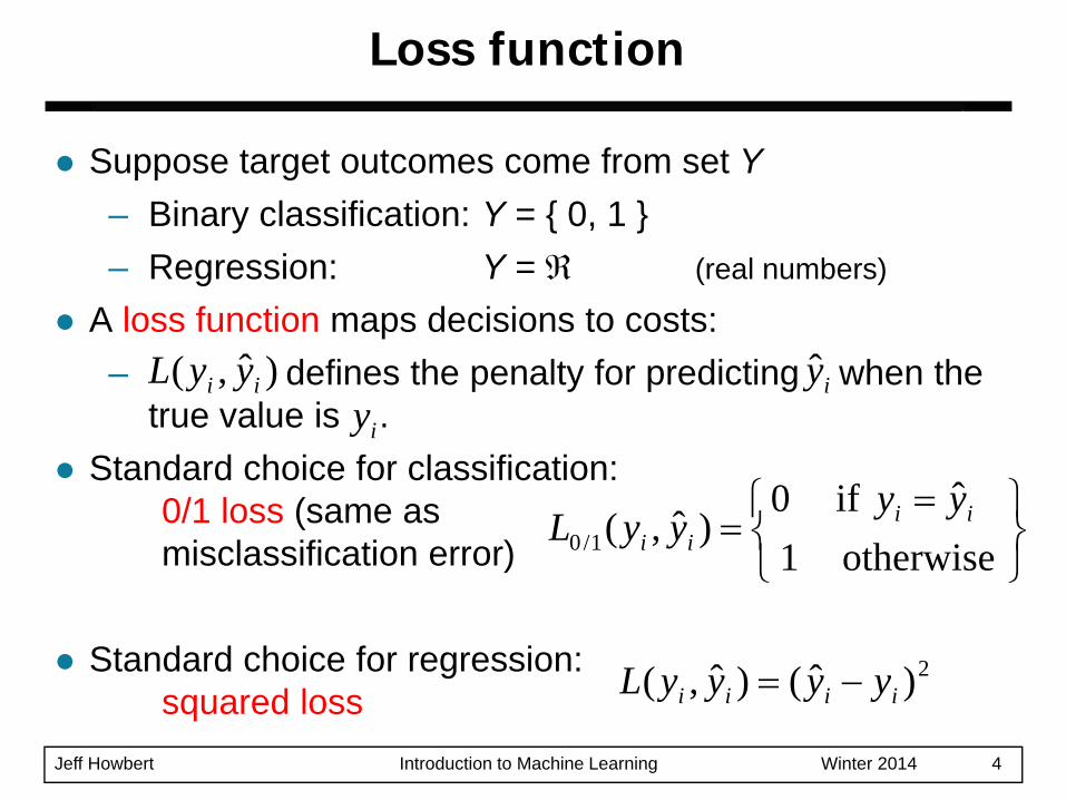
Suppose target outcomes come from set Y– Binary classification: Y = { 0, 1 }– Regression: Y = ℜ (real numbers)

A loss function maps decisions to costs:– defines the penalty for predicting when the

true value is .Standard choice for classification:

0/1 loss (same asmisclassification error)

Standard choice for regression:squared loss

Loss function

)ˆ,( ii yyL iyiy

⎭⎬⎫

⎩⎨⎧ =

=otherwise 1

ˆ if 0)ˆ,(1/0

iiii

yyyyL

2)ˆ()ˆ,( iiii yyyyL −=

Jeff Howbert Introduction to Machine Learning Winter 2014 5

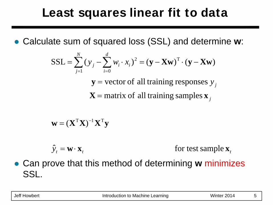
Calculate sum of squared loss (SSL) and determine w:

Can prove that this method of determining w minimizesSSL.

Least squares linear fit to data

ttt

j

j

N

j

d

iiij

y

y

xwy

xxw

yXXXw

xX

y

XwyXwy

samplefor test ˆ

)(

samples trainingall ofmatrix

responses trainingall ofvector

)()()(SSL

T1T

1

T2

0

⋅=

=

=

=

−⋅−=⋅−=

−

= =∑ ∑

Jeff Howbert Introduction to Machine Learning Winter 2014 6

Optimum of a function may be

– minimum or maximum

– global or local

Optimization

Jeff Howbert Introduction to Machine Learning Winter 2014 7

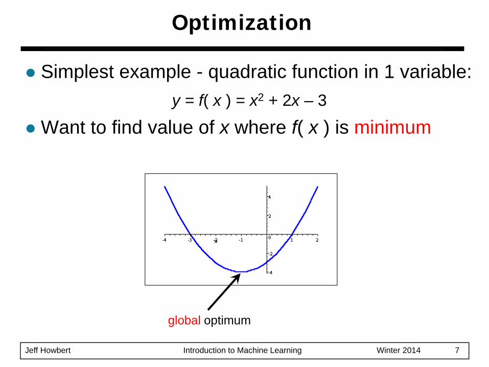
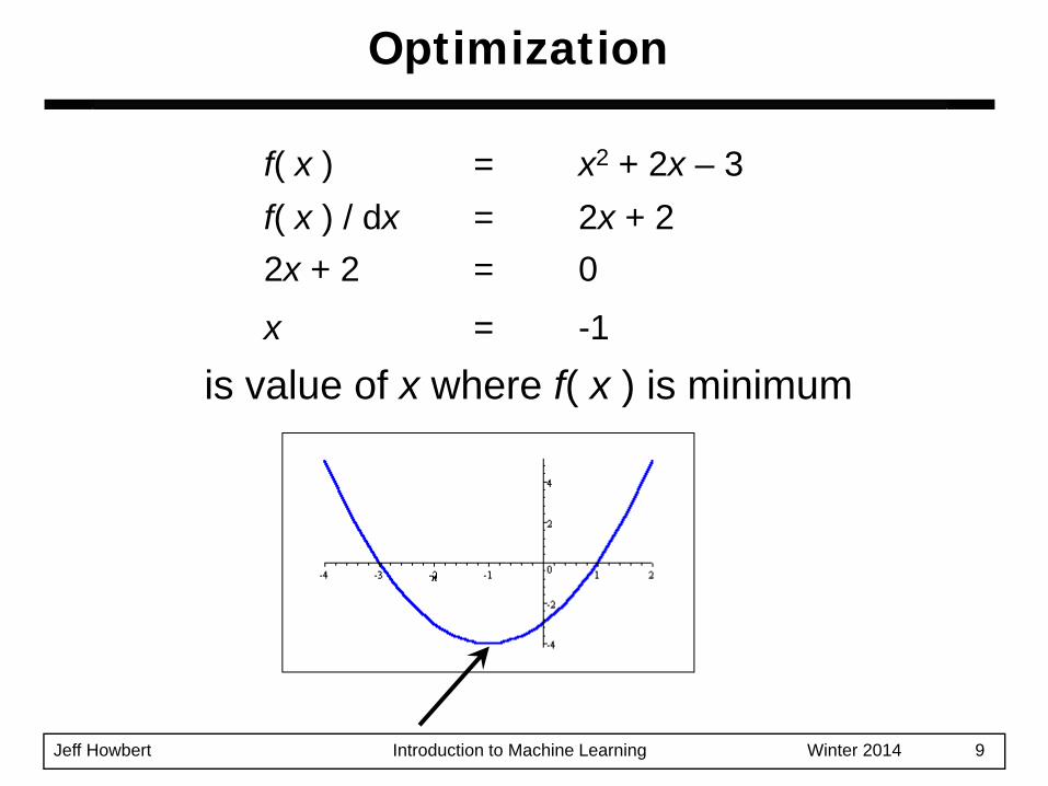
Simplest example - quadratic function in 1 variable:y = f( x ) = x2 + 2x – 3

Want to find value of x where f( x ) is minimum

Optimization

global optimum

Jeff Howbert Introduction to Machine Learning Winter 2014 8

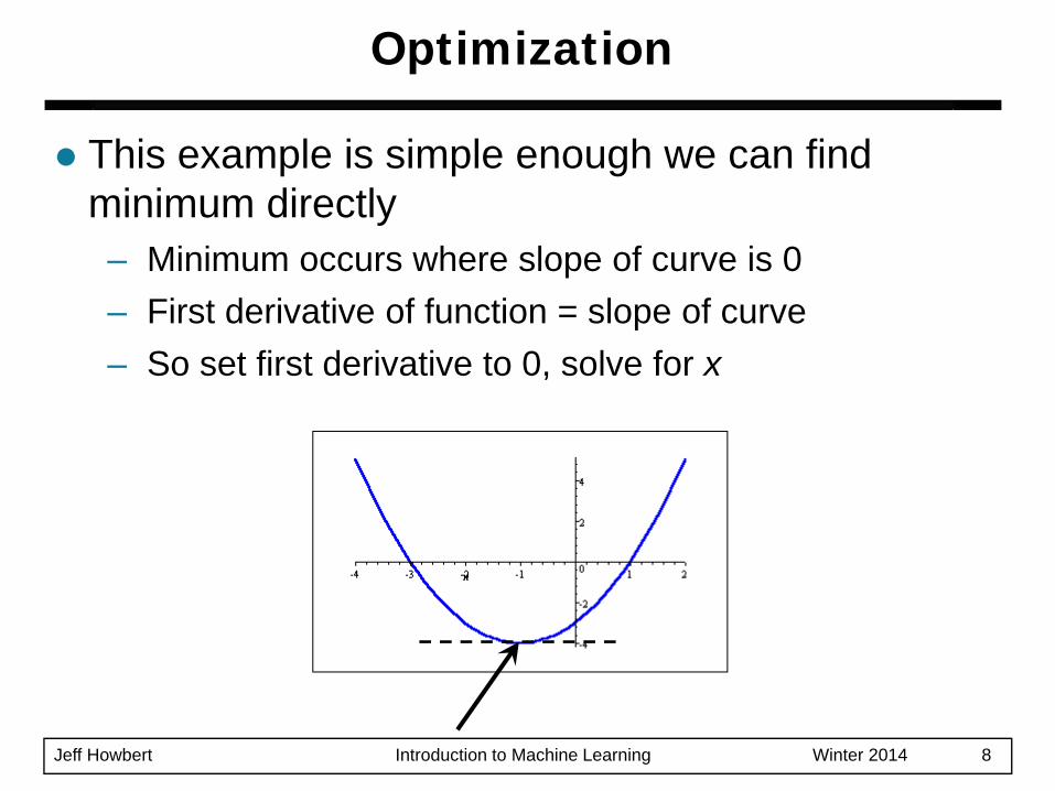
This example is simple enough we can find minimum directly– Minimum occurs where slope of curve is 0– First derivative of function = slope of curve– So set first derivative to 0, solve for x

Optimization

Jeff Howbert Introduction to Machine Learning Winter 2014 9

f( x ) = x2 + 2x – 3f( x ) / dx = 2x + 22x + 2 = 0

x = -1

is value of x where f( x ) is minimum

Optimization

Jeff Howbert Introduction to Machine Learning Winter 2014 10

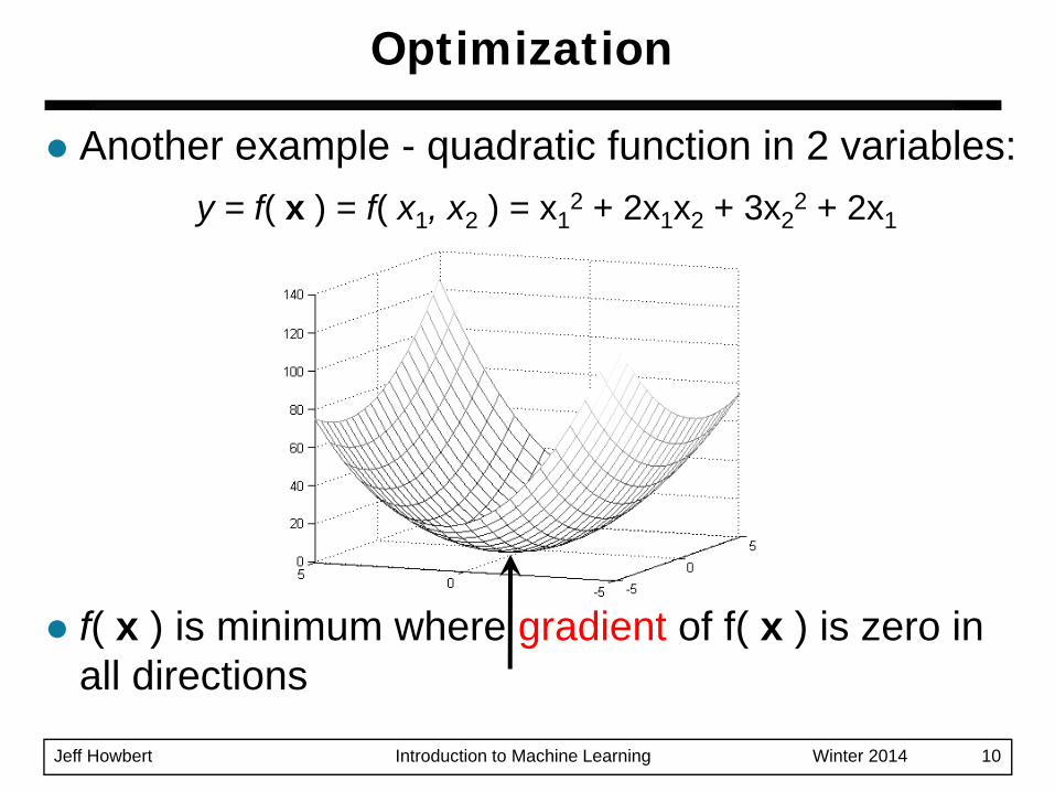
Another example - quadratic function in 2 variables:y = f( x ) = f( x1, x2 ) = x1

2 + 2x1x2 + 3x22 + 2x1

f( x ) is minimum where gradient of f( x ) is zero in all directions

Optimization

Jeff Howbert Introduction to Machine Learning Winter 2014 11

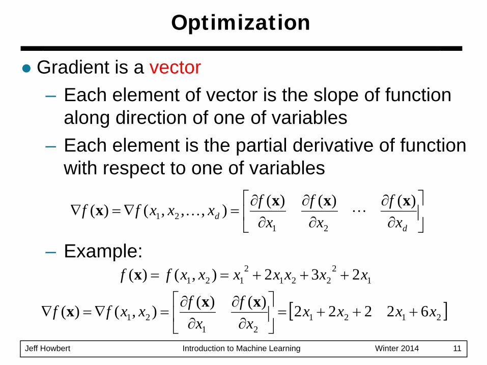
Gradient is a vector– Each element of vector is the slope of function

along direction of one of variables– Each element is the partial derivative of function

with respect to one of variables

– Example:

Optimization

⎥⎦

⎤⎢⎣

⎡∂∂

∂∂

∂∂

=∇=∇d

d xf

xf

xfxxxff )()()(),,,()(

2121

xxxx LK

[ ]212121

21

12

2212

121

62222)()(),()(

232),()(

xxxxx

fx

fxxff

xxxxxxxff

+++=⎥⎦

⎤⎢⎣

⎡∂∂

∂∂

=∇=∇

+++==

xxx

x

Jeff Howbert Introduction to Machine Learning Winter 2014 12

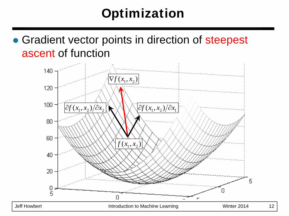
Gradient vector points in direction of steepest ascent of function

Optimization

121 ),( xxxf ∂∂

),( 21 xxf

),( 21 xxf∇

221 ),( xxxf ∂∂

Jeff Howbert Introduction to Machine Learning Winter 2014 13

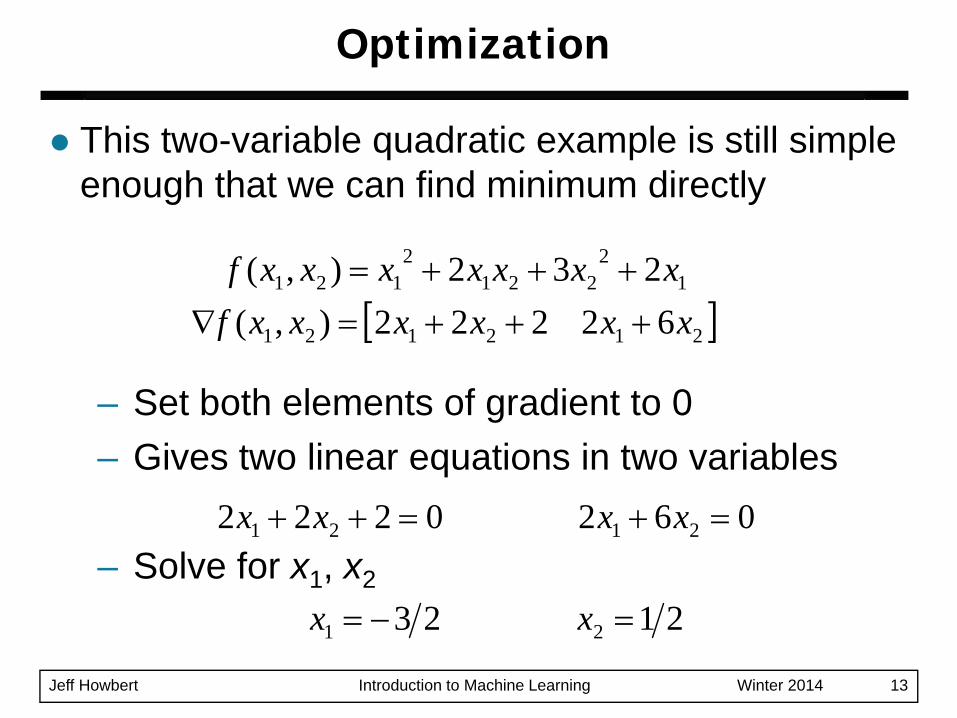
This two-variable quadratic example is still simple enough that we can find minimum directly

– Set both elements of gradient to 0– Gives two linear equations in two variables

– Solve for x1, x2

Optimization

[ ]212121

12

2212

121

62222),(232),(

xxxxxxfxxxxxxxf

+++=∇+++=

2123 21 =−= xx

0620222 2121 =+=++ xxxx

Jeff Howbert Introduction to Machine Learning Winter 2014 14

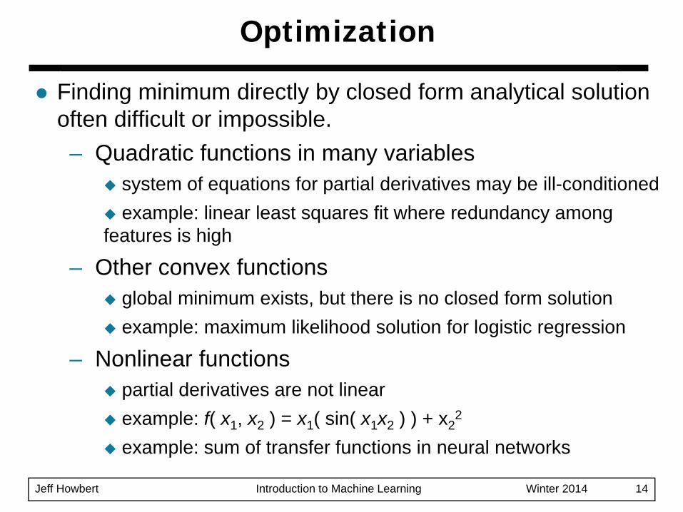
Finding minimum directly by closed form analytical solution often difficult or impossible.– Quadratic functions in many variables

system of equations for partial derivatives may be ill-conditionedexample: linear least squares fit where redundancy among

features is high

– Other convex functionsglobal minimum exists, but there is no closed form solutionexample: maximum likelihood solution for logistic regression

– Nonlinear functionspartial derivatives are not linearexample: f( x1, x2 ) = x1( sin( x1x2 ) ) + x2

2

example: sum of transfer functions in neural networks

Optimization

Jeff Howbert Introduction to Machine Learning Winter 2014 15

Many approximate methods for finding minima have been developed– Gradient descent– Newton method– Gauss-Newton– Levenberg-Marquardt– BFGS– Conjugate gradient– Etc.

Optimization

Jeff Howbert Introduction to Machine Learning Winter 2014 16

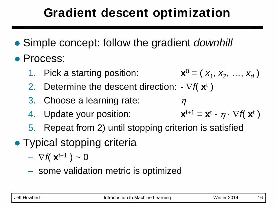
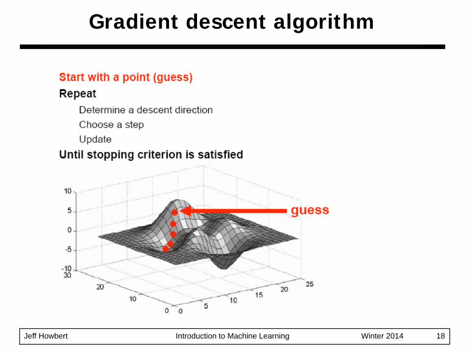
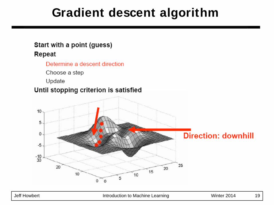
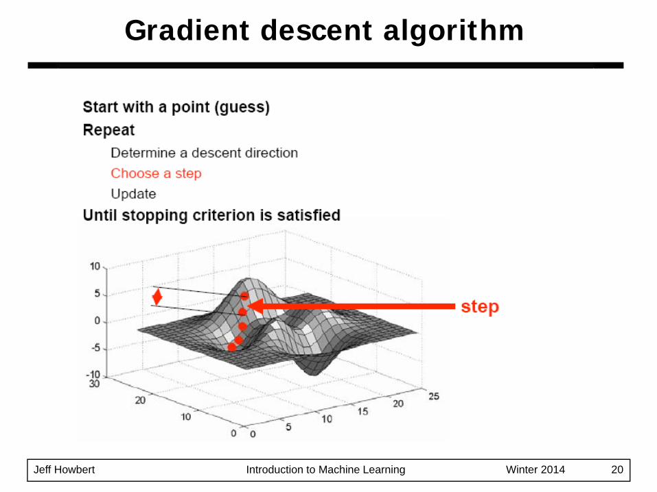
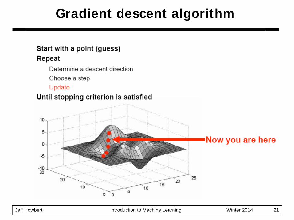
Simple concept: follow the gradient downhillProcess:1. Pick a starting position: x0 = ( x1, x2, …, xd )2. Determine the descent direction: - ∇f( xt )3. Choose a learning rate: η4. Update your position: xt+1 = xt - η ⋅ ∇f( xt )5. Repeat from 2) until stopping criterion is satisfied

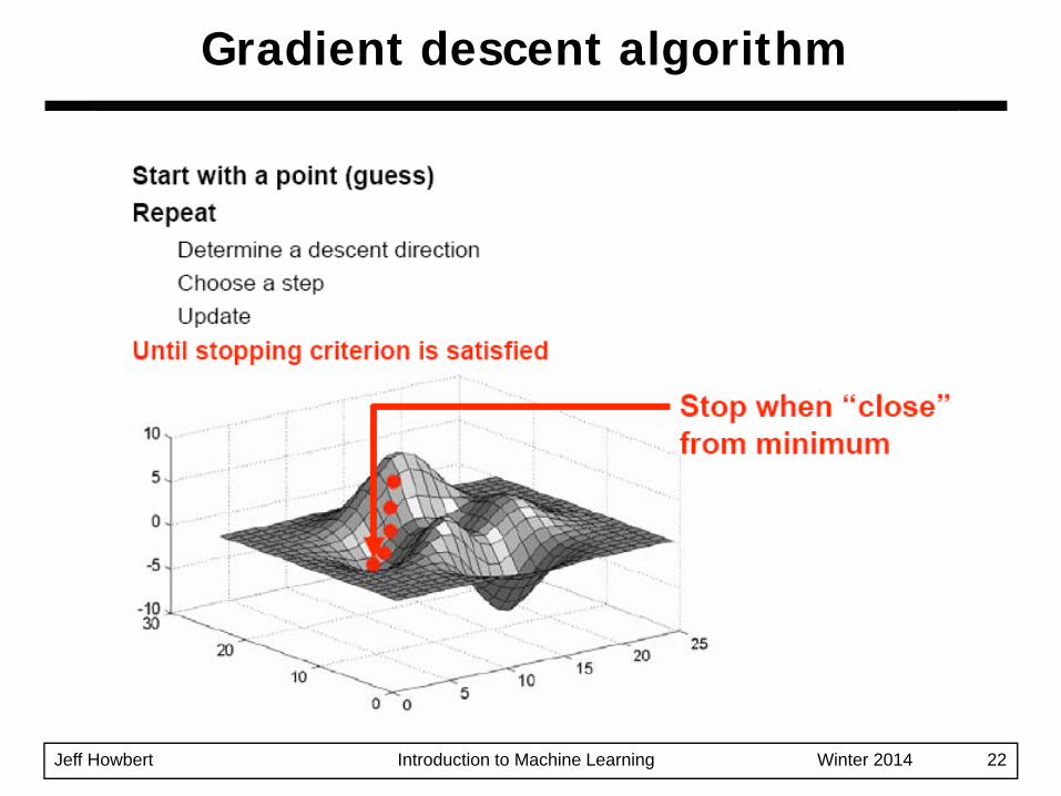
Typical stopping criteria– ∇f( xt+1 ) ~ 0– some validation metric is optimized

Gradient descent optimization

Jeff Howbert Introduction to Machine Learning Winter 2014 17

Slides thanks to Alexandre Bayen(CE 191, Univ. California, Berkeley, 2009)

http://bayen.eecs.berkeley.edu/bayen/?q=webfm_send/246

Gradient descent optimization

Jeff Howbert Introduction to Machine Learning Winter 2014 18

Gradient descent algorithm

Jeff Howbert Introduction to Machine Learning Winter 2014 19

Gradient descent algorithm

Jeff Howbert Introduction to Machine Learning Winter 2014 20

Gradient descent algorithm

Jeff Howbert Introduction to Machine Learning Winter 2014 21

Gradient descent algorithm

Jeff Howbert Introduction to Machine Learning Winter 2014 22

Gradient descent algorithm

Jeff Howbert Introduction to Machine Learning Winter 2014 23

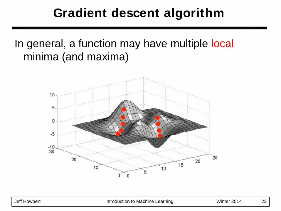
In general, a function may have multiple localminima (and maxima)

Gradient descent algorithm

Jeff Howbert Introduction to Machine Learning Winter 2014 24

Example in MATLAB

Find minimum of function in two variables:y = x1

2 + x1x2 + 3x22

http://www.youtube.com/watch?v=cY1YGQQbrpQ

Gradient descent optimization

Jeff Howbert Introduction to Machine Learning Winter 2014 25

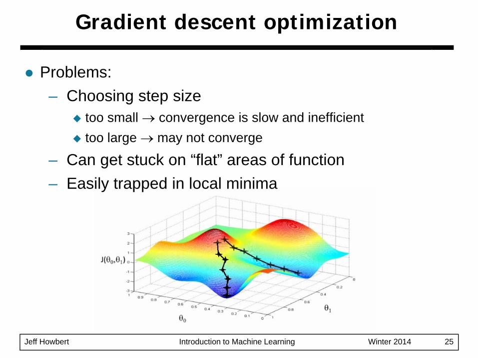
Problems:– Choosing step size

too small → convergence is slow and inefficienttoo large → may not converge

– Can get stuck on “flat” areas of function– Easily trapped in local minima

Gradient descent optimization

Jeff Howbert Introduction to Machine Learning Winter 2014 26

Stochastic (definition):1. involving a random variable2. involving chance or probability; probabilistic

Stochastic gradient descent

Jeff Howbert Introduction to Machine Learning Winter 2014 27

Application to training a machine learning model:1. Choose one sample from training set2. Calculate loss function for that single sample3. Calculate gradient from loss function4. Update model parameters a single step based on

gradient and learning rate5. Repeat from 1) until stopping criterion is satisfied

Typically entire training set is processed multiple times before stopping.Order in which samples are processed can be fixed or random.

Stochastic gradient descent

Jeff Howbert Introduction to Machine Learning Winter 2014 28

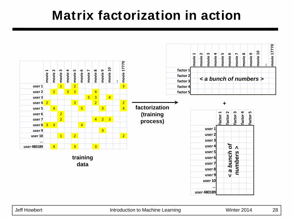
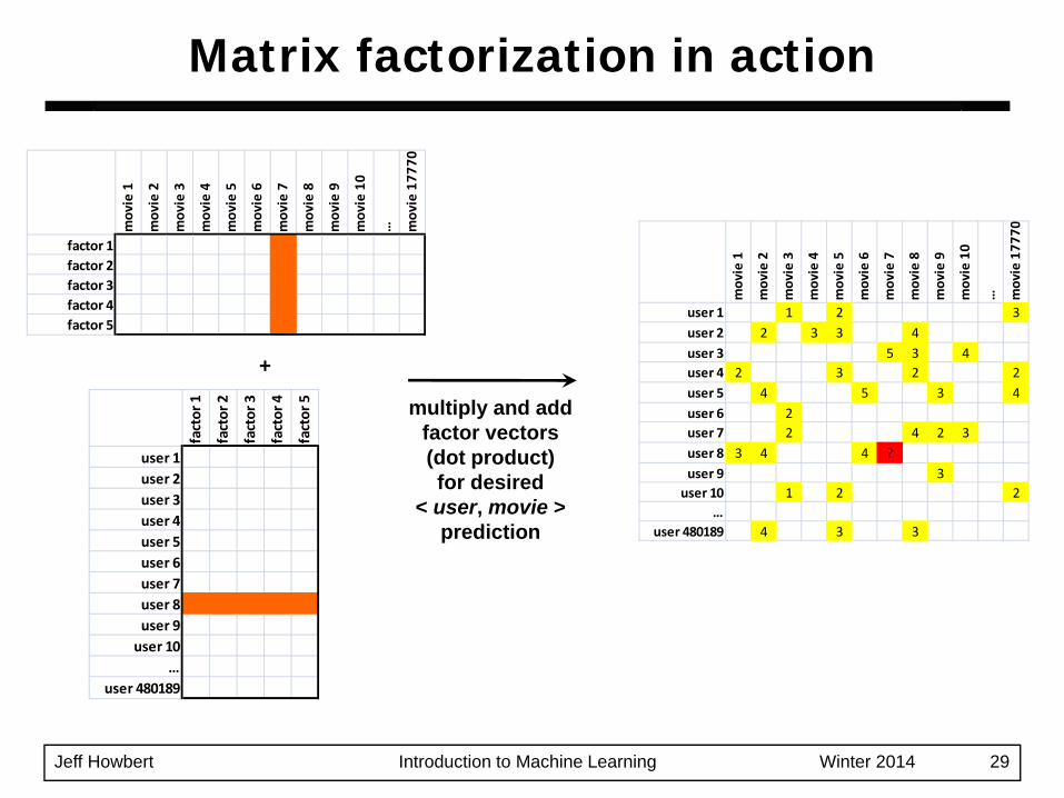
Matrix factorization in action

movie 1

movie 2

movie 3

movie 4

movie 5

movie 6

movie 7

movie 8

movie 9

movie 10

… movie 177

7 0

user 1 1 2 3user 2 2 3 3 4user 3 5 3 4user 4 2 3 2 2user 5 4 5 3 4user 6 2user 7 2 4 2 3user 8 3 4 4user 9 3user 10 1 2 2

…user 480189 4 3 3

movie 1

movie 2

movie 3

movie 4

movie 5

movie 6

movie 7

movie 8

movie 9

movie 10

… movie 177

70

factor 1factor 2factor 3factor 4factor 5

< a bunch of numbers >

factor 1

factor 2

factor 3

factor 4

factor 5

user 1user 2user 3user 4user 5user 6user 7user 8user 9user 10

…user 480189

< a

bunc

h of

num

bers

>

factorization(trainingprocess)

+

trainingdata

Jeff Howbert Introduction to Machine Learning Winter 2014 29movie 1

movie 2

movie 3

movie 4

movie 5

movie 6

movie 7

movie 8

movie 9

movie 10

… movie 177

7 0

user 1 1 2 3user 2 2 3 3 4user 3 5 3 4user 4 2 3 2 2user 5 4 5 3 4user 6 2user 7 2 4 2 3user 8 3 4 4 ?user 9 3user 10 1 2 2

…user 480189 4 3 3

movie 1

movie 2

movie 3

movie 4

movie 5

movie 6

movie 7

movie 8

movie 9

movie 10

… movie 177

70

factor 1factor 2factor 3factor 4factor 5

factor 1

factor 2

factor 3

factor 4

factor 5

user 1user 2user 3user 4user 5user 6user 7user 8user 9user 10

…user 480189

multiply and addfactor vectors(dot product)for desired

< user, movie >prediction

+

Matrix factorization in action

Jeff Howbert Introduction to Machine Learning Winter 2014 30

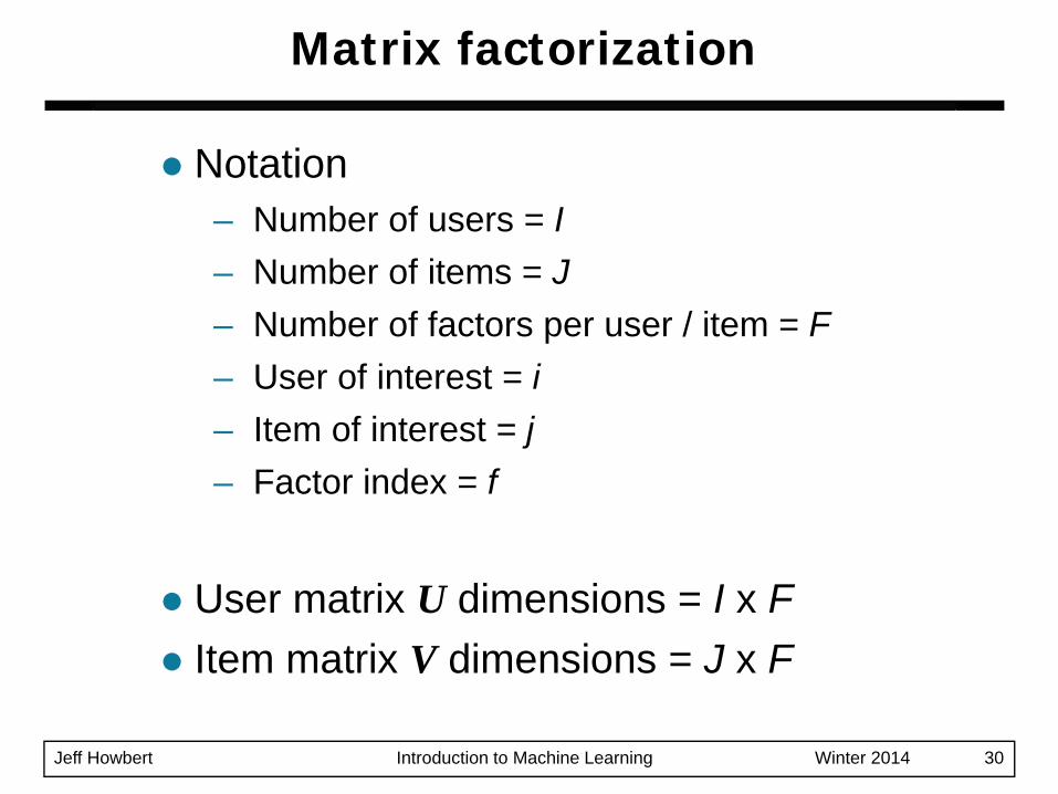
Notation– Number of users = I– Number of items = J– Number of factors per user / item = F– User of interest = i– Item of interest = j– Factor index = f

User matrix U dimensions = I x FItem matrix V dimensions = J x F

Matrix factorization

Jeff Howbert Introduction to Machine Learning Winter 2014 31

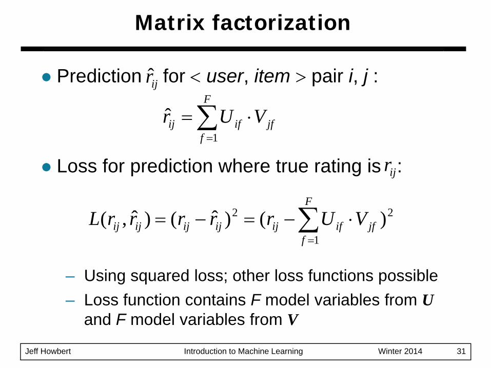
Prediction for < user, item > pair i, j :

Loss for prediction where true rating is :

– Using squared loss; other loss functions possible– Loss function contains F model variables from U

and F model variables from V

Matrix factorization

∑=

⋅=F

fjfifij VUr

1

ˆ

ijr

ijr

∑=

⋅−=−=F

fjfifijijijijij VUrrrrrL

1

22 )()ˆ()ˆ,(

Jeff Howbert Introduction to Machine Learning Winter 2014 32

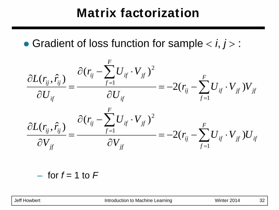
Gradient of loss function for sample < i, j > :

– for f = 1 to F

Matrix factorization

∑∑

∑∑

=

=

=

=

⋅−−=∂

⋅−∂=

∂

∂

⋅−−=∂

⋅−∂=

∂

∂

F

fifjfifij

jf

F

fjfifij

jf

ijij

F

fjfjfifij

if

F

fjfifij

if

ijij

UVUrV

VUr

VrrL

VVUrU

VUr

UrrL

1

1

2

1

1

2

)(2)(

)ˆ,(

)(2)(

)ˆ,(

Jeff Howbert Introduction to Machine Learning Winter 2014 33

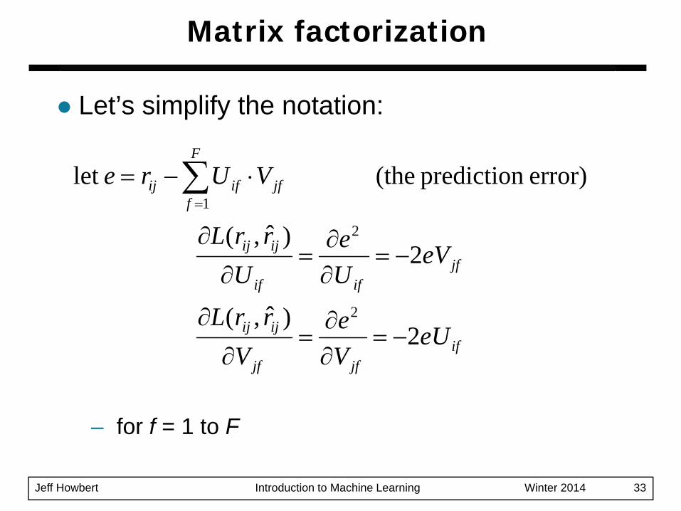
Let’s simplify the notation:

– for f = 1 to F

Matrix factorization

ifjfjf

ijij

jfifif

ijij

F

fjfifij

eUVe

VrrL

eVUe

UrrL

VUre

2)ˆ,(

2)ˆ,(

error) prediction (the let

2

2

1

−=∂∂

=∂

∂

−=∂∂

=∂

∂

⋅−= ∑=

Jeff Howbert Introduction to Machine Learning Winter 2014 34

Matrix factorization

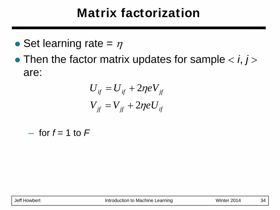
Set learning rate = ηThen the factor matrix updates for sample < i, j >are:

– for f = 1 to F

ifjfjf

jfifif

eUVV

eVUU

η

η

2

2

+=

+=

Jeff Howbert Introduction to Machine Learning Winter 2014 35

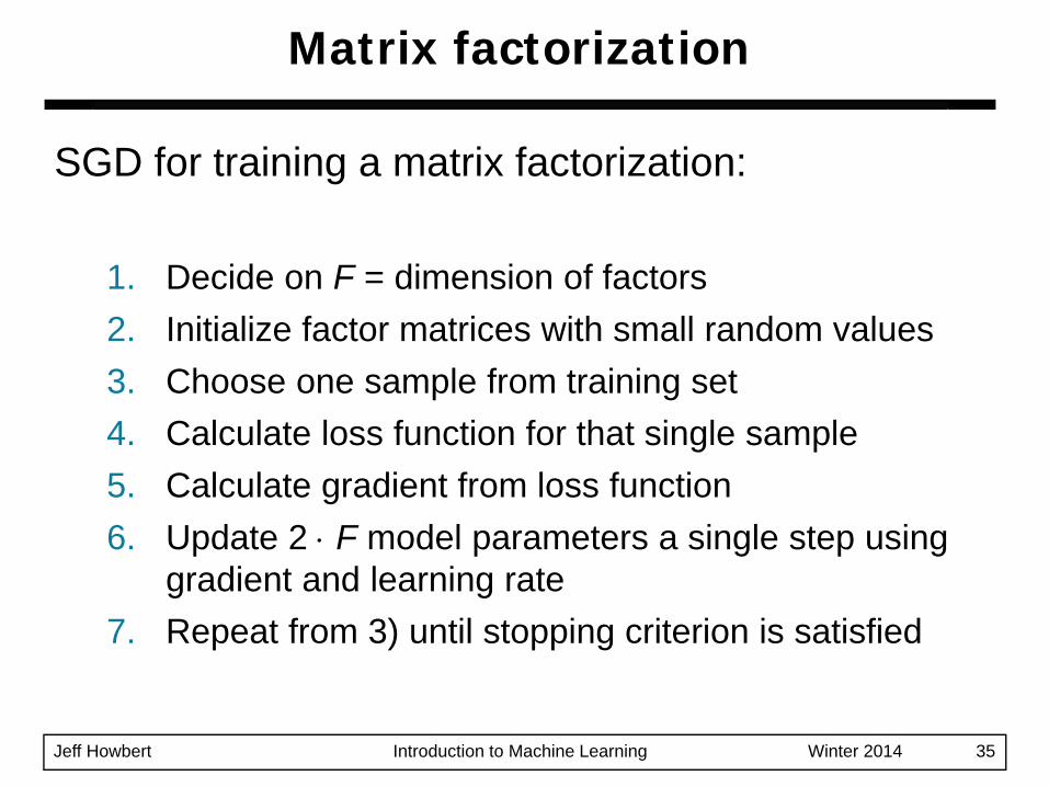
SGD for training a matrix factorization:

1. Decide on F = dimension of factors2. Initialize factor matrices with small random values3. Choose one sample from training set4. Calculate loss function for that single sample5. Calculate gradient from loss function6. Update 2 ⋅ F model parameters a single step using

gradient and learning rate7. Repeat from 3) until stopping criterion is satisfied

Matrix factorization

Jeff Howbert Introduction to Machine Learning Winter 2014 36

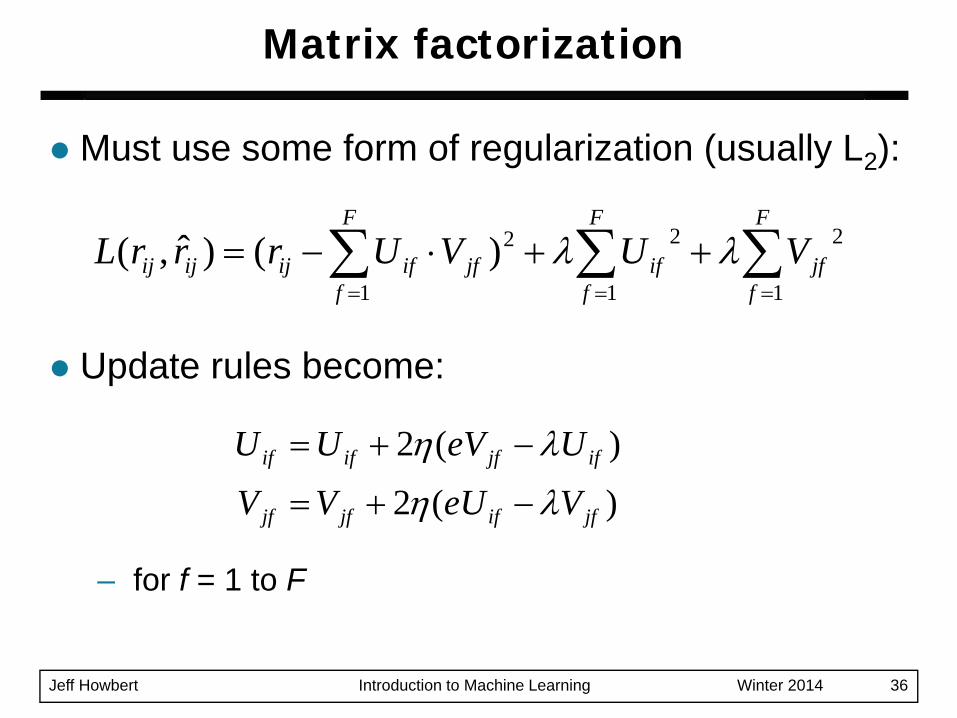
Must use some form of regularization (usually L2):

Update rules become:

– for f = 1 to F

Matrix factorization

∑ ∑∑= ==

++⋅−=F

f

F

fjf

F

fifjfifijijij VUVUrrrL

1 1

2

1

22)()ˆ,( λλ

)(2

)(2

jfifjfjf

ifjfifif

VeUVV

UeVUU

λη

λη

−+=

−+=

Jeff Howbert Introduction to Machine Learning Winter 2014 37

Random thoughts …– Samples can be processed in small batches

instead of one at a time → batch gradient descent

– We’ll see stochastic / batch gradient descent again when we learn about neural networks (as back-propagation)

Stochastic gradient descent