collection of terms, symbols, equations, and explanations of … · glossary page 2 of...

$: Collection of terms, symbols, equations, and explanations of … · Glossary Page 2 of 24...\PK-glossary_PK_working_group_2004.pdf Collection of terms, symbols, equations, and explanations$
Glossary Page 1 of 24

...\PK-glossary_PK_working_group_2004.pdf

Collection of terms, symbols, equations, and

explanations of common pharmacokinetic and pharmacodynamic parameters and some

statistical functions

Version: 16 Februar 2004 Authors: AGAH working group PHARMACOKINETICS

Glossary Page 2 of 24


Collection of terms, symbols, equations, and explanations of common pharmacokinetic and pharmacodynamic parameters and some

statistical functions TABLE OF CONTENTS Page

TABLE OF CONTENTS .................................................................................................................2

1 Pharmacokinetic Parameters from noncompartmental analysis (NCA) ...............................3 1.1 Parameters obtained from concentrations in plasma or serum...........................................3

1.1.1 Parameters after single dosing..................................................................................3 1.1.2 Parameters after multiple dosing (at steady state)....................................................6

1.2 Parameters obtained from urine ..........................................................................................7

2 Pharmacokinetic parameters obtained from compartmental modeling................................8 2.1 Calculation of concentration-time curves.............................................................................9 2.2 Pharmacokinetic Equations - Collection of Equations for Compartmental Analysis .........10

3 Pharmacodynamic GLOSSARY................................................................................................20 3.1 Definitions ..........................................................................................................................20 3.2 Equations: PK/PD Models..................................................................................................21

4 Statistical parameters................................................................................................................22 4.1 Definitions ..........................................................................................................................22 4.2 Characterisation of log-normally distributed data ..............................................................23

AGAH Working group PK/PD modelling Page 3 of 24


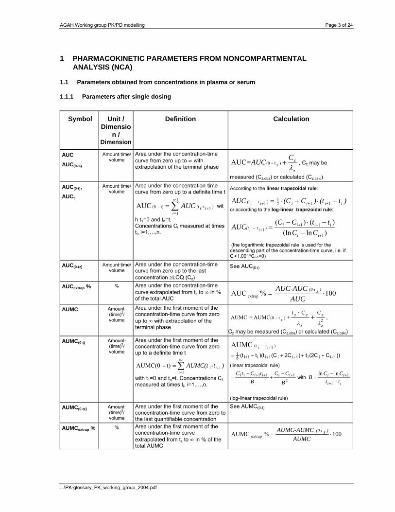
1 PHARMACOKINETIC PARAMETERS FROM NONCOMPARTMENTAL ANALYSIS (NCA)

1.1 Parameters obtained from concentrations in plasma or serum

1.1.1 Parameters after single dosing

Symbol Unit / Dimensio

n / Dimension

Definition Calculation

AUC

AUC(0-∞)

Amount·time/ volume

Area under the concentration-time curve from zero up to ∞ with extrapolation of the terminal phase

z

z)zt-(0AUC

λC=AUC + , Cz may be

measured (Cz,obs) or calculated (Cz,calc) AUC(0-t), AUCt


Area under the concentration-time curve from zero up to a definite time t

∑ +=1

11t)-(0 AUC

n-

i=)i-ti(t AUC wit

h t1=0 and tn=t, Concentrations Ci measured at times ti, i=1,…,n.

According to the linear trapezoidal rule:

) t(t)C(CAUC ii+i+iiti(t −⋅+⋅=+− 1121)1

or according to the log-linear trapezoidal rule:

)ln(ln)()(

1

11)1

+

+++−

−−⋅−

=ii

iiiiiti(t

CCttCC

AUC

(the logarithmic trapezoidal rule is used for the descending part of the concentration-time curve, i.e. if Ci>1.001*Ci+1>0)

AUC(0-tz) Amount·time/ volume

Area under the concentration-time curve from zero up to the last concentration ≥LOQ (Cz)

See AUC(0-t)

AUCextrap % % Area under the concentration-time curve extrapolated from tz to ∞ in % of the total AUC

100%AUC extrap ⋅=AUC

AUC-AUC )z(0-t

AUMC Amount· (time)2/ volume

Area under the first moment of the concentration-time curve from zero up to ∞ with extrapolation of the terminal phase

2z

z

z

zz)zt-(0

CCt +AUMC =AUMC

λλ+

⋅,

Cz may be measured (Cz,obs) or calculated (Cz,calc)

AUMC(0-t) Amount· (time)2/ volume

Area under the first moment of the concentration-time curve from zero up to a definite time t

∑ +=1

11 t)-AUMC(0

n-

i=ii ) -tAUMC(t

with t1=0 and tn=t. Concentrations Ci measured at times ti, i=1,…,n.

)1i(tAUMC +− it

))C(2Ct)2C(C)(tt(t 1iii1ii1ii1+i +++ +++−= 61

(linear trapezoidal rule)

2111

B

CCB

tCtC iiiiii +++ −+

−= with

ii

iittCC

B−

−=

+

+

1

1lnln

(log-linear trapezoidal rule)

AUMC(0-tz) Amount· (time)2/ volume

Area under the first moment of the concentration-time curve from zero to the last quantifiable concentration

See AUMC(0-t)

AUMCextrap % % Area under the first moment of the concentration-time curve extrapolated from tz to ∞ in % of the total AUMC

100%AUMC extrap ⋅=AUMC

AUMC-AUMC )z(0-t



Symbol Unit / Dimension


Cp or C Amount/ volume Plasma concentration Cs or C Amount/ volume Serum concentration Cu Amount/ volume Unbound plasma concentration CL Volume/ time or

volume/ time/ kg Total plasma, serum or blood clearance of drug after intravenous administration

CL =D

AUCiv

CL / f Volume/ time or volume/ time/ kg

Apparent total plasma or serum clearance of drug after oral administration

CL / f =DAUC

po

CLint Volume/ time or volume/ time/ kg

Intrinsic clearance – maximum elimination capacity of the liver

CLH,b Volume/ time or volume/ time/ kg

Hepatic blood clearance, product of hepatic blood flow and extraction ratio

CLH = QH·EH

CLCR Volume/ time or volume/ time/ kg

Creatinine clearance Measured or Cockcroft & Gault formula

CLm Volume/ time Metabolic clearance Cz, calc Amount/ volume Predicted last plasma or serum

concentration Calculated from a log-linear regression through the terminal part of the curve

Cz or Cz, obs Amount/ volume Last analytically quantifiable plasma or serum concentration above LOQ

directly taken from analytical data

Cmax Amount/ volume Observed maximum plasma or serum concentration after administration


D Amount Dose administered

f - Fraction of the administered dose systemically available f =

AUC DAUC D

po iv

iv po

⋅

⋅

F % Absolute bioavailability, systemic availability in %

F = f 100⋅

frel - Fraction of the administered dose in comparison to a standard (not iv) D AUC

D AUC fSTD

STDrel ⋅

⋅= STD = Standard

Frel % Relative bioavailability in % 100f = F relrel ⋅

fa - Fraction of the extravascularly administered dose actually absorbed

For orally administered drugs: f = fa*(1-EH)

fm - Fraction of the bioavailable dose which is metabolized

fu - Fraction of unbound (not protein-bound or free) drug in plasma or serum

fu = Cu /C

HVD Time Half-value duration (time interval during which concentrations exceed 50% of Cmax)

λz (Time)-1 Terminal rate constant (slowest rate constant of the disposition)

negative of the slope of a ln-linear regression of the unweighted data considering the last concentration-time points ≥ LOQ

ke or kel (Time)-1 Elimination rate constant from the central compartment

calculated from parameters of the multiexponential fit

LOQ Amount/ volume Lower limit of quantification





MAT Time Mean absorption time MAT = MRT - MRTev iv (ev = extravasal, e.g. im, sc, po)

MDT Time Mean dissolution time

MRT Time Mean residence time (of the unchanged drug in the systemic circulation)

MRT = AUMCAUC

MR - Metabolic ratio of parent drug AUC and metabolite AUC MR =

AUCAUC

parent

metabolite

t1/2 Time Terminal half-life 1/ 2t =

ln 2zλ

tlag Time

Lag-time (time delay between drug administration and first observed concentration above LOQ in plasma)


tz Time Time p.a. of last analytically quantifiable concentration


tmax Time Time to reach Cmax directly taken from analytical data

Vss Volume

or volume/kg

Apparent volume of distribution at equilibrium determined after intravenous administration

2(AUC)AUMCD = MRTCL = Vss⋅

⋅

Vz Volume

or volume/kg

Volume of distribution during terminal phase after intravenous administration

zAUC λ⋅= ivD

V z

Vss / f Volume

or volume/kg

Apparent volume of distribution at equilibrium after oral administration 2(AUC)

AUMCD = MRTCL = /fVss⋅

⋅

Vz / f Volume

or volume/kg

Apparent volume of distribution during terminal phase after oral / extravascular administration

zλAUCf

⋅= poD

/Vz po instead of iv !



1.1.2 Parameters after multiple dosing (at steady state)



Aave Amount Average amount in the body at steady state

τλz ⋅⋅ M

aveDf = A

AUCτ,ss

AUCss


Area under the concentration-time curve during a dosing interval at steady state

by trapezoidal rule

AUCF% % Percent fluctuation of the concentrations determined from areas under the curve AUC

AUC+AUC100 =AUCF%

)C (below)C (above aveave⋅

Cav,ss Amount /volume

Average plasma or serum concentration at steady state τ

τ ss,AUC=C ssav,

Cmax,ss Amount /volume

Maximum observed plasma or serum concentration during a dosing interval at steady state


Cmin,ss Amount /volume

Minimum observed plasma or serum concentration during a dosing interval at steady state


Ctrough Amount /volume

Measured concentration at the end of a dosing interval at steady state (takendirectly before next administration)


DM Amount Maintenance dose design parameter

LF - Linearity factor of pharmacokinetics after repeated administration

sd

ss,=

AUCAUC

LF τ sd = single dose

PTF % % Peak trough fluctuation over one dosing interval at steady state

avss,

minss,maxss,

CC-C

100 % PTF ⋅=

RA (AUC) Accumulation ratio calculated from AUCτ,ss at steady state and AUCτ after single dosing

R A (AUC) =sd

AUCAUC

ssτ

τ

,

,

RA (Cmax) Accumulation ratio calculated from Cmax,ss at steady state and Cmax after single dosing

RA (Cmax) =CC

ss

sd

max,

max, sd = single dose

RA (Cmin) Accumulation ratio calculated from Cmin,ss at steady state and from concentration at t=τ after single dose sd

ssC

C

,

min,= A (Cmin) Rτ

sd = single dose

Rtheor Theoretical accumulation ratio τλε ze−−

=1

12-11

= theor -R , 2/1t

τε =

TCave Time Time period during which plasma concentrations are above Cav,ss

derived from analytical data by linear interpolation

tmax,ss Time Time to reach the observed maximum (peak) concentration at steady state


τ Time Dosing interval directly taken from study design



1.2 Parameters obtained from urine



Ae(t1-t2) Amount Amount of unchanged drug excreted into urine within time span from t1 to t2.

Cur * Vur

Ae(0-�) Amount Cumulative amount (of unchanged drug) excreted into urine up to infinity after single dosing

(can commonly not be determined)

Aeτ,ss Aess

Amount Amount (of unchanged drug) excreted into the urine during a dosing interval (τ) at steady state

Cur Amount/ volume

Drug concentration in urine

CLR Volume/ time or volume/

time/ amount

Renal clearance

)0()0()0(ττ−−

≈∞−

=AUC

AeAUC

AeCLR

after multiple dose ss

R AUCAeCL

,

)0(

τ

τ−=

fe - Fraction of intravenous administered

drug that is excreted unchanged in urine iv

ee D

A = f

fe/f - Fraction of orally administered drug excreted into urine ef

AD

epo

/ f =

Fe % Total urinary recovery after intravenous administration = fraction of drug excreted into urine in %

Fe = fe ⋅ 100

tmid Time Mid time point of a collection interval

Vur Volume Volume of urine excreted directly taken from measured lab data



2 PHARMACOKINETIC PARAMETERS OBTAINED FROM COMPARTMENTAL MODELING

Symbol Unit / Dimensions


A,B,C or Ci, i=1,...,n

Amount/ volume Coefficients of the polyexponential equation

by multiexponential fitting

α, β, γ (Time)-1 Exponents of the polyexponential equation (slope factor)


λI (Time)-1 Exponent of the ith (descending) exponential term of a polyexponential equation


AUC Amount·time/ volume

Area under the curve (model)

∑

∑

=

=

⎥⎦

⎤⎢⎣

⎡⎟⎟⎠

⎞⎜⎜⎝

⎛−

λ⋅

λ−⋅=

⎥⎦

⎤⎢⎣

⎡λ

=

n

1i aiia

ai

n

1i i

i

k11

kkCAUC

:larextravascu

CAUC:iv

Note: Ci is the linear coefficient of the polyexponential equation

AUMC Amount·(time)2/ volume

Area under the first moment curve

∑

∑

=

=

⎥⎦

⎤⎢⎣

⎡⎟⎟⎠

⎞⎜⎜⎝

⎛−

λ⋅

λ−⋅=

⎥⎦

⎤⎢⎣

⎡

λ=

n

1i2a

2iia

ai

n

1i2

i

i

k11

kkCAUMC

:larextravascu

CAUMC:iv


C(0) Amount/ volume Initial or back-extrapolated drug concentration following rapid intravenous injection

∑=n

1=iiC)0(C


C(t) Amount/ volume Drug concentration at time point t See 2.2 CL Volume/ time Clearance

AUCDosefCL ⋅

= iv: f=1

fi - Fractional area, area under the various phases of disposition (λi) in the plasma concentration-time curve after iv dosing

1fwithAUC

C

fn

1ii

i

i

i =λ

= ∑=

i Number of compartments in a multi-compartmental model

k0 (Time)-1 Zero order rate constant Design parameter or determined by multiexponential fitting

ke or kel (Time)-1 Elimination rate constant from the central compartment

calculated from parameters of the multiexponential fit

ka or kabs (Time)-1 Absorption rate constant by multiexponential fitting

kij (Time)-1 Transfer rate between compartment i and j in a multi-compartmental model


Km Amount/ volume Michaelis –Menten constant by nonlinear fitting



Symbol Unit / Dimensions


MRT Time Mean residence time iv:

AUCAUMCMRT =

extravascular: )1(a

lag kt

AUCAUMCMRT +−=

Qi Amount/Time Intercompartmental clearance between central compartment and compartment i

k0 Amount/Time Zero order infusion rate design parameter

t 1/2, iλ Time Half-life associated with the ith

exponent of a polyexponential equation t ln21/2, iλ λ

=i

τ Time Infusion duration design parameter

t Time Time after drug administration

Vc Volume or Volume /amount

Apparent volume of the central or plasma or serum compartment

∑=

⋅= n

1ii

c

C

DosefV

iv: f=1

Vmax Amount/Time Maximum metabolic rate



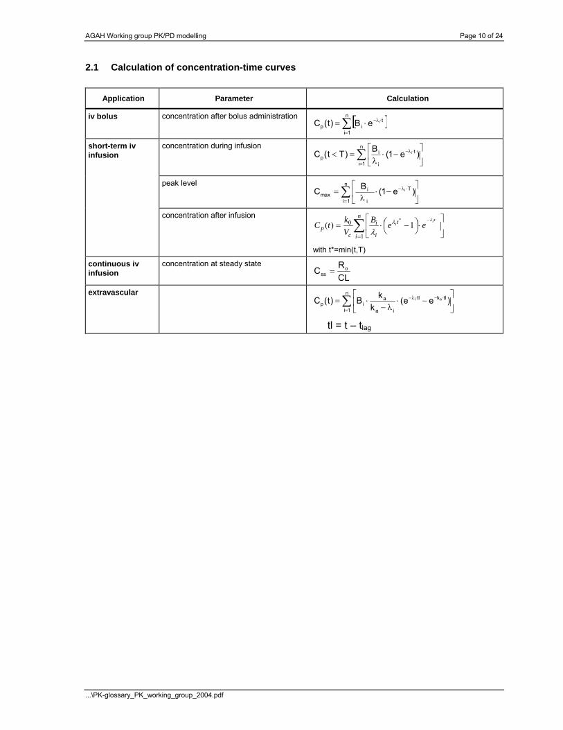
2.1 Calculation of concentration-time curves

Application Parameter Calculation

iv bolus concentration after bolus administration

[ ]∑=

⋅λ−⋅=n

1i

tip

ieB)t(C

concentration during infusion ∑=

⋅λ−⎥⎦

⎤⎢⎣

⎡−⋅

λ=<

n

1i

t

i

ip )e1(B)Tt(C i

peak level ∑=

⋅λ−⎥⎦

⎤⎢⎣

⎡−⋅

λ=

n

1i

T

i

imax )e1(BC i

short-term iv infusion

concentration after infusion ∑=

⎥⎦

⎤⎢⎣

⎡⋅⎟⎠⎞⎜

⎝⎛ −⋅=

−n

i

t

i

i

cp

tii eeB

VktC

1

0 1)(* λλ

λ

with t*=min(t,T)

continuous iv infusion

concentration at steady state

CLRC o

ss =

extravascular ∑=

⋅−⋅λ−⎥⎦

⎤⎢⎣

⎡−⋅

λ−⋅=

n

1i

tlktl

ia

aip )ee(

kkB)t(C ai

tl = t – tlag



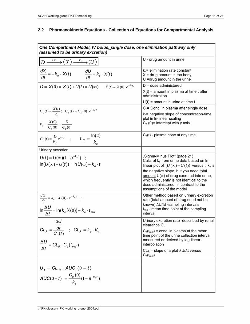
2.2 Pharmacokinetic Equations - Collection of Equations for Compartmental Analysis One Compartment Model, IV bolus, single dose, one elimination pathway only (assumed to be urinary excretion)

D X Ui v ke. .⎯ →⎯ ⎯ →⎯ U - drug amount in urine

)(tXkdtdX

e ⋅−= )(tXkdtdU

e ⋅= ke= elimination rate constant X = drug amount in the body U =drug amount in the urine

)()()()( ∞=+== UtUtXXD 0 etkeXtX ⋅−⋅= )0()( D = dose administered X(t) = amount in plasma at time t after administration U(t) = amount in urine at time t

cp V

tXtC )()( = ; tkpp

eeCtC ⋅−⋅= )0()(

)0()0()0(

ppc C

DCXV ==

Cp= Conc. in plasma after single dose ke= negative slope of concentration-time plot in ln-linear scaling Cp (0)= intercept with y axis

tk

dp

eeVDtC ⋅−=)( ;

ekt )ln(

/2

21 = Cp(t) - plasma conc at any time

Urinary excretion

))(()( tkeeUtU −−∞= 1 ;

tkUtUU e ⋅−∞=−∞ )(ln))()(ln(

„Sigma-Minus Plot“ (page 21) Calc. of ke from urine data based on ln-linear plot of ))()(( tUU −∞ versus t, ke is the negative slope, but you need total amount U(∞) of drug excreted into urine, which frequently is not identical to the dose administered, in contrast to the assumptions of the model

tke

eeXkdt

dU ⋅−⋅⋅= )0( ;

midee tkXktU

⋅−= ))(ln(∆∆ln 0

Other method based on urinary excretion rate (total amount of drug need not be known) ∆U/∆t -sampling intervals tmid - mean time point of the sampling interval

)(p tCdtdU

CLR = ; ceR VkCL ⋅=

)(∆∆

p midR tCCLtU

⋅=

Urinary excretion rate -described by renal clearance CLR Cp(tmid) = conc. in plasma at the mean time point of the urine collection interval, measured or derived by log-linear interpolation CLR = slope of a plot ∆U/∆t versus Cp(tmid)

)( tAUCCLU Rt −⋅= 0

)()(

)( p tk

e

etek

CtAUC −−=− 1

00



One Compartment Model, IV Inj. and Parallel Elimination Pathways (renal, biliary, metabolic), single dose

metbilrene kkkk ++= kren = rate constant of renal elimination kbil = rate constant of biliary elimination kmet = rate constant of metabolic elimination

)(tXkdtdX

e−= ; )(tXkdtdU

ren= ; )(tXkdtdB

bil= ;

)(tXkdt

dMmet=

X = amount in plasma U = amount in urine B = amount in bile M = amount of metabolites in plasma

)()()()()()()()( ∞+∞+∞=+++== MBUtMtBtUtXXD 0

tkpp

eeCtC −⋅= )()( 0 Plasma concentration

)()( tk

e

ren eeDkk

tU −−⋅⋅= 1 Drug amount in urine

Dkk

Ue

ren=∞)( ; e

ren

kk

DU

=∞)(

;

tkUtUU e ⋅−∞=−∞ )(ln))()(ln(

crenR VkCL ⋅= ⋅ ; )( b

RuR f

CLCL−

=1

Up to infinite time (t = ∝) ke - slope can calc.from the Sigma Minus Plot (U(∞)-U(t) vs t fb – fraction of bound drug

)()( tk

e

bil eeDkk

tB −−⋅⋅= 1 ; cbilbil VkCL ⋅= ⋅ Biliary excretion can be calc. In analogous fashion assuming no reabsorption

)()( tk

e

met eeDk

ktM −−⋅⋅= 1 ; cmetmet VkCL ⋅= ⋅

)()( tMktXkdt

dMp

Memet

p −=

)()(

)( tktk

eMe

Mc

metM Mee ee

kkVDk

tC −− −−

=

Total amounts of metabolites including further excretion of metabolite into urine ( ke

M ).

CM(t) = concentration of the metabolite in the central circulation

cetot VkAUC

DCL ⋅== ; metbilRtot CLCLCLCL ++=

D : U(∞) : B(∞) : M(∞) = ke : kren : kbil : kmet = CLtot : CLR: CLbil: CLmet

after the end of all elimination into the different compartments



One Compartment, multiple IV injection (i intervals τ)

⎟⎟⎠

⎞⎜⎜⎝

⎛

−−

⋅= −

−−

)1()1()( τ

τ

k

nktk

cn e

eeVDtC e

Cn- concentration after nth administration every τ hours

tk0kτ

tk

0sse

e

eRC)e(1

eC(t)C −−

−

⋅⋅=−

⋅= During steady-state conditions (n=∞), C0=concentration immediately after initial (first) injection = D/Vc

τekeR −−

=1

1

τekc

ss eVDRCC

−−⋅=⋅=1

10max,

ττ

τ e

e

ee k

sstk

k

c

kss eC

ee

VDeRCC −

−

−− ⋅=

−⋅=⋅⋅= max,0min,1

= Peak

= Trough

100%max,

min,max, ⋅−

=ss

ssss

CCC

nFluctuatio

τek

ss

ss eCC

Fluc ==min,

max,.

Fluctuation depends on the relation between ke (or t1/2) and τ, not on the dose

e

ss

ss

k

CC

⎟⎟⎠

⎞⎜⎜⎝

⎛

= min,

max,lnτ

ττ ⋅==

−

CLDAUC

C ss

Useful for calculation of the maintenance dose

ssC -average ss conc., weighted mean, value between Cmax and Cmin ; includes no inform. about fluctuations in plasma levels + no inform. about magnitude of Cmax or Cmin

c

Lτk

c

Mss V

DeV

DCe=

−⋅=

−11

max, ; DDeL

Mke

=− −1 τ

DL = loading dose required to immediately achieve the same maximum concentration as at steady state with a maintenance dose DM every τ hours



One Compartment Model, IV Infusion, Zero Order Kinetics

EXD ekk ⎯→⎯⎯→⎯ 0

)(0 tXkkdtdX

e ⋅−= k0- constant infusion rate

)1()( 0 tk

de

eeVk

ktC −−⋅

⋅=

during constant rate infusion

totdess CL

kVk

kC 00 =

⋅=

ss - t = ∞ , infusion equilibrium, like ss

R0 =Css.CL ; Cltot =ke Vc ;

AUCD

TAUCTR

CL tot =−

=)(0

0

CLR

Css0=

Plasma concentr. at SS , CL at SS proportional to Css at SS

)()( tkeeCLR

tC −−= 10 ; )()( tkss

eeCtC −−= 1 for example: time to reach 90% SS ?

)1(90.0)( tk

ss

eeC

tC −−== ; ek

t−

=)1.0(ln

)(maxTk

de

eeVk

RC −−⋅

⋅= 10

Cmax -occurs at the end of infusion, setting t=τ (total time of infusion)

After End of Infusion: )(

max)( TtkeeCtC −−⋅= Plasma level after end of infusion with t = time after start of the infusion

Short term Infusion:

ecss k

kVCLD 0=⋅=

Loading dose

)(V=LD lIncrementa c initialdesired CC −⋅

100)1(100)(⋅−=⋅ − ek

sse

CtC

1 < t1/2 < τ: 2

)( 2/1ssCtC =

Plasma level depends on infusion duration (τ) and t1/2:

One Compartment Model, Short Term Infusion, Zero Order, multiple dose

)1()()( 01

tk

de

tknn

ee eVk

keCtC −−

− −⋅

+⋅= τ Cn(t) = concentration after nth infusion in intervals of τ

⎟⎟⎠

⎞⎜⎜⎝

⎛

−

−⋅−

⋅=

−

−−−−

τ

τττ

τe

ee

Tek

k

nkk

den

eeee

Vkk

C11)()(

)(0 n = number of doses



One Compartment Model, Oral Administration With Resorption First Order, single dose

D A X Ek ka e→ ⎯ →⎯ ⎯ →⎯

AkdtdA

a−= ; XkAkdtdX

ea −= ; XkdtdE

e= A = unabsorbed drug available at resorption place E = sum of the excreted amount of drug ka = absorp. rate constant

f D = A(t) + X(t) + E(t)= E(∞) ; tkaeDftA −⋅⋅=)( F = fraction of dose available for

absorption

)()(

)( tktk

ead

a ae eekkV

kDftC −− −⋅

−⋅⋅⋅

=

)()(

)( tk

ead

aterm

eekkV

kDftC −⋅

−⋅⋅⋅

=

tkkkV

kDftC e

ead

aterm −

−⋅⋅⋅

=)(

)(ln ; C(t)->Cterm(t) for t->∞

BATEMAN-Function

In most cases: ea kk > , this means that

e k ta− approches zero much faster than e k te− - calc. of ke from slope of terminal phase

ea kk < - Flip-Flop, but you need an additional iv administration to distinguish this case

tk

eac

aterm

aekkV

kDftCtC −⋅−⋅⋅⋅

=−)(

)()(

tkkkV

kDftCtC a

ead

aterm −

−⋅⋅⋅

=−)(

))()(ln(

ka - feathering-method (can reasonably be used only if there are at least 4 data points in the increasing part of the concentration-time curve)

substraction of C from C’ (semilog. ∆(C’-C) versus t - slope -ka)

)()(

)( )()( 00 ttkttk

ead

a ae eekkV

kDftC −−−− −⋅

−⋅⋅⋅

= with t0 - lag time

ea

ea

ea

e

a

kkkk

kkkk

t−−

=−

⎟⎟⎠

⎞⎜⎜⎝

⎛

=)ln()ln(

ln

max ,

maxmax

tk

d

a eeV

kDfC −⋅

⋅⋅=

tmax does not depend on the bioavailability f and, since ke commonly is substance-dependent and not preparation-dependent, reflects ka

One Compartment Model, Oral Administration With Resorption First Order, multiple dose

)()(

)( tka

tke

ead

an

ae ererkkV

kDftC −− ⋅−⋅⋅

−⋅⋅⋅

=

⎟⎟⎠

⎞⎜⎜⎝

⎛

−−

−⋅

−⋅⋅⋅

=−

−

−

−

ττ a

a

e

e

k

tk

k

tk

ead

ass

ee

ee

kkVkDf

tC11)(

)(

Cn(t) = concentration after the nth consecutive dosing in intervals τ; BATEMAN-Function expanded by accumulation factor

τ

τ

e

e

k

nk

e eer −

−

−−

=11 ; τ

τ

a

a

k

nk

a eer −

−

−−

=11

; n = ∞ for steady

state, in most cases ra ≈ 1

⎟⎟⎠

⎞⎜⎜⎝

⎛

−

−⋅

−=

−

−

)()(

lnmax, τke

τka

eass

a

e

ekek

kkt

111

tss,max < tmax for ka > ke



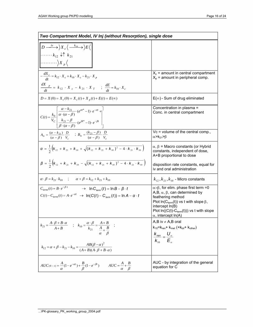
Two Compartment Model, IV Inj (without Resorption), single dose

p

kc

iv

X

kk

EXD

⋅⋅⋅⋅⋅⋅⋅⋅⋅⋅

↓↑⋅⋅⋅⋅⋅⋅⋅

⎯→⎯⎯→⎯

2112

10

pccc XkXkXk

dtdX

⋅−⋅+⋅=− 211012

Tcp XkXk

dtdX

⋅−⋅= 2112 ; cXkdtdE

⋅= 10

Xc = amount in central compartment Xp = amount in peripheral comp.

)()()()()0()0( ∞=++=== EtEtXtXXXD pcc E(∞) - Sum of drug eliminated

⎥⎥⎥⎥

⎦

⎤

⎢⎢⎢⎢

⎣

⎡

⋅−⋅−⋅−

+⋅−⋅−⋅

−

=−

−

tt

tt

C eek

eek

Vk

tCββ

αα

βαβββαα

α

)1()(

)1()(

)(*21

*21

0

Concentration in plasma = Conc. in central compartment

civ V

DkA ⋅−−

=)()( 21

βαα ;

civ V

DkB ⋅−−

=)()( 21

βαβ Vc = volume of the central comp.,

α>k21>β

( )10212

102112102112 421 kkkkkkkkα ⋅⋅−+++++= )(

( )10212

102112102112 421 kkkkkkkkβ ⋅⋅−++−++= )(

α, β = Macro constants (or Hybrid constants, independent of dose, A+B proportional to dose

disposition rate constants, equal for iv and oral administration

1021 kk ⋅=⋅ βα ; 102112 kkk ++=+ βα k k k12 21 10, , - Micro constants

tterm eBtC ⋅−⋅= β)( → tβBtCterm ⋅−= ln)(ln

tterm eAtCtC α−⋅=− )()( → tαAtCtC term ⋅−=− ln))()(ln(

α>β, for elim. phase first term =0 A,B, α, β, can determined by feathering method Plot ln(Cterm(t)) vs t with slope β, intercept ln(B) Plot ln((C(t)-Cterm(t))) vs t with slope α, intercept ln(A)

BABAk

+⋅+⋅

=αβ

21 ;

βα

βαBABA

kk

+

+=

⋅=

2110 ;

))((

)( 2

102112 αβαββα

⋅+⋅+−

=−−+=BABA

ABkkk

A,B iv ≠ A,B oral k10=kren+ kmet (+kbil+ kother)

∞

∞=EU

kkren

10

)1()1()0( ttt eBeAAUC βα

βα−−

− −+−= βαBAAUC +=

AUC - by integration of the general equation for C



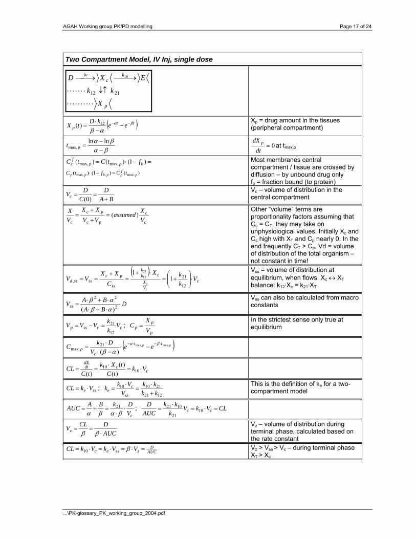
Two Compartment Model, IV Inj, single dose

p

kc

iv

X

kk

EXD

⋅⋅⋅⋅⋅⋅⋅⋅⋅⋅

↓↑⋅⋅⋅⋅⋅⋅⋅

⎯→⎯⎯→⎯

2112

10

( )ttp eekDtX βα

αβ−− −

−⋅

= 12)( Xp = drug amount in the tissues (peripheral compartment)

βαβα

−−

=lnln

max, pt 0=dt

dX p at tmax,p

=−⋅= )1()()( max,max, bppf

c ftCtC

)()1()( max,,max, pfppbpp tCftC =−⋅

Most membranes central compartment / tissue are crossed by diffusion – by unbound drug only fb = fraction bound (to protein)

BAD

CDVc +

==)0(

Vc – volume of distribution in the central compartment

c

c

pc

pc

c VX

assumedVVXX

VX )(=

+

+=

Other “volume” terms are proportionality factors assuming that Cc = CT, they may take on unphysiological values. Initially Xc and Cc high with XT and Cp nearly 0. In the end frequently CT > Cp. Vd = volume of distribution of the total organism – not constant in time!

( )c

VX

ckk

ss

pcssssd V

kkX

CXX

VVc

c⋅⎟⎟⎠

⎞⎜⎜⎝

⎛+=

⋅+=

+==

12

21, 1

112

21

Vss = volume of distribution at equilibrium, when flows Xc ↔ XT balance: k12·Xc = k21·XT

DBABAVss ⋅⋅+⋅⋅+⋅

= 2

22

)( αβαβ

Vss can also be calculated from macro constants

ccssp VkkVVV

12

21=−= ; p

pp V

XC =

In the strictest sense only true at equilibrium

( )pp tt

cp ee

VDkC max,max,

)(21

max,⋅−⋅− −⋅

−⋅⋅

= βα

αβ

ccdt

dEVk

tCtXk

tCCL ⋅=

⋅== 10

10

)()(

)(

sse VkCL ⋅= ; 1221

211010

kkkk

VVkk

ss

ce +

⋅=

⋅= This is the definition of ke for a two-

compartment model

cVDkBAAUC ⋅

⋅=+=

βαβα21 ; CLVkV

kkk

AUCD

cc =⋅=⋅

= 1021

1021

AUCDCLVz ⋅

==ββ

Vz – volume of distribution during terminal phase, calculated based on the rate constant

AUCD

zssec VVkVkCL =⋅=⋅=⋅= β10 Vz > Vss > Vc – during terminal phase XT > Xc



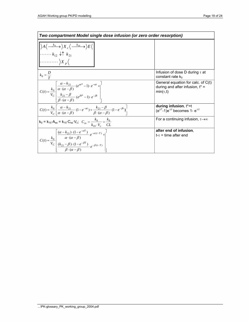
Two compartment Model single dose infusion (or zero order resorption)

p

kc

k

X

kk

EXA

⋅⋅⋅⋅⋅⋅⋅⋅⋅⋅⋅

↓↑⋅⋅⋅⋅⋅⋅⋅

⎯→⎯⎯→⎯

2112

100

TDk =0

Infusion of dose D during τ at constant rate k0

⎥⎥⎥⎥

⎦

⎤

⎢⎢⎢⎢

⎣

⎡

⋅−⋅−⋅−

+⋅−⋅−⋅

−

=−

−

tt

tt

C eek

eek

Vk

tCββ

αα

βαβββαα

α

)1()(

)1()(

)(*21

*21

0

General equation for calc. of C(t) during and after infusion, t* = min(τ,t)

⎥⎦

⎤⎢⎣

⎡−⋅

−⋅−

+−⋅−⋅

−= −− )1(

)()1(

)()( 21210 tt

Cekek

Vk

tC βα

βαββ

βααα

during infusion, t*=t (eλt*-1)e-λt becomes 1- e-λt

k0 = k10·Ass = k10·Css·Vc; CLk

Vkk

Cc

ss0

10

0 =⋅

= For a continuing infusion, τ→∞

⎥⎥⎥⎥⎥

⎦

⎤

⎢⎢⎢⎢⎢

⎣

⎡

⋅−⋅−⋅−

+⋅−⋅−⋅−

=−−

−

−−−

)(21

)(21

0

)()1()(

)()1()(

)(Tt

T

TtT

C eek

eek

Vk

tCβ

β

αα

βαββ

βααα

after end of infusion, t-τ = time after end



Two compartment Model, single dose with Resorption First Order

p

kc

k

X

kk

EXA a

⋅⋅⋅⋅⋅⋅⋅⋅⋅⋅⋅

↓↑⋅⋅⋅⋅⋅⋅⋅

⎯→⎯⎯→⎯

2112

10

⎥⎥⎥⎥

⎦

⎤

⎢⎢⎢⎢

⎣

⎡

⋅−⋅−

−+

⋅−⋅−

−+⋅

−⋅−−

⋅⋅⋅

=−

⋅−⋅

tk

aa

a

t

a

t

a

c

a

aekk

kk

ek

kek

k

VDFktC

)()()(

)()()(

)()()(

)(21

2121

βα

βαββ

ααβα βα

)()(

)()()()(

21

2121

aa

a

aa

kkkk

kk

kk

−⋅−−

−=

−⋅−−

+−⋅−

−

βα

ββαβ

ααβα

C-central compartment

with micro constants

tktt aeBAeBeAtC −⋅−⋅− ⋅+−⋅+⋅= )()( βα

C-central compartment

with macro constants

)()( 21

αβα

−−

⋅=k

VDA

cIV ;

)()( 21

βαβ

−−

⋅=k

VDB

cIV

iva

aoral A

kfkA ⋅

−⋅

=)( α

; iva

aoral B

kfkB ⋅

−⋅

=)( β

iviv

c

BfAfD

fV

⋅+⋅=

Without iv data only Vc/f can be determined, but based on knowledge of f⋅Aiv and f⋅Biv the micro constants k10, k21, k12 may be derived

tk

a

ttp

aekkkBAe

kkBe

kkAtC −−− ⋅

−⋅+

−−⋅

+⋅−⋅

=)(

)()()(

)(21

21

21

21

21

21 βα

βα

CT-deep compartment

Two compartment Model, multiple dose with Resorption First Order

xa

a

a

xx

tkk

nk

tntn

xn

eeeBA

eeeBe

eeAtC

−−

−

−−

−−

−

−

−−

+−

−−

+⋅−−

⋅=

τ

τ

ββτ

βτα

ατ

ατ

11)(

11

1)1()(

Cn – concentration at time tx after the nth administration at interval τ, time after first dosing = n⋅τ



3 PHARMACODYNAMIC GLOSSARY

3.1 Definitions

Symbol Unit / Dimension Definition

AUEC Arbitrary units·time Area under the effect curve

Ce Amount/volume Fictive ‘concentration’ in the effect compartment

Cp Amount/volume Drug concentration in the central compartment

E (effect unit) Effect

E0 (effect unit) Baseline effect

Emax (effect unit) Maximum effect

EC50 Amount/volume Drug concentration producing 50% of maximum effect

Imax (effect unit) Maximum inhibition

I50 Amount/volume Drug concentration producing 50% of maximal inhibition

keo (Time)-1 Rate constant for degradation of the effect compartment

kin (effect unit) (time)-1 Zero order constant for input or production of response

kout (time)-1 First order rate constant for loss of response

M50 Amount/volume 50% of maximum effect of the regulator

MEC Amount/volume Minimum effective concentration

n - Sigmoidicity factor (Hill exponent)

S (effect unit)/

(amount/volume)

Slope of the line relating the effect to the concentration

tMEC Time Duration of the minimum (or optimum) effective concentration

Ve Volume Fictive volume of the effect compartment



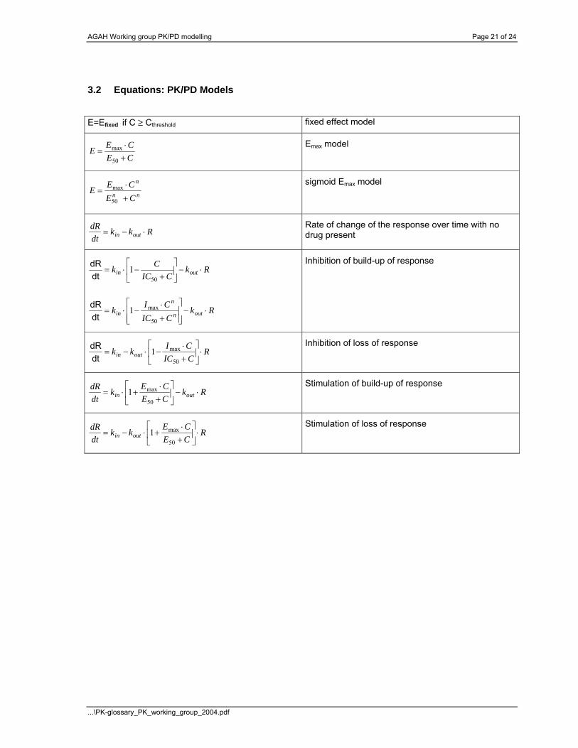
3.2 Equations: PK/PD Models

E=Efixed if C ≥ Cthreshold fixed effect model

CECE

E+⋅

=50

max Emax model

nn

n

CECE

E+

⋅=

50

max sigmoid Emax model

RkkdtdR

outin ⋅−= Rate of change of the response over time with no drug present

RkCIC

Ck outin ⋅−⎥⎦

⎤⎢⎣

⎡+

−⋅=50

1dtdR

RkCICCI

k outn

n

in ⋅−⎥⎥⎦

⎤

⎢⎢⎣

⎡

+

⋅−⋅=

50

max1dtdR

Inhibition of build-up of response

RCICCI

kk outin ⋅⎥⎦

⎤⎢⎣

⎡+⋅

−⋅−=50

max1dtdR

Inhibition of loss of response

RkCECE

kdtdR

outin ⋅−⎥⎦

⎤⎢⎣

⎡+⋅

+⋅=50

max1 Stimulation of build-up of response

RCECE

kkdtdR

outin ⋅⎥⎦

⎤⎢⎣

⎡+⋅

+⋅−=50

max1 Stimulation of loss of response



4 STATISTICAL PARAMETERS 4.1 Definitions

Symbol Definition Calculation

AIC Akaike Information Criterion

(smaller positive values indicate a better fit) AIC = n·ln(WSSR) +2p

n = number of observed (measured) concentrations, p = number of parameters in the model

CI Confidence interval, e.g. 90%-CI SEMtxCI n ⋅±= − α,1

CV Coefficient of variation in %

xSD⋅100= CV , SD = standard deviation

Median = ~x

Median, value such that 50% of observed values are below and 50% above

(n+1)st value if there are 2n+1 values or arithmetic mean of nth and (n+1)st value if there are 2n values

Mean = x Arithmetic mean ∑=

=n

iix

nx

1

1

MSC Model selection criterion AIC, SC, F-ratio test, Imbimbo criterion etc.

SC Schwarz criterion SC = n·ln(WSSR) +p·ln(n)

SD Standard deviation VarSD =

SEM Standard error of mean

nSDSEM =

SSR Sum of the squared deviations between the calculated values of the model and the measured values ( )∑

n

1=iC -

,, = SSR

calciobsiC

2

SS Sum of the squared deviations between the measured values and the mean value C ( )∑

n

1=iC -

, = SS

obsiC

2

n - = SS

,

,

2

1

1

2⎟⎟⎠

⎞⎜⎜⎝

⎛

⎟⎟⎠

⎞⎜⎜⎝

⎛ ∑∑ =

=

n

iobsin

iobsi

CC

n = number of observed (measured) concentrations

use of the second formula is discouraged although mathematically identical

WSS or WSSR Weighted sum of the squared deviations between the calculated values of the model and the measured values

( )∑n

1=iC -

,, = WSSR

calciobsiCiw

2

Var Variance s² = SS/(n-1)

X25% Lower quartile (25%- quantile), value such that 25% of observed values are below and 75% above

may be calculated as median of values between minimum and the overall median

X75% Upper quartile (75%- quantile) may be calculated as median of values between the overall median and the maximum



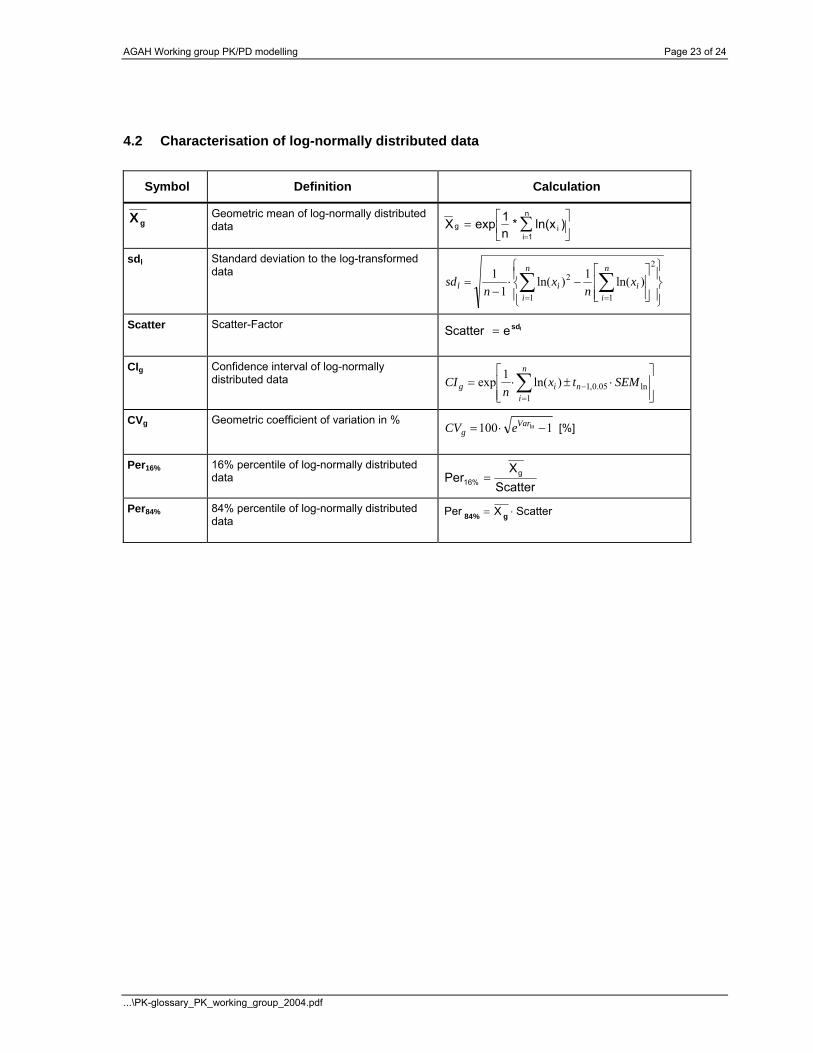
4.2 Characterisation of log-normally distributed data

Symbol Definition Calculation

gX

Geometric mean of log-normally distributed data ⎥

⎦⎤

⎢⎣⎡= ∑

=

n

1iig )ln(x*

n1expX

sdl Standard deviation to the log-transformed data

⎪⎭

⎪⎬⎫

⎪⎩

⎪⎨⎧

⎥⎥⎦

⎤

⎢⎢⎣

⎡−⋅

−= ∑ ∑

= =

n

i

n

iiil x

nx

nsd

1

2

1

2 )ln(1)ln(1

1

Scatter Scatter-Factor lsdeScatter =

CIg Confidence interval of log-normally distributed data

⎥⎥⎦

⎤

⎢⎢⎣

⎡⋅±⋅= ∑

=−

n

inig SEMtx

nCI

1ln05.0,1)ln(1exp

CVg Geometric coefficient of variation in % 1100 ln −⋅= Var

g eCV [%]

Per16% 16% percentile of log-normally distributed data

ScatterX

Per g16% =

Per84% 84% percentile of log-normally distributed data

ScatterXPer g84% ⋅=

collection of terms, symbols, equations, and explanations of … · glossary page 2 of...

Documents