colour image processing · colour image processing 7.2 segmentation in rgb colour space given a set...

Digital Image Processing

© 1992–2008 R. C. Gonzalez & R. E. Woods

T. Peynot

Chapter 5

Colour Image Processing


1. Colour Fundamentals

2. Colour Models

3. Pseudocolour Image Processing

4. Basics of Full-Colour Image Processing

5. Colour Transformations

6. Smoothing and Sharpening

7. Image Segmentation based on Colour



T. Peynot

Chapter 5


Motivation to use colour:

• Powerful descriptor that often simplifies object identification and extraction

from a scene

• Humans can discern thousands of colour shades and intensities, compared to

about only two dozen shades of gray

Two major areas:

• Full-colour processing: e.g. images acquired by colour TV camera or colour

scanner

• Pseudo-colour processing: assigning a colour to a particular monochrome

intensity or range of intensities

Some of the gray-scale methods are directly applicable to colour images

Others require reformulation

Introduction



T. Peynot

Chapter 5


1. Colour Fundamentals



T. Peynot

Chapter 5


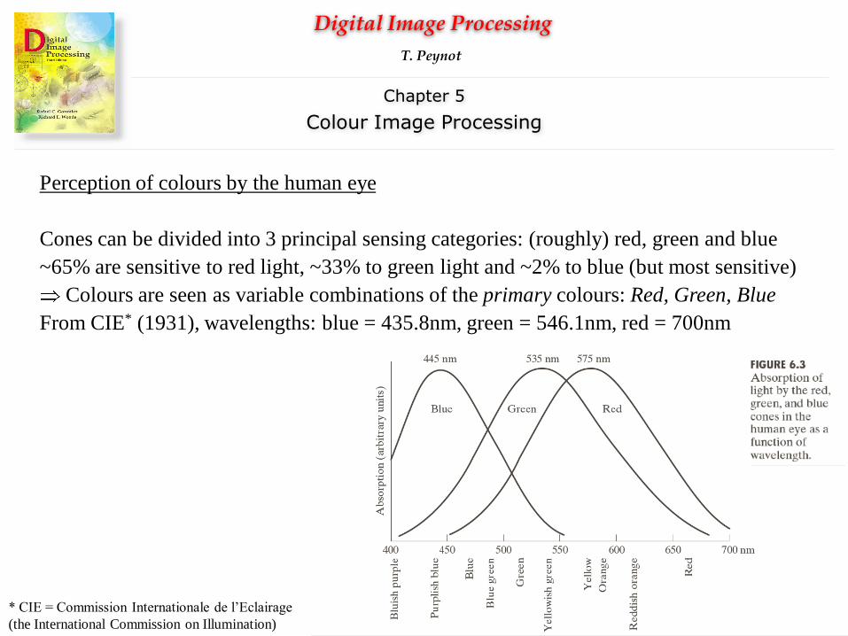
Perception of colours by the human eye

Cones can be divided into 3 principal sensing categories: (roughly) red, green and blue

~65% are sensitive to red light, ~33% to green light and ~2% to blue (but most sensitive)

Colours are seen as variable combinations of the primary colours: Red, Green, Blue

From CIE* (1931), wavelengths: blue = 435.8nm, green = 546.1nm, red = 700nm

* CIE = Commission Internationale de l’Eclairage

(the International Commission on Illumination)



T. Peynot

Chapter 5


Primary colours can be added to produce

the secondary colours of light:

• Magenta (red plus blue)

• Cyan (green plus blue)

• Yellow (red plus green)

Mixing the three primaries in the right

intensities produce white light

Primary colours of pigment: absorb a

primary colour of light and reflects or

transmits the other two

magenta, cyan and yellow



T. Peynot

Chapter 5


Characteristics of a colour:

• Brightness: embodies the achromatic notion of intensity

• Hue: attribute associated with the dominant wavelength in a mixture of light waves

• Saturation: refers to the relative purity or the amount of white light mixed with a hue

(The pure spectrum colours are fully saturated; e.g. Pink (red and white) is less

saturated, degree of saturation being inversely proportional to the amount of white light

added)

Hue and Saturation together = chromaticity

Colour may be characterized by its brightness and chromaticity



T. Peynot

Chapter 5


Tristimulus values = amounts of red (X), green (Y) and blue (Z) needed to form a

particular colour. A colour can be specified by its trichromatic coefficients:

NB:



T. Peynot

Chapter 5


Another approach for specifying colours:

The CIE chromaticity diagram:

Shows colour composition as a function of x (red)

and y (green)

Content:

62% green

25% red

13% blue

Pure colours of the spectrum (fully saturated):

boundary

Equal fractions of the 3

primary colours (CIE

standard for white light)

For any value of x and y: z (blue) is obtained

by:



T. Peynot

Chapter 5


Typical range of colours (colour gamut) produced by RGB monitors:

Colour gamut of today’s high-

quality colour printing devices



T. Peynot

Chapter 5


2. Colour Models

• Also called: colour spaces or colour systems

• Purpose: facilitate the specification of colours in some “standard” way

• Colour model = specification of a coordinate system and a subspace within it where

each colour is represented by a single point

Most commonly used hardware-oriented models:

• RGB (Red, Green, Blue), for colour monitors and video cameras

• CMY (Cyan, Magenta, Yellow) and CMYK (CMY+Black) for colour printing

• HSI (Hue, Saturation, Intensity)



T. Peynot

Chapter 5


2.1 The RGB Colour Model

• Each colour appears in its primary spectral components of Red, Green and Blue

• Model based on a Cartesian coordinate System

• Colour subspace = cube

• RGB primary values: at 3 opposite corners (+ secondary values at 3 others)

• Black at the origin, White at the opposite corner

Convention: all colour values normalized

=> unit cube and all values of R,G,B in [0,1]

Gray scale



T. Peynot

Chapter 5


Number of bits used to represent each pixel in the RGB space = pixel depth

Example: RGB image in which each of the red, green and blue images is a 8-bit image

Each RGB colour pixel (i.e. triplet of values (R,G,B)) is said to have a depth of 24

bits (full-colour image)

Total number of colours in a 24-bit RGB image is: (28)3 = 16,777,276



T. Peynot

Chapter 5


NB: acquiring an image = reversed process:

Using 3 filters sensitive to red, green and blue, respectively (e.g. Tri-CCD sensor)



T. Peynot

Chapter 5


Colour Image acquisition: Colour MonoCCD and Bayer Filter Mosaic

Bayer Mosaic Diagonal Mosaic Columns Mosaic

[Aviña Cervantes 2005]



T. Peynot

Chapter 5


“Demosaicking”: Interpolating the values of missing pixels in the component images

Example:

• Bilinear demosaicking:




T. Peynot

Chapter 5


Other methods :

• Nearest Neighbour Method

• Demosaicking by median filter

• Demosaicking by constant hue

• Demosaicking by gradients detection

• Adaptive interpolation by Laplacian

“Demosaicking”




T. Peynot

Chapter 5


2.2 XYZ (CIE)

• Official definition of the CIE XYZ standard (normalised matrix):

• Commonly used form: w/o leading fraction => RGB=(1,1,1) Y=1



T. Peynot

Chapter 5


2.2 The CMY and CMYK Colour Models

CMY: Cyan, Magenta, Yellow (secondary colours of light, or primary colours of

pigments)

• CMY data input needed by most devices that deposit coloured pigments on paper,

such as colour printers and copiers

• or RGB to CMY conversion:

(assuming normalized colour values)

Equal amounts of cyan, magenta and yellow => black, but muddy-looking in practice

=> To produce true black (predominant colour in printing) a 4th colour, black, is added

=> CMYK model (CMY + Black)



T. Peynot

Chapter 5


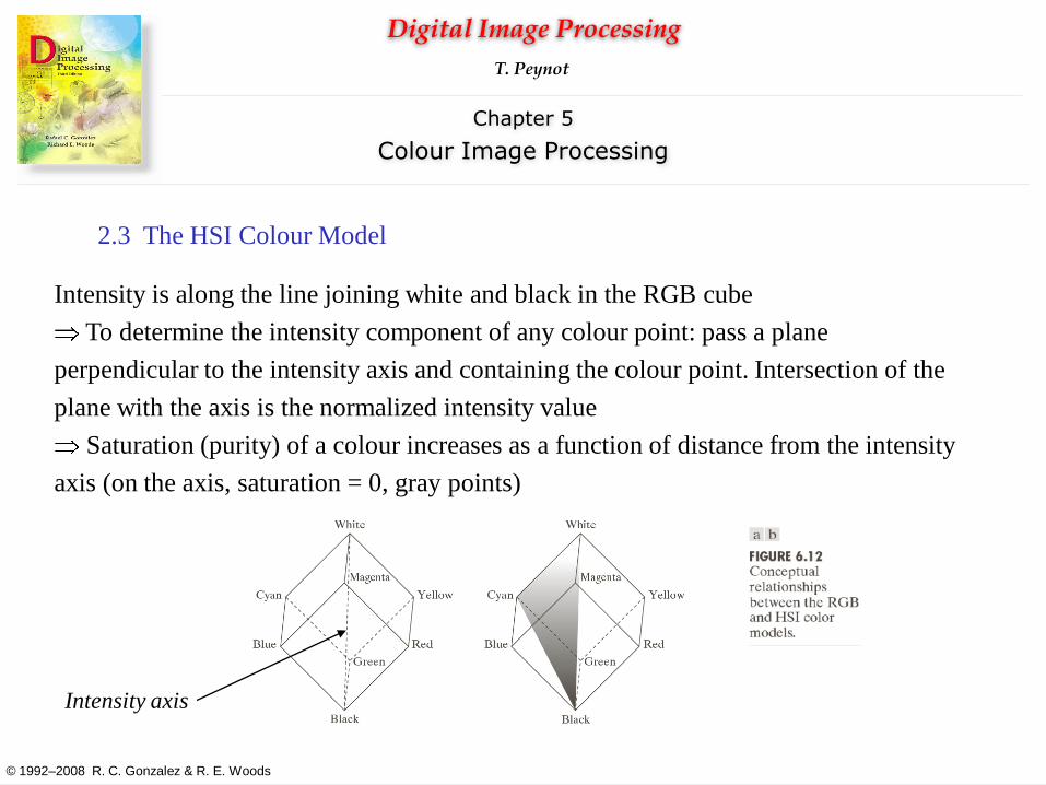
2.3 The HSI Colour Model

RGB and CMY models: straightforward + ideally suited for hardware implementations

+ RGB system matches nicely the human eye perceptive abilities

But, RGB and CMY not well suited for describing colours in terms practical for human

interpretation

Human view of a colour object described by Hue, Saturation and Brightness (or Intensity)

• Hue: describes a pure colour (pure yellow, orange or red)

• Saturation: gives a measure of the degree to which a pure colour is diluted by white light

• Brightness: subjective descriptor practically impossible to measure. Embodies the

achromatic notion of intensity => intensity (gray level), measurable

=> HSI (Hue, Saturation, Intensity) colour model

(or HSL: Lightness, HSB: Brightness, HSV: Value)



T. Peynot

Chapter 5


2.3 The HSI Colour Model

Intensity is along the line joining white and black in the RGB cube

To determine the intensity component of any colour point: pass a plane

perpendicular to the intensity axis and containing the colour point. Intersection of the

plane with the axis is the normalized intensity value

Saturation (purity) of a colour increases as a function of distance from the intensity

axis (on the axis, saturation = 0, gray points)

Intensity axis



T. Peynot

Chapter 5


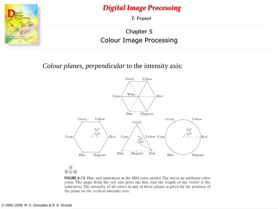
Colour planes, perpendicular to the intensity axis:



T. Peynot

Chapter 5


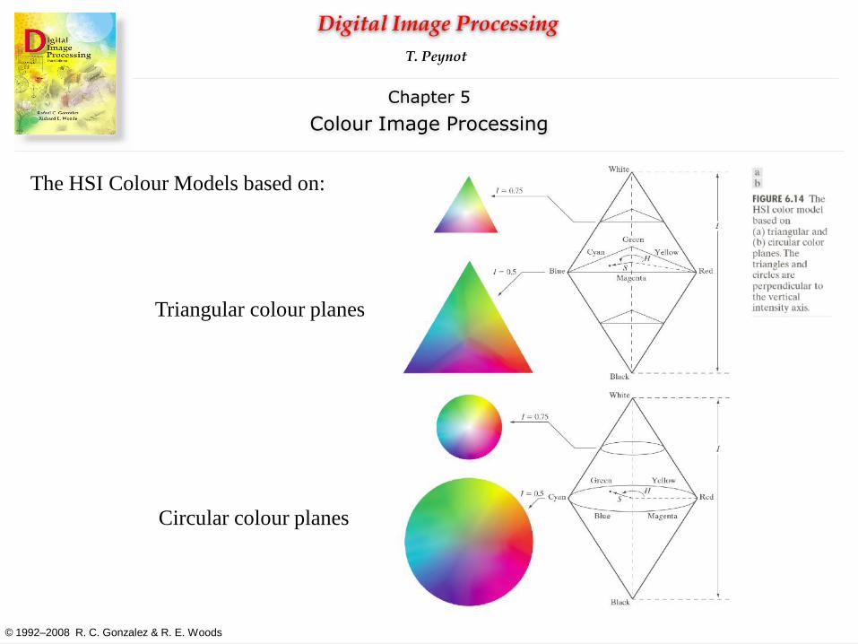
The HSI Colour Models based on:

Triangular colour planes

Circular colour planes



T. Peynot

Chapter 5


Conversion from RGB to HSI

Given an RGB pixel:

with

Saturation:

Intensity: NB: RGB values normalised to [0,1],

Theta measured w.r.t. red axis of the HSI space

then normalise H



T. Peynot

Chapter 5


Conversion from HSI to RGB

Three sectors of interest:

• RG sector (0 H 120 ):

• GB sector (120 H 240 ):



T. Peynot

Chapter 5


• BR sector (240 H 360 ):


• Then normalise H



T. Peynot

Chapter 5


RGB 24-bit colour cube Corresponding HSI values

=>


Hue Saturation Intensity



T. Peynot

Chapter 5


Primary and secondary

RGB colours H

S I

Manipulation of HSI images:



T. Peynot

Chapter 5


H S

I RGB

image

Manipulation of HSI images: H

S

I

I

Original image

Modified HSI image



T. Peynot

Chapter 5


2.4 The L*a*b* model

Example of Colour Management System (CMS):

CIE L*a*b* model, or CIELAB:

Where:

XW, YW and ZW are reference white tristimulus



T. Peynot

Chapter 5


The L*a*b* colour space is:

• Colorimetric (colours perceived as matching are encoded identically)

• Perceptually uniform (colour differences among various hues are perceived

uniformly)

• Device independent

Other characteristics:

• Not a directly displayable format

• Its gamut encompasses the entire visible spectrum

• Can represent accurately the colours of any display, print, or input device

• Like HSI, excellent decoupler of intensity (represented by lightness L*) and

colour (a* for red minus green, b* for green minus blue)



T. Peynot

Chapter 5



2 major categories:

• Processing of each component image individually

=> composite processed colour image

• Work with colour pixels (vectors) directly

Vector in RGB colour space:



T. Peynot

Chapter 5



Per-colour-component and vector-based processing equivalent iff:

1. The process is applicable to both vectors and scalars

2. The operation on each component of a vector is independent of the other

components



T. Peynot

Chapter 5


5. Colour Transformations

NB: Context of a single colour model (no conversion between models)

5.1 Formulation

Colour input image (processed) colour

output image

Operator defined over a

spatial neighbourhood of

point (x,y)

(cf. 3.1)

Basic transformations:

e.g. RGB or HSI: n=3. CMYK: n=4

Set of transformation of colour mapping functions



T. Peynot

Chapter 5




T. Peynot

Chapter 5


Example: modify the intensity of the full-colour image using:

In HSI:

In RGB:

In CMY:



T. Peynot

Chapter 5


5.2 Colour complements

Hues directly opposite one another on the colour circle = complements

Complements are analogous to gray-scale negatives (section 3.2.1)

Useful for enhancing detail embedded in dark regions



T. Peynot

Chapter 5


5.2 Colour complements



T. Peynot

Chapter 5


5.3 Colour slicing

Highlighting a specific range of colours to separate objects from surroundings

• Display the colour of interest, or:

• Use the region defined by colours as a mask

If colours of interest enclosed by a cube (or hypercube) of width W and centered at a

prototypical (e.g. average) colours with components (a1, a2,…, an), then:

=> Highlight the colours around the prototype by forcing all other colours to the

midpoint of the reference colour space (e.g. middle gray in RGB: (0.5,0.5,0.5))



T. Peynot

Chapter 5


5.3 Colour slicing

=>



T. Peynot

Chapter 5


5.4 Tone and Colour Corrections

Effectiveness of these transformations judged ultimately in print

But developed, refined and evaluated on monitors

Need to maintain a high degree of colour consistency between monitors used and

eventual output devices

Device-independent colour model, relating the colour gamuts of the monitors

and output devices



T. Peynot

Chapter 5


Boosting contrast

Cf. power-law

transformations

1. Tonal transformations

Typical transformations for correcting

three common tonal imbalances:



T. Peynot

Chapter 5


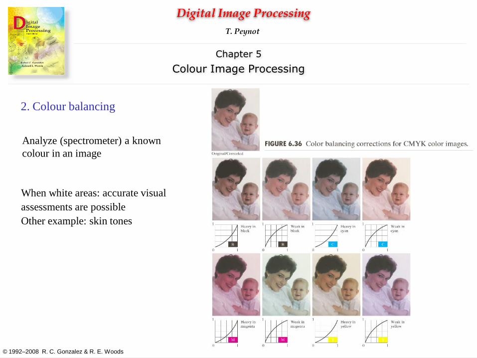
2. Colour balancing

• Goal: move the white point of a given image closer to pure white

(R=G=B)

• Example of strongly coloured illuminant: incandescent indoor lighting

(=> yellow or orange hue)

• NB: using white may not always be a good idea…



T. Peynot

Chapter 5


2. Colour balancing

Analyze (spectrometer) a known

colour in an image

When white areas: accurate visual

assessments are possible

Other example: skin tones



T. Peynot

Chapter 5


44

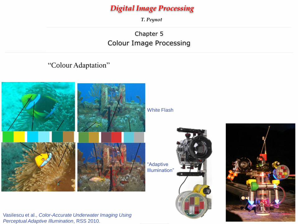
White Flash

Vasilescu et al., Color-Accurate Underwater Imaging Using

Perceptual Adaptive Illumination, RSS 2010.

“Adaptive

Illumination”

“Colour Adaptation”



T. Peynot

Chapter 5


5.5 Histogram Processing

Example: Histogram Equalisation in the HSI colour space



T. Peynot

Chapter 5


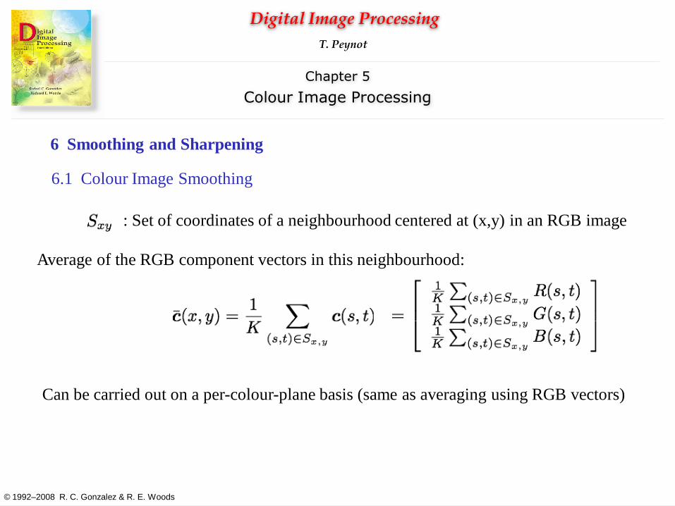
6 Smoothing and Sharpening

6.1 Colour Image Smoothing

: Set of coordinates of a neighbourhood centered at (x,y) in an RGB image

Average of the RGB component vectors in this neighbourhood:

Can be carried out on a per-colour-plane basis (same as averaging using RGB vectors)



T. Peynot

Chapter 5


Colour Image Smoothing: Example

RGB

G B

R



T. Peynot

Chapter 5


H S I

Colour Image Smoothing: Example RGB



T. Peynot

Chapter 5


Smoothing each RGB

component image Smoothing the I of HSI Difference

Colour Image Smoothing: Example



T. Peynot

Chapter 5


6.1 Colour Image Sharpening

In RGB, the Laplacian of vector c is:

=> Can be computed on each component image separately



T. Peynot

Chapter 5


Original image

Hue

Saturation Intensity

Binary saturation mask

(threshold=10% of max value) Mask * Hue image

7 Image Segmentation Based on Colour

7.1 Segmentation in HSI Colour Space

Example:

Typically: segmentation on

Hue image



T. Peynot

Chapter 5


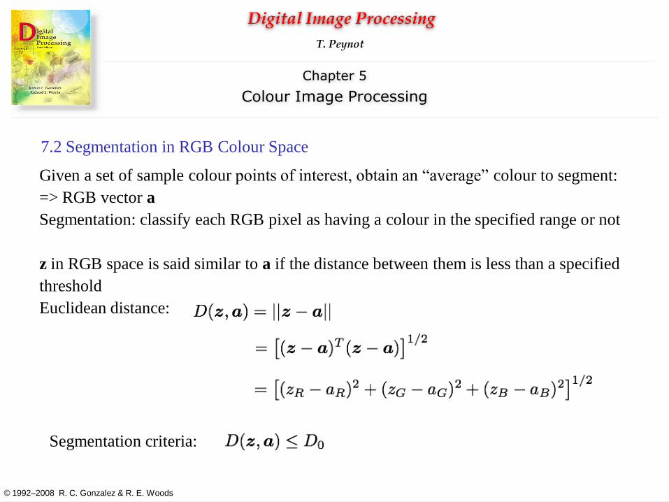
7.2 Segmentation in RGB Colour Space

Given a set of sample colour points of interest, obtain an “average” colour to segment:

=> RGB vector a

Segmentation: classify each RGB pixel as having a colour in the specified range or not

z in RGB space is said similar to a if the distance between them is less than a specified

threshold

Euclidean distance:

Segmentation criteria:



T. Peynot

Chapter 5


7.2 Segmentation in RGB Colour Space

Generalization of the distance measure:

Where C is the covariance matrix of the samples representative of the colour we

wish to segment

Euclidean

distance

Generalized

distance

Bounding box

(Mahalanobis distance)



T. Peynot

Chapter 5


Example:

1. Compute mean vector a of colour points

in rectangle

2. Compute the standard deviation of red,

green and blue values

3. Box centered on a, dimensions along

each RGB axes: 1.25 R



T. Peynot

Chapter 5


References:

• R.C. Gonzalez and R.E. Woods, Digital Image Processing, 3rd Edition, Prentice Hall, 2008

• D.A. Forsyth and J. Ponce, Computer Vision – A Modern Approach, Prentice Hall, 2003

• J.G. Aviña Cervantes, Navigation visuelle d'un robot mobile dans un environnement

d'extérieur semi-structuré (Visual Navigation of a Mobile Robot in semi-structured outdoor

environment), PhD Thesis, Institut National Polytechnique de Toulouse, 2005

colour image processing · colour image processing 7.2 segmentation in rgb colour space given a set...

Documents