combined use of optical and radar satellite data for the

Hydrol. Earth Syst. Sci., 15, 1117–1129, 2011www.hydrol-earth-syst-sci.net/15/1117/2011/doi:10.5194/hess-15-1117-2011© Author(s) 2011. CC Attribution 3.0 License.

Hydrology andEarth System

Sciences

Combined use of optical and radar satellite data for the monitoringof irrigation and soil moisture of wheat crops

R. Fieuzal1, B. Duchemin1, L. Jarlan1, M. Zribi 1, F. Baup1, O. Merlin 1, O. Hagolle1, and J. Garatuza-Payan2

1CESBIO, Centre d’etudes spatiales de la biosphere, UMR 5126, CNES-CNRS-IRD-UPS, Toulouse, France2ITSON, Instituto Tecnologico de Sonora, Departamento de Ciencias del Agua y del Medio Ambiente, 5 de Febrero 818 Sur,Cd. Obregon, Sonora, 85000, Mexico

Received: 22 July 2010 – Published in Hydrol. Earth Syst. Sci. Discuss.: 25 August 2010Revised: 11 March 2011 – Accepted: 17 March 2011 – Published: 5 April 2011

Abstract. The objective of this study is to get a better un-derstanding of radar signal over irrigated wheat fields and toassess the potentialities of radar observations for the moni-toring of soil moisture. Emphasis is put on the use of highspatial and temporal resolution satellite data (Envisat/ASARand Formosat-2). Time series of images were collected overthe Yaqui irrigated area (Mexico) throughout one agriculturalseason from December 2007 to May 2008, together withmeasurements of soil and vegetation characteristics and agri-cultural practices. The comprehensive analysis of these dataindicates that the sensitivity of the radar signal to vegetationis masked by the variability of soil conditions. On-going ir-rigated areas can be detected all over the wheat growing sea-son. The empirical algorithm developed for the retrieval oftopsoil moisture from Envisat/ASAR images takes advantageof the Formosat-2 instrument capabilities to monitor the sea-sonality of wheat canopies. This monitoring is performedusing dense time series of images acquired by Formosat-2 toset up the SAFY vegetation model. Topsoil moisture esti-mates are not reliable at the timing of plant emergence andduring plant senescence. Estimates are accurate from tiller-ing to grain filling stages with an absolute error about 9%(0.09 m3 m−3, 35% in relative value). This result is attractivesince topsoil moisture is estimated at a high spatial resolution(i.e. over subfields of about 5 ha) for a large range of biomasswater content (from 5 and 65 t ha−1) independently from theviewing angle of ASAR acquisition (incidence angles IS1 toIS6).

Correspondence to:R. Fieuzal([email protected])

1 Introduction

Effective management and monitoring of environmental re-sources require integrating hydro-ecologic parameters intobiophysical models. However, although models perfor-mances have continuously been improved over the past years,regional applications for the management of agricultural wa-ter are still limited because of the shortage of key input mod-elling data over large areas (Boote et al., 1996; Moulin etal., 1998; Faivre et al., 2004). The monitoring of farmingpractices and soil-vegetation biophysical variables combin-ing modeling and remote sensing data offers both advan-tages. On one hand, punctual parameters derived from satel-lite acquisition can be used as input to constrain models. Onother hand, the continuous and spatialized modeled variablescan be used to improve the knowledge on the informationderived from remote sensing data.

Recently designed earth observing systems offer both highspatial resolution and frequent revisit time. This is particu-larly promising for the seasonal monitoring of croplands ata field scale. At the present time, the Formosat-2 satelliteprovides 8 m resolution images (in the multispectral modeat nadir viewing) for 4 narrow spectral bands ranging from0.45 µm to 0.90 µm (blue, green, red and near-infrared). Itis a unique tool to monitor the seasonality of biophysicalvariables such as leaf area index (Duchemin et al., 2008a;Bsaibes et al., 2009; Hadria et al., 2009a). In the microwavespectral domain, the ASAR radar onboard the Envisat mis-sion is an active instrument operating at C-band with a 30m spatial resolution in the Alternating Polarisation mode.The orbit cycle is 35 days, but the combination of acquisi-tions at different incidence angles allows revisiting of a fewdays (Torres et al., 1999). The continuity of combined high

Published by Copernicus Publications on behalf of the European Geosciences Union.

http://creativecommons.org/licenses/by/3.0/

1118 R. Fieuzal et al.: Combined use of optical and radar satellite data

resolution and repetitivity data sets in the microwave and theoptical spectral domains is insured in the near future by theplanned launch of Sentinel-1 and Sentinel-2 satellite mis-sions (ESA, 2007, cited in Hagolle et al., 2008).

Optical satellite data were intensively used in the contextof crop monitoring to provide space and time regular obser-vations of plant biophysical variables (Asrar et al., 1984;Baret and Guyot, 1991; Carlson and Ripley, 1997; Basti-aanssen et al., 2000; Duchemin et al., 2006). In contrast,there is still a poor understanding of the radar response overannual crops (Moran et al., 2002). For wheat canopies,the sensitivity of the radar backscattering co-polarization ra-tio is caused by the differential attenuation of horizontallyand vertically polarized electromagnetic waves that propa-gate through a medium with vertical structure (Bracaglia etal., 1995; Picard et al., 2003). Some attempts at using empir-ical relationships between Envisat/ASAR backscattering co-efficient and wheat leaf area index characteristics have beenperformed (Dente et al., 2008). The limitation of these meth-ods lies in the saturation of the signal with the density ofcanopies and its sensitivity to surface roughness and topsoilmoisture (Moran et al., 2002; Mattia et al., 2003; Ulabyet al., 1986; Beaudoin et al., 1990; Satalino et al., 2003;Zribi et al., 2003). The general trends of the radar responseas a function of soil conditions and the sensor characteris-tics (frequency, incidence, polarisation) are well captured bybackscatter models (e.g. Jarlan et al., 2002), but the opera-tional applicability of inversion schemes is still challengingsince the parameters required for modelling are difficult toestimate over large areas and since the relative contributionof these parameters on the signal is difficult to decouple.

In this context, the objective of this study is twofold: (i) toget a better understanding of radar signal over irrigated wheatfields and, (ii) to show the potentialities of radar observa-tions for the monitoring of irrigation and soil moisture. Thestudy is carried out over an irrigated area located in North-West of Mexico (arid climate with 200 mm of rain per year).Emphasis is put on time series of high spatial resolution im-ages (30 m) provided by Envisat/ASAR. The potentialities ofthese data for the monitoring of soil conditions is analysedbased on spatial estimates of Biomass Water Content (BWC).These estimates are obtained over a large number of fields us-ing a simple wheat growth model controlled by Formosat-2data. The analysis of the covariations of backscattering co-efficients and BWC shows the high sensitivity of the radarresponse to the irrigation status. It allowed developing anoriginal method for the retrieval of topsoil moisture basedon the spatial variation of backscattering coefficients under alarge range of vegetation growing stage.

Figure 1. The 8×8 km² study area delineated on a Formosat-2 image, with its 4×4 km² central part

highlighted. Wheat fields are hatched in black. Agricultural practices were collected on 12 wheat

fields (beige fields). The bottom zoomed yellow area shows the largest fields where grain yield

(green subfields) and irrigation (black segments) were collected.

8 km

4 km

N

Fig. 1. The 8×8 km2 study area delineated on a Formosat-2 image,with its 4×4 km2 central part highlighted. Wheat fields are hatchedin black. Agricultural practices were collected on 12 wheat fields(beige fields). The bottom zoomed yellow area shows the largestfields where grain yield (green subfields) and irrigation (black seg-ments) were collected.

2 Overview of the experiment

2.1 Study area

The experiment was conducted throughout one agriculturalseason from November 2007 to June 2008 in the Yaqui Val-ley, North-West of Mexico (27.25◦ N, 109.88◦ W). The ob-jective of the experiment was to characterize the spatial vari-ability of surface fluxes from the field to regional (few km)scale. Field measurements were collected on an 8×8 km2

irrigated cropping area where land use was exhaustively col-lected (Fig. 1). Wheat was the dominant crop covering 60%of the study area.

The study area is adequate to get a better understanding ofthe radar signal over wheat fields since: (i) it is flat, thus radarbackscattering is not influenced by topography, (ii) fields arelarge (up to 100 ha), with only two different North-South andEast-West row orientations, (iii) agricultural practices are al-most identical for all the wheat fields: mechanized tillage,irrigation and fertilization operations applied in the course ofprogrammed schedules.

Hydrol. Earth Syst. Sci., 15, 1117–1129, 2011 www.hydrol-earth-syst-sci.net/15/1117/2011/

R. Fieuzal et al.: Combined use of optical and radar satellite data 1119

Figure 2. Picture taken on the largest field at the irrigation limit (before sowing). Fig. 2. Picture taken on the largest field at the irrigation limit(before sowing).

2.2 Experimental data

Wheat fields located in the 4× 4 km2 central part of the8×8 km2 area were intensively monitored during the exper-iment. Climatic data, agricultural practices, vegetation andsoil biophysical variables were collected regularly during allthe agricultural season.

Climatic data were collected by a meteorological stationinstalled at the center of the study area between 27 Decem-ber 2007 and 17 May 2008. Air temperature and solar radi-ation were collected at a semi-hourly time step, from whichdaily mean air temperature average and daily accumulatedglobal incoming radiation were computed.

Agricultural practices were collected on 12 wheat fieldslocated within the 4×4 km2 centre (see Fig. 1). Sowing andirrigation dates are used in this study. Sowing period wasfrom 25 November 2007 and 8 January 2008, with a pre-irrigation performed to prepare the seedling. After sowing,wheat crops were irrigated 3 to 4 times. Furrow irrigationwas used (Fig. 2), with a water quantity of 150 mm each time.Harvesting was performed from April end to May.

Vegetation measurements consist in Green Leaf Area in-dex (GLA) and Grain Yield (GY) estimates. GLA data werederived from hemispherical photography taken on 20×20 m2

plot following the VALERI protocol (Garrigues et al., 2006)based on the analysis of canopy directional gap fraction. Atthe end of the season, grain yield was estimated on 11 fieldsby surveying harvesting machine with GPS system on trackmode (see the zoomed part in Fig. 1).

Topsoil moisture was measured using TDR sensors in-stalled within 2 pits, at 5 cm depth. During the agriculturalseason, data were collected on 2 wheat fields at a semi-hourly time step. These measurements were calibrated andtransformed in volumetric soil moisture by comparison withgravimetric measurements. The values the closest to ASARacquisition dates are used in this study; the time gap betweensatellite acquisitions and in situ measurements never exceeds15 min.

Figure 3. Satellite acquisition dates (× Formosat-2, + Envisat/ASAR) together with the main

phenological stages of wheat crops. The ASAR acquisition mode is indicated (top number:

ascending overpass; bottom number: descending overpass; the number indicates the

illumination/viewing angle from IS1 to IS6).

Fig. 3. Satellite acquisition dates (× Formosat-2, + Envisat/ASAR)together with the main phenological stages of wheat crops. TheASAR acquisition mode is indicated (top number: ascending over-pass; bottom number: descending overpass; the number indicatesthe illumination/viewing angle from IS1 to IS6).

2.3 Remote sensing data

Two series of satellite acquisitions were specifically pro-grammed during the experiment. The acquisition dates areshown in Fig. 3, together with the phenological main phasesand agricultural operations for wheat crops. 37 optical im-ages were acquired by the Formosat-2/RSI sensor, from15 November 2007 to 6 June 2008. 43 radar images wereacquired by the Envisat/ASAR sensor, from 1 January 2008to 2 June 2008. The main characteristics of these images andtheir preprocessing are detailed below.

2.3.1 Formosat-2 data

The Formosat-2 Taiwanese satellite was launched inMay 2004. The remote sensing instrument onboardFormosat-2 provides high spatial resolution images (8 m inthe multispectral mode at nadir viewing) in four narrow spec-tral bands ranging from 0.45 µm to 0.90 µm (blue, green, redand near-infrared). Unlike other systems operating at highspatial resolution, Formosat-2 may observe a particular areaevery day with the same viewing angle. However, only apart – about the half – of the Earth may be observed. Moredetails about the specific orbital cycle and other characteris-tics of the Formosat-2 mission could be found in Chern etal. (2008) as well as on the internet (http://www.nspo.org.tw,http://www.spot-image.com).

The images were acquired at around 10:30 GMT with anominal time step of 5 days and a constant view zenith angleof about 12◦. The area was practically could free during theexperiment and the maximal lag between two acquisitionswas 10 days. The images were geometrically corrected byapplying cross-correlation to a reference image which wasgeo-registered in the UTM-12N projection system based ona set of GPS ground control points. Accuracy in geolocali-sation was estimated to about half-pixel (4 m). Atmosphericcorrection was performed using the SMAC code (Rahman

www.hydrol-earth-syst-sci.net/15/1117/2011/ Hydrol. Earth Syst. Sci., 15, 1117–1129, 2011

http://www.nspo.org.tw

http://www.spot-image.com


and Dedieu, 1994) with an original method developed byHagolle et al. (2008) for the retrieval of aerosol optical thick-ness. Finally, top-of-canopy NDVI is computed as the ratioof the difference between near infrared and red reflectancesto their sum.

2.3.2 Envisat-ASAR data

The Advanced Synthetic Aperture Radar (ASAR), on-board the Envisat mission (http://envisat.esa.int/) launched inMarch 2002, operates at C-band (frequency 5.33 GHz, wave-length 5.6 cm) with 7 different incidence angles between 15◦

and 45◦. The orbital cycle of Envisat/ASAR is 35 days, butthe combination of different illumination/viewing configura-tions allows to increase the repetitivity of observations (e.g.10 passes during the 35-day orbital cycle at 45◦ latitude).

The images were acquired for all possible ascending anddescending overpasses and incidence angles in the Alternat-ing Polarisation mode at 30 m spatial resolution. The data setincludes images acquired at five different swaths IS1, IS2,IS3, IS4 and IS6, characterized by their incidence angle ofabout 19◦, 23◦, 28.7◦, 33.7◦ and 41◦ respectively. Radiomet-ric calibration was performed following the procedure spec-ified by the European Space Agency. Geometric reprojec-tion was performed using the BEST software tools availableat the ESA web site (http://earth.esa.int/best/). Visual cross-examination of ASAR and Formosat-2 images shows that theaccuracy of ASAR image geolocation was about 50 m, whichis much lower than the size of fields. The backscatteringcoefficients in HH polarization (σ 0

HH) and VV polarization(σ 0

VV ) were averaged over large geographical units. Thesegeographic units are automatically generated in the wheatfields, taking advantage of their rectangular shape. In detail,each field may be subdivided into one or several smaller en-tities covering at least 320 pixels (about 5 hectares) using thefollowing rules: (i) all small areas are located within a singlefield to avoid disturbance that may be caused by irrigationditches, roads and buildings, (ii) each small area is about500 m along the direction of irrigation channels and 100 macross the direction of irrigation channels. Since 100 m cor-responds to the distance that can be irrigated during one day,this second rule ensures to have a maximum homogeneity inthe moisture status of each small area.

In order to evaluate Envisat performances over the con-sidered spatial units, confidence intervals for each viewingangles were estimated accounting for: (i) the radiometric res-olution, (ii) the radiometric accuracy and (iii) the radiomet-ric stability. The radiometric resolution was derived fromEqs. (1) and (2). The values of the radiometric stability(0.50 dB) and the radiometric accuracy (0.57 dB) are listedin Torres et al. (1999). Assuming all errors are independentand can be summed, we estimated that the confidence inter-val at 1 standard deviation of ASAR measurements over 5 haareas ranges from±0.86 dB for images acquired at IS1 to

±0.82 dB for images acquired at IS6.

Rrad= 10× log(1±1/√

NLeff) with (1)

NLeff = Np az×Np ra×NLaz×NLra/R

Where :NLeff, Np az, Np ra, NLaz, and NLra denote the effective

look number, the number of azimuthal pixels (8), the numberof range pixels (40), the number of azimuthal looks (Eq. 2)and the number of range looks (1 to 1.8), respectively.

R is the number of pixels per independent pixel in the dataproduct and can be calculated as follows:

R = (ρaz/1spa az)×(ρground ra

/1spa ra) (2)

Where :ρaz, ρgroud ra, 1spa az, 1spa ra, denote the azimuthal spatial

resolution (30 m), the ground range spatial resolution (30 m)and the azimuth and ground range pixel spacing (12.5 m).

3 Biomass water content

3.1 Overview of the SAFY model

The Simple Algorithm For Yield estimates (SAFY) is a dailytime step vegetation model. It simulates the time courses ofGreen Leaf Area index (GLA), and Dry Above-ground Mass(DAM) from incoming global radiation and mean air temper-ature. These two variables are simulated from the plant emer-gence to total senescence. The DAM production depends onthe photosynthetically active portion of solar radiation ab-sorbed by plants, balanced by the light-use-efficiency (Mon-teith and Moss, 1977). The main phenological stages arecontrolled by a degree-day approach: during the leaf grow-ing period, a fraction of the daily DAM production is ded-icated to the daily leaf production following the empiricalparametrization proposed by Maas (1993); the senescenceoccurs at a prescribed rate when the air temperature accu-mulated from emergence reaches the senescence tempera-ture. The biomass water content is estimated from the dryaerial mass assuming that the plant water content is 85%from emergence to the day when the senescence starts, thendecreasing linearly to reach 20% at the end of the senescencephase. A detailed description of the SAFY model can befound in Duchemin et al. (2008b).

3.2 Model set up and evaluation

The methodological key-points and the main results aresummarized here. A detailed presentation is described inDuchemin et al. (2010).

The key variable to control the SAFY model is GLA,which was mapped from each Formosat-2 data using anempirical relationship between in-situ GLA data derived


http://envisat.esa.int/

http://earth.esa.int/best/


Figure 4. Relationship between Normalized Difference Vegetation Index (NDVI, derived from

Formosat-2 images) and Green Leaf Area (GLA, derived from field measurements). The

determination coefficient and the root mean square error associated to the retrieval of GLA using a

logarithmic relationship (full line) are displayed with label ‘R²’ and ‘RMSE’, respectively.

14.1

14.097.0

97.0log

NDVI

GLA

Fig. 4. Relationship between Normalized Difference Vegetation In-dex (NDVI, derived from Formosat-2 images) and Green Leaf Area(GLA, derived from field measurements). The determination coef-ficient and the root mean square error associated to the retrieval ofGLA using a logarithmic relationship (full line) are displayed withlabel “R2” and “RMSE”, respectively.

from hemispherical photography and NDVI derived fromFormosat-2 images. The NDVI shows a logarithmic responseto GLA (Fig. 4), in agreement with the results obtained inprevious studies (Asrar et al., 1984; Baret and Guyot, 1991;Duchemin et al., 2006). There is a close correlation betweenthe two variables, with a determination coefficientR2 of 0.79and an RMSE of 0.27 m2 m−2 (25% in relative value, com-puted as RMSE divided by the mean of observed values).

The model was calibrated following the method discussedin Duchemin et al. (2008b). Time series of GLA derivedfrom Formosat-2 images were built by simple averaging oneach elementary spatial unit (i.e. subfield of about 5 ha) ofinterest. Four parameters were optimized: the day of emer-gence, the effective light-use efficiency, the thermal thresholdcorresponding to the beginning of the senescence of leaves,and one parameter of the leaf partitioning function. The op-timisation step was based on minimization of the root meansquare error between simulated GLA (SAFY model) and ob-served GLA (derived from NDVI time series).

The simulations were evaluated using three different cri-teria. Firstly, for the 528 wheat sub-fields of the study area,the relative difference between GLA simulated by SAFY andderived from Formosat-2 was on average 12% and 26.5%at maximum. This limited range of error appears satisfac-tory with regards to the accuracy of in-situ GLA measure-ments (Weiss et al., 2004). Secondly, for the fields where theagricultural practices were collected, we checked the consis-tency between emergence dates retrieved by optimisation andsowing dates collected at field: a high agreement was found(R2

∼0.86, slope of 1.02) and the lag between sowing andemergence (on average 10 days) was coherent. Thirdly, forthe 11 fields where harvesting was monitored, we found that

the dry aerial mass simulated at the end of the season variesbetween 9.5 and 13.5 t ha−1, while the grain yield observed atfield ranges between 4 and 8 t ha−1. The two variables werefound well correlated (R2

∼0.91). The difference betweengrain yield and total crop production (5 t ha−1) appears con-sistent with values of harvest index for wheat crops. Thesevalues appear also in agreement with what have been ob-served by Rodriguez et al. (2004); Lobell et al. (2005); Ortiz-Monasterio and Lobell (2007) over the same region. Theseperformances appear comparable to those of previous mod-elling experiment based on the SAFY model on wheat cropsin Morocco as well as on maize and sunflower on south-west of France (Duchemin et al., 2008b; Hadria et al., 2009;Claverie et al. 2009).

4 Sensitivity of radar backscatter to irrigation andtopsoil drying

In order to bring to light the sensitivity of radar data to thesoil water status, we selected the largest field (0.5×1.9 km2)

located in the North of the central area (see the Fig. 1 –zoomed area and the picture in Fig. 2). This field experi-enced three irrigations during the season, each time the du-ration being about 17 days. It was thus separated in 17 seg-ments covering about 5.5 ha; each irrigated in one day. Oneach segment, the mean backscattering coefficient (σ 0

HH)

derived from Envisat/ASAR images and the mean BiomassWater Content (BWC) simulated by SAFY were extracted.Then we analyzed discontinuities and trends inσ 0

HH fromone segment to the next and/or from one side of the field tothe other. The analysis was carried out during and out ofirrigation periods.

Figure 5 shows the result of this analysis at two differ-ent dates with same orbit (ascending) and incidence angle(IS4): 11/02/2008, during the first irrigation time in caseof a moderate biomass water content (BWC between 5 and15 t ha−1), and 17/03/2009, during the second irrigation timein case of a high biomass water content (BWC between20 and 45 t ha−1). The spatial variation of the backscatter-ing coefficient appeared in agreement with both the vegeta-tion development stage and the irrigation status: for the firstdate,σ 0

HH is about−7.5 dB over recently irrigated segments(numbers 4 and 5 in Fig. 5a), while it is around−11 dB overthe driest part (segments 7 to 17 in Fig. 5a); for the seconddate,σ 0

HH is about−9 dB over recently irrigated segments(numbers 13 to 15 in Fig. 5b), while it is around−12 dBover the driest area (segments 16 and 17 in Fig. 5b). Despitethe attenuation of the radar backscattering due to increasingbiomass water content in the canopy, the irrigation limit isstill clearly visible in both cases. Furthermore, we can clearlyobserve the decrease inσ 0

HH from the segments recently ir-rigated to the segments previously irrigated (from segments1 to 4 in Fig. 5a, and from segments 1 to 15 in Fig. 5b).



Figure 5. Spatial variations of backscattering coefficient and biomass water content over the

different segments of the largest wheat field on two dates: a) 11/02/08, first irrigation time,

b) 17/03/08, second irrigation time. The irrigation status is indicated (grey: irrigated, black: non

irrigated), the arrow indicates the direction of the irrigation-watercourse.

a)

b)

Fig. 5. Spatial variations of backscattering coefficient and biomasswater content over the different segments of the largest wheat fieldon two dates:(a) 11/02/08, first irrigation time,(b) 17/03/08, sec-ond irrigation time. The irrigation status is indicated (grey: irri-gated, black: non irrigated), the arrow indicates the direction of theirrigation-watercourse.

Figure 6 displays the same as Fig. 5 for the three imagessuccessively acquired after the first irrigation time on the24/02/2008, the 27/02/2008 and the 05/03/2008. As the en-tire field has been irrigated at these times, no discontinuity isobserved between the segments, but a rather smooth increaseof backscattering coefficients from one side of the field (seg-ment 1 in Fig. 6) to the other (segment 17 in Fig. 6): the seg-ments that have been irrigated the earliest (latest) show thelowest (highest) value ofσ 0

HH. The slope of the decreaseis on average 0.4, 0.3 and 0.1 dB from one segment to thenext for the images acquired 1, 4 and 11 days after irrigationends, respectively. The difference between the two oppositesides of the field (between segments numbered 1 and 17 inFig. 6) is about 7 dB just after the irrigation date and only2 dB 11 days after the same event. This reduction appearsconsistent with the dynamics of topsoil moisture, soil dryingresulting in lower and more homogeneous topsoil moisturewith time.

Figure 6. Spatial behaviour of backscattering coefficient and biomass water content for three images

acquired after the first irrigation time: a) 24/02/2008, b) 27/02/2008, c) 05/03/2008.

a)

c)

b)

Fig. 6. Spatial behaviour of backscattering coefficient and biomasswater content for three images acquired after the first irrigationtime: (a) 24/02/2008,(b) 27/02/2008,(c) 05/03/2008.

In order to extend this analysis to all the data set, we usedtwo quantitative indices that describeσ 0

HH variations alongthe various segments of the largest field: amplitude and trend.The amplitude (1σ ) is the difference between the maximumand the minimum value ofσ 0

HH for all the possible combi-nation of three successive segments.1σ is supposed to bemaximal for the area centered on the segment under irriga-tion. The Trend (Tσ ) is calculated as the slope of theσ 0

HHper segment number for the images acquired out of irrigation



Table 1. Characteristics of Envisat/ASAR images andσ0HH statistics (minimal, mean, maximal values, amplitude1σ and the trend Tσ )

derived from the 17 segments of the largest wheat field, together with the average value of biomass water content BWC during the irrigationperiod.

Date Irrigation Status Incidence Orbit passσ0

HH (dB) BWC (t ha−1)1σ Tσ

min Mean max Mean

02/02/2008 3 D −10.5 −9.7 −8.9 4.5 1.2 0.005/02/2008 1 A −8.9 −8.1 −6.4 5.4 1.7 0.008/02/2008 under irrigation 2 A −10.8 −9.4 −5.0 6.5 4.711/02/2008 under irrigation 4 A −12.4 −10.3 −7.1 7.9 3.314/02/2008 under irrigation 6 A −12.1 −9.9 −8.0 9.3 2.715/02/2008 under irrigation 6 D −12.9 −10.5 −8.7 9.8 3.321/02/2008 under irrigation 2 D −10.8 −6.7 −4.8 12.9 5.924/02/2008 2 A −10.6 −6.4 −3.6 14.7 0.0 0.427/02/2008 3 A −11.5 −9.2 −6.8 16.5 0.2 0.305/03/2008 4 D −12.4 −11.6 −9.9 20.7 0.4 0.108/03/2008 under irrigation 3 D −11.8 −10.6 −8.3 22.5 2.811/03/2008 under irrigation 1 A −10.2 −8.4 −5.4 24.5 4.111/03/2008 under irrigation 1 D −9.9 −8.1 −5.6 24.5 3.617/03/2008 under irrigation 4 A −12.7 −11.2 −9.5 28.1 3.120/03/2008 6 A −12.5 −11.4 −9.7 30.2 0.3 0.127/03/2008 2 D −11.6 −9.6 −7.5 34.1 0.8 0.209/04/2008 under irrigation 4 D −13.0 −11.3 −9.1 16.6 3.512/04/2008 under irrigation 3 D −11.1 −9.1 −7.1 14.2 0.815/04/2008 1 A −10.6 −7.7 −4.2 12.3 0.4 0.415/04/2008 1 D −9.4 −7.2 −4.9 12.3 1.4 0.321/04/2008 4 A −12.6 −11.6 −10.4 9.1 1.0 0.0

period to precludeσ 0HH spatial discontinuity. Tσ is sup-

posed to be maximal just after irrigation, then to decreasewith time as the topsoil dries.

Amplitudes and trends values are displayed in Table 1 to-gether withσ 0

HH average and extreme values. Firstly, it ap-pears that the mean level ofσ 0

HH logically decreases withincidence angle: its minimun value across the segments is onaverage−9.8,−10.9,−11.3,−12.6,−12.5 dB for IS1, IS2,IS3, IS4 and IS6, respectively. More interestingly,1σ ismuch larger during irrigation times (3.4 dB on average, greylines in Table 1) than out of irrigation times (0.7 dB on av-erage, white lines in Table 1). The magnitude of the differ-ence between wet and dry status highlighted by the1σ indexis consistent with the variation of backscattering coefficientsreported by Brown et al. (2003) and Mattia et al. (2003) forwheat fields observed before and after rain events. This isconsistent with previous findings of Ulaby et al. (1979) thatshowed that the difference in the radar signal between wetand dry soil conditions is several dB at 4.25 Ghz, and that thisdifference was observed for viewing angles between 0◦ and60◦ for a 1 m height wheat crop. Furthermore, the irrigationlimits are detected without ambiguity, whatever the range ofbiomass water content and the incidence angle:1σ is on av-erage 4 dB for the six images acquired during the first irriga-tion time, with a mean BWC of 9.3 t ha−1; it is 3.4 dB for the

four images acquired during the second irrigation time, witha BWC of 24.9 t ha−1. These values are much higher than theacquisition error estimated around 0.85 dB (see Sect. 2.3.2).Finally, the effect of topsoil drying is clearly visible lookingat the trend ofσ 0

HH along the various segments out of irri-gation times (Tσ in Table 1. Tσ is almost null just before ir-rigations because the topsoil is homogenously dry (02/02/08,05/02/2008 and 21/04/2008 in Table 1). In contrast, Tσ ismaximal at the middle of irrigation times when the topsoilmoisture is the most different between the non-irrigated drysegments and the irrigated wet one. Tσ tends to decreasefrom date to date after irrigation as the topsoil becomes ho-mogeneously dry (24/02/2008 to 05/03/2008 after the firstirrigation time in Table 1).

In order to compare the sensitivity of backscattering co-efficients between HH and VV polarizations, we also com-puted the amplitude variation for VV observations (1σVV ).Not shown here,1σVV was found on average 2.9 dB, 2.0 dBand 1.2 dB during the first, the second and the third irriga-tion times, respectively.1σVV is thus lower than the ampli-tude variation for HH observations (around 4.0 dB, 3.4 dB,and 2.1 dB, see Table 1), by on average 1.1 dB for the im-ages acquired during irrigation times. As stated in Brownet al. (2003) and Mattia et al. (2003), backscattering in VVpolarization is much more attenuated by vegetation than



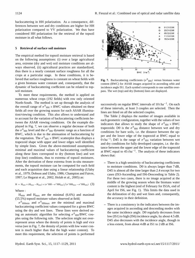
backscattering in HH polarization. As a consequence, dif-ferences between wet and dry conditions are higher for HHpolarization compared to VV polarization. We thus haveconsidered HH polarization for the retrieval of the topsoilmoisture in all what follows.

5 Retrieval of surface soil moisture

The empirical method for topsoil moisture retrieval is basedon the following assumptions: (i) over a large agriculturalarea, extreme (dry and wet) soil moisture conditions are al-ways observed, (ii) agricultural practices are standardized,thus there is a nearly constant surface roughness for all thecrops at a particular stage. In these conditions, it is be-lieved that surface roughness is constant on wheat fields witha given biomass water constant and, consequently, that thedynamic of backscattering coefficient can be related to top-soil moisture.

To meet these requirements, the method is applied onnumerous wheat crops (192 fields) with row only orientedNorth-South. The method is set up through the analysis ofthe overall range ofσ 0

HH ×BWC values obtained on thesefields all over the growing season for each ASAR illumina-tion/viewing condition. This also allows to understand andto account for the variation of backscattering coefficients be-tween the ASAR viewing conditions. On the example dis-played in Fig. 7, we can observe a regular decrease of boththeσ 0

HH level and theσ 0HH dynamic range as a function of

BWC, which is due to the attenuation of backscattering bythe vegetation. Theσ 0

HH × BWC scatterplot thus displays atrapezoid shape with upper and lower edges well identifiedby simple lines. Given the above-mentioned assumptions,minimal and maximal values of backscattering coefficientalong these lines correspond to dry (bottom line) and wet(top line) conditions, thus to extrema of topsoil moistures.After the derivation of these extrema from in-situ measure-ments, the topsoil moisture can be computed for each fieldand each acquisition date using a linear relationship (Ulabyet al., 1979; Dobson and Ulaby, 1986; Champion and Faivre,1997; Le Hegarat et al., 2002; Holah et al., 2005) as:

H = Hmin+(Hmax−Hmin)×(σ ◦HH−σ ◦HHmin)/(σ ◦HHmax−σ ◦HHmin) (3)

Where :Hmin and Hmax are the minimal (6.6%) and maximal

(55.5%) topsoil moisture values observed at field;σ 0

HHmin and σ 0HHmax are the minimal and maximal

backscattering coefficient values computed for a given BWCusing the dry and wet lines. These lines were derived us-ing an automatic algorithm for selectingσ 0

HH/BWC cou-ples using the following rule. The selection might not over-represent areas where the density of points is high and viceversa (see in Fig. 7, the density of points with low water con-tent is much higher than that the high water content). Tomeet this requirement, the selection of points is performed

Figure 7. Backscattering coefficients (0

HH) versus biomass water content (BWC) for ASAR images

acquired in ascending orbit and incidence angle IS1. Each symbol corresponds to one satellite

overpass. The wet (top) and dry (bottom) lines are displayed.

Fig. 7. Backscattering coefficients (σ0HH) versus biomass water

content (BWC) for ASAR images acquired in ascending orbit andincidence angle IS1. Each symbol corresponds to one satellite over-pass. The wet (top) and dry (bottom) lines are displayed.

successively on regular BWC intervals of 10 t ha−1. On eachof these intervals, at least 3 couples are selected. Then thelines are fitted on all the selected couples.

The Table 2 displays the number of images available ineach geometric configuration, together with the values of twoindicators that allows to study the shape ofσ 0

HH × BWCtrapezoids: D0 is theσ 0

HH distance between wet and dryconditions for bare soils, i.e. the distance between the up-per and the lower edge of the trapezoid at BWC equal to0 t ha−1; D45 is the range ofσ 0

HH variation between wetand dry conditions for fully developed canopies, i.e. the dis-tance between the upper and the lower edge of the trapezoidat BWC equal to 45 t ha−1. The analysis of these indicatorsshows that:

– There is a high sensitivity of backscattering coefficientsto moisture conditions. D0 is always larger than 7 dB,D45 is almost all the time larger than 2.4 except for twocases (IS3-Ascending and IS6-Descending in Table 2).For these two cases, there is no image acquired at themiddle of the growing season when the biomass watercontent is the highest (end of February for IS3A, end ofApril for IS6, see Fig. 1). This limits the data used inthe delineation of dry and wet lines and, consequently,the accuracy in their definition.

– There is a consistency in the indicators between the im-ages acquired in ascending and descending modes withthe same incidence angle. D0 regularly decreases fromlow (IS1) to high (IS6) incidence angle, by about 4.5 dB.D45 also decreases with the incidence angle, though ina less extent, from about 4 dB at IS1 to 2 dB at IS6.



Table 2. Number of images available for each ASAR viewing con-figuration, andσ0

HH distance between wet and dry conditions forbare soils (D0) and for fully developed canopies (D45).

Incidence Orbit pass Images used D0 D45

1 A 5 11.2 4.71 D 3 11.7 4.62 A 4 10.1 2.92 D 3 9.3 4.23 A 2 9.0 1.63 D 4 9.6 3.94 A 4 7.7 3.14 D 5 7.2 2.86 A 4 7.0 2.46 D 3 7.0 0.6

Figure 8. Estimated versus measured topsoil moisture. The different symbols correspond to three

successive wheat vegetative periods: (i) the beginning (‘+’) with biomass water content (BWC)

between 0 to 5 t ha-1

, (ii) the middle (‘o’) before senescence starts with BWC between 5 and 65 t.ha-

1, and the end (‘×’) associated to leaf senescence.

Fig. 8. Estimated versus measured topsoil moisture. The differ-ent symbols correspond to three successive wheat vegetative peri-ods: (i) the beginning (“+”) with biomass water content (BWC) be-tween 0 to 5 t ha−1, (ii) the middle (“o”) before senescence startswith BWC between 5 and 65 t ha−1, and the end (“×”) associatedto leaf senescence.

The retrieval of top soil moisture (Eq. 3) is independentlyapplied for each image using the dry and wet lines associatedwith a given acquisition geometry. The whole processing re-sults in estimates of topsoil moisture for 192 fields with roworiented North-South all over the study area at each satelliteoverpass.

Figure 9.0

HH to biomass water content scatterplot at the agricultural season beginning for fields

with North-South row orientations (ASAR image acquired the 01/01/2008, in ascending orbit, and

incidence angle 1).

Fig. 9. σ0HH to biomass water content scatterplot at the agricul-

tural season beginning for fields with North-South row orientations(ASAR image acquired the 01/01/2008, in ascending orbit, and in-cidence angle 1).

The retrieved values are compared to the topsoil moisturemeasured using TDR sensors. It should be kept in mind thatthese measurements are very local, whereas the values de-rived fromσ 0

HH correspond to 5 ha area. The result of thiscomparison is displayed in Fig. 8. The agreement betweenestimated and measured topsoil moisture is globally ratherpoor (R2 = 0.48, RMSE = 9.8%, 47% in relative value), buta deep analysis shows that it depends on the wheat growingphase:

– at the beginning of the agricultural season (“+” sym-bols in Fig. 8, BWC between 0 to 5 t ha−1), there isno relationship at all between estimates and measure-ments. In order to get a better understanding of thisscattering, we analysed the variation ofσ 0

HH as a func-tion of the biomass water content for the first acquisitiondate. At this time of year, BWC ranges between 0 and7 t ha−1, whereas the topsoil is rather dry since the firstirrigation is not operated. Topsoil moisture was around19% for the two fields equipped with TDR probes. Inthis case,σ 0

HH appears mainly sensitive to the biomasswater content, displaying a peak when BWC reaches3 t ha−1 (Fig. 9).

– at the end of the agricultural season (“×” symbols inFig. 8), the method also provides with poor results. Aprobable explanation is that estimates are attempted forfields in very different conditions: mature and senescentcanopies or dry plant litter after harvest.

– for the intermediate case, i.e. BWC between 5 and65 t ha−1 before senescence starts, (“o” symbols inFig. 8), the estimated topsoil moisture appears well cor-related with observation:R2 is around 0.64 and theRMSE is 8.8% (0.088 m3 m−3, 34% in relative value).



Figure 10.Time course of topsoil moisture (average and standard deviation) retrieved on field 5

together with the irrigation periods (vertical dotted gray lines) and precipitation (black line at the

bottom of the y-axis). The days are numbered from January 1st, 2007.

Fig. 10. Time course of topsoil moisture (average and standard de-viation) retrieved on field 5 together with the irrigation periods (ver-tical dotted gray lines) and precipitation (black line at the bottom ofthe y-axis). The days are numbered from 1 January 2007.

A deeper examination of these data did not allow tomake a distinction neither between the different acquisi-tion geometry nor between the different stages of vege-tation growing. This means that the inversion procedureworks even for high incidence angles and when the veg-etation is fully developed.

In order to evaluate the spatial and temporal variationsof topsoil moisture, the inversion procedure was applied onthe twelve fields where irrigation practices were recorded(see Fig. 1). According to the previous finding, the inver-sion algorithm was set up only when the biomass water con-tent exceeds 5 t ha−1 and in absence of plant senescence, i.e.when the air temperature accumulated from emergence is be-low the threshold defining the senescence temperature in theSAFY model.

The Table 3 shows the topsoil moisture derived fromASAR averaged on a 5-day period before and after the firstand the second irrigation times. In most of cases, the val-ues of topsoil moisture appear consistent with the irrigationschedules: topsoil moisture ranges from about 9 to 31% be-fore the irrigation times and from 20% to 50% after irrigationtimes; their averaged values are much lower before irrigationtimes (24% and 21% for the first and the second irrigation,respectively) than after (40% and 33% for the first and thesecond irrigation, respectively). This general trend is pre-served for 10 of the 12 fields analysed, except on : (i) field1, where the topsoil moisture is higher before than after thefirst irrigation time and the value before the second irriga-tion appear unrealistically low; (ii) field 3, where the top-soil appear dry both before and after the second irrigationtime. Additional data would be necessary to explain whythe method fails in these two cases, still the main possiblecauses are miss-collection of irrigation data (periods and/oramounts) and local variations of the soil properties (texture,roughness).

Figure 11.Topsoil moisture (TSM) mapped over the different geographical units (about 5 ha) of the

field 5 (see Table 3 and Fig.1). The 12 first dates, corresponding to those shown on Fig. 10, are

presented together with the incidence angle of the based Envisat acquisition.

TSM [%]

Fig. 11. Topsoil moisture (TSM) mapped over the different geo-graphical units (about 5 ha) of the field 5 (see Table 3 and Fig. 1).The 12 first dates, corresponding to those shown on Fig. 10, arepresented together with the incidence angle of the based Envisatacquisition.

Finally, a detailed analysis of the temporal and spatial vari-ations of topsoil moisture is presented for field 5 as a rep-resentative case (Figs. 10 and 11). On this field, the timecourse of the mean topsoil moisture appears coherent withthe irrigation schedules all over the season: the topsoil mois-ture sharply rises during irrigation times then continuouslydecreases after irrigation times (Fig. 10). Figure 11 displaysthe spatial variations of the topsoil moisture derived over the8 segments within the field 5 from the 12 ASAR images suc-cessively acquired around the first irrigation time. Beforeirrigation, the topsoil moisture appears homogeneous with aslight decrease from the first image (30/01/2008) to the third(05/02/2008). The watercourse can be easily identified fromthe images acquired at the time of irrigation (08/02/2008to 21/02/2008): the topsoil moisture suddenly increases onseveral segments (blue to red colors in Fig. 11), firstly onthe eastern part of the field (08/02/2008 and 11/02/2008),then on the middle (14/02/2008) and on the western parts(15/02/2008 and 21/02/2008). After irrigation (21/02/2008to 08/03/2008), the topsoil moisture continuously decreasesand the impact of irrigation on its spatial distribution issmoothed with time. All this is also visible when lookingat the standard deviation of the mean topsoil moisture cal-culated over the 8 segments included in field 5 (Fig. 10).The standard deviation is minimal before and a long timeafter the first irrigation time when the soil is homogeneouslydry; it is maximal at the middle of irrigation times when seg-ments may not been irrigated yet, under irrigation or alreadyirrigated.



Table 3. Topsoil moisture derived from ASAR image before and after the first and the second irrigations on the twelve fields where irrigationschedules were collected during the experiment.

Fields Area (ha)Before Irrigation 1 After Irrigation 1 Before Irrigation 2 After Irrigation 2

Nb Image Mean Nb Image Mean Nb Image Mean Nb Image Mean

1 32.8 2 29.1 3 27.7 2 8.6 2 23.72 45.1 0 x 2 46.2 2 29.1 0 x3 22.8 0 x 1 33.2 3 16.5 2 19.84 47.8 2 31.5 2 44.7 2 19.2 2 39.15 48.1 2 21.9 1 39.7 3 23.7 1 35.56 47.1 0 x 3 44.5 2 28.6 2 35.27 19.7 1 29.1 2 42.3 1 18.9 1 35.98 19.1 2 20.9 1 46.6 3 12.6 2 21.09 19.0 0 x 0 x 1 21.4 2 45.710 19.2 2 16.6 1 49.3 2 12.9 1 40.011 76.3 1 20.0 2 31.6 2 28.0 1 36.512 94.0 2 24.1 2 38.6 1 27.9 0 x

6 Conclusion

The potentialities of ASAR data for the monitoring of soilmoisture conditions in agricultural lands were investigatedfor wheat crops monitored through the SAFY vegetationfunctioning model and time series of Formosat-2 images.The normalized difference vegetation index derived fromFormosat-2 data was linked to the green leaf area index(GLA) with an accuracy of about 25%. GLA is a key variablefor the parametrization of photosynthesis, which was incor-porated into the SAFY model to provide spatial estimates ofbiomass water content (BWC) over up to 200 wheat fields.The value of Formosat-2 data acquired with both a high spa-tial resolution and a frequent revisit for the monitoring ofcrop growth should be firstly underlined. It allows increas-ing the number of data available to get a better understandingof radar signal over irrigated wheat fields.

Despite the homogeneity of agricultural practices and ofwheat canopies in the Yaqui area, the joint analysis of radarbackscattering (σ 0

HH) and BWC shows the complexity ofthe radar response for agricultural lands, due to a highvariability of both surface roughness and topsoil moisture.The sensitivity of the backscattering coefficient to topsoilmoisture is highlighted for a large field for which spatialtrends and discontinuities ofσ 0

HH were observed in con-sistency with soil watering during irrigation times and soildrying out of irrigation times. This sensitivity was observedwhatever the acquisition angle and whatever the recoveringof soil by vegetation, even when BWC was very high. Thisapproach appears suitable to detect on-going irrigated areasall over the wheat growing season.

This previous findings allow to set up an empirical methodfor the retrieval of topsoil moisture from the combination ofASAR images and spatial estimates of BWC. The method is

original since it is based on the spatial variation ofσ 0HH over

a large area rather than on its temporal variation over a par-ticular area. The method allows the retrieval of topsoil mois-ture from its minimal to its maximal value (6%–56%) withan error about 9% (0.09 m3 m−3, 35% in relative value) for along period between wheat tillering and senescence phases.These performances appear significant since estimates areperformed at the key time of crop growth and under a largerange of biomass water content (from 5 to 65 t ha−1) with allASAR images available (whatever the incidence angles from15 to 40◦).

The method provides estimates of topsoil moisture at afield resolution (∼5 ha) without an exact knowledge on sur-face roughness. An additional advantage is that it not re-quired to normalise satellite observations at a same incidenceangle, which is not trivial on surfaces that experiences quickvariations such as wheat fields. All these points make themethod very attractive for operational application over largeareas. However, the method requires the availability of nu-merous images both in the solar and the micro-wave domainof the electromagnetic spectrum. Furthermore, it was as-sumed that the surface roughness is stable at a given growingphase (same biomass water content). This assumption is ver-ified in the case of the Yaqui area where large fields are flat-tened and cropped with modern and mechanized agriculturalpractices. Application to other areas where these conditionsare not met would require adaptation, especially if the regionis not rather homogeneous in terms of agricultural practices.

Acknowledgements.The Yaqui 2007–2008 experiment was orga-nized jointly by the IRD-CESBIO, ITSON, UNISON and COLPOSinstitutions with fundings of the European Union (7th PCRD,PLEIADeS program,http://www.pleiades.es/), the French INSU-PNTS (“Programme National de Teledetection Spatiale”) andCNES-TOSCA (“Terre Ocean Surface Continentale Atmosphere”)


http://www.pleiades.es/


programs and the Mexican CONACYT program. We are indebtedto ESA for the programming and the delivery of ASAR images aswell as to NSPO, SPOT-Image, and CNES for the programming,the delivery and the processing of Formosat-2 images.

Edited by: D. F. Prieto

The publication of this article is financed by CNRS-INSU.

References

Asrar, G., Fuchs, M., Manemasu, E. T., and Hatfield, J. L.: Estimat-ing absorbed photosynthetic radiation and leaf area index fromspectral reflectance in wheat, Agron. J., 76, 300–306, 1984.

Baret, F. and Guyot, G.: Potentials and limits of vegetation indicesfor LAI and APAR assessment, Remote Sens. Environ., 35, 161–173, 1991.

Bastiaanssen, W. G. M., Molden, D. J., and Makin, I. W.: Remotesensing for irrigated agriculture: examples from research andpossible applications, Agr. Water Manage., 46, 137–155, 2000.

Beaudoin, A., Le Toan, T., and Gwyn, Q. H. J.: SAR observa-tions and modeling of the C-band backscatter variability due tomultiscale geometry and soil moisture, IEEE T. Geosci. Remote,28(5), 886–895, 1990.

Boote, K. J., Jones, J. W., and Pickering, N. B.: Potential uses andlimitations of crop models, Agron. J., 88, 704–716, 1996.

Bracaglia, M., Ferrazzoli, P., and Guerriero, L.: A fully polarimetricmultiple scattering model for crops, Remote Sens. Environ., 54,170–179, 1995.

Brown, S. C. M., Quegan, S., Morrison, K., Bennett, J. C., andCookmartin, G.: High-Resolution Measurements of Scatteringin Wheat Canopies-Implications for Crop Parameter Retrieval,IEEE T. Geosci. Remote, 41(7), 1602–1610, 2003.

Bsaibes, A., Courault, D., Baret, F., Weiss, M., Olioso, A., Ja-cob, F., Hagolle, O., Marloie, O., Bertrand, N., Desfond, V., andKzemipour, F.: Albedo and LAI estimates from FORMOSAT-2data for crop monitoring, Remote Sens. Environ., 113, 716–729,2009.

Carlson, T. N. and Ripley, D. A.: On the relation between NDVI,vegetation cover and leaf area index, Remote Sens. Environ., 62,241–252, 1997.

Champion, I. and Faivre, R.: Sensitivity of the radar signal to soilmoisture: variation with incidence angle, frequency and polar-ization, IEEE T. Geosci. Remote, 35, 781–783, 1997.

Chern, J.-S., Ling, J., and Weng, S.-L.: Taiwan’s second remotesensing satellite, Acta Astronaut., 63, 1305–1311, 2008.

Claverie, M., Demarez, V., Duchemin, B., Maire, F., Hagolle, O.,Keravec, P., Marciel, B., Ceschia, E., Dejoux, J.-F., and Dedieu,G.: Spatialisation of crop Leaf Area Index and Biomass by com-bining a simple crop model and high spatial and temporal resolu-

tions remote sensing data, Int. Geosci. Remote Se., Cape Town,South Africa, 2009.

Dente, L., Satalino, G., Mattia, F., and Rinaldi, M.: Assimilationof leaf area index derived from ASAR and MERIS data intoCERES-Wheat model to map wheat yield, Remote Sens. Envi-ron., 112, 1395–1407, 2008.

Dobson, M. C. and Ulaby, F. W.: Active microwave soil moistureresearch. IEEE T. Geosci. Remote, 24, 23–6, 1986.

Duchemin, B., Hadria, R., Er-Raki, S., Boulet, G., Maisongrande,P., Chehbouni, A., Escadafal, R., Ezzahar, J., Hoedjes, J., Khar-rou, M. H., Khabba, S., Mougenot, B., Olioso, A., Rodriguez,J.-C., and Simonneaux, V.: Monitoring wheat phenology andirrigation in Center of Morocco: on the use of relationship be-tween evapotranspiration, crops coefficients, leaf area index andremotely-sensed vegetation indices, Agr. Water Manage., 79, 1–27, 2006.

Duchemin, B., Hagolle, O., Mougenot, B., Benhadj, I., Hadria, R.,Simonneaux, V., Ezzahar, J., Hoedjes, J., Khabba, S., Kharrou,M. H., Boulet, G., Dedieu, G., Er-Raki, S., Escadafal, R., Olioso,A., and Chehbouni, A. G.: Agrometerological study of semi-aridareas: an experiment for analysing the potential of FORMOSAT-2 time series of images in the Tensift-Marrakech plain, Int. J.Remote Sens., 29, 5291–5300, 2008a.

Duchemin, B., Maisongrande, P., Boulet, G., and Benhadj, I.: Asimple algorithm for yield estimates: calibration and evalua-tion for semi-arid irrigated winter wheat monitored with ground-based remotely-sensed data, Environ. Modell. Softw., 23, 876–892, 2008b.

Duchemin, B., Fieuzal, R., Augustin Rivera, M., Boulet, G., Er-Raki, S., Ezzahar, J., Mougenot, B., Perez-Ruiz, E. R., Ro-driguez, J. C., Hagolle, O., Garatuza-Payan, J., Watts, C., Es-cadafal, R., and Chehbouni, A.: Impact of sowing date on yieldand water-use-efficiency of wheat analyzed through spatial mod-eling and FORMOSAT-2 images, submitted to Remote Sens. En-viron., 2010.

ESA: GMES Sentinel-2 mission requirement document, No. EOP-SM/1163/MR-dr v2.0,http://esamultimedia.esa.int/docs/GMES/Sentinel-2MRD.pdf, (2007).

Faivre, R., Leenhardt, D., Voltz, M., Benoit, M., Papy, F., Dedieu,G., and Wallach, D.: Spatialising crop models, Agronomie, 24,205–217, 2004.

Garrigues, S., Allard, D., Baret, F., and Weiss, M.: Quantifying spa-tial heterogeneity at the landscape scale using variogram models,Remote Sens. Environ., 103, 81–96, 2006.

Hadria, R., Duchemin, B., Jarlan, L., Dedieu, G., Baup, F., Khabba,S., Olioso, A., and Le Toan, T.: Potentiality of optical and radarsatellite data at high spatio-temporal resolutions for the monitor-ing of irrigated wheat crops in Morocco, Int. J. Appl. Earth Obs.,12, S32–S37, 2010.

Hagolle, O., Dedieu, G., Mougenot, B., Debaecker, V., Duchemin,B., and Meygret, A.: Correction of aerosol effects on multi-temporal images acquired with constant viewing angles: applica-tion to Formosat-2 images, Remote Sens. Environ., 112, 1689–1701, 2008.

Holah, H., Baghdadi, N., Zribi, M., Bruand, A., and King C.: Poten-tial of ASAR/ENVISAT for the characterization of soil surfaceparameters over bare agricultural fields, Remote Sens. Environ.,96(1), 78–86, 2005.

Jarlan, L., Mougin, E., Frison, P. L., Mazzega, P., and Hiernaux,


http://esamultimedia.esa.int/docs/GMES/Sentinel-2_MRD.pdf

http://esamultimedia.esa.int/docs/GMES/Sentinel-2_MRD.pdf


P.: Analysis of ERS wind scatterometer time series over Sahel(Mali), Remote Sens. Environ., 81, 404–415, 2002.

Le Hegarat-Mascle, S., Zribi, M., Alem, F., and Weisse, A.: Soilmoisture estimation from ERS/SAR data: Toward an opera-tional methodology, IEEE T. Geosci. Remote, 40(12), 2647–2658, 2002.

Lobell, D. B., Ortiz-Monasterio, J. I, Asner, G. P., Matson, P. A,Naylor, R. L., and Falcon, W. P.: Analysis of wheat yield andclimatic trends in Mexico, Field Crop. Res., 94, 250–256, 2005.

Maas, S. J.: Parameterized model of gramineous crop growth, 1.Leaf-area and dry mass simulation, Agron. J., 85, 348–353,1993.

Mattia, F., Le Toan, T., Picard, G., Posa, F. I., D’Alessio, A., Notar-nicola, C., Gatti, A. M., Rinaldi, M., Satalino, G., and Pasquar-iello, G.: Multitemporal C-Band Radar Measurements on WheatFields, IEEE T. Geosci. Remote, 41(7), 1551–1560, 2003.

Monteith, J. L. and Moss, C. J.: Climate and the Efficiency ofCrop Production in Britain, Philos. T. Roy. Soc. B, 281, 277–294, 1977.

Moran, M. S., Hymer, D. C., Qi, J., and Kerr, Y.: Comparison ofERS-2 SAR and Landsat TM imagery for monitoring agriculturalcrop and soil conditions, Remote Sens. Environ., 79, 243–252,2002.

Moulin, S., Bondeau, A., and Delecolle, R.: Combining agricul-tural crop models and satellite observations from field to regionalscales, Int. J. Remote Sens., 19, 1021–1036, 1998.

Ortiz-Monasterio, J. I. and Lobell, D. B.: Remote sensing assess-ment of regional yield losses due to sub-optimal planting datesand fallow period weed management, Field Crop. Res., 101, 80–87, 2007.

Picard, G., Le Toan, T., and Mattia, F.: Understanding C-band radarbackscatter from wheat canopy using a multiple-scattering co-herent model, IEEE T. Geosci. Remote Sens., 41(7), 1583–1591,2003.

Rahman, H. and Dedieu, G.: SMAC: a simplified method for the at-mospheric correction of satellite measurements in the solar spec-trum, Int. J. Remote Sens., 15.1, 123–143, 1994.

Rodriguez, J.-C., Duchemin, B., Hadria, R., Watts, C., Garatuza,J., Chehbouni, A., Khabba, S., Boulet, G., Palacios, R., andLahrouni, A.: Wheat yield estimation using remote sensingand the STICS model in the semiarid valley of Yaqui, Mexico,Agronomie, 24, 295–304, 2004.

Satalino, G., Mattia, F., Davidson, M., Le Toan, T., Pasquarello, G.,and Borgeaud, M.: On current limits of Soil Moisture Retrievalfrom ERS SAR data, IEEE T. Geosci. Remote Sens., 40, 2438–2447, 2003.

Torres, R., Buck, C., Guijarro, J., Suchail, J. L., and Schonenberg,A.: The ENVISAT ASAR Instrument Verification and Character-isation, ESA CEOS SAR Workshop, ESA-SP450, October 1999.

Ulaby, F. T., Bradley, G. A., and Dobson, M. C.: Microwavebackscatter dependence on surface roughness in soil moistureand soil texture: Part II-Vegetation-covered soil, IEEE T. Geosci.Remote Sens., 17, 33–40, 1979.

Ulaby, F. T., Fung, A. K., and Moore, R. K.: Microwave and remotesensing active and passive (Norwood, MA: Artech House), 1986.

Weiss, M., Baret, F., Smith, G. J., Jonckheere, I., and Coppin, P.:Review of methods for in situ leaf area index (LAI) determina-tion: Part II. Estimation of LAI, errors and sampling, Agr. ForestMeteorol., 121, 37–53, 2004.

Zribi, M., Le Hegarat-Mascle, S., Ottle, C., Kammoun, B., andGuerin, C.: Surface soil moisture estimation from the synergis-tic use of the (multi-incidence and multi-resolution) active mi-crowave ERS Wind Scatterometer and SAR data, Remote Sens.Environ., 86, 30–41, 2003.


combined use of optical and radar satellite data for the

Documents