combining hyperspectral uav and mul
TRANSCRIPT
LUMA-GIS Thesis nr 32
Caroline Gevaert
2014
Department of
Physical Geography and Ecosystem Science
Centre for Geographical Information Systems
Lund University Sölvegatan 12
S-223 62 Lund
Sweden
COMBINING HYPERSPECTRAL UAV AND
MULTISPECTRAL FORMOSAT-2 IMAGERY
FOR PRECISION AGRICULTURE
APPLICATIONS

ii
Caroline Gevaert (2014). Combining Hyperspectral UAV and Multispectral Formosat-2 Imagery
for Precision Agriculture Applications.
Master degree thesis, 30/ credits in Master in Geographical Information Sciences
Department of Physical Geography and Ecosystems Science, Lund University

iii
Combining Hyperspectral UAV and Multispectral Formosat-2 Imagery for Precision Agriculture
Applications
Caroline Gevaert
Master thesis, 30 credits, in Geographical Information
Sciences
Supervisor:
Jing Tang
Department of Physical Geography and Ecosystem Sciences
Lund University

iv
v
Abstract In the context of threatened global food security, precision agriculture provides a solution which can
maximize yield to meet the increased demands of food while minimizing both economic and
environmental costs of food production. Detailed information regarding crop status is crucial for precision
agriculture. Remote sensing provides an efficient way to obtain crop biophysical status information, such
as canopy nitrogen content, leaf coverage, and plant biomass. However, individual sensors do not
normally meet both spatial and temporal requirements for precision agriculture. Therefore, this study
investigates different fusion methods which can be used to combine imagery from various sensors to
overcome the limitations of each individual sensor. The imagery utilized in the current study consists of
multispectral satellite (Formosat-2) and hyperspectral Unmanned Aerial Vehicle (UAV) imagery of a
potato field in the Netherlands.
The imagery from both platforms was combined in two ways. Firstly, data fusion methods brought the
spatial resolution of the Formosat-2 imagery (8 m) down to the spatial resolution of the UAV imagery (1
m). Two data fusion methods were applied: an unmixing-based algorithm and the Spatial and Temporal
Adaptive Reflectance Fusion Model (STARFM). The unmixing-based method produced vegetation
indices which were highly correlated to the measured LAI (rs= 0.866) and canopy chlorophyll values
(rs=0.884), whereas the STARFM showed lower correlations (rs=0.477 and rs=0.431, respectively).
Secondly, a Spectral-Temporal Reflectance Surface (STRS) was constructed to interpolate daily 101-band
reflectance spectra using both sources of imagery. The STRS were interpolated using a new method,
which utilizes Bayesian theory to obtain realistic spectra and accounts for sensor uncertainties. The
resulting surface obtained a high correlation to LAI (rs=0.858) and canopy chlorophyll (rs=0.788)
measurements at field level.
The usefulness of these multi-sensor datasets was further analyzed regarding their ability to map crop
status variability and predict yield. The results showed the capability of the multi-sensor datasets to
characterize significant differences of crop status due to differing nitrogen fertilization regimes from June
to August. Meanwhile, the yield prediction models based purely on the vegetation indices extracted from
the unmixing-based fusion dataset explained 52.7% of the yield variation, which is lower than that
explained by the STRS (72.9%). Around 75.3% of the yield can be explained by a regression model using
direct field LAI and chlorophyll measurements.
The results of the current study indicate that the limitations of each individual sensor can be largely
surpassed by combining multiple sources of imagery. This can be very beneficial for precision agriculture
management decisions, which require require reliable and high-quality information. Further research
could focus on the integration of data fusion and STRS techniques, and the inclusion of imagery from
additional sensors.
vi
Samenvatting
In een wereld waar toekomstige voedselzekerheid bedreigd wordt, biedt precisielandbouw een oplossing
die de oogst kan maximaliseren terwijl de economische en ecologische kosten van voedselproductie
beperkt worden. Om dit te kunnen doen is gedetailleerde informatie over de staat van het gewas nodig.
Remote sensing is een manier om biofysische informatie, waaronder stikstof gehaltes en biomassa, te
verkrijgen. De informatie van een individuele sensor is echter vaak niet genoeg om aan de hoge eisen
betreft ruimtelijke en temporele resolutie te voldoen. Deze studie combineert daarom de informatie
afkomstig van verschillende sensoren, namelijk multispectrale satelliet beelden (Formosat-2) en
hyperspectral Unmanned Aerial Vehicle (UAV) beelden van een aardappel veld, in een poging om aan de
hoge informatie eisen van precisielandbouw te voldoen.
Ten eerste werd gebruik gemaakt van datafusie om de acht Formosat-2 beelden met een resolutie van 8 m
te combineren met de vier UAV beelden met een resolutie van 1 m. De resulterende dataset bestaat uit
acht beelden met een resolutie van 1 m. Twee methodes werden toegepast, de zogenaamde STARFM
methode en een unmixing-based methode. De unmixing-based methode produceerde beelden met een
hoge correlatie op de Leaf Area Index (LAI) (rs= 0.866) en chlorofyl gehalte (rs=0.884) gemeten op
veldnieveau. De STARFM methode presteerde slechter, met correlaties van respectievelijk rs=0.477 en
rs=0.431. Ten tweede werden Spectral-Temporal Reflectance Surfaces (STRSs) ontwikkeld die een
dagelijks spectrum weergeven met 101 spectrale banden. Om dit te doen is een nieuwe STRS methode
gebaseerd op de Bayesiaanse theorie ontwikkeld. Deze produceert realistische spectra met een
overeenkomstige onzekerheid. Deze STRSs vertoonden hoge correlaties met de LAI (rs=0.858) en het
chlorofyl gehalte (rs=0.788) gemeten op veldnieveau.
De bruikbaarheid van deze twee soorten datasets werd geanalyseerd door middel van de berekening van
een aantal vegetatie-indexen. De resultaten tonen dat de multi-sensor datasets capabel zijn om significante
verschillen in de groei van gewassen vast te stellen tijdens het groeiseizoen zelf. Bovendien werden
regressiemodellen toegepast om de bruikbaarheid van de datasets voor oogst voorspellingen. De
unmixing-based datafusie verklaarde 52.7% van de variatie in oogst, terwijl de STRS 72.9% van de
variabiliteit verklaarden.
De resultaten van het huidige onderzoek tonen aan dat de beperkingen van een individuele sensor
grotendeels overtroffen kunnen worden door het gebruik van meerdere sensoren. Het combineren van
verschillende sensoren, of het nu Formosat-2 en UAV beelden zijn of andere ruimtelijke
informatiebronnen, kan de hoge informatie eisen van de precisielandbouw tegemoet komen.

vii
Acknowledgements
The current research would not have been possible without the help of many people. Firstly, Dr. Lammert
Kooistra from the WU-GRS, who served as an external supervisor for this thesis. Thank you for
providing me with the opportunity to work on this subject and for all your helpful comments and
guidance. Many thanks also to Dr. Juha Suomalainen from the WU-GRS who developed the UAV system
and processed the imagery, and to Dr. Javier García-Haro from the University of Valencia who played a
significant role in developing the unmixing-based fusion method used in this paper.
I would also like to thank my supervisor at Lund University, Jing Tang for her help in the development of
this thesis. And to all the team behind the LUMA-GIS program, who I have not (yet) been able to thank
face-to-face, but who have put together a wonderful Master’s program. This provides a unique
opportunity for many students throughout the world, and I personally am very happy that I was able to
participate.
The help of Dr. Cheng-Chien Liu of National ChengKung University is acknowledged for kindly
providing the Formosat-2 spectral response data.
Finally, I would also like to take this opportunity to thank my family. For their patience and support.
viii
Table of Contents
Introduction ........................................................................................................................................................... 1
Objectives ............................................................................................................................................................. 4
Background ........................................................................................................................................................... 5
3.1 Data fusion ................................................................................................................................................... 5
3.2 Spectral-Temporal Reflectance Surfaces (STRS) ........................................................................................ 5
3.3 Vegetation indices ........................................................................................................................................ 6
3.4 Yield prediction ............................................................................................................................................ 7
Data and Methodology .......................................................................................................................................... 9
4.1 Study area ..................................................................................................................................................... 9
4.2 Data ............................................................................................................................................................ 11
4.2.1 Formosat-2 imagery .......................................................................................................................... 11
4.2.2 UAV imagery .................................................................................................................................... 12
4.2.3 Field data ........................................................................................................................................... 12
4.3 Methods ...................................................................................................................................................... 13
4.3.1 Data pre-processing ........................................................................................................................... 14
4.3.2 Data Fusion ....................................................................................................................................... 16
4.3.3 STRS ................................................................................................................................................. 16
4.3.4 Vegetation indices ............................................................................................................................. 20
4.3.5 Statistical analyses ............................................................................................................................. 20
Results ................................................................................................................................................................. 22
5.1 Data pre-processing .................................................................................................................................... 22
5.1.1 Formosat-2 imagery .......................................................................................................................... 22
5.1.2 Yield interpolation ............................................................................................................................. 22
5.2 Data fusion ................................................................................................................................................. 23
5.3 STRS .......................................................................................................................................................... 26
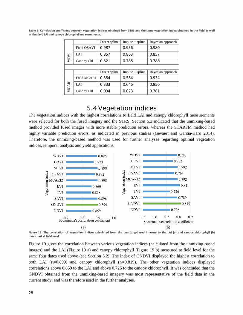
5.4 Vegetation indices ...................................................................................................................................... 28
5.5 Statistical analysis ...................................................................................................................................... 29
5.5.1 Variation detection during the growing season ................................................................................. 29
5.5.2 Yield prediction ................................................................................................................................. 31
Discussion ........................................................................................................................................................... 35
6.1 Combination of multi-sensor imagery ........................................................................................................ 35
6.2 Vegetation indices ...................................................................................................................................... 36
6.3 Fused datasets for in-season crop status analysis and yield prediction .................................................... 36
6.4 Yield prediction .......................................................................................................................................... 37
Conclusions ......................................................................................................................................................... 38
References ........................................................................................................................................................... 39
Series from Lund University ............................................................................................................................... 44
Appendix 1: Atmospheric correction of Formosat-2 imagery .................................................................................. 1
Appendix 2: Data fusion parameter optimization .................................................................................................... 1
Appendix 3: Vegetation indices ............................................................................................................................... 1
Appendix 4: WHISPERS 2014 Submission ............................................................................................................. 1
1
Introduction Global food security is threatened by increased demands from a growing global population, increased
competition for land, and the need for sustainable production with lower environmental externalities
(Godfray et al. 2010). Precision agriculture is often flagged as a key “sustainable intensification” method,
as it aims to maximize the agricultural production in a sustainable manner (The Royal Society 2009). One
of the key steps is to quantify both spatial and temporal variations of crop conditions and apply various
management strategies within a field according to these differences (Gebbers and Adamchuk 2010). By
applying the exact amount of input resources where and when it is needed, the yield can be maximized
while reducing the application of fertilizer and pesticides - which is economically beneficial for the
farmer and environmentally beneficial for the general population (Gebbers and Adamchuk 2010; Clay
and Shanahan 2011).
Remote sensing is capable of identifying variation in biophysical parameters such as canopy nitrogen
content and plant biomass (Clevers and Kooistra 2012). It plays a key role in agricultural monitoring
(Jones and Vaughan 2010), especially in the identification of nitrogen stress (Mcmurtrey et al. 2003;
Goffart et al. 2008; Diacono et al. 2012). It is recognized as one of the key methods to quantify both
temporal and spatial variations of crop conditions which are essential for the application of precision
agriculture (Gebbers and Adamchuk 2010). Yield-prediction models are often based on the assumption
that yield production is influenced by measureable biophysical parameters such as LAI and chlorophyll,
variations in which can be identified in remotely-sensed images through the use of vegetation indices
(Bala and Islam 2009; Shillito et al. 2009; Gontia and Tiwari 2011; Neale and Sivarajan 2011; Rembold
et al. 2013; Ramírez et al. 2014). Yield prediction based on remotely sensed biophysical parameters is
more challenging in the current situation, as potato tubers are grown below-ground (Ramírez et al. 2014).
Optical remote sensing imagery can be divided into multispectral satellite imagery and hyperspectral
imagery. Multispectral imagery consists of a limited number of broad spectral bands (Christophe et al.
2005), and contains general information regarding vegetation structure and crop greenness (Zarco-Tejada
et al. 2005). Hyperspectral imagery contains more than 100 spectral bands, which are also much narrower
than multispectral imagery and provide a continuous reflectance spectrum (Christophe et al. 2005). Such
imagery is capable of providing more detailed information and specific crop physiological parameters,
such as chlorophyll, carotenoids, and water conditions (Zarco-Tejada et al. 2005). Multispectral imagery
has been available longer and is more widespread, however the increased precision of hyperspectral
imagery for vegetation monitoring is increasingly being recognized in the international community
(Haboudane et al. 2004).
Many studies describe the use of multispectral satellite imagery for precision agriculture applications
(Plant 2001; Cohen et al. 2010; Lee et al. 2010; Lunetta et al. 2010; Ge et al. 2011; Diacono et al. 2012).
However, factors such as inadequate spatial or temporal resolution (Merlin et al. 2010) and cloud cover
(Mulla 2013) have limited the effectiveness of utilizing such satellite imagery (Dorigo et al. 2007).
Alternatively, Unmanned Aerial Vehicles (UAV) have been proposed for precision agriculture
applications (Berni et al. 2009; Kooistra et al. 2012; Zhang and Kovacs 2012; Kooistra et al. 2013) as
they can provide imagery with a higher spatial resolution and more flexible acquisition times compared to
2
satellite imagery (Zhang and Kovacs 2012). Furthermore, UAVs fly under the clouds allowing them to
obtain imagery on cloudy days, which is a great benefit in areas with frequent cloud cover, such as the
Netherlands1. However, operational requirements may inhibit monitoring of large areas and the frequency
of flights (Zhang and Kovacs 2012). The current research investigates the integration of reflectance
information from multispectral satellite imagery and hyperspectral UAV imagery in two ways: (1) data
fusion to compare sensors of differing spatial resolution and (2) the creation of Spectral-Temporal
Reflectance Surfaces (STRS) to integrate the spectral and temporal resolutions of multiple sensors.
A potato field near Reusel, the Netherlands was selected for the study area (Kooistra et al. 2013). Four
dates of UAV images were obtained over the study area during the growing season of 2013. Formosat-2
satellite imagery is available over the zone at eight dates in the same growing season. Moreover, an
experimental set-up divided the field into four zones which were treated with four different nitrogen
application rates at the beginning of the growing season. During the entire growing season, weekly field
measurements of leaf chlorophyll, Leaf Area Index (LAI), and spectral reflectance were obtained for a
number of experimental plots. This creates a unique experimental set-up to analyze synergistic methods to
combine UAV and Formosat-2 imagery, and further enable us to evaluate the results using field data.
Data fusion is a possible method to combine imagery from sensors with differing spatial resolutions (Pohl
and Van Genderen 1998). Recently, many researchers have investigated the application of data fusion
between medium spatial-resolution imagery such as MODIS (Gao et al. 2006) and MERIS (Zurita-Milla
et al. 2008; Amorós-López et al. 2013) and high spatial-resolution datasets such as Landsat to obtain a
fused image dataset with a daily temporal resolution and a spatial resolution of 30 m. Two prevalent data
fusion methods are the Spatial and Temporal Adaptive Reflectance Fusion Model (STARFM) (Gao et al.
2006) and unmixing-based data fusion (Zurita-Milla et al. 2008; Amorós-López et al. 2013).
STARFM is the most widely-used data fusion algorithm for Landsat and MODIS imagery (Emelyanova
et al. 2013). It is one of the few data fusion methods which obtains surface reflectance calibrated to the
high-resolution image (Singh 2011). The method is particularly useful for detecting gradual changes over
large land areas, such as phenology studies (Gao et al. 2006; Hilker et al. 2009). Disadvantages of the
STARFM method include the requirement of a base pair of high- and medium-resolution images for
reference, dependency on the availability of homogenous medium-resolution pixels (Zhu et al. 2010), and
sensitivity to temporal variation of land cover (Gevaert and García-Haro 2014).
On the other hand, unmixing-based data fusion methods do not require corresponding spectral bands. It
therefore allows for the downscaling of additional spectral bands of the medium-resolution sensor (Zurita-
Milla et al. 2011; Amorós-López et al. 2013) and do not require a base image pair. The unmixing-based
method is less sensitive to temporal variations, and provides more stable errors (Gevaert and García-Haro
2014). An important difference with the STARFM method is that the unmixing-based method retains the
spectral information of the medium-resolution image, and thus does not provide reflectance calibrated to
1 During the growing season of 2013, the meteorological station nearest to the study area (Eindhoven) reported
79.1% of the days were at least half-clouded, and 57.8% of the days were heavily clouded (KNMI 2014).
3
the high-resolution image (Zurita-Milla et al. 2011; Amorós-López et al. 2013). A more detailed analysis
comparing various data fusion methods can be found in Gevaert (2013).
The current thesis hypothesizes that these two data fusion methods are also suitable for combining
multispectral Formosat-2 satellite imagery with hyperspectral UAV imagery. The fused dataset could
benefit from the spatial resolution of the UAV imagery (1 m), and the added temporal frequency of the
Formosat-2 imagery.
However the fused datasets obtained through both methods contain only four spectral bands, and do not
benefit from the additional spectral information contained in the UAV imagery. STRS are 4-dimensional
image datasets (row, line, wavelength, time) which illustrate how the spectrum of a certain pixel changes
over time. Previous studies have applied STRS to Landsat-5/TM and Landsat-7/ETM+ imagery to
characterize sugarcane harvests in Brazil (Mello et al. 2013), and to MERIS and MODIS imagery to
create a cloud-free image time series (Villa et al. 2013). A STRS is formed by interpolating the
reflectance of each pixel along the wavelength and temporal dimensions. Mello et al. (2013) utilized the
Polynomial Trend Surface (PTS) and Collocation Surface (CS) methods to interpolate the spectral and
temporal dimensions directly. Villa et al. (2013) first interpolated MERIS and MODIS spectra along the
wavelength dimension using a spline interpolation, and then interpolated along the temporal dimension
separately.
However, these STRS implementation methods have a number of limitations. Firstly, they do not account
for the physical characteristics of reflectance spectra. Therefore, the interpolated spectra may be
unrealistic, such as a missing red-edge for vegetation spectra (Figure 7 in Mello et al. 2013; Figure 1 in
Villa et al. 2013). Secondly, all imagery observations are weighted equally – the uncertainty of each
image is not taken into account. This thesis utilizes a new methodology to obtain STRS based on
Bayesian theory which could these limitations (Mello et al. 2013; Villa et al. 2013).
In sum, the purpose of this study is to investigate methods to combine multiple sources of imagery to
obtain a product which provides reliable information regarding crop status for precision agriculture
applications. Data fusion methods are applied to combine the spatial and spectral information from
satellite and UAV data. STRS methods are applied to combine the spectral and temporal information from
the multispectral and hyperspectral imagery. Finally, the ability of these methods to document variations
in crop biophysical parameters during the growing season and to explain yield variability are analyzed
through statistical methods.
4
Objectives The objective of the current research is to develop methods to combine the high temporal resolution of
multispectral Formosat-2 imagery and the high spatial and spectral resolution of hyperspectral UAV
imagery for precision agriculture applications.
This objective was achieved by completing the following steps:
Exploring a systematic scheme of combining multispectral and hyperspectral imagery for
precision agriculture.
Applying current data fusion methods for MODIS/MERIS and Landsat fusion to UAV and
Formosat-2 imagery.
Exploring the use of STRS to take advantage of the hyperspectral information of the UAV
imagery, and to provide daily reflectance data at plot level.
Analyzing the influence of differing initial fertilization regimes on crop status variability during
the growing season, as captured by fused datasets.
Analyzing the influence of differing initial fertilization regimes on potato yield, and the ability of
crop status parameters obtained from fused datasets during the growing season to explain this
yield variability.
5
Background
3.1 Data fusion By applying cross-sensor data fusion, two or more datasets are combined to create a result which exceeds
the physical limitations of the individual input datasets (Lunetta et al. 1998). Previous studies have
applied cross-sensor data fusion between medium- and high-resolution imagery for applications such as
phenology analysis (Hwang et al. 2011; Bhandari et al. 2012; Walker et al. 2012; Feng et al. 2013), forest
disturbance mapping (Hilker et al. 2009; Arai et al. 2011; Xin et al. 2013), the estimation of biophysical
parameters (Anderson et al. 2011; Singh 2011; Gao et al. 2012), and public health (Liu and Weng 2012).
In this study, two data fusion methods are applied. These were chosen because a literature study
suggested that these two methods represent two major groups of data fusion methods applied to combine
optical satellite imagery (Emelyanova et al. 2012; Villa et al. 2013).
The first method is the Spatial and Temporal Adaptive Reflectance Fusion Model (STARFM), which was
designed for fusing Landsat and MODIS imagery (Gao et al. 2006) to create a fused product with a spatial
resolution of 30 m obtained from the Landsat dataset and a daily temporal resolution obtained from the
MODIS imagery. It is one of the few data fusion methods which result in synthetic calibrated surface
reflectance (Singh 2011). This method is particularly useful for detecting gradual changes over large land
areas, such as phenology studies (Gao et al. 2006; Hilker et al. 2009). However, the disadvantages of this
method are: the quality of the fused product is highly dependent on the availability of input imagery, and
both sensors must have corresponding spectral bands (Emelyanova et al. 2013; Gevaert 2013).
A second set of data fusion algorithms are based on unmixing techniques (Zurita-Milla et al. 2008;
Amorós-López et al. 2013). These methods rely on the linear spectral mixture model to extract
endmembers and abundances on a sub-pixel scale (Bioucas-Dias et al. 2012). In unmixing-based data
fusion, the number of endmembers and their relative abundances within a medium-resolution pixel are
obtained from the high-resolution dataset, while the spectral signature of the endmembers is unmixed
from the medium-resolution dataset. This method has previously been applied to Landsat and MERIS
data (Zurita-Milla et al. 2009; Zurita-Milla et al. 2011; Amorós-López et al. 2013). The main advantage
of unmixing-based method is that, unlike the STARFM-based methods, it does not require the high-
resolution and medium-resolution data to have corresponding spectral bands (Amorós-López et al. 2013)
which allows for two additional possibilities. Firstly, unmixing-based data fusion can be used to
downscale extra spectral bands and/or biophysical parameters to increase the spectral resolution of the
high-resolution data sets. Secondly, the input high-resolution data does not necessarily have to be a
satellite image, but auxiliary datasets such land cover can alternatively be used to control the grouping of
spectrally similar pixels into clusters (Zurita-Milla et al. 2011). In the current study, both methods are
applied to the UAV and Formosat-2 imagery to determine which is more applicable in the study area.
3.2 Spectral-Temporal Reflectance Surfaces (STRS) The purpose of STRS is to combine imagery obtained from multiple sensors along the spectral and
temporal dimensions to obtain images with a spectral and temporal resolution defined by the user. STRS
provide predicted daily surface reflectance during a defined period rather than restricting the user to the
6
dates for which images are available. It also allows for the combination of spectral information from
different sensors through the use of interpolation techniques.
The STRS methodology presented here is inspired by previous works (Mello et al. 2013; Villa et al.
2013). These previous works are limited because there is no restriction that the resulting spectra be
representative of the physical surface reflectance characteristics. For example, the spline interpolation
used in Villa et al. (2013) of the Formosat-2 spectra between the red and near infrared (NIR) spectra
would create a smooth spectrum, but lose the characteristic red-edge of vegetation (Gilabert et al. 2010).
Another limitation of the previously documented methodologies is that all observations are weighted
equally which is unrealistic as the surface reflectance obtained from some data sources (such as UAV
imagery) are more reliable than others (such as Formosat-2).
Therefore, an improved methodology is strongly needed and in this study, a STRS based on Bayesian
theory Bayesian theory is proposed. The inclusion of Bayesian theory allows the user to define sensor
uncertainties (Murphy 2012), and puts model uncertainties into a probabilistic framework (Fasbender et
al. 2008).
3.3 Vegetation indices The spectral signature of green vegetation is determined by leaf pigments such as chlorophyll in the
visible spectrum, cell structure in the near infrared (NIR) spectrum, and leaf water content in the
shortwave infrared (SWIR) region (Gilabert et al. 2010). The reflectance in the visible spectrum can be
related to nitrogen concentrations and chlorophyll, whereas the NIR region is related to biophysical
parameters such as biomass and LAI (Clevers and Kooistra 2012). The sharp increase in reflectance
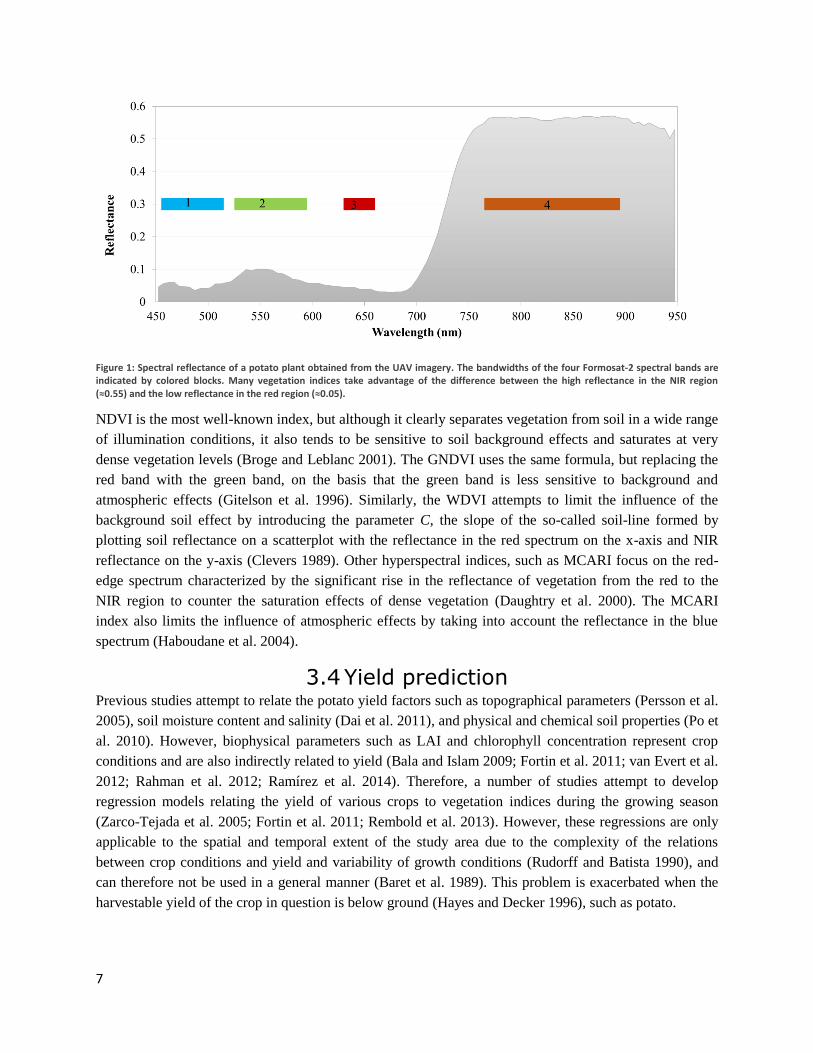
around 700 nm is characteristic of live green vegetation, and is known as the red-edge (Figure 1).
Vegetation indices take advantage of such characteristics, calculating ratios between spectral bands in
different regions to obtain an index which can be related to certain biophysical properties (Gilabert et al.
2010).
Vegetation indices are sensitive to variations in plant biophysical parameters while remaining robust to
external factors such as atmosphere, solar geometry, and soil background (Gilabert et al. 2010). However,
each vegetation index is a simplification of original surface reflectance, and therefore portray only a part
of the information contained within the original bands (Govaerts et al. 1999). Furthermore, many
vegetation indices relating red and NIR spectral bands display saturation at higher vegetation densities
(Myneni et al. 1995) and are dependent on canopy structure and land cover (Gilabert et al. 2010).
7
Figure 1: Spectral reflectance of a potato plant obtained from the UAV imagery. The bandwidths of the four Formosat-2 spectral bands are indicated by colored blocks. Many vegetation indices take advantage of the difference between the high reflectance in the NIR region (≈0.55) and the low reflectance in the red region (≈0.05).
NDVI is the most well-known index, but although it clearly separates vegetation from soil in a wide range
of illumination conditions, it also tends to be sensitive to soil background effects and saturates at very
dense vegetation levels (Broge and Leblanc 2001). The GNDVI uses the same formula, but replacing the
red band with the green band, on the basis that the green band is less sensitive to background and
atmospheric effects (Gitelson et al. 1996). Similarly, the WDVI attempts to limit the influence of the
background soil effect by introducing the parameter C, the slope of the so-called soil-line formed by
plotting soil reflectance on a scatterplot with the reflectance in the red spectrum on the x-axis and NIR
reflectance on the y-axis (Clevers 1989). Other hyperspectral indices, such as MCARI focus on the red-
edge spectrum characterized by the significant rise in the reflectance of vegetation from the red to the
NIR region to counter the saturation effects of dense vegetation (Daughtry et al. 2000). The MCARI
index also limits the influence of atmospheric effects by taking into account the reflectance in the blue
spectrum (Haboudane et al. 2004).
3.4 Yield prediction Previous studies attempt to relate the potato yield factors such as topographical parameters (Persson et al.
2005), soil moisture content and salinity (Dai et al. 2011), and physical and chemical soil properties (Po et
al. 2010). However, biophysical parameters such as LAI and chlorophyll concentration represent crop
conditions and are also indirectly related to yield (Bala and Islam 2009; Fortin et al. 2011; van Evert et al.
2012; Rahman et al. 2012; Ramírez et al. 2014). Therefore, a number of studies attempt to develop
regression models relating the yield of various crops to vegetation indices during the growing season
(Zarco-Tejada et al. 2005; Fortin et al. 2011; Rembold et al. 2013). However, these regressions are only
applicable to the spatial and temporal extent of the study area due to the complexity of the relations
between crop conditions and yield and variability of growth conditions (Rudorff and Batista 1990), and
can therefore not be used in a general manner (Baret et al. 1989). This problem is exacerbated when the
harvestable yield of the crop in question is below ground (Hayes and Decker 1996), such as potato.
8
Regression models developed for predicting agricultural yield often focus on using vegetation indices of
individual images, the maximum value during the growing season, cumulative values, or integrated values
(Rembold et al. 2013). For example, Bala and Islam (2009) related potato yield in India to NDVI, LAI
and the fraction of Photosynthetically Active Radiation (fPAR) data obtained from MODIS imagery.
They calculated the coefficient of determination (R2) between the three parameters for 19 MODIS images
to the yield, and developed a regression model in which the potato yield was based on the mean NDVI
during the growing season. Rahman et al. (2012) compared inter-annual potato yield variation to weekly
Vegetation Condition Indices (VCI) obtained from AVHRR imagery. Neale and Sivarajan (2011)
compared potato yield to the SAVI at three stages in the growing season, and the integrated SAVI during
the entire growing season. Each of these studies obtained linear regression models based on vegetation
indices which explained a large part of the yield variability.
9
Data and Methodology
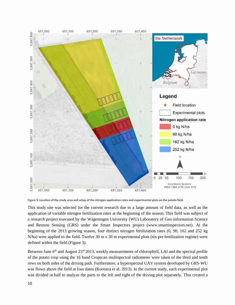
4.1 Study area A potato field along the border between the Netherlands and Belgium, near the Dutch village of Reusel
was selected for the current study (Figure 3). The field is located at 51°10’N, 5°19’W and has an area of
approximately 11 ha. The surrounding area is characterized by a temperate climate. The nearest
meteorological station is in Eindhoven, at a distance of 24 km from the potato field.
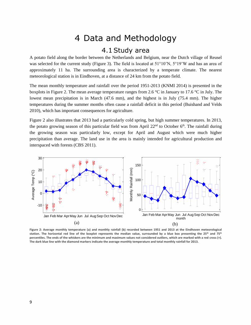
The mean monthly temperature and rainfall over the period 1951-2013 (KNMI 2014) is presented in the
boxplots in Figure 2. The mean average temperature ranges from 2.6 °C in January to 17.6 °C in July. The
lowest mean precipitation is in March (47.6 mm), and the highest is in July (75.4 mm). The higher
temperatures during the summer months often cause a rainfall deficit in this period (Buishand and Velds
2010), which has important consequences for agriculture.
Figure 2 also illustrates that 2013 had a particularly cold spring, but high summer temperatures. In 2013,
the potato growing season of this particular field was from April 22nd to October 6th. The rainfall during
the growing season was particularly low, except for April and August which were much higher
precipitation than average. The land use in the area is mainly intended for agricultural production and
interspaced with forests (CBS 2011).
(a)
(b)
Figure 2: Average monthly temperature (a) and monthly rainfall (b) recorded between 1951 and 2013 at the Eindhoven meteorological station. The horizontal red line of the boxplot represents the median value, surrounded by a blue box presenting the 25th and 75th percentiles. The ends of the whiskers are the minimum and maximum values not considered outliers, which are marked with a red cross (+). The dark blue line with the diamond markers indicate the average monthly temperature and total monthly rainfall for 2013.
-10
0
10
20
30
Jan Feb Mar AprMay Jun Jul AugSep Oct NovDec
Avera
ge T
em
p (
°C)
0
50
100
150
Jan Feb Mar AprMay Jun Jul AugSep Oct NovDecmonth
Month
ly R
ain
fall
(mm
)
10
Figure 3: Location of the study area and setup of the nitrogen application rates and experimental plots on the potato field.
This study site was selected for the current research due to a large amount of field data, as well as the
application of variable nitrogen fertilization rates at the beginning of the season. This field was subject of
a research project executed by the Wageningen University (WU) Laboratory of Geo-information Science
and Remote Sensing (GRS) under the Smart Inspectors project (www.smartinspectors.net). At the
beginning of the 2013 growing season, four distinct nitrogen fertilization rates (0, 90, 162 and 252 kg
N/ha) were applied to the field. Twelve 30 m x 30 m experimental plots (six per fertilization regime) were
defined within the field (Figure 3).
Between June 6th and August 23rd 2013, weekly measurements of chlorophyll, LAI and the spectral profile
of the potato crop using the 16 band Cropscan multispectral radiometer were taken of the third and tenth
rows on both sides of the driving path. Furthermore, a hyperspectral UAV system developed by GRS-WU
was flown above the field at four dates (Kooistra et al. 2013). In the current study, each experimental plot
was divided in half to analyze the parts to the left and right of the driving plot separately. This created a
11
larger number of plots with a smaller spatial scale to improve the statistical analysis between the satellite
imagery and field data. It also removed the tractor driving path from the experimental plots, as the lack of
vegetation on the driving path would affect the plot surface reflectance obtained from imagery. Therefore,
the current study makes use of 24 13 m x 30 m experimental plots.
4.2 Data
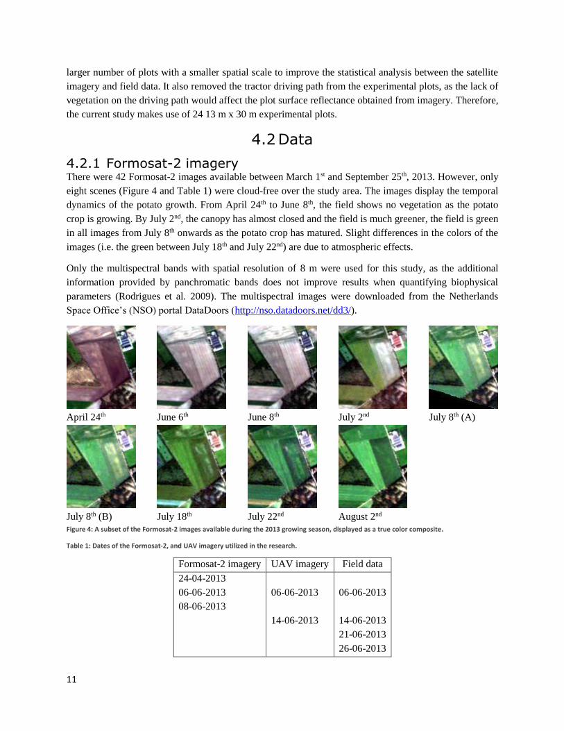
4.2.1 Formosat-2 imagery There were 42 Formosat-2 images available between March 1st and September 25th, 2013. However, only
eight scenes (Figure 4 and Table 1) were cloud-free over the study area. The images display the temporal
dynamics of the potato growth. From April 24th to June 8th, the field shows no vegetation as the potato
crop is growing. By July 2nd, the canopy has almost closed and the field is much greener, the field is green
in all images from July 8th onwards as the potato crop has matured. Slight differences in the colors of the
images (i.e. the green between July 18th and July 22nd) are due to atmospheric effects.
Only the multispectral bands with spatial resolution of 8 m were used for this study, as the additional
information provided by panchromatic bands does not improve results when quantifying biophysical
parameters (Rodrigues et al. 2009). The multispectral images were downloaded from the Netherlands
Space Office’s (NSO) portal DataDoors (http://nso.datadoors.net/dd3/).
April 24th
June 6th
June 8th
July 2nd
July 8th (A)
July 8th (B)
July 18th
July 22nd
August 2nd
Figure 4: A subset of the Formosat-2 images available during the 2013 growing season, displayed as a true color composite.
Table 1: Dates of the Formosat-2, and UAV imagery utilized in the research.
Formosat-2 imagery UAV imagery Field data
24-04-2013
06-06-2013
08-06-2013
06-06-2013
14-06-2013
06-06-2013
14-06-2013
21-06-2013
26-06-2013
12
Formosat-2 imagery UAV imagery Field data
02-07-2013
08-07-2013 (x2)
18-07-2013
22-07-2013
02-08-2013
05-07-2013
17-07-2013
05-07-2013
12-07-2013
17-07-2013
26-07-2013
31-07-2013
16-08-2013
23-08-2013
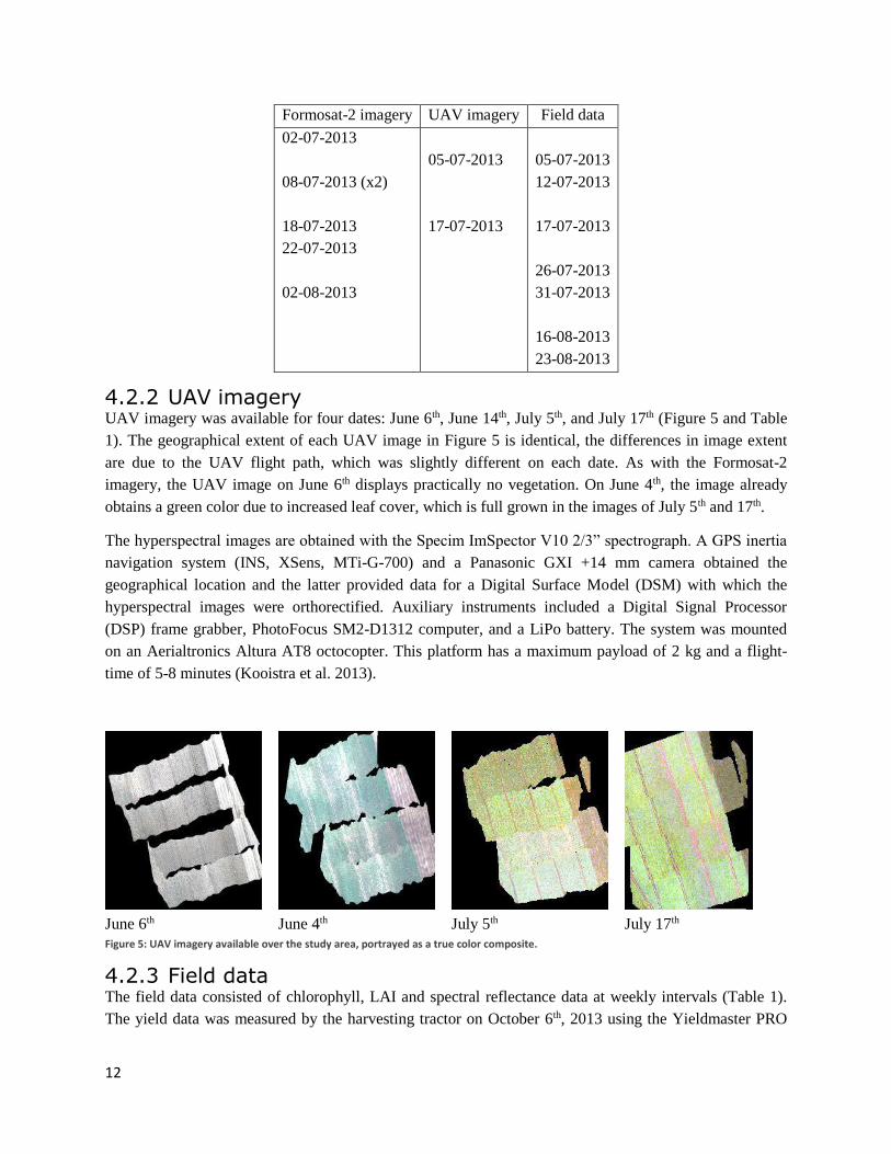
4.2.2 UAV imagery UAV imagery was available for four dates: June 6th, June 14th, July 5th, and July 17th (Figure 5 and Table
1). The geographical extent of each UAV image in Figure 5 is identical, the differences in image extent
are due to the UAV flight path, which was slightly different on each date. As with the Formosat-2
imagery, the UAV image on June 6th displays practically no vegetation. On June 4th, the image already
obtains a green color due to increased leaf cover, which is full grown in the images of July 5th and 17th.
The hyperspectral images are obtained with the Specim ImSpector V10 2/3” spectrograph. A GPS inertia
navigation system (INS, XSens, MTi-G-700) and a Panasonic GXI +14 mm camera obtained the
geographical location and the latter provided data for a Digital Surface Model (DSM) with which the
hyperspectral images were orthorectified. Auxiliary instruments included a Digital Signal Processor
(DSP) frame grabber, PhotoFocus SM2-D1312 computer, and a LiPo battery. The system was mounted
on an Aerialtronics Altura AT8 octocopter. This platform has a maximum payload of 2 kg and a flight-
time of 5-8 minutes (Kooistra et al. 2013).
June 6th
June 4th
July 5th
July 17th
Figure 5: UAV imagery available over the study area, portrayed as a true color composite.
4.2.3 Field data The field data consisted of chlorophyll, LAI and spectral reflectance data at weekly intervals (Table 1).
The yield data was measured by the harvesting tractor on October 6th, 2013 using the Yieldmaster PRO
13
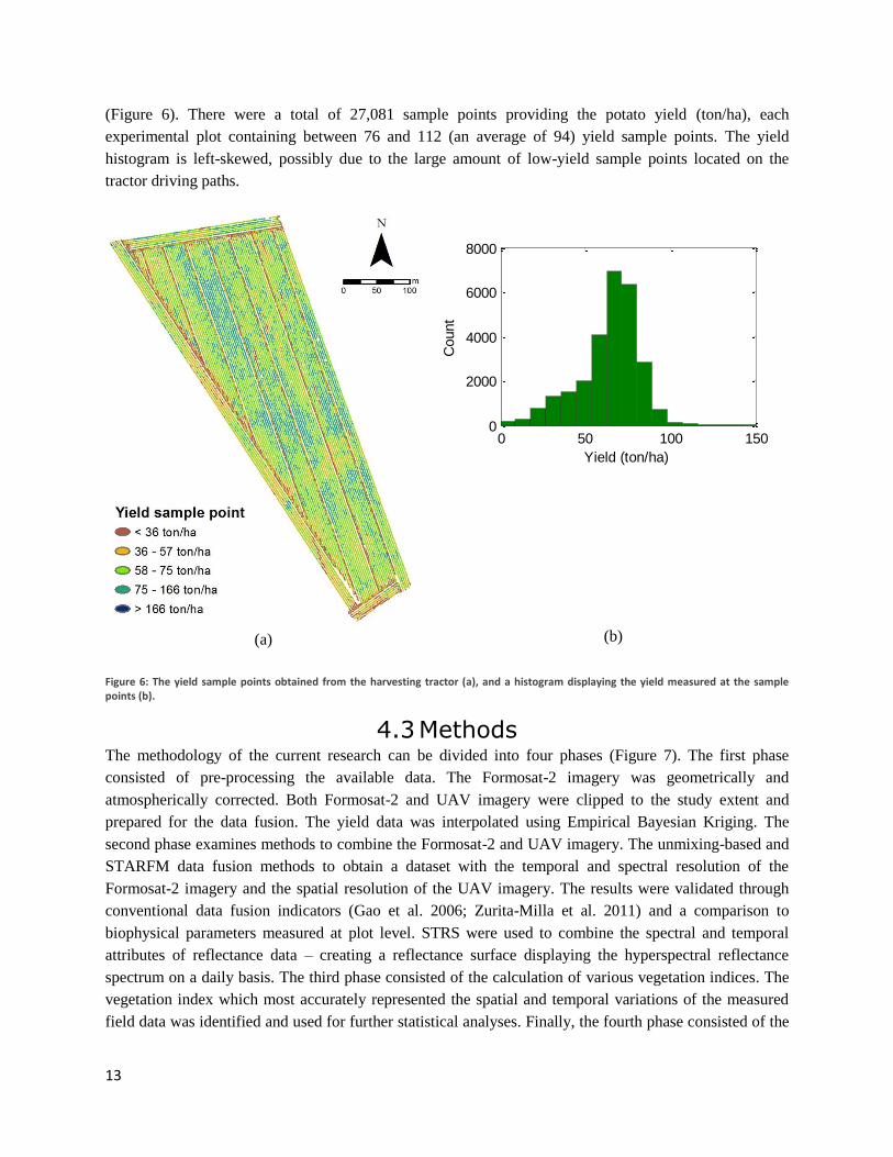
(Figure 6). There were a total of 27,081 sample points providing the potato yield (ton/ha), each
experimental plot containing between 76 and 112 (an average of 94) yield sample points. The yield
histogram is left-skewed, possibly due to the large amount of low-yield sample points located on the
tractor driving paths.
(a)
(b)
Figure 6: The yield sample points obtained from the harvesting tractor (a), and a histogram displaying the yield measured at the sample points (b).
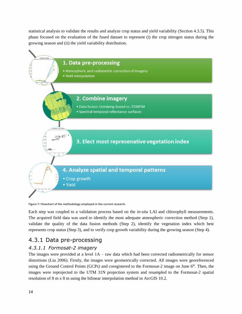
4.3 Methods The methodology of the current research can be divided into four phases (Figure 7). The first phase
consisted of pre-processing the available data. The Formosat-2 imagery was geometrically and
atmospherically corrected. Both Formosat-2 and UAV imagery were clipped to the study extent and
prepared for the data fusion. The yield data was interpolated using Empirical Bayesian Kriging. The
second phase examines methods to combine the Formosat-2 and UAV imagery. The unmixing-based and
STARFM data fusion methods to obtain a dataset with the temporal and spectral resolution of the
Formosat-2 imagery and the spatial resolution of the UAV imagery. The results were validated through
conventional data fusion indicators (Gao et al. 2006; Zurita-Milla et al. 2011) and a comparison to
biophysical parameters measured at plot level. STRS were used to combine the spectral and temporal
attributes of reflectance data – creating a reflectance surface displaying the hyperspectral reflectance
spectrum on a daily basis. The third phase consisted of the calculation of various vegetation indices. The
vegetation index which most accurately represented the spatial and temporal variations of the measured
field data was identified and used for further statistical analyses. Finally, the fourth phase consisted of the
0 50 100 1500
2000
4000
6000
8000
Yield (ton/ha)C
ount
14
statistical analysis to validate the results and analyze crop status and yield variability (Section 4.3.5). This
phase focused on the evaluation of the fused dataset to represent (i) the crop nitrogen status during the
growing season and (ii) the yield variability distribution.
Figure 7: Flowchart of the methodology employed in the current research.
Each step was coupled to a validation process based on the in-situ LAI and chlorophyll measurements.
The acquired field data was used to identify the most adequate atmospheric correction method (Step 1),
validate the quality of the data fusion methods (Step 2), identify the vegetation index which best
represents crop status (Step 3), and to verify crop growth variability during the growing season (Step 4).
4.3.1 Data pre-processing
4.3.1.1 Formosat-2 imagery
The images were provided at a level 1A – raw data which had been corrected radiometrically for sensor
distortions (Liu 2006). Firstly, the images were geometrically corrected. All images were georeferenced
using the Ground Control Points (GCPs) and coregistered to the Formosat-2 image on June 6th. Then, the
images were reprojected to the UTM 31N projection system and resampled to the Formosat-2 spatial
resolution of 8 m x 8 m using the bilinear interpolation method in ArcGIS 10.2.
15
The images were then converted from satellite Digital Number (DN) values to Top of Atmosphere (TOA)
radiances by using the physical gain parameters obtained from the metadata (Liu 2006). The images were
atmospherically corrected using DOS, ATCOR, QUAC, FLAASH, empirical line calibration and
radiometric normalization (see Appendix 1). The resulting surface reflectance were compared to the UAV
data, of which the QUAC method followed by an empirical line calibration and radiometrically
normalized to UAV data obtained the highest correlation and lowest root mean square error (RMSE).
Further information regarding this process can be found in Appendix 1.
A unique situation was presented as the study area was located in the overlap between two Formosat-2
scenes on July 8th. Thus, we have access to two distinct Formosat-2 images separated by four seconds. By
comparing the processed images of the study area, we can gain insight to the errors induced by the
Formosat-2 image processing chain. To this end, the RMSE and correlation between both images was
calculated. We hypothesize that these RMSE and correlations obtained in between the two Formosat-2
images on July 8th can be generalized to represent the errors of the other Formosat-2 images in the time
series.
4.3.1.2 UAV imagery
The radiometrically, atmospherically and geometrically corrected UAV imagery was provided by WU-
GRS. Pre-processing steps had included the conversion of raw data to reflectance, an empirical line
correction, and orthorectification using a DSM obtained from the camera onboard the octocopter. Further
details regarding the processing of UAV imagery can be found in Kooistra et al. (2013).
For each date, two UAV flights were made, each of which covered half the experimental plots. In the
current study, both images were mosaicked using ENVI 5.0 for each date. Invalid data at the edges of the
UAV imagery were masked, and the images from various dates were subsetted to the same extent.
4.3.1.3 Yield data
Statistical interpolation models such as kriging derive the spatial influence of proximal samples from the
characteristics of the dataset (Krivoruchko 2011). Unfortunately, kriging requires the interpolated data to
have a normal distribution, which the yield sample points are not as the histogram is bounded to positive
values and is left-skewed (Figure 6b). Therefore, the Empirical Bayesian Kriging (EBK) was used to
interpolate the yield data.
The EBK method provides accurate interpolations even when using non-stationary and non-Gaussian data
(Pilz and Spöck 2008; Krivoruchko and Gribov 2014). Firstly, outliers were identified in the histogram
and removed from the dataset. The EBK method was then applied using the Geostatistical Wizard
function of ArcGIS 10.2. The prediction quality was analyzed using the mean prediction error, the RMSE,
and the root-mean-square standardized error (RMSSE). The RMSSE divides the prediction error by the
standard deviation and normalizes it (Eq. 1.). Therefore, an RMSSE value greater than one indicates an
underestimation of data variability, and an RMSSE less than one indicates an overestimation of data
variability. The yield prediction and model prediction errors were exported to raster format with the same
spatial resolution and extent as the UAV imagery.
16
𝑅𝑀𝑆𝑆𝐸 = √∑ [(𝑦�̂� − 𝑦𝑖)/𝜎]2𝑛
𝑖=1
𝑛
Eq. 1.
Where 𝑦𝑖 is the yield measured at a sample point, 𝑦�̂� is the predicted yield at that point, 𝜎 is the standard
deviation of the measured yield, and 𝑛 is the number of points.
4.3.2 Data Fusion Optimal input parameters were determined for both fusion algorithms (Appendix 2) and utilized to apply
data fusion to each Formosat-2 image. Each time, the Formosat-2 image was utilized as the input
medium-resolution image for data fusion. The input high-resolution was always the most recent preceding
UAV image. By using only preceding UAV imagery we simulate a practical application in which data
fusion is applied during the growing season to monitor crop growth.
As mentioned before, the STARFM method requires a base medium- and high-resolution image pair on
the same date. In the current study, coincident Formosat-2 imagery was only available for two dates (June
6th and July 18th). Therefore, only the June 6th and July 17th UAV images can be included in the time
series through STARFM fusion. However, the unmixing method only requires an input UAV image, no
corresponding Formosat-2 image is needed. Therefore, all four UAV images were used as input for the
unmixing-based method.
4.3.3 STRS
4.3.3.1 Theoretical basis
4.3.3.1.1 Spectral interpolation: Bayesian imputation Proximal hyperspectral bands often display a high covariance (Mewes et al. 2009). Therefore, given the a
priori covariance of hyperspectral UAV spectral bands, the mean reflectance and distribution at the
known Formosat-2 wavelengths, a 101-band reflectance spectrum can be inferred using Bayesian
imputation. Thus, rather than fitting the four Formosat-2 spectral bands with a smooth spline
interpolation, for example, the physical reflectance characteristics of vegetation are mimicked to create a
realistic reflectance spectrum.
Suppose 𝒙𝒗𝒊 represents the surface reflectance at the Formosat-2 wavelengths and 𝒙𝒉𝒊
represents the
unknown surface reflectance at the 5 nm intervals between 450 and 950 nm (corresponding to the UAV
imagery) at date i. The distributions are jointly Gaussian, defined as follows:
𝑝(𝑥ℎ) = 𝒩(𝑥ℎ|𝝁𝒉, 𝚺𝒉𝒉) Eq. 2.
𝑝(𝑥𝑣) = 𝒩(𝑥𝑣|𝝁𝒗, 𝚺𝒗𝒗) Eq. 3.
Given the a priori mean and distribution of the Formosat-2 spectral reflectance (𝝁𝒗, 𝚺𝒗𝒗 ), and the
covariance matrix 𝚺 of the UAV spectra, the posterior conditional distribution can be obtained:
𝑝(𝑥ℎ𝑖|𝑥𝑣𝑖
) = 𝒩(𝑥𝑖|𝜇(ℎ|𝑣), Σℎ|𝑣)
Eq. 4.
𝝁(𝑥ℎ𝑖
|𝑥𝑣𝑖)
= 𝝁𝒉 + 𝚺𝒉𝒗𝚺𝒗𝒗−𝟏(𝑥𝑣 − 𝝁𝒗) Eq. 5.
17
𝚺(𝑥ℎ𝑖
|𝑥𝑣𝑖)
= 𝚺𝒉𝒉 − 𝚺𝒉𝒗𝚺𝒗𝒗−𝟏𝚺𝒗𝒉 Eq. 6.
From the posterior mean and distribution (𝝁(𝑥ℎ𝑖
|𝑥𝑣𝑖), 𝚺
(𝑥ℎ𝑖|𝑥𝑣𝑖
)), the missing spectral value is inferred.
𝑥𝑖𝑗 = 𝔼[𝑥𝑗|𝒙𝒗𝒊, 𝜽] Eq. 7.
Although hyperspectral bands display a high covariance between wavelengths, the nature of this
covariance will vary depending on the surface properties, i.e. soil vs. vegetation. Therefore, it is important
to select adequate a priori 𝝁𝒗 and 𝚺𝒗𝒗. The study area of the current application consists of a potato field,
so the endmembers within the image range from soil to green vegetation in various stages of growth. It is
assumed that the surface spectra within the boundaries of the STRS are represented within the available
UAV imagery.
4.3.3.1.2 Temporal Interpolation: Bayesian inference Previous studies regarding STRS apply standard 2D interpolation techniques to combine the spectral
information of various sensors (Mello et al. 2013; Villa et al. 2013). However, in practice imagery
obtained from differing sensors often present slightly different spectral reflectance values due to differing
wavelengths, bandwidths, radiometric precision, solar geometry and processing chains (Song and
Woodcock 2003), etc. Such inconsistencies may degrade the quality of the interpolated surface. An
alternative methodology is presented here, which interpolates the temporal dynamics of surface
reflectance through a Bayesian inference method.
This method infers a vector of true spectral reflectance x from a number of noisy observations y. The
mathematical formulation is set up as a linear Gaussian system, defining the error as having a normal
distribution:
𝑦 = 𝑨𝑥 + 𝜖 Eq. 8.
𝜖~ 𝒩(0, Σ𝑦), Σy = 𝜎2𝐼 Eq. 9.
In these equations, x represents the vector of true reflectance values, y is the vector of UAV and
Formosat-2 observations of this vector. 𝑨 is a logical NxD matrix of the N number of observations, or
available images, and D is the length of the date vector which will be interpolated. This matrix A is used
to select the dates for which images are available. The noise is assumed to have normal Gaussian
distribution (Eq. 9.) with a mean 0 and distribution equal to the observation noise 𝜎2 multiplied by an
identity matrix 𝐼.
The prior, x, is also defined as a Gaussian distribution (Eq. 10). The temporal profile is assumed to be
smooth, meaning that the value of x at date j is the average of its neighbors (Eq. 11) altered by Gaussian
noise (Eq. 12).
𝑝(𝑦|𝑥) = 𝒩(𝜇𝑦|𝑥 , Σ𝑥) Eq. 10.
𝜇𝑦|𝑥 = −𝑳1𝑇𝑳2𝒙 Eq. 11.
18
Σx = (𝜆2𝑳𝑇𝑳)−1 Eq. 12.
𝑳 =
1
2(
−1 2 −1…
−1 2 −1
) Eq. 13.
Where 𝑳 is a tri-diagonal matrix (Eq. 13) which selects the central observation as well as the previous and
following observations. By multiplying this matrix by the prior precision 𝜆 , the user can define the
strength of the prior distribution. If the user defines a prior precision 𝜆 relatively high compared to the
uncertainty of the surface reflectance data (𝜆 ≥ 𝜎2), the resulting temporal profile will be relatively
smooth. However, if the user defines a prior precision which is lower (𝜆 < 𝜎2 ), the weight of the
observations will be relatively higher and the temporal profile will adjust more to the imagery reflectance.
More information regarding the formulations of Bayesian imputation and inference can be found in
Murphy (2012).
In the current application, the uncertainty 𝜎2 was obtained from the standard deviation of spectral
measurements on the experimental plot. The uncertainty of the Formosat-2 spectra contained an
additional error: the variance of the posterior distribution in the imputation step (Eq. 14).
𝜎𝐹2𝑡𝑜𝑡 = √𝜎𝐹2 + 𝚺(𝑥ℎ𝑖
|𝑥𝑣𝑖) Eq. 14.
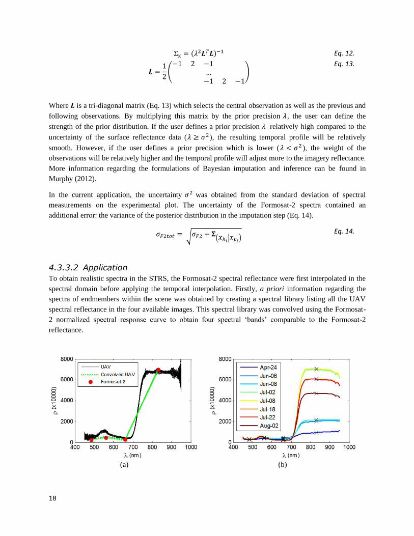
4.3.3.2 Application
To obtain realistic spectra in the STRS, the Formosat-2 spectral reflectance were first interpolated in the
spectral domain before applying the temporal interpolation. Firstly, a priori information regarding the
spectra of endmembers within the scene was obtained by creating a spectral library listing all the UAV
spectral reflectance in the four available images. This spectral library was convolved using the Formosat-
2 normalized spectral response curve to obtain four spectral ‘bands’ comparable to the Formosat-2
reflectance.
(a)
(b)
19
Figure 8: Illustrative figures indicating the spectral imputation method. (a) The Formosat-2 reflectance (red dot), closest samples from the UAV spectral library (black), and UAV reflectance convolved using the Formosat-2 spectral response function (green). (b) The Formosat-2 spectra imputed to 101 bands on various dates. Note how the characteristic vegetation spectrum is preserved.
For each experimental plot for each Formosat-2 image, 100 similar UAV spectra were selected from the
convolved spectral library Figure 8. The average, standard deviation and covariance was calculated for
each of the hyperspectral UAV bands of these 100 samples, and used as the a priori input for Bayesian
imputation. Selecting the a priori information separately for each experimental plot allows the imputed
spectra to represent spatial and temporal variation – i.e. it differentiates between plots with low vegetation
growth and a close canopy, allowing for a more accurate interpolation. It is important to note that this
methodology assumes that the spectral signatures within the spectral library are representative all the
spectra in the STRS. In the current situation, there is a large number of sample spectra (n=73,132), and
the library adequately represents the variation in crop growth which is expected to be present within the
experimental plot STRS.
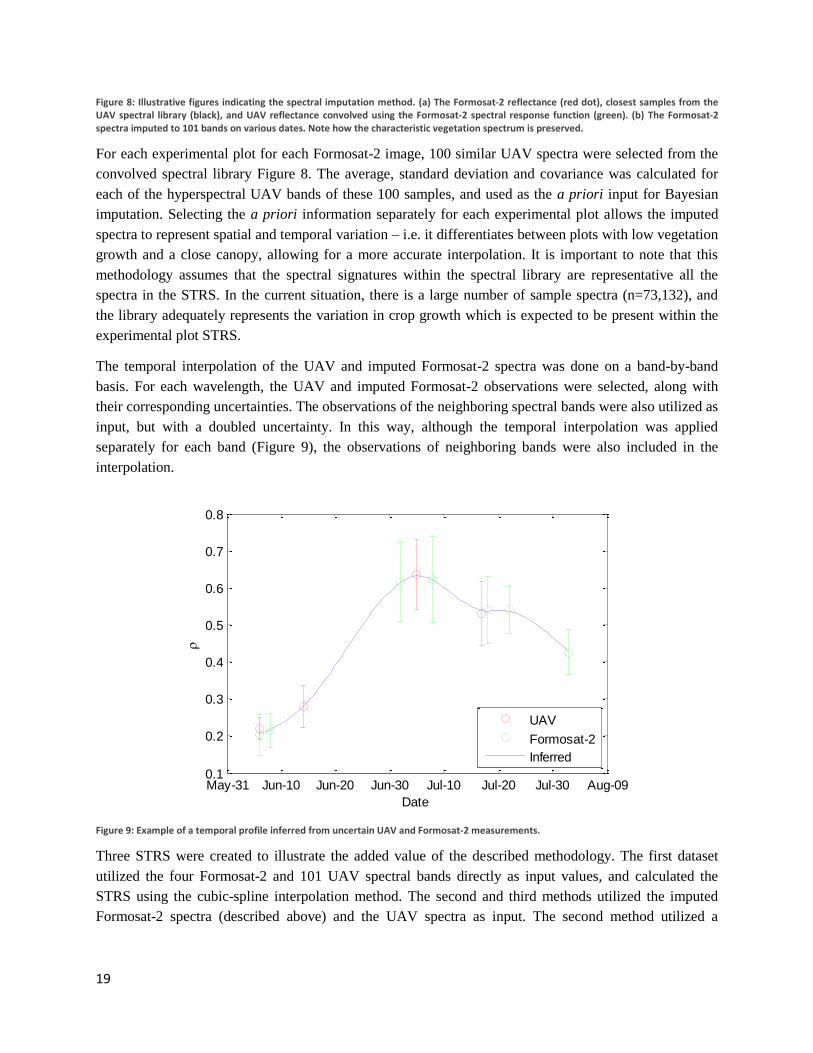
The temporal interpolation of the UAV and imputed Formosat-2 spectra was done on a band-by-band
basis. For each wavelength, the UAV and imputed Formosat-2 observations were selected, along with
their corresponding uncertainties. The observations of the neighboring spectral bands were also utilized as
input, but with a doubled uncertainty. In this way, although the temporal interpolation was applied
separately for each band (Figure 9), the observations of neighboring bands were also included in the
interpolation.
Figure 9: Example of a temporal profile inferred from uncertain UAV and Formosat-2 measurements.
Three STRS were created to illustrate the added value of the described methodology. The first dataset
utilized the four Formosat-2 and 101 UAV spectral bands directly as input values, and calculated the
STRS using the cubic-spline interpolation method. The second and third methods utilized the imputed
Formosat-2 spectra (described above) and the UAV spectra as input. The second method utilized a
May-31 Jun-10 Jun-20 Jun-30 Jul-10 Jul-20 Jul-30 Aug-090.1
0.2
0.3
0.4
0.5
0.6
0.7
0.8
Date
UAV
Formosat-2
Inferred
20
standard cubic spline interpolation method, whereas the third utilized the Bayesian approach method
consisting of spectral imputation followed by temporal inference as described previously.
4.3.4 Vegetation indices The third phase consisted of the calculation of various vegetation indices to prepare for the statistical
comparison of the images to the field and yield data. The current study applies a number of multispectral
and hyperspectral vegetation indices (Appendix 3). The vegetation index with the highest correlation to
LAI and chlorophyll data measured at the field level was selected for the subsequent analysis steps. A
number of multi- and hyperspectral vegetation indices were also calculated from the Bayesian-theory
based STRS.
To compare the fused and STRS datasets to the reference field data, the WDVI was also calculated from
the Cropscan multispectral radiometer field measurements, henceforth known as field WDVI. It should
also be noted that the correlations were calculated on four dates for the fused imagery dataset, and nine
dates for the STRS – due to the availability of coinciding field data.
4.3.5 Statistical analyses The statistical analysis of the current study addresses the following four questions: (1) Can the results of
data fusion and STRS be validated by field data? (2) Can vegetation indices be used to identify effects of
different nitrogen fertilization rates on crop growth during the growing season? And (3) can yield
variability be explained by crop growth parameters obtained from the image sets?
The first question requires validating the results of data fusion and STRS using the field data. The WDVI
(Appendix 3) was selected because previous studies with this UAV imagery indicated a good correlation
to the field LAI data (Kooistra et al. 2013). The WDVI was calculated for the fused datasets on the
reference dates: June 6th, July 5th, July 18th, and August 2nd. It was assumed that biophysical parameters
did not change significantly within a three day interval (e.g. between the Formosat-2 imagery of July 5th
and the field data of July 2nd and August 2nd vs. July 31st). These values were then compared to the
corresponding vegetation indices, chlorophyll, and LAI measured at the field level using the RMSE and
Spearman’s correlation coefficient. Similarly, the validation of the STRS calculated Spearman’s
correlation coefficient between the WDVI and MCARI (Appendix 3) vegetation indices obtained from
the STRS on all nine dates for which field data was available.
Regarding the second question, the vegetation index displaying the highest correlation to the biophysical
parameters measured at field level were used to create a temporal profile for each experimental plot. The
ability of the fused images to identify crop status variability due to differing initial nitrogen fertilization
rates was analyzed using a statistical variance test. A Kruskal-Wallis statistical test (Sheskin 2003) was
applied in Matlab R2012b to determine whether the vegetation index variance is significantly different
between the nitrogen application rate regimes. This provides insight to whether the nitrogen application
rates cause significant differences in crop growth, and at which dates such differences were visible.
The third question attempted to relate the yield variability to biophysical parameters during the growing
season. Again, a grouped Kruskal-Wallis test was applied to determine if the four different fertilization
regimes caused differences in yield, and which regime obtained the highest mean yield. Then, a stepwise
multivariate regression analysis (Fidell and Tabachnik 2012) was applied in IBM SPSS Statistics 22 to
21
determine the relation between the yield and a number of independent parameters at experimental plot
level. The entry threshold for a variable was p=0.05, and the exit threshold of the stepwise regression was
p=0.10.
Ten regression models were developed, based on differing input parameters. The first two models were
based on the measured field data. It was hypothesized that the first model, based on the LAI and
chlorophyll measurements, would explain the largest amount of yield variability, as these parameters are
direct indicators of crop status. The second model used parameters based on the GNDVI measured at field
level. It was hypothesized that this gives an indication of the largest amount of yield variability which can
be explained based on vegetation indices rather than biophysical parameters. The other eight models were
based on the following parameters obtained from either the unmixing-based, Formosat-2, or UAV images
or the STRS:
1. The GNDVI of each available image,
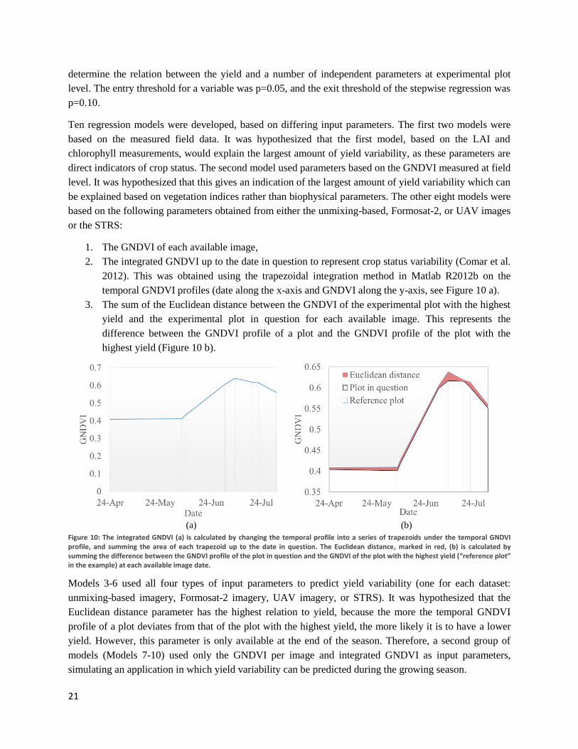
2. The integrated GNDVI up to the date in question to represent crop status variability (Comar et al.
2012). This was obtained using the trapezoidal integration method in Matlab R2012b on the
temporal GNDVI profiles (date along the x-axis and GNDVI along the y-axis, see Figure 10 a).
3. The sum of the Euclidean distance between the GNDVI of the experimental plot with the highest
yield and the experimental plot in question for each available image. This represents the
difference between the GNDVI profile of a plot and the GNDVI profile of the plot with the
highest yield (Figure 10 b).
(a) (b)
Figure 10: The integrated GNDVI (a) is calculated by changing the temporal profile into a series of trapezoids under the temporal GNDVI profile, and summing the area of each trapezoid up to the date in question. The Euclidean distance, marked in red, (b) is calculated by summing the difference between the GNDVI profile of the plot in question and the GNDVI of the plot with the highest yield (“reference plot” in the example) at each available image date.
Models 3-6 used all four types of input parameters to predict yield variability (one for each dataset:
unmixing-based imagery, Formosat-2 imagery, UAV imagery, or STRS). It was hypothesized that the
Euclidean distance parameter has the highest relation to yield, because the more the temporal GNDVI
profile of a plot deviates from that of the plot with the highest yield, the more likely it is to have a lower
yield. However, this parameter is only available at the end of the season. Therefore, a second group of
models (Models 7-10) used only the GNDVI per image and integrated GNDVI as input parameters,
simulating an application in which yield variability can be predicted during the growing season.
22
Results
5.1 Data pre-processing
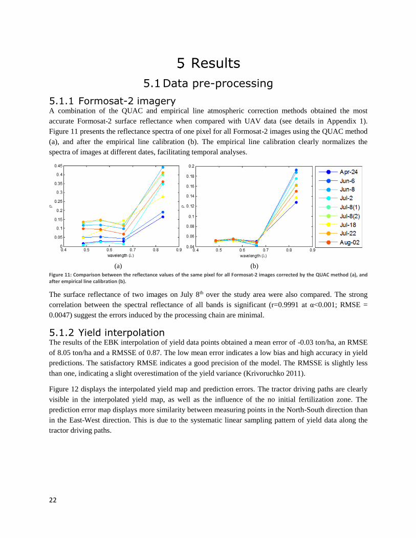
5.1.1 Formosat-2 imagery A combination of the QUAC and empirical line atmospheric correction methods obtained the most
accurate Formosat-2 surface reflectance when compared with UAV data (see details in Appendix 1).
Figure 11 presents the reflectance spectra of one pixel for all Formosat-2 images using the QUAC method
(a), and after the empirical line calibration (b). The empirical line calibration clearly normalizes the
spectra of images at different dates, facilitating temporal analyses.
(a) (b)
Figure 11: Comparison between the reflectance values of the same pixel for all Formosat-2 images corrected by the QUAC method (a), and after empirical line calibration (b).
The surface reflectance of two images on July 8th over the study area were also compared. The strong
correlation between the spectral reflectance of all bands is significant (r=0.9991 at α<0.001; RMSE =
0.0047) suggest the errors induced by the processing chain are minimal.
5.1.2 Yield interpolation The results of the EBK interpolation of yield data points obtained a mean error of -0.03 ton/ha, an RMSE
of 8.05 ton/ha and a RMSSE of 0.87. The low mean error indicates a low bias and high accuracy in yield
predictions. The satisfactory RMSE indicates a good precision of the model. The RMSSE is slightly less
than one, indicating a slight overestimation of the yield variance (Krivoruchko 2011).
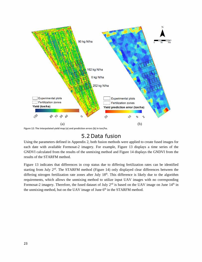
Figure 12 displays the interpolated yield map and prediction errors. The tractor driving paths are clearly
visible in the interpolated yield map, as well as the influence of the no initial fertilization zone. The
prediction error map displays more similarity between measuring points in the North-South direction than
in the East-West direction. This is due to the systematic linear sampling pattern of yield data along the
tractor driving paths.
23
(a) (b)
Figure 12: The interpolated yield map (a) and prediction errors (b) in ton/ha.
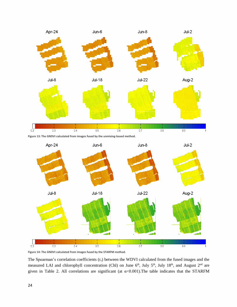
5.2 Data fusion Using the parameters defined in Appendix 2, both fusion methods were applied to create fused images for
each date with available Formosat-2 imagery. For example, Figure 13 displays a time series of the
GNDVI calculated from the results of the unmixing method and Figure 14 displays the GNDVI from the
results of the STARFM method.
Figure 13 indicates that differences in crop status due to differing fertilization rates can be identified
starting from July 2nd. The STARFM method (Figure 14) only displayed clear differences between the
differing nitrogen fertilization rate zones after July 18th. This difference is likely due to the algorithm
requirements, which allows the unmixing method to utilize input UAV images with no corresponding
Formosat-2 imagery. Therefore, the fused dataset of July 2nd is based on the UAV image on June 14th in
the unmixing-method, but on the UAV image of June 6th in the STARFM method.
24
Figure 13: The GNDVI calculated from images fused by the unmixing-based method.
Figure 14: The GNDVI calculated from images fused by the STARFM method.
The Spearman’s correlation coefficients (rs) between the WDVI calculated from the fused images and the
measured LAI and chlorophyll concentration (Chl) on June 6th, July 5th, July 18th, and August 2nd are
given in Table 2. All correlations are significant (at α<0.001).The table indicates that the STARFM
25
WDVI has the lowest correlation to all field data. The correlation coefficient of the unmixing-based
WDVI (rs=0.802) to the field data is comparable to the correlations obtained from the original UAV
(rs=0.847) and Formosat-2 (rs=0.808) data. The RMSE of the unmixing-based method is equal to that of
the Formosat-2 WDVI (0.310) whereas the STARFM method the same RMSE as UAV WDVI (0.214).
This is logical as the unmixing-based method obtains spectral reflectance from the Formosat-2 imagery,
whereas the STARFM method obtains spectral reflectance from the UAV imagery.
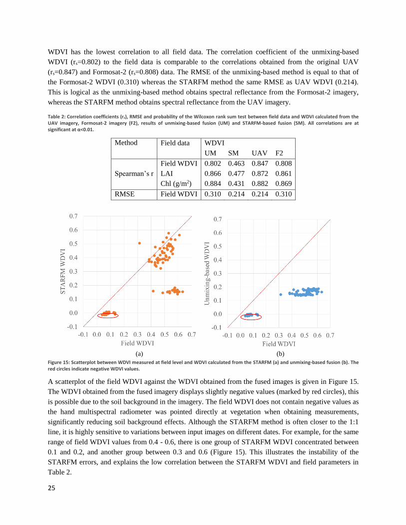
Table 2: Correlation coefficients (rs), RMSE and probability of the Wilcoxon rank sum test between field data and WDVI calculated from the UAV imagery, Formosat-2 imagery (F2), results of unmixing-based fusion (UM) and STARFM-based fusion (SM). All correlations are at significant at α<0.01.
Method Field data WDVI
UM SM UAV F2
Field WDVI 0.802 0.463 0.847 0.808
Spearman’s r LAI 0.866 0.477 0.872 0.861
Chl (g/m2) 0.884 0.431 0.882 0.869
RMSE Field WDVI 0.310 0.214 0.214 0.310
(a) (b)
Figure 15: Scatterplot between WDVI measured at field level and WDVI calculated from the STARFM (a) and unmixing-based fusion (b). The red circles indicate negative WDVI values.
A scatterplot of the field WDVI against the WDVI obtained from the fused images is given in Figure 15.
The WDVI obtained from the fused imagery displays slightly negative values (marked by red circles), this
is possible due to the soil background in the imagery. The field WDVI does not contain negative values as
the hand multispectral radiometer was pointed directly at vegetation when obtaining measurements,
significantly reducing soil background effects. Although the STARFM method is often closer to the 1:1
line, it is highly sensitive to variations between input images on different dates. For example, for the same
range of field WDVI values from 0.4 - 0.6, there is one group of STARFM WDVI concentrated between
0.1 and 0.2, and another group between 0.3 and 0.6 (Figure 15). This illustrates the instability of the
STARFM errors, and explains the low correlation between the STARFM WDVI and field parameters in
Table 2.
26
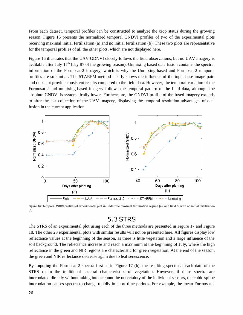
From each dataset, temporal profiles can be constructed to analyze the crop status during the growing
season. Figure 16 presents the normalized temporal GNDVI profiles of two of the experimental plots
receiving maximal initial fertilization (a) and no initial fertilization (b). These two plots are representative
for the temporal profiles of all the other plots, which are not displayed here.
Figure 16 illustrates that the UAV GDNVI closely follows the field observations, but no UAV imagery is
available after July 17th (day 87 of the growing season). Unmixing-based data fusion contains the spectral
information of the Formosat-2 imagery, which is why the Unmixing-based and Formosat-2 temporal
profiles are so similar. The STARFM method clearly shows the influence of the input base image pair,
and does not provide consistent results compared to the field data. However, the temporal variation of the
Formosat-2 and unmixing-based imagery follows the temporal pattern of the field data, although the
absolute GNDVI is systematically lower. Furthermore, the GNDVI profile of the fused imagery extends
to after the last collection of the UAV imagery, displaying the temporal resolution advantages of data
fusion in the current application.
(a) (b)
Figure 16: Temporal WDVI profiles of experimental plot AL under the maximal fertilization regime (a), and field BL with no initial fertilization (b).
5.3 STRS The STRS of an experimental plot using each of the three methods are presented in Figure 17 and Figure
18. The other 23 experimental plots with similar results will not be presented here. All figures display low
reflectance values at the beginning of the season, as there is little vegetation and a large influence of the
soil background. The reflectance increase and reach a maximum at the beginning of July, where the high
reflectance in the green and NIR regions are characteristic for green vegetation. At the end of the season,
the green and NIR reflectance decrease again due to leaf senescence.
By imputing the Formosat-2 spectra first as in Figure 17 (b), the resulting spectra at each date of the
STRS retain the traditional spectral characteristics of vegetation. However, if these spectra are
interpolated directly without taking into account the uncertainty of the individual sensors, the cubic spline
interpolation causes spectra to change rapidly in short time periods. For example, the mean Formosat-2
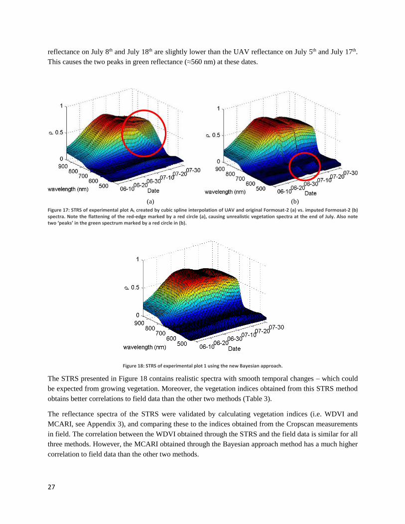
27
reflectance on July 8th and July 18th are slightly lower than the UAV reflectance on July 5th and July 17th.
This causes the two peaks in green reflectance (≈560 nm) at these dates.
(a) (b)
Figure 17: STRS of experimental plot AL created by cubic spline interpolation of UAV and original Formosat-2 (a) vs. imputed Formosat-2 (b) spectra. Note the flattening of the red-edge marked by a red circle (a), causing unrealistic vegetation spectra at the end of July. Also note two ‘peaks’ in the green spectrum marked by a red circle in (b).
Figure 18: STRS of experimental plot 1 using the new Bayesian approach.
The STRS presented in Figure 18 contains realistic spectra with smooth temporal changes – which could
be expected from growing vegetation. Moreover, the vegetation indices obtained from this STRS method
obtains better correlations to field data than the other two methods (Table 3).
The reflectance spectra of the STRS were validated by calculating vegetation indices (i.e. WDVI and
MCARI, see Appendix 3), and comparing these to the indices obtained from the Cropscan measurements
in field. The correlation between the WDVI obtained through the STRS and the field data is similar for all
three methods. However, the MCARI obtained through the Bayesian approach method has a much higher
correlation to field data than the other two methods.
28
Table 3: Correlation coefficient between vegetation indices obtained from STRS and the same vegetation index obtained in the field as well as the field LAI and canopy chlorophyll measurements.
WD
VI
Direct spline Impute + spline Bayesian approach
Field OSAVI 0.987 0.956 0.980
LAI 0.857 0.863 0.857
Canopy Chl 0.821 0.788 0.788
M
CA
RI
Direct spline Impute + spline Bayesian approach
Field MCARI 0.384 0.584 0.934
LAI 0.333 0.646 0.856
Canopy Chl 0.094 0.623 0.781
5.4 Vegetation indices The vegetation indices with the highest correlations to field LAI and canopy chlorophyll measurements
were selected for both the fused imagery and the STRS. Section 5.2 indicated that the unmixing-based
method provided fused images with more stable prediction errors, whereas the STARFM method had
highly variable prediction errors, as indicated in previous studies (Gevaert and García-Haro 2014).
Therefore, the unmixing-based method was used for further analyses regarding optimal vegetation
indices, temporal analysis and yield applications.
(a) (b)
Figure 19: The correlation of vegetation indices calculated from the unmixing-based imagery to the LAI (a) and canopy chlorophyll (b) measured at field level.
Figure 19 gives the correlation between various vegetation indices (calculated from the unmixing-based
images) and the LAI (Figure 19 a) and canopy chlorophyll (Figure 19 b) measured at field level for the
same four dates used above (see Section 5.2). The index of GNDVI displayed the highest correlation to
both LAI (rs=0.899) and canopy chlorophyll (rs=0.819). The other vegetation indices displayed
correlations above 0.859 to the LAI and above 0.726 to the canopy chlorophyll. It was concluded that the
GNDVI obtained from the unmixing-based imagery was most representative of the field data in the
current study, and was therefore used in the further analyses.
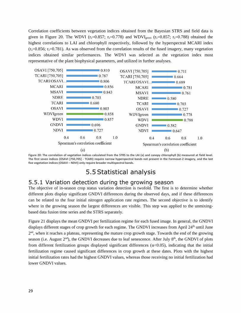
29
Correlation coefficients between vegetation indices obtained from the Bayesian STRS and field data is
given in Figure 20. The WDVI (rs=0.857; rs=0.778) and WDVIgreen (rs=0.857; rs=0.788) obtained the
highest correlations to LAI and chlorophyll respectively, followed by the hyperspectral MCARI index
(rs=0.856; rs=0.781). As was observed from the correlation results of the fused imagery, many vegetation
indices obtained similar performances. The WDVI was selected as the vegetation index most
representative of the plant biophysical parameters, and utilized in further analyses.
(a) (b)
Figure 20: The correlation of vegetation indices calculated from the STRS to the LAI (a) and canopy chlorophyll (b) measured at field level. The first seven indices (OSAVI [750,705] - TCARI) require narrow hyperspectral bands not present in the Formosat-2 imagery, and the last five vegetation indices (OSAVI – NDVI) only require broader multispectral bands.
5.5 Statistical analysis
5.5.1 Variation detection during the growing season The objective of in-season crop status variation detection is twofold. The first is to determine whether
different plots display significant GNDVI differences during the observed days, and if these differences
can be related to the four initial nitrogen application rate regimes. The second objective is to identify
where in the growing season the largest differences are visible. This step was applied to the unmixing-
based data fusion time series and the STRS separately.
Figure 21 displays the mean GNDVI per fertilization regime for each fused image. In general, the GNDVI
displays different stages of crop growth for each regime. The GNDVI increases from April 24th until June
2nd, when it reaches a plateau, representing the mature crop growth stage. Towards the end of the growing
season (i.e. August 2nd), the GNDVI decreases due to leaf senescence. After July 8th, the GNDVI of plots
from different fertilization groups displayed significant differences (α<0.05), indicating that the initial
fertilization regime caused significant differences in crop growth at these dates. Plots with the highest
initial fertilization rates had the highest GNDVI values, whereas those receiving no initial fertilization had
lower GNDVI values.
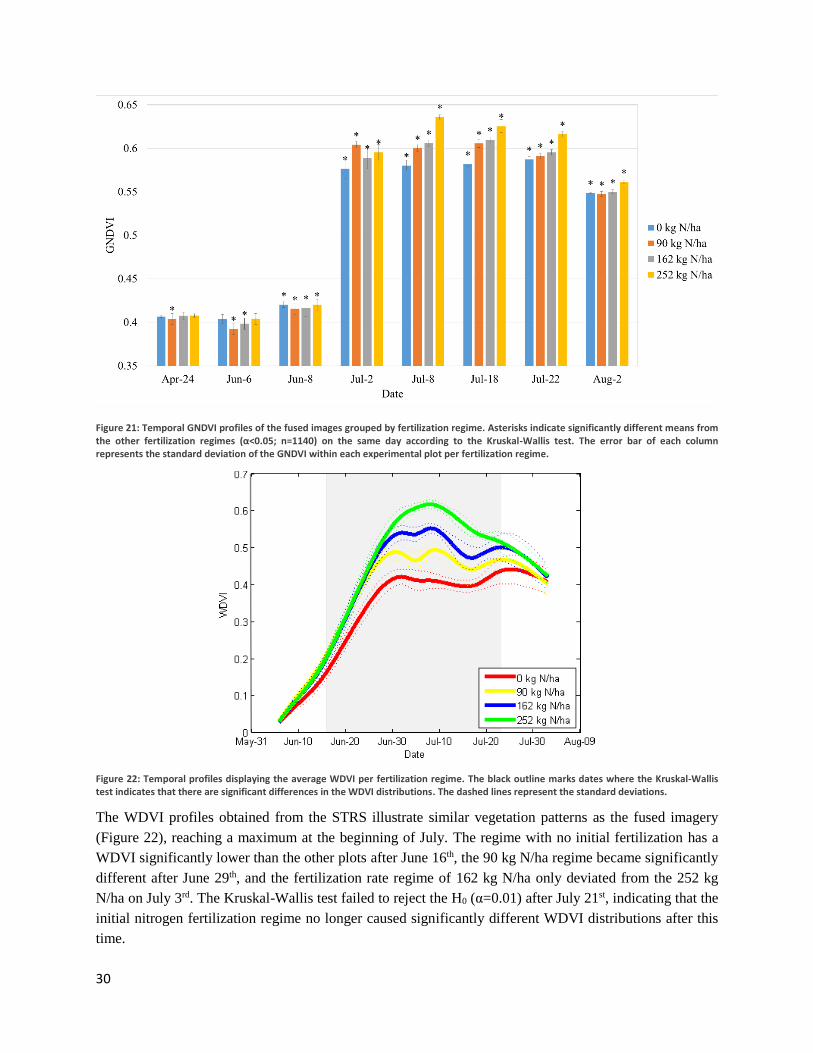
30
Figure 21: Temporal GNDVI profiles of the fused images grouped by fertilization regime. Asterisks indicate significantly different means from the other fertilization regimes (α<0.05; n=1140) on the same day according to the Kruskal-Wallis test. The error bar of each column represents the standard deviation of the GNDVI within each experimental plot per fertilization regime.
Figure 22: Temporal profiles displaying the average WDVI per fertilization regime. The black outline marks dates where the Kruskal-Wallis test indicates that there are significant differences in the WDVI distributions. The dashed lines represent the standard deviations.
The WDVI profiles obtained from the STRS illustrate similar vegetation patterns as the fused imagery
(Figure 22), reaching a maximum at the beginning of July. The regime with no initial fertilization has a
WDVI significantly lower than the other plots after June 16th, the 90 kg N/ha regime became significantly
different after June 29th, and the fertilization rate regime of 162 kg N/ha only deviated from the 252 kg
N/ha on July 3rd. The Kruskal-Wallis test failed to reject the H0 (α=0.01) after July 21st, indicating that the
initial nitrogen fertilization regime no longer caused significantly different WDVI distributions after this
time.
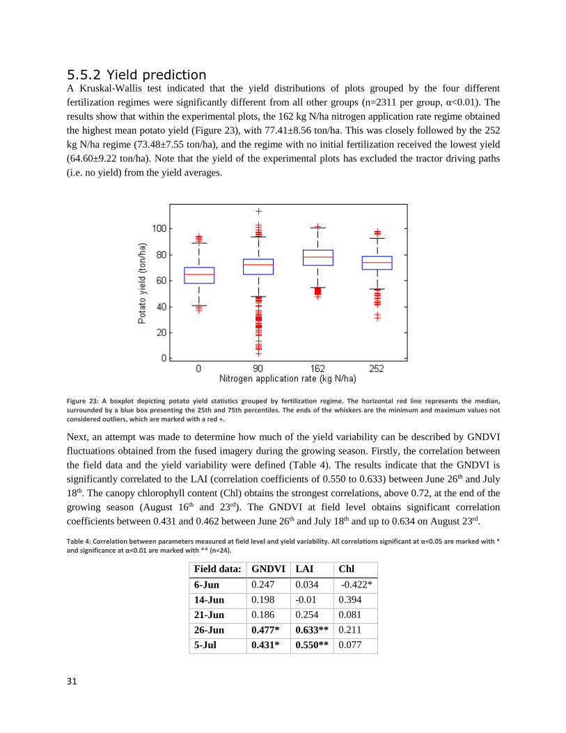
31
5.5.2 Yield prediction A Kruskal-Wallis test indicated that the yield distributions of plots grouped by the four different
fertilization regimes were significantly different from all other groups (n=2311 per group, α<0.01). The
results show that within the experimental plots, the 162 kg N/ha nitrogen application rate regime obtained
the highest mean potato yield (Figure 23), with 77.41±8.56 ton/ha. This was closely followed by the 252
kg N/ha regime (73.48±7.55 ton/ha), and the regime with no initial fertilization received the lowest yield
(64.60±9.22 ton/ha). Note that the yield of the experimental plots has excluded the tractor driving paths
(i.e. no yield) from the yield averages.
Figure 23: A boxplot depicting potato yield statistics grouped by fertilization regime. The horizontal red line represents the median, surrounded by a blue box presenting the 25th and 75th percentiles. The ends of the whiskers are the minimum and maximum values not considered outliers, which are marked with a red +.
Next, an attempt was made to determine how much of the yield variability can be described by GNDVI
fluctuations obtained from the fused imagery during the growing season. Firstly, the correlation between
the field data and the yield variability were defined (Table 4). The results indicate that the GNDVI is
significantly correlated to the LAI (correlation coefficients of 0.550 to 0.633) between June 26th and July
18th. The canopy chlorophyll content (Chl) obtains the strongest correlations, above 0.72, at the end of the
growing season (August 16th and 23rd). The GNDVI at field level obtains significant correlation
coefficients between 0.431 and 0.462 between June 26th and July 18th and up to 0.634 on August 23rd.
Table 4: Correlation between parameters measured at field level and yield variability. All correlations significant at α<0.05 are marked with * and significance at α<0.01 are marked with ** (n=24).
Field data: GNDVI LAI Chl
6-Jun 0.247 0.034 -0.422*
14-Jun 0.198 -0.01 0.394
21-Jun 0.186 0.254 0.081
26-Jun 0.477* 0.633** 0.211
5-Jul 0.431* 0.550** 0.077
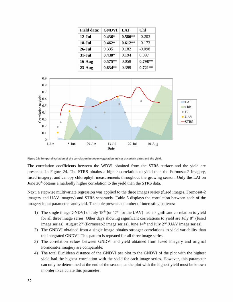
32
Field data: GNDVI LAI Chl
12-Jul 0.436* 0.580** -0.203
18-Jul 0.462* 0.612** -0.173
26-Jul 0.335 0.182 -0.098
31-Jul 0.430* 0.194 0.097
16-Aug 0.575** 0.058 0.798**
23-Aug 0.634** 0.399 0.721**
Figure 24: Temporal variation of the correlation between vegetation indices at certain dates and the yield.
The correlation coefficients between the WDVI obtained from the STRS surface and the yield are
presented in Figure 24. The STRS obtains a higher correlation to yield than the Formosat-2 imagery,
fused imagery, and canopy chlorophyll measurements throughout the growing season. Only the LAI on
June 26th obtains a markedly higher correlation to the yield than the STRS data.
Next, a stepwise multivariate regression was applied to the three images series (fused images, Formosat-2
imagery and UAV imagery) and STRS separately. Table 5 displays the correlation between each of the
imagery input parameters and yield. The table presents a number of interesting patterns:
1) The single image GNDVI of July 18th (or 17th for the UAV) had a significant correlation to yield
for all three image series. Other days showing significant correlations to yield are July 8th (fused
image series), August 2nd (Formosat-2 image series), June 14th and July 2nd (UAV image series).
2) The GNDVI obtained from a single image obtains stronger correlations to yield variability than
the integrated GNDVI. This pattern is repeated for all three image series.
3) The correlation values between GNDVI and yield obtained from fused imagery and original
Formosat-2 imagery are comparable.
4) The total Euclidean distance of the GNDVI per plot to the GNDVI of the plot with the highest
yield had the highest correlation with the yield for each image series. However, this parameter
can only be determined at the end of the season, as the plot with the highest yield must be known
in order to calculate this parameter.
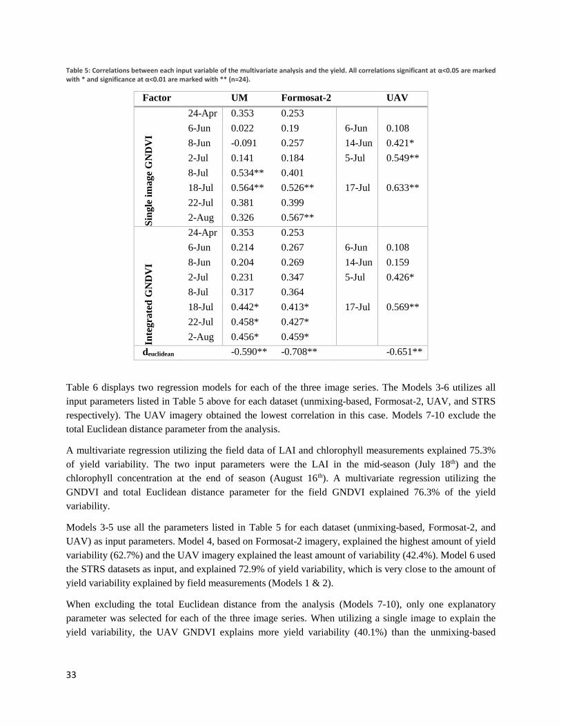
33
Table 5: Correlations between each input variable of the multivariate analysis and the yield. All correlations significant at α<0.05 are marked with * and significance at α<0.01 are marked with ** (n=24).
Factor UM Formosat-2 UAV
Sin
gle
im
ag
e G
ND
VI
24-Apr 0.353 0.253
6-Jun 0.022 0.19 6-Jun 0.108
8-Jun -0.091 0.257 14-Jun 0.421*
2-Jul 0.141 0.184 5-Jul 0.549**
8-Jul 0.534** 0.401
18-Jul 0.564** 0.526** 17-Jul 0.633**
22-Jul 0.381 0.399
2-Aug 0.326 0.567**
Inte
gra
ted
GN
DV
I
24-Apr 0.353 0.253
6-Jun 0.214 0.267 6-Jun 0.108
8-Jun 0.204 0.269 14-Jun 0.159
2-Jul 0.231 0.347 5-Jul 0.426*
8-Jul 0.317 0.364
18-Jul 0.442* 0.413* 17-Jul 0.569**
22-Jul 0.458* 0.427*
2-Aug 0.456* 0.459*
deuclidean -0.590** -0.708** -0.651**
Table 6 displays two regression models for each of the three image series. The Models 3-6 utilizes all
input parameters listed in Table 5 above for each dataset (unmixing-based, Formosat-2, UAV, and STRS
respectively). The UAV imagery obtained the lowest correlation in this case. Models 7-10 exclude the
total Euclidean distance parameter from the analysis.
A multivariate regression utilizing the field data of LAI and chlorophyll measurements explained 75.3%
of yield variability. The two input parameters were the LAI in the mid-season (July 18th) and the
chlorophyll concentration at the end of season (August 16th). A multivariate regression utilizing the
GNDVI and total Euclidean distance parameter for the field GNDVI explained 76.3% of the yield
variability.
Models 3-5 use all the parameters listed in Table 5 for each dataset (unmixing-based, Formosat-2, and
UAV) as input parameters. Model 4, based on Formosat-2 imagery, explained the highest amount of yield
variability (62.7%) and the UAV imagery explained the least amount of variability (42.4%). Model 6 used
the STRS datasets as input, and explained 72.9% of yield variability, which is very close to the amount of
yield variability explained by field measurements (Models 1 & 2).
When excluding the total Euclidean distance from the analysis (Models 7-10), only one explanatory
parameter was selected for each of the three image series. When utilizing a single image to explain the
yield variability, the UAV GNDVI explains more yield variability (40.1%) than the unmixing-based
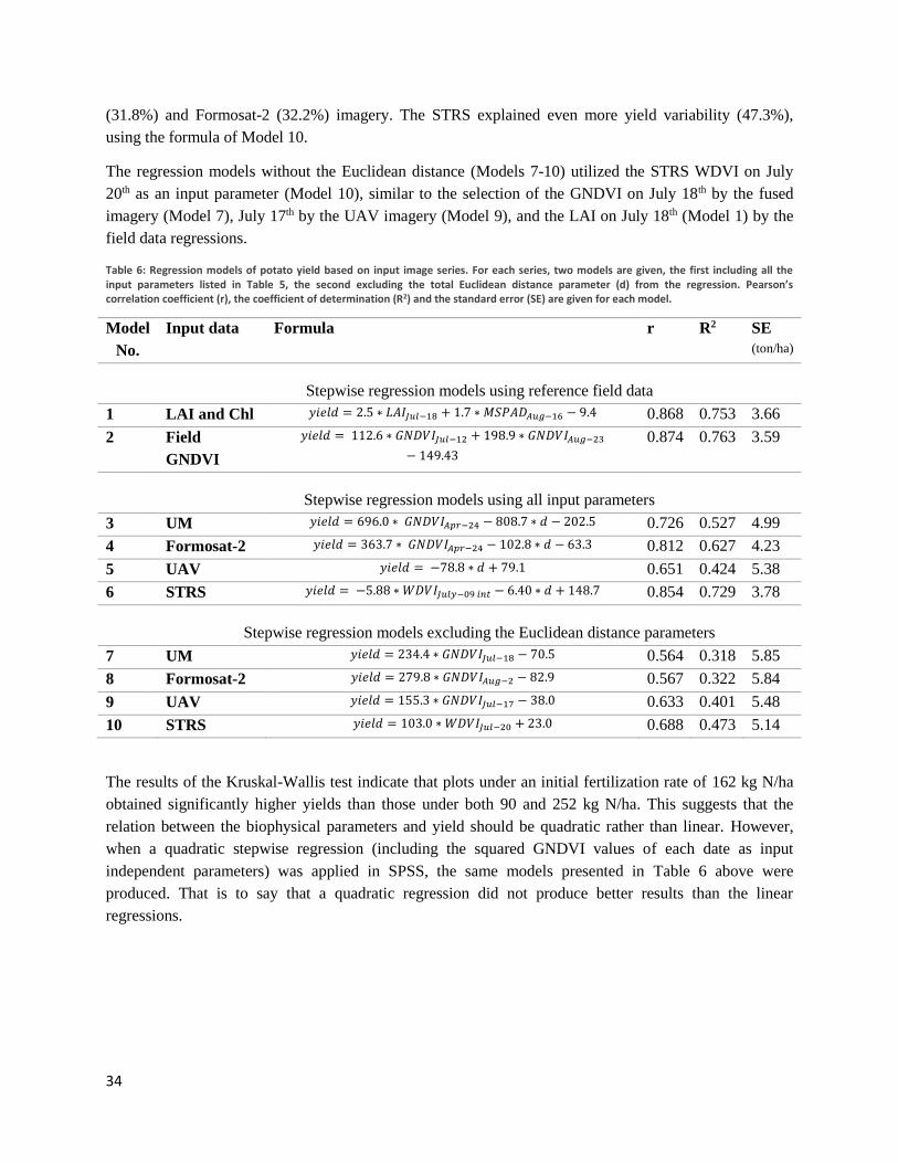
34
(31.8%) and Formosat-2 (32.2%) imagery. The STRS explained even more yield variability (47.3%),
using the formula of Model 10.
The regression models without the Euclidean distance (Models 7-10) utilized the STRS WDVI on July
20th as an input parameter (Model 10), similar to the selection of the GNDVI on July 18th by the fused
imagery (Model 7), July 17th by the UAV imagery (Model 9), and the LAI on July 18th (Model 1) by the
field data regressions.
Table 6: Regression models of potato yield based on input image series. For each series, two models are given, the first including all the input parameters listed in Table 5, the second excluding the total Euclidean distance parameter (d) from the regression. Pearson’s correlation coefficient (r), the coefficient of determination (R2) and the standard error (SE) are given for each model.
Model
No.
Input data Formula r R2 SE
(ton/ha)
Stepwise regression models using reference field data
1 LAI and Chl 𝑦𝑖𝑒𝑙𝑑 = 2.5 ∗ 𝐿𝐴𝐼𝐽𝑢𝑙−18 + 1.7 ∗ 𝑀𝑆𝑃𝐴𝐷𝐴𝑢𝑔−16 − 9.4 0.868 0.753 3.66
2 Field
GNDVI
𝑦𝑖𝑒𝑙𝑑 = 112.6 ∗ 𝐺𝑁𝐷𝑉𝐼𝐽𝑢𝑙−12 + 198.9 ∗ 𝐺𝑁𝐷𝑉𝐼𝐴𝑢𝑔−23
− 149.43 0.874 0.763 3.59
Stepwise regression models using all input parameters
3 UM 𝑦𝑖𝑒𝑙𝑑 = 696.0 ∗ 𝐺𝑁𝐷𝑉𝐼𝐴𝑝𝑟−24 − 808.7 ∗ 𝑑 − 202.5 0.726 0.527 4.99
4 Formosat-2 𝑦𝑖𝑒𝑙𝑑 = 363.7 ∗ 𝐺𝑁𝐷𝑉𝐼𝐴𝑝𝑟−24 − 102.8 ∗ 𝑑 − 63.3 0.812 0.627 4.23
5 UAV 𝑦𝑖𝑒𝑙𝑑 = −78.8 ∗ 𝑑 + 79.1 0.651 0.424 5.38
6 STRS 𝑦𝑖𝑒𝑙𝑑 = −5.88 ∗ 𝑊𝐷𝑉𝐼𝐽𝑢𝑙𝑦−09 𝑖𝑛𝑡 − 6.40 ∗ 𝑑 + 148.7 0.854 0.729 3.78
Stepwise regression models excluding the Euclidean distance parameters
7 UM 𝑦𝑖𝑒𝑙𝑑 = 234.4 ∗ 𝐺𝑁𝐷𝑉𝐼𝐽𝑢𝑙−18 − 70.5 0.564 0.318 5.85
8 Formosat-2 𝑦𝑖𝑒𝑙𝑑 = 279.8 ∗ 𝐺𝑁𝐷𝑉𝐼𝐴𝑢𝑔−2 − 82.9 0.567 0.322 5.84
9 UAV 𝑦𝑖𝑒𝑙𝑑 = 155.3 ∗ 𝐺𝑁𝐷𝑉𝐼𝐽𝑢𝑙−17 − 38.0 0.633 0.401 5.48
10 STRS 𝑦𝑖𝑒𝑙𝑑 = 103.0 ∗ 𝑊𝐷𝑉𝐼𝐽𝑢𝑙−20 + 23.0 0.688 0.473 5.14
The results of the Kruskal-Wallis test indicate that plots under an initial fertilization rate of 162 kg N/ha
obtained significantly higher yields than those under both 90 and 252 kg N/ha. This suggests that the
relation between the biophysical parameters and yield should be quadratic rather than linear. However,
when a quadratic stepwise regression (including the squared GNDVI values of each date as input
independent parameters) was applied in SPSS, the same models presented in Table 6 above were
produced. That is to say that a quadratic regression did not produce better results than the linear
regressions.
35
Discussion 6.1 Combination of multi-sensor imagery
The current study made use of two data fusion algorithms: the STARFM method (Gao et al. 2006) and an
unmixing-based method (Zurita-Milla 2008; Gevaert 2013). Both fusion algorithms were originally
designed to be applied to Landsat and MODIS imagery. In the current scenario, there were three main
differences which had to be taken into account, compared with the conventional application of these
algorithms: (1) radiometric normalization to calibrate surface reflectance from different sensors, (2) the
assumption of homogenous temporal variations within a spectral cluster, and (3) hyperspectral vs.
multispectral imagery.
Regarding the first point, the quality of the radiometric normalization in the current application is limited
due to: (1) the extent of the UAV imagery which limits the number of homogenous Formosat-2 pixels
available, (2) inconsistency of Formosat-2 atmospheric correction methods (Appendix 1), and (3) the
restricted availability of UAV and Formosat-2 imagery on corresponding dates (only on June 6th and July
17th/18th. In future applications, it would be useful to fly the UAV over large homogenous spectral
surfaces (preferably one light, one dark and both having temporally stable surface reflectance) when the
other imagery is being obtained. This would allow for an empirical line correction using these spectra to
atmospherically correct the satellite imagery and greatly reduce the spectral differences and WDVI
differences between the Formosat-2 and UAV imagery.
A second important issue when applying data fusion to the current application is the assumption of both
data fusion algorithms that pixels which are spectrally similar on a base date will also be spectrally
similar on the prediction date. This is the main reason for the differing quality of the fused imagery on
July 8th (Figures 13 and 14): the STARFM algorithm utilized the UAV image on June 6th to define
spectrally similar pixels whereas the unmixing-based method utilized the UAV image on July 5th. In the
June 6th image, no differences between nitrogen application regimes was visible, so the STARFM
algorithm ‘assumes’ that there will also be no differences on July 8th. The unmixing-based algorithm
obtains better predictions for July 8th by using the UAV image of July 5th to select spectrally similar
pixels.
Thirdly, the medium-resolution imagery (MODIS/MERIS) contained more spectral bands than the high-
resolution imagery (Landsat) in previous applications of these data fusion algorithms. This was an
additional benefit of the unmixing-based algorithm as it served to down-scale the additional spectral
information. However, in this study, the high spatial-resolution imagery (UAV) contains more spectral
bands than the medium spatial-resolution Formosat-2 imagery.
To make full use of the hyperspectral information in the UAV imagery, STRS can be utilized. The STRS
based on a novel Bayesian method more accurately the actual spectral characteristics and temporal
variations documented by field data than two more simplistic methods (Figure 18). Correlations between
WDVI calculated from STRS and field data was similar for all three STRS methods. However the
MCARI obtained from the Bayesian-based STRS had a higher correlation to field data than the other two
methods (Table 4). This is likely due to the fact that the WDVI is based on surface reflectance at 670 nm
36
and 800 nm – both of which fall within the Formosat-2 spectral bands. The MCARI, however, also
utilizes surface reflectance data at 700 nm, which is not present in Formosat-2 imagery (Table 1).
Although vegetation indices calculated from the STRS showed high correlations to field measurements
throughout the growing season, it is important to remember that it is always an interpolation. This is
especially important for larger temporal intervals without observations, such as the lack of satellite data
between June 8th and July 2nd. Such limitations may be partially alleviated by introducing other satellite
imagery into the STRS. The only additional parameters needed would be the satellite images themselves
and the spectral response functions of the sensors.
6.2 Vegetation indices Comar et al. (2012) indicated that vegetation indices are highly correlated. This was also the case in the
current study. All vegetation indices (with the notable exception of the EVI) achieved a Spearman’s
correlation with the fused imagery of between 0.859 and 0.899 with LAI and between 0.726 and 0.819
with canopy chlorophyll (Figure 19); this was rs=0.680-0.858 and rs=0.580-0.788 respectively for the
STRS surface (Figure 20). As most vegetation indices have similar correlations to reference field data,
future applications could select a vegetation index based on a priori information (Broge and Leblanc
2001; Haboudane et al. 2004; Zarco-Tejada et al. 2005; Clevers and Kooistra 2012) rather than
performing extensive studies to determine the optimal index in that particular application.
Although the vegetation indices obtained from imagery show a high correlation to the field data, there
were absolute differences between the indices obtained from different datasets. The UAV GNDVI values
were slightly lower field GNDVI, but the Formosat-2 GNDVI was substantially lower than UAV and
field GNDVI. An attempt to explain this difference indicated that the difference in NIR surface
reflectance of UAV vs. Formosat-2 imagery is larger than the surface reflectance differences in the green
region. This may be due to differences in the spectral bands or the atmospheric correction method
employed for the Formosat-2 imagery. Improved radiometric normalization (as discussed above) may
make spectral reflectance and derivatives thereof (such as vegetation indices) more comparable.
Furthermore, the vegetation index differences between the image datasets and the field measurements are
due to how the field measurements were taken. The Cropscan multispectral radiometer was directed at the
green vegetation of potato crops. Therefore, there was very little soil background to influence these
spectra and no negative WDVI values (Figure 15). UAV and Formosat-2 imagery are influenced by the
soil background and can therefore obtain negative WDVI values when the potato plants are still small.
6.3 Fused datasets for in-season crop status analysis and yield prediction One of the objectives of the current study was to analyze the ability of using fused datasets to identify
yield variation during the growing season. The results indicate that as of June 8th, different initial
fertilization regimes caused significant differences in the GNDVI, where the higher the initial
fertilization, the higher the GNDVI (Figure 24). The STRS first detected significantly different WDVI
distributions between July 3rd and July 21st. These difference may be due to the number of samples used
for each of the methods: 48 per plot in the fused imagery, and 1 per plot for the STRS.
In the current application, no Formosat-2 imagery was available between June 8th and July 2nd, or after
August 2nd. The STRS interpolated the spectra for these dates, but the large lapse between images (24
37
days) makes the predictions more uncertain. This stage in the potato growth cycle could be important for
precision farming management, as field data indicated that biophysical parameters had significant
correlations to field variation at the end of June and during the month of August (Table 4). The problem
of obtaining satellite imagery in cloudy locations has often been mentioned as a hindrance for precision
farming applications (Zhang and Kovacs 2012), and can be partially overcome by utilizing multiple
sensory platforms as in the current study. In future scenarios, alternative platforms such as UAVs could
replace satellite imagery on cloudy days, or imagery from additional satellites could be incorporated into
the STRS.
6.4 Yield prediction Yield prediction based on remotely sensed biophysical parameters is difficult in the current situation, as
potato tubers are grown below-ground. Therefore, the first two regression models were based on field
data, to give an indication of the maximum yield model quality in the current application, which was
R2=0.763. The results of the regression analyses indicated that the GNDVI of Formosat-2 imagery
(R2=0.322) had a slightly higher correlation to the yield than the GNDVI of individual images of the
fused time series (R2=0.318). This is logical because the additional data manipulation inferred by the
fusion implies the introduction of more uncertainty to the processing chain. As the correlations to yield
are measured at experimental plot level, the added value of the enhanced spatial resolution of the fused
imagery is not exploited.
Regression models obtained from the UAV imagery, in turn, obtained the highest correlation to yield
when using only single-date GNDVI input (R2=0.424). However, when adding seasonal input parameters
to the multivariate regression, such as the total Euclidean distance to the GNDVI of the plot with the
highest yield, the UAV obtained lower correlations than the other datasets. This is most likely due to the
limited temporal extent of the UAV series (June 6th – July 17th) compared to the Formosat-2 and fused
image series (April 24th – August 2nd). The regression model obtained from the STRS (R2=0.729)
explained almost as much of the yield variation as the LAI and canopy chlorophyll measurements at field
level (R2=0.753). The better performance of the STRS regression models than the models based on fused,
UAV and Formosat-2 imagery could be due to the increased temporal resolution of the dataset or the
differing number of sample points in the regression analysis.
Although the coefficients of the regression models are restricted to the scope of the current study, the
parameters included in the stepwise regression are important. For example, the stepwise multivariate
regression models utilized few input parameters even though the GNDVI had significant correlations to
yield variability on various dates. This suggests that the GNDVI high a covariance between dates.
Furthermore, the unmixing-based, UAV, and STRS regression models defined the vegetation indices at
July 18th, 17th, and 20th respectively as the date with the highest correlation to yield. This could indicate
that crop status around 80-90 days after planting plays an important role in potato yield; information
which could be useful for future potato growth studies.
Furthermore, it is important to note that all regression models presented here were able to predict the yield
to a RMSE of between 3.59 and 5.85 ton/ha. This is much lower than the RMSE of the yield interpolation
through EBK was 8.05 ton/ha. Improved yield data collection methods could improve the quality of the
regression models.
38
Conclusions The aim of the current research was to develop methods to combine imagery from multiple platforms in
order to meet the data requirements of precision agriculture applications. Two data fusion methods were
analyzed to provide high spatial-resolution information regarding crop status more often during the
growing season. The unmixing-based fusion method provided higher correlations to reference LAI and
chlorophyll levels measured at field level than the STARFM method. This implies that the unmixing-
based fusion method provides more stable predictions of crop status, and is more suited to in-season crop
monitoring than the STARFM method.
STRS methods were developed using a novel Bayesian methodology, which provided daily hyperspectral
crop spectra for a number of experimental plots. The STRS displayed a high correlation to the reference
LAI and chlorophyll measurements. Yield prediction models based on the STRS achieved almost the
same accuracy as yield prediction models based on direct LAI and chlorophyll measurements during the
growing season. Therefore, the STRS method developed here can accurately describe crop status
variability at high spectral and temporal resolutions. This method may also be useful for many other
applications which require continuous surface reflectance information.
The methods proposed in this study showed sufficiency in meeting the stringent data requirements of
precision agriculture. Integrating various image sources along the spatial-temporal domains (data fusion)
and spectral-temporal domains (STRS) is an important step towards surpassing physical limitations of
sensors to meet precision agricultural needs. A combination of data fusion and STRS has the potential to
provide daily hyperspectral reflectance at a spatial resolution of 1 m.
With the abundance of availability of satellite and UAV sensors, these methods utilizing the spatial and
temporal resolutions from multiple sensors can provide more accurate information on crop status.This
information on crop status variability could then be used to optimize nitrogen fertilization application
rates, thus reducing the economic costs for the farmers at a local level and impacts on the balance of
ecosystem at a regional level, and serving as a sustainable agriculture intensification method to safeguard
food security at a global level.
39
References Amorós-López, J., L. Gómez-Chova, L. Alonso, L. Guanter, R. Zurita-Milla, J. Moreno, and G. Camps-Valls. 2013.
Multitemporal fusion of Landsat/TM and ENVISAT/MERIS for crop monitoring. International Journal of Applied Earth
Observation and Geoinformation 23. Elsevier B.V. 132–141. doi:10.1016/j.jag.2012.12.004.
Anderson, M. C., W. P. Kustas, J. M. Norman, C. R. Hain, J. R. Mecikalski, L. Schultz, M. P. González-Dugo, C. Cammalleri, et
al. 2011. Mapping daily evapotranspiration at field to continental scales using geostationary and polar orbiting satellite
imagery. Hydrology and Earth System Sciences 15: 223–239. doi:10.5194/hess-15-223-2011.
Arai, E., Y. E. Shimabukuro, G. Pereira, and N. L. Vijaykumar. 2011. Remote Sensing. Remote Sensing 3: 1943–1956.
doi:10.3390/rs3091943.
Bala, S. K., and a. S. Islam. 2009. Correlation between potato yield and MODIS‐derived vegetation indices. International
Journal of Remote Sensing 30: 2491–2507. doi:10.1080/01431160802552744.
Baret, F., G. Guyot, and D. J. Major. 1989. Crop biomass evaluation using radiometric measurements. Photogrammetria 43:
241–256. doi:10.1016/0031-8663(89)90001-X.
Barnes, E. M., T. R. Clarke, S. E. Richards, P. D. Colaizzi, J. Haberland, M. Kostrezewski, P. Waller, C. Choi, et al. 2000.
Coincident detection of crop water stress, nitrogen status and canopy density using ground-based multispectral data. In
Proceedings of the Fifth International Conference on Precision Agriculture, 15. Bloomington, USA.
Berni, J. A. J., S. Member, P. J. Zarco-tejada, L. Suárez, and E. Fereres. 2009. Thermal and Narrowband Multispectral Remote
Sensing for Vegetation Monitoring From an Unmanned Aerial Vehicle. IEEE Transactions on Geoscience and Remote
Sensing 47: 722–738. doi:10.1109/TGRS.2008.2010457.
Bernstein, L. S., X. Jin, B. Gregor, and S. M. Adler-Golden. 2012. Quick atmospheric correction code: algorithm description and
recent upgrades. SPIE Optical Engineering 51: 111719. doi:10.1117/1.OE.51.11.111719.
Bhandari, S., S. Phinn, and T. Gill. 2012. Preparing Landsat Image Time Series (LITS) for Monitoring Changes in Vegetation
Phenology in Queensland, Australia. Remote Sensing 4: 1856–1886. doi:10.3390/rs4061856.
Bioucas-Dias, J. M., A. Plaza, N. Dobigeon, M. Parente, Q. Du, S. Member, P. Gader, and J. Chanussot. 2012. Hyperspectral
Unmixing Overview : Geometrical , Statistical , and Sparse Regression-Based Approaches. IEEE Journal of Selected
Topics in Applied Earth Observations and Remote Sensing 5: 354–379. doi:10.1109/JSTARS.2012.2194696.
Broge, N. ., and E. Leblanc. 2001. Comparing prediction power and stability of broadband and hyperspectral vegetation indices
for estimation of green leaf area index and canopy chlorophyll density. Remote Sensing of Environment 76: 156–172.
doi:10.1016/S0034-4257(00)00197-8.
Buishand, T. A., and C. A. Velds. 2010. Neerslag en Verdamping. In Klimaat van Nederland, 203. De Bilt: KNMI.
CBS. 2011. Bodemgebruik Nederland. Den Haag.
Chavez, P. S. J. 1988. An improved dark-object subtraction technique for atmospheric scattering correction of multispectral data.
Remote Sensing of Environment 24: 459–479. doi:10.1016/0034-4257(88)90019-3.
Christophe, E., D. Leger, and C. Mailhes. 2005. Quality criteria benchmark for hyperspectral imagery. IEEE Transactions on
Geoscience and Remote Sensing 43: 2103–2114. doi:10.1109/TGRS.2005.853931.
Clay, D. E., and J. F. Shanahan. 2011. GIS Applications in Agriculture. Volume Two: Nutrient Management for Energy
Efficiency. Edited by Francis J. Pierce. Boca Raton: CRC Press.
Clevers, J. G. P. W. 1989. Application of a weighted infrared-red vegetation index for estimating leaf Area Index by Correcting
for Soil Moisture. Remote Sensing of Environment 29: 25–37. doi:10.1016/0034-4257(89)90076-X.
Clevers, J. G. P. W., and L. Kooistra. 2012. Using Hyperspectral Remote Sensing Data for Retrieving Canopy Chlorophyll and
Nitrogen Content. IEEE Journal of Selected Topics in Applied Earth Observations and Remote Sensing 5: 574–583.
doi:10.1109/JSTARS.2011.2176468.
Clevers, J. G. P. W., and W. Verhoef. 1993. LAI estimation by means of the WDVI: A sensitivity analysis with a combined
PROSPECT‐SAIL model. Remote Sensing Reviews 7: 43–64. doi:10.1080/02757259309532165.
Cohen, Y., V. Alchanatis, Y. Zusman, Z. Dar, D. J. Bonfil, A. Karnieli, A. Zilberman, A. Moulin, et al. 2010. Leaf nitrogen
estimation in potato based on spectral data and on simulated bands of the VENμS satellite. Precision Agriculture 11: 520–
537. doi:10.1007/s11119-009-9147-8.
Comar, A., P. Burger, B. De Solan, F. Baret, F. Daumard, and J.-F. Hanocq. 2012. A semi-automatic system for high throughput
phenotyping wheat cultivars in-field conditions : description and first results. Functional Plant Biology 39: 914–924.
doi:10.1071/FP12065.
Dai, X., Z. Huo, and H. Wang. 2011. Simulation for response of crop yield to soil moisture and salinity with artificial neural
network. Field Crops Research 121: 441–449. doi:10.1016/j.fcr.2011.01.016.
Daughtry, C., C. L. Walthall, M. S. Kim, E. Brown de Colstoun, and J. E. I. McMurtrey. 2000. Estimating Corn Leaf Chlorophyll
Concentration from Leaf and Canopy Reflectance. Remote Sensing of Environment 74: 229–239. doi:10.1016/S0034-
4257(00)00113-9.
Diacono, M., P. Rubino, and F. Montemurro. 2012. Precision nitrogen management of wheat. A review. Agronomy for
Sustainable Development 33: 219–241. doi:10.1007/s13593-012-0111-z.
Dorigo, W. A., R. Zurita-Milla, A. J. W. de Wit, J. Brazile, R. Singh, and M. E. Schaepman. 2007. A review on reflective remote
sensing and data assimilation techniques for enhanced agroecosystem modeling. International Journal of Applied Earth
Observation and Geoinformation 9: 165–193. doi:10.1016/j.jag.2006.05.003.
40
Emelyanova, I. V, T. R. Mcvicar, T. G. Van Niel, L. T. Li, and A. I. J. M. Van Dijk. 2012. On blending Landsat-MODIS surface
reflectances in two landscapes with contrasting spectral , spatial and temporal dynamics. Flagship, Australia.
Emelyanova, I. V, T. R. McVicar, T. G. Van Niel, L. Tao Li, and A. I. J. M. Van Dijk. 2013. Remote Sensing of Environment
Assessing the accuracy of blending Landsat – MODIS surface re fl ectances in two landscapes with contrasting spatial and
temporal dynamics : A framework for algorithm selection. Remote Sensing of Environment 133: 193–209.
doi:10.1016/j.rse.2013.02.007.
Van Evert, F. K., R. Booij, J. N. Jukema, H. F. M. ten Berge, D. Uenk, E. J. J. (Bert) Meurs, W. C. a. van Geel, K. H. Wijnholds,
et al. 2012. Using crop reflectance to determine sidedress N rate in potato saves N and maintains yield. European Journal
of Agronomy 43. Elsevier B.V. 58–67. doi:10.1016/j.eja.2012.05.005.
Fasbender, D., J. Radoux, and P. Bogaert. 2008. Bayesian Data Fusion for Adaptable Image Pansharpening. IEEE Transactions
on Geoscience and Remote Sensing 46: 1847–1857. doi:10.1109/TGRS.2008.917131.
Felde, G. W., G. P. Anderson, T. W. Cooley, M. W. Matthew, S. M. Adler-Golden, A. Berk, and J. Lee. 2003. Analysis of
Hyperion data with the FLAASH atmospheric correction algorithm. In IGARSS 2003. 2003 IEEE International Geoscience
and Remote Sensing Symposium. Proceedings (IEEE Cat. No.03CH37477), 1:90–92. IEEE.
doi:10.1109/IGARSS.2003.1293688.
Feng, M., J. O. Sexton, C. Huang, J. G. Masek, E. F. Vermote, F. Gao, R. Narasimhan, S. Channan, et al. 2013. Global surface
reflectance products from Landsat: Assessment using coincident MODIS observations. Remote Sensing of Environment
134. Elsevier Inc. 276–293. doi:10.1016/j.rse.2013.02.031.
Fidell, B., and L. S. Tabachnik. 2012. Using Multivariate Statistics. 6th ed. Boston: Pearson.
Fortin, J. G., F. Anctil, L.-É. Parent, and M. a. Bolinder. 2011. Site-specific early season potato yield forecast by neural network
in Eastern Canada. Precision Agriculture 12: 905–923. doi:10.1007/s11119-011-9233-6.
Gamon, J. A., L. Serrano, and J. S. Surfus. 1997. The photochemical reflectance index: an optical indicator of photosynthetic
radiation use efficiency across species, functional types, and nutrient levels. Oecologia 112: 492–501.
doi:10.1007/s004420050337.
Gao, F., J. Masek, M. Schwaller, and F. Hall. 2006. On the blending of the Landsat and MODIS surface reflectance: predicting
daily Landsat surface reflectance. IEEE Transactions on Geoscience and Remote Sensing 44: 2207–2218.
doi:10.1109/TGRS.2006.872081.
Gao, F., M. C. Anderson, W. P. Kustas, and Y. Wang. 2012. Simple method for retrieving leaf area index from Landsat using
MODIS leaf area index products as reference. Journal of Applied Remote Sensing 6: 063554. doi:10.1117/1.JRS.6.063554.
García‐Haro, F. J., S. Sommer, and T. Kemper. 2005. A new tool for variable multiple endmember spectral mixture analysis
(VMESMA). International Journal of Remote Sensing 26: 2135–2162. doi:10.1080/01431160512331337817.
Ge, Y., J. A. Thomasson, and R. Sui. 2011. Remote sensing of soil properties in precision agriculture: A review. Frontiers of
Earth Science 5: 229–238. doi:10.1007/s11707-011-0175-0.
Gebbers, R., and V. I. Adamchuk. 2010. Precision agriculture and food security. Science (New York, N.Y.) 327: 828–31.
doi:10.1126/science.1183899.
Gevaert, C. 2013. High- and medium-resolution satellite data fusion: an application using Landsat/TM and MODIS/EOS.
Universidad de Valencia.
Gevaert, C. M., and F. J. García-Haro. 2014. A Comparison of STARFM and an Unmixing-based Algorithm for Landsat and
MODIS Data Fusion.
Gilabert, M. A., J. González-Piqueras, and B. Martinez. 2010. Theory and applications of vegetation indices. In Remote Sensing
Optical Observations of Vegetation Properties, ed. F. Maselli, M. Menenti, and P. A. Brivo, 1–43. Kerala, India: Research
Signpost.
Gitelson, A. A., M. N. Merzlyak, and H. K. Lichtenthaler. 1996. Detection of Red Edge Position and Chlorophyll Content by
Reflectance Measurements Near 700 nm. Journal of Plant Physiology 148: 501–508. doi:10.1016/S0176-1617(96)80285-
9.
Godfray, H. C. J., J. R. Beddington, I. R. Crute, L. Haddad, D. Lawrence, J. F. Muir, J. Pretty, S. Robinson, et al. 2010. Food
security: the challenge of feeding 9 billion people. Science (New York, N.Y.) 327: 812–8. doi:10.1126/science.1185383.
Goffart, J. P., M. Olivier, and M. Frankinet. 2008. Potato Crop Nitrogen Status Assessment to Improve N Fertilization
Management and Efficiency: Past–Present–Future. Potato Research 51: 355–383. doi:10.1007/s11540-008-9118-x.
Gontia, N. K., and K. N. Tiwari. 2011. Yield Estimation Model and Water Productivity of Wheat Crop (Triticum aestivum) in an
Irrigation Command Using Remote Sensing and GIS. Journal of the Indian Society of Remote Sensing 39: 27–37.
doi:10.1007/s12524-011-0065-7.
Govaerts, Y. M., M. M. Verstraete, B. Pinty, and N. Gobron. 1999. Designing optimal spectral indices: A feasibility and proof of
concept study. International Journal of Remote Sensing 20: 1853–1873. doi:10.1080/014311699212524.
Haboudane, D., J. R. Miller, N. Tremblay, P. J. Zarco-Tejada, and L. Dextraze. 2002. Integrated narrow-band vegetation indices
for prediction of crop chlorophyll content for application to precision agriculture. Remote Sensing of Environment 81:
416–426. doi:10.1016/S0034-4257(02)00018-4.
Haboudane, D., J. R. Miller, E. Pattey, P. J. Zarco-Tejada, and I. B. Strachan. 2004. Hyperspectral vegetation indices and novel
algorithms for predicting green LAI of crop canopies: Modeling and validation in the context of precision agriculture.
Remote Sensing of Environment 90: 337–352. doi:10.1016/j.rse.2003.12.013.
Hayes, M. J., and W. L. Decker. 1996. Using NOAA AVHRR data to estimate maize production in the United States Corn Belt.
International Journal of Remote Sensing 17: 3189–3200. doi:10.1080/01431169608949138.
41
Hilker, T., M. a. Wulder, N. C. Coops, J. Linke, G. McDermid, J. G. Masek, F. Gao, and J. C. White. 2009. A new data fusion
model for high spatial- and temporal-resolution mapping of forest disturbance based on Landsat and MODIS. Remote
Sensing of Environment 113. Elsevier Inc. 1613–1627. doi:10.1016/j.rse.2009.03.007.
Huete, A. . 1988. A soil-adjusted vegetation index (SAVI). Remote Sensing of Environment 25: 295–309. doi:10.1016/0034-
4257(88)90106-X.
Hwang, T., C. Song, P. V. Bolstad, and L. E. Band. 2011. Downscaling real-time vegetation dynamics by fusing multi-temporal
MODIS and Landsat NDVI in topographically complex terrain. Remote Sensing of Environment 115: 2499–2512.
doi:10.1016/j.rse.2011.05.010.
Jones, H. G., and R. A. Vaughan. 2010. Remote Sensing of Vegetation: Principles, Techniques and Applications. New York:
Oxford University Press.
Karpouzli, E., and T. Malthus. 2003. The empirical line method for the atmospheric correction of IKONOS imagery.
International Journal of Remote Sensing 24: 1143–1150. doi:10.1080/0143116021000026779.
Kerr, J. T., and M. Ostrovsky. 2003. From space to species: ecological applications for remote sensing. Trends in Ecology &
Evolution 18: 299–305. doi:10.1016/S0169-5347(03)00071-5.
KNMI. 2014. Dagggevens van het weer in Nederland - Station #307 Eindhoven. De Bilt.
Kooistra, L., E. Beza, J. Verbesselt, J. van den Borne, W. van der Velde, and J. Van Den Borne. 2012. Integrating remote- , close
range- and in-situ sensing for high- frequency observation of crop status to support precision agriculture. In Sensing a
Changing World II, 1–7. Wageningen, the Netherlands.
Kooistra, L., J. Suomalainen, S. Iqbal, J. Franke, P. Wenting, and H. Bartholomeus. 2013. Crop monitoring using a light-weight
hyperspectral mapping system for unmanned aerial vehicles : first results for the 2013 season. In Workshop on UAV-based
Remote Sensing Methods for Monitoring Vegetation, 1–7. Cologne, Germany: University of Cologne.
Krivoruchko, K. 2011. Spatial Statistical Data Analysis for GIS Users. 1st ed. London: Esri Press.
Krivoruchko, K., and A. Gribov. 2014. Pragmatic Bayesian Kriging for Non-Stationary and Moderately Non-Gaussian Data. In
Mathematics of Planet Earth, ed. E. Pardo-Igúzquiza, C. Guardiola-Albert, J. Heredia, L. Moreno-Merino, J. J. Durán, and
J. A. Vargas-Guzmán, 61–64. Lecture Notes in Earth System Sciences. Berlin, Heidelberg: Springer Berlin Heidelberg.
doi:10.1007/978-3-642-32408-6.
Lee, W. S., V. Alchanatis, C. Yang, M. Hirafuji, D. Moshou, and C. Li. 2010. Sensing technologies for precision specialty crop
production. Computers and Electronics in Agriculture 74: 2–33. doi:10.1016/j.compag.2010.08.005.
Lillo-Saavedra, M., C. Gonzalo, A. Arquero, and E. Martinez. 2005. Fusion of multispectral and panchromatic satellite sensor
imagery based on tailored filtering in the Fourier domain. International Journal of Remote Sensing 26: 1263–1268.
doi:10.1080/01431160412331330239.
Liu, C. C., A. Kamei, K.-H. Hsu, S. Tsuchida, H.-M. Huang, S. Kato, R. Nakamura, and A.-M. Wu. 2010. Vicarious Calibration
of the Formosat-2 Remote Sensing Instrument. IEEE Transactions on Geoscience and Remote Sensing 48: 2162–2169.
doi:10.1109/TGRS.2009.2033179.
Liu, C.-C. 2006. Processing of FORMOSAT-2 Daily Revisit Imagery for Site Surveillance. IEEE Transactions on Geoscience
and Remote Sensing 44: 3206–3214. doi:10.1109/TGRS.2006.880625.
Liu, H., and Q. Weng. 2012. Enhancing temporal resolution of satellite imagery for public health studies: A case study of West
Nile Virus outbreak in Los Angeles in 2007. Remote Sensing of Environment 117. Elsevier B.V. 57–71.
doi:10.1016/j.rse.2011.06.023.
Lunetta, R. S., J. G. Lyon, B. Guindon, and C. D. Elvidge. 1998. North American Landscape Characterization Dataset
Development and Data Fusion Issues. Photogrammetric Enginnering & Remote Sensing 64: 821–829.
Lunetta, R. S., Y. Shao, J. Ediriwickrema, and J. G. Lyon. 2010. Monitoring agricultural cropping patterns across the Laurentian
Great Lakes Basin using MODIS-NDVI data. International Journal of Applied Earth Observation and Geoinformation 12.
Elsevier B.V. 81–88. doi:10.1016/j.jag.2009.11.005.
Manakos, I., and S. Lavender. 2014. Remote Sensing in Support of the Geo-information in Europe. In Land Use and Land Cover
Mapping in Europe, 3–10. Springer Netherlands. doi:10.1007/978-94-007-7969-3_1.
Manakos, I., K. Manevski, C. Kalaitzidis, and D. Edler. 2011. Comparison Between FLAASH and ATCOR Atmospheric
Correction Modules on the Basis of Worldview-2 Imagery and In Situ Spectroradiometric Measurements. In EARSeL 7th
SIG-Imaging Spectroscopy Workshop, 11. Edinburgh: EARSeL.
Mcmurtrey, J. E., E. M. Middleton, L. A. Corp, P. K. E. Campbell, L. M. Butcher, and C. S. T. Daughtry. 2003. Optical
Reflectance and Fluorescence for Detecting Nitrogen Needs in Zea mays L . In Geoscience and Remote SEensing
Symposium (IGARSS), 00:7929–7931. Toulouse, France: IEEE International.
Mello, M., C. Vieira, B. Rudorff, P. Aplin, R. Santos, and D. Aguiar. 2013. STARS: A New Method for Multitemporal Remote
Sensing. IEEE Transactions on Geoscience and Remote Sensing 51: 1897–1913. doi:10.1109/TGRS.2012.2215332.
Merlin, O., B. Duchemin, O. Hagolle, F. Jacob, B. Coudert, G. Chehbouni, G. Dedieu, J. Garatuza, et al. 2010. Disaggregation of
MODIS surface temperature over an agricultural area using a time series of Formosat-2 images. Remote Sensing of
Environment 114: 2500–2512. doi:10.1016/j.rse.2010.05.025.
Mewes, T., J. Franke, and G. Menz. 2009. Data reduction of hyperspectral remote sensing data for crop stress detection using
different band selection methods. In 2009 IEEE International Geoscience and Remote Sensing Symposium, III–463–III–
466. Cape Town: IEEE. doi:10.1109/IGARSS.2009.5418292.
Mulla, D. J. 2013. Twenty five years of remote sensing in precision agriculture: Key advances and remaining knowledge gaps.
Biosystems Engineering 114. IAgrE: 358–371. doi:10.1016/j.biosystemseng.2012.08.009.
42
Murphy, K. 2012. Machine learning: a probabilistic perspective. Cambridge, Massachusetts, USA: MIT Press.
Myneni, R. B., F. G. Hall, P. J. Sellers, and A. L. Marshak. 1995. The interpretation of spectral vegetation indexes. IEEE
Transactions on Geoscience and Remote Sensing 33: 481–486. doi:10.1109/36.377948.
Neale, C. M. U., and S. Sivarajan. 2011. Yield Estimation and Validation of Potatoes Using Remote Sensing based Crop Yield
Model. In Spring Runoff conference. Logan, USA: Utah State University.
Osborne, S. L., J. S. Schepers, and M. R. Schlemmer. 2004. Detecting Nitrogen and Phosphorus Stress in Corn Using Multi-
spectral Imagery. Communications in Soil Science and Plant Analysis 35: 505–516. doi:10.1081/CSS-120029728.
Persson, A., P. Pilesjö, and L. Eklundh. 2005. Spatial Influence of Topographical Factors on Yield of Potato (Solanum tuberosum
L.) in Central Sweden. Precision Agriculture 6: 341–357. doi:10.1007/s11119-005-2323-6.
Pilz, J., and G. Spöck. 2008. Why do we need and how should we implement Bayesian kriging methods. Stochastic
Environmental Research and Risk Assessment 22: 621–632. doi:10.1007/s00477-007-0165-7.
Plant, R. E. 2001. Site-specific management: the application of information technology to crop production. Computers and
Electronics in Agriculture 30: 9–29. doi:10.1016/S0168-1699(00)00152-6.
Po, E. A., S. S. Snapp, and A. Kravchenko. 2010. Potato Yield Variability across the Landscape. Agronomy Journal 102: 885.
doi:10.2134/agronj2009.0424.
Pohl, C., and J. L. Van Genderen. 1998. Review article Multisensor image fusion in remote sensing: Concepts, methods and
applications. International Journal of Remote Sensing. Vol. 19. doi:10.1080/014311698215748.
Qi, J., A. Chehbouni, A. R. Huete, Y. H. Kerr, and S. Sorooshian. 1994. A modified soil adjusted vegetation index. Remote
Sensing of Environment 48: 119–126. doi:10.1016/0034-4257(94)90134-1.
Rahman, A., K. Kahn, N. Y. Krakauer, L. Roytman, and F. Kogan. 2012. Using AVHRR-Based Vegetation Health Indices For
Estimation Of Potato Yield In Bangladesh. Journal of Civil & Environmental Engineering 02. doi:10.4172/2165-
784X.1000111.
Ramírez, D. a., W. Yactayo, R. Gutiérrez, V. Mares, F. De Mendiburu, a. Posadas, and R. Quiroz. 2014. Chlorophyll
concentration in leaves is an indicator of potato tuber yield in water-shortage conditions. Scientia Horticulturae 168.
Elsevier B.V. 202–209. doi:10.1016/j.scienta.2014.01.036.
Rembold, F., C. Atzberger, I. Savin, and O. Rojas. 2013. Using Low Resolution Satellite Imagery for Yield Prediction and Yield
Anomaly Detection. Remote Sensing 5: 1704–1733. doi:10.3390/rs5041704.
Rodrigues, A. S., A. R. S. Marçal, and M. Cunha. 2009. Evaluation of data fusion methods for agricultural monitoring based on
synthetic images. In Remote Sensing for a Changing Europe: Proceedings of the 28th Symposium of the European
Association of Remote Sensing Laboratories, ed. D. Maktav, 125–133. Istanbul, Turkey: IOS Press. doi:10.3233/978-1-
58603-986-8-125.
Rudorff, B. F. T., and G. T. Batista. 1990. Spectral response of wheat and its relationship to agronomic variables in the tropical
region. Remote Sensing of Environment 31: 53–63. doi:10.1016/0034-4257(90)90076-X.
Schroeder, T. a., W. B. Cohen, C. Song, M. J. Canty, and Z. Yang. 2006. Radiometric correction of multi-temporal Landsat data
for characterization of early successional forest patterns in western Oregon. Remote Sensing of Environment 103: 16–26.
doi:10.1016/j.rse.2006.03.008.
Sheskin, D. J. 2003. Handbook of Parametric and Nonparametric Statistical Procedures. 3rd Editio. Chapman and Hall/CRC.
Shillito, R. M., D. J. Timlin, D. Fleisher, V. R. Reddy, and B. Quebedeaux. 2009. Yield response of potato to spatially patterned
nitrogen application. Agriculture, Ecosystems & Environment 129: 107–116. doi:10.1016/j.agee.2008.07.010.
Singh, D. 2011. Generation and evaluation of gross primary productivity using Landsat data through blending with MODIS data.
International Journal of Applied Earth Observation and Geoinformation 13. Elsevier B.V. 59–69.
doi:10.1016/j.jag.2010.06.007.
Song, C., and C. E. Woodcock. 2003. Monitoring forest succession with multitemporal landsat images: factors of uncertainty.
IEEE Transactions on Geoscience and Remote Sensing 41: 2557–2567. doi:10.1109/TGRS.2003.818367.
Song, C., C. E. Woodcock, K. C. Seto, M. P. Lenney, and S. A. Macomber. 2001. Classification and Change Detection Using
Landsat TM Data: When and How to Correct Atmospheric Effects? Remote Sensing of Environment 75: 230–244.
doi:10.1016/S0034-4257(00)00169-3.
Sripada, R. P., J. P. Schmidt, A. E. Dellinger, and D. B. Beegle. 2008. Evaluating Multiple Indices from a Canopy Reflectance
Sensor to Estimate Corn N Requirements. Agronomy Journal 100: 1553. doi:10.2134/agronj2008.0017.
The Royal Society. 2009. Reaping the benefits: Science and the sustainable intensification of global agriculture. London: The
Royal Society.
Tucker, C. J. 1979. Red and photographic infrared linear combinations for monitoring vegetation. Remote Sensing of
Environment 8: 127–150. doi:10.1016/0034-4257(79)90013-0.
Villa, G., J. Moreno, A. Calera, J. Amorós-López, G. Camps-Valls, E. Domenech, J. Garrido, J. González-Matesanz, et al. 2013.
Spectro-temporal reflectance surfaces: a new conceptual framework for the integration of remote-sensing data from
multiple different sensors. International Journal of Remote Sensing 34: 3699–3715. doi:10.1080/01431161.2012.716910.
Wald, L. 2002. Data Fusion: Definitions and Architectures : Fusion of Images of Different Spatial Resolutions. Paris, France:
Presses des MINES.
Walker, J. J., K. M. de Beurs, R. H. Wynne, and F. Gao. 2012. Evaluation of Landsat and MODIS data fusion products for
analysis of dryland forest phenology. Remote Sensing of Environment 117: 381–393. doi:10.1016/j.rse.2011.10.014.
Weng, Q. 2011. Advances in Environmental Remote Sensing: Sensors, Algorithms and Applications. Edited by Qihao Weng. Vol.
20112854. Remote Sensing Applications Series. Boca Raton, USA: CRC Press. doi:10.1201/b10599.
43
Wu, C., Z. Niu, Q. Tang, and W. Huang. 2008. Estimating chlorophyll content from hyperspectral vegetation indices: Modeling
and validation. Agricultural and Forest Meteorology 148: 1230–1241. doi:10.1016/j.agrformet.2008.03.005.
Xin, Q., P. Olofsson, Z. Zhu, B. Tan, and C. E. Woodcock. 2013. Remote Sensing of Environment Toward near real-time
monitoring of forest disturbance by fusion of MODIS and Landsat data. Remote Sensing of Environment 135: 234–247.
doi:10.1016/j.rse.2013.04.002.
Zarco-Tejada, P. J., S. L. Ustin, and M. L. Whiting. 2005. Temporal and Spatial Relationships between Within-Field Yield
Variability in Cotton and High-Spatial Hyperspectral Remote Sensing Imagery. Agronomy Journal 97: 641.
doi:10.2134/agronj2003.0257.
Zhang, C., and J. Kovacs. 2012. The application of small unmanned aerial systems for precision agriculture: a review. Precision
Agriculture 13: 693–712. doi:10.1007/s11119-012-9274-5.
Zhu, X., J. Chen, F. Gao, X. Chen, and J. G. Masek. 2010. An enhanced spatial and temporal adaptive reflectance fusion model
for complex heterogeneous regions. Remote Sensing of Environment 114: 2610–2623. doi:10.1016/j.rse.2010.05.032.
Zurita-Milla, R. 2008. Mapping and monitoring heterogeneous landscapes : spatial , spectral and temporal unmixing of MERIS
data. Wageningen University.
Zurita-Milla, R., J. G. P. W. Clevers, and M. E. Schaepman. 2008. Unmixing-Based Landsat TM and MERIS FR Data Fusion.
IEEE Geoscience and Remote Sensing Letters 5: 453–457. doi:10.1109/LGRS.2008.919685.
Zurita-Milla, R., G. Kaiser, J. G. P. W. Clevers, W. Schneider, and M. E. Schaepman. 2009. Downscaling time series of MERIS
full resolution data to monitor vegetation seasonal dynamics. Remote Sensing of Environment 113. Elsevier Inc. 1874–
1885. doi:10.1016/j.rse.2009.04.011.
Zurita-Milla, R., L. Gómez-Chova, L. Guanter, J. G. P. W. Clevers, and G. Camps-Valls. 2011. Multitemporal Unmixing of
Medium-Spatial-Resolution Satellite Images : A Case Study Using MERIS Images for Land-Cover Mapping. IEEE
Transactions on Geoscience and Remote Sensing 49: 4308–4317. doi:10.1109/TGRS.2011.2158320.

44
Series from Lund University Department of Physical Geography and Ecosystem Science
Master Thesis in Geographical Information Science (LUMA-GIS)
1. Anthony Lawther: The application of GIS-based binary logistic regression for
slope failure susceptibility mapping in the Western Grampian Mountains,
Scotland. (2008).
2. Rickard Hansen: Daily mobility in Grenoble Metropolitan Region, France.
Applied GIS methods in time geographical research. (2008).
3. Emil Bayramov: Environmental monitoring of bio-restoration activities using
GIS and Remote Sensing. (2009).
4. Rafael Villarreal Pacheco: Applications of Geographic Information Systems
as an analytical and visualization tool for mass real estate valuation: a case
study of Fontibon District, Bogota, Columbia. (2009).
5. Siri Oestreich Waage: a case study of route solving for oversized transport:
The use of GIS functionalities in transport of transformers, as part of
maintaining a reliable power infrastructure (2010).
6. Edgar Pimiento: Shallow landslide susceptibility – Modelling and validation
(2010).
7. Martina Schäfer: Near real-time mapping of floodwater mosquito breeding
sites using aerial photographs (2010)
8. August Pieter van Waarden-Nagel: Land use evaluation to assess the outcome
of the programme of rehabilitation measures for the river Rhine in the
Netherlands (2010)
9. Samira Muhammad: Development and implementation of air quality data mart
for Ontario, Canada: A case study of air quality in Ontario using OLAP tool.
(2010)
10. Fredros Oketch Okumu: Using remotely sensed data to explore spatial and
temporal relationships between photosynthetic productivity of vegetation and
malaria transmission intensities in selected parts of Africa (2011)
11. Svajunas Plunge: Advanced decision support methods for solving diffuse
water pollution problems (2011)
12. Jonathan Higgins: Monitoring urban growth in greater Lagos: A case study
using GIS to monitor the urban growth of Lagos 1990 - 2008 and produce
future growth prospects for the city (2011).
13. Mårten Karlberg: Mobile Map Client API: Design and Implementation for
Android (2011).
14. Jeanette McBride: Mapping Chicago area urban tree canopy using color
infrared imagery (2011)
15. Andrew Farina: Exploring the relationship between land surface temperature
and vegetation abundance for urban heat island mitigation in Seville, Spain
45
(2011)
16. David Kanyari: Nairobi City Journey Planner An online and a Mobile
Application (2011)
17 Laura V. Drews: Multi-criteria GIS analysis for siting of small wind power
plants - A case study from Berlin (2012)
18 Qaisar Nadeem: Best living neighborhood in the city - A GIS based multi
criteria evaluation of ArRiyadh City (2012)
19 Ahmed Mohamed El Saeid Mustafa: Development of a photo voltaic building
rooftop integration analysis tool for GIS for Dokki District, Cairo, Egypt
(2012)
20 Daniel Patrick Taylor: Eastern Oyster Aquaculture: Estuarine Remediation via
Site Suitability and Spatially Explicit Carrying Capacity Modeling in
Virginia’s Chesapeake Bay (2013)
21 Angeleta Oveta Wilson: A Participatory GIS approach to unearthing
Manchester’s Cultural Heritage ‘gold mine’ (2013)
22 Ola Svensson: Visibility and Tholos Tombs in the Messenian Landscape: A
Comparative Case Study of the Pylian Hinterlands and the Soulima Valley
(2013)
23 Monika Ogden: Land use impact on water quality in two river systems in
South Africa (2013)
24 Stefan Rova: A GIS based approach assessing phosphorus load impact on Lake
Flaten in Salem, Sweden (2013)
25 Yann Buhot: Analysis of the history of landscape changes over a period of 200
years. How can we predict past landscape pattern scenario and the impact on
habitat diversity? (2013)
26 Christina Fotiou: Evaluating habitat suitability and spectral heterogeneity
models to predict weed species presence (2014)
27 Inese Linuza: Accuracy Assessment in Glacier Change Analysis (2014)
28 Agnieszka Griffin: Domestic energy consumption and social living standards: a
GIS analysis within the Greater London Authority area (2014)
29 Brynja Guðmundsdóttir Detection of potential arable land with remote sensing
and GIS - A Case Study for Kjósarhreppur (2014)
30 Oleksandr Nekrasov Processing of MODIS Vegetation Indices for analysis of
agricultural droughts in the southern Ukraine between the years 2000-2012
(2014)
31 Sarah Tressel Recommendations for a polar Earth science portal in the context
of Arctic Spatial Data Infrastructure (2014)
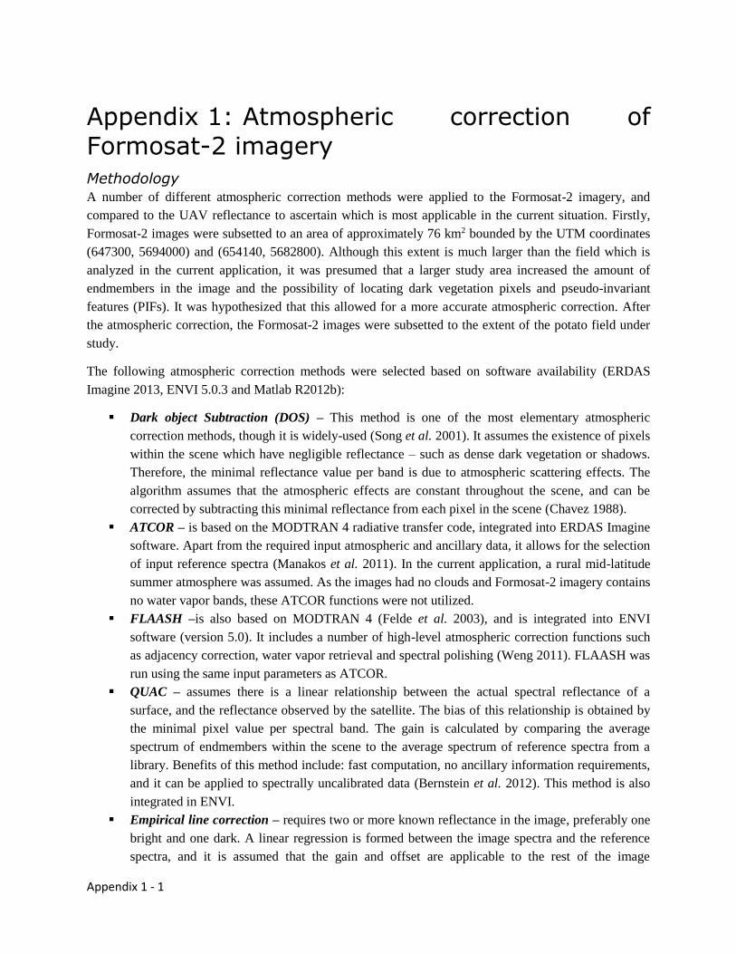
Appendix 1 - 1
Appendix 1: Atmospheric correction of
Formosat-2 imagery Methodology
A number of different atmospheric correction methods were applied to the Formosat-2 imagery, and
compared to the UAV reflectance to ascertain which is most applicable in the current situation. Firstly,
Formosat-2 images were subsetted to an area of approximately 76 km2 bounded by the UTM coordinates
(647300, 5694000) and (654140, 5682800). Although this extent is much larger than the field which is
analyzed in the current application, it was presumed that a larger study area increased the amount of
endmembers in the image and the possibility of locating dark vegetation pixels and pseudo-invariant
features (PIFs). It was hypothesized that this allowed for a more accurate atmospheric correction. After
the atmospheric correction, the Formosat-2 images were subsetted to the extent of the potato field under
study.
The following atmospheric correction methods were selected based on software availability (ERDAS
Imagine 2013, ENVI 5.0.3 and Matlab R2012b):
Dark object Subtraction (DOS) – This method is one of the most elementary atmospheric
correction methods, though it is widely-used (Song et al. 2001). It assumes the existence of pixels
within the scene which have negligible reflectance – such as dense dark vegetation or shadows.
Therefore, the minimal reflectance value per band is due to atmospheric scattering effects. The
algorithm assumes that the atmospheric effects are constant throughout the scene, and can be
corrected by subtracting this minimal reflectance from each pixel in the scene (Chavez 1988).
ATCOR – is based on the MODTRAN 4 radiative transfer code, integrated into ERDAS Imagine
software. Apart from the required input atmospheric and ancillary data, it allows for the selection
of input reference spectra (Manakos et al. 2011). In the current application, a rural mid-latitude
summer atmosphere was assumed. As the images had no clouds and Formosat-2 imagery contains
no water vapor bands, these ATCOR functions were not utilized.
FLAASH –is also based on MODTRAN 4 (Felde et al. 2003), and is integrated into ENVI
software (version 5.0). It includes a number of high-level atmospheric correction functions such
as adjacency correction, water vapor retrieval and spectral polishing (Weng 2011). FLAASH was
run using the same input parameters as ATCOR.
QUAC – assumes there is a linear relationship between the actual spectral reflectance of a
surface, and the reflectance observed by the satellite. The bias of this relationship is obtained by
the minimal pixel value per spectral band. The gain is calculated by comparing the average
spectrum of endmembers within the scene to the average spectrum of reference spectra from a
library. Benefits of this method include: fast computation, no ancillary information requirements,
and it can be applied to spectrally uncalibrated data (Bernstein et al. 2012). This method is also
integrated in ENVI.
Empirical line correction – requires two or more known reflectance in the image, preferably one
bright and one dark. A linear regression is formed between the image spectra and the reference
spectra, and it is assumed that the gain and offset are applicable to the rest of the image
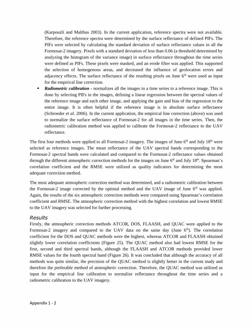
Appendix 1 - 2
(Karpouzli and Malthus 2003). In the current application, reference spectra were not available.
Therefore, the reference spectra were determined by the surface reflectance of defined PIFs. The
PIFs were selected by calculating the standard deviation of surface reflectance values in all the
Formosat-2 imagery. Pixels with a standard deviation of less than 0.06 (a threshold determined by
analyzing the histogram of the variance image) in surface reflectance throughout the time series
were defined as PIFs. These pixels were masked, and an erode filter was applied. This supported
the selection of homogenous areas, and decreased the influence of geolocation errors and
adjacency effects. The surface reflectance of the resulting pixels on June 6th were used as input
for the empirical line correction.
Radiometric calibration - normalizes all the images in a time series to a reference image. This is
done by selecting PIFs in the images, defining a linear regression between the spectral values of
the reference image and each other image, and applying the gain and bias of the regression to the
entire image. It is often helpful if the reference image is in absolute surface reflectance
(Schroeder et al. 2006). In the current application, the empirical line correction (above) was used
to normalize the surface reflectance of Formosat-2 for all images in the time series. Then, the
radiometric calibration method was applied to calibrate the Formosat-2 reflectance to the UAV
reflectance.
The first four methods were applied to all Formosat-2 imagery. The images of June 6th and July 18th were
selected as reference images. The mean reflectance of the UAV spectral bands corresponding to the
Formosat-2 spectral bands were calculated and compared to the Formosat-2 reflectance values obtained
through the different atmospheric correction methods for the images on June 6th and July 18th. Spearman’s
correlation coefficient and the RMSE were utilized as quality indicators for determining the most
adequate correction method.
The most adequate atmospheric correction method was determined, and a radiometric calibration between
the Formosat-2 image corrected by the optimal method and the UAV image of June 6th was applied.
Again, the results of the six atmospheric correction methods were compared using Spearman’s correlation
coefficient and RMSE. The atmospheric correction method with the highest correlation and lowest RMSE
to the UAV imagery was selected for further processing.
Results Firstly, the atmospheric correction methods ATCOR, DOS, FLAASH, and QUAC were applied to the
Formosat-2 imagery and compared to the UAV data on the same day (June 6th). The correlation
coefficient for the DOS and QUAC methods were the highest, whereas ATCOR and FLAASH obtained
slightly lower correlation coefficients (Figure 25). The QUAC method also had lowest RMSE for the
first, second and third spectral bands, although the FLAASH and ATCOR methods provided lower
RMSE values for the fourth spectral band (Figure 26). It was concluded that although the accuracy of all
methods was quite similar, the precision of the QUAC method is slightly better in the current study and
therefore the preferable method of atmospheric correction. Therefore, the QUAC method was utilized as
input for the empirical line calibration to normalize reflectance throughout the time series and a
radiometric calibration to the UAV imagery.
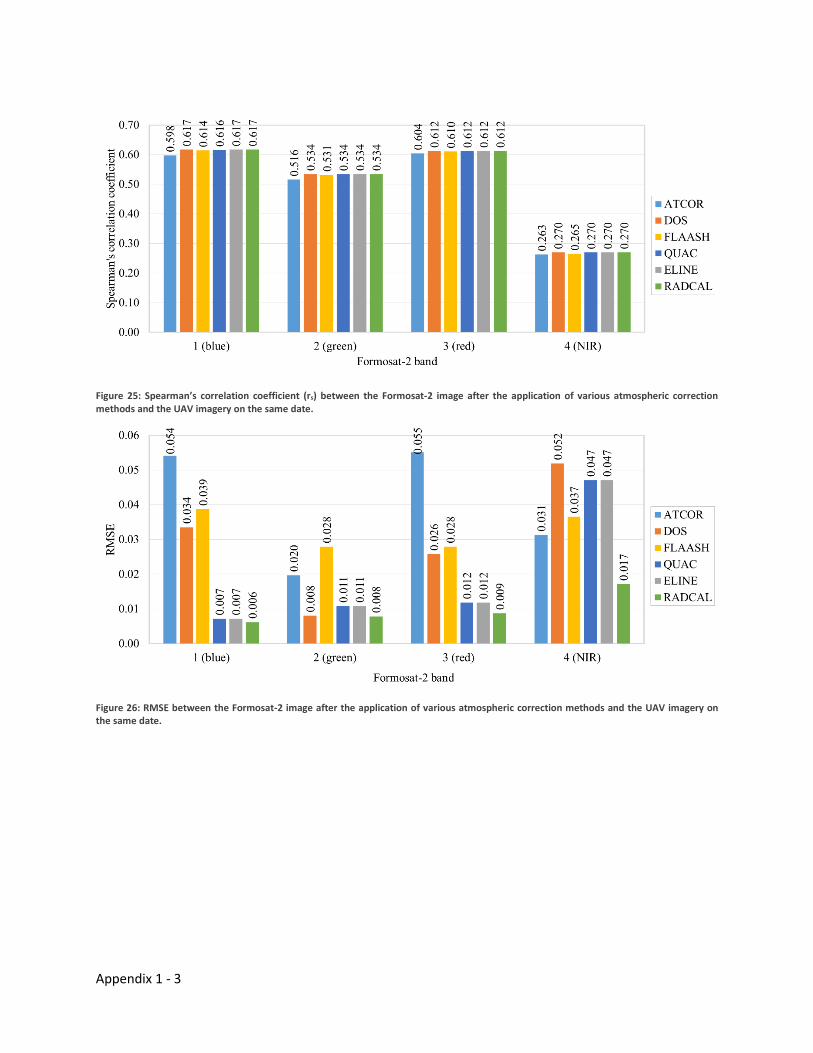
Appendix 1 - 3
Figure 25: Spearman’s correlation coefficient (rs) between the Formosat-2 image after the application of various atmospheric correction methods and the UAV imagery on the same date.
Figure 26: RMSE between the Formosat-2 image after the application of various atmospheric correction methods and the UAV imagery on the same date.
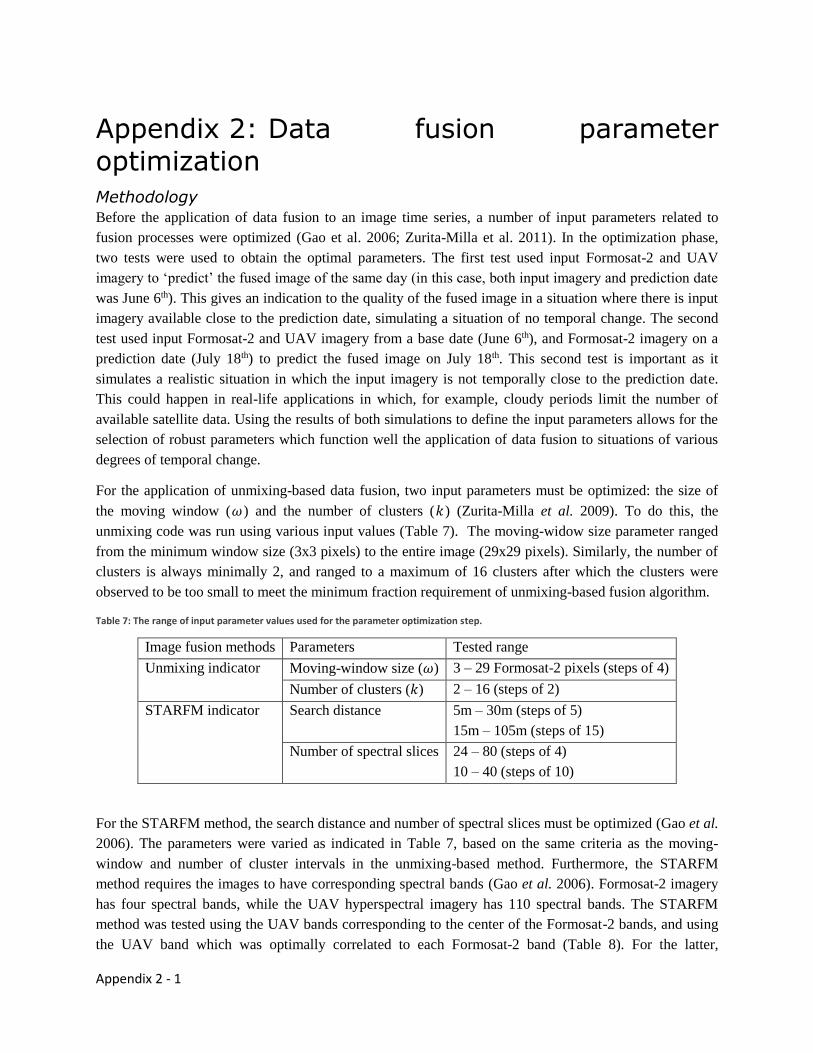
Appendix 2 - 1
Appendix 2: Data fusion parameter
optimization Methodology
Before the application of data fusion to an image time series, a number of input parameters related to
fusion processes were optimized (Gao et al. 2006; Zurita-Milla et al. 2011). In the optimization phase,
two tests were used to obtain the optimal parameters. The first test used input Formosat-2 and UAV
imagery to ‘predict’ the fused image of the same day (in this case, both input imagery and prediction date
was June 6th). This gives an indication to the quality of the fused image in a situation where there is input
imagery available close to the prediction date, simulating a situation of no temporal change. The second
test used input Formosat-2 and UAV imagery from a base date (June 6th), and Formosat-2 imagery on a
prediction date (July 18th) to predict the fused image on July 18th. This second test is important as it
simulates a realistic situation in which the input imagery is not temporally close to the prediction date.
This could happen in real-life applications in which, for example, cloudy periods limit the number of
available satellite data. Using the results of both simulations to define the input parameters allows for the
selection of robust parameters which function well the application of data fusion to situations of various
degrees of temporal change.
For the application of unmixing-based data fusion, two input parameters must be optimized: the size of
the moving window (𝜔) and the number of clusters (𝑘) (Zurita-Milla et al. 2009). To do this, the
unmixing code was run using various input values (Table 7). The moving-widow size parameter ranged
from the minimum window size (3x3 pixels) to the entire image (29x29 pixels). Similarly, the number of
clusters is always minimally 2, and ranged to a maximum of 16 clusters after which the clusters were
observed to be too small to meet the minimum fraction requirement of unmixing-based fusion algorithm.
Table 7: The range of input parameter values used for the parameter optimization step.
Image fusion methods Parameters Tested range
Unmixing indicator Moving-window size (𝜔) 3 – 29 Formosat-2 pixels (steps of 4)
Number of clusters (𝑘) 2 – 16 (steps of 2)
STARFM indicator Search distance 5m – 30m (steps of 5)
15m – 105m (steps of 15)
Number of spectral slices 24 – 80 (steps of 4)
10 – 40 (steps of 10)
For the STARFM method, the search distance and number of spectral slices must be optimized (Gao et al.
2006). The parameters were varied as indicated in Table 7, based on the same criteria as the moving-
window and number of cluster intervals in the unmixing-based method. Furthermore, the STARFM
method requires the images to have corresponding spectral bands (Gao et al. 2006). Formosat-2 imagery
has four spectral bands, while the UAV hyperspectral imagery has 110 spectral bands. The STARFM
method was tested using the UAV bands corresponding to the center of the Formosat-2 bands, and using
the UAV band which was optimally correlated to each Formosat-2 band (Table 8). For the latter,
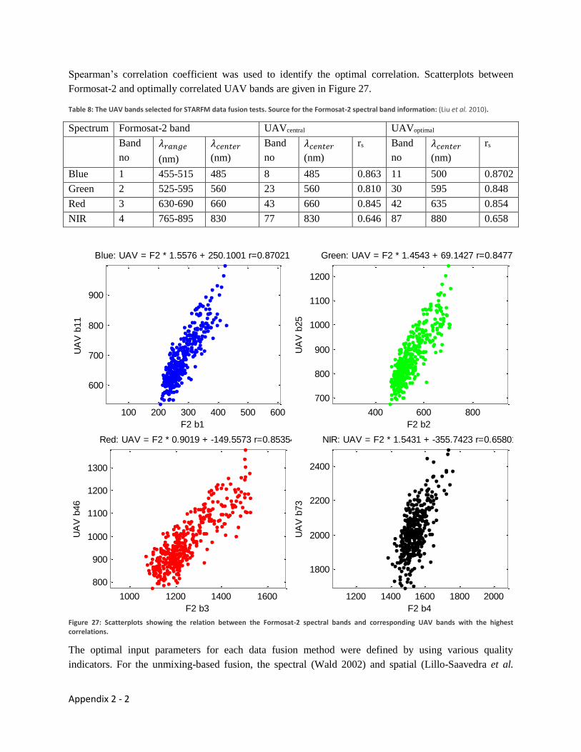
Appendix 2 - 2
Spearman’s correlation coefficient was used to identify the optimal correlation. Scatterplots between
Formosat-2 and optimally correlated UAV bands are given in Figure 27.
Table 8: The UAV bands selected for STARFM data fusion tests. Source for the Formosat-2 spectral band information: (Liu et al. 2010).
Spectrum Formosat-2 band UAVcentral UAVoptimal
Band
no
𝜆𝑟𝑎𝑛𝑔𝑒
(nm)
𝜆𝑐𝑒𝑛𝑡𝑒𝑟
(nm)
Band
no
𝜆𝑐𝑒𝑛𝑡𝑒𝑟
(nm)
rs Band
no
𝜆𝑐𝑒𝑛𝑡𝑒𝑟
(nm)
rs
Blue 1 455-515 485 8 485 0.863 11 500 0.8702
Green 2 525-595 560 23 560 0.810 30 595 0.848
Red 3 630-690 660 43 660 0.845 42 635 0.854
NIR 4 765-895 830 77 830 0.646 87 880 0.658
Figure 27: Scatterplots showing the relation between the Formosat-2 spectral bands and corresponding UAV bands with the highest correlations.
The optimal input parameters for each data fusion method were defined by using various quality
indicators. For the unmixing-based fusion, the spectral (Wald 2002) and spatial (Lillo-Saavedra et al.
100 200 300 400 500 600
600
700
800
900
Blue: UAV = F2 * 1.5576 + 250.1001 r=0.87021
UA
V b
11
F2 b1
400 600 800
700
800
900
1000
1100
1200
Green: UAV = F2 * 1.4543 + 69.1427 r=0.84777
UA
V b
25
F2 b2
1000 1200 1400 1600
800
900
1000
1100
1200
1300
Red: UAV = F2 * 0.9019 + -149.5573 r=0.85354
UA
V b
46
F2 b3
1200 1400 1600 1800 2000
1800
2000
2200
2400
NIR: UAV = F2 * 1.5431 + -355.7423 r=0.65801
UA
V b
73
F2 b4
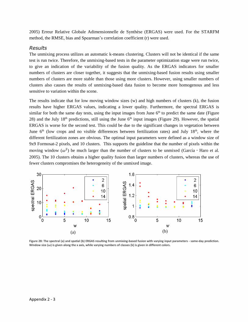
Appendix 2 - 3
2005) Erreur Relative Globale Adimensionnelle de Synthèse (ERGAS) were used. For the STARFM
method, the RMSE, bias and Spearman’s correlation coefficient (r) were used.
Results The unmixing process utilizes an automatic k-means clustering. Clusters will not be identical if the same
test is run twice. Therefore, the unmixing-based tests in the parameter optimization stage were run twice,
to give an indication of the variability of the fusion quality. As the ERGAS indicators for smaller
numbers of clusters are closer together, it suggests that the unmixing-based fusion results using smaller
numbers of clusters are more stable than those using more clusters. However, using smaller numbers of
clusters also causes the results of unmixing-based data fusion to become more homogenous and less
sensitive to variation within the scene.
The results indicate that for low moving window sizes (w) and high numbers of clusters (k), the fusion
results have higher ERGAS values, indicating a lower quality. Furthermore, the spectral ERGAS is
similar for both the same day tests, using the input images from June 6th to predict the same date (Figure
28) and the July 18th predictions, still using the June 6th input images (Figure 29). However, the spatial
ERGAS is worse for the second test. This could be due to the significant changes in vegetation between
June 6th (low crops and no visible differences between fertilization rates) and July 18th, where the
different fertilization zones are obvious. The optimal input parameters were defined as a window size of
9x9 Formosat-2 pixels, and 10 clusters. This supports the guideline that the number of pixels within the
moving window (𝜔2) be much larger than the number of clusters to be unmixed (García‐Haro et al.
2005). The 10 clusters obtains a higher quality fusion than larger numbers of clusters, whereas the use of
fewer clusters compromises the heterogeneity of the unmixed image.
(a) (b)
Figure 28: The spectral (a) and spatial (b) ERGAS resulting from unmixing-based fusion with varying input parameters - same-day prediction. Window size (𝝎) is given along the x axis, while varying numbers of classes (k) is given in different colors.
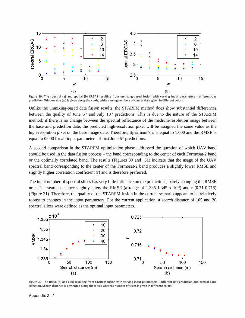
Appendix 2 - 4
(a)
(b)
Figure 29: The spectral (a) and spatial (b) ERGAS resulting from unmixing-based fusion with varying input parameters - different-day prediction. Window size (𝝎) is given along the x axis, while varying numbers of classes (k) is given in different colors.
Unlike the unmixing-based data fusion results, the STARFM method does show substantial differences
between the quality of June 6th and July 18th predictions. This is due to the nature of the STARFM
method; if there is no change between the spectral reflectance of the medium-resolution image between
the base and prediction date, the predicted high-resolution pixel will be assigned the same value as the
high-resolution pixel on the base image date. Therefore, Spearman’s rs is equal to 1.000 and the RMSE is
equal to 0.000 for all input parameters of first June 6th predictions.
A second comparison in the STARFM optimization phase addressed the question of which UAV band
should be used in the data fusion process – the band corresponding to the center of each Formosat-2 band
or the optimally correlated band. The results (Figures 30 and 31) indicate that the usage of the UAV
spectral band corresponding to the center of the Formosat-2 band produces a slightly lower RMSE and
slightly higher correlation coefficient (r) and is therefore preferred.
The input number of spectral slices has very little influence on the predictions, barely changing the RMSE
or r. The search distance slightly alters the RMSE (a range of 1.335-1.345 x 10⁻⁵) and r (0.71-0.715)
(Figure 31). Therefore, the quality of the STARFM fusion in the current scenario appears to be relatively
robust to changes in the input parameters. For the current application, a search distance of 105 and 30
spectral slices were defined as the optimal input parameters.
(a) (b)
Figure 30: The RMSE (a) and r (b) resulting from STARFM fusion with varying input parameters - different-day prediction and central band selection. Search distance is presented along the x-axis whereas number of slices is given in different colors.
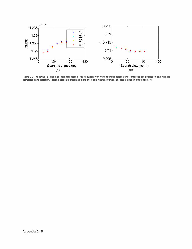
Appendix 2 - 5
(a) (b)
Figure 31: The RMSE (a) and r (b) resulting from STARFM fusion with varying input parameters - different-day prediction and highest correlated band selection. Search distance is presented along the x-axis whereas number of slices is given in different colors.
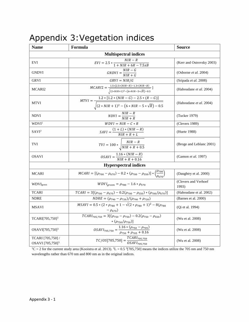
Appendix 3 - 1
Appendix 3: Vegetation indices Name Formula Source
Multispectral indices
EVI 𝐸𝑉𝐼 = 2.5 ∗𝑁𝐼𝑅 − 𝑅
1 + 𝑁𝐼𝑅 + 6𝑅 − 7.5𝑥𝐵 (Kerr and Ostrovsky 2003)
GNDVI 𝐺𝑁𝐷𝑉𝐼 =𝑁𝐼𝑅 − 𝐺
𝑁𝐼𝑅 + 𝐺 (Osborne et al. 2004)
GRVI 𝐺𝑅𝑉𝐼 = 𝑁𝐼𝑅/𝐺 (Sripada et al. 2008)
MCARI2 𝑀𝐶𝐴𝑅𝐼2 =1.5∗[2.5∗(𝑁𝐼𝑅−𝑅)−1.3∗(𝑁𝐼𝑅−𝐵)
√(2∗𝑁𝐼𝑅+1)2−(6∗𝑁𝐼𝑅−5∗√𝑅)−0.5
] (Haboudane et al. 2004)
MTVI 𝑀𝑇𝑉𝐼 =
1.2 ∗ [1.2 ∗ (𝑁𝐼𝑅 − 𝐺) − 2.5 ∗ (𝑅 − 𝐺)]
√(2 ∗ 𝑁𝐼𝑅 + 1)2 − (6 ∗ 𝑁𝐼𝑅 − 5 ∗ √𝑅) − 0.5
(Haboudane et al. 2004)
NDVI 𝑁𝐷𝑉𝐼 =𝑁𝐼𝑅 − 𝑅
𝑁𝐼𝑅 + 𝑅 (Tucker 1979)
WDVI1 𝑊𝐷𝑉𝐼 = 𝑁𝐼𝑅 − 𝐶 ∗ 𝑅 (Clevers 1989)
SAVI2 𝑆𝐴𝑉𝐼 =(1 + 𝐿) ∗ (𝑁𝐼𝑅 − 𝑅)
𝑁𝐼𝑅 + 𝑅 + 𝐿 (Huete 1988)
TVI 𝑇𝑉𝐼 = 100 ∗ √𝑁𝐼𝑅 − 𝑅
𝑁𝐼𝑅 + 𝑅 + 0.5 (Broge and Leblanc 2001)
OSAVI 𝑂𝑆𝐴𝑉𝐼 =1.16 ∗ (𝑁𝐼𝑅 − 𝑅)
𝑁𝐼𝑅 + 𝑅 + 0.16 (Gamon et al. 1997)
Hyperspectral indices
MCARI 𝑀𝐶𝐴𝑅𝐼 = [(𝜌700 − 𝜌670) − 0.2 ∗ (𝜌700 − 𝜌550)] ∗ (𝜌700
𝜌670) (Daughtry et al. 2000)
WDVIgreen 𝑊𝐷𝑉𝐼𝑔𝑟𝑒𝑒𝑛 = 𝜌780 − 1.6 ∗ 𝜌570 (Clevers and Verhoef
1993)
TCARI 𝑇𝐶𝐴𝑅𝐼 = 3[(𝜌700 − 𝜌670) − 0.2(𝜌700 − 𝜌550) ∗ (𝜌700/𝜌670)] (Haboudane et al. 2002)
NDRE 𝑁𝐷𝑅𝐸 = (𝜌790 − 𝜌720)/(𝜌790 + 𝜌720) (Barnes et al. 2000)
MSAVI 𝑀𝑆𝐴𝑉𝐼 = 0.5 ∗ (2 ∗ 𝜌780 + 1 − √(2 ∗ 𝜌780 + 1)2 − 8(𝜌780
− 𝜌670) (Qi et al. 1994)
TCARI[705,750]3 𝑇𝐶𝐴𝑅𝐼705,750 = 3[(𝜌750 − 𝜌750) − 0.2(𝜌750 − 𝜌550)
∗ (𝜌750/𝜌750)] (Wu et al. 2008)
OSAVI[705,750]3 𝑂𝑆𝐴𝑉𝐼705,750 =1.16 ∗ (𝜌750 − 𝜌705)
𝜌750 + 𝜌705 + 0.16 (Wu et al. 2008)
TCARI [705,750] /
OSAVI [705,750]3 𝑇𝐶/𝑂𝑆[705,750] =
𝑇𝐶𝐴𝑅𝐼705,750
𝑂𝑆𝐴𝑉𝐼705,750 (Wu et al. 2008)
1C = 2 for the current study area (Kooistra et al. 2013). 2L = 0.5 3[705,750] means the indices utilize the 705 nm and 750 nm
wavelengths rather than 670 nm and 800 nm as in the original indices.

Appendix 4: WHISPERS 2014 Submission
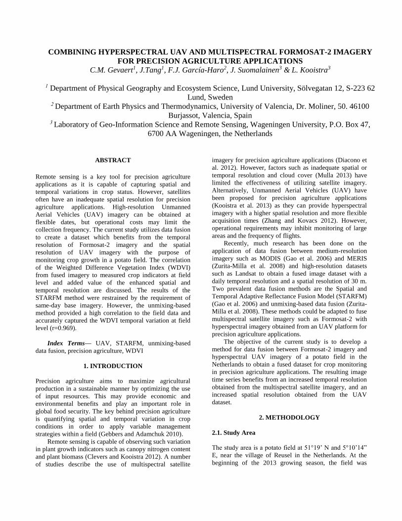
COMBINING HYPERSPECTRAL UAV AND MULTISPECTRAL FORMOSAT-2 IMAGERY
FOR PRECISION AGRICULTURE APPLICATIONS C.M. Gevaert1, J.Tang1, F.J. García-Haro2, J. Suomalainen3 & L. Kooistra3
1 Department of Physical Geography and Ecosystem Science, Lund University, Sölvegatan 12, S-223 62
Lund, Sweden 2 Department of Earth Physics and Thermodynamics, University of Valencia, Dr. Moliner, 50. 46100
Burjassot, Valencia, Spain 3 Laboratory of Geo-Information Science and Remote Sensing, Wageningen University, P.O. Box 47,
6700 AA Wageningen, the Netherlands
ABSTRACT
Remote sensing is a key tool for precision agriculture
applications as it is capable of capturing spatial and
temporal variations in crop status. However, satellites
often have an inadequate spatial resolution for precision
agriculture applications. High-resolution Unmanned
Aerial Vehicles (UAV) imagery can be obtained at
flexible dates, but operational costs may limit the
collection frequency. The current study utilizes data fusion
to create a dataset which benefits from the temporal
resolution of Formosat-2 imagery and the spatial
resolution of UAV imagery with the purpose of
monitoring crop growth in a potato field. The correlation
of the Weighted Difference Vegetation Index (WDVI)
from fused imagery to measured crop indicators at field
level and added value of the enhanced spatial and
temporal resolution are discussed. The results of the
STARFM method were restrained by the requirement of
same-day base imagery. However, the unmixing-based
method provided a high correlation to the field data and
accurately captured the WDVI temporal variation at field
level (r=0.969).
Index Terms— UAV, STARFM, unmixing-based
data fusion, precision agriculture, WDVI
1. INTRODUCTION
Precision agriculture aims to maximize agricultural
production in a sustainable manner by optimizing the use
of input resources. This may provide economic and
environmental benefits and play an important role in
global food security. The key behind precision agriculture
is quantifying spatial and temporal variation in crop
conditions in order to apply variable management
strategies within a field (Gebbers and Adamchuk 2010).
Remote sensing is capable of observing such variation
in plant growth indicators such as canopy nitrogen content
and plant biomass (Clevers and Kooistra 2012). A number
of studies describe the use of multispectral satellite
imagery for precision agriculture applications (Diacono et
al. 2012). However, factors such as inadequate spatial or
temporal resolution and cloud cover (Mulla 2013) have
limited the effectiveness of utilizing satellite imagery.
Alternatively, Unmanned Aerial Vehicles (UAV) have
been proposed for precision agriculture applications
(Kooistra et al. 2013) as they can provide hyperspectral
imagery with a higher spatial resolution and more flexible
acquisition times (Zhang and Kovacs 2012). However,
operational requirements may inhibit monitoring of large
areas and the frequency of flights.
Recently, much research has been done on the
application of data fusion between medium-resolution
imagery such as MODIS (Gao et al. 2006) and MERIS
(Zurita-Milla et al. 2008) and high-resolution datasets
such as Landsat to obtain a fused image dataset with a
daily temporal resolution and a spatial resolution of 30 m.
Two prevalent data fusion methods are the Spatial and
Temporal Adaptive Reflectance Fusion Model (STARFM)
(Gao et al. 2006) and unmixing-based data fusion (Zurita-
Milla et al. 2008). These methods could be adapted to fuse
multispectral satellite imagery such as Formosat-2 with
hyperspectral imagery obtained from an UAV platform for
precision agriculture applications.
The objective of the current study is to develop a
method for data fusion between Formosat-2 imagery and
hyperspectral UAV imagery of a potato field in the
Netherlands to obtain a fused dataset for crop monitoring
in precision agriculture applications. The resulting image
time series benefits from an increased temporal resolution
obtained from the multispectral satellite imagery, and an
increased spatial resolution obtained from the UAV
dataset.
2. METHODOLOGY
2.1. Study Area
The study area is a potato field at 51°19’ N and 5°10’14”
E, near the village of Reusel in the Netherlands. At the
beginning of the 2013 growing season, the field was
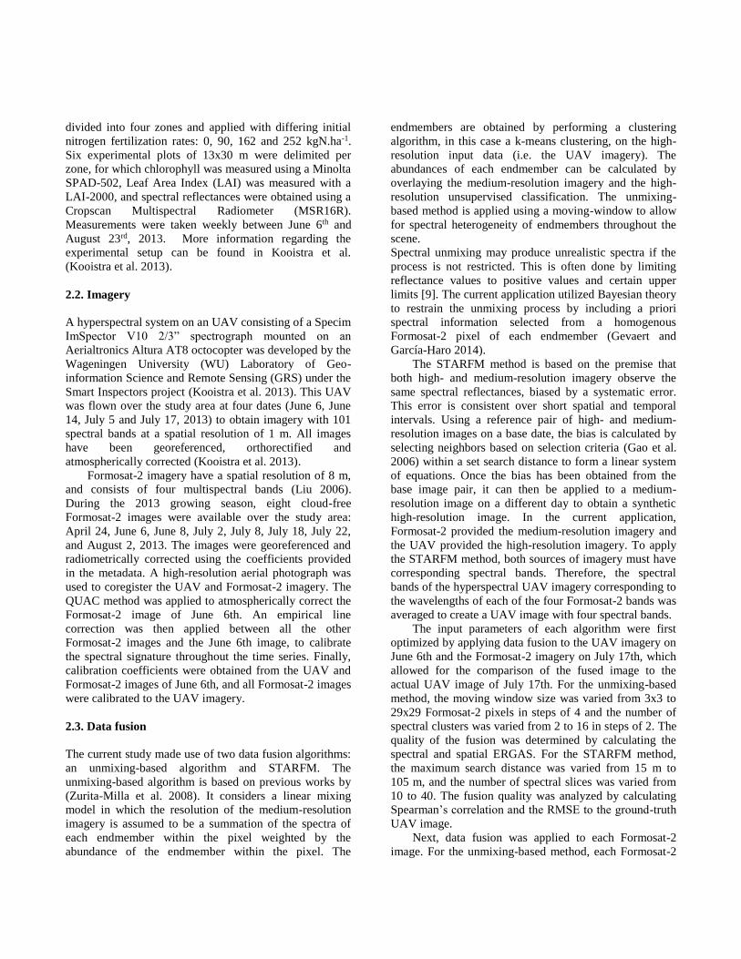
divided into four zones and applied with differing initial
nitrogen fertilization rates: 0, 90, 162 and 252 kgN.ha-1.
Six experimental plots of 13x30 m were delimited per
zone, for which chlorophyll was measured using a Minolta
SPAD-502, Leaf Area Index (LAI) was measured with a
LAI-2000, and spectral reflectances were obtained using a
Cropscan Multispectral Radiometer (MSR16R).
Measurements were taken weekly between June 6th and
August 23rd, 2013. More information regarding the
experimental setup can be found in Kooistra et al.
(Kooistra et al. 2013).
2.2. Imagery
A hyperspectral system on an UAV consisting of a Specim
ImSpector V10 2/3” spectrograph mounted on an
Aerialtronics Altura AT8 octocopter was developed by the
Wageningen University (WU) Laboratory of Geo-
information Science and Remote Sensing (GRS) under the
Smart Inspectors project (Kooistra et al. 2013). This UAV
was flown over the study area at four dates (June 6, June
14, July 5 and July 17, 2013) to obtain imagery with 101
spectral bands at a spatial resolution of 1 m. All images
have been georeferenced, orthorectified and
atmospherically corrected (Kooistra et al. 2013).
Formosat-2 imagery have a spatial resolution of 8 m,
and consists of four multispectral bands (Liu 2006).
During the 2013 growing season, eight cloud-free
Formosat-2 images were available over the study area:
April 24, June 6, June 8, July 2, July 8, July 18, July 22,
and August 2, 2013. The images were georeferenced and
radiometrically corrected using the coefficients provided
in the metadata. A high-resolution aerial photograph was
used to coregister the UAV and Formosat-2 imagery. The
QUAC method was applied to atmospherically correct the
Formosat-2 image of June 6th. An empirical line
correction was then applied between all the other
Formosat-2 images and the June 6th image, to calibrate
the spectral signature throughout the time series. Finally,
calibration coefficients were obtained from the UAV and
Formosat-2 images of June 6th, and all Formosat-2 images
were calibrated to the UAV imagery.
2.3. Data fusion
The current study made use of two data fusion algorithms:
an unmixing-based algorithm and STARFM. The
unmixing-based algorithm is based on previous works by
(Zurita-Milla et al. 2008). It considers a linear mixing
model in which the resolution of the medium-resolution
imagery is assumed to be a summation of the spectra of
each endmember within the pixel weighted by the
abundance of the endmember within the pixel. The
endmembers are obtained by performing a clustering
algorithm, in this case a k-means clustering, on the high-
resolution input data (i.e. the UAV imagery). The
abundances of each endmember can be calculated by
overlaying the medium-resolution imagery and the high-
resolution unsupervised classification. The unmixing-
based method is applied using a moving-window to allow
for spectral heterogeneity of endmembers throughout the
scene.
Spectral unmixing may produce unrealistic spectra if the
process is not restricted. This is often done by limiting
reflectance values to positive values and certain upper
limits [9]. The current application utilized Bayesian theory
to restrain the unmixing process by including a priori
spectral information selected from a homogenous
Formosat-2 pixel of each endmember (Gevaert and
García-Haro 2014).
The STARFM method is based on the premise that
both high- and medium-resolution imagery observe the
same spectral reflectances, biased by a systematic error.
This error is consistent over short spatial and temporal
intervals. Using a reference pair of high- and medium-
resolution images on a base date, the bias is calculated by
selecting neighbors based on selection criteria (Gao et al.
2006) within a set search distance to form a linear system
of equations. Once the bias has been obtained from the
base image pair, it can then be applied to a medium-
resolution image on a different day to obtain a synthetic
high-resolution image. In the current application,
Formosat-2 provided the medium-resolution imagery and
the UAV provided the high-resolution imagery. To apply
the STARFM method, both sources of imagery must have
corresponding spectral bands. Therefore, the spectral
bands of the hyperspectral UAV imagery corresponding to
the wavelengths of each of the four Formosat-2 bands was
averaged to create a UAV image with four spectral bands.
The input parameters of each algorithm were first
optimized by applying data fusion to the UAV imagery on
June 6th and the Formosat-2 imagery on July 17th, which
allowed for the comparison of the fused image to the
actual UAV image of July 17th. For the unmixing-based
method, the moving window size was varied from 3x3 to
29x29 Formosat-2 pixels in steps of 4 and the number of
spectral clusters was varied from 2 to 16 in steps of 2. The
quality of the fusion was determined by calculating the
spectral and spatial ERGAS. For the STARFM method,
the maximum search distance was varied from 15 m to
105 m, and the number of spectral slices was varied from
10 to 40. The fusion quality was analyzed by calculating
Spearman’s correlation and the RMSE to the ground-truth
UAV image.
Next, data fusion was applied to each Formosat-2
image. For the unmixing-based method, each Formosat-2
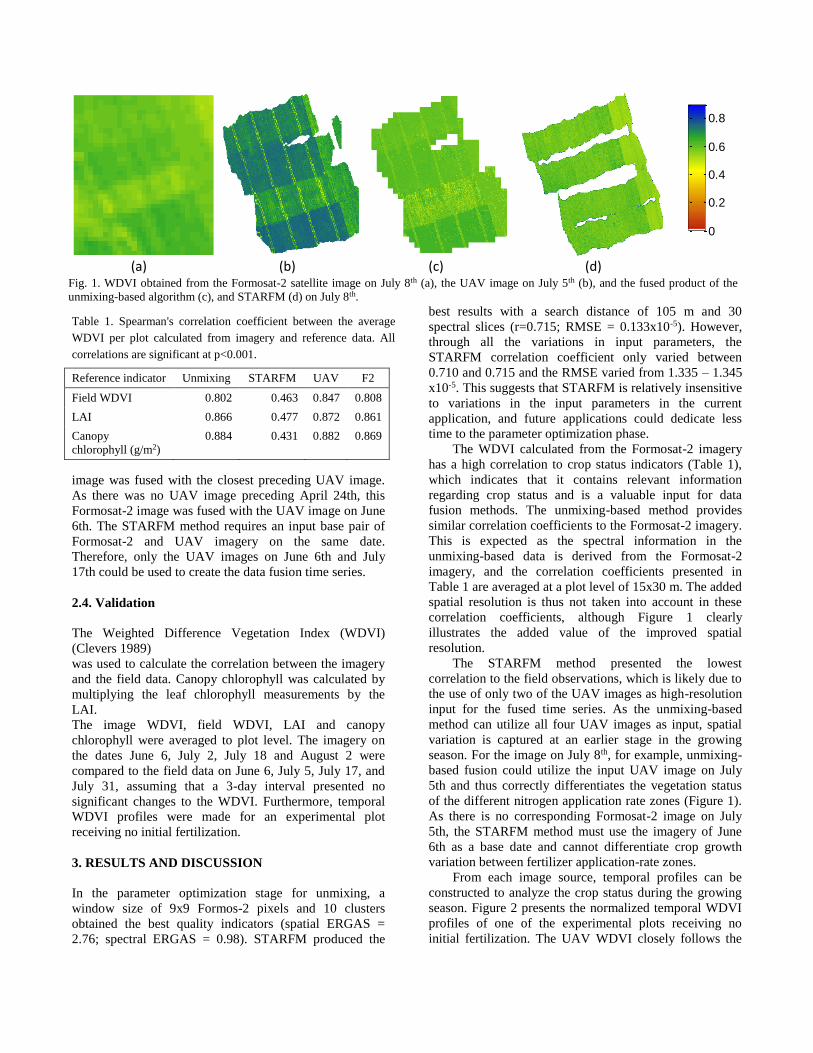
image was fused with the closest preceding UAV image.
As there was no UAV image preceding April 24th, this
Formosat-2 image was fused with the UAV image on June
6th. The STARFM method requires an input base pair of
Formosat-2 and UAV imagery on the same date.
Therefore, only the UAV images on June 6th and July
17th could be used to create the data fusion time series.
2.4. Validation
The Weighted Difference Vegetation Index (WDVI)
(Clevers 1989)
was used to calculate the correlation between the imagery
and the field data. Canopy chlorophyll was calculated by
multiplying the leaf chlorophyll measurements by the
LAI. The image WDVI, field WDVI, LAI and canopy
chlorophyll were averaged to plot level. The imagery on
the dates June 6, July 2, July 18 and August 2 were
compared to the field data on June 6, July 5, July 17, and
July 31, assuming that a 3-day interval presented no
significant changes to the WDVI. Furthermore, temporal
WDVI profiles were made for an experimental plot
receiving no initial fertilization.
3. RESULTS AND DISCUSSION
In the parameter optimization stage for unmixing, a
window size of 9x9 Formos-2 pixels and 10 clusters
obtained the best quality indicators (spatial ERGAS =
2.76; spectral ERGAS = 0.98). STARFM produced the
best results with a search distance of 105 m and 30
spectral slices (r=0.715; RMSE = 0.133x10⁻⁵). However,
through all the variations in input parameters, the
STARFM correlation coefficient only varied between
0.710 and 0.715 and the RMSE varied from 1.335 – 1.345
x10-5. This suggests that STARFM is relatively insensitive
to variations in the input parameters in the current
application, and future applications could dedicate less
time to the parameter optimization phase.
The WDVI calculated from the Formosat-2 imagery
has a high correlation to crop status indicators (Table 1),
which indicates that it contains relevant information
regarding crop status and is a valuable input for data
fusion methods. The unmixing-based method provides
similar correlation coefficients to the Formosat-2 imagery.
This is expected as the spectral information in the
unmixing-based data is derived from the Formosat-2
imagery, and the correlation coefficients presented in
Table 1 are averaged at a plot level of 15x30 m. The added
spatial resolution is thus not taken into account in these
correlation coefficients, although Figure 1 clearly
illustrates the added value of the improved spatial
resolution.
The STARFM method presented the lowest
correlation to the field observations, which is likely due to
the use of only two of the UAV images as high-resolution
input for the fused time series. As the unmixing-based
method can utilize all four UAV images as input, spatial
variation is captured at an earlier stage in the growing
season. For the image on July 8th, for example, unmixing-
based fusion could utilize the input UAV image on July
5th and thus correctly differentiates the vegetation status
of the different nitrogen application rate zones (Figure 1).
As there is no corresponding Formosat-2 image on July
5th, the STARFM method must use the imagery of June
6th as a base date and cannot differentiate crop growth
variation between fertilizer application-rate zones.
From each image source, temporal profiles can be
constructed to analyze the crop status during the growing
season. Figure 2 presents the normalized temporal WDVI
profiles of one of the experimental plots receiving no
initial fertilization. The UAV WDVI closely follows the
Reference indicator Unmixing STARFM UAV F2
Field WDVI 0.802 0.463 0.847 0.808
LAI 0.866 0.477 0.872 0.861
Canopy
chlorophyll (g/m2)
0.884 0.431 0.882 0.869
(a)
(b)
(c)
(d)
Fig. 1. WDVI obtained from the Formosat-2 satellite image on July 8th (a), the UAV image on July 5th (b), and the fused product of the
unmixing-based algorithm (c), and STARFM (d) on July 8th.
0
0.2
0.4
0.6
0.8
Table 1. Spearman's correlation coefficient between the average
WDVI per plot calculated from imagery and reference data. All
correlations are significant at p<0.001.
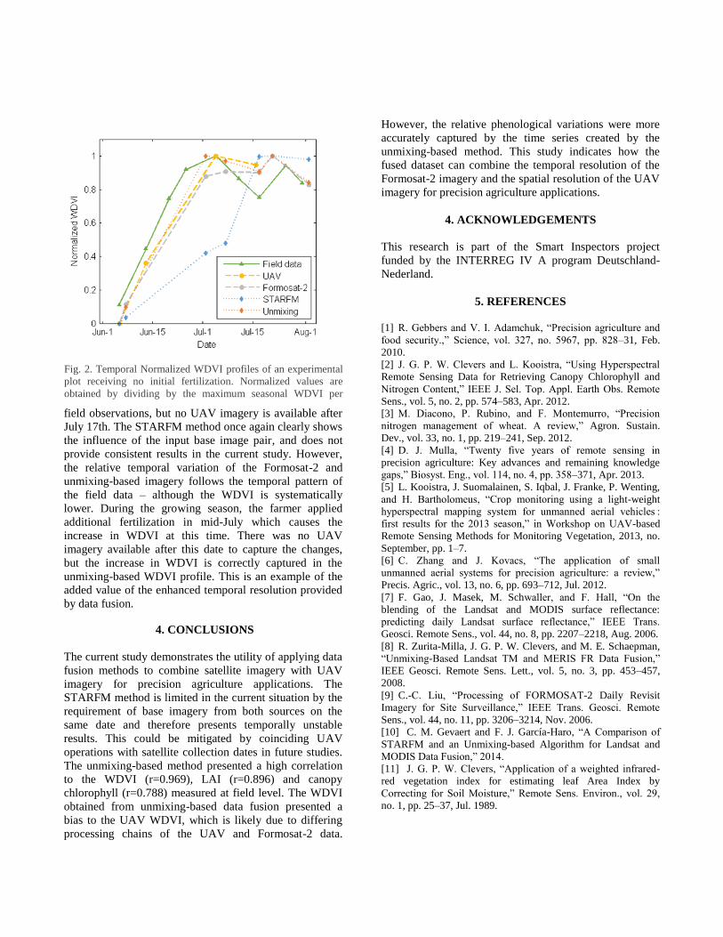
field observations, but no UAV imagery is available after
July 17th. The STARFM method once again clearly shows
the influence of the input base image pair, and does not
provide consistent results in the current study. However,
the relative temporal variation of the Formosat-2 and
unmixing-based imagery follows the temporal pattern of
the field data – although the WDVI is systematically
lower. During the growing season, the farmer applied
additional fertilization in mid-July which causes the
increase in WDVI at this time. There was no UAV
imagery available after this date to capture the changes,
but the increase in WDVI is correctly captured in the
unmixing-based WDVI profile. This is an example of the
added value of the enhanced temporal resolution provided
by data fusion.
4. CONCLUSIONS
The current study demonstrates the utility of applying data
fusion methods to combine satellite imagery with UAV
imagery for precision agriculture applications. The
STARFM method is limited in the current situation by the
requirement of base imagery from both sources on the
same date and therefore presents temporally unstable
results. This could be mitigated by coinciding UAV
operations with satellite collection dates in future studies.
The unmixing-based method presented a high correlation
to the WDVI (r=0.969), LAI (r=0.896) and canopy
chlorophyll (r=0.788) measured at field level. The WDVI
obtained from unmixing-based data fusion presented a
bias to the UAV WDVI, which is likely due to differing
processing chains of the UAV and Formosat-2 data.
However, the relative phenological variations were more
accurately captured by the time series created by the
unmixing-based method. This study indicates how the
fused dataset can combine the temporal resolution of the
Formosat-2 imagery and the spatial resolution of the UAV
imagery for precision agriculture applications.
4. ACKNOWLEDGEMENTS
This research is part of the Smart Inspectors project
funded by the INTERREG IV A program Deutschland-
Nederland.
5. REFERENCES
[1] R. Gebbers and V. I. Adamchuk, “Precision agriculture and
food security.,” Science, vol. 327, no. 5967, pp. 828–31, Feb.
2010.
[2] J. G. P. W. Clevers and L. Kooistra, “Using Hyperspectral
Remote Sensing Data for Retrieving Canopy Chlorophyll and
Nitrogen Content,” IEEE J. Sel. Top. Appl. Earth Obs. Remote
Sens., vol. 5, no. 2, pp. 574–583, Apr. 2012.
[3] M. Diacono, P. Rubino, and F. Montemurro, “Precision
nitrogen management of wheat. A review,” Agron. Sustain.
Dev., vol. 33, no. 1, pp. 219–241, Sep. 2012.
[4] D. J. Mulla, “Twenty five years of remote sensing in
precision agriculture: Key advances and remaining knowledge
gaps,” Biosyst. Eng., vol. 114, no. 4, pp. 358–371, Apr. 2013.
[5] L. Kooistra, J. Suomalainen, S. Iqbal, J. Franke, P. Wenting,
and H. Bartholomeus, “Crop monitoring using a light-weight
hyperspectral mapping system for unmanned aerial vehicles :
first results for the 2013 season,” in Workshop on UAV-based
Remote Sensing Methods for Monitoring Vegetation, 2013, no.
September, pp. 1–7.
[6] C. Zhang and J. Kovacs, “The application of small
unmanned aerial systems for precision agriculture: a review,”
Precis. Agric., vol. 13, no. 6, pp. 693–712, Jul. 2012.
[7] F. Gao, J. Masek, M. Schwaller, and F. Hall, “On the
blending of the Landsat and MODIS surface reflectance:
predicting daily Landsat surface reflectance,” IEEE Trans.
Geosci. Remote Sens., vol. 44, no. 8, pp. 2207–2218, Aug. 2006.
[8] R. Zurita-Milla, J. G. P. W. Clevers, and M. E. Schaepman,
“Unmixing-Based Landsat TM and MERIS FR Data Fusion,”
IEEE Geosci. Remote Sens. Lett., vol. 5, no. 3, pp. 453–457,
2008.
[9] C.-C. Liu, “Processing of FORMOSAT-2 Daily Revisit
Imagery for Site Surveillance,” IEEE Trans. Geosci. Remote
Sens., vol. 44, no. 11, pp. 3206–3214, Nov. 2006.
[10] C. M. Gevaert and F. J. García-Haro, “A Comparison of
STARFM and an Unmixing-based Algorithm for Landsat and
MODIS Data Fusion,” 2014.
[11] J. G. P. W. Clevers, “Application of a weighted infrared-
red vegetation index for estimating leaf Area Index by
Correcting for Soil Moisture,” Remote Sens. Environ., vol. 29,
no. 1, pp. 25–37, Jul. 1989.
Fig. 2. Temporal Normalized WDVI profiles of an experimental
plot receiving no initial fertilization. Normalized values are
obtained by dividing by the maximum seasonal WDVI per dataset.