community phylogenetics at the biogeographical scale: cold tolerance, niche ... phylogenetics at...

SPECIALPAPER

Community phylogenetics at thebiogeographical scale: cold tolerance,niche conservatism and the structureof North American forestsBradford A. Hawkins1*, Marta Rueda1, Thiago F. Rangel2, Richard Field3

and Jos�e Alexandre F. Diniz-Filho2

1Department of Ecology & Evolutionary

Biology, University of California, Irvine,

California, USA, 2Departamento de Ecologia,

ICB, Universidade Federal de Goi�as, Goiania,

Goi�as, Brazil, 3School of Geography,

University of Nottingham, Nottingham, UK

*Correspondence: Bradford A. Hawkins,

Department of Ecology & Evolutionary

Biology, University of California, Irvine, CA

92697, USA.

E-mail: [email protected]

This is an open access article under the terms

of the Creative Commons Attribution License,

which permits use, distribution and

reproduction in any medium, provided the

original work is properly cited.

ABSTRACT

Aim The fossil record has led to a historical explanation for forest diversity

gradients within the cool parts of the Northern Hemisphere, founded on a lim-

ited ability of woody angiosperm clades to adapt to mid-Tertiary cooling. We

tested four predictions of how this should be manifested in the phylogenetic

structure of 91,340 communities: (1) forests to the north should comprise spe-

cies from younger clades (families) than forests to the south; (2) average cold

tolerance at a local site should be associated with the mean family age (MFA)

of species; (3) minimum temperature should account for MFA better than

alternative environmental variables; and (4) traits associated with survival in

cold climates should evolve under a niche conservatism constraint.

Location The contiguous United States.

Methods We extracted angiosperms from the US Forest Service’s Forest

Inventory and Analysis database. MFA was calculated by assigning age of the

family to which each species belongs and averaging across the species in each

community. We developed a phylogeny to identify phylogenetic signal in five

traits: realized cold tolerance, seed size, seed dispersal mode, leaf phenology

and height. Phylogenetic signal representation curves and phylogenetic general-

ized least squares were used to compare patterns of trait evolution against

Brownian motion. Eleven predictors structured at broad or local scales were

generated to explore relationships between environment and MFA using

random forest and general linear models.

Results Consistent with predictions, (1) southern communities comprise

angiosperm species from older families than northern communities, (2) cold

tolerance is the trait most strongly associated with local MFA, (3) minimum

temperature in the coldest month is the environmental variable that best

describes MFA, broad-scale variables being much stronger correlates than local-

scale variables, and (4) the phylogenetic structures of cold tolerance and at

least one other trait associated with survivorship in cold climates indicate niche

conservatism.

Main conclusions Tropical niche conservatism in the face of long-term cli-

mate change, probably initiated in the Late Cretaceous associated with the rise

of the Rocky Mountains, is a strong driver of the phylogenetic structure of the

angiosperm component of forest communities across the USA. However, local

deterministic and/or stochastic processes account for perhaps a quarter of the

variation in the MFA of local communities.

Keywords

Forest phylogenetics, National Forest Inventory, niche conservatism, North

America, phylogenetic signal representation, random forests, trait evolution,

tree communities, tropical conservatism hypothesis.

ª 2013 John Wiley & Sons Ltd http://wileyonlinelibrary.com/journal/jbi 1doi:10.1111/jbi.12171

Journal of Biogeography (J. Biogeogr.) (2013)

INTRODUCTION

At the biogeographical scale the evolution of cold tolerance

represents a key innovation that has permitted many tree

clades to persist in high northern latitudes after the global

cooling initiated at the end of the Eocene (Latham & Ricklefs,

1993; Ricklefs, 2005; Donoghue, 2008). The fossil record for

North American, Asian and European trees is broadly consis-

tent with this (Hsu, 1983; Latham & Ricklefs, 1993; Graham,

1999; Ricklefs, 2005), woody clades have undergone relatively

slow rates of climatic niche evolution over long periods of

time (Smith & Beaulieu, 2009), and angiosperm families

comprising trees become progressively younger on average

moving from the equator northwards (Hawkins et al., 2011)

– a phylogenetically structured spatial pattern measured by

mean family age. Thus, multiple lines of evidence indicate

that for angiosperms at least, geographical patterns of tree

diversity are consistent with the tropical conservatism

hypothesis (Wiens & Donoghue, 2004). Under that hypothe-

sis phylogenetic niche conservatism (PNC) of ancestral traits

associated with tropical conditions has largely driven the phy-

logenetic structure and composition of regional species pools,

where minimum temperatures to which regions are exposed

determine which clades are able to persist in them. And

although niche evolution has obviously occurred in multiple

tree clades throughout their history, the evolution of cold tol-

erance among trees has been difficult and has come at a cost,

with a trade-off between freezing tolerance and growth rates

in warm climates (Koehler et al., 2012).

Local communities are necessarily assembled from regional

species pools: if we can assume that cold tolerance is the pri-

mary determinant of which clades of trees occur in different

parts of North America and that niche conservatism in trees

is strong and manifested at the family rank, then we can pre-

dict that the continental-scale pattern of family age structure

will be apparent at the local scale. (See Latham & Ricklefs,

1993, for fossil-based evidence that cold tolerance is con-

served at the family rank and that entire tree families have

responded to mid-Tertiary climate change.) That is, local

forest communities will comprise species from older families

carrying the ancestral trait (intolerance to freezing) in war-

mer climates and species from younger families carrying the

derived trait (freezing tolerance) in colder climates (predic-

tion 1). This should be true above and beyond any other

influences on community composition. Second, although

many traits influence the assembly of forest communities

and facilitate species coexistence (see e.g. Swenson & Weiser,

2010; Koehler et al., 2012; Kunstler et al., 2012; Lines et al.,

2012; Swenson et al., 2012; Drescher & Thomas, 2013), cold

tolerance should be strongly associated with the mean family

age of local communities relative to other traits (prediction

2). Third, minimum temperatures to which local communi-

ties are exposed should be the primary environmental corre-

late of mean family age in local communities of angiosperm

species (prediction 3), even if other climatic influences on

trees also exist (Sakai & Weiser, 1973).

An important aspect of evaluations of tropical niche con-

servatism as an explanation for tree phylogenetic composi-

tion at either biogeographical or local scales is the

assumption that cold tolerance is phylogenetically con-

served. The fossil record provides evidence that cold toler-

ance contains phylogenetic signal (see e.g. Latham &

Ricklefs, 1993), but by some definitions that is not suffi-

cient to assume PNC, which Losos (2008, p. 996) defines

as ‘the phenomenon that closely related species are more

ecologically similar than might be expected solely as a

Brownian motion evolution’. Although strong PNC can also

result in an apparent lack of phylogenetic signal (Wiens

et al., 2010), and for other workers Brownian motion evo-

lution is sufficient to define PNC, it remains that phyloge-

netic conservatism of traits of interest must exist if it is to

be invoked as an explanation for observed patterns,

whether for cold tolerance or any other presumed key trait

(prediction 4). We agree with Losos (2008) that PNC

should be demonstrated empirically, if possible, irrespective

of disagreements about whether a Brownian motion model

of trait evolution is sufficient or not (see also Cooper et al.,

2010, for discussion of alternative macroevolutionary mod-

els underlying PNC).

In this study we tested the four predictions using two

sets of analyses: (1) geographical analysis of local commu-

nity data from the US Forest Service’s Forest Inventory and

Analysis (FIA) database; and (2) macroevolutionary analyses

of trait evolution. Using the spatial FIA data set, we docu-

mented the geographical pattern of mean family age (MFA)

of angiosperm communities to test whether the biogeo-

graphical pattern of decreasing family age to the north

identified by Hawkins et al. (2011) generates a similar pat-

tern at the local scale (prediction 1). This is the metric of

phylogenetic structure that we attempt to understand,

because it provides a core measure of tropical niche conser-

vatism for North American trees (Latham & Ricklefs, 1993).

This metric differs from the phylogenetic dispersion metrics

normally associated with the field of ‘community phyloge-

netics’, but we feel that the field can be broadened to

include other aspects of phylogenetically structured commu-

nity composition, especially linking traits to patterns of

community composition analysed in an explicit phyloge-

netic framework.

Our macroevolutionary analyses were of five traits for

which we could obtain information for at least 60% of spe-

cies and which we felt could be physiologically linked to

mean family age, including an estimate of cold tolerance,

seed size, dispersal mode, leaf phenology and height, to test

for PNC (prediction 4). Using the FIA data, we then evalu-

ated the relationships between mean trait values in local

communities and MFA to identify the traits most strongly

associated with phylogenetic structure (i.e. MFA) (predic-

tion 2). Finally, we examined 11 environmental variables

operating at broad and/or local scales to determine whether

minimum winter temperature best explains statistically the

geographical pattern of MFA in the FIA data (prediction

Journal of Biogeographyª 2013 John Wiley & Sons Ltd

2

B. A. Hawkins et al.

3). It was not our goal to identify all of the local and

regional influences on community structure, although local

communities are influenced by both (e.g. White & Hurl-

bert, 2010; Lessard et al., 2012). Rather, we evaluated the

extent to which cold tolerance and other traits that facili-

tate survivorship in cold climates are phylogenetically con-

served, and the extent to which tropical niche conservatism

can account for the age structure of local arboreal angio-

sperm communities.

MATERIALS AND METHODS

Forest community data

The community data comprise 91,340 plots, each of 0.07

hectares, in the contiguous USA extracted from the US For-

est Service’s Forest Inventory and Analysis (FIA) database

(http://www.fia.fs.fed.us/, accessed in January, 2012). For

inclusion, a site had to support at least two angiosperm tree

species and be coded as a ‘natural stand’. All gymnosperms

were removed from the data because they have very different

evolutionary histories from angiosperms (Graham, 1999).

Sites from Alaska were also excluded because they are

primarily or exclusively composed of gymnosperms.

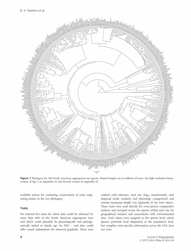
Tree phylogeny

The phylogeny used to examine trait evolution was based on

APG III (Angiosperm Phylogeny Group, 2009), to which we

added lower taxonomic ranks using the mega-phylogeny of

Smith et al. (2011) (available at http://datadryad.org/

resource/doi:10.5061/dryad.8790) and group-specific phyloge-

nies available in the primary literature (Appendix S1 in Sup-

porting Information). All species of angiosperms were

included in the phylogeny, whether sampled or not by the

FIA (Fig. 1; high resolution linear version in Appendix S2

and Newick version in Appendix S1). The definition of trees

was that of Elias (1980), which includes some groups and

species not universally considered to be trees (e.g. some yuc-

cas and cacti), and we included all currently recognized spe-

cies native to North America north of Mexico, irrespective of

whether or not they were sampled by the FIA. Infra-familial

tree structure was based on the most highly resolved group-

specific phylogenies we were able to locate. When it was not

possible to determine the most likely phylogenetic relation-

ships, judging by the conclusions of the original authors or

inconsistencies between genes or studies, we treated the rele-

vant taxa as polytomies. No branch lengths were included.

Species not resolved or not included in the phylogenies were

treated as basal polytomies. We calibrated the phylogeny by

dating nodes with the branch length adjustment function

(BLADJ) in phylocom (Webb et al., 2008), using 74 nodes

in our phylogeny matched against the dated phylogeny of

Bell et al. (2010), which represents the most complete source

for node ages of angiosperms although many of their family

age estimates are less accurate than alternative sources of

information (see next section). BLADJ assigns undated nodes

equal branch lengths between nodes for which age estimates

are available.

Mean family age (MFA)

We used two estimates of family crown ages to generate

MFA. First, we use the molecular-based ages provided by

Davies et al. (2004). MFA was calculated by assigning all spe-

cies the age of the family to which they belong (see Appen-

dix S3) and then averaging across all species occurring at

each site. We used Davies et al. (2004) rather than Bell et al.

(2010) for the geographical analysis because a comparison of

their estimates against fossil-based age estimates for the fami-

lies sampled by the FIA indicated that the ages in Davies

et al. (2004) more closely matched the fossil record than did

the ages of Bell et al. (2010) (Appendix S3), suggesting that

there are some potential problems with the age estimates in

the later study. Because we were able to obtain fossil-based

minimum ages for all but three families (comprising 10 spe-

cies) sampled by the FIA, we also generated MFA based on

these ages, using mid-points when age estimates were

bounded or minimum age + 1 Myr when only minimum

bounds were known. This allowed us to evaluate the robust-

ness of the MFA pattern with respect to source of the age

estimates, although we used the more complete and arguably

more precise data from Davies et al. (2004) for analytical

purposes.

The use of family to assign ages assumes that there is

strong conservation of traits relevant to geographical distri-

butions at the family rank, an assumption for which there is

fossil-based support (Latham & Ricklefs, 1993). It also

ignores intra-familial variation in traits, which if extensive

could obscure broader patterns originating from patterns of

trait evolution deep in the history of angiosperms. Like all

taxonomic ranks above species, family designations contain

arbitrary components, but using distribution maps for fami-

lies and their ages Hawkins et al. (2011) found a strong lati-

tudinal gradient of mean age of arboreal families in North

America consistent with a tropical conservatism prediction.

This indicates that interpretable evolutionary signal is con-

tained at the family level, at least for arborescent angio-

sperms. Calculating MFA also permits a direct comparison

of the local patterns generated at the species level with that

found by Hawkins et al. (2011) using range maps of families

and a global grid system. It is also important to realize that

ages of lower ranks (particularly species) are not appropriate

for the type of analysis we are conducting, for two reasons.

First, species ages depend on diversification rates more than

niche conservatism and thus address a different mechanism.

Second, ages of lower taxonomic ranks are expected to be

more biased by extinctions than higher ranks, which can

make ages of surviving taxa appear much older than they

are; many more species will have gone extinct in the Ceno-

zoic than entire families. Although family level is not ideal

for the reasons already mentioned, it represents the best


3

Phylogenetics of forest communities

available option for evaluating conservatism of traits origi-

nating deeper in the tree phylogeny.

Traits

We selected five traits for which data could be obtained for

more than 60% of the North American angiosperm trees

and which could plausibly be physiologically and phyloge-

netically linked to family age via PNC – and thus could

offer causal explanations for observed gradients. These were

realized cold tolerance, seed size (log10 transformed), seed

dispersal mode (ranked), leaf phenology (categorized) and

normal maximum height (see Appendix S3 for trait values).

These traits were used directly for cross-species comparative

analyses and averaged across the species within each site for

geographical analyses and associations with environmental

data. Trait values were assigned at the species level, which

ignores potential local adaptation at the population level,

but complete intra-specific information across the USA does

not exist.

Illicium floridanumIllicium parviflorumLiriodendron tulipiferaMagnolia acuminataMagnolia grandifloraMagnolia virginianaMagnolia macrophyllaMagnolia tripetalaMagnolia fraseriAnnona glabraAsimina trilobaPersea borboniaPersea palustrisSassafras albidumLicaria triandraUmbellularia californica

Nectandra coriaceaCanella winteranaRoystonea regiaWashingtonia filifera

Acoelorrhaphe wrightii

Serenoa repensSabal minorSabal palmetto

Sabal mexicanaLeucothrinax morrisii

Coccothrinax argentata

Thrinax radiataYucca brevifolia

Yucca carnerosana

Yucca treculeana

Yucca rostrataYucca elata

Yucca mohavensis

Yucca schottii

Yucca faxoniana

Yucca gloriosa

Yucca aloifolia

Platanus occidentalis

Platanus racemosa

Fagus grandifolia

Castanea ozarkensis

Castanea dentata

Castanea pumila

Chrysolepis chrysophylla

Lithocarpus densiflorus

Quercus palmeri

Quercus c

hrysolepis

Quercus a

rkansa

na

Quercus c

occinea

Quercus e

llipso

idalis

Quercus e

moryi

Quercus g

eorgiana

Quercus c

anbyi

Quercus i

licifo

lia

Quercus i

mbricaria

Quercus p

alustris

Quercus r

ubra

Quercu

s inc

ana

Quercu

s kell

oggii

Quercu

s agr

ifolia

Quercu

s myr

tifolia

Querc

us sh

umar

dii

Querc

us la

evis

Querc

us n

igra

Querc

us la

urifo

lia

Querc

us m

arila

ndica

Que

rcus

phe

llos

Que

rcus

hyp

oleu

coid

es

Que

rcus

velu

tina

Que

rcus

falca

ta

Que

rcus

pag

oda

Que

rcus

gra

vesii

Que

rcus

ajo

ensis

Que

rcus

mue

hlen

berg

ii

Que

rcus

prin

oide

s

Que

rcus

moh

riana

Que

rcus

pun

gens

Que

rcus

obl

ongi

folia

Que

rcus

gris

ea

Que

rcus

dou

glas

ii

Que

rcus

aus

trina

Que

rcus

bic

olor

Que

rcus

sin

uata

Que

rcus

gla

ucoi

des

Que

rcus

hav

ardi

i

Que

rcus

ogl

etho

rpen

sis

Que

rcus

toum

eyi

Que

rcus

alb

a

Que

rcus

mac

roca

rpa

Que

rcus

gar

ryan

a

Que

rcus

ste

llata

Que

rcus

mic

haux

ii

Que

rcus

loba

ta

Que

rcus

cha

pman

ii

Que

rcus

dum

osa

Que

rcus

gam

belii

Que

rcus

ariz

ona

Que

rcus

rug

osa

Que

rcus

eng

elm

anni

i

Que

rcus

wis

lizen

i

Que

rcus

lyra

ta

Que

rcus

virg

inia

na

Myr

ica

hete

roph

ylla

Myr

ica

pens

ylva

nica

Myr

ica

cerif

era

Myr

ica

calif

orni

ca

Myr

ica

inod

ora

Car

ya fl

orid

ana

Car

ya g

labr

a

Car

ya la

cini

osa

Car

ya m

yris

ticae

form

is

Car

ya o

vata

Car

ya p

allid

a

Car

ya te

xana

Car

ya a

lba

Car

ya a

quat

ica

Car

ya c

ordi

form

is

Car

ya il

linoe

nsis

Jugl

ans

cine

rea

Jugl

ans

maj

orJu

glan

s ca

lifor

nica

iisdnihsnalguJ

arginsnalguJ

apracorcim

snalguJBet

ula

occi

dent

alis

ailofi

lupo

pal

ute

Bar

efiry

pap

alut

eB

Betula nigrasi

snei

nahg

ella

alut

eB

atne

lal

ute

BO

strya knowltonii

Ostrya virginiana

Carpinus caroliniana

Alnus rubra

Alnus incana

Alnus oblongifolia

Alnus rhom

bifolia

Alnus serrulata

Alnus m

aritima

Alnus viridis

Cow

ania mexicana

Cercocarpus ledifolius

Cercocarpus breviflorus

Cercocarpus betuloides

Prunus em

arginata

Prunus m

yrtifolia

Laurocerasus caroliniana

Laurocerasus ilicifolia

Prunus serotina

Padus virginiana

Prunus pensylvanica

Arm

eniaca dasycarpa

Prunus angustifolia

Prunus um

bellata

Prunus alleghaniensis

Prunus lanata

Prunus hortulana

Prunus m

unsoniana

Prunus m

exicana

Prunus subcordata

Em

plectocladus fremontii

Vauquelinia californica

Heterom

eles salicifolia

Crataegus saligna

Crataegus erythropoda

Crataegus douglasii

Crataegus colum

biana

Crataegus coccinoides

Crataegus pruinosa

Oxyacantha succulenta

Crataegus intricata

Crataegus crusgalli

Mespilus flava

Crataegus tracyi

Mespilus punctata

Crataegus viridis

Mespilus coccinea

Oxyacantha m

ollis

Crataegus flabellata

Crataegus uniflora

Crataegus aestivalis

Crataegus phaenopyrum

Amelanchier sanguinea

Amelanchier arborea

Amelanchier interior

Aucuparia americana

Pyrus decora

Sorbus sitchensis

Sorbus coronaria

Malus fusca

Frangula betulaefolia

Frangula californica

Frangula caroliniana

Frangula purshiana

Rhamnus crocea

Krugiodendron ferreum

Condalia hookeri

Condalia globosa

Colubrina arborescens

Colubrina cubensis

Ceanothus spinosus

Ceanothus thyrsiflorus

Lepargyrea argentea

Planera aquatica

Ulmus alata

Ulmus americana

Ulmus thomasii

Ulmus serotina

Ulmus rubra

Ulmus crassifolia

Trema lamarckiana

Trema micrantha

Celtis laevigata

Celtis occidentalis

Celtis lindheimeri

Celtis ehrenbergiana

Celtis tenuifoliaFicus aurea

Ficus citrifolia

Maclura pomifera

Morus celtidifoliaMorus rubra

Acacia farnesiana

Acacia macracanthaAcacia tortuosaAcacia wrightiiAcacia greggii

Leucaena pulverulentaLeucaena retusa

Leucena leucocephalaProsopis juliflora

Prosopis pubescensEbenopsis ebano

Pithecellobium keyenseHavardia pallensPithecellobium unguiscatiLysiloma latisiliquumGleditsia aquaticaGleditsia triacanthosGymnocladus dioicaCaesalpinia mexicanaParkinsonia aculeataCercidium floridumCercidium macrumCercidium microphyllum

Cladrastis kentukeaSophora affinis

Psorothamnus spinosusEysenhardtia polystachya

Sophora secundifloraOlneya tesota

Robinia hispidaRobinia neomexicanaRobinia pseudoacacia

Robinia viscosaPiscidia piscipula

Erythrina flabelliformis

Erythrina herbacea

Cercis canadensis

Cercis occidentalis

Suriana maritima

Schaefferia frutescens

Canotia holacantha

Euonymus atropurpureus

Euonymus occidentalis

Maytenus phyllanthoides

Crossopetalum rhacoma

Salix gooddingii

Salix nigra

Salix laevigata

Salix bonplandiana

Salix caroliniana

Salix amygdaloides

Salix floridana

Salix lasiandra

Salix taxifolia

Salix exigua

Salix interior

Salix melanopsis

Salix pellita

Salix arbusculoides

Salix petiolaris

Salix rigida

Salix eriocephala

Salix tracyi

Salix lasiolepis

Salix discolor

Salix hookeriana

Salix scouleriana

Salix sitchensis

Salix pyrifolia

Salix monticola

Salix lucida

Salix alaxensis

Salix bebbiana

Populus tremuloides

Populus tremula

Populus angustif

olia

Populus balsa

mifera

Populus delto

ides

Populus heterophylla

Populus palm

eri

Populus fremontii

Populus tric

hocarpa

Rhizophora m

angle

Drypetes l

ateriflora

Byrsonim

a lucid

a

Chrys

obala

nus i

caco

Hippom

ane m

ancin

ella

Sebas

tiana

biloc

ularis

Gymna

nthe

s luc

ida

Guaiac

um a

ngus

tifoliu

m

Guaiac

um sa

nctu

m

Tilia a

mer

icana

Tilia ca

rolin

iana

Frem

onto

dend

ron

califo

rnicu

m

Frem

onto

dend

ron

mex

icanu

m

Cappa

ris c

ynop

hallo

phor

a

Koeb

erlin

ia s

pino

sa

Schm

altz

ia in

tegr

ifolia

Schm

altz

ia o

vata

Schm

altz

ia k

earn

eyi

Schm

altz

ia c

horio

phyll

a

Schm

altz

ia c

opal

linum

Rhu

s la

nceo

lata

Rhu

s gl

abra

Rhu

s ty

phin

a

Cot

inus

obo

vatu

s

Pist

acia

mex

ican

a

Met

opiu

m to

xife

rum

Toxi

code

ndro

n ve

rnix

Mal

osm

a la

urin

a

Burs

era

sim

arub

a

Bur

sera

faga

roid

es

Bur

sera

mic

roph

ylla

Alv

arad

oa a

mor

phoi

des

Dod

onae

a vi

scos

a

Hyp

elat

e tri

folia

ta

Exo

thea

pan

icul

ata

Ung

nadi

a sp

ecio

sa

Sap

indu

s dr

umm

ondi

i

Sap

indu

s sa

pona

ria

Aes

culu

s sy

lvat

ica

Aes

culu

s pa

via

Aes

culu

s gl

abra

Aes

culu

s fla

va

Aes

culu

s ca

lifor

nica

Ace

r spi

catu

mA

cer

circ

inat

um

Ace

r pe

nsyl

vani

cum

Ace

r ne

gund

oA

cer

glab

rum

Ace

r m

acro

phyl

lum

Ace

r sa

ccha

rum

Ace

r ru

brum

Ace

r sa

ccha

rinum

Cas

tela

em

oryi

Leitn

eria

flor

idan

aS

imar

ouba

am

ara

Sw

iete

nia

mah

agon

iP

tele

a ba

ldw

inii

Pte

lea

trifo

liata

Am

yris

bal

sam

ifera

Am

yris

ele

mife

raH

elie

tta p

arvi

folia

Zan

thox

ylum

am

eric

anum

Zan

thox

ylum

cla

vahe

rcul

isZ

anth

oxyl

um s

pino

sum

Zan

thox

ylum

faga

raS

taph

ylea

bol

ande

riS

taph

ylea

trifo

lia sutceresupracono

Caso

mecarairalucnugaL

snellapsehtnartpyla

CC

alyp

tran

thes

zuz

ygiu

m

sirall

ixa

aine

guE

asuf

noc

aine

guE

adit

eof

aine

guE M

yrcianthes fragransM

osiera longipesTetrazygia bicolorH

amam

elis virginianaLiquidam

bar styracifluaS

choepfia schreberiX

imenia am

ericanaC

occoloba diversifoliaC

occoloba uviferaG

uapira discolorC

ylindropuntia fulgidaC

ereus thurberiC

arnegiea giganteusC

ornus alternifoliaC

ornus foemina

Cornus drum

mondii

Cornus glabrata

Cornus sericea

Cornus florida

Cornus nuttallii

Nyssa aquatica

Nyssa ogeche

Nyssa sylvatica

Sideroxylon foetidissim

um

Sideroxylon salicifolium

Manilkara jaim

iqui

Sideroxylon celastrinum

Sideroxilon lanuginosum

Sideroxylon lycioides

Sideroxylon tenax

Chrysophyllum

oliviforme

Diospyros texana

Diospyros virginiana

Jacquinia keyensis

Ardisia escallonioides

Myrsine cubana

Gordonia lasianthus

Stew

artia malacodendron

Stewartia ovata

Halesia carolina

Carlom

ohria parviflora

Halesia diptera

Styrax grandifolia

Symplocos tinctoria

Clethra acum

inata

Cliftonia m

onophylla

Cyrilla racem

iflora

Cham

aedaphne latifolia

Elliottia racemosa

Hymenanthes m

acrophylla

Hymenanthes catawbiensis

Hymenanthes m

axima

Batodendron arboreum

Xolisma ferruginea

Oxydendrum

arboreum

Arbutus texana

Arbutus arizonica

Arbutus menziesii

Garrya elliptica

Casasia clusiifolia

Psychotria nervosa

Pinckneya bracteata

Cephalanthus occidentalis

Hamelia patens

Guettarda elliptica

Guettarda scabra

Chionanthus virginicus

Osmanthus americanus

Forestiera acuminata

Forestiera angustifolia

Forestiera phillyreoides

Forestiera segregata

Fraxinus dipetala

Fraxinus anomala

Fraxinus quadrangulata

Fraxinus cuspidata

Fraxinus americana

Fraxinus papillosa

Fraxinus latifolia

Fraxinus caroliniana

Fraxinus texensis

Fraxinus pennsylvanica

Fraxinus velutina

Fraxinus berlandieriana

Fraxinus profunda

Fraxinus greggii

Fraxinus gooddingii

Fraxinus nigra

Avicennia germinans

Citharexylum spinosum

Amphitecna latifolia

Chilopsis linearis

Catalpa bignonioides

Catalpa speciosa

Cordia boissieri

Cordia sebestena

Bourreria ovata

Ehretia anacua

Solanum erianthum

Ilex krugiana

Ilex amelanchier

Ilex cassine

Ilex laevigata

Ilex verticillata

Ilex opaca

Ilex decidua

Ilex montana

Ilex vomitoria

Ilex coriacea

Ilex ambigua

Artemisia tridentata

Aralia spinosa

Sambucus canadensis

Sambucus nigra

Sambucus racemosa

Sambucus velutina

Viburnum prunifoliumViburnum rufidulumViburnum lentagoViburnum nudumViburnum tridentatum

20.0

Figure 1 Phylogeny for 500 North American angiosperm tree species. Branch lengths are in millions of years. See high resolution linear

version of Fig. 1 in Appendix S2 and Newick version in Appendix S1.


4


Cold tolerance represents a key trait under the tropical

conservatism explanation for tree distributions. Physiological

cold tolerances are not known for all species, so we generated

‘realized’ tolerances by overlaying species range maps derived

from Elias (1980) on the BIO6 raster (minimum temperature

in the coldest month) from the 10 arc-minute WorldClim

database (available at http://www.worldclim.org/) and

recording the coldest temperature within each range. This is

unlikely to represent the physiological cold tolerances of

most trees, but we validated the assumption that minimum

temperatures experienced by each species are positively asso-

ciated with physiological tolerances by comparing realized

cold tolerances with experimentally determined cold toler-

ances for the 30 species of angiosperms tested by Sakai &

Weiser (1973). There was a reasonably strong relationship

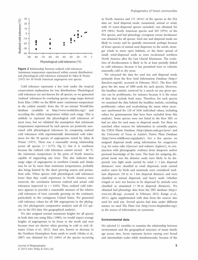
across all species (r = 0.773, Fig. 2), but it is nonlinear

because the realized cold tolerances cannot exceed �40 °C:the minimum temperature in the parts of North America

capable of supporting any trees. This also indicates that

range edges of angiosperms in northern Canada and Alaska

may be set by more than minimum temperatures, probably

also being limited by the short growing season and perma-

frost soils. When species with physiological cold tolerances

lower than they could experience in North America were

removed, the correlation between realized and actual cold

tolerances improved to r = 0.834. Thus, realized cold toler-

ance appears to provide a reasonable measure of the relative

cold tolerances of trees currently growing on the continent,

particularly in the contiguous United States. We generated

cold tolerance values for all 500 angiosperms in the phylog-

eny (for phylogenetic comparative analysis) and all 212 spe-

cies in the FIA data (for geographical analysis).

We also assigned normal maximum heights for all species

in both data sets using Elias (1980); we would expect average

heights of angiosperms to be lower to the north and west

because trees are shorter when growing in cold or arid cli-

mates (Lines et al., 2012). Seed size, known to decrease in

the Northern Hemisphere from south to north (Moles et al.,

2007) was obtained for 321 (64%) of the species occurring

in North America and 171 (81%) of the species in the FIA

data set. Seed dispersal mode (unassisted, animal or wind,

with 10 water-dispersed species excluded) was obtained for

479 (96%) North American species and 205 (97%) of the

FIA species, and leaf phenology (evergreen versus deciduous)

was obtained for all species. Seed size and dispersal mode are

likely to covary and be spatially structured, perhaps because

of fewer species of animal seed dispersers to the north, stron-

ger winds in more open habitats, or the faster spread of

small, wind-dispersed seeds as trees recolonized northern

North America after the Last Glacial Maximum. The evolu-

tion of deciduousness is likely to be at least partially linked

to cold tolerance, because it has permitted trees to colonize

seasonally cold or dry areas.

We extracted the data for seed size and dispersal mode

primarily from the Kew Seed Information Database (http://

data.kew.org/sid/, accessed in February 2012). The Kew SID

gives the dry mass of 1000 seeds for each species. However,

the headline statistic retrieved by a search on any given spe-

cies can be problematic, for instance because it is the mean

of data that include fresh mass. Therefore, for each species

we examined the data behind the headline statistic, excluding

problematic values and recalculating the mean when neces-

sary (performed for 120 of 1656 individual values, including

values for gymnosperms that have been excluded from this

analysis). Some species were not listed in the Kew SID, or

had no data for seed mass or dispersal mode. For these we

searched other sources for information in scientific papers,

the USDA Plants Database (http://plants.usda.gov/java/) and

the University of Texas at Austin’s Native Plant Database

(http://www.wildflower.org/plants/). For a few species we

assigned dispersal mode using information for congenerics

[e.g. for some oaks (Quercus) and walnuts (Juglans)], in con-

junction with photographic evidence from diaspores and/or

personal knowledge of the trees. The basis for assigning dis-

persal mode was the distance seeds were likely to be dis-

persed; very light seeds carried by wind (> 1 km dispersal

distances) were classified as wind dispersed, seeds carried

and/or eaten by birds and mammals were considered med-

ium dispersers (50 m to 1 km dispersal distance) and were

classified as animal dispersed, and heavy seeds (whether

winged or not) not known to be dispersed by animals were

classified as unassisted (< 50 m dispersal distances). We

obtained leaf phenology data from the TRY database (http://

www.try-db.org/, accessed in February 2012; Kattge et al.,

2011), again supplemented with data from the sources also

used for seed size. Several species had data under different

names; we used The Plant List (http://www.theplantlist.org/)

as the source of information on synonyms.

Environmental data

We selected 11 variables to examine the relationship between

environment and the geographical structure of mean family

age across sites. Seven represent factors varying over broad

and intermediate scales while simultaneously, because of the

Figure 2 Relationship between realized cold tolerances(minimum temperature experienced within current distribution)

and physiological cold tolerances estimated by Sakai & Weiser(1973) for 30 North American angiosperm tree species.


5


methods by which they were generated, having little or no

variation at local scales. We extracted two measures of tem-

perature and three of precipitation from the 30 arc-second

WorldClim database: BIO5 (maximum temperature of the

warmest month), BIO6 (minimum temperature of the coldest

month), BIO12 (annual precipitation), BIO9 (precipitation

in the driest quarter) and BIO18 (precipitation in the warm-

est quarter). The expectation is that minimum temperatures

should be the variable most strongly associated with mean

family age at the continental extent. We also calculated sum-

mer soil moisture, derived from the European Space Agency

global soil moisture data set (http://www.esa-soilmois-

ture-cci.org/, accessed in June 2012). Daily soil moistures

were averaged over 1 June to 31 August over five haphazardly

selected years with good coverage of North America (1983,

1995, 2000, 2005 and 2008). Although this variable contains

moderate patchiness at intermediate scales, the grain of com-

putation (c. 25 km) makes it unsuitable for examining local-

scale variation. Finally, we classified sites as being ice free or

glaciated during the Last Glacial Maximum, using the 18 ka

map of Dyke et al. (2003). The local communities at a mini-

mum of 30,437 of the sites in our analysis had to be assem-

bled through primary succession as the ice retreated.

We also generated four variables containing small-scale

variation to represent proxies for potential local processes.

We estimated the elevation of each site using the digital

elevation model gtopo30 (http://www1.gsi.go.jp/geowww/

globalmap-gsi/gtopo30/gtopo30.html), although this method

generates some error because the Forest Service shifts the

geographical coordinates of some sites slightly to protect the

privacy of private landowners. We extracted site slope and

aspect directly from the FIA database. Finally, we recorded

the categorical physiographic class code (PHYSCLCD), also

from the FIA, defined as ‘The general effect of land form,

topographical position, and soil on moisture available to

trees’ (http://fia.fs.fed.us/library/database-documentation/,

version 5.1 for Phase 2, p. 60). Although this highly local

variable might be expected to co-vary with the coarser,

remotely sensed ESA soil moisture, an ANOVA indicated no

relationship between them (model r2 = 0.003).

Analytical protocols

Phylogenetic comparative analyses (for testing prediction 4)

We used multiple approaches to evaluate evolutionary pat-

terns in the traits. First, we examined the phylogenetic sig-

nal of each tree trait using a phylogenetic signal

representation curve (PSR) approach (Diniz-Filho et al.,

2012), which is derived from phylogenetic eigenvector

regression (PVR; Diniz-Filho et al., 1998). In PVR, selected

eigenvectors extracted from a phylogenetic distance matrix

are used to model interspecific variation for a trait. In PSR,

sequential PVR models are fitted after successively increas-

ing the number of eigenvectors and plotting their R2 against

the accumulated eigenvalues extracted from the phylogenetic

distance matrix. Diniz-Filho et al. (2012) demonstrated that

under a Brownian motion model of evolution for quantita-

tive traits the relationship between the R2 values of the

PVRs and the cumulative eigenvalues is linear, and the pat-

tern of the deviations from linearity reflects alternative evo-

lutionary models. The PSR area, expressing deviations from

Brownian motion across the curve, is strongly correlated

with Blomberg’s K statistic, so nonlinear PSR curves reveal

whether traits are evolving at a slower or faster rate than

expected under Brownian motion in different parts of the

phylogeny (expressed by the location of deviations along the

eigenvalue axis). For example, in an Ornstein–Uhlenbeck

(OU) process, the PSR curve lies below the Brownian linear

expectation, and the PSR area is correlated with the strength

of the OU process (the a parameter, which can also be

expressed as phylogenetic half-life). Thus, PSR provides an

elegant exploratory method for understanding deviations

from Brownian motion in terms of acceleration or decelera-

tion of evolutionary rates at large or small phylogenetic dis-

tances. We used the pvr package in R (see http://cran.

r-project.org/web/packages/PVR/index.html) for calculating

the PSR curves for each quantitative species trait.

We also followed Kozak & Wiens (2010) and Wiens et al.

(2010) and tested for niche conservatism in each trait using

the general approach of Butler & King (2004). We calculated

the log-likelihood of phylogenetic generalized least squares

(pGLS) fitting of three models of evolution for each species

trait: a white noise (WN) model of random variation, in

which the similarity of species is independent of their phylo-

genetic relationships; a Brownian motion (BM) model of

gradual and continuous drift in species’ traits (sufficient to

demonstrate PNC according to one definition); and an Orn-

stein–Uhlenbeck (OU) model of constrained evolution (i.e.

stasis or stabilizing selection – see Hansen & Martins, 1996;

Hansen, 1997; Hansen et al., 2008), which satisfies the most

stringent definition of PNC (Losos, 2008). The first two mod-

els (WN and BM) do not explicitly incorporate constraints in

evolution, and the covariance among species will be indepen-

dent (WN) or linearly associated with phylogenetic related-

ness (BM). The OU model, in contrast, describes constrained

character evolution in which traits are ‘pulled’ towards an

optimum value (Kozak & Wiens, 2010), and even if the

restraining force (a) is strong enough to eliminate all phylo-

genetic signal, the variance of the trait will be much smaller

than expected under BM or WN models (although the latter

is difficult to assess in practice because there is no explicit

expectation of trait variance under alternative evolutionary

processes – see Revell et al., 2008). We used geiger in R

(Harmon et al., 2008) to calculate the log-likelihood of each

model and compared the fit of each model using a likelihood

test, converging to a chi-square distribution, to determine

whether each trait fits an OU model better than either a BM

or WN model. Weights of the Akaike information criterion

(AIC) derived from model likelihoods were also used as an

alternative approach to evaluate the best-fitting model (and

generated slightly different results).


6


Both PSR and fitting models using pGLS are designed

for quantitative traits, and expectations for discrete traits

may differ. So, for leaf phenology and seed dispersal mode

we used a simulation approach to obtain the distribution

of expected values of PSR area and the expected difference

between likelihoods of pGLS models. The observed values

of PSR area and likelihood differences were compared with

an empirical distribution of values obtained by simulating

250 Brownian motion processes on the phylogeny using

geiger. The simulated continuous traits were then trans-

formed into a discrete trait keeping the observed frequency

of the original trait (Fritz & Purvis, 2010) and then analy-

sed using the PSR curves and pGLS model fits for each

simulation.

Geographical analysis (for testing predictions 1–3)

Analysis of mean family age also followed several steps.

First, four random forest models were generated in Statis-

tica 8.0 to account statistically for MFA across sites, one

model including only traits, one including broad-scale envi-

ronmental predictors only, one including local-scale envi-

ronmental predictors only, and a combined model including

all predictors. One hundred regression trees were generated

in each run, and variable importance values and test risk

estimates (squared error rates) were recorded. Thus, the first

random forest model identified the most important traits

(as defined by the method and available traits), the second

identified the most important broad-scale environmental

predictors, the third identified the most important local-

scale environmental predictor, and the fourth ranked the

simultaneous contributions of all variables to MFA. Poten-

tial collinearity among predictors within each model can be

indicated by relative importance values from random forest

models, but it also was evaluated with general linear model-

ling. We first generated linear models that included the

most important predictor variable (environmental or trait)

identified by the random forest models and compared those

models against models in which all environmental, trait or

combined variables were included. Increases in the coeffi-

cient of determination represent the contribution of the

remaining variables not collinear with the most important

predictor.

Spatial evaluation (for testing predictions 2–3)

We evaluated the ability of the predictor variables to account

for the spatial structure of mean family age using spatial cor-

relograms generated in sam 4.0 (Rangel et al., 2010). Because

of computational limitations a correlogram for MFA was

generated based on 15,000 randomly selected sites. We then

generated a correlogram for the same subset of sites using

the residuals of the combined random forest model gener-

ated using all sites. The difference between the correlograms

quantifies the amounts of spatial pattern explained by the

model across scales and identifies any scales at which the

model is unable to fully explain the spatial pattern (Diniz-

Filho et al., 2003).

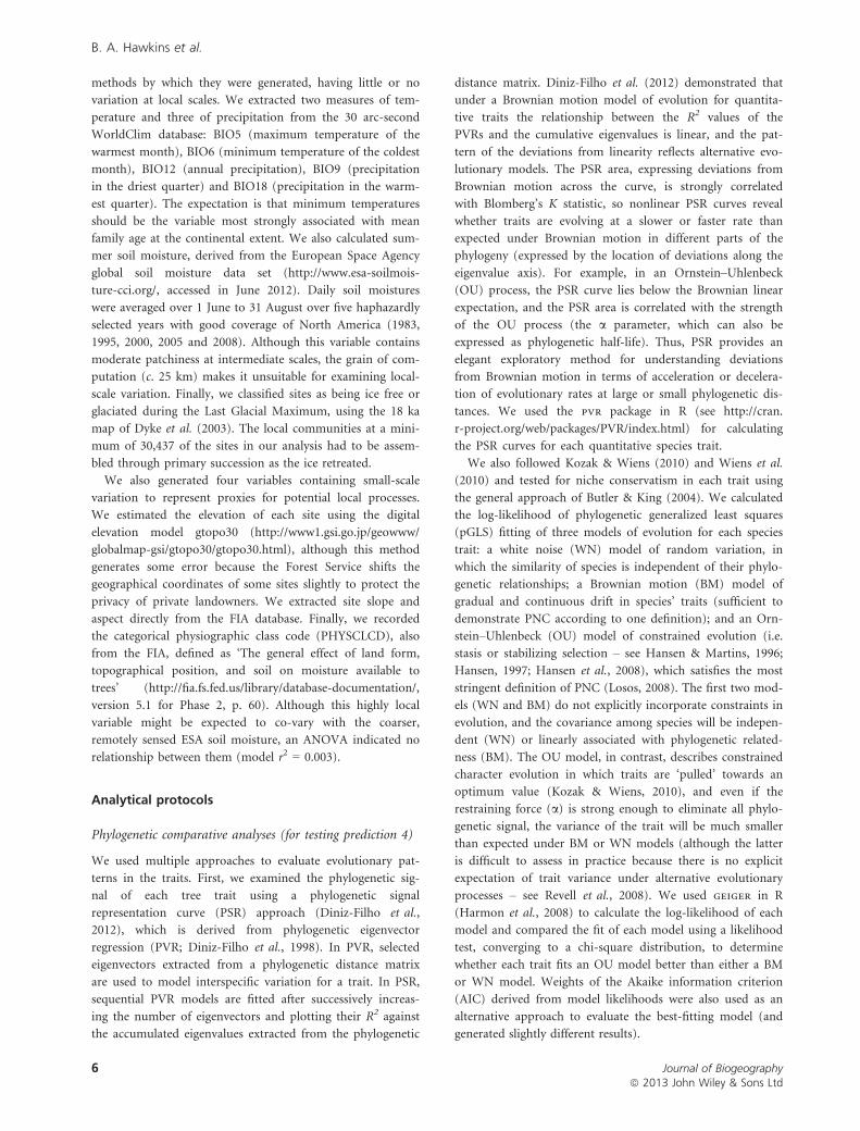
RESULTS

Mean family age shows geographical pattern across the

contiguous USA at almost all spatial scales whether using

molecular- or fossil-based ages (Fig. 3). Focusing on the

molecular-based results (Fig. 3a), at the larger scale there is a

striking ‘latitudinal’ gradient, with the angiosperm compo-

nent of forest communities dominated by trees from older

families in southern forests and from younger families to the

north. This is consistent among eastern, western-montane

and west-coast forests, although southern montane forests

tend to be younger than lowland forests at equivalent lati-

tudes. There are also regional longitudinal gradients, espe-

cially in the eastern forests, with lowland forests nearer the

east coast comprising older families than forests at the forest–

prairie interface. There is no evidence of a longitudinal gradi-

ent at the largest scale across the entire USA, because both

eastern and western forests show a pattern of older MFAs

near the coast in the south but younger ages to the north

(Fig. 3a). Mean fossil-based ages differ in several respects

(Fig. 3b), but many of the age estimates are imprecise given

Figure 3 Geographical pattern of mean family age for North

American angiosperm tree species across 91,340 plots based on(a) molecular dates from Davies et al. (2004), and (b) fossil

dates. Major rivers are shown in white. The insert in (a)exemplifies variation at local scales.


7


the current state of the fossil record. Most notable is that

average ages were substantially older in most places than

those using molecular-based family ages.

A few other patterns stand out at intermediate scales. For

example, Appalachian forests tend to be from younger fami-

lies than surrounding lowland sites, and forests along the

lower Mississippi River tend to comprise species from youn-

ger families than other southern forests to the east and west

for both age estimates (Fig. 3). Additional smaller-scale

patches also exist in various areas without obvious associated

geographical features. Finally, patchiness occurs down to the

smallest scale of the data, although there is also substantial

variation at very local scales: sites within a few kilometres of

each other can have very different mean family ages (Fig. 3a

insert). The structure of the data strongly implies that both

biogeographical and local factors influence the phylogenetic

structure of angiosperm tree communities across the central

section of the continent represented by the contiguous USA.

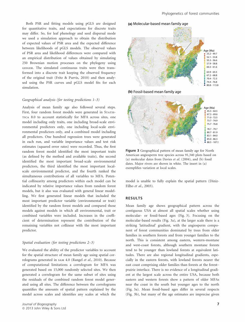
All five traits also contain broad- and local-scale pattern-

ing (Fig. 4), but correlations among them range from

non-existent (r = �0.029 for mean dispersal mode versus

mean height) to moderate (r = �0.598 for mean dispersal

mode versus mean cold tolerance). All patterns are broadly

consistent with what we might expect, such as more cold-tol-

erant species in the north (Fig. 4a), wind-dispersed and

small-seeded species composing northern forests (Fig. 4b,c),

evergreen-dominated forests to the south (recalling that gym-

nosperms have been excluded) (Fig. 4d), and shorter trees in

Figure 4 Geographical patterns of (a) mean realized cold tolerance, (b) geometric mean seed size, (c) mean ranked dispersal mode, (d)mean categorized leaf phenology and (e) mean normal maximum height across 91,340 plots for North American angiosperm tree

species. The black line in (a) delimits the extent of the ice sheets during the Last Glacial Maximum.


8


arid and semi-arid areas (Fig. 4e). Three traits, mean cold

tolerance, mean seed size and mean dispersal mode, also

show visibly one of the smaller scale patterns seen in MFA,

with sites close to the lower Mississippi River being more

similar to sites upriver than to adjacent southern areas (cf.

Figs 3 & 4a–c).

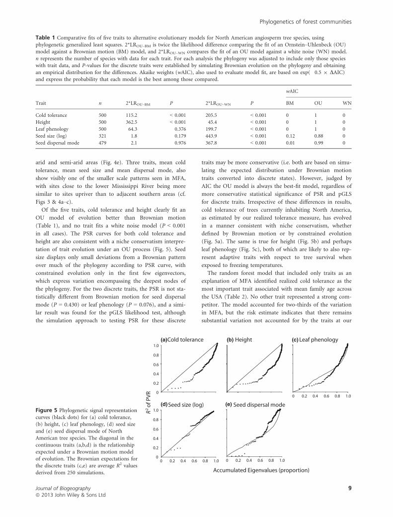
Of the five traits, cold tolerance and height clearly fit an

OU model of evolution better than Brownian motion

(Table 1), and no trait fits a white noise model (P < 0.001

in all cases). The PSR curves for both cold tolerance and

height are also consistent with a niche conservatism interpre-

tation of trait evolution under an OU process (Fig. 5). Seed

size displays only small deviations from a Brownian pattern

over much of the phylogeny according to PSR curve, with

constrained evolution only in the first few eigenvectors,

which express variation encompassing the deepest nodes of

the phylogeny. For the two discrete traits, the PSR is not sta-

tistically different from Brownian motion for seed dispersal

mode (P = 0.430) or leaf phenology (P = 0.076), and a simi-

lar result was found for the pGLS likelihood test, although

the simulation approach to testing PSR for these discrete

traits may be more conservative (i.e. both are based on simu-

lating the expected distribution under Brownian motion

traits converted into discrete states). However, judged by

AIC the OU model is always the best-fit model, regardless of

more conservative statistical significance of PSR and pGLS

for discrete traits. Irrespective of these differences in results,

cold tolerance of trees currently inhabiting North America,

as estimated by our realized tolerance measure, has evolved

in a manner consistent with niche conservatism, whether

defined by Brownian motion or by constrained evolution

(Fig. 5a). The same is true for height (Fig. 5b) and perhaps

leaf phenology (Fig. 5c), both of which are likely to also rep-

resent adaptive traits with respect to tree survival when

exposed to freezing temperatures.

The random forest model that included only traits as an

explanation of MFA identified realized cold tolerance as the

most important trait associated with mean family age across

the USA (Table 2). No other trait represented a strong com-

petitor. The model accounted for two-thirds of the variation

in MFA, but the risk estimate indicates that there remains

substantial variation not accounted for by the traits at our

Table 1 Comparative fits of five traits to alternative evolutionary models for North American angiosperm tree species, using

phylogenetic generalized least squares. 2*LROU–BM is twice the likelihood difference comparing the fit of an Ornstein–Uhlenbeck (OU)model against a Brownian motion (BM) model, and 2*LROU–WN compares the fit of an OU model against a white noise (WN) model.

n represents the number of species with data for each trait. For each analysis the phylogeny was adjusted to include only those specieswith trait data, and P-values for the discrete traits were established by simulating Brownian evolution on the phylogeny and obtaining

an empirical distribution for the differences. Akaike weights (wAIC), also used to evaluate model fit, are based on exp(�0.5 9 DAIC)and express the probability that each model is the best among those compared.

Trait n 2*LROU–BM P 2*LROU–WN P

wAIC

BM OU WN

Cold tolerance 500 115.2 < 0.001 205.5 < 0.001 0 1 0

Height 500 362.5 < 0.001 45.4 < 0.001 0 1 0

Leaf phenology 500 64.3 0.376 199.7 < 0.001 0 1 0

Seed size (log) 321 1.8 0.179 443.9 < 0.001 0.12 0.88 0

Seed dispersal mode 479 2.1 0.976 367.8 < 0.001 0.01 0.99 0

Figure 5 Phylogenetic signal representation

curves (black dots) for (a) cold tolerance,(b) height, (c) leaf phenology, (d) seed size

and (e) seed dispersal mode of NorthAmerican tree species. The diagonal in the

continuous traits (a,b,d) is the relationshipexpected under a Brownian motion model

of evolution. The Brownian expectations forthe discrete traits (c,e) are average R2 values

derived from 250 simulations.


9


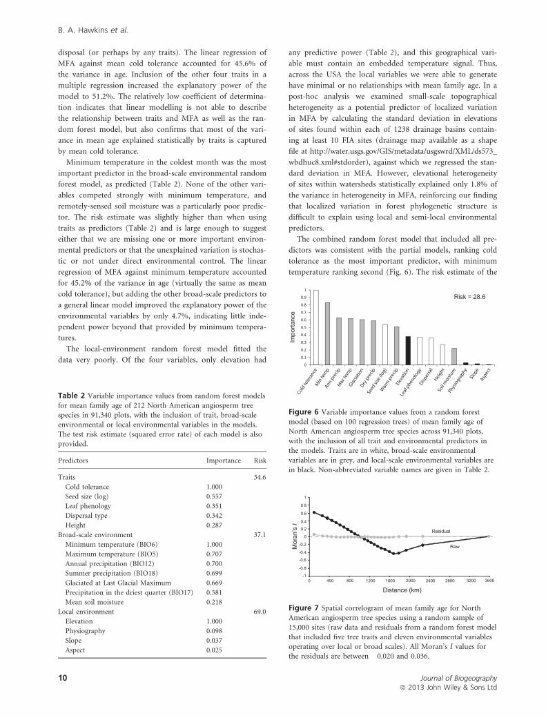
disposal (or perhaps by any traits). The linear regression of

MFA against mean cold tolerance accounted for 45.6% of

the variance in age. Inclusion of the other four traits in a

multiple regression increased the explanatory power of the

model to 51.2%. The relatively low coefficient of determina-

tion indicates that linear modelling is not able to describe

the relationship between traits and MFA as well as the ran-

dom forest model, but also confirms that most of the vari-

ance in mean age explained statistically by traits is captured

by mean cold tolerance.

Minimum temperature in the coldest month was the most

important predictor in the broad-scale environmental random

forest model, as predicted (Table 2). None of the other vari-

ables competed strongly with minimum temperature, and

remotely-sensed soil moisture was a particularly poor predic-

tor. The risk estimate was slightly higher than when using

traits as predictors (Table 2) and is large enough to suggest

either that we are missing one or more important environ-

mental predictors or that the unexplained variation is stochas-

tic or not under direct environmental control. The linear

regression of MFA against minimum temperature accounted

for 45.2% of the variance in age (virtually the same as mean

cold tolerance), but adding the other broad-scale predictors to

a general linear model improved the explanatory power of the

environmental variables by only 4.7%, indicating little inde-

pendent power beyond that provided by minimum tempera-

tures.

The local-environment random forest model fitted the

data very poorly. Of the four variables, only elevation had

any predictive power (Table 2), and this geographical vari-

able must contain an embedded temperature signal. Thus,

across the USA the local variables we were able to generate

have minimal or no relationships with mean family age. In a

post-hoc analysis we examined small-scale topographical

heterogeneity as a potential predictor of localized variation

in MFA by calculating the standard deviation in elevations

of sites found within each of 1238 drainage basins contain-

ing at least 10 FIA sites (drainage map available as a shape

file at http://water.usgs.gov/GIS/metadata/usgswrd/XML/ds573_

wbdhuc8.xml#stdorder), against which we regressed the stan-

dard deviation in MFA. However, elevational heterogeneity

of sites within watersheds statistically explained only 1.8% of

the variance in heterogeneity in MFA, reinforcing our finding

that localized variation in forest phylogenetic structure is

difficult to explain using local and semi-local environmental

predictors.

The combined random forest model that included all pre-

dictors was consistent with the partial models, ranking cold

tolerance as the most important predictor, with minimum

temperature ranking second (Fig. 6). The risk estimate of the

Table 2 Variable importance values from random forest models

for mean family age of 212 North American angiosperm treespecies in 91,340 plots, with the inclusion of trait, broad-scale

environmental or local environmental variables in the models.The test risk estimate (squared error rate) of each model is also

provided.

Predictors Importance Risk

Traits 34.6

Cold tolerance 1.000

Seed size (log) 0.557

Leaf phenology 0.351

Dispersal type 0.342

Height 0.287

Broad-scale environment 37.1

Minimum temperature (BIO6) 1.000

Maximum temperature (BIO5) 0.707

Annual precipitation (BIO12) 0.700

Summer precipitation (BIO18) 0.699

Glaciated at Last Glacial Maximum 0.669

Precipitation in the driest quarter (BIO17) 0.581

Mean soil moisture 0.218

Local environment 69.0

Elevation 1.000

Physiography 0.098

Slope 0.037

Aspect 0.025

Figure 6 Variable importance values from a random forest

model (based on 100 regression trees) of mean family age ofNorth American angiosperm tree species across 91,340 plots,

with the inclusion of all trait and environmental predictors inthe models. Traits are in white, broad-scale environmental

variables are in grey, and local-scale environmental variables arein black. Non-abbreviated variable names are given in Table 2.

0

0.2

0.4

0.6

0.8

1

0 400 800 1200 1600 2000 2400 2800 36003200

-0.8

-0.6

-0.4

-1

-0.2

Distance (km)

Mor

an’s

I

Raw

Residual

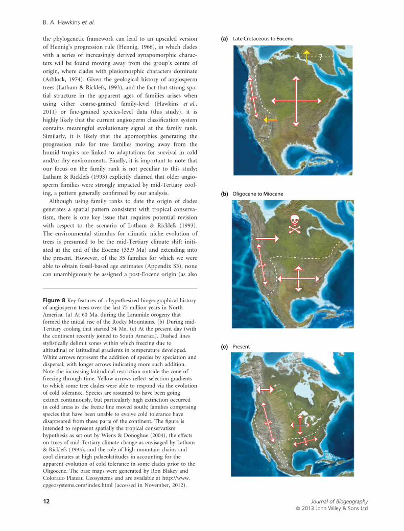
Figure 7 Spatial correlogram of mean family age for NorthAmerican angiosperm tree species using a random sample of

15,000 sites (raw data and residuals from a random forest modelthat included five tree traits and eleven environmental variables

operating over local or broad scales). All Moran’s I values forthe residuals are between �0.020 and 0.036.


10


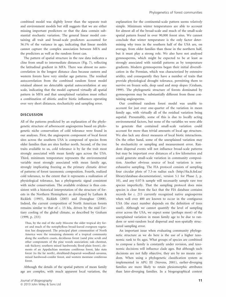
combined model was slightly lower than the separate trait

and environment models but still suggests that we are either

missing important predictors or that the data contain sub-

stantial stochastic variation. The general linear model con-

taining all trait and broad-scale predictors accounted for

56.1% of the variance in age, indicating that linear models

cannot capture the complex association between MFA and

the predictors as well as the random forest can.

The pattern of spatial structure in the raw data indicates a

cline from small to intermediate distances (Fig. 7), reflecting

the latitudinal gradient in MFA. There was almost no auto-

correlation in the longest distance class because eastern and

western forests have very similar age patterns. The residual

autocorrelation from the combined random forest model

retained almost no detectable spatial autocorrelation at any

scale, indicating that the model captured virtually all spatial

pattern in MFA and that unexplained variation must reflect

a combination of abiotic and/or biotic influences operating

over very short distances, stochasticity and sampling error.

DISCUSSION

All of the patterns predicted by an explanation of the phylo-

genetic structure of arborescent angiosperms based on phylo-

genetic niche conservatism of cold tolerance were found in

our analyses. First, the angiosperm component of local forest

sites across the southern USA is composed of species from

older families than are sites further north. Second, of the tree

traits available to us, cold tolerance is by far the trait most

strongly associated with mean family ages across the USA.

Third, minimum temperature represents the environmental

variable most strongly associated with mean family age,

strongly implicating freezing as the primary climatic driver

of patterns of forest taxonomic composition. Fourth, realized

cold tolerance, to the extent that it represents a realization of

physiological tolerance, has a phylogenetic signal consistent

with niche conservatism. The available evidence is thus con-

sistent with a historical interpretation of the structure of for-

ests in the Northern Hemisphere as developed by Latham &

Ricklefs (1993), Ricklefs (2005) and Donoghue (2008).

Indeed, the current composition of North American forests

remains similar to that of c. 15 Ma, driven by the mid-Ter-

tiary cooling of the global climate, as described by Graham

(1999, p. 233):

Thus, by the end of the early Miocene the older tropical dry for-

est and much of the notophyllous broad-leaved evergreen vegeta-

tion has disappeared. The principal plant communities of North

America were the remaining elements of a tropical community

along the southern coasts, deciduous forest (sand pine scrub and

other components of the pine woods association; oak–chestnut,oak–hickory; southern mixed hardwoods; flood-plain forest), ele-

ments of an Appalachian montane coniferous forest, lake state

forest (to the far north), shrubland/chaparral–woodland–savanna,mixed hardwood–conifer forest, and western montane coniferous

forest.

Although the details of the spatial pattern of mean family

age are complex, with much apparent local variation, the

explanation for the continental-scale pattern seems relatively

simple. Minimum winter temperatures are able to account

for almost all of the broad-scale and much of the small-scale

spatial pattern found in over 90,000 forest sites. We cannot

conclude that winter temperature is the only factor deter-

mining why trees in the southern half of the USA are, on

average, from older families than those in the northern half,

but it must play a strong role. We also have not analysed

gymnosperms, which might be expected to be at least as

strongly associated with rainfall patterns as by temperature

gradients. Modern gymnosperms began their initial diversifi-

cation in the Permian, which was characterized by extensive

aridity, and consequently they have a number of traits that

provide physiological drought tolerance, permitting them to

survive on frozen soils, deep sand and steep slopes (Graham,

1999). The phylogenetic structure of forests dominated by

gymnosperms may be substantially different from those con-

taining angiosperms.

Our combined random forest model was unable to

account for just over one-quarter of the variation in mean

family age, with virtually all of the residual variation being

aspatial. Presumably, some of this is due to locally acting

environmental factors, but none of the variables we were able

to generate that contained small-scale variation could

account for more than trivial amounts of local age structure.

We also lack any direct measures of local biotic interactions.

On the other hand, some of the unexplained variation may

be stochasticity or sampling and measurement error. Ran-

dom dispersal events will not influence broad-scale patterns

but may be important over distances of a few kilometres and

could generate small-scale variation in community composi-

tion. Another obvious source of local variation is non-

exhaustive sampling. The FIA protocol consists of sampling

four circular plots of 7.3-m radius each (http://fia.fs.fed.us/

library/database-documentation/, version 5.1 for Phase 2, p.

10), and any 0.07-h sample will necessarily sample rare tree

species imperfectly. That the sampling protocol does miss

species is clear from the fact that the FIA database contains

records for c. 215 currently recognized native angiosperms

when well over 400 are known to occur in the contiguous

USA (the exact number depends on the definition of trees

used). Although we cannot quantify the level of sampling

error across the USA, we expect some (perhaps most) of the

unexplained variation in mean family age to be due to ran-

dom or semi-random local dispersal and non-spatially struc-

tured sampling error.

An important issue when evaluating community phyloge-

netic structure as we do here is the use of a higher taxo-

nomic rank to fix ages. What groups of species are combined

to compose a family is constantly under revision, and taxo-

nomic decisions will influence clade ages. But although such

decisions are not fully objective, they are by no means ran-

dom. When using a phylogenetic classification system as

implemented in APG III (Stevens, 2001), earlier-diverging

families are more likely to retain plesiomorphic attributes

than later-diverging families. In a biogeographical context


11


the phylogenetic framework can lead to an upscaled version

of Hennig’s progression rule (Hennig, 1966), in which clades

with a series of increasingly derived synapomorphic charac-

ters will be found moving away from the group’s centre of

origin, where clades with plesiomorphic characters dominate

(Ashlock, 1974). Given the geological history of angiosperm

trees (Latham & Ricklefs, 1993), and the fact that strong spa-

tial structure in the apparent ages of families arises when

using either coarse-grained family-level (Hawkins et al.,

2011) or fine-grained species-level data (this study), it is

highly likely that the current angiosperm classification system

contains meaningful evolutionary signal at the family rank.

Similarly, it is likely that the apomorphies generating the

progression rule for tree families moving away from the

humid tropics are linked to adaptations for survival in cold

and/or dry environments. Finally, it is important to note that

our focus on the family rank is not peculiar to this study;

Latham & Ricklefs (1993) explicitly claimed that older angio-

sperm families were strongly impacted by mid-Tertiary cool-

ing, a pattern generally confirmed by our analysis.

Although using family ranks to date the origin of clades

generates a spatial pattern consistent with tropical conserva-

tism, there is one key issue that requires potential revision

with respect to the scenario of Latham & Ricklefs (1993).

The environmental stimulus for climatic niche evolution of

trees is presumed to be the mid-Tertiary climate shift initi-

ated at the end of the Eocene (33.9 Ma) and extending into

the present. However, of the 35 families for which we were

able to obtain fossil-based age estimates (Appendix S3), none

can unambiguously be assigned a post-Eocene origin (as also

Figure 8 Key features of a hypothesized biogeographical historyof angiosperm trees over the last 75 million years in North

America. (a) At 60 Ma, during the Laramide orogeny thatformed the initial rise of the Rocky Mountains. (b) During mid-

Tertiary cooling that started 34 Ma. (c) At the present day (withthe continent recently joined to South America). Dashed lines

stylistically delimit zones within which freezing due toaltitudinal or latitudinal gradients in temperature developed.

White arrows represent the addition of species by speciation anddispersal, with longer arrows indicating more such addition.

Note the increasing latitudinal restriction outside the zone offreezing through time. Yellow arrows reflect selection gradients

to which some tree clades were able to respond via the evolutionof cold tolerance. Species are assumed to have been going

extinct continuously, but particularly high extinction occurredin cold areas as the freeze line moved south; families comprising

species that have been unable to evolve cold tolerance havedisappeared from these parts of the continent. The figure is

intended to represent spatially the tropical conservatismhypothesis as set out by Wiens & Donoghue (2004), the effects

on trees of mid-Tertiary climate change as envisaged by Latham

& Ricklefs (1993), and the role of high mountain chains andcool climates at high palaeolatitudes in accounting for the

apparent evolution of cold tolerance in some clades prior to theOligocene. The base maps were generated by Ron Blakey and

Colorado Plateau Geosystems and are available at http://www.cpgeosystems.com/index.html (accessed in November, 2012).


12


noted and discussed by Latham & Ricklefs, 1993). Thus,

there is apparently a substantial temporal mismatch between

the timing of the selective event and the ages of the clades

that presumably responded. We are left with an important

question: if essentially all tree families originated before the

Oligocene climate shift, why did taxa in relatively young

groups evolve cold tolerance, permitting them to occupy the

newly created cold regions, whereas taxa in relatively older

families did not, retreating towards the tropics? We have no

direct evidence that might account for this, but the initial

rise of the Rocky Mountains spanning the Late Cretaceous to

the Palaeocene (80–55 Ma; English & Johnston, 2004) may

have provided the selective force for the evolution of cold

tolerance, perhaps coupled with the development of relatively

cold climates at high palaeolatitudes in the Late Cretaceous

(Wing & Sues, 1992). That is, the selection for cold tolerance

could have begun when angiosperm families were originating

well before the Eocene Thermal Optimum, pre-adapting

many clades for expansion into the newly created lowland

cold climatic regimes generated in the Oligocene (see Fig. 8

for how this hypothesis can account for current patterns in

the face of strong niche conservatism). This aspect of the

tropical conservatism hypothesis vis-�a-vis trees requires addi-

tional work, but it does not alter the observation that forest

communities to the north are dominated by species from

younger families than are those to the south, a pattern that

begs for an explanation.

Patterns of trait evolution further point towards phyloge-

netic niche conservatism as influencing North American tree

distributions. Under the interpretations of Losos (2008) and

Wiens et al. (2010), finding that a trait fits an OU model is

consistent with PNC. The pattern of nonlinear evolution

slower than BM is also expected under the phylogenetic iner-

tia and niche filling models of Cooper et al. (2010). The rela-

tionship between PNC and phylogenetic signal is not direct

and is not easy to establish in practice, because strong PNC

(for instance, very strong stabilizing selection modelled as an

OU process with a high a) can eliminate phylogenetic pat-

terns of covariance among species, mimicking a white noise

model. There is also no consensus as to whether phylogenetic

signal per se (e.g. Brownian motion evolution) is sufficient

to be considered phylogenetic niche conservatism, or more

constrained patterns of evolution are required. Irrespective, it

remains that for the key trait in our analysis, cold tolerance,

a substantially better fit to an OU model and the nonlinear

PSR curve are evidence for PNC, however defined, because

phylogenetic signal exists and the covariance structure among

species has been constrained and divergence has been sub-

stantially slowed when compared with Brownian expecta-

tions. Among the continuous traits seed size comes closest to

fitting a Brownian motion model, but it is not strongly asso-

ciated with mean family age. The discrete traits are also per-

haps not conserved as the process is defined by Losos (2008)

(although both contain phylogenetic signal), but they are not

strong predictors of mean family age.

All average trait values of local tree communities are spa-

tially structured, but average cold tolerance is by far most

closely associated with the family-rank ages of the trees. That

tree traits are associated with climate has been established in

the eastern United States (Swenson & Weiser, 2010), and

seed size in particular decreases latitudinally and is known to

contain phylogenetic signal (Moles et al., 2007). However,

Moles et al. (2007) attributed the gradient primarily to geo-

graphical shifts in plant growth form, which cannot account

for the gradient in our data, because all species are trees.

Swenson et al. (2012) also found geographical patterns in six

traits of woody plants across the Western Hemisphere,

including maximum height and seed mass, but our data are

restricted to angiosperm trees and perhaps for this reason

generate different patterns than they found. Although even a

cursory examination of the broad-scale patterns of traits

invites speculation about adaptive responses of trees to cli-

mate, we are focused on understanding why southern forests

contain species from older families than northern forests,

and only average cold tolerance seems to offer a reasonable

explanation.

One smaller-scale pattern across multiple traits merits

special mention. Forests from eastern Texas to northern

Florida are generally composed of angiosperms that are

from older families (Fig. 3), cold intolerant (Fig. 4a), seed-

dispersed by animals or unassisted (Fig. 4c), and a mix of

deciduous and evergreen species (Fig. 4d). In contrast, for-

ests growing along the lower Mississippi River have aver-

ages much more similar to forests in the central and upper

mid-western states. This suggests some interesting scenarios.

First, as the Laurentide Ice Sheet retreated with the arrival

of the current interglacial period, angiosperms colonizing

newly exposed sites were primarily cold tolerant, wind dis-

persed and deciduous. After the drainage of glacial meltwa-

ter was re-established to the Gulf of Mexico via the

Mississippi River Basin, after having been diverted to the

North Atlantic through the Great Lakes and the Gulf of St

Lawrence during the Younger Dryas (Broecker et al., 1989),

significant down-river dispersal from the establishing north-

ern forests probably occurred (see also Graham, 1999, for

discussion of this phenomenon), reversing the generalized

directional pattern of post-Pleistocene recolonization of

northern North America by trees (Davis et al., 1986; Ordo-

nez & Williams, 2013). An alternative, that the lower Mis-

sissippi retains species compositions that were forced into a

refugium as the most recent Ice Age developed, is possible

but less likely given the probable distribution of forest refu-

gia in eastern North America (Loehle, 2007). A third possi-

bility is that the regular historical disturbance from

Mississippi flooding favoured generalist species that are

more similar to those found much further north (Jocque

et al., 2010). Whichever scenario best describes the patterns

along the lower Mississippi River, it illustrates that although

cold tolerance is probably a primary driver of local com-

munity structure of North American forests, it is not the


13


only one, and explanations for local patterns depend on the

region being evaluated.

A final note related to the Laurentide Ice Sheet is that

although it necessitated the regeneration of forests de novo as

it retreated northwards, it seems to have left little imprint as

quantified in the environmental model of mean family age.

We cannot conclude that its influence was nil, but covaria-

tion with the current climatic gradient makes it difficult to

identify clear impacts at the continental extent.

Our combined random forest model accounted for

almost three-quarters of the variance in mean family age,

with almost no residual spatial structure in the data at any

scale. This indicates that no additional spatially structured

predictors are needed to account for the spatial pattern.

But it also leaves open the question of the extent to which

the unexplained phylogenetic age structure of angiosperm

forest communities represents deterministic, local abiotic/

biotic processes or stochasticity arising from random (or

neutral) local assembly and/or sampling error. The level of

variance accounted for by the model suggests that local

processes play a lesser role in community assembly than

biogeographical processes, but without direct evidence this

remains a supposition. Teasing apart the contributions of

local versus regional processes to local community structure

remains a core goal of community ecology. Here we have

focused primarily on regional factors, which is one step

towards understanding community phylogenetic structure at

all scales.

REFERENCES

Angiosperm Phylogeny Group (2009) An update of the

Angiosperm Phylogeny Group classification for the orders

and families of flowering plants: APG III. Botanical Journal

of the Linnean Society, 161, 105–121.

Ashlock, P.D. (1974) The uses of cladistics. Annual Review of

Ecology and Systematics, 5, 81–99.

Bell, C.D., Soltis, D.E. & Soltis, P.S. (2010) The age and

diversification of the angiosperms rerevisited. American

Journal of Botany, 97, 1296–1303.

Broecker, W.S., Kennett, J.P., Flower, B.P., Teller, J.T.,

Trumbore, S., Bonani, G. & Wolf, W. (1989) Routing of

meltwater from the Laurentide Ice Sheet during the

Younger Dryas cold episode. Nature, 341, 318–321.

Butler, M.A. & King, A.A. (2004) Phylogenetic comparative

analysis: a modeling approach for adaptive evolution. The

American Naturalist, 164, 683–695.

Cooper, N., Jetz, W. & Freckleton, R.P. (2010) Phylogenetic

comparative approaches for studying niche conservatism.

Journal of Evolutionary Biology, 23, 2529–2539.

Davies, T.J., Barraclough, T.G., Chase, M.W., Soltis, P.S.,

Soltis, D.E. & Savolainen, V. (2004) Darwin’s abominable

mystery: insights from a supertree of the angiosperms.

Proceedings of the National Academy of Sciences USA, 101,

1904–1909.

Davis, M.B., Woods, K.D., Webb, S.L. & Futyma, R.P.

(1986) Dispersal versus climate: expansion of Fagus and

Tsuga into the upper Great Lakes region. Vegetatio, 67,

93–103.

Diniz-Filho, J.A.F., Ramos de Sant’Ana, C.E. & Bini, L.M.

(1998) An eigenvector method for estimating phylogenetic

intertia. Evolution, 52, 1247–1262.

Diniz-Filho, J.A.F., Bini, L.M. & Hawkins, B.A. (2003) Spatial

autocorrelation and red herrings in geographical ecology.

Global Ecology and Biogeography, 12, 53–64.

Diniz-Filho, J.A.F., Rangel, T.F., Santos, T. & Bini, L.M.

(2012) Exploring patterns of interspecific variation in

quantitative traits using sequential phylogenetic eigenvec-

tor regressions. Evolution, 66, 1079–1090.

Donoghue, M.J. (2008) A phylogenetic perspective on the

distribution of plant diversity. Proceedings of the National

Academy of Sciences USA, 105(Suppl. 1), 11549–11555.

Drescher, M. & Thomas, S.C. (2013) Snow cover manipula-

tions alter survival of early life stages of cold-temperate

tree species. Oikos, 122, 541–554.

Dyke, A. S., Moore, A. & Robertson, L. (2003) Deglaciation

of North America. Geological Survey of Canada Open File

1574, Ottawa.

Elias, T. S. (1980) The complete trees of North America. Field

guide and natural history. Times Mirror Magazines, New

York.

English, J.M. & Johnston, S.T. (2004) The Laramide orogeny:

what were the driving forces? International Geology Review,

46, 833–838.

Fritz, S.A. & Purvis, A. (2010) Selectivity in mammalian

extinction risk and threat types: a new measure of phylo-

genetic signal strength in binary traits. Conservation Biol-

ogy, 24, 1042–1051.

Graham, A. (1999) Late Cretaceous and Cenozoic history of

North American vegetation. Oxford University Press, New

York.

Hansen, T.F. (1997) Stabilizing selection and the comparative

analysis of adaptation. Evolution, 51, 1341–1351.

Hansen, T.F. & Martins, E.P. (1996) Translating between

microevolutionary process and macroevolutionary pat-

terns: the correlation structure of interspecific data. Evolu-

tion, 50, 1404–1417.

Hansen, T.F., Piennar, J. & Orzack, S.H. (2008) A compara-

tive method for studying adaptation to a randomly evolv-

ing environment. Evolution, 62, 1965–1977.

Harmon, L.J., Weir, J.T., Brock, C.D., Glor, R.E. & Chal-

lenger, W. (2008) GEIGER: investigating evolutionary

radiations. Bioinformatics, 24, 129–131.

Hawkins, B.A., Rodr�ıguez, M.�A. & Weller, S.G. (2011) Global

angiosperm family richness revisited: linking ecology and

evolution to climate. Journal of Biogeography, 38, 1253–

1266.

Hennig, W. (1966) Phylogenetic systematics (translated by D.

D. Davis and R. Zangeri). University of Illinois Press,

Urbana, IL.


14


Hsu, J. (1983) Late Cretaceous and Cenozoic vegetation in

China, emphasizing their connection with North America.

Annals of the Missouri Botanical Garden, 70, 490–508.

Jocque, M., Field, R., Brendonck, L. & de Meester, L. (2010)

Climatic control of dispersal–ecological specialization

trade-offs: a metacommunity process at the heart of the

latitudinal diversity gradient? Global Ecology and Biogeogra-

phy, 19, 244–252.

Kattge, J., D�ıaz, S., Lavorel, S. et al. (2011) TRY – a global

database of plant traits. Global Change Biology, 17, 2905–

2935.

Koehler, K., Center, A. & Cavender-Bares, J. (2012) Evidence

for a freezing tolerance–growth rate trade-off in the live

oaks (Quercus series Virentes) across the tropical–temper-

ate divide. New Phytologist, 193, 730–744.

Kozak, K.H. & Wiens, J.J. (2010) Niche conservatism drives

elevational diversity patterns in Appalachian salamanders.

The American Naturalist, 176, 40–54.

Kunstler, G., Lavergne, S.L., Courbaud, B., Thuiller, W., Vie-

illedent, G., Zimmermann, N.E., Kattge, J. & Coomes,

D.A. (2012) Competitive interactions between forest trees

are driven by species’ trait hierarchy, not phylogenetic or

functional similarity: implications for forest community

assembly. Ecology Letters, 15, 831–840.

Latham, E. L. & Ricklefs, R. E. (1993) Continental compari-

sons of temperate-zone tree species diversity. Species diver-

sity in ecological communities: historical and geographical

perspectives (ed. by R. E. Ricklefs and D. Schluter), pp.

294–314. University of Chicago Press, Chicago, IL.

Lessard, J.-P., Borregaard, M.K., Fordyce, J.A., Rahbek, C.,

Weiser, M.D., Dunn, R.R. & Sanders, N.J. (2012) Strong

influence of regional species pools on continent-wide

structuring of local communities. Proceedings of the Royal

Society B: Biological Sciences, 279, 266–274.

Lines, E.R., Zavala, M.A., Purves, D.W. & Coomes, D.A.

(2012) Predictable changes in aboveground allometry

of trees along gradients of temperature, aridity and

competition. Global Ecology and Biogeography, 21, 1017–

1028.

Loehle, C. (2007) Predicting Pleistocene climate from vegeta-

tion in North America. Climates of the Past, 3, 109–118.

Losos, J.B. (2008) Phylogenetic niche conservatism, phyloge-

netic signal and the relationship between phylogenetic

relatedness and ecological similarly among species. Ecology

Letters, 11, 995–1007.

Moles, A.T., Ackerly, D.D., Tweddle, J.C., Dickie, J.B., Smith,

R., Leishman, M.R., Mayfield, M.M., Pitman, A., Wood,

J.T. & Westoby, M. (2007) Global patterns in seed size.

Global Ecology and Biogeography, 16, 109–116.

Ordonez, A. & Williams, J.W. (2013) Climatic and biotic

velocities for woody taxa distributions over the last

16,000 years in eastern North America. Ecology Letters, 16,

773–781.

Rangel, T.F., Diniz-Filho, J.A.F. & Bini, L.M. (2010) SAM: a

comprehensive application for spatial analysis in macroe-

cology. Ecography, 33, 46–60.

Revell, L.J., Harmon, L.J. & Collar, D.C. (2008) Phylogenetic

signal, evolutionary process, and rate. Systematic Biology,

57, 591–601.

Ricklefs, R.E. (2005) Historical and ecological dimensions of

global patterns in plant diversity. Biologiske Skrifter, 55,

583–603.

Sakai, A. & Weiser, C.J. (1973) Freezing resistance of trees in

North America with reference to tree regions. Ecology, 54,

118–126.

Smith, S.A. & Beaulieu, J.M. (2009) Life history influences

rates of climatic niche evolution in flowering plants. Pro-

ceedings of the National Academy of Sciences USA, 276,

4345–4352.

Smith, S.A., Beaulieu, J.M., Stamatakis, A. & Donoghue, M.J.

(2011) Understanding angiosperm diversification using

small and large phylogenetic trees. American Journal of

Botany, 98, 404–411.

Stevens, P. F. (2001) Angiosperm phylogeny website. Version

12, July 2012. Available at: http://www.mobot.org/

MOBOT/research/APweb/.

Swenson, N.G. & Weiser, M.D. (2010) Plant geography upon

the basis of functional traits: an example from eastern

North American trees. Ecology, 91, 2234–2241.

Swenson, N.G., Enquist, B.J., Pither, J. et al. (2012) The bio-

geography and filtering of woody plant functional diversity

in North and South America. Global Ecology and Biogeog-

raphy, 21, 798–808.

Webb, C.O., Ackerly, D.D. & Kembel, S.W. (2008) Phylo-

com: software for the analysis of phylogenetic community

structure and trait evolution. Bioinformatics, 24, 2098–

2100.

White, E.P. & Hurlbert, A.H. (2010) The combined influ-

ence of the local environment and regional enrichment

on bird species richness. The American Naturalist, 175,

E35–E43.

Wiens, J.J. & Donoghue, M.J. (2004) Historical biogeogra-

phy, ecology and species richness. Trends in Ecology and

Evolution, 19, 639–644.

Wiens, J.J., Ackerly, D.D., Allen, A.P., Anacker, B.L., Buckley,

L.B., Cornell, H.V., Damschen, E.I., Davies, T.J., Grytnes,

J.-A., Harrison, S.P., Hawkins, B.A., Holt, R.D., McCain,

C.M. & Stephens, P.R. (2010) Niche conservatism as an

emerging principle in ecology and conservation biology.

Ecology Letters, 13, 1310–1324.

Wing, S. K. & Sues, H.-D. (1992) Mesozoic and early Ceno-

zoic terrestrial ecosystems. Terrestrial ecosystems through

time (ed. by A. K. Behrensmeyer, J. D. Damuth, W. A.

DiMichele, R. Potts, H.-D. Sues and S. L. Wing), pp. 327–

416. University of Chicago Press, Chicago, IL.


15


SUPPORTING INFORMATION

Additional Supporting Information may be found in the

online version of this article:

Appendix S1 Sources used to construct the generic and

species nodes of the North American tree phylogeny and the

complete phylogeny in Newick format.

Appendix S2 High resolution graphical version of the phy-

logeny of North American trees.

Appendix S3 List of tree species, including family ages and

trait values.

BIOSKETCH

Bradford A. Hawkins is interested in ecological and phylo-

genetic patterns across a range of spatial scales, with a focus

on linking local and biogeographical processes.

Author contributions: B.A.H. conceived the idea, created the

phylogeny, conducted the geographical analyses and wrote

the first draft of the manuscript. M.R. generated the commu-

nity data and some trait data and conducted parts of the

phylogenetic analyses. T.F.R. developed randomization pro-

cedures for the phylogenetic analyses, R.F. generated most of

the trait data, and J.A.F.D.-F. conducted most of the phylo-

genetic analyses. All co-authors contributed to the writing of

the manuscript.

Editor: Peter Linder


16


community phylogenetics at the biogeographical scale: cold tolerance, niche ... phylogenetics at...

Documents