comparative analysis of shift variance and
TRANSCRIPT
Lehrstuhl für Bildverarbeitung
Institute of Imaging & Computer Vision
Comparative Analysis of Shift Variance andCyclostationarity in Multirate Filterbanks
Til AachInstitute of Imaging and Computer Vision
RWTH Aachen University, 52056 Aachen, Germanytel: +49 241 80 27860, fax: +49 241 80 22200
web: www.lfb.rwth-aachen.de
in: IEEE Transactions on Circuits and Systems –I: Regular Papers. See also BIBTEX entrybelow.
BIBTEX:@article{AAC07a,author = {Til Aach},title = {Comparative Analysis of Shift Variance and Cyclostationarity in Multirate
Filterbanks},journal = {IEEE Transactions on Circuits and Systems {--I}: {R}egular Papers},publisher = {IEEE},volume = {54},number = {5},year = {2007},pages = {1077--1087}}
Copyright (c) 2006 IEEE. Personal use of this material is permitted. However, permission to usethis material for any other purposes must be obtained from the IEEE by sending an email [email protected].
document created on: June 1, 2007created from file: fbankscascover.texcover page automatically created with CoverPage.sty(available at your favourite CTAN mirror)

IEEE TRANSACTIONS ON CIRCUITS AND SYSTEMS–I: REGULAR PAPERS, VOL. 54, NO. 5, 2007 (PREPRINT) 1
Comparative Analysis of Shift Variance andCyclostationarity in Multirate Filter Banks
Til Aach, Senior Member, IEEE
Abstract— Multirate filter banks introduce periodic time-varying phenomena into their subband signals. The nature ofthese effects depends on whether the signals are regarded asdeterministic or as random signals. We analyze the behaviorof deterministic and wide-sense stationary (WSS) random sig-nals in multirate filter banks in a comparative manner. Whilealiasing in the decimation stage causes subband energy spectraof deterministic signals to become shift-variant, imaging in theinterpolation stage causes WSS random signals to become WScyclostationary (WSCS). We provide criteria to quantify bothshift variance and cyclic nonstationarity. For shift variance, thesecriteria separately assess the shift dependence of energy andof energy spectra. Similarly for nonstationarity, they separatelyassess the nonstationary behavior of signal power and of powerspectra. We show that, under aliasing cancellation and perfectreconstruction constraints of paraunitary and biorthogonal filterbanks, these criteria evaluate the behavior of deterministic andWSS random signals in a consistent, dual way. We apply ourcriteria to paraunitary and biorthogonal filter banks as well asto orthogonal block transforms, and show that, for critical signalssuch as lines or edges in image data, the biorthogonal 9/7 filtersperform best among these.
Index Terms— Multirate filters, decimation, interpolation,cyclic nonstationarity, paraunitary filter banks, biorthogonalfilter banks.
I. INTRODUCTION
CONVERSION of sampling rates in multirate filter sys-tems [1], [2] generally introduces periodic shift variance
in the sense that when a given, deterministic input signalis shifted in time or space, its subband coefficients do nottranslate correspondingly. Instead, subband energy may be re-distributed significantly between subbands [3]. The outcome oflossy subband compression [4], [5], [6] or of nonlinear adap-tive subband processing for, say, X-ray image enhancement[7], thus depends on translations of the input data. Analysisand assessment of the shift-variant behavior of the subbandsof deterministic signals are hence important issues. Loefflerand Burrus [8] describe multirate filters via linear periodicallytime-varying (LPTV) systems, and employ two-dimensionalspectral representations — referred to as bifrequency maps[2] — to describe the LPTV properties. In particular, theyshow that the shift-invariant and shift-variant parts of anLPTV filter are separated in the bifrequency map, and point
T. Aach is with the Institute of Imaging and Computer Vision, RWTHAachen University, D-52056 Aachen, Germany.
Parts of this work were published at the 6th IEEE Nordic Signal ProcessingSymposium (NORSIG), Espoo, June 9-11 2004, and at the InternationalWorkshops on Spectral Methods and Multirate Signal Processing (SMMSP)in Florence, Sept. 1-3, 2006, Vienna, Sept. 11-12, 2004, and Barcelona, Sept.13-14, 2003.
out that its time-varying behavior can thus be determinedfrom the off-diagonal components of the bifrequency map.Similarly, Vaidyanathan and Mitra show that LPTV systemscan be represented by critically sampled polyphase networks[9]. Simoncelli et. al. [3] show that, as a consequence ofaliasing in the analysis stage, the subband energy of a deci-mated deterministic signal generally oscillates when the signalis shifted in time. Complementing these frequency-domaindescriptions, Villasenor et. al. [4] provide a time-domainanalysis of the periodic shift variance in terms of the time-variant impulse response of wavelet filter banks when only thelow-frequency signal (or reference signal) is retained. Theyshow that the time-variant impulse response of the lowpasschannel of a dyadic wavelet transform can be written as aweighted linear combination of the upsampled versions ofthe synthesis lowpass [4, Eq. (12)]. The weights are takenfrom shift-dependent subsets of the analysis filter coefficients,a view which is consistent with the above result that shiftvariance is generated by aliasing in the analysis filter bank.Furthermore, [4] identifies a selection of biorthogonal filterbanks best suited for image compression, without, though,defining a quantitative measure for shift variance.
Approaches to shift-invariant wavelet respresentations in-clude, e.g., normalization of signals with respect to positionand width in time [10], [11], operating without sampling rateconversion [12] and cycle spinning [13]. In cycle spinning,several circularly translated versions of a given input signalare processed independently. The processing results are thenshifted back and averaged, yielding the final translation-invariant result. Liang and Parks [14] calculate the waveletdecomposition for all circular shifts of the input signal, andselect the best representation via a binary tree search. Anotherapproach is the use of complex wavelets [15], [16], which,when applied to two-dimensional images, also provide betterdirectional selectivity than real-valued separable wavelets [17],[18], [19], [20]. A genetic algorithm to optimize wavelet filterswith respect to shift invariance can be found in [21].
In applications such as lossy image compression [5], [6],[20] or filter approximation [22], performance is assessed bythe expected error, often on the basis of wide-sense stationary(WSS) signal models. Since the statistical properties of sta-tionary random signals do, by definition, not depend on timeshifts, the concept of shift variance cannot be applied. A WSSrandom signal, however, does generally not remain stationarywhen passing through a multirate filter bank branch. Rather,the correlation structure and power spectra at the output of afilter bank branch vary periodically, thus making the outputprocess wide sense cyclostationary (WSCS) [23], [24], [25],

IEEE TRANSACTIONS ON CIRCUITS AND SYSTEMS–I: REGULAR PAPERS, VOL. 54, NO. 5, 2007 (PREPRINT) 2
[26], [27], [28], [29], [30], [31]. Performance measures such asmean square error or the nonaliasing energy ratio (NER) [32]average over the periodical variations, thus implicitly assuminga WSS signal. In [23], Sathe and Vaidyanathan analyze WSCSsignals with period L in terms of L-dimensional vector randomsignals, where the vectors are formed from L successive coef-ficients of the original scalar signal. While this vector signalis WSS, the original signal is WSS if the power spectrummatrix of the vector process is a pseudocirculant matrix.Similarly, they relate LPTV systems to linear time-invariant(LTI) multiple-input multiple output (MIMO) systems, andshow that, if the transfer matrix of the LTI-MIMO system ispseudocirculant [9], the scalar filter is LTI rather than LPTV.They prove that decimation in the analysis filter bank keeps aWSS signal WSS, and may even turn a WSCS signal intoa WSS signal (see also [25], [27], [28], [29], [33], [34]).Vice versa, interpolation in the synthesis bank transforms aWSS signal into a WSCS signal unless an ideal anti-imagingfilter is used. A later paper [31] arrives at these conclusionsusing bifrequency maps as in [2], [8]. In [25], [26], [27],the power spectral matrix of an interpolator is derived. Asin [8] for LPTV systems, the cyclic nonstationary part of theoutput signal is determined by its off-diagonal entries, whilethe diagonal determines the stationary part. A comprehensivelist of references on cyclostationarity and multirate filter bankscan be found in sections 2.6.1 and 3.6.8 of the bibliographyby Serpedin et. al. [35].
The objective of this paper is to quantify the shift-variantand cyclic nonstationary behavior of various multirate filterbanks in a parallel, comparative manner. From a separationof the shift-invariant and shift-variant parts of the subbandenergy spectra of a deterministic signal as well as of theWSS and nonstationary parts of the WSCS subband powerspectra of a WSS random input signal, we develop quantitativecriteria to evaluate shift variance and cyclic nonstationarity in amultirate filter bank. Inserting aliasing cancellation conditionsand perfect reconstruction (PR) constraints of paraunitary andbiorthogonal filter banks, we derive a duality between thebehavior of deterministic and WSS random signals with flatspectra. Based on these criteria, we compare a variety ofparaunitary and biorthogonal filter banks as well as severalorthogonal block transforms. Our comparison is carried out forstandard input signals, such as first order autogressive randomsignals, as well as for signals where, e.g., shift variance ismost critical, such as lines or edges in image data.
In a multirate PR filter bank, the aliasing terms at itschannel outputs cancel at the filter bank output providedthe subbands are not processed. Subband processing by, forinstance, quantization, compression or filtering, distorts thebalance between the aliasing terms, and thus lets effects suchas shift variance appear in the filter bank output signal. Thesethen depend on the properties of both the filter bank and thetype of processing. In general for the filter banks which areof interest here, it is safe to assume that, for a given typeof subband processing, shift variance in the output signal islow when shift variance in each filter bank channel is low.In other words, for a filter bank with low shift variance in
Fig. 1. One channel of a multirate filter bank.
each channel, a higher degree of subband processing willbe permitted (cf. also the discussion on aliasing cancellationin [15]). Fig. 1 shows a channel of a multirate filter bank,consisting of a downsampler followed by an upsampler placedbetween analysis and synthesis filters H(z) and G(z). Theinput signal is denoted by s(n). In the deterministic case, itis assumed to be of finite energy with z-transform S(z) andenergy spectrum RE
ss(z) = S(z)S(z−1). In the WSS case, itsautocorrelation sequence (ACS) is rss(n) = E[s(m)s(m+n)],where E is the expectation operator. The z-transform of rss(n)is the power spectrum Rss(z). The signals within the filterbank channel are denoted as indicated in Fig. 1: t(n) is theanalysis-filtered signal, x(n) the downsampled signal, v(n)the signal after upsampling, and y(n) the channel output. TheM th root of one is denoted by e−j2π/M = W , and the Fouriermatrix by W. The modulation vector of a signal s(n) isdenoted by sm(z) = [S(z), S(zW ), . . . , S(zWM−1)]T . Themodulation vectors of the filters h(n) and g(n) are denotedby hm(z) and gm(z), respectively. The symbols ◦−• and•−◦ denote forward and inverse Fourier- or z-transformation,respectively.
II. DETERMINISTIC SIGNALS
A. Decimation
Downsampling the filtered signal t(n)◦−•T (z) = H(z)S(z)yields for the spectrum of the decimated signal x(n) [36], [37]
X(z) =1M
sTm(z1/M ) · hm(z1/M ) (1)
The energy spectrum is
RExx(z) = X(z)X(z−1) (2)
=1
M2sTm(z1/M )hm(z1/M )hT
m(z−1/M )sm(z−1/M )
Shifting s(n) by m samples to s(n−m), m = 0, . . . ,M−1multiplies T (z) by z−m. Since the energy spectrum of x(n)generally depends on m, it is in the following denoted byRE
xx(m, z), and it obeys with Eq. (2)
RExx(m, z) = 1
M
M−1∑k=0
T (z1
M W k) · W−km ·
1M
M−1∑l=0
T (z−1
M W l) · W−lm (3)
Eq. (3) is the product of the m-th coefficients i(m) andj(m) of the inverse discrete Fourier transforms of I(k) =T (z
1M W k) and J(k) = T (z−
1M W k). With i(m) · j(m) ◦−•

IEEE TRANSACTIONS ON CIRCUITS AND SYSTEMS–I: REGULAR PAPERS, VOL. 54, NO. 5, 2007 (PREPRINT) 3
1/M ·I(k)∗J(k), and grouping RExx(m, z), m = 0, . . . ,M−1,
into a vector, we get[RE
xx(0, z), RExx(1, z), . . . , RE
xx(M − 1, z)]T
=WH
M2
[A0(z1/M ), A1(z1/M ), . . . , AM−1(z1/M )
]T
(4)
where WH is the transjugated Fourier matrix, and Ak(z) isthe convolution of modulated DFT-spectra
Ak(z) =M−1∑l=0
T (zW l)T (z−1W k−l) (5)
Eq. (4) permits straightforward separation of the energy spec-trum into shift-invariant and shift-variant parts. RE
xx(m, z) isshift-invariant, i.e., independent of m, if and only if Ak(z) = 0for k = 1, . . . ,M − 1. This is equivalent to the absence ofaliasing. The energy spectrum is then equal to the average orshift-invariant part of Eq. (4) given by
RE
xx(z) =1
M2A0(z1/M ) (6)
With aliasing, we define the shift-variant deviations∆RE
xx(m, z) from the shift-invariant part RE
xx(z) by[∆RE
xx(0, z), . . . ,∆RExx(M − 1, z)
]T=
WH
M2
[0, A1(z1/M ), . . . , AM−1(z1/M )
]T
(7)
where ∆RExx(m, z) = RE
xx(m, z) − RE
xx(z).
B. Interpolation
Upsampling stretches the input signal x(n) on the timeaxis, and correspondingly compresses its energy spectrum toRE
vv(z) = RExx(zM ). The ACS of x(n) is therefore upsampled
like the signal x(n) itself [38], [39]. Unlike decimation,interpolation introduces no shift dependencies into the energyspectrum. Upsampling of the shift-variant energy spectrumRE
xx(m, zM ) in Eq. (3) and filtering by G(z) results in
REyy(m, z) = G(z−1)RE
xx(m, zM )G(z) . (8)
Inserting Eq. (4) yields for the output energy spectra[RE
yy(0, z), . . . , REyy(M − 1, z)
]T=
WH
M2[B0(z), . . . , BM−1(z)]T (9)
whereBk(z) = G(z−1)Ak(z)G(z) (10)
As in Eq. (6), the shift-invariant part of the energy spectra isgiven by the average
RE
yy(z) =1
M2B0(z) (11)
and the shift-variant deviations which remain after synthesisfiltering are[
∆REyy(0, z), . . . ,∆RE
yy(M − 1, z)]T
=
WH
M2[0, B1(z), . . . , BM−1(z)]T (12)
C. Criteria for Shift Variance
Eqs. (9), (11) and (12) are the basis for our criteria assessingshift variance. We first develop a measure for the shift varianceof the energy of y(n). By integrating Eq. (9) over the unitcircle, we obtain the shift-variant energies Eyy(m)
[Eyy(0), . . . , Eyy(M − 1)]T = WH [e0, e1, . . . , eM−1]T
(13)where
Eyy(m) =12π
∫ π
−π
REyy(m, ejω)dω . (14)
The energies ek are given by
ek =1
2πM2
∫ π
−π
Bk(ejω)dω (15)
where
Bk(ejω) =M−1∑l=0
T (ej(ω− 2πlM ))T ∗(ej(ω+
2π(k−l)M ))|G(ejω)|2
(16)The shift-invariant part of the energy of y(n) is then equivalentto the average Eyy = e0. The shift-variant energy deviationsare
[∆Eyy(0), . . . ,∆Eyy(M − 1)]T = WH [0, e1, . . . , eM−1]T
(17)with ∆Eyy(m) = Eyy(m)−Eyy . We assess the shift varianceof signal energy by the normalized mean square energy devia-tion from the shift-invariant average. With Parseval’s theoremfor the DFT, this criterion becomes
C2e =
1M
∑M−1m=0 |∆Eyy(m)|2
(Eyy)2=
∑M−1k=1 |ek|2
|e0|2. (18)
Evidently, the amount of shift variance generated dependson the anti-aliasing filter H(z), while the anti-imaging filterG(z) tends to attenuate the shift-variant components. If thebandwidth of G(z) is sufficiently narrow (less than 2π/M ifthe anti-aliasing filter H(z) does not prevent aliasing), shiftvariance in the output signal of the filter bank branch couldeven be eliminated. In PR filter banks, analysis and synthesisfilters are, however, closely related. For instance, in orthogonalfilter banks, filters are designed from a common lowpassFIR prototype H(z) by modulation, time reversal and shifts.The bandwidths of H(z) and G(z) are then identical, since|H(ejω)| = |G(ejω)|. The energy spectrum of y(n) is thenalways shift-variant.
The above criterion C2e assesses the variance of signal
energy over shift m, and, via the ek, also provides informationon which aliasing components are responsible for most ofthe variation. Changes in the shape of the energy spectrum,however, which do not result in a change of energy, escapeevaluation by C2
e . To devise an alternative criterion whichcaptures all variations of the shape of the energy spectrum— including variations of signal energy — we interchangethe order of integration and application of Parseval’s theorem.

IEEE TRANSACTIONS ON CIRCUITS AND SYSTEMS–I: REGULAR PAPERS, VOL. 54, NO. 5, 2007 (PREPRINT) 4
With
σ2e(ejω) =
1M
M−1∑m=0
|∆REyy(m, ejω)|2
=1
M4
M−1∑k=1
|Bk(ejω)|2 (19)
denoting the variance of the energy spectrum REyy(m, ejω)
over m for each ω, a frequency-resolved criterion of therelative variation of the energy spectrum can be obtained bythe normalization
σ2eN (ejω) =
σ2e(ejω)
|RE(ejω)|2
=∑M−1
k=1 |Bk(ejω)|2
|B0(ejω)|2. (20)
This expression is defined for all ω with |B0(ejω)| > 0. Sincethe energy spectra are non-negative, |B0(ejω)| = 0 for somefrequency ω implies that the numerator of Eq. (20) is zero aswell, which we take into account by setting σ2
eN (ejω) = 0 forthese frequencies. Finally, averaging over ω yields the criterion
L2e =
12π
∫ π
−π
σ2eN (ejω)dω
=12π
∫ π
−π
∑M−1k=1 |Bk(ejω)|2
|B0(ejω)|2dω (21)
Unlike the criterion C2e above, this measure also captures
changes in the energy spectra which do not result in a changeof energy. Finally note that both criteria can equally be appliedto assess the degree of shift variance in the subbands afteranalysis filtering and downsampling by replacing the powerspectra in C2
e and L2e with those derived in section II-A.
III. WSS RANDOM SIGNALS
A. Decimation
Decimation adds aliased components to the original powerspectrum, but leaves the signal WSS. The power spectrum ofthe downsampled signal obeys (see, e.g., [32, Eq. (2)], or [39,Section 2.2])
Rxx(z) =1M
·M−1∑k=0
H(z−1/MW−k) ·
Rss(z1/MW k)H(z1/MW k) . (22)
B. Interpolation
Upsampling and synthesis filtering generally causes a WSSsignal to become WSCS [23], [25], [27], [31]. The ACSryy(m,n) = E[y(m)y(m + n)] then depends periodically onthe reference position m with period M . Consequently, thepower spectrum Ryy(m, z) — defined as the z-transform ofryy(m,n) with respect to the lag parameter n — also dependson the position m 1. Arranging the power spectra Ryy(m, z)
1In, e.g., [40, Eq. (2)], the spectrum of the time-varying ACS with respectto the time lag is called the instantaneous probabilistic spectrum. As we willlater on use Ryy(m, z) to compute the periodically time-varying power, wecontinue to refer to it as power spectrum. For an interpretation of this quantityin terms of the Wiener-Khinchin theorem, see [40, p. 289].
for m = 0, . . . ,M−1 into a vector, it is shown in the appendixthat
[Ryy(0, z), . . . , Ryy(M − 1, z)]T =Rxx(zM )WG(z)
Mgm(z−1) (23)
holds. The average power spectrum is
1M
M−1∑m=0
Ryy(m, z) =Rxx(zM )
MG(z)G(z−1) . (24)
The nonstationary differences ∆Ryy(m, z) to the averagespectrum are
[∆Ryy(0, z), . . . ,∆Ryy(M − 1, z)]T =Rxx(zM )
MWG(z)
[0, G(z−1W ), . . . , G(z−1WM−1)
]T(25)
These vanish for ideal anti-imaging filtering.
C. Criteria for Cyclostationarity
To quantify the cyclic nonstationarities of y(n), we calculatethe periodically varying power Py(m) by integrating Eq. (23)over the unit circle. The left-hand side yields
Py(m) =12π
∫ π
−π
Ryy(m, ejω)dω , m = 0, . . . ,M − 1
(26)With the power pn from the overlap of G(z) and G(z−1Wn)defined as
pn =1
2πM
∫ π
−π
Rxx(ejωM )G(ejω)G(e−j(ω+2πn/M))dω ,
(27)where, from Eq. (22),
Rxx(ejωM ) =1M
M−1∑k=0
Rss(ej(ω− 2πkM ))|H(ej(ω− 2πk
M ))|2 ,
(28)we obtain with Eq. (23)
[Py(0), . . . , Py(M − 1)]T = W[p0, . . . pM−1]T (29)
The stationary power average P y then is
P y =1M
M−1∑m=0
Py(m) = p0 (30)
and the nonstationary deviations ∆Py(m) from the mean are
[∆Py(0), . . . ,∆Py(M − 1)]T = W[0, p1, . . . , pM−1]T (31)
To quantify the resulting cyclic nonstationarity, we define thenormalized mean square power deviation from the averagepower as
C2p =
1M
∑M−1m=0 |∆Py(m)|2(
1M
∑M−1m=0 Py(m)
)2 =∑M−1
n=1 |pn|2
p20
(32)
In comparison to shift variance of deterministic signals, anal-ysis and synthesis filters have now exchanged their roles:

IEEE TRANSACTIONS ON CIRCUITS AND SYSTEMS–I: REGULAR PAPERS, VOL. 54, NO. 5, 2007 (PREPRINT) 5
the amount of nonstationarity generated depends on the anti-imaging filter G(z), while the anti-aliasing filter H(z) tends toattenuate the nonstationary components caused by an insuffi-ciently narrow anti-imaging filter. As is evident from Eq. (23),if G(z) eliminates all frequency images, y(n) is again WSS[23], [31]. In channels of PR multirate filter banks with FIRfilters, the channel output signals are always nonstationary.
The above criterion is the counterpart of the shift variancecriterion C2
e in Eq. (18) for deterministic signals, and evaluatesthe periodic variations of the power of y(n), but not variationsof the shape of Ryy(m, z) which do not lead to a change inpower. To capture also changes in power spectra which do notresult in a change of signal power we first apply Parseval’stheorem to Eq. (25) and integrate then over frequency. For theleft-hand side of Eq. (25), this leads to
σ2p(m) =
12π
∫ π
−π
|∆Ryy(m, ejω)|2dω (33)
which can be viewed as the energy of ∆Ryy(m, ejω) for agiven m. From the right-hand side of Eq. (25), we obtain
D2p(k) =
12π
∫ π
−π
|Ck(ejω)|2dω (34)
where
Ck(z) =Rxx(zM )
MG(z)G(z−1W k) (35)
The energy average over m = 0, . . . ,M − 1 then is
1M
M−1∑m=0
σ2p(m) =
M−1∑k=1
D2p(k) (36)
Normalizing by the energy of the average spectrum
µ2p =
12π
∫ π
−π
|Ryy(ejω)|2dω (37)
leads to the normalized criterion
K2p =
1M
∑M−1m=0 σ2
p(m)µ2
p
=∑M−1
k=1 D2p(k)
D2p(0)
(38)
Note that this criterion is not fully analog to L2e in Eq. (21): in
Eq. (21), we first normalized to |B0(ejω)|2 and integrated onlythen over ω, whereas in Eq. (38), numerator and denominatorare separately integrated over ω. The reason for this is that,since the cyclostationary ACS ryy(m,n) is formed fromcrosscorrelation sequences according to Eq. (56), C0(ejω) mayvanish for some ω, while one or more of the Ck(ejω) withk = 1, . . . ,M − 1 do not. In contrast to this, D2
p(0) is alwayslarger than zero (unless the signal y(n) vanishes), so that Eq.(38) always exists.
Invoking Parseval’s theorem, Eq. (38) can also be writtenin terms of the ACS ryy(m,n) as
K2p =
1M
∑M−1m=0
∑∞n=−∞ |ryy(m,n) − ryy(n)|2∑∞n=−∞ |ryy(n)|2
(39)
where ryy(n) = 1/M∑M−1
m=0 ryy(m,n) is the average ACS.This shows that Eq. (38) can be viewed as a discrete-timeversion of the so-called degree-of-cyclostationarity (DCS)
measure introduced by Zivanovic and Gardner in [40, Eq.(16)], which was defined for continuous-time cyclostationarysignals and a symmetrically defined ACS. Eq. (38) can thusbe regarded as evaluating the distance of the cyclostationaryACS ryy(m,n) to the nearest stationary ACS, or, equiva-lently, as the distance of the cyclostationary power spectrumRyy(m, ejω) to the closest stationary power spectrum. Forthe type of distance used, the closest stationary ACS and theclosest stationary power spectrum are those of the stationaryprocess obtained from the cyclostationary one by phase ran-domization [41], [42], and are given by the time averagesryy(n) and Ryy(ejω), respectively [43, p. 373],[40]. In asimilar manner, we may rewrite Eq. (32) in the time domainto
C2p =
1M
∑M−1m=0 |ryy(m, 0) − ryy(0)|2
r2yy(0)
(40)
In terms of the ACS ryy(m,n), the criterion C2p thus assesses
only the periodic changes of ryy(m, 0) over m rather thanthose of the entire ACS. A comparable observation with re-spect to rE
yy(m, 0) can be made for the shift variance criterionof C2
e in Eq. (18). Although the most appropriate criteria toassess shift variance and cyclostationarity may depend on theapplication, the criteria L2
e in Eq. (21) and K2p in Eq. (38) are
generally more comprehensive than C2e and C2
p , respectively.Based on the latter criteria, however, a relation can be derivedbetween shift variance and cyclostationarity, as we will showin the next section.
IV. FLAT-SPECTRUM SIGNALS: A DUALITY
We have seen that for deterministic signals, shift varianceis caused by decimation and thus mainly determined by theproperties of the anti-aliasing filter H(z). Conversely, for WSSsignals, WS cyclostationarity is introduced by interpolation,thus being mainly determined by the anti-imaging filter G(z).The structures of the expressions which describe shift varianceof the signal energy in Eq. (18) and cyclostationarity inEq. (32) are very similar: shift variance is introduced bythe energies ek, k = 1, . . . ,M − 1, in Eqs. (15) and (16).Cyclostationarity is captured by the filter-overlap powers pk inEqs. (27) and (28). Though shift variance and cyclostationarityare different phenomena, they are closely related. We illustratethis by comparing the behavior of a deterministic unit impulseand WSS white noise. In the deterministic case with s(n) =δ(n), we have S(z) = 1 and T (z) = H(z), whereas for theWSS case, we have rss(n) = δ(n) and Rss(z) = 1. Eqs. (15)and (16) then simplify to
ek =1
2πM2
M−1∑l=0
∫ π
−π
∣∣G(ejω)∣∣2 ·
H(ej(ω− 2πlM ))H∗(ej(ω+
2π(k−l)M ))dω (41)
For the WSS signal, Eqs. (27) and (28) to calculate pk become
pk =1
2πM2
M−1∑l=0
∫ π
−π
∣∣∣H(ej(ω+ 2πlM ))
∣∣∣2 ·G(ejω)G∗(ej(ω+ 2πk
M ))dω (42)

IEEE TRANSACTIONS ON CIRCUITS AND SYSTEMS–I: REGULAR PAPERS, VOL. 54, NO. 5, 2007 (PREPRINT) 6
where, in Eq. (28), ω − 2πl/M was replaced by ω + 2πl/M ,which changes only the order of the summation. After rotatingeach integrand by 2πl/M by the substitution ω = ω+2πl/M ,we obtain for pk
pk =1
2πM2
M−1∑l=0
∫ π
−π
∣∣∣H(ej(ω)∣∣∣2 ·
G(ej(ω− 2πlM ))G∗(ej(ω+
2π(k−l)M ))dω . (43)
This expression is identical to Eq. (41) for ek, except that theanalysis filter H(z) and the synthesis filter G(z) exchangedtheir places.
A. Paraunitary Filter Banks
Let us denote the filters in the i-th channel by Hi(z) andGi(z). For the i-th channel, i = 0, . . . ,M − 1, Eq. (41)becomes
ek(i) =1
2πM2
M−1∑l=0
∫ π
−π
Jk,i(l, ejω)dω (44)
where the l-th integrand is given by
Jk,i(l, z) = Gi(z)Gi(z−1)Hi(zW l)Hi(z−1W k−l) (45)
In a similar manner, Eq. (43) becomes
pk(i) =1
2πM2
M−1∑l=0
∫ π
−π
Ik,i(l, ejω)dω (46)
with
Ik,i(l, z) = Hi(z)Hi(z−1)Gi(zW l)Gi(z−1W k−l) (47)
In a paraunitary FIR filter bank, the synthesis filters aretime-reversed versions of the analysis filters, since Gi(z) =Mz−(L−1)Hi(z−1), where L is the number of filter coeffi-cients. Therefore,
Jk,i(l, z) = W k(L−1)I∗k,i(l, z−1)
Jk,i(l, ejω) = e−jωk(L−1)I∗k,i(l, ejω) (48)
where the subscript asterisk denotes complex conjugationof the coefficients of a function. This relationship betweenJk,i(l, z) and Ik,i(l, z) reflects the time reversal and shifts.The absolute values of ek and pk are thus identical, and thecriteria for shift variance and cyclostationarity take the samevalues:
|pk(i)| = |ek(i)| ⇒ C2p(i) = C2
e (i) (49)
B. Biorthogonal Filter Banks
In a two-channel birthogonal filter bank, the synthesis filterof channel 0 is related to the analysis filter of channel 1 andvice versa [37], [44], i.e. G0(z) = 2H1(−z) and G1(z) =−2H0(−z). Consequently, we obtain the cross relationships|e1(0)| = |p1(1)| and |e1(1)| = |p1(0)|, yielding
C2p(1) = C2
e (0) , C2p(0) = C2
e (1) . (50)
The shift variance as evaluated by C2e (0) in the lowpass
channel is thus equal to the cyclic nonstationarity generated inthe highpass channel as evaluated by C2
p(1), and vice versa.
V. RESULTS
To apply our criteria to the evaluation of different filterbanks, we reformulate them using the DFT. In the follow-ing, all DFTs are taken with length N (here: N = 128),which should be an integer multiple of M , where appropriatezero padding is applied. The discrete-time Fourier transform(DTFT) H(ejω) of h(n) is replaced by the DFT H(k), andH∗(ejω) by H(N − k) = H∗(k). The modulated filter DTFTH(ej(ω− 2πk
M )) is translated according to
H(ej(ω− 2πkM ))•−◦h(n)ej
2π NM
kn
N ◦−•H
[(q − N
Mk
)N
](51)
with q = 0, . . . , N − 1, and where the subscript N indi-cates that the corresponding arguments are taken modulo N .Replacing the DTFT versions of our criteria by their DFTcounterparts is now straightforward.
We first evaluate shift variance and cyclic nonstationarityusing the criteria C2
e and C2p , respectively. Table I shows
the results for paraunitary two-channel filter banks with inputs(n) = δ(n) in the deterministic case, and white noise (i.e.,rss(n) = δ(n)) in the WSS random case. As derived in sectionIV-A, results for shift variance and nonstationarity are thenidentical, and are therefore both given in Table I. To allowa direct comparison of the energies ek and powers pk, thecoefficient sum of each lowpass prototype was normalizedto one; this does not affect C2
e and C2p . The first two rows
(john16, john8) refer to the Johnston filters of lengths 16 and8, respectively. These are linear-phase quadrature mirror filterswith approximate PR properties [45], [36]. The next two rows(prcqf16, prcqf8) denote the PR-conjugated quadrature filtersby Smith and Barnwell, which are not linear phase, but providePR [46], [47], [36]. The filter denoted by sha03 is the waveletfilter of length 8 developed specifically for low shift variancein [21] (coefficients: 0.0073, 0.015, -0.1197, 0.0698, 0.7196,0.6711, 0.0999, -0.0488). The last row contains the Haar filter.Input energy and power are divided equally between bothchannels, therefore, |e0| = |p0| = 0.5 for each channel. For theprcqf-filters, the longer impulse response of the prcqf16 filterresults in lower values of |e1| and |p1| and correspondinglylower shift variance and nonstationarity than the prcqf8 filterdoes. Shift variance and nonstationarity values for the sha03-filter are even lower. For the Johnston filters as well as for theHaar filter, the measures C2
e and C2p both vanish, therefore,
a shift of the input signal does not result in a change ofenergy of the output signal y(n) of each filter bank channel.Similarly, if the input is white noise, the power of y(n) isposition independent. As discussed in sections II-C and III-C, this does not necessarily imply that the energy spectrumis shift invariant or that the correlation structure is positionindependent. Vanishing of C2
e despite non-ideal filtering isperhaps easiest explained for the Haar filter: the impulseresponse of the lowpass prototype and the absolute impulseresponse of the highpass filter are both constant. A shift of asingle impulse at the input has thus no influence on subbandenergy.
Table II shows energies |ek(i)| and shift variance criteriaC2
e (i) for both channels of the biorthogonal filters of lengths

IEEE TRANSACTIONS ON CIRCUITS AND SYSTEMS–I: REGULAR PAPERS, VOL. 54, NO. 5, 2007 (PREPRINT) 7
filter, subband |e0|, |p0| |e1|, |p1| C2e , C2
p
john16 0.5 0 0john8 0.5 0 0
prcqf16 0.5 0.0702 0.0197prcqf8 0.5 0.1317 0.0693sha03 0.5 0.0422 0.0071Haar 0.5 0 0
TABLE IENERGIES |ek|, POWERS |pk|, BOTH FOR k = 0, 1, AND CRITERIA C2
e , C2p
FOR PARAUNITARY TWO-CHANNEL FILTER BANKS. THE DETERMINISTIC
INPUT SIGNAL WAS s(n) = δ(n), AND THE ACF OF THE WSS RANDOM
INPUT SIGNAL rss(n) = δ(n). ALL VALUES ARE IDENTICAL FOR BOTH
CHANNELS OF EACH FILTER BANK.
9/7, 6/10, and 5/3, and s(n) = δ(n). In addition, the averagesover both channels are provided. For the 9/7 and 5/3 filters,the energy |e1| is larger for the lowpass channel (i = 0) thanfor the highpass channel, generating a correspondingly highershift variance. For the 6/10 filters, shift variance of energypractically vanishes, this is consistent with the observationsmade in [4], [48] with respect to the low shift variance ofthese filters. For a cyclostationarity analysis of these filtersbased on white noise as input, the values of |pk(i)| and C2
p(i)are identical to those of |ek(i)| and C2
e (i) in Table II withsubband indices interchanged, as derived in section IV-B.
filter, subband |e0(i)| |e1(i)| C2e (i)
bior9/7, i = 0 0.5041 0.2070 0.1686i = 1 0.5041 0.1557 0.0954
avg. 0.5041 0.1813 0.132bior6/10, i = 0 0.5033 0 0
i = 1 0.5033 0 0avg. 0.5033 0 0
bior5/3, i = 0 0.5078 0.2891 0.3240i = 1 0.5078 0.2109 0.1725
avg. 0.5078 0.2500 0.2483
TABLE IIENERGIES |ek| FOR k = 0, 1, AND CRITERION C2
e (i) FOR BOTH
CHANNELS OF BIORTHOGONAL TWO-CHANNEL FILTER BANKS WITH
INPUT s(n) = δ(n).
Table III shows the values of C2e and C2
p averaged over bothchannels of various two-channel filter banks. The deterministicinput signal was a double-sided exponential impulse withenergy spectrum equal to the power spectrum of a first-orderautoregressive (AR(1)) WSS random signal with correlationcoefficient ρ = 0.9, and the WSS input was an AR(1) randomsignal with ρ = 0.9. M-PRQMF4, -6, and -8 denote themultiplierless PR quadrature mirror filters of lengths 4, 6, and8, respectively; their coefficients can be found in [36]. Table IVgives the results for each subband of the 8-channel DCT, MLT,and LOT with these input signals. The basis functions of theLOT are calculated from an eigensystem analysis of a Toeplitzcovariance matrix with ρ = 0.9 [49, Chapter 1],[20, p.32]. Dueto their longer basis functions, the MLT and LOT performbetter than the DCT, with the LOT — the basis functionsof which are specifically matched to the AR(1)-process —performing best.
filter C2e C2
p
john16 0 0john8 0 0prcqf16 0.0266 0.0196prcqf8 0.0942 0.0589M-PRQMF4 0.2702 0.1461M-PRQMF6 0.0026 0.0016M-PRQMF8 0 0sha03 0.0132 0.0046Haar 0 0bior9/7 0.1283 0.1271bior6/10 0 0bior5/3 0.2477 0.2139
TABLE IIIC2
e AND C2p FOR PARAUNITARY AND BIORTHOGONAL TWO-CHANNEL
FILTER BANKS AVERAGED OVER BOTH CHANNELS. FOR THE INPUT
SIGNALS SEE TEXT.
The results given so far capture changes only variations inenergy and power, respectively. Table V lists the values ofthe shift variance criterion L2
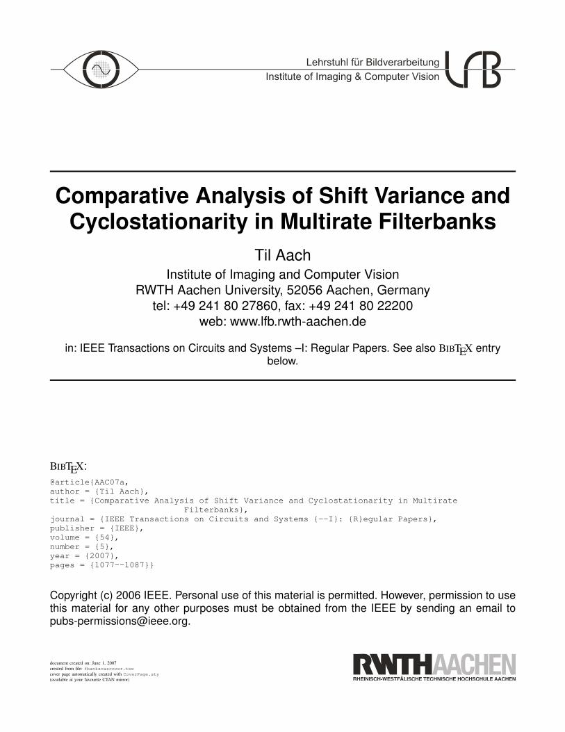
e, which also captures changesin the shape of the energy spectrum, for both channels of thetwo-channel filter banks. Since in image data shift variance isvisually most critical at fine detail structures such as lines andedges, the input signal here is s(n) = sgn(n) · exp{−0.9|n|},where sgn(n) = 1 for n ≥ 0, and sgn(n) = −1 for n < 0. Thisis a double-sided exponential impulse with a sign change at theorigin, which can be regarded as the gray level profile acrossan edge. The Haar filter now performs poorest, as expected,while the prcqf16 filters exhibit lowest shift variance. Amongthe linear phase filters, the biorthogonal 9/7 filters now performbest; in fact, they leave the biorthogonal 6/10 filters - whichled the field in Table III - far behind. The sha03-filter is nowalso relatively weak. Among the M-PRQM-filters, the filtersof length 4 outperform the others. To learn which spectralcomponents contribute strongest to shift variance, Figure 2shows the average of the normalized variance σ2
eN (ejω) in Eq.(20) over both filter bank channels of the Haar-, biorthogonal9/7-, biorthogonal 6/10- and the M-PRQMF4 filters. Evidently,the area under the variance average is largest for the Haarfilters. While for the M-PRQMF4 filters, the bandwidth ofthe averaged variance is comparable to that one of the Haarfilters, the maximum value is only about a third of that ofthe Haar filters, thus explaining the lower value for L2
e inTable V. For the longer biorthogonal filters, the bandwidthsof the variance averages are correspondingly narrower, withthe biorthogonal 9/7 filters reaching only a maximum of about0.12, thus explaining their low value for L2
e in Table V.
Table VI lists the values of L2e(i) for all eight channels of
DCT, MLT, and LOT driven by the same input signal. TheDCT is still weakest, but the performance of the MLT is nowrated better than that of the LOT.
We conclude our evaluations by an analysis of the nonsta-tionarity introduced into an AR(1)-random process (ρ = 0.9),as captured by the criterion K2
p . This criterion assesses thecyclic nonstationarity of the power spectrum, i.e, of the entirecorrelation structure, rather than only of the power. The resultsare listed in Tables VII and VIII. For the two-channel filter
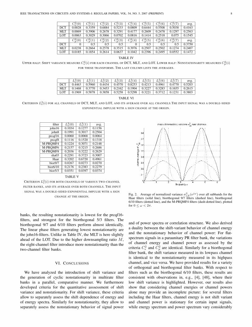
IEEE TRANSACTIONS ON CIRCUITS AND SYSTEMS–I: REGULAR PAPERS, VOL. 54, NO. 5, 2007 (PREPRINT) 8
C2e (0) C2
e (1) C2e (2) C2
e (3) C2e (4) C2
e (5) C2e (6) C2
e (7) avg.DCT 0.0028 0.3359 0.6884 0.5233 0.0809 0.6444 0.5508 0.5038 0.4163MLT 0.0069 0.3906 0.2678 0.3291 0.4177 0.2609 0.2478 0.1297 0.2563LOT 0.0063 0.3029 0.3066 0.0702 0.0816 0.1414 0.2518 0.075 0.1545
C2p(0) C2
p(1) C2p(2) C2
p(3) C2p(4) C2
p(5) C2p(6) C2
p(7) avg.DCT 0 0.5 0.5 0.5 0 0.5 0.5 0.5 0.3750MLT 0.0238 0.2664 0.2578 0.3515 0.3976 0.2507 0.2502 0.1274 0.2407LOT 0.0185 0.1854 0.2614 0.0637 0.1042 0.2396 0.2495 0.0552 0.1472
TABLE IVUPPER HALF: SHIFT VARIANCE MEASURE C2
e (i) FOR EACH CHANNEL OF DCT, MLT, AND LOT. LOWER HALF: NONSTATIONARITY MEASURES C2p(i)
FOR THESE TRANSFORMS. THE LAST COLUMN LISTS THE AVERAGES.
L2e(0) L2
e(1) L2e(2) L2
e(3) L2e(4) L2
e(5) L2e(6) L2
e(7) avg.DCT 0.4463 0.5960 0.4434 0.4570 0.8253 0.4213 0.4961 0.4770 0.5203MLT 0.1468 0.3770 0.3453 0.2162 0.1904 0.3227 0.3283 0.1655 0.2615LOT 0.1969 0.5878 0.3858 0.5258 0.5298 0.3221 0.3712 0.1231 0.3803
TABLE VICRITERION L2
e(i) FOR ALL CHANNELS OF DCT, MLT, AND LOT, AND ITS AVERAGE OVER ALL CHANNELS.THE INPUT SIGNAL WAS A DOUBLE-SIDED
EXPONENTIAL IMPULSE WITH A SIGN CHANGE AT THE ORIGIN.
filter L2e(0) L2
e(1) avg.john16 0.1034 0.1277 0.1156
john8 0.1991 0.3017 0.2504prcqf16 0.0060 0.0068 0.0064
prcqf8 0.1116 0.1520 0.1318M-PRQMF4 0.1224 0.3071 0.2148M-PRQMF6 0.2157 0.3215 0.2686M-PRQMF8 0.2036 0.3222 0.2629
sha03 0.2291 0.3723 0.3007Haar 0.3202 0.6720 0.4961
bior9/7 0.0267 0.0273 0.0270bior6/10 0.2176 0.2383 0.2279
bior5/3 0.0351 0.0397 0.0374
TABLE VCRITERION L2
e(i) FOR BOTH CHANNELS OF VARIOUS TWO-CHANNEL
FILTER BANKS, AND ITS AVERAGE OVER BOTH CHANNELS. THE INPUT
SIGNAL WAS A DOUBLE-SIDED EXPONENTIAL IMPULSE WITH A SIGN
CHANGE AT THE ORIGIN.
banks, the resulting nonstationarity is lowest for the prcqf16-filters, and strongest for the biorthogonal 5/3 filters. Thebiorthogonal 9/7 and 6/10 filters perform almost identically.The linear phase filters generating lowest nonstationarity arethe john16-filters. Unlike in Table IV, the MLT is here slightlyahead of the LOT. Due to the higher downsampling ratio M ,the eight-channel filter introduce more nonstationarity than thetwo-channel filter banks.
VI. CONCLUSIONS
We have analyzed the introduction of shift variance andthe generation of cyclic nonstationarity in multirate filterbanks in a parallel, comparative manner. We furthermoredeveloped criteria for the quantitative asssessment of shiftvariance and nonstationarity. For shift variance, these criteriaallow to separately assess the shift dependence of energy andof energy spectra. Similarly for nonstationarity, they allow toseparately assess the nonstationary behavior of signal power
Fig. 2. Average of normalized variance σ2eN (ejω) over all subbands for the
Haar filters (solid line), biorthogonal 9/7 filters (dashed line), biorthogonal6/10 filters (dotted line), and the M-PRQMF4 filters (dash-dotted line), plottedfor 0 ≤ ω < 2π.
and of power spectra or correlation structure. We also deriveda duality between the shift-variant behavior of channel energyand the nonstationary behavior of channel power: For flat-spectrum signals in a paraunitary PR filter bank, the variationsof channel energy and channel power as assessed by thecriteria C2
e and C2p are identical. Similarly for a biorthogonal
filter bank, the shift variance measured in its lowpass channelis identical to the nonstationarity measured in its highpasschannel, and vice versa. We have provided results for a varietyof orthogonal and biorthogonal filter banks. With respect tofilters such as the biorthogonal 6/10 filters, these results areconsistent with observations in, e.g., [4], [48], where theirlow shift variance is highlighted. However, our results alsoshow that considering channel energies or channel powersalone may provide an incomplete picture: for several filtersincluding the Haar filters, channel energy is not shift variantand channel power is stationary for certain input signals,while energy spectrum and power spectrum vary considerably

IEEE TRANSACTIONS ON CIRCUITS AND SYSTEMS–I: REGULAR PAPERS, VOL. 54, NO. 5, 2007 (PREPRINT) 9
K2p(0) K2
p(1) K2p(2) K2
p(3) K2p(4) K2
p(5) K2p(6) K2
p(7) avg.DCT 0.0574 1.3188 1.7589 1.7721 1.7803 1.6941 1.4695 0.6821 1.3166MLT 0.0293 0.7016 0.7006 0.6997 0.6993 0.6990 0.6968 0.2794 0.5632LOT 0.0389 0.7472 0.6843 0.7332 0.7079 0.8186 0.7875 0.3508 0.6085
TABLE VIIINONSTATIONARITY CRITERION K2
p(i) FOR ALL CHANNELS OF DCT, MLT, AND LOT, AND ITS AVERAGE OVER ALL CHANNELS. THE INPUT SIGNAL WAS
AN AR(1)-PROCESS.
filter K2p(0) K2
p(1) avg.john16 0.0003 0.1426 0.0714john8 0.0004 0.2887 0.1445
prcqf16 0.0002 0.1382 0.0692prcqf8 0.0003 0.2450 0.1226
M-PRQMF4: 0.0020 0.3539 0.1780M-PRQMF6: 0.0019 0.3110 0.1564M-PRQMF8: 0.0002 0.2946 0.1474
sha03 0.0002 0.3059 0.1531Haar 0.0047 0.3696 0.1872
bior9/7: 0.0001 0.3341 0.1671bior6/10: 0.0001 0.3231 0.1616
bior5/3: 0.0003 0.4592 0.2297
TABLE VIICRITERION K2
p(i) FOR BOTH CHANNELS OF VARIOUS TWO-CHANNEL
FILTER BANKS, AND ITS AVERAGE OVER BOTH CHANNELS. THE INPUT
SIGNAL WAS AN AR(1) RANDOM SIGNAL WITH ρ = 0.9.
over shift and position, respectively. We therefore believe thatour criteria which quantify the variations of energy spectraand power spectra provide, for applications such as imagefiltering and compression, a more realistic view. When thusanalyzing the shift variance of a test signal which can beregarded as representing the gray level profile across an edgein an image, the biorthogonal 9/7 filters outperformed the6/10 filters by a wide margin, while the Haar filter fell to thebottom of the list, as expected. A similar observation holds forthe introduction of nonstationarities: when examining channelpowers only, as done in Table III, the biorthogonal 6/10 filtersappear to outperform the 9/7 filters, while Table VII showsthat when considering the power spectrum, both filters behavein a similar way. In all cases, our criteria take the properties ofthe input signals into account in terms of their energy spectraand power spectra. The evaluation can thus be carried outspecifically for the signals where, e.g., shift variance is mostcritical, such as lines or edges in image data. This wouldallow to assess up to a certain degree the effects of, e.g., shiftvariance on the perceived subjective image quality, although noattempt was made to directly predict the visual image qualityas in [50] for static images.
VII. APPENDIX
We provide two approaches to derive Eq. (23), viz. a directone based on the polyphase decomposition of the interpolator[36], [37] shown in Fig. 3, and an alternative one using theeffects of interpolation on cyclic correlation functions andcyclic spectral densities described in [29].
Fig. 3. Polyphase decomposition of the interpolator.
With the kth polyphase component Gpk(z) of G(z) given by
Gpk(z) =
∞∑n=−∞
g(nM + k)z−n , k = 0, . . . ,M − 1 (52)
the filter G(z) can be written as [51]
G(z) =M−1∑k=0
z−kGpk(zM ) (53)
Vice versa, the polyphase components depend on the modula-tion vector of G(z) according to[
Gp0(z), z−1/MGp
1(z), . . . , z−(M−1)/MGpM−1(z)
]T
=
WM
gm(z1/M ) (54)
As is evident from Fig. 3, the ACS ryy(m,n) correspondsto the crosscorrelation sequence between the outputs of twopolyphase components of G(z) [52]. Since ryy(m,n) dependsperiodically on m, we set m = lM + i, i = 0, . . . ,M −1, andcalculate the ith power spectrum Ryy(i, z) by the transformryy(lM + i, n) ◦−• Ryy(i, z). Its polyphase representation is
Ryy(i, z) =M−1∑k=0
z−kRpyyk(i, zM ), i, k = 0, . . . ,M − 1
(55)The kth polyphase component Rp
yyk(i, z) is the crosscorrela-tion of the outputs of Gp
i (z) and Gp
(i+k)mod M(z):
Rpyyk(i, z) = Rxx(z)zb
i+kM cGp
i (z−1)Gp
(i+k)mod M(z) (56)
where bxc is the floor of x. Since here⌊i + k
M
⌋M = i + k − (i + k)mod M (57)

IEEE TRANSACTIONS ON CIRCUITS AND SYSTEMS–I: REGULAR PAPERS, VOL. 54, NO. 5, 2007 (PREPRINT) 10
and with Eqs. (53) and (55), we obtain
Ryy(i, z) = Rxx(zM )ziGpi (z
−M )G(z) (58)
Applying the ith component of Eq. (54) to the upsampled andmirrored polyphase component Gp
i (z−M ), and stacking the
results for i = 1, . . . ,M − 1 leads to Eq. (23).
Alternatively, we may start from the cyclic correlationfunction defined in [29, Eq. (21)], which, translated into ournotation, reads
rcyy(m,n) =
1M
M−1∑k=0
ryy(k, n)W−mk (59)
The cyclic spectral density function Syy(m, z) [29, Eq. (22)]is defined as the transform of rc
yy(m,n) with respect to n,yielding
Syy(m, z) =∞∑
n=−∞rcyy(m,n)z−n
=1M
M−1∑k=0
W−mk∞∑
n=−∞ryy(k, n)z−n (60)
Since∑
n ryy(k, n)z−n = Ryy(k, z), this can be written as
[Syy(0, z), . . . , Syy(M − 1, z)]T =WH
M[Ryy(0, z), . . . , Ryy(M − 1, z)]T (61)
Vice versa, we obtain
[Ryy(0, z), . . . , Ryy(M − 1, z)]T =W[Syy(0, z), . . . , Syy(M − 1, z)]T (62)
As derived in [29, Eq. (36)], the cyclic spectral density of theinterpolated signal obeys
Syy(m, z) =1M
G(z)Rxx(zM )G(z−1Wm) (63)
which, with Eq. (62), leads to Eq. (23).
REFERENCES
[1] R. E. Crochiere and L. R. Rabiner, “Interpolation and decimation ofdigital signals – a tutorial review,” Proceedings of the IEEE, vol. 69,no. 3, pp. 300–331, 1981.
[2] ——, Multirate Digital Signal Processing. Englewood Cliffs: Prentice-Hall, 1983.
[3] E. P. Simoncelli, W. T. Freeman, E. H. Adelson, and D. J. Heeger,“Shiftable multiscale transforms,” IEEE Transactions on InformationTheory, vol. 38, no. 2, pp. 587–607, 1992.
[4] J. D. Villasenor, B. Belzer, and J. Liao, “Wavelet filter evaluation forimage compression,” IEEE Transactions on Image Processing, vol. 4,no. 8, pp. 1053–1060, 1995.
[5] M. Antonini, M. Barlaud, P. Mathieu, and I. Daubechies, “Image codingusing wavelet transform,” IEEE Transactions on Image Processing,vol. 1, no. 2, pp. 205–230, 1992.
[6] A. Skodras, C. Christopoulos, and T. Ebrahimi, “The JPEG 2000 stillimage compression standard,” IEEE Signal Processing Magazine, vol.September, pp. 36–57, 2001.
[7] M. Stahl, T. Aach, and S. Dippel, “Digital radiography enhancement bynonlinear multiscale processing,” Medical Physics, vol. 27, no. 1, pp.56–65, 2000.
[8] C. M. Loeffler and C. S. Burrus, “Optimal design of periodically time-varying and multirate digital filters,” IEEE Transactions on Acoustics,Speech, and Signal Processing, vol. 32, no. 5, pp. 991–997, 1984.
[9] P. P. Vaidyanathan and S. K. Mitra, “Polyphase networks, block digitalfiltering, LPTV systems, and alias-free QMF banks: A unified approachbased on pseudocirculants,” IEEE Transactions on Acoustics, Speech,and Signal Processing, vol. 36, pp. 381–391, 1988.
[10] H. Xiong, T. Zhang, and Y. S. Moon, “A translation- and scale invariantadaptive wavelet transform,” IEEE Transactions on Image Processing,vol. 9, no. 12, pp. 2100–2108, 2000.
[11] J. Tian, “Comments on a translation- and scale-invariant adaptivewavelet transform,” IEEE Transactions on Image Processing, vol. 12,no. 9, pp. 1091–1093, 2003.
[12] J. Fan and A. Laine, Contrast Enhancement by Multiscale and NonlinearOperators. Boca Raton, FL: CRC Press, 1996, pp. 163–189.
[13] R. R. Coifman and D. L. Donoho, “Translation-invariant de-noising,” inWavelets and Statistics, A. Antoniades and G. Oppenheim, Eds. NewYork: Springer, 1995, pp. 125–150.
[14] J. Liang and T. W. Parks, “A translation-invariant wavelet representationwith applications,” IEEE Transactions on Signal Processing, vol. 44,no. 2, pp. 225–232, 1996.
[15] H. Malvar, “A modulated complex lapped transform and its applicationto audio processing,” in Proceedings ICASSP-99. Phoenix, AZ: IEEE,March 15–19 1999, pp. 1421–1424.
[16] I. W. Selesnick, R. G. Baraniuk, and N. G. Kingsbury, “The dual-treecomplex wavelet transform,” IEEE Signal Processing Magazine, vol.November, pp. 123–151, 2005.
[17] N. Kingsbury, “Complex wavelets for shift-invariant analysis and filter-ing of signals,” Applied and Computational Harmonic Analysis, vol. 10,pp. 234–253, 2001.
[18] D. Kunz and T. Aach, “Lapped directional transform: A new transformfor spectral image analysis,” in Proceedings ICASSP-99. Phoenix, AZ:IEEE, March 15–19 1999, pp. 3433–3436.
[19] T. Aach and D. Kunz, “A lapped directional transform for spectral imageanalysis and its application to restoration and enhancement,” SignalProcessing, vol. 80, no. 11, pp. 2347–2364, 2000.
[20] T. Aach, “Fourier, block and lapped transforms,” in Advances in Imagingand Electron Physics, P. W. Hawkes, Ed., vol. 128. San Diego:Academic Press, 2003, pp. 1–52.
[21] L. K. Shark and C. Yu, “Design of shift-invariant orthonormal waveletfilter banks via genetic algorithm,” Signal Processing, vol. 83, pp. 2579–2591, 2003.
[22] F. Mintzer and B. Liu, “Aliasing error in the design of multirate filters,”IEEE Transactions on Acoustics, Speech, and Signal Processing, vol. 26,pp. 76–88, 1978.
[23] V. P. Sathe and P. P. Vaidyanathan, “Effects of multirate systems on thestatistical properties of random signals,” IEEE Transactions on SignalProcessing, vol. 41, no. 1, pp. 131–146, 1993.
[24] A. K. Soman and P. P. Vaidyanathan, “Coding gain in paraunitaryanalysis/synthesis systems,” IEEE Transactions on Signal Processing,vol. 41, no. 5, pp. 1824–1835, 1993.
[25] U. Petersohn, N. J. Fliege, and H. Unger, “Exact analysis of aliasingeffects and non-stationary quantization noise in multirate systems,” inProceedings IEEE International Conference on Acoustics, Speech, andSignal Processing (ICASSP). Adelaide: IEEE, May 1994, pp. III–173–III–176.
[26] U. Petersohn, H. Unger, and W. Wardenga, “Beschreibung von Multirate-Systemen mittels Matrixkalkul,” AEU - International Journal of Elec-tronics and Communications, vol. 48, no. 1, pp. 34–41, 1994.
[27] U. Petersohn, H. Unger, and N. J. Fliege, “Exact deterministic andstochastic analysis of multirate systems with application to fractionalsampling rate conversion,” in IEEE International Symposium on Circuitsand Systems (ISCAS94), Vol. 2. Piscataway: IEEE, May 30 - June 21994, pp. 177–180.
[28] S. Ohno and H. Sakai, “Optimization of filter banks using cyclostation-ary spectral analysis,” in Proceedings IEEE International Conferenceon Acoustics, Speech, and Signal Processing (ICASSP). Detroit, MI:IEEE, May 1995, pp. 1292–1295.
[29] ——, “Optimization of filter banks using cyclostationary spectral anal-ysis,” IEEE Transactions on Signal Processing, vol. 44, no. 11, pp.2718–2725, 1996.
[30] A. Mertins, Signaltheorie. Stuttgart: Teubner, 1996.[31] S. Akkarakaran and P. P. Vaidyanathan, “Bifrequency and bispectrum
maps: A new look at multirate systems with stochastic inputs,” IEEETransactions on Signal Processing, vol. 48, no. 3, pp. 723–736, 2000.
[32] A. N. Akansu and H. Caglar, “A measure of aliasing energy in mul-tiresolution signal decomposition,” in Proceedings ICASSP-92. SanFrancisco, CA: IEEE, March 23–26 1992, pp. VI–621–VI–624.

IEEE TRANSACTIONS ON CIRCUITS AND SYSTEMS–I: REGULAR PAPERS, VOL. 54, NO. 5, 2007 (PREPRINT) 11
[33] L. Izzo and A. Napolitano, “Multirate processing of time series ex-hibiting higher order cyclostationarity,” IEEE Transactions on SignalProcessing, vol. 46, no. 2, pp. 429–439, 1998.
[34] B. Lal, S. D. Joshi, and R. K. P. Bhatt, “Second-order statisticalcharacterization of the filter banks and its elements,” IEEE Transactionson Signal Processing, vol. 47, no. 6, pp. 1745–1749, 1999.
[35] E. Serpedin, F. Panduru, I. Sari, and G. B. Giannakis, “Bibliography oncyclostationarity,” Signal Processing, vol. 85, pp. 2233–2303, 2005.
[36] A. N. Akansu and R. A. Haddad, Multiresolution Signal Decomposition.Boston: Academic Press, 2001.
[37] G. Strang and T. Nguyen, Wavelets and Filterbanks. Wellesley, MA,USA: Wellesley-Cambridge Press, 1997.
[38] T. Aach, “Shift variance and cyclostationarity in multiratefilter banks,” in 6th Nordic Signal Processing Symposium(NORSIG). Meripuisto, Espoo: IEEE, ISBN: 951-22-7065-X (print), 951-22-7031-5 (CD-ROM), 951-22-7032-3 (Web,http://www.wooster.hut.fi/publications/norsig2004), June 9–11 2004,pp. 85–88.
[39] ——, “Quantitative comparison of shift variance and cyclostationarity inmultirate filter banks,” in International Workshop on Spectral Methodsand Multirate Signal Processing (SMMSP), T. Saramaki, K. Egiazarian,and J. Astola, Eds. Vienna: TICSP Series, ISBN: 952-15-1229-6 (print),952-15-1241-5 (CD-ROM), Sept. 11 – 12 2004, pp. 7–14.
[40] G. D. Zivanovic and W. A. Gardner, “Degrees of cyclostationarity andtheir application to signal detection and estimation,” Signal Processing,vol. 22, pp. 287–297, 1991.
[41] W. A. Gardner, “Stationarizable random processes,” IEEE Transactionson Information Theory, vol. 24, no. 1, pp. 8–22, 1978.
[42] W. A. Gardner, A. Napolitano, and L. Paura, “Cyclostationarity: Half acentury of research,” Signal Processing, vol. 86, pp. 639–697, 2006.
[43] A. Papoulis, Probability, Random Variables, and Stochastic Processes(3rd ed.) New York: McGraw-Hill, 1991.
[44] J. R. Ohm, Multimedia Communication Technology. Berlin: SpringerVerlag, 2003.
[45] J. D. Johnston, “A filter family designed for use in quadrature mirrorfilter banks,” in Proc. ICASSP 1980. Piscataway: IEEE, 1980, pp.291–294.
[46] M. J. T. Smith and T. P. Barnwell III, “A procedure for designingexact reconstruction filter banks for tree-structured subband coders,” inProceedings IEEE International Conference on Acoustics, Speech, andSignal Processing (ICASSP). Denver: IEEE, March 1984, pp. 27.1.1–27.1.4.
[47] ——, “Exact reconstruction for tree-structured subband coders,” IEEETransactions on Acoustics, Speech, and Signal Processing, vol. 34, pp.434–441, 1986.
[48] J. Zan, M. O. Ahmad, and M. N. S. Swamy, “Comparison of waveletsfor multiresolution motion estimation,” IEEE Transactions on Circuitsand Systems for Video Technology, vol. 16, no. 3, pp. 439–446, 2006.
[49] H. S. Malvar, Signal Processing with Lapped Transforms. Norwood,MA: Artech House, 1992.
[50] Z. Wang and A. C. Bovik, “A universal image quality index,” IEEESignal Processing Letters, vol. 9, pp. 81–84, 2002.
[51] H. Johansson and O. Gustafsson, “Linear-Phase FIR Interpolation,Decimation and Mth-Band Filters Utilizing the Farrow Structure,” IEEETransactions on Circuits and Systems–I:Regular Papers, vol. 52, no. 10,pp. 2197–2207, 2005.
[52] T. Aach, “Shift variance in multiscale filtering,” in International Work-shop on Spectral Methods and Multirate Signal Processing (SMMSP),T. Saramaki, K. Egiazarian, and J. Astola, Eds. Barcelona, Spain:TICSP Series, ISBN: 952-15-1062-5, September 13–14 2003, pp. 23–30.
Til Aach (M 1994 – SM 2002) received his diploma and Doctoral degrees,both in EE, from RWTH Aachen University in 1987 and 1993, respectively.While working towards his Doctoral Degree, he was a research scientist withthe Institute for Communications Engineering, RWTH Aachen University,being in charge of several projects in image analysis, 3D-television andmedical image processing. From 1993 to 1998, he was with Philips ResearchLabs, Aachen, Germany, where he was responsible for several projects inmedical imaging, image processing and analysis. In 1996, he was also anindependent lecturer with the University of Magdeburg, Germany. In 1998,he was appointed a Full Professor and Director of the Institute for SignalProcessing, University of Luebeck. In 2004, he became Director of theInstitute of Imaging and Computer Vision, RWTH Aachen University. Hisresearch interests are in medical and industrial image processing, signalprocessing, pattern recognition, and computer vision. He has authored or co-authored over 160 papers, and received several awards, among these the awardof the German ”Informationstechnische Gesellschaft” (ITG/VDE), for a paperpublished in the IEEE Transactions on Image Processing in 1998. Dr. Aach isnamed as a co-inventor in about 20 patents. He is an Associate Editor of theIEEE Transactions on Image Processing, and was Technical Program Co-Chairfor the IEEE Southwest Symposium on Image Analysis and Interpretation(SSIAI) in 2000, 2002, 2004, and 2006. He is a member of the Bio-Imagingand Signal Processing Committee (BISP-TC) of the IEEE Signal ProcessingSociety.