COMPARATIVE STATISTICAL ANALYSIS OF TEST PARTS MANUFACTURED IN PRODUCTION

ENVIRONMENTS

David E. Gilsinn

U.S. Department of Commerce Technology Administration

Mathematical and Computational Sciences Division National Institute of Standards and Technology

Gaithersburg, MD 20899-8910

Alice V. Ling

AFRL/DEX 3550 Aberdeen Ave SE

Kirtland AFB, NM 87117-5776

NISTIR 6868

June 2002

1

Certain commercial software products are identified in this paper in order to adequately specify the computational procedures. Such identification does not imply recommendation or endorsement by the National Institute of Standards and Technology, nor does it imply that the software products identified are necessarily the best available for the purpose.

2

Abstract Estimating error uncertainties arising in parts produced on machine tools in production machine shops is not a well understood process. The current study details a process of estimating these error uncertainties. A part with significant features was defined and a vertical turning center was selected in a production shop to make multiple copies of the part. Machine tool error components were measured using a laser ball bar instrument. Twenty-one copies of the part were produced and measured on a coordinate measuring machine. A machine tool error model based on the measurements of the vertical turning center machine tool errors was developed. Uncertainty estimates of the errors in the working volume were calculated. From coordinate measuring machine data error uncertainties at points on the part were developed. Distances between hole centers were computed and uncertainty estimates of these lengths generated. Many of the hole centers were designed to fall along orthogonal lines. Uncertainty estimates were computed of the orthogonality of these lines. All of these estimated uncertainties were compared against uncertainties computed from the measured parts. The main conclusion of the work is that the Law of Propagation of Uncertainties can be used to estimate machining uncertainties and that predicted uncertainties can be related to actual part error uncertainties. Keywords: coordinate measuring machine, drilling, error uncertainties, laser ball bar, machine tools, machine tool errors, milling, Monte Carlo, propagation of uncertainty, vertical turning center.

3

Glossary ASME American Society of Mechanical Engineers CMM Coordinate Measuring Machine ISO International Organization for Standardization LBB Laser Ball Bar NC Numerical Controlled

4

Table of Contents

Abstract.............................................................................................................................. 3 Glossary ............................................................................................................................. 4 1.0 Introduction................................................................................................................ 7 2.0 Related Research......................................................................................................... 8 3.0 Parts Manufacturing and Machine Metrology ...................................................... 10

3.1 Milling Machine Specifications.............................................................................. 10 3.2 Parts Design ............................................................................................................ 10 3.3 Measuring the Vertical Machining Center.............................................................. 11

4.0 Part Uncertainty through Model Prediction .......................................................... 14 4.1 Kinematic Model for a Milling Machine ................................................................ 14 4.2 Regression Models for the Component Errors....................................................... 18 4.3 General Propagation of Uncertainties Using the Kinematic Model ....................... 23 4.4 Linear Distance Uncertainties................................................................................ 30 4.5 Orthogonality Uncertainties.................................................................................... 33 4.6 Circularity Uncertainties........................................................................................ 37

5.0 Part Uncertainties by Coordinate Measuring Machine Measurements .............. 40 5.1 Hole Center Location Uncertainties for Manufactured Part .................................. 40 5.2 Estimating the Uncertainty of a Machined Length Feature from CMM Measurements ............................................................................................................... 46 5.3 Estimating the Uncertainty of Machined Part Orthogonality from CMM Measurements ............................................................................................................... 48 5.4 Estimating the Uncertainty of a Machined Part Circularity from CMM Measurements ............................................................................................................... 49

6.0 Comparative Results................................................................................................ 51 6.1 Comparison of Hole Location Errors and Uncertainties........................................ 51 6.2 Comparison of Length Uncertainties ..................................................................... 52 6.3 Comparison of Orthogonality Uncertainties.......................................................... 53 6.4 Comparison of Circularity Uncertainties ............................................................... 53

7.0 Conclusions ............................................................................................................... 54 8.0 Acknowledgements .................................................................................................. 54 9.0 References ................................................................................................................. 55 APPENDIX A: Model Based Estimates of Point Error Variances and Confidence Intervals ........................................................................................................................... 57 APPENDIX B: Uncertainty Estimates for Hole Centers Based on CMM Measurements of Parts ................................................................................................... 63 APPENDIX C: Analysis of Variance for Selected Hole Centers ................................ 71 APPENDIX D: Derivation of the Variance of Length Equation ................................ 83 APPENDIX E: MACSYMA Program to Generate the Kinematic Model Error Equations ......................................................................................................................... 85 APPENDIX F: Circle Fit Algorithm ............................................................................. 87 APPENDIX G: Analysis of Variance for Computed Orthogonalities from CMM Measurements ................................................................................................................. 93 APPENDIX H: Analysis of Variance Tables for Circularities Computed from CMM Measurements ................................................................................................................. 94

5

6

1.0 Introduction1

In the production of machined parts a major problem can face a parts designer. Given a particular machine tool, how does one estimate beforehand the errors in features for the parts produced by that machine? Although there are general guides for reporting uncertainties in experiments (see ISO [1], Taylor and Kuyatt [2], American National Standards Institute [3]) there have been no published practical case studies on how to estimate uncertainties of errors of machined part features. Producing such a guide on the basis of case studies for a wide range of machine tools would be a large undertaking. This report can be regarded as an attempt at one chapter of such a guide. A project was defined in which a part was specified and given to a production machine shop with an order to make twenty one copies of the part on the same machine. A three-axis machining center on the shop floor was selected (See Figure 1). The part designed had drilled and milled holes and a circular slot (See Figure 2). The error components of the machine tool were measured multiple times by a laser ball bar (LBB). An error model of the machining center was developed and axis error uncertainties estimated by using the propagation of error formula from the ISO Guide [1]. An analytic formula was developed that could be used to estimate the variation in distance between features, such as hole centers. For orthogonal and circular features, Monte Carlo techniques had to be developed in order to estimate uncertainties. The parts themselves were measured on a coordinate measuring machine (CMM) and an analysis of variance technique was used to separate the measurement and manufacturing uncertainties of the measured hole centers and inner and outer radii of the circular slot. The various techniques employed are documented in this report in order to form a basis for estimating the uncertainties involved in producing parts on machine tools. The measurement of the machine tool (described in Section 3) was done by an instrument that measured machine tool errors at points on a plane above the parts production surface. Estimates of this height were not obtained at the time the machine tool error measurements were made. Therefore, the model as finally used in this report does not contain terms that include the errors due to this height difference. In future error measurements of similar machine tools these terms should be included. Since the object of this report was to develop a methodology, the authors feel that this oversight does not invalidate the overall procedures developed. A review of the related research literature is given in Section 2. Section 3 briefly describes the machine tool measurement procedure and the part design. Section 4 describes the kinematic model of a three axis machine tool along with the methods of estimating errors for point location, linear distances, orthogonalities and circularities. The uncertainty estimates for CMM measurements of the parts are given in Section 5. The comparative results are given in Section 6 with some final conclusions given in section 7.

1 The term “error” used in this report is used in the machining sense to refer to axis errors, e.g. linear axis errors, straightness errors, or orthogonality errors, rather than in the statistical sense.

7

2.0 Related Research Various authors discuss different aspects of the problem of machining uncertainties. Under a controlled set of experiments Wilhelm, Srinivasan and Farabaugh [4] have demonstrated that the measured behavior of the machine tool could be related to variations found in prismatic part features cut on that machine tool. The machining and metrology conditions were tightly controlled. A horizontal machining center was used. Parts, with features similar to those in the current study were cut. The results indicated that most part errors fell within two standard deviations of the machine errors. However, under uncontrolled conditions, a recent study by Chatterjee [5] has shown that there is a significant deviation in machine tool performance between static and operating conditions, where machine parameters are likely to vary due to cutting and thermal loads. Shin and Wei [6] developed a kinematic model for a multi-axis machine tool in order to predict deterministic errors. They added stochastic terms to the predicted errors and theoretically estimated the means and variances of the kinematic errors, but provide no experimental data comparison The inaccuracies that relate to drilling operations have been studied by a number of authors. These results, however, are in general experimental or analytic in nature and are not formulated in terms of uncertainties. Kaminski and Crafoord [7] state that drilling operations give rise to forces in the X, Y and Z directions as well as torque. They found that the tool deflects more under dynamic cutting conditions than under static simulated force loads. Lehtihet and Gunasena [8] use a simulation to show the influence of tolerance specification, size of the tolerance zone, hole size density, and production errors on the probability of producing an acceptable hole. Lee, Eman and Wu [9] discuss a mathematical model for drill wandering motion to explain the formation of odd-sided polygonal holes during initial penetration. Fujii, Marui and Ema [10, 11, 12] find that the drill point deflects along an elliptical orbit during whirling vibration. Magrab and Gilsinn [13] model a drill bit as a twisted Euler beam under axial loading that is clamped at both ends. The representative set of modes obtained exhibit a complex out-of-plane twisting-type motion that suggests a possible explanation for the out-of-roundness of certain drilled holes. In a work that relates to the current report Shen and Duffie [14, 15] develop an uncertainty analysis method that allows the modeling and computation of component error uncertainty sources that lead to coordinate transformation uncertainties. They show how uncertainties propagate in the homogeneous transformations of points, products of transformations and inverse transformations. They characterize the uncertainties associated with workpiece positions and orientations in terms of two components, a bias and a precision uncertainty component. They demonstrate that the bias and precision components can be propagated independently and combined to represent the uncertainties of the coordinate transformation relations. They validate the method by using Monte Carlo simulation (Bauer [16]).

8

Several recent papers relate measurement uncertainties in CMM measurements to the sampling strategy. Yau [17] proposes a general mathematical basis for representing vectorial tolerances. He develops a nonlinear, best-fit algorithm to evaluate vector tolerances for both analytic geometric elements and free-form surfaces. He then studies the uncertainty of the best-fit result caused by the sampling strategy and dimensional errors. Phillips et al. [18] examine the uncertainty of small circular features as a function of sampling strategy, i.e. the number and distribution of measurement points. They study the effect of measuring a circular feature using a three-point sampling strategy and show that the measurement uncertainty varies by four orders of magnitude as a function of the angular distribution of the measurement points.

9

3.0 Parts Manufacturing and Machine Metrology

3.1 Milling Machine Specifications The milling machine used to manufacture the test parts (Figure 1) is a three-axis vertical machining center with an X-axis (Longitudinal table) travel of 1020 mm (40 in), a Y-axis (Cross table) travel of 762 mm (30 in), and a Z-axis (Vertical head) travel of 560 mm (22 in). The programming resolution for all three axes is 0.001 mm (0.0001 in). The repeatability is reported by the machine manufacturer as 0.005 mm (0.0002 in) by the VDI 3441 method and +/- 0.0025 mm (+/- 0.0001 in) by the JIS 6330 method.

3.2 Parts Desig The part, shownmachining centeholes in the centThe “squared” ocenters. The largperpendicularitysquareness. Theperformance of

Figure 1: Three-Axis Machining Center

n

in Figure 2, was designed to illustrate several characteristics of the r. The holes around the outer edge have several purposes. First, drilled er were used to compute uncertainties in drilled hole center positioning. uter holes allowed comparison of milled hole centers to the drilled hole e square with 150mm sides was machined to check the orthogonality or of the machine’s X and Y axes. This property is sometimes called large internal circular features were cut in order to test the contouring the machine.

10

Figure 2: Test Part Specifications. Dimensions are in millimeters

3.3 Measuring the Vertical Machining Center The dimensional accuracy of the work piece is affected by the errors of the various positioning elements of the machine tool which contribute to the positioning accuracy of the cutting tool. Each machine element normally has one degree of freedom of nominal motion. But, there are six error components associated with each axis of motion. These six error components consist of three translations along, and three rotations about the three coordinate axes(roll, pitch and yaw). They are referred to as parametric errors, and in general are functions of axis position. For a three-axis machine tool there are twenty-one error components (six for each axis and three axis orthogonality errors).

11

ASME B5.54 [19] outlines techniques for performing parametric error measurements of machine tools using instruments such as laser interferometers, precision straight edges, capacitance gauges, and electronic levels. The use of these devices to perform error component measurements requires care and considerable time. Kakino, Ihara and Nakatsu [20] report the results of using a telescoping magnetic ball bar to measure circular motion errors of NC machines. They develop a formula that relates the radial displacement errors of the telescoping magnetic ball bar to the machine position error vector at a nominal point in the NC machine tool work volume. However, direct measurements of the spatial position of the tool are made feasible by using a metrology device that measures spatial positions by trilateration, called a laser ball bar (LBB) (see Figure 3). Trilateration is a technique in which a tetrahedron is formed with three base points (vertices) attached to the machine table, and the fourth attached to the tool holder. The three base points define a coordinate system. Simple geometric relationships allow the spatial coordinates of the fourth point or tool to be determined relative to this coordinate system. As the tool moves through space relative to the table, the lengths of the edges change causing the tetrahedron to deform. The LBB uses interferometry to measure the lengths of the tetrahedron edges and thus the tool position. The resulting measurement includes all effects which can cause positioning error: geometric, thermal and elastic. For a detailed discussion of the LBB and a comparison of the results of LBB measurements with ASME B5.54 measurements see Ziegert and Mize [21]. For a discussion of the use of a LBB in dynamic path measurements see Schmitz and Ziegert [22] and in modeling and predicting thermally induced errors see Srinivasa and Ziegert [23]. Various error components of the machine tool are measurable by the LBB. For example, when a single axis of a machine is actuated, the tool point is intended to move from the starting point to the ending point in a straight line. The distance between the starting and ending points should be exactly the displacement commanded. If it is not, then the machine is said to exhibit a linear displacement error. In general, the amount of the linear displacement error is a function of the axis position and direction of motion. Due to imperfections in the guideway system, the actual motion deviates from a perfect straight line. These deviations are termed straightness errors. The individual axes of a machine tool are constructed to provide axis motions which are perpendicular to each other. Due to imperfections in the machine construction, the actual motions of the axes are not exactly perpendicular. These errors are called axis alignment errors or squareness errors. Besides measuring displacement, straightness and squareness errors the LBB can measure the angular errors exhibited by the axes during motions. These are called roll, pitch and yaw. The measurement of these angular errors is accomplished by replacing the single tool socket with a fixture which holds three sockets, one of which is on the spindle centerline. The center socket is used to determine the linear displacement and straightness errors. Due to orientation changes, the displacement of the other two sockets will not be the same as the first. The LBB uses the difference in displacements of the three sockets to determine roll, pitch and yaw errors of the machine axis at each point along its travel.

12

The machine measurements were made by the following procedure. Five passes in both a forward and reverse direction were made in a large work volume that contained the smaller work volume enclosing the machined parts. This provided ten sets of data as a basis to model each of the error components of the milling machine. The LBB measured all twenty-one error components that define the errors for a three-axis mill. The data was used to develop regression models of the error components as functions of the positions along each machine axis. All five passes by the LBB were performed consecutively over a period of eight hours.

Figure 3: Laser Ball Bar Configuration

13

4.0 Part Uncertainty through Model Prediction Predicting part uncertainty by using a kinematic machine tool model requires a number of approximations. The first approximation assumes that the various error components combining to form a kinematic model of the machine tool errors enter in a linear fashion only. This is reasonable when the order of magnitude of the error components is examined. Any higher powers of the components become negligible. Second, the measurement of the machine error components indicate thermal drift of the errors between measurement repetitions as will be shown below. The authors recognize that the drift existed but could not control it during the measurement process. Thus for the purpose of this study the drift curves are treated as bona fide repeat curves and the resulting analysis will be assumed to be overly conservative. Finally, in order to estimate such quantities as circularity that are not defined in an analytical form, Monte Carlo simulation must be used in which an approximation to the distribution of the coverage factor for point uncertainties must be made. This will be discussed further below. In this section, a kinematic model of the machine tool, described in Section 3.1, will first be constructed. The error components entering into this kinematic model will then be shown to exhibit a linear trend over the workspace of the manufactured parts. A general analysis of point location uncertainties, based on this model, will then be given. Using the point uncertainty estimates an analytic method will be developed to estimate length uncertainties between feature points. Both analytic and Monte Carlo methods will then be used to estimate orthogonality uncertainties. Finally a Monte Carlo procedure will be used to estimate circularity uncertainty. 4.1 Kinematic Model for a Milling Machine The following notation will be used to describe the kinematic model for the three axis mill. 1. )(yxα - Angle between the X and Y axes 2. )(zxα - Angle between the X and Z axes 3. )(zyα - Angle between Y and Z axes 4. )(xxδ - X-Axis Scale Error 5. )( yyδ - Y-Axis Scale Error 6. )(zzδ - Z-Axis Scale Error 7. )(xyδ - Y Straightness of X 8. )(xzδ - Z Straightness of X 9. )(yxδ - X Straightness of Y 10. )(yzδ - Z Straightness of Y 11. )(zxδ - X Straightness of Z 12. )(zyδ - Y Straightness of Z 13. )(xxε - X Rotation of X (roll of X)

14

14. )(xyε - Y Rotation of X (pitch of X) )(x15. zε - Z Rotation of X (yaw of X)

16. )(yxε - X Rotation of Y (pitch of Y) of Y) - Y Rotation of Y (roll17. )yy (ε

)(yzε18. - Z Rotation of Y (yaw of Y) 19. )(zxε - X Rotation of Z (pitch of Z)

0.2 )(zyε - Y Rotation of Z (yaw of Z) 21. )(zzε - Z Rotation of Z (roll of Z) Three of the straightness errors must be modified to form generadue to the angular errors between axes. In particular

lized straightness errors

yyy xx ∆+ )()( αδ1. A generalized X-straightness error of Y motion is given by .

2. A generalized X-straightness error of Z motion is given by ∆ xx zzz + )()( αδ . 3. A generalized Y-straightness error of Z motion is given by zzz ∆yy + )()( αδ . In these formulas y∆ and z∆ represent incremental steps along the Y and Z axes. The construction of the kinematic model along the lines of Donmez [24] begins by assuming that a reference axis system is established by setting the part zero at the lower left corner of the part. The vertical, or Z, axis system is initialized vertically over the pazero but offset from it by a tool offset, 0z . To model a drilling operation three steps areperformed. First, the Y slide is moved forward, or in the negative Y direction. This sl

rt

ide

).

The motion of the Y slide with respect to the reference axis system is modeled by the product of an ideal motion matrix and the motion error matrix. This is given by

⎜⎜⎜⎛

−−−

⎟⎟⎟⎞

⎜⎜⎜⎛

=)()(1)(

)()()()(1010

0001yyy

dyyyyyy

T yxz

xxyz

y

δεεαδεε

(1)

The motion of the X slide with r led by the product of an ideal motion matrix and the motion error matrix. This is given by

carries the X slide along and holds the Z slide fixed. The second step is to move the X slide to the left and hold both the Y and Z slide fixed. Finally the Z slide is moved in adownward or negative Z direction to produce the drilled hole (See Figure 4 below

⎟⎟⎜⎜⎝

−⎟⎟⎠

⎜⎜⎝ 1000

)(1)()(10000100 yyy zxy δεε ⎟

⎟⎟

⎠

⎞

R

espect to the Y slide is mode

15

⎟⎟⎟⎟⎟

⎠

⎞⎜⎛ −

⎟⎞

⎜⎛ )()()(1001 xxxx xyz δεε

⎜⎜⎜⎜

⎝

−−

⎟⎟⎟⎟

⎠⎜⎜⎜⎜

⎝

=

1000)(1)()()()(1)(

100001000010

xxxxxx

Txxy

yxzx

y

δεεδεε

(2)

.

so

⎠

⎜⎜

⎝

⎛−

=

1000

010001

yTx . (3)

The motion of the Z slide with respect to the reference axis system is given by the product of the ideal motion matrix and the moti s

⎟

⎠

⎞

⎜⎜

⎜

⎝

⎛ −−

⎟⎟

⎟

⎠

⎞⎜

⎝

⎛

1000

)()()()(1

1000

0001 dzzzzz

zxy

xxyz αδεε

Z slide involves only an identity matrix as

⎟⎟

⎠

⎞

⎜⎜⎜⎜⎜

⎝

⎛

=

1000100

00100001

tzT

he matrix relating the work piece point relative to the reference axis, , is given by the matrix product

The work piece point with respect to the X slide involves only a translation matrixthat

⎟⎟⎟

⎜⎜⎜ 100 yw

⎟⎟⎞− x

on error matrix a

⎟⎟⎟⎟

⎜⎜−

−−⎟⎟

⎜⎜⎜⎜=

)(1)()()()()(1)(

1000010

zzzdzzzzz

zT yyxz

zR

δεεαδεε

. (4)

Finally the tool point with respect to the

⎟⎟⎟0

. (5)

w

RTT

wx

xy

yR

wR TTTT = (6)

16

and the matrix relating the tool tip to the reference axis, , is given by the matrix uct

. (7)

s, are given by

tRT

prod

tz

zR

tR TTT =

The error matrix relating the tool point to the workpiece, E, is then given by

wR

tR TTE 1−= . (8)

Using a symbol manipulator, such as MACSYMA, it is possible to compute the displacement errors of the work point with respect to the zero reference point (see

ppendix E). These errors , ignoring cross-products and higher-order termA

)()()()()()()()()( xzzzyyzxxyyyzyyE yxxxxzxyzx εααδδεδεε ++−−++++=

)()()()( yzxxxy )()()( xzzzzE xyyxyzyy εαδεδεδ −−+−= −+ , (9)

yxxyyy xyzxzE )()()( zxx zz)()()( δδεεδε −+−++−= .

erization rocedures outlined in the literature ASME B5.54 [19]. However, in this study the LBB ethods described in Section 3.3 were used. Although most of these errors are

repeatable, there is always a measurable amount of variation in the machine behavior due to various factors influencing the machine performance. These variations result in the variation of the estimates obtained by the kinematic equations given in equation (9) as well as the variation in the machined part dimensions and form. Since only planar errors are to be studied in this report any terms in equations (9) that involve a z coordinate value are dropped so that the final equations used to analyze the data are given by the following equations.

Equation (9) provides a formula for combining individual machine error components to estimate the resultant positioning error between the tool and the work piece. Individual rror components can be obtained using machine tool metrology characte

pm

)()()()()()()()(

xxxyEyyxxyyyyE

yzyy

xxzxzx

δεδαδεδε

+−=−+++=

(10)

In order to evaluate these formulas the first task was to develop equations for each of the components that relate the component errors to the coordinates x and y.

17

s

enter

4.2 In mesysrelthepooriforThmatwthecoomethememeerrma

Z - Slide

X - Slide Y - SlideR eference A xi

zz −0

A xis System for the Three A xis M achining C

Figure 4: Kinematic Model Axes Systems

Regression Models for the Component Errors

order to compare the results obtained from modeling machine tool errors with those asured on parts produced on the machine the strategy was to align the coordinate tems so that the origins and axes overlap. The data taken by the LBB was measured ative to the machine’s coordinate axis. The first step in modeling the data was to locate part origin for measurements within the machine coordinate system. This was the int used as the part origin when the parts were measured on a CMM. Although the part gin for machining was taken as the center of the part shown in Figure 2, the part origin measurements was taken as the lower left corner of the inner 150 by 150 mm square. e component error data on the machine tool was taken by the LBB relative to the chine coordinate system in steps of 25.4 mm in both the x and the y direction, with enty-five steps in the x direction and twenty-six steps in the y direction. For each of se points there were ten data values. The part origin for measurement in the machine rdinate system was located within one of these intervals for x and one for y. The an values of the ten data values for each of the error components were computed and ir values were interpolated to find the values of the components at the part origin for asurement. The data and the x and y scales were then shifted so that the part origin for asurement became the zero in the x and y coordinate system and the mean component ors at the part origin for measurement also became zero. This process aligned the on-chine measurements by the LBB with the part measurements made on the CMM.

18

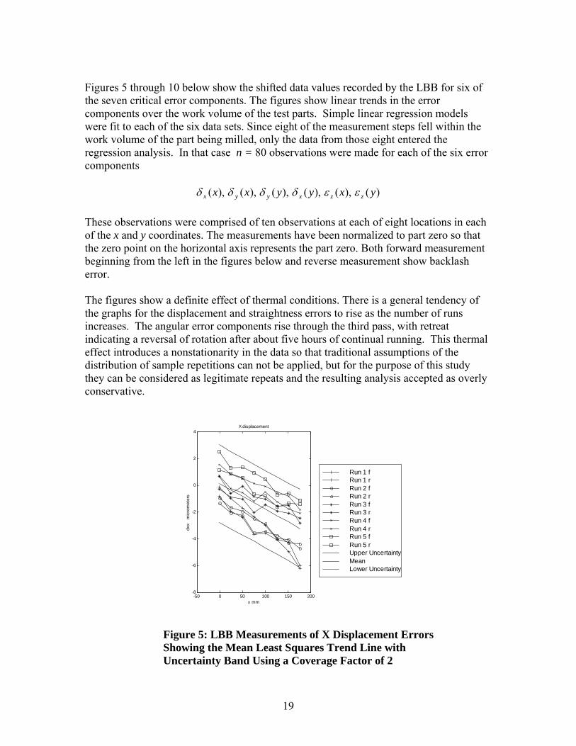
Figures 5 through 10 below show the shifted data values recorded by the LBB for six of the seven critical error components. The figures show linear trends in the error components over the work volume of the test parts. Simple linear regression models were fit to each of the six data sets. Since eight of the measurement steps fell within the work volume of the part being milled, only the data from those eight entered the regression analysis. In that case n = 80 observations were made for each of the six error components

)(),(),(),(),(),( yxyyxx zzxyyx εεδδδδ These observations were comprised of ten observations at each of eight locations in each of the x and y coordinates. The measurements have been normalized to part zero so that the zero point on the horizontal axis represents the part zero. Both forward measurement beginning from the left in the figures below and reverse measurement show backlash error. The figures show a definite effect of thermal conditions. There is a general tendency of the graphs for the displacement and straightness errors to rise as the number of runs increases. The angular error components rise through the third pass, with retreat indicating a reversal of rotation after about five hours of continual running. This thermal effect introduces a nonstationarity in the data so that traditional assumptions of the distribution of sample repetitions can not be applied, but for the purpose of this study they can be considered as legitimate repeats and the resulting analysis accepted as overly conservative.

-50 0 50 100 150 200-8

-6

-4

-2

0

2

4X displacement

x mm

dxx

mic

rom

eter

s

Run 1 fRun 1 rRun 2 fRun 2 rRun 3 fRun 3 rRun 4 fRun 4 rRun 5 fRun 5 rUpper UncertaintyMeanLower Uncertainty

Figure 5: LBB Measurements of X Displacement ErrorsShowing the Mean Least Squares Trend Line with Uncertainty Band Using a Coverage Factor of 2

19

-50 0 50 100 150 200-8

-6

-4

-2

0

2

4

6

8Y straightness of X

x mm

dyx

mic

rom

eter

s

Run 1 fRun 1 rRun 2 fRun 2 rRun 3 fRun 3 rRun 4 fRun 4 rRun 5 fRun 5 rUpper UncertaintyMeanLower Uncertainty

Figure 6: LBB Measurements of Y Straightness of X Errors Showing the Mean Least Squares Trend Line with Uncertainty Band Using a Coverage Factor of 2

FigS

-50 0 50 100 150 200-10

-8

-6

-4

-2

0

2

4

6

8

10Y displacement

y mm

dyy

mic

rom

eter

s

Run 1 fRun 1 rRun 2 fRun 2 rRun 3 fRun 3 rRun 4 fRun 4 rRun 5 fRun 5 rUpper UncertaintyMeanLower Uncertainty

ure 7: LBB Measurements of Y Displacement Errors howing the Mean Least Squares Trend Line with Uncertainty Band Using a Coverage Factor of 2

20

FigSh Ba

-50 0 50 100 150 200-5

0

5x 10-5 Z rotation of X

x mm

ezx

radi

ans

Run 1 fRun 1 rRun 2 fRun 2 rRun 3 fRun 3 rRun 4 fRun 4 rRun 5 fRun 5 rUpper UncertaintyMeanLower Uncertainty

Figure 9: LBB Measurements of Rotation About Z with X Motion Errors Showing the Mean Least Squares Trend Line with Uncertainty Band Using a Coverage Factor of 2

-50 0 50 100 150 200-6

-4

-2

0

2

4

6X straightness of Y

y mm

dxy

mic

rom

eter

s

Run 1 fRun 1 rRun 2 fRun 2 rRun 3 fRun 3 rRun 4 fRun 4 rRun 5 fRun 5 rUpper UncertaintyMeanLower Uncertainty

ure 8: LBB Measurements of Y Straightness of X Errors

owing the Mean Least Squares Trend Line with Uncertaintynd Using a Coverage Factor of 2

21

-50 0 50 100 150 200-4

-2

0

2

4x 10-5 Z rotation of Y

y mm

ezy

radi

ans

Run 1 fRun 1 rRun 2 fRun 2 rRun 3 fRun 3 rRun 4 fRun 4 rRun 5 fRun 5 rUpper UncertaintyMeanLower Uncertainty

Figure 10: LBB Measurements of Rotation About Z with Y Motion Errors Showing the Mean Least Squares Trend Line with Uncertainty Band Using a Coverage Factor of 2

The LBB measurement of the angular error between the x and y axes is independent of coordinate position. Table 1 gives the errors measured by the LBB in arc seconds and radians. The mean error in radians, estimated standard deviation and degrees of freedom are also given. These are used to estimate the confidence interval of a future observation of the angular error. Table 2 gives the slope and intercept values for the linear trend equations describing the error components shown in Figures 5 through 10.

Angular Error Between X and Y Axes Pass # Error (arcsec) Error(radians)

1 -6.99 -3.39-05 2 -6.43 -3.12E-05 3 -7.39 -3.58E-05 4 -6.76 -3.27E-05 5 -6.79 -3.29E-05 Mean -3.33E-05 Est. Std. Dev. 1.67E-06 Deg. Of Freedom 4

Table 1: LBB Measurements of the Angular Errors Between the X and Y axes

22

4.3 General Propagation o In order to estimate the unceassumption is made that theestimate the cross correlatio According to the Law of PrTaylor and Kuyatt [2], ColeE, such as those in equationuncorrelated

then the combined uncertainof the components, ignoring

u

Kinematic Error component Coefficients

Displacement Errors Slope Intercept Nondim. mm

-1.89E-05 1.04E-04 )(xxδ

-3.78E-06 5.16E-04 )(xyδ

-1.823E-05 1.38E-03 )(yyδ

)(yxδ -3.88E-06 8.55E-04

Rotational Errors Slope Intercept Nondim. radians

-2.87E-08 5.73E-06 )(xzε -5.62E-08 )(yzε 3.52E-06

X-Y Axes Angle Error Slope Intercept Nondim. radians

xyα 0.0000E+00 -3.33E-05

Table 2: Error Component Coefficients

f Uncertainties Using the Kinematic Model

rtainties associated with the resultant errors a preliminary individual error terms are uncorrelated since it is difficult to n of the different dimensional errors.

opagation of Uncertainty, outlined in the ISO Guide [1], man and Steele [25] and Wheeler and Ganji [26], if a variable (9), is a function of N stochastic components that are

),, N( 1fE γγ= (11)

ty of E, c , can be estimated in terms of the uncertainties second order terms, by

)(Eu

2f2 2( ) ( )

N

c iE u1i i

γγ

⎛≈ ⎜ ⎟∂∑ (12)

⎞∂

= ⎝ ⎠

23

The variances of the positioning errors in equation (9) can be computed from the propagation of uncertainties law by taking the appropriate partial derivatives as

))(())(())(())(())(()( 2222222

x

zuyuzxuxuxyuE yxyzyyc

ε

δεδεδ ++++=

rtainties ycxc uuEu one has to determine the ncertainties of individual error components using machine characterization data.

t

222222222 yuyxuxuyyuyuyyxEu αδεδε ++++=

he approximation here is that the components are taken to be uncorrelated. Since the measurement instrumentation used did not u us measurements of all omponent errors the assumption is necessary but simultaneous measurement is

r

ncertainties of the components can be estimated from their equations. The methods ery and Peck [27]. Since the component errors are modeled as

linear equations their regression equations take the form

))(()()())(())((

))(())(())(())(()(22222222

22222222

xuzuzuyzuxu

xuyyuyuzyuyEu

yxzxyxx

zxyzxc

εααδδ

εδεε

+++++

+++=

2u

))(()( 2222 uzuz xyzα ++ (13)

))((

))(())(())(())(())(()(2

222222222

zu

xuxuyxuxyuyuyEu

z

zxyzxzc

δ

δεεδε

+

++++=

To evaluate the unce )( zc EE ),(),(uFor completeness, equation (13) gives the error vector at any given point (x, y, z) in theworkspace, but since only uncertainties associated with planar features are of intereshere the uncertainty equations reduce to

))(())(())(()),(( 22222 xuxuxyuyxEu yzyyc

xxzxzxc

δεδ ++= (14)

))(())(())(())(())(()),((

Tallow sim ltaneo

cconside ed a standard in scientific work.

he uTare described in Montgom

εβ += Xy (15) where ε refers to the regression error, not to be mistaken for the rotational errors above, and

24

⎥⎦

⎢⎣ nε

⎥⎥⎥⎤

⎢⎡

⎤⎡ εε

β1

(16)

⎢⎢=⎥

⎦⎢⎣

=

⎥

⎦

⎤

⎢⎢⎢

⎣

⎡

=

⎥⎥⎥

⎦

⎤

⎢⎢⎢

⎣

⎡

=

nn x

x

X

y

y

y

εβ

β 2

2

1

22

1

,

1

1

,

servations. X is an n x 2 matrix of the regressor ariables.

⎥⎢⎥⎢ xy1

1

⎥⎥

In general, y is an n x 1 vector of obv β is a 2 x 1 vector whose components are: 1β the line intercept and 2β the line slope. ε is an n x 1 vector of random errors. The least squares estimator of β is given by the well kno wn formula

T 1)(ˆ −=β 7)

is

xy = 8)

yX T (1XX

Given a coordinate 1x , which could be along the x or y coordinate axis depending on theapproximate error component equation that is being evaluated, the predicted value computed as

β̂T (1ˆ where [ ]11 x= is the regressor variable. The regression model (15) can be used to predict a particular value of 0y corresponding to a specified level of regressor variable of 0x . In particular, let

xT

[ ]010 1 xxT = , then a point estimate of the future observation 0y is given by (18) as

β̂ˆ 00Txy = (19)

nder the conditions that the repetition samples and their standard errors satisfy certain

obability distribution requirements a confidence interval for this predicted ation is

Ustrict pr

bservo

))(1(ˆˆ

))(1(ˆˆ

01

02

00

01

02

0

xXXxkyy

xXXxkyTT

p

TTp

−

−

++≤≤

+−

σ

σ (20)

25

where pk is the coverage factor, taken here as 2=pk [ 2]. This interval is referred toa prediction interval for a future observation of 0y [27]. It is more conservative thaonfidence interval for the mean, but it is more meaningful for of parts production. For

as n the

cthe rest of this report the use of the term confidence interval will mean the predictioninterval. Also for the rest of this report the term 0

10

2 )(1(ˆ xXXx TT −+σ will be refeto as the standard uncertainty with the understanding that it is the standard error of a new

rred

observation given a value of the regressor variable. The expanded standard uncertainty is then

))(1(ˆ)( 01

02

0 xXXxxu TT −+σ (21) where

2=

2

ˆˆ 2

−−

=n

yXyy TTT βσ

ith y being the data used in (16).

igures 5 through 10 show the linear ower uncertainty bands based on the ) a coverage factor of 2. The

estimate an uncertainty terval for the next observation for a linear regression problem, can also be used to

estimate an uncertainty interval for the next sample of the angular error given in Table 1. lthough the angular error model is considered be a constant, the representation we select

e 1 and e X matrix given by . The parameter estimates are then given by

ase

(22)

w F equation fit to the data as well as the upper and

interval (20 with lcoefficients of the fitted linear equations are given in Table 2. At this point we will show how the formulas above, used toin

Ais given by equation (15) with the y vector given by the five angular errors in Tabl

[ ]T11111th

xyi

ixyTT YXXX ααβ === ∑

=

−5

1 1ˆequation (17). In this c1

,5)( . Thus the least squares

model in this case is the mean of the sam les. Furthermore p [ ]10 =x , so that

5)( 0

10 =− xXXx TT . The coverage factor will again be selected as 2. In this case, th

confidence interval for a future sample of the angular error between the x and y axes is given by

1 e

22 ˆ562ˆ

52 σαασα +≤≤− xyxyxy (23) 6

where

26

∑ ∑= =

−=5

1

5

1,

2,

2 )ˆ(41ˆ

i iixyixy αβασ (24)

which for the data in Table 1 is 2.88849e-12 radian squared. Therefore the uncertainty interval for a future angular error observation in radians is

595885.2570355.3 −−≤≤−− ee xyα (25) where the estimated standard deviation for a future sample is 1.86177e-6 radians. From the entries in Table 2 above one can substitute estimates into the component error equations of the form

1211

)(ˆ

)(ˆ

δ

ββδ

+=

+=

x

y

x

yy

xx

(26)

here the hat notation indicates that these equ ates for the les on the left. The degree of freedom of each of the first six estimates is seventy

ight, since there are eighty samples used to estimate the linear error component

3231

2221

)(ˆ)(ˆ

ββδ

ββδ

+=

+=y

yy

xx

4241 ββ

72

6261

5251

ˆ)(ˆ)(ˆ

βαββεββε

=+=+=

xy

z

z

yyxx

W ations are taken as estimvariabefunctions, and the degree of freedom of the last is four. The estimates of 2σ for each of the equations in (26) are given by

27

( )

( )

( )

( )

( )

( )

( ) ⎫⎩⎨⎧

−=

⎭⎬⎫⎧

−−=

⎭⎬⎫

⎩⎨⎧

−−=

⎭⎬⎫

⎩−

⎭⎬⎫

⎩−−

⎭⎬

⎩⎨

∑

∑

∑

=

=

=

=

5

1

2,

2

802

622

)

80

1

252

2)(

1

24241

22221

11211)(

41

)(1

)(781

78

)(78

78

iixy

iy

izx

iiix

iiy

iiixx

xy

z

y

x

yy

xx

y

xx

βασ

ββεσ

ββεσ

β

ββδ

α

ε

δ

(27)

in th

⎫⎧−−= ∑

8022 )(1 xx ββδσ

⎨⎧

−=

⎭⎬⎫

⎩⎨⎧

−−=

∑

∑=

=

802

)(

80

1

23231

2)(

1

)(1

)(781

y

iiiyy

i

x

y

y

yy

βδσ

ββδσ

δ

δ

⎨⎧

= ∑80

2)(

1xσδ

51 ii

⎩⎨

=161( 78 i

izzε

⎭⎬72

With these one can now estimate the variance of the variables on the left of (26) at a specific point ) e workspace. These are given by

,( 00 yx

⎪⎪⎭

⎪⎪⎬

⎫⎪⎪⎨

⎧−

+=

⎪⎪⎭

⎪⎪⎬

⎫

⎪⎪⎩

⎪⎪⎨

⎧

−

−+=

⎪⎪⎭

⎪⎪⎬

⎪⎪⎩

⎪⎪⎨

−

−+=

∑

∑

=

=

022

80

1

2

02)(0

2

80

1

2

02)(0

2

)(1))(ˆ(

)(

)(801))(ˆ(

)(

)(801))(ˆ(

ii

yy

ii

xy

yyyu

yy

yyyu

xx

xxxu

y

y

δ

δ

δ

σδ

σδ

σδ

⎪⎪⎩

−

⎫

⎪

⎪⎪⎬

⎫

⎪

⎪⎪⎨

−

−+=

∑

∑

=

80

1

2)(0

802

02)(0

2

)(80

)(

)(801))(ˆ(

ii

yx

i

xx

yy

xx

xxxu

x

xδσδ

⎧

⎧

⎪⎭⎪⎩ =1i

28

2 2 00 ( ) 80

2

1

2 2 00 ( ) 80

2

1

2 2

( )1ˆ( ( ))80 ( )

( )1ˆ( ( ))80 ( )

6ˆ( )5

z

z

xy

z x

ii

z y

ii

xy

x xu xx x

y yu yy y

u

ε

ε

α

ε σ

ε σ

α σ

=

=

⎧ ⎫⎪ ⎪−⎪ ⎪= +⎨ ⎬⎪ ⎪−⎪ ⎪⎩ ⎭⎧ ⎫⎪ ⎪−⎪ ⎪= +⎨ ⎬⎪ ⎪−⎪ ⎪⎩ ⎭

⎧ ⎫= ⎨ ⎬⎩ ⎭

∑

∑(28)

he c mbined standard uncertainties of the about the ean at a given gre or point are he ts

(ˆ((

(

))(ˆ())(ˆ())(ˆ()),(ˆ(

2220

20

220

2

022

002

022

0002

uux

uyu

xuyyuyuyyxEu

x

zxzxcp

δδ

εδε ++=

)

here the subscript cp indicates ut the mean at a oint . However, in order to estimate a confidence interval of a future error

T o estimated errors mre ss given by t square roo of

ˆ( ))( 0xy))(ˆ 0xzε +))( 0 xyy +)), 0 uy =ˆ(2 Eucp

)ˆ(α))(ˆ xδ +0x xy+ (29

w the combined standard uncertainty abo

),( 00 yxpresponse one must include the fact that the actual observed errors vary about their true means with estimated variances given by

2)(

2)(

20

2)(00

2

220

2)(

2)(

20

2)(

2)(

2000

2

)),((

)),((

xxyycm

xxyyxcm

yzy

xyxzxz

xyxEu

yyyyxEu

δεδ

αδεδε

σσσ

σσσσσ

++=

++++= (30)

here the subscript cm refers to the combined standard uncertainty about the mean

E . wThe combined standard uncertainty for a future error response is then computed by the

uare root of sq

)),(ˆ()),(()),((

)),(ˆ()),(()),((

002

002

002

002

002

002

yxEuyxEuyxEu

yxEuyxEuyxEu

ycpycmyco

xcpxcmxco

+=

+= (31)

here the subscript co refers to a future observation of the errors. These estimated ariances are given in tables A1 to A3 in Appendix A for the peripheral hole centers and r thirty-six evenly spaced points around the inner and outer rings of the circular slot on e part in Figure 2.

wvfoth

29

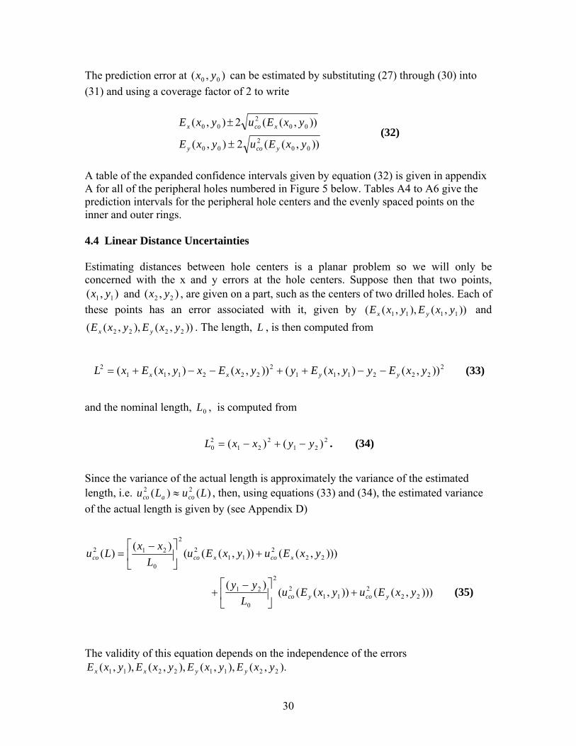
he prediction error at can be estimated by substituting (27) through (30) into 1) and using a coverage factor of 2 to write

),( 00 yxT(3

)),((2),(

)),((2),(

002

00

002

00

yxEuyxE

yxEuyxE

ycoy

xcox

±

± (32)

table of the expanded confidence intervals given by equation (32) is given in appendix for all of the peripheral holes numbered in Figure 5 below. Tables A4 to A6 give the rediction intervals for the peripheral hole centers and the evenly spaced points on the ner and outer rings.

4.4 Linear Distance Uncertainties Estimating distances between hole centers is a planar problem so we will only be concerned with the x and y errors at the hole centers. Suppose then that two points,

and , are given on a part, such as the centers of two drilled holes. Each of these points has an error associated with it, given by and

. The length,

AApin

),( 11 yx ),( 22 yx)),(),,(( 1111 yxEyxE yx

)),(),,(( 2222 yxEyxE yx L , is then computed from

(33)

and the nominal length, , is computed from

. (34)

Since the variance of the actual length is approximately the variance of the estimated length, i.e. , then, using equations (33) and (34), the estimated variance of the actual length is given by (see Appendix D)

2222111

2222111

2 )),(),(()),(),(( yxEyyxEyyxExyxExL yyxx −−++−−+=

0L

221

221

20 )()( yyxxL −+−=

)()( 22 LuLu coaco ≈

))),(()),((()(

))),(()),((()(

)(

222

112

2

0

21

222

112

2

0

212

yxEuyxEuL

yy

yxEuyxEuL

xxLu

ycoyco

xcoxcoco

+⎥⎦

⎤⎢⎣

⎡ −+

+⎥⎦

⎤⎢⎣

⎡ −=

(35)

The validity of this equation depends on the independence of the errors

).,(),,(),,(),,( 22112211 yxEyxEyxEyxE yyxx

30

Using equation (35) three length uncertainties are estimated. These uncertainties are ompared with uncertainties obtained from measuring the parts on a CMM. More

A1 in the

ion (33). The error uncertainties are also taken from Table A1 and e length uncertainty is computed by equation (35). The expanded prediction interval is

These tablescenters is le

cdistance uncertainties could be computed but the authors felt that the lengths chosenreflect the essential nature of the part uncertainties in general. The lengths chosen are the center-to-center lengths from hole number three (3) to hole number nine (9), from hole nine (9) to hole fifteen (15), and finally from hole three (3) to hole fifteen (15). The predicted point uncertainties for each of the three points are taken from Tableappendix, along with the nominal center locations. The estimated length is then computed using equatthcomputed using a coverage factor of two. The results are given in Tables 3 and 4 below.

HNu

H

Nu

X Axis ole mber

Nominal )(mm

Error )( mµ

Variance 2)( mµ

Uncertainty )( mµ

Expanded Uncertainty

)( mµ 3 10 1.15 6.86 2.62 5.24 9 10 5.04 20.96 4.58 9.16 15 140 2.07 20.83 4.56 9.12 Y Axis

ole mber

Nominal )(mm

Error )( mµ

Variance 2)( mµ

Uncertainty )( mµ

Expanded Uncertainty

)( mµ 3 10 1.63 22.60 4.75 9.50 9 140 -0.75 22.55 4.75 9.50 15 140 -1.43 31.23 5.59 11.18

Table 3: Line End-Point Uncertainties

Length Uncertainty Nominal Estimated Error Variance Uncertainty

)(mm )(mm )(mm

2)( mµ )( mµ Expanded

Uncertainty )( mµ

3 – 9 130 129.998 -0.002 45.1 6.72 13.44 9 – 15 130 129.997 -0.003 41.8 6.47 12.94 3 - 15 183.848 183.846 -0.002 40.7 6.38 12.76

Table 4: Line Length Uncertainties

are consistent in that the uncertainties squared of the lengths between hole ss than the sum of the squares of the component uncertainties.

31

3

4

5

6

8

7 17

9 10 11 12 13 14 15

16

18

20

212224 2326 25

19

130 mm

130 mm

10 mm

(0,0)

32

4.5 Orthogonality Uncertainties If the part shown in Figure 2 and Figure 11 were ideal then the line through holes 9 through 15 would lie at right angles to the lines through holes 9 through 3. However, real arts seldom, if ever, satisfy this property. In general there is a small angular difference

between the actual angle that the two line for a right angle. This is termed an rthogonality error. Each copy of the same part will have a slightly different

of these orthogonality errors is the pic of this section.

ince each of the hole centers has a point uncertainty this means that there is error in both

es a problem with finding the best ne through the centers of the holes. Assume that we are given points

and we wish to find he lssumption behind the least squares estimation of coefficients is that the linear first order

ps m and

oorthogonality error. The uncertainty in the distributionto

Sthe x and y positions of the center. This fact introducli

),(,),,( 11 NN yxyx t east squares line through the points. The amodel can be written as εββ ++= xy 10 where the ε term represents the deviation in

8]. d errors in variables.

this report we will use two different approaches. The first is a technique suggested by oleman and Steele[25] in which the uncertainties in the least squares coefficients

the y variable from the line. Thus all of the error in the approximation is assumed to be relegated to the y variable and the x variable is assumed to have no error. The problem of fitting equations to data in which both variables are subject to error, see e.g. Mandel [2The relevant methods are calle In

10 ,ββ Care connected to the uncertainties in the data points themselves. The second is a Monte

arlo approach in which the x and y distributions of the hole centers are sampled a large umber of times, horizontal and vertical lines fit to the resulting points, and angular ifferences from right angles computed. The uncertainty in this large sample of

the

Cndorthogonality errors can then be computed. In the first of the two methods (Coleman and Steele[25] ) the assumption is made thatpoints ),(,),,( 11 NN yxyx are given data points and the usual least squares estimates of the slope and intercept are given by

∑ ∑

∑∑∑∑

∑∑

====

==

⎞⎛

−=

⎟⎠

⎜⎝

⎛−

N N

N

iii

N

ii

N

ii

N

ii

ii

ii

yxxyx

xxN

21111

2

0

11

2

)()(

)(

β

(36)

∑ ∑ ∑

= =

= =

⎟⎠

⎜⎝

−

−=

i iii

NN

N

i

N

i

N

iiii

xxN

yxyxN

1 1

2

1 11

)(

β

Each of these coefficients can be thought of as functions of the data points so that

=

⎞i

21

33

),,,,,(),,,,,(

1100

1111

NN

NN

yyxxyyxx

ββββ

==

7) (3

Using the propagation of uncertainties formula one gets

∑ ∑

∑∑

= =

==

⎟⎟⎠

⎞⎜⎜⎝

⎛∂∂

+⎟⎟⎠

⎞⎜⎜⎝

⎛∂∂

=

⎟⎟⎠

⎞⎜⎜⎝

⎛∂∂

+⎟⎟⎠

⎞⎜⎜⎝

⎛∂∂

=

N

i

N

iiiyco

iiixco

ico

N

iiiyco

iiixco

N

i ico

yxEuy

yxEux

u

yxEuy

yxEux

u

1 1

22

022

00

2

1

22

122

1

11

2

))ˆ,ˆ(())ˆ,ˆ(()(

))ˆ,ˆ(())ˆ,ˆ(()(

βββ

βββ

(38)

error term of the rm

where we assume that each point is the sum of a nominal point plus an fo

)ˆ,ˆ(ˆ)ˆ,ˆ(ˆ

iiyii

iixii

yxEyyyxExx

+=+=

(39)

o get the uncertainties on the right hand side of (38) one uses the fact that

(40)

he orthogonality errors only require computing slope differences so that we only need to ompute the partial derivatives of the slope

T

))ˆ,ˆ(())ˆ,ˆ(ˆ()(

))ˆ,ˆ(())ˆ,ˆ(ˆ()(222

222

iiycoiiyicoico

iixcoiixicoico

yxEuyxEyuyu

yxEuyxExuxu

=+=

=+=

T

1β . These are given by c

2

1 1= = ⎠⎝i i

2

11

2

1

2

1

2

11 1 111

2

1

2

1

)(

)(

2)(

∑ ∑

∑

∑ ∑

∑∑ ∑ ∑∑∑ ∑

=

= =

== = === =

⎟⎞

⎜⎛

−

−=

⎥⎥⎦

⎤

⎢⎢⎣

⎡⎟⎠

⎞⎜⎝

⎛−

⎥⎦

⎤⎢⎣

⎡−⎥

⎦

⎤⎢⎣

⎡−−⎥

⎦

⎤⎢⎣

⎡−

⎥⎥⎦

⎤

⎢⎢⎣

⎡⎟⎠

⎞⎜⎝

⎛−

=

N N

ii

N

iik

k

N

i

N

iii

N

iik

N

i

N

i

N

iiiii

N

iik

N

i

N

iii

k

xxN

xNx

y

xxN

xNxyxyxNyNyxxN

x

β

β

(41)

rs

∂∂

∂∂

where ),( ii yx are given by (39). For the case of the vertical lines between hole centeone fits x against y and the roles of x and y in (41) reverse. The fitted horizontal and vertical lines will take the form

34

yxxy

vv

hh

,1,0

,1,0

ββββ

+=

+= (42)

Since the slopes are small and the tangent of a small angle is approximately the angle in radians one may equate the slopes with angles. But in order to preserve the sign convention with respect to the horizontal axis the slope of the vertical line in (42) must have its sign changed. Thus the two angles are given by

v

h

,12

,11

βθβθ−=

= (43)

and the difference, or orthogonality error, is given by

12 θθθ −=∆ (44) The uncertainty of the orthogonality is computed as

)()()()()( ,12

,12

12

22

hcovcocococo uuuuu ββθθθ +=+= (45)

here the last two uncertainties are computed using (38), (39) and (41).

2 ∆

The uncertainty of the orthogonality of the part was estimated using the horizontal holes 3, 26, 25, 24, 23, 22, 21 and the vertical holes 3, 4, 5, 6, 7, 8, 9 shown in Figure 5. No xpansion factor is used here.

A secon Monte

andardere thesignaere co

w

e

arandomstwdw

Analytic Estimate of Orthogonality Standard Uncertainty -5.10 11.09

Table 5: Analytic Estimates of Orthogonality Uncertainty in arc sec. The Uncertainty is not Expanded.

d approach to estimating the unc tain he orthogonality error is by means of Carlo simulation. To generate an orthogonality error angle twenty eight (28)

sa m a normal distribution with zero mean and unit deviation, since there were fourteen holes used to estimate orthogonality. There

en two random numbers associated with each hole, one for x and one for y, ted b . For each of the fourteen hole centers the following simulated points mputed

er ty of t

mples were selected fro

y yx RR ,

))ˆ,ˆ(()ˆ,ˆ(ˆ))ˆ,ˆ(()ˆ,ˆ(ˆyxEuRyxEyyyxEuRyxExx

ycoyy

xcoxx

++=++=

(46)

35

The horizontal and vertical least squares lines through the appropriate new hole centers

and vertical line combination were computed using (36) for the horizontal lines and the appropriate equations for thevertical lines. For each horizontal θ∆ was computed using

2) through (44). This process was repeated a large number of times, M, and the estimated standard deviation (4

σ̂ was computed. The prediction uncertainty was given by

⎟⎠⎞

⎜⎝⎛ +=∆

Muco

11ˆ)( 22 σθ (47)

he results from a simulation with M =1000 is given in the table below.

T The figure b

Bin

Cou

nts

Mean Orthogonality (arc sec)

Sample Standard Deviation (arc sec)

Standard Uncertainty (arc sec)

-4.68 11.02 11.03

Table 6: Orthogonality Uncertainty. The Uncertainty is not Expanded.

elow shows the distribution of the orthogonality samples.

-50 -40 -30 -20 -10 0 10 20 300

20

40

60

80

100

120Distribution of Orthogonality

Orthogonality (arc sec)

Figure 12: Distribution of the Orthogonalities for 1000 samples.

36

4.6 Circularity Uncertainties

ISO 230-4 [29] on circular tests for numerically controlled machine tools circular eviation is defined as the minimum radial separation of two concentric circles nveloping the path produced by the machine tool when programmed to move on the ircular path defined by its diameter (or radius), the position of its center and its rientation in the working zone. Optionally the circular deviation may be evaluated as the aximum radial range around the least squares circle. The first definition requires

omputing the minimum zone circles which can be formulated as a linearly constrained ptimization problem. The algorithm for computing the minimum zone circles is fficiently complex that, for practical purposes, the approach of selecting a least squares

ircle provides a tool that can be used in a Monte Carlo simulation to estimate the ncertainty of the circular deviation or circularity. The algorithm used here to fit the least uares circle is the Marquardt-Levenberg, based on an algorithm described in Nash [30]. discussion of the algorithm is given in Appendix F.

order to compare the estimated uncertainties with the results of measurements of the arts on a CMM, the same nominal points on the inner and outer walls of the circular slot ature of the parts were selected. There were thirty six points (36) selected on each wall

round the circular profile. This meant ten degrees between each nominal point. The ominal points were designated as . The estimated circularity and its ncertainty were calculated by a Monte Carlo simulation. First one thousand random umbers were sampled for each point from a normal distribution with a mean of zero and andard deviation of one and designated for

IndecomcosucusqA Inpfea

)ˆ,ˆ(,),ˆ,ˆ( 363611 yxyxnun

)1000,(,),1,( iRiR xx 36,,1=ist . Another ne thousand samples were selected from the same distribution for each point and were esignated for

od )1000,(,),1,( iRiR yy 36,,1=i . For each group of thirty-six random umbers, new x and y points were generated using (46). Thus, for the kth Monte Carlo mulation from one to a thousand the new points were computed as

nsi

))ˆ,ˆ((),()ˆ,ˆ(ˆ))ˆ,ˆ((),()ˆ,ˆ(ˆ

iiycoyiiyii

iixcoxiixii

yxEukiRyxEyyyxEukiRyxExx

++=++=

(48)

ext, a least squares circle was fit through these points using the Marquardt-Levenberg onlinear optimization procedure. This produced the best fit center for the data. The istance from this point to each of the thirty-six new points was computed and the ircularity was computed as the maximum of these distances minus the minimum. This rocedure was repeated a thousand times. The distribution of the circularities is given in e histograms in Figures 13 and 14. The corresponding prediction uncertainty for a

future sample is given by

Nndcpth

)1000

11(ˆ)( 22 += σCuco (49)

where is the sample variance

2σ̂

37

sing a coverage factor of two the prediction interval for the inner circular slot edge,

.

Mean Circularity (mm) Standard Uncertainty (mm) 0.0179 0.0031

Table 7: Circularity Uncertainty for Inner Circle Feature

Ubased on the simulation results is

0241.0)0031.0(20179.0)0031.0(20179.00117.0 =+≤≤−= c (50)

T Using a coveragebased on the simu

0118.0 = These results are the range (50) or

Mean Circularity (mm) Standard Uncertainty (mm)

0.0180 0.0031

able 8: Circularity Uncertainty for Outer Circle Feature

factor of two the prediction interval for the outer circular slot edge, lation results is

0242.0)0031.0(20180.0)0031.0(20180.0 =+≤≤− c (51)

in millimeters. The next sample taken would be expected to fall with(51)

in with a 95% confidence.

38

0.005 0.01 0.015 0.02 0.025 0.03 0.0350

10

20

30

40

50

60

70

80

90

100Distribution of Circularity for inner Path of Circular Slot

Bin

Cou

nts

Circularity (mm)

Figure 13: Histogram of the Sampled Circularity for 1000 Samples

of the Inner Circle Feature Circularity.

0.01 0.015 0.02 0.025 0.03 0.0350

10

20

30

40

50

60

70

80

90

100Distribution of Circularity for Outer Path of Circular Slot

Circularity (mm)

Bin

Cou

nts

ularity for 1000 Samples Figure 14: Histogram of the Sampled Circof the Outer Circle Feature Circularity.

39

5.0 Part Uncerta Measuring Machine Measurements

wenty one parts made according to Figure 2 were measured on a CMM. The following oint locations were measured: the hole center locations for the drilled portion of the

holes, the hole centers of the milled portion of the holes, thirty six evenly spaced points g edge of the oute spaced points

ge of the inner circle. Fiv ese points were peats were performed on the other

arts.

i

he following notation will be used to estimate the manufactured part uncertainties: 1. - Measured Hole Location Errors along the X and Y axes.

inties by Coordinate

Tp

alon the r ring of the circular slot and thirty six evenly along the ed e repeat measurements for each of thmade on part numbers one through four, while two rep In this section an analysis of variance procedure is explained that isolates the manufacturing error from the coordinate measuring machine error. Manufacturing andmeasurement uncertaint es are estimated. The analysis of variance procedure is applied to estimate the uncertainties of the locations of the hole centers for both drilled and milled holes as well as to estimate the orthogonality and circularity. An estimate of theuncertainty of the distance between features is also developed 5.1 Hole Center Location Uncertainties for Manufactured Part T

my

mx EE ,

2. ay

ax EE , - Actual Hole Location Errors along the X and Y axes.

3. yx ηη , - Hole Location Measurement Process Errors along the X and Y axes.

The main assumption made here is that the actual hole location errors due to the anufacturing process and the measurement process errors are uncorrelated. Therefore,

be added to estimate the variances of the measured ole location errors.

yy

am VEVEV η+=

l relative to ppose that the

easured error variance is a good approximation of the actual manufactured hole error variance. That is if then a

x VEV ilarly for y.

or each machined part, the errors in hole positions are measured by the CMM relative to

uare shown in Figure 2. The X and Y locations of the centers of each drilled and milled hole on each of the twenty-one parts were measured a multiple number of times.

mtheir corresponding variances canh

)()()( amxxx

VEVEV η+= (10)

)()()(

y

If the variances of the measurement process errors can be shown to be smalthe variances of the measured hole location errors then it is reasonable to sum

)()( mxx EVV <<η )( m

xE≈ and sim)(

Fa part coordinate system located at the lower left corner of the inner 150 mm X 150 mmsq

40

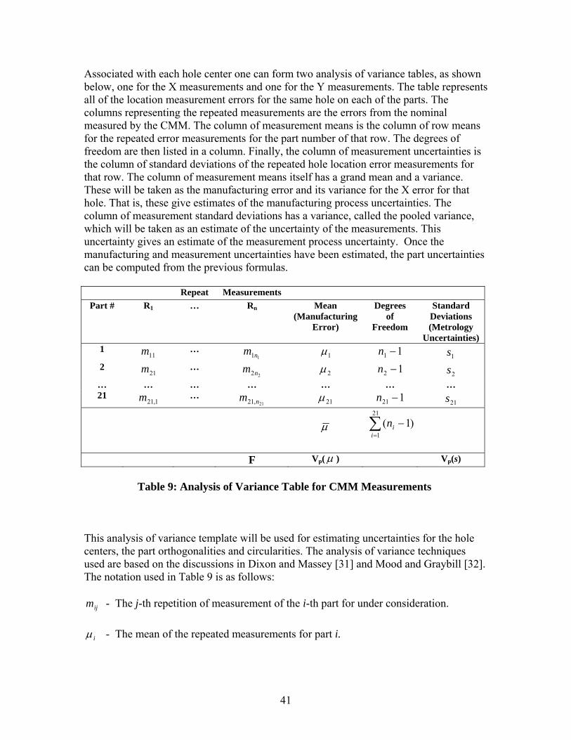
Associated with each hole center one can form two analysis of variance tables, as shown

ns

he X error for that ole. That is, these give estimates of the manufacturing process uncertainties. The

estimate of the measurement process uncertainty. Once the anufacturing and measurement uncertainties have been estimated, the part uncertainties

This analysis of variance template will be used for estimating uncertainties for the hole centers, the part orthogonalities and circularities. The analysis of variance techniques used are based on the discussions in Dixon and Massey [31] and Mood and Graybill [32]. The notation used in Table 9 is as follows:

- The j-th repetition of measurement of the i-th part for under consideration.

below, one for the X measurements and one for the Y measurements. The table represents all of the location measurement errors for the same hole on each of the parts. The columns representing the repeated measurements are the errors from the nominal measured by the CMM. The column of measurement means is the column of row meafor the repeated error measurements for the part number of that row. The degrees of freedom are then listed in a column. Finally, the column of measurement uncertainties isthe column of standard deviations of the repeated hole location error measurements for that row. The column of measurement means itself has a grand mean and a variance. These will be taken as the manufacturing error and its variance for t

hcolumn of measurement standard deviations has a variance, called the pooled variance, which will be taken as an estimate of the uncertainty of the measurements. This uncertainty gives anmcan be computed from the previous formulas.

Repeat Measurements Part # R1 … Rn Mean

(Manufacturing Error)

Degrees of

Freedom

Standard Deviations (Metrology

Uncertainties) 1

11m … 11nm 1µ 11 −n 1s

2 21m …

22nm 2µ 12 −n s2 … … … … … … … 21

1,21m … 21,21 nm 21µ 121 −n 21s

∑=

−21

µ 1

)1(i

in

F Vp(µ ) Vp(s)

Table 9: Analysis of Variance Table for CMM Measurements

ijm

iµ - The mean of the repeated measurements for part i.

41

i - Standard Deviation of the repeated measurements for part i.

f - Total degrees of freedom.

p

s

∑=

−=21

1

)1(i

ind

(µ ) = 121

))((21

1

2

−

−∑=i

iin µµV - Estimate of the between part uncertainty.

p(s) = df

sn ii∑ − 2)1(V - Estimate of the within part uncertainty.

he ratio T )(/)( sVVF pp µ= is used to determine whether there is a significant difference

etween the two variance estimates (Montgomery and Peck [27], Chapter 2). For the ases of concern here, the test value for the F distribution at the 95% level with 20 egrees of freedom for

bcd ( )pV µ and 34 (i.e., 54 – 20) degrees of freedom for , since

ere are 54 totpproximately r

s the value above is an interpolation erred to Dixon and Massey 1] for a discussion of the analysis of variance for a one-way fixed effects classification odel.

t this point we need to introduce some further terminology. Let

(14)

e the total number of measurements over all the parts. Then the pooled mean, called the ean manufacturing error or grand mean, is given by

( )pV sth al measurements for each hole center, over all of the parts, is

1.89. Since most tables give values for 30 and 40 degrees of freedom fo. The reader is ref

a( )pV

[3m A

∑=

=21

1iinN

bm

N

ni

ii∑==

21

1µ

µ . (15)

he pooled standard deviation is T

)(sVs pp = (16)

n estimate of the standard uncertain A

ty of the grand mean is given by

42

N

su p= (17)

n estimate of the uncertainty of a future measurement sample is given by A

pf sN

u ⎟⎟⎠

⎞⎜⎜⎝

⎛+=

11 (18)

he corresponding expanded uncertainty of a future measurement will then be taken as T

ff uU 2= (19)

ummary tables of these quantities are given in Tables B1 through B4 in Appendix B for e measurement uncertainties of each of the peripheral holes for all of the parts. Tables 1 and B2 summarize the results for the X and Y measurements of the drilled holes and ables B3 and B4 summarize the results for the X and Y measurements of the milled oles. B o n f the t the ole ce ird olumn gives the uncertainty of a new m the hole center and finally the urth column gives an expanded uncertainty of this measurement.

ables B.5 through B.8 in Appendix B give a summary of the analysis of variance tables r all of the manufacturing errors of all holes for all of the parts. The hole numbers are

iven in Figure 11.

igures 15a and 15b below show the mean measured errors for the centers of the three rilled holes numbered 3, 9 and 15. These three holes represent the lower left hole, the pper left hole and the upper right hole respectively. These holes will be used in the next ction to evaluate uncertainties in length measurements. The first thing that can be noted

bout the measurements is that part 13 shows a significant negative x mean error for all ree drilled holes compared to the other parts. This appears to be reflected in the y mean

rrors for that part also. These plots reflect the numbers in tables C1, C2, C5, C6, C9 and 10 in Appendix C. Notice also the significant center location errors for parts 3, 19, 21 nd 27 (whose stamped part blank was mistakenly machined in place of part 20).

igure 16b shows sharp error difference for the Y measurements of milled holes 9 and 15 n parts 6 and 21. This is confirmed by looking at tables C8 and C12.

SthBTh oth the drilled and milled holes have the same nominal centers. The first c

ables gives the estimates in micrometers of the mean manufacturing error of nter. The second column gives the standard uncertainties of the error. The th

easurement of

lumohcfo Tfog FduseatheCa Fo

43

5 10 15 20 25-0.06

-0.04

-0.02

0

0.02

0.04

0.06Hole 3Hole 9Hole 15

Figure 15a: Mean X Errors for the Centers of the Dr

Vertical Axis represents Errors in mm. Horizontal Axis representPart Numbers.

illed Holes. s

5 10 15 20 25-0.06

-0.04

-0.02

0

0.02

0.04

0.06Hole 3Hole 9Hole 15

Figure15b: Mean Y Errors for the Centers of the Drilled. Horizontal Axis re

Holes. presents Vertical Axis represents Errors in mm

Part Numbers.

44

5 10 15 20 25

0

0.005

0.01

0.015

0.02

0.025

0.03

0.035 Hole 3Hole 9Hole 15

f the Milled Holes. The

Vertical Axis represents Errors in mm. The Horizontal Axis represents Figure 16a: Mean X Errors for the Centers o

Part Numbers.

5 10 15 20 25

0

0.035

0.005

0.01

0.015

0.02

0.025

0.03

Hole 3Hole 9Hole 15

Figure 16b: Mean Y Errors for the Centers of the Milled Holes. The Vertical Axis represents Errors in mm. The Horizontal Axis represents

Part Numbers.

45

5.2 Estimating the Uncertainty of a Machined Length Feature from CMM M ement

he lengths and uncertainties of these lengths will be examined for the distances between errors and

mean (

easur s

Tthree holes on the parts machined. The summary statistics of the measured

10 and 11. The error uncertainties are given for the three hole center features in Tablesvariance estimates given in Tables 10 and 11 are computed as the pooled variance of the

)(µpV ). The measurement variance estimates are computed as the pooled variance

square roots of the varian timates. Table 10 gives the results for the rilled hole centers for feature holes 3, 9, and 15, while Table 11 gives the results for the

me. For the purpose of this study, then, the measurement mean for each hole will be

of the estimated measurement variances ( )(sVp ). The uncertainty estimates are omputed as the c ce es

dmilled square hole centers for the same feature holes. The tables give the nominal coordinates of the hole centers, relative to the part origin in the lower left corner. Since the measurement of the feature errors are composed of both manufacturing and CMM measurement errors, the tables then give the manufacturing error, variance and uncertainty of the part feature as well as the CMM measurement variance and uncertainty for each feature. The data show that the CMM measurement uncertainties are one to two orders of magnitude less than the manufacturing uncertainties. This verifies the assumption that )()( x

mx EVV <<η , and similarly for the Y errors. Thus measured

variances of hole location errors and variances of actual location errors can taken as the sataken as an estimate of the manufacturing error for that hole and the measurement uncertainty in Table 9 above will be taken as the measurement uncertainty for each hole.

Summary Drilled Hole Statistics

X Axis Location CMM Measurement

Hole Nominal Error Variance Uncertainty Variance Uncertainty

Number )(mm )( mµ 2)( mµ )( mµ 2)( mµ )( mµ

3 10 2.73 641 25.3 1.10 1.05

9 10 4.99 511 22.61 1.19 1.09

15 140 -4.52 566 23.79 0.710 0.843

Y Axis Location CMM Measurement

Hole Nominal Error Variance Uncertainty Variance Uncertainty

Number )(mm )( mµ 2)( mµ )( mµ 2)( mµ )( mµ

3 10 2.70 1371 37.03 0.743 0.862

9 140 2.70 1925 43.87 0.678 0.823 15 140 2.70 2410 49.09 0.982 0.991

Table 10: tainty S ri , and 15. The Uncert t E ertai

Uncerainties are no

tatistics for Dxpanded Unc

lled Holes 3, 9nties.

46

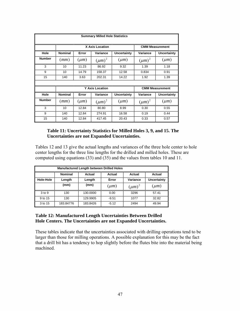
Summary Milled Hole Statistics

X Axis Location CMM Measurement

Hole Nominal Error Variance Uncertainty Variance Uncertainty

Number )(mm )( mµ 2)( mµ )( mµ 2)( mµ )( mµ

3 10 11.23 86.92 9.32 1.39 1.18

9 10 14.79 158.37 12.58 0.834 0.91 15 140 3.63 202.31 14.22 1.92 1.39

Y Axis Location CMM Measurement

Hole Nominal Error Variance Uncertainty Variance Uncertainty

Number )(mm )( mµ 2)( mµ )( mµ 2)( mµ )( mµ

3 10 12.84 80.80 8.99 0.30 0.55

9 140 12.84 274.91 16.58 0.19 0.44 15 140 12.84 417.45 20.43 0.33 0.57

Table 11: Uncertainty Statistics for Milled Holes 3, 9, and 15. The Uncertainties are not Expanded Uncertainties. Tables 12 and 13 give the actual lengths and variances of the three hole center to hole center lengths for the three line lengths for the drilled and milled holes. These are computed using equations (33) and (35) and the values from tables 10 and 11.

Manufactured Length between Drilled Holes

Nominal Actual Actual Actual Actual Hole-Hole Length Length Error Variance Uncertainty

(mm) (mm) )( mµ 2)( mµ )( mµ

3 to 9 130 130.0000 0.00 3296 57.41

9 to 15 130 129.9905 -9.51 1077 32.82 3 to 15 183.84776 183.8426 -5.12 2494 49.94

Table 1 en ties B d

ole Cente e Un erta nded nties.

hese tables indicate that the uncertainties associated w operations tend to be rger than ing op sib iat a d y tly b for toachined.

2: Manufactured Lrs. Th c

gth Uncertaininties are not Expa

etween Drille UncertaiH

T ith drilling la those for mill

rill bit has a tendencerations. A pos

to hop sligh ele explanation for the the flutes bite in

s may be the fact the material being th

m

47

Manufactured Length between Milled Hole Centers

Nominal Actual Actual Actual Actual

Hole-Hole Length Length Error Variance Uncertainty (mm) (mm) )( mµ 2)( mµ )( mµ

3 to 9 130 130.0000 0.00 355.71 18.86

9 to 15 130 129.9888 -11.16 360.68 18.99 3 to 15 183.84776 183.8424 -5.40 393.74 19.84

Table 13: Manufactured Length Uncertainties Between Milled Hole

enters. The Uncertainties are not Expanded Uncertainties.

centers form lines parallel to the edges of the parts. Two nominally orthogonal lines of holes (the bottom row and left side row) were selected to estimate the uncertainties in the orthogonality of these two lines of holes. All of the twenty-one parts had the milled hole centers measured on a high precision CMM with repeated measurements of each part. The first four parts had five repeated center measurements and the rest of the parts had two repeated measurements. The procedure of estimating orthogonality was as follows: For the centers of the holes along the Y-axis a least squares fit of the line form y = mx + b was made for each of the repetitions for each of the parts. This produced a table of slope values for m. Since the deviation of m from 0 was small the values of m could be used as angle estimates since for small angles tan(a) ≈ a in radians and m is the tangent of the slope angle. Next the vertical line of hole centers was fit with an equation of the form x = my + b. The sign of the resulting slope had to be reversed and then it could be added to the horizontal slope to determine the orthogonality error. This calculation is similar to that leading to equations (42) to (44). Table G1 was produced. The grand mean represents the mean of all of the orthogonality estimates, including repetitions and is properly weighted by the degrees of freedom. The uncertainty of the means is the manufacturing uncertainty and the uncertainty of the standard deviations is the CMM measurement uncertainty. We will summarize the results in Table 14 below. The error means and variances come from Table G1, while the other entries are based on the formulas in Section 5.1.

C

5.3 Estimating the Uncertainty of Machined Part Orthogonality from CMM Measurements From Tables B5 through B8 it is clear that the center locations of milled holes have lower manufacturing errors. The peripheral milled hole centers were selected as points to be used for estimating orthogonality. The milled holes were designed to have their nominal

48

iance oan be consid

O

irty seven p

Note that the the var

MaErro

PooDevMa

Erro

TablMeas

c 5.4 EstimatinMeasuremen

n each of th2). The inner milled clockwthe CMM andrepeated measBased on the could be comthTables 15 andNote that ther

Mean nufacturing

VaMa

Uncertainties

r sec)(arc Error sec)(arc 2sec)(arc

riance of the nufacturing

Variance of the Metrology

2

-1.059 80.285 8.768 led Standard iation of the nufacturing r sec)(arc

Pooled Standard Uncertainty

sec)(arc

Uncertainty of a Future

Orthogonality Estimate

sec)(arc

Expanded Uncertainty of

a Future Orthogonality

Estimate sec)(arc

8.96 1.22 9.05 18.10

e 14: Summary of the Orthogonality Statistics from CMM urements

f the manufacturing error so that the measured and manufacturing variances ered approximately equal.

part

n

t radius of the oints. From these calculations Table H1 and Table H2 were prepared.

variance of the metrology uncertainties is an order of magnitude less than

g the Uncertainty of a Machined Part Circularity from CMM ts

e s a circular slot was milled with an inner and outer radius (see Figuresurface of the slot was milled counterclockwise and the outer surface was ise. Thirty seven equally space poi ts on each surface were measured on the resulting radii from the best fit center were reported. Again five urements were made on the first four parts and two on each of the others.

thirty seven measured points on each surface a value for the circularity puted as the difference between the largest and the smalles

16 below summarize the statistics. Terminology is given in Section 5.1.e are fifty four circularity estimates for each table.

Mean Manufacturing Error )( mµ

Variance of the Manufacturing Errors

2)( mµ

Variance of the Metrology

Uncertainties 2)( mµ

20.986 7.378 3.130 Pooled Standard Deviation of the

Manufacturing Errors )( mµ

Pooled Standard Uncertainty )( mµ

Uncertainty of a New Circularity Estimate

)( mµ

Expanded Uncertainty of a New Circularity Estimate

)( mµ 2.716 0.370 2.743 5.486

Table 15: Summary Statistics for Inner Circle of Slot

49

Note that the variance of measurements of the inner wall of the circular wall is less thanthe variance of the manufacturing errors in Table 15. Several factors could have accounted for this. The inner and outer walls of the circular slot were cut in oppo

Mean Manufacturing Error )( mµ

Variance of the Manufacturing Errors

2)( mµ

Variance of the Metrology

Uncertainties 2)( mµ

26.018 35.836 2.556 Pooled Standard Deviation of the

Expanded Uncertainty of a New Circularity Estimate

Uncertainty of a New Circularity Estimate

Pooled StandaUncertainty ( m

rd )µ

)( mµ Manufacturing Errors )( mµ )( mµ

5.986 0.815 6.046 12.092

Table 16: Summary Statistics for Outer Circle of Slot

site irections. Direction of cut may have had an effect in leaving small debris. The inner

walls m ht not ha hows the measurement v n o ude e v anufacturing errors.

dig ve been cleaned sufficiently. Table 16 s

ariance to be a rder of magnit less than th ariance of the m

50

6.0 Comparative Results

6.1 Comparison of Hole Location Errors and Uncertainties When we compare the predicted errors computed from LBB measurements forperipheral holes given in Table A1, the mean errors measured by the CMM shown in Tables B1 through B4 tend to be larger. The manufacturing uncertainties for a given feature measurement s

the

hown in Tables B5 through B8 are significantly greater than those redicted by the LBB measurements. These latter are the square roots of the variances

be

ter they

easurements falls between 6.81 and 20.96 . For the y-errors the predicted . For the parts measured by the CMM

m rs

7

inties) from the model predictions is there some multiple that could be used to estimate conservatively the actual manufacturing variances (uncertainties) of the parts for the given machining center? In order to estimate this relation we can start by considering the ratios between the lower limits of the manufacturing error variances and the model predicted variances. For the drilled holes the lower limit ratio for x-machine errors (511.40/6.81) gives 75.1. The upper limit ratio (1279.0/20.96) gives 61.0. For the milled holes the lower x-machine error ratio is 12.76 and the upper ratio is 10.1. For the y-machine error variances for the drilled holes the lower limit ratio (1310.32/22.37) is 58.57 and the upper ratio (2489.11) is 79.55. Similarly for the milled holes the lower ratio is 3.52 and the upper is 13.66. These ratios are not immediately revealing. However, since we are looking for relations between the uncertainties which are the square roots of the variances we wish to examine

pgiven in the last two columns of Table A1. The signs of the errors for both the predicted errors and the measured errors tend to consistent for the drilled holes. This does not mean that they are all the same but that theyin general cluster in the same groups. For the x-machine errors the signs clusnegatively between holes twenty-five and fourteen, whereas for the y-machine errors cluster between nineteen and six. The consistency does not seem to hold for the milled holes. From Table A1, the range of the predicted variances x-errors based upon the LBB

2mµ 2mµmvariances fall between 22.37 2mµ and 31.29 mµ 2

the variances are significantly higher. These are given in column two of Tables B5 through B8. For the x-machine errors for the drilled holes the error variances fall between 511.40 2mµ and 1279.0 2mµ . For the illed holes the center x-machine errorange from 86.92 2 to 211.42 2mµ . The y-machine error variances tend to be larger. For the drilled holes the y-machine error variances fall between 1310.32 2mµ and 2489.11 2mµ . For the milled holes the y-machine error variances fall between 78.7

2mµ and 427.54 2mµ . We can note here that the y-machine error variances are in general greater than the x-machine error variances in both the model prediction and CMM measurement cases. A question arises at this point. If we only knew the variances (uncerta

mµ

51

the square roots of these ratios. Taking square roots we can see that for the x-errors in the drilled case the ratios fall betwee ereas in the milled case they fall etween 3.17 and 3.57. Similarly in the y-error cases they fall between 7.65 and 8,91 for

f we

.2 Comparison of Length Uncertainties

r le shows the upper and lower bounds for the

ncertainty range. The uncertainties for the milled hole center-to-center lengths are also

Drilled Hole Expanded Uncertainty Range

n 7.81 and 8.67 whbthe drilled holes and 1.88 and 3.70 for the milled holes. These ranges suggest that, iwished to estimate the actual machining operation uncertainties for the machining center used, then, to be conservative, we could take an uncertainty multiple of 9 for drilling operations and 4 for milling operations. 6 The uncertainties associated with the three hole center-to-center lengths are summarizedin Table 17 below. The drilled hole uncertainty range is computed from Table 12 by expanding the uncertainties in that table. The mean length error is obtained by subtracting the nominal length from the actual length given in the table. Twice the length uncertainty given in Table 12 was then added and subtracted from the mean length erroto give the uncertainty range. The tabugiven in Table 17. These have been computed by expanding uncertainty data given in Table 4. The average ratio of the drilled hole-to-hole range to the comparable modelrange is 7.2 while the average for the similar ratios for the milled holes is 2.96.

Center-to-Center Lower Uncertainty Mean Length Upper Uncertainty Range

Lines Bound )( mµ Error )( mµ Bound )( mµ )( mµ

3 to 9 -114.82 0.00 114.82 229.64

9 to 15 -75.15 -9.51 56.13 131.28 3 to 15 -105.00 -5.12 94.76 199.76

Milled Hole Expanded Uncertainty Range

Center-to-Center Lower Uncertainty Mean Length Upper Uncertainty Range Width

Lines Bound )( mµ Error )( mµ Bound )( mµ )( mµ

3 to 9 -37.72 0.00 37.72 75.44

9 to 15 -49.14 82 75.96 -11.16 26.3 to 15 -45.08 -5.40 34.28 79.36

Expanded Uncertainty Estimates Based on LBB Machine Metrology

Center-to-Center Lower Uncertainty Mean Length Upper Uncertainty Range Width

Lines Bound )( mµ Error )( mµ Bound )( mµ )( mµ

3 to 9 -15 -2 11 26 9 to 15 -16 -3 10 26 3 to 15 -15 -1.8 11 26

Table 17: A Comparison of the Upper and Lower Expanded Uncertainty Limits for the Hole-to-Hole Lengths based on the CMM Measurements and the Model Estimates Based on the LBB Machine Measurements.

52

The next observation relates to the ratio of the measured length uncertainties to the computed length uncertainties. The Srinivasan and Farabaugh [4]

owed that the position errors of the test part holes fell in general within two standard eviations of the measured machine errors. Their work however was conducted under

app standard deviations. The parts in this study were not milled under lts of this

studman measured

con

exp e analytic and Monte Carlo t

mea onality error from the this

cas predicted the orthogonality error but did produce the same

Not

the

mac 17.9

work of Wilhelm,shdcontrolled laboratory conditions. In terms of expanded uncertainties this would allow for

roximately fourcontrolled conditions, but under ordinary shop environment conditions. The resu

y suggest that for the machining center used the potential length errors of ufactured parts could fall as far away as seven standard deviations of the

machine errors for drilled holes and three for milled holes. This conclusion can only be sidered tentative.

6.3 Comparison of Orthogonality Uncertainties.

The mean orthogonality error from Tables 5 and 6 is –4.89 arc sec and the averageanded uncertainty is 22.12 arc sec. These are based on th

me hods of estimating orthogonality from the machine tool model and LBB surements. From Table 14 the mean manufacturing orthog

CMM measurements is –1.06 arc sec with an expanded uncertainty of 18.1 arc sec. Ine the model estimates over-

direction of error. Similarly the model results over-predicted the expanded uncertainty. e that both the errors and uncertainties were both discrepant by about 4 arc sec.

6.4 Comparison of Circularity Uncertainties

The first circularity errors and uncertainties to be considered are those predicted byhine model. The mean circularity error for the inner circle feature from Table 7 is mµ while the expanded uncertainty if 6.2 . For the outer circle Table 8 shows mµ

these to be 18.1 mµ and 6.2 mµ respectively. The results from the CMM measured ts show that for the inner circle the mean circularity error is 20.99 mpar µ and the

expanded uncertainty is 5.49 mµ . For the outer circle the circularity error is 26.02 mµ and the expanded uncertainty is 12.09 mµ . From these results it appears that the values

the model are cfrom loser to the CMM measurements for the inner circle, at least in terms

be h terclockwise of uncertainty. There is one fact that might have some relevance here although it would

ard to determine the actual effect. The inner circle was milled in a counfashion, whereas the outer circle was milled in a clockwise fashion.

53

7.0 Conclusions

foreesti se only apply to the individual machine being studied, however it would

dete

loc equate kinematic model of ere the

law in cases where there are no e law to

be aapp mate the uncertainties.

Set ent errors was cumbersome, but it did provide measurements for all of the components

s in a reas mponent measurement.

Alt ut a larger number of parts, the twenty-one parts that .

Thi ng a procedure to estimate the uncertainties of

sma parts and then developing an uncertainty table

des by the fact that

cha

ledgements

The s of the NIST staff who participated in

mea instrumental in running the vertical machining center during the measurement of the machine with the laser ball bar but also during the machining of the parts. M. Alkan Donmez supervised the overall project and provide invaluable consulting on machine metrology. Richard Rhorer played an important part in the early design of the experiment and part design. Johannes A. Soons designed the final part selected, provided machine tool programming and metrology consultation.

There are a number of conclusions that can be drawn from this study. The first and most is that machining uncertainties can be estimated for production machines. These mates of cour

be interesting to do a parallel study on a production machine in the same family andrmine whether there are any commonalities.

The law of Propagation of Uncertainties provides a means of estimating both point ation and length uncertainties when combined with an ad

the machine tool under study. There are uncertainties, such as for circularity, wh cannot be applied directly. These uncertainties occur

clearly understood functional relationships between quantities that would allow thpplied. In these cases some form of simulation or Monte Carlo technique must be lied to esti

ting up and calibrating the particular LBB for measuring the machine tool compon

necessary to model the machine tool. It was possible to take all of the measurementonably short time without changing fixtures for each co

hough the original plan was to c

were finally produced provided adequate data to estimate uncertainties in the machinings makes it feasible to consider developi

a new machine tool by performing a machine tool characterization, cutting a reasonably ll set of reference parts, measuring the

for that machine. This table could be used by a part designer as a tool in any parts igned for production on that machine. This possibility is reinforced

there seem to be computable relations between uncertainties estimated from racterization and the actual production uncertainties.

8.0 Acknow

authors wish to thank the many member

various ways to make this project a success. Bruce R. Borchardt did the painstaking surements of the manufactured parts on a CMM. Robert R. Clary, a machinist, was

54

9.0 References

in

te, “American National Standard for Expressing Uncertainty – U.S. Guide to the Expression of Uncertainty in Measurement”, ANSI/NCSL Z540-2-1997.

. W l rom Machine Tool Performance Measur n CIR

1. International Organization for Standardization, Guide to the Expression of Uncertainty

Measurement. 2. Taylor, B. N., Kuyatt, C. E., “Guidelines for Evaluating and Expressing the

Uncertainty of NIST Measurement Results”, NIST Technical Note 1297, NationalInstitute of Standards and Technology, Gaithersburg, MD, 20899, 1994.

3. American National Standards Institu

4 i helm, R.G., Srinivasan, N., Farabaugh, F., “Part Form Errors Predicted fements”, A nals of the P, 46, 1997, 471-4

. C att , “A es f Qu atic an rationa n NC Machine Tools” a st

74. 5 h erjee, S. n Ass sment o asi-St d Ope l Errors i

, J. of M nuf. Sy ., 16, 1, 1997, 59-68. . Shin, Y. C., Wei, Y., “A statistical analysis of positional errors xis

m Precision Engineering6 of a multia

achine tool,” , 14, 1992, 139-146. . Kaminski, J., Craf d, R., sition Accuracy of ed Holes” als of the 7 oor “Po Drill , Ann

CIRP, 40, 1991, 503-506. . L tihet . A., G sena, ., “Sta al Mode r the Rela hip between

P duct Errors the P n Tolerance of a Hole”, Annals of the CIRP8 eh , E una U. N tistic ls fo tions

ro ion and ositio , Vol. 3 1990 69-572

. Lee, S. J., Eman, . and , S. M. Analys the Drill dering MotionJourn. of Eng. for Ind.

9, , 5 . 9 K. F Wu , “An is of Wan ”,

, Vol. 109, 1987, 297-305. 0. Fujii, H., Marui, E., Ema, S., “Whirling Vibration in Drilling. Part 1: Cause of

V ratio nd Ro Chise dge”, Journ. of Eng. for Ind.1

ib n a le of l E , Vol. 108, 1986, 157-

1. arui, E., Ema, S., “Whirling Vibration in Drilling. Part 2: Influence of etries, ticula f the D itiation ibration”,

Journ. of Eng. for Ind.

162. 1 Fujii, H., M

Drill Geom Par rly o rill Flank, on the In of V, Vol. 108, 1986, 163-168.

2. arui, E., Ema, S., “Whirling Vibration in Drilling. Part 3: Vibration orkp a Pilot Hole”, n. of Eng Ind.

1 Fujii, H., MAnalysis in Drilling W iece with Jour . for , Vol. 11

3. grab B., Gi n, D. Buckli oads an ural Frequencies of Drill Bi Flut Cutters

0, 1988, 315-321.

1 Ma , E. lsin E., “ ng L d Nat ts and ed ”, Journ. of Eng. for Ind., Vol. 106, 1984, 196-204.

4. nalysis od for Co ate . of Eng Ind

1 Shen, Y., Duffie, N.A., “An Uncertainty A Meth ordinReferencing in Manufacturing Systems”, J . for ., Vol. 117, 1995, 42-48.

5. fie, N. A., “Uncertainties in the Acquisition and Utilization of es in Manufacturing Systems”, An of the CI

1 Shen, Y., DufCoordinate Fram nals RP, 40, 1, 1991,

-5306. auer, W.F., “The Monte Carlo Method”, J. Soc. Indust. Appl. Math

527 . 1 B ., 6,4, 1958, 438-

7.451. Yau, H., “Evaluation and uncertainty analysis of vectorial tolerances”, 1 Precision Engineering, Vol. 20, 1997, 123-137.

55

18. Phillips, S.D., Borchardt, B., Estler, W.T., Buttress, J., “The estimation of measu emeasu ing m nes”, Precision Engineering

r ment uncertainty of small circular features measured by coordinate r achi , Vol 8, 87-

9. ASME B5.54-1992, M for Pe nce Ev of Com umeric. 22, 199 97.

1 ethods rforma aluation puter N ally Controlled Machining Centers, The Am ican Socie f Mechan ineers,York, 1993.

0. Kakino, Y., Ihara, Y., Nakatsu, Y., “The easurement of Motion Errors of NC Mach e To nd Diag sis of thei coping Magnetic BaBar M tho nals o IRP

er t oy ical Eng New

2 Min ols a no r Origins by Using Teles ll e d”, An f the C , Vol. 36, 1987, 377-380.

1. Ziege J.C e, C.D he laser ball bar: anew ument for ine tool metro gy” sion E eering

2 rt, ., Miz ., “T instr machlo , Preci ngin , 1 94, 259-2

2. Schm , T ert, J. machini puter n ical contro tour valid on” ision E ering

6, 19 67. 2 itz ., Zieg , ”Pre ng com umer l con

ati , Prec ngine , 2 98, 10-183. Srinivasa, N., Ziegert, J. C., “Automated measurem

therm ly in d erro in machine tools”, Pr n Enginee

2, 19 . 2 ent and compensation of

al duce r maps ecisio ring, 19, 1996, 112-132.

4. Donm , M ccuracy Enhancemen2 ez .A., A General Methodology for Machine Tool A t: Theo Ap ion an lementary, plicat d Imp tion, Ph.D. Dissertation, Purdue University, 1985

5. Cole , H Expe ntation and Uncertainty Analysis for .

2 man . W., Steele, W. G., rimeEngineers, John Wiley & Sons, Inc., New York, 19

6. Whe , A anji, A ntroduct o Enginee Experimentation99.

2 eler .J., G .R., I ion t ring , PrenticeHall, Englewood Cliffs, .

7. Montgomer C., Pe A., Introduction to Linear Regression Analysis

1996

2 y, D. ck, E. , JohnWile So c., New ork, 1992

8. Mandel, J., “Fitting Straight Lines When Both Vari are Subje Error”, J. oQuality Technology, 16, 1984, 1-14.

9. International Organization for Standardization, “Test code for machine tools – Part 4: Circu Tes r Num ly Controlled Machine Tools, 1996.

0. Nash C., act N cal Meth for Computers: linear alg and functimini atio n Wil Sons, N ork 1979

1. Dixon, W.J sey, J ., Introd on to Statistical Analysis

y & ns, In Y .

2 ables ct to f

2lar ts fo erical

3 , J. Comp umeri ods ebra on mis n, Joh ey & ew Y .

3 ., Mas r., F. J ucti , McGraw-Hill Book Comp , Inc., N ork, 195

2. Mood, A. M., Graybill, F. A., Introduction to the Theory of Statistiany ew Y 7.

3 cs, McGraw-HBook Comp Inc., N ork, 196

3. Denn Jr., Schna .B., Num al Methods for Unconstrained Optimizaand Nonlinear Equations, Prentice-H nc., Engle d Cliffs, N rsey 1983

ill any, ew Y 3.

3 is, J.E., bel, R eric tion all, I woo ew Je

56

APPENDIX A: Model Based Estimates of Point Error Variances and Confidence

his append co erta stimat ac rs feripheral ho e cen rs and se cted points on the inner and outer the circased on the redic n formulas (31) and (32). Table A1 contains the predicted machine rrors using equation (13) and the error component regression models with coefficients om Table Ta 2 and contain same in tion for t er and oudii points th lar s ables A 5, and A ve the 95 diction int

stimates for the location of the points.

Intervals T ix nt ns tables ofai unc inty e es of the m hine tool erro or the p l te le radii of ular slot b p tioefr 2. ble A A3 the forma he inn ter ra of e circu lot. T 4, A 6 gi % pre erval e

T

Nt

Ho r Error U ainty Estim or the Next Sample le Cente ncert ates f Center

Hole Machine x- Machine y- n n Hole Hole Predictio Predictio Nu er nter er or r ce riance mb Ce Cent Err Erro Varian Va m) ) ) ) or Error x (m y(mm (µm (µm x-Err y- m sqr.) (µm sqr.) (µ x x yE

y xE yE )(2

co Eu )(2cou

1 0 5 3 3 1 10 1.1 1.6 6.86 22.60

2 8 0 7 26 2 10 0.8 1.4 6.84 22.84 3 3 2 6 25 4 10 0.5 1.3 6.83 23.26 4 8 4 0 24 6 10 0.0 1.2 6.82 24.45 5 2 2 9 23 9 10 -0.4 1.0 6.81 26.15 6 20 6 9 22 1 10 -0.9 0.9 6.82 28.85 7 40 4 5 21 1 10 -1.3 0.9 6.84 31.29 8 40 6 2 9 20 1 28 -0.7 0.6 7.2 31.18 9 40 0 5 3 19 1 43 -0.3 0.3 8.0 31.12

10 40 1 1 9 18 1 68 0.4 -0.1 9.9 31.06 11 40 3 5 4 17 1 92 1.0 -0.5 12.7 31.06 12 40 7 6 3 16 1 120 1.6 -1.0 17.0 31.13 13 40 7 3 3 15 1 140 2.0 -1.4 20.8 31.23 14 20 3 9 6 14 1 140 2.5 -1.3 20.7 28.79 15 2 7 9 2 13 9 140 3.1 -1.2 20.7 26.09 16 68 0 2 7 4 12 14 3.7 -1.1 20.7 24.39 17 3 9 1 0 11 4 140 4.2 -1.0 20.8 23.21 18 8 3 0 6 10 2 140 4.6 -0.9 20.8 22.78 19 0 4 5 6 9 1 140 5.0 -0.7 20.9 22.55 20 0 7 8 3 8 1 120 4.5 -0.3 17.1 22.45 21 0 3 3 1 7 1 92 3.8 0.1 12.8 22.37 22 0 2 7 4 6 1 68 3.1 0.5 10.0 22.37 23 0 2 2 6 5 1 43 2.3 1.0 8.0 22.43 24 0 0 0 2 4 1 28 1.8 1.3 7.3 22.50

ab s, e Predicted Machine Error at the Hole Centers, and the Prediction Variances for the ext Sample.

le A1: This Table Contains the Nominal Locations in Part Measurement Coordinateh

57

Point Error Uncertainty Estimates for the Next Inner Circle Point Sample Point Point Machine Machine Prediction Prediction x (mm) y (mm) x-Error y-Error Variance Variance (µm) (µm) x-Error y-Error (µm sqr.) (µm sqr.) x y

xE E )(2xco Eu )(2

yco Eu

1 119.5 75 1.03 -0. 56 20 10.68 28.

2 11 3 1.25 -0.34 .48 8.82 82.7 11.54 283 116.82 1.48 -0.47 12.47 28.27 90.22 4 113.54 7.25 1.73 -0.59 .93 9 13.41 275 109.09 03.6 1.98 -0.69 .49 1 14.32 276 103.6 9.09 2.23 -0.77 .98 10 15.15 267 97.25 3.54 2.47 -0.83 .41 11 15.86 268 90.22 6.82 2.70 -0.86 .83 11 16.40 259 82.73 8.82 2.92 -0.86 .26 11 16.74 25

10 75 19.5 3.11 -0.83 .73 1 16.87 2411 67.27 8.82 3.26 -0.78 .24 11 16.76 2412 59.78 6.82 3.38 -0.70 .82 11 16.43 2313 52.75 3.54 3.46 -0.60 .47 11 15.89 2314 46.4 9.09 3.49 -0.47 .19 10 15.19 2315 40.91 3.6 3.47 -0.33 .98 10 14.36 2216 36.46 .25 3.40 -0.19 .83 97 13.45 2217 33.18 .22 3.28 -0.03 .73 90 12.51 2218 31.18 .73 3.11 0.12 .67 82 11.59 2219 30.5 5 2.90 0.27 .65 7 10.71 2220 31.18 .27 2.66 0.40 .68 67 9.93 2221 33.18 .78 2.39 0.52 .74 59 9.25 2222 36.46 .75 2.10 0.63 .85 52 8.69 2223 40.91 6.4 1.81 0.71 .01 4 8.24 2324 46.4 0.91 1.52 0.77 .22 4 7.90 2325 52.75 6.46 1.24 0.81 .51 3 7.65 2326 59.78 3.18 1.00 0.83 .86 3 7.49 2327 67.27 24.28 31.18 0.78 0.82 7.40 28 75 24.77 30.5 0.61 0.79 7.37 29 82.73 31.18 0.47 0.74 7.39 25.30 30 90.22 33.18 0.39 0.67 7.48 25.87 31 97.25 36.46 0.36 0.58 7.64 26.45 32 103.6 40.91 0.37 0.48 7.88 27.01 33 109.09 46.4 0.43 0.36 8.22 27.52 34 113.54 52.75 0.53 0.23 8.66 27.95 35 116.82 59.78 0.67 0.09 9.22 28.28 36 118.82 67.27 0.83 -0.05 9.90 28.49

Table A2: This Table Contains the Same Data as Table A1 for Inner Circle Points.

58

Tab

Point Error Uncertainty Estimates for the Next Outer Circle Point Sample Point n Point Machine Machine Predictio Prediction x ) e ance(mm y (mm) x-Error y-Error Varianc Vari (µm) (µm) x-Error -Error y sqr.) mr sqr.) (µm (µ x Eu

y xE yE )(2

xco )(2yco Eu

1 130.5 .69 29.84 75 0.80 -0.22 10

2 129.66 84.64 .79 29.74 1.07 -0.40 113 127.15 93.98 .98 29.45 1.35 -0.56 124 123.06 102.75 .21 28.99 1.65 -0.71 145 117.52 28.39 110.67 1.96 -0.84 15.42 6 110.67 2 .54 27.70 117.5 2.27 -0.95 167 102.75 6 .49 26.95 123.0 2.57 -1.02 178 93.98 5 .23 26.19 127.1 2.85 -1.06 189 84.64 6 .69 25.45 129.6 3.12 -1.07 18

10 75 5 .86 24.78 130. 3.35 -1.04 1811 65.36 24.18 129.66 3.55 -0.97 18.71 12 56.02 127.15 .26 23.68 3.71 -0.87 1813 47.25 123.06 .54 23.28 3.81 -0.73 1714 39.33 2 .59 22.97 117.5 3.85 -0.58 1615 32.48 110.67 .48 22.75 3.83 -0.40 1516 26.94 102.75 .27 22.60 3.75 -0.21 1417 22.85 93.98 .04 22.51 3.60 -0.02 1318 20.34 22.46 84.64 3.40 0.17 11.84 19 19.5 .74 22.45 75 3.13 0.36 1020 20.34 65.36 22.47 2.82 0.52 9.77 21 22.85 56.02 22.53 2.48 0.67 8.96 22 26.94 47.25 22.63 2.12 0.80 8.31 23 32.48 39.33 22.78 1.74 0.90 7.82 24 39.33 23.01 32.48 1.38 0.98 7.47 25 47.25 26.94 23.32 1.03 1.02 7.24 26 56.02 22.85 23.73 0.72 1.04 7.10 27 65.36 20.34 24.23 0.45 1.03 7.02 28 75 24.83 19.5 0.23 0.99 7.00 29 84.64 20.34 25.50 0.08 0.93 7.02 30 93.98 22.85 26.23 -0.02 0.84 7.09 31 102.75 26.99 26.94 -0.06 0.73 7.23 32 110.67 32.48 27.73 -0.04 0.61 7.46 33 52 3 28.42 117. 39.3 0.04 0.46 7.80 34 6 5 29.01 123.0 47.2 0.17 0.30 8.28 35 5 2 29.46 127.1 56.0 0.34 0.13 8.92 36 6 6 29.75 129.6 65.3 0.56 -0.04 9.73

le A3: This Table Contains the Same Data as Table A1 for Outer Circle Points.

59

ded Pred ction Intervals for Hole Cen Errors With verage Factor Expan i ter Co 2

Hole Hole Hole Machine Machine Lower Limit Upper Limit Lower Limit Upper Limit Numb Center x-Er y-Er x-Err x-Error y-Error -Error er Center ror ror or y m) y (µm) (µm) (µm) (µm) (µm) (µm) x (m (mm) x y

x E y E1 3 1.15 1.63 -4.09 6.39 -7.88 11.13 10 10 2 26 0.80 1.47 -4.43 6.03 -8.08 11.03 28 10 3 25 0.52 1.36 -4.71 5.74 -8.29 11.01 43 10 4 24 0.04 1.20 -5.19 5.26 -8.69 11.09 68 10 5 23 -0.42 1.09 -5.64 4.80 -9.14 11.31 92 10 6 22 -0.96 0.99 -6.18 4.26 -9.75 11.73 120 10 7 21 40 -1.34 0.95 -6.5 3.89 -10.24 12.14 1 10 7 8 20 40 -0.76 0.62 -6.1 4.64 -10.55 11.79 1 28 6 9 19 40 -0.30 0.35 -5.9 5.37 -10.81 11.50 1 43 6

10 18 40 0.4 -0.1 -5.9 6.74 -11.26 11.03 1 68 1 1 1 11 17 40 1.0 -0.5 -6.1 8.17 -11.70 10.60 1 92 3 5 1 12 16 40 1.6 -1.0 -6.5 9.92 -12.22 10.10 1 120 7 6 9 13 15 40 2.0 -1.4 -7.0 11.20 -12.60 9.75 1 140 7 3 6 14 14 2.5 -1.3 -6.5 11.64 -12.12 9.35 120 140 3 9 9 15 13 92 3.1 -1.2 -5.9 12.27 -11.51 8.93 140 7 9 4 16 12 68 3.7 -1.1 -5.3 12.82 -11.05 8.71 140 2 7 9 17 11 43 4.2 -1.0 -4.8 13.41 -10.65 8.62 140 9 1 3 18 10 28 4.6 -0.9 -4.5 13.77 -10.45 8.64 140 3 0 0 19 9 10 5.04 -0.75 -4.11 14.20 -10.25 8.75 140 20 8 10 4.57 -0.38 -3.71 12.85 -9.86 9.09 120 21 7 10 3.83 0.13 -3.33 10.98 -9.33 9.59 92 22 6 10 3.12 0.57 -3.22 9.46 -8.89 10.03 68 23 5 10 2.32 1.02 -3.36 8.00 -8.45 10.49 43 24 4 10 1.80 1.30 -3.61 7.21 -8.19 10.78 28

Table A4: 95% P ction I les.

redi ntervals for the Peripheral Ho

60

61

Expanded Prediction Int With Coverage Factor 2 ervals for Inner circle Point Errors

Point Point Point Machine Machine Lower Limit Upper Limit Lower Limit Upper Limit Index x (mm) y (mm) x-Error y-Error x-Error x-Error y-Error y-Error

(µm) (µm) (µm) (µm) (µm) (µm) x y

xE yE

1 119.5 75 1.03 -0.20 -5.50 7.57 -10.89 10.49

2 118.82 82.73 1.25 -0.34 -5.55 8.04 -11.01 10.34 3 116.82 90.22 1.48 -0.47 -5.58 8.55 -11.10 10.17 4 113.54 97.25 1.73 -0.59 -5.59 9.05 -11.16 9.98 5 109.09 103.6 1.98 -0.69 -5.59 9.55 -11.18 9.80 6 103.6 109.09 2.23 -0.77 -5.56 10.01 -11.16 9.62 7 97.25 113.54 2.47 -0.83 -5.49 10.44 -11.11 9.45 8 90.22 116.82 2.70 -0.86 -5.40 10.80 -11.02 9.31 9 82.73 118.82 2.92 -0.86 -5.27 11.10 -10.91 9.19

10 75 119.5 3.11 -0.83 -5.11 11.32 -10.78 9.11 11 67.27 118.82 3.26 -0.78 -4.92 11.45 -10.63 9.07 12 59.78 116.82 3.38 -0.70 -4.72 11.49 -10.46 9.06 13 52.75 113.54 3.46 -0.60 -4.51 11.43 -10.29 9.09 14 46.4 109.09 3.49 -0.47 -4.31 11.28 -10.10 9.16 15 40.91 103.6 3.47 -0.33 -4.11 11.05 -9.92 9.25 16 36.46 97.25 3.40 -0.19 -3.94 10.73 -9.74 9.37 17 33.18 90.22 3.28 -0.03 -3.80 10.35 -9.57 9.50 18 31.18 82.73 3.11 0.12 -3.70 9.92 -9.40 9.64 19 30.5 75 2.90 0.27 -3.64 9.45 -9.25 9.79 20 31.18 67.27 2.66 0.40 -3.64 8.96 -9.12 9.93 21 33.18 59.78 2.39 0.52 -3.70 8.47 -9.01 10.06 22 36.46 52.75 2.10 0.63 -3.79 7.99 -8.93 10.19 23 40.91 46.4 1.81 0.71 -3.93 7.55 -8.88 10.30 24 46.4 40.91 1.52 0.77 -4.10 7.14 -8.87 10.41 25 52.75 36.46 1.24 0.81 -4.29 6.78 -8.88 10.51 26 59.78 33.18 1.00 0.83 -4.48 6.47 -8.94 10.60 27 67.27 31.18 0.78 0.82 -4.66 6.22 -9.03 10.68 28 75 30.5 0.61 0.79 -4.82 6.03 -9.16 10.74 29 82.73 31.18 0.47 0.74 -4.96 5.91 -9.32 10.80 30 90.22 33.18 0.39 0.67 -5.08 5.86 -9.50 10.84 31 97.25 36.46 0.36 0.58 -5.17 5.89 -9.71 10.87 32 103.6 40.91 0.37 0.48 -5.24 5.98 -9.92 10.87 33 109.09 46.4 0.43 0.36 -5.31 6.16 -10.14 10.85 34 113.54 52.75 0.53 0.23 -5.36 6.41 -10.35 10.80 35 116.82 59.78 0.67 0.09 -5.41 6.74 -10.55 10.73 36 118.82 67.27 0.83 -0.05 -5.46 7.13 -10.73 10.62

Table A 5: 95% Prediction Intervals for Inner Circle Points

Expanded Prediction Intervals for Outer circle Point Errors With Coverage Factor 2

Point Point Machine Machine Lower Limit Upper Limit Lower Limit Upper Limit x (mm) y (mm) x-Error y-Error x-Error x-Error y-Error y-Error (µm) (µm) (µm) (µm) (µm) (µm) x y

xE yE

1 130.5 75 0.80 -0.22 -5.74 7.34 -11.15 10.70

2 129.66 84.64 1.07 -0.40 -5.80 7.93 -11.30 10.51 3 127.15 93.98 1.35 -0.56 -5.85 8.56 -11.42 10.29 4 123.06 102.75 1.65 -0.71 -5.89 9.19 -11.48 10.05 5 117.52 110.67 1.96 -0.84 -5.89 9.81 -11.50 9.81 6 110.67 117.52 2.27 -0.95 -5.87 10.40 -11.47 9.58 7 102.75 123.06 2.57 -1.02 -5.80 10.93 -11.40 9.36 8 93.98 127.15 2.85 -1.06 -5.69 11.39 -11.30 9.17 9 84.64 129.66 3.12 -1.07 -5.53 11.76 -11.16 9.02

10 75 130.5 3.35 -1.04 -5.33 12.04 -10.99 8.92 11 65.36 129.66 3.55 -0.97 -5.10 12.20 -10.80 8.87 12 56.02 127.15 3.71 -0.87 -4.84 12.25 -10.60 8.87 13 47.25 123.06 3.81 -0.73 -4.57 12.18 -10.38 8.92 14 39.33 117.52 3.85 -0.58 -4.29 12.00 -10.16 9.01 15 32.48 110.67 3.83 -0.40 -4.03 11.70 -9.94 9.14 16 26.94 102.75 3.75 -0.21 -3.80 11.31 -9.72 9.30 17 22.85 93.98 3.60 -0.02 -3.62 10.83 -9.51 9.47 18 20.34 84.64 3.40 0.17 -3.49 10.28 -9.31 9.65 19 19.5 75 3.13 0.36 -3.42 9.69 -9.12 9.83 20 20.34 65.36 2.82 0.52 -3.43 9.08 -8.96 10.01 21 22.85 56.02 2.48 0.67 -3.50 8.47 -8.82 10.17 22 26.94 47.25 2.12 0.80 -3.65 7.88 -8.71 10.31 23 32.48 39.33 1.74 0.90 -3.85 7.34 -8.64 10.45 24 39.33 32.48 1.38 0.98 -4.09 6.84 -8.62 10.57 25 47.25 26.94 1.03 1.02 -4.35 6.41 -8.64 10.68 26 56.02 22.85 0.72 1.04 -4.61 6.05 -8.70 10.78 27 65.36 20.34 0.45 1.03 -4.85 5.75 -8.82 10.87 28 75 19.5 0.23 0.99 -5.06 5.52 -8.97 10.96 29 84.64 20.34 0.08 0.93 -5.22 5.37 -9.17 11.03 30 93.98 22.85 -0.02 0.84 -5.35 5.30 -9.40 11.09 31 102.75 26.94 -0.06 0.73 -5.44 5.32 -9.66 11.12 32 110.67 32.48 -0.04 0.61 -5.50 5.43 -9.93 11.14 33 117.52 39.33 0.04 0.46 -5.54 5.63 -10.20 11.12 34 123.06 47.25 0.17 0.30 -5.58 5.93 -10.47 11.07 35 127.15 56.02 0.34 0.13 -5.63 6.32 -10.72 10.99 36 129.66 65.36 0.56 -0.04 -5.68 6.79 -10.95 10.86

Table A6: 95% Prediction Intervals for the Outer Circle Points.

62

APPENDIX B: Uncertainty Estimates for Hole Centers Based on CMM Measurements of Parts

Tables B.1.and B.2. contain the uncertainty estimates for all of the drilled hole center errors. Tables B.3. and B.4. contain the uncertainty estimates for all milled hole center errors. The computations are described in Section 5.1. The results are based on pooled estimates over all of the manufactured parts.

Ho

TabErr

Summary Table Drilled Hole X-Measurement Uncertainties (µm)

CMM Measurements (All Parts) Uncertainty Expanded Manufacturing Standard of a new Uncertainty

le # Error Uncertainty Measurement of a new Measurement 3 2.73 0.14 1.06 2.12

26 0.10 0.16 1.21 2.42 25 -0.43 0.12 0.89 1.78 24 -1.88 0.16 1.19 2.38 23 -5.33 0.31 2.32 4.64 22 -6.31 0.14 1.05 2.09 21 -8.13 0.12 0.93 1.85 20 -6.85 0.10 0.74 1.48 19 -6.94 0.09 0.70 1.41 18 -4.86 0.13 0.93 1.86 17 -4.88 0.09 0.69 1.37 16 -2.94 0.12 0.87 1.74 15 -4.52 0.11 0.85 1.70 14 -2.05 0.11 0.85 1.71 13 1.61 0.67 4.99 9.98 12 1.23 0.54 4.04 8.07 11 3.02 0.15 1.11 2.22 10 5.49 0.17 1.28 2.56 9 4.99 0.15 1.10 2.20 8 6.46 0.17 1.25 2.49 7 1.30 0.14 1.04 2.08 6 3.83 0.17 1.25 2.50 5 3.60 0.17 1.24 2.49 4 2.70 0.17 1.24 2.48

le B.1: Summary of Uncertainty Estimates for Drilled Hole X-ors. These are based on pooled estimates over all parts.

63

Summary Table Drilled Hole Y-Measurement Uncertainties (µm) CMM Measurements (All Parts)

Uncertainty Expanded Manufacturing Standard of a new Uncertainty

Hole # Error Uncertainty Measurement of a new Measurement

3 8.05 0.12 0.87 1.74 26 6.32 0.12 0.87 1.74 25 9.14 0.13 0.94 1.87 24 9.33 0.11 0.81 1.62 23 12.29 0.39 2.90 5.80 22 5.90 0.16 1.17 2.34 21 6.10 0.13 0.98 1.96 20 0.99 0.09 0.64 1.28 19 -2.05 0.10 0.71 1.41 18 -5.61 0.12 0.92 1.85 17 -9.61 0.10 0.74 1.48 16 -13.97 0.13 0.96 1.92 15 -16.45 0.13 1.00 2.00 14 -14.26 0.13 0.95 1.91 13 -13.09 1.18 8.74 17.49 12 -12.01 0.93 6.91 13.82 11 -11.51 0.16 1.19 2.39 10 -9.56 0.15 1.13 2.25 9 -13.58 0.11 0.83 1.66 8 -8.68 0.15 1.10 2.21 7 -4.57 0.14 1.03 2.05 6 -0.63 0.14 1.00 2.00 5 2.45 0.13 0.93 1.87 4 2.86 0.13 1.00 1.99

Table B.2: Summary of Uncertainty Estimates for Drilled Hole Y-Errors. These are based on pooled estimates over all parts.

64

Ho

TabX-E

Summary Table Milled Hole X-Measurement Uncertainties (µm)

CMM Measurements (All Parts) Uncertainty Expanded Manufacturing Standard of a new Uncertainty

le # Error Uncertainty Measurement of a new Measurement

3 11.23 0.16 1.19 2.38 26 9.79 0.18 1.33 2.66 25 7.63 0.14 1.07 2.13 24 5.62 0.21 1.56 3.12 23 2.99 0.14 1.03 2.06 22 0.72 0.12 0.92 1.85 21 -1.38 0.14 1.05 2.10 20 -1.52 0.14 1.02 2.05 19 -1.66 0.13 0.94 1.88 18 -2.36 0.15 1.11 2.23 17 -0.12 0.13 0.98 1.96 16 2.43 0.16 1.17 2.33 15 3.62 0.19 1.40 2.80 14 6.10 0.14 1.03 2.07 13 8.22 0.16 1.18 2.35 12 10.50 0.15 1.09 2.19 11 12.37 0.54 4.00 7.99 10 13.69 0.16 1.22 2.44 9 14.79 0.12 0.92 1.84 8 14.90 0.14 1.02 2.04 7 15.28 0.18 1.31 2.63 6 15.91 0.18 1.33 2.67 5 14.04 0.15 1.14 2.28 4 12.84 0.21 1.59 3.18

le B.3: Summary of Uncertainty Estimates for Milled Hole rrors. These are based on pooled estimates over all parts.

65

Hole #

3 26 25 24 23 22 21 20 19 18 17 16 15 14 13 12 11 10 9 8 7 6 5 4

Table BY-Error

Summary Table Milled Hole Y-Uncertainties in µm CMM Measurements (All Parts)

Uncertainty Expanded Manufacturing Standard of a new Uncertainty

Error Uncertainty Measurement of a new Measurement

11.15 0.07 0.55 1.10 11.08 0.07 0.54 1.09 10.45 0.07 0.49 0.98 9.70 0.14 1.05 2.09 9.87 0.29 2.12 4.24 8.68 0.12 0.91 1.82 7.90 0.10 0.74 1.48 6.45 0.08 0.56 1.12 6.25 0.09 0.68 1.37 7.03 0.08 0.59 1.18 7.44 0.06 0.46 0.92 6.67 0.07 0.54 1.08 4.67 0.08 0.58 1.16 5.88 0.16 1.21 2.42 8.45 1.45 10.74 21.48 8.08 0.08 0.61 1.21 8.71 0.07 0.52 1.04 8.72 0.12 0.87 1.73 9.57 0.06 0.43 0.87 11.13 0.07 0.52 1.05 12.01 0.10 0.78 1.55 11.23 0.11 0.81 1.62 9.56 0.09 0.65 1.29 9.20 0.08 0.59 1.18

.4: Summary of Uncertainty Estimates for Milled Hole s. These are based on pooled estimates over all parts.

66

The next four tables are analysis of manufacturing variance tables for all of the drilled nd milled holes.

a

Analysis of Variance Summary Drilled Hole, X-Error

Manufacturing Metrology Future Expanded Hole # Error Error F Statistic Manufacturing Future

Variance Variance Uncertainty Manufacturing (µm sqr.) (µm sqr.) (µm) Uncertainty (µm) 3 640.89 1.10 581.09 25.91 51.82 26 777.13 1.44 540.77 28.53 57.07 25 702.47 0.78 904.63 27.13 54.26 24 692.02 1.39 498.33 26.93 53.85 23 1279.90 5.28 242.25 36.62 73.24 22 706.44 1.08 656.09 27.20 54.41 21 626.32 0.84 742.98 25.62 51.23 20 661.73 0.54 1225.84 26.33 52.66 19 640.13 0.49 1314.85 25.90 51.79 18 673.04 0.85 792.55 26.55 53.11 17 576.07 0.46 1250.15 24.57 49.13 16 597.47 0.74 805.18 25.02 50.04 15 566.00 0.71 797.18 24.35 48.70 14 574.13 0.71 804.51 24.52 49.05 13 622.42 24.46 25.44 25.54 51.07 12 563.77 15.99 35.26 24.30 48.61 11 606.99 1.21 500.87 25.22 50.43 10 634.77 1.61 393.10 25.79 51.57 9 511.44 1.19 430.00 23.15 46.29 8 638.22 1.53 417.98 25.86 51.72 7 736.93 1.06 696.80 27.79 55.57 6 624.16 1.54 406.18 25.57 51.14 5 613.85 1.52 404.15 25.36 50.72 4 716.56 1.51 473.73 27.40 54.80

Table B.5.: Summary Analysis of Variances for X-Errors for all Peripheral Drilled Holes along with Manufacturing Uncertainties.

67

Analysis of Variance Summary Drilled Hole, Y-Error

Manufacturing Metrology Future Expanded Hole # Error Error F Statistic Manufacturing Future

Variance Variance Uncertainty Manufacturing (µm sqr.) (µm sqr.) (µm) Uncertainty (µm)

3 1371.01 0.74 1844.87 37.90 75.80 26 1376.53 0.75 1846.50 37.97 75.95 25 1299.86 0.86 1507.01 36.90 73.80 24 1585.27 0.64 2464.64 40.75 81.50 23 2489.11 8.26 301.28 51.07 102.13 22 1456.46 1.34 1084.26 39.06 78.12 21 1583.96 0.94 1682.07 40.74 81.47 20 1388.55 0.40 3461.30 38.14 76.28 19 1399.56 0.49 2863.77 38.29 76.58 18 1959.60 0.84 2338.42 45.31 90.62 17 1691.96 0.53 3167.08 42.10 84.20 16 1983.36 0.91 2186.34 45.58 91.17 15 2410.27 0.98 2455.54 50.25 100.50 14 1950.38 0.89 2186.49 45.20 90.40 13 1985.83 75.08 26.45 45.61 91.22 12 1819.30 46.86 38.82 43.66 87.31 11 1576.95 1.40 1127.49 40.65 81.29 10 1695.11 1.25 1359.27 42.14 84.28 9 1924.78 0.68 2840.90 44.90 89.81 8 1765.56 1.19 1477.68 43.01 86.01 7 1445.01 1.03 1397.68 38.91 77.82 6 1429.39 0.99 1449.70 38.70 77.39 5 1310.32 0.86 1530.73 37.05 74.10 4 1539.39 0.98 1578.21 40.16 80.32

Table B.6.: Summary Analysis of Variances for Y-Errors for all Peripheral Drilled Holes along with Manufacturing Uncertainties.

68

69

Analysis of Variance Summary Milled Hole, X-Error

Manufacturing Metrology Future Expanded Hole # Error Error F Statistic Manufacturing Future

Variance Variance Uncertainty Manufacturing (µm sqr.) (µm sqr.) (µm) Uncertainty (µm) 3 86.92 1.39 62.72 9.54 19.08 26 102.83 1.74 59.15 10.38 20.76 25 110.68 1.12 99.11 10.77 21.54 24 132.55 2.39 55.52 11.78 23.57 23 142.90 1.04 137.71 12.24 24.47 22 179.14 0.84 213.70 13.70 27.40 21 186.62 1.08 172.20 13.98 27.97 20 166.98 1.03 162.65 13.23 26.45 19 191.99 0.87 220.33 14.18 28.36 18 168.87 1.22 138.57 13.30 26.60 17 196.49 0.95 207.73 14.35 28.69 16 189.82 1.34 141.98 14.10 28.20 15 202.31 1.92 105.31 14.56 29.12 14 176.59 1.05 168.53 13.60 27.20 13 189.78 1.36 139.68 14.10 28.20 12 171.24 1.17 145.87 13.39 26.79 11 211.42 15.68 13.48 14.88 29.76 10 172.01 1.46 117.85 13.42 26.85 9 158.37 0.83 189.96 12.88 25.76 8 166.44 1.02 163.41 13.20 26.41 7 136.10 1.70 80.22 11.94 23.88 6 109.39 1.75 62.60 10.71 21.41 5 102.46 1.27 80.62 10.36 20.72 4 118.15 2.48 47.70 11.13 22.25

Table B.7.: Summary Analysis of Variances for X-Errors for all Peripheral Milled Holes along with Manufacturing Uncertainties.

Analysis of Variance Summary Milled Hole, Y-Error

Manufacturing Metrology Future Expanded Hole # Error Error F Statistic Manufacturing Future

Variance Variance Uncertainty Manufacturing (µm sqr.) (µm sqr.) (µm) Uncertainty (µm) 3 80.80 0.30 270.04 9.20 18.40 26 78.77 0.29 270.10 9.08 18.17 25 91.95 0.24 387.66 9.81 19.63 24 104.62 1.07 97.51 10.47 20.94 23 125.93 4.42 28.50 11.49 22.97 22 114.74 0.82 140.68 10.96 21.93 21 128.85 0.54 239.85 11.62 23.24 20 168.60 0.31 550.40 13.29 26.58 19 183.26 0.46 400.33 13.86 27.71 18 167.01 0.34 490.36 13.23 26.45 17 211.27 0.21 1020.07 14.88 29.75 16 288.84 0.29 1010.57 17.40 34.79 15 417.45 0.33 1269.35 20.91 41.82 14 371.76 1.43 259.19 19.73 39.47 13 427.54 113.29 3.77 21.16 42.33 12 262.69 0.36 726.60 16.59 33.18 11 255.97 0.27 960.45 16.38 32.75 10 270.35 0.74 367.71 16.83 33.66 9 274.91 0.19 1483.63 16.97 33.94 8 224.23 0.27 833.03 15.33 30.65 7 157.35 0.59 266.11 12.84 25.68 6 106.69 0.64 166.11 10.57 21.14 5 99.46 0.41 242.57 10.21 20.42 4 108.00 0.34 316.19 10.64 21.27

Table B.8.: Summary Analysis of Variances for Y-Errors for all Peripheral Milled Holes along with Manufacturing Uncertainties.

70

APPENDIX C: Analysis of Variance for Selected Hole Centers

his appendix contains the analysis of variance tables for the CMM measurements of the enters of the three drilled and milled holes number 3, 9 and 15.

Tc

Part #

1

2 3 4 5 6 7 8 9

10 11 12 13 14 15 16 17 18 19 27 21

Analysis of Variance Table Drilled Hole # 3

X-Measurement Replications Mean Degrees-of- Standard ( µm) Freedom Deviation

(Manufacturing (Metrology Error, µm) Uncertainty,

µm) 8.388 6.124 4.94 5.996 6.177 6.325 4 1.25925

-3.861 -3.593 -3.191 -1.589 -3.945 -3.236 4 0.966609 21.613 22.459 19.837 20.361 21.42 21.138 4 1.042298 5.404 4.218 5.734 4.302 4.889 4.91 4 0.665768 0.88 2.705 1.792 1 1.29003

-0.417 -0.191 -0.304 1 0.159821 -11.848 -12.696 -12.272 1 0.599499 -21.173 -21.07 -21.122 1 0.072832 -8.784 -11.428 -10.106 1 1.869298 -6.097 -4.546 -5.322 1 1.096493 5.164 2.433 3.798 1 1.931337

17.726 18.735 18.23 1 0.713464 -51.234 -52.277 -51.755 1 0.73706 6.463 6.073 6.268 1 0.275809 2.642 1.146 1.894 1 1.05738 -0.773 1.325 0.276 1 1.483569 -2.42 -1.887 -2.154 1 0.376961 8.539 10.633 9.586 1 1.480194

29.596 29.434 29.515 1 0.114643 17.431 19.826 18.629 1 1.693294 13.722 14.055 13.889 1 0.235346

Mean Manufacturing Error (Grand Mean) = 2.729 µm Variance of the Manufacturing Error (Variance of the Means) = 640.886701 µm sqr. Variance of the Metrology Uncertainty (Variance of the Standard Deviations) = 1.102909 µm sqr. F Statistic = 581.0877

Table C1: Analysis of Variance Table for X-Measurements of Drilled Hole # 3

71

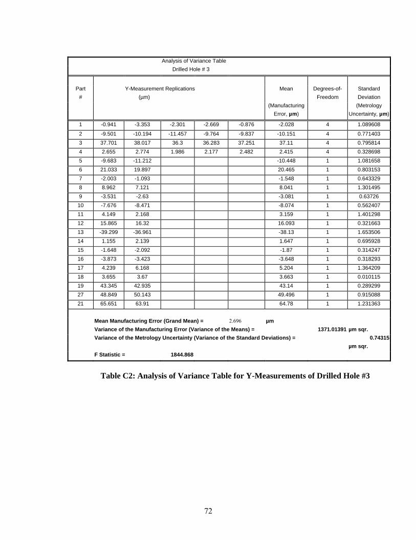
Analysis of Variance Table Drilled Hole # 3

Part Y-Measurement Replications Mean Degrees-of- Standard

# (µm) Freedom Deviation (Manufacturing (Metrology Error, µm) Uncertainty, µm)

1 -0.941 -3.353 -2.301 -2.669 -0.876 -2.028 4 1.089608

2 -9.501 -10.194 -11.457 -9.764 -9.837 -10.151 4 0.771403 3 37.701 38.017 36.3 36.283 37.251 37.11 4 0.795814 4 2.655 2.774 1.986 2.177 2.482 2.415 4 0.328698 5 -9.683 -11.212 -10.448 1 1.081658 6 21.033 19.897 20.465 1 0.803153 7 -2.003 -1.093 -1.548 1 0.643329 8 8.962 7.121 8.041 1 1.301495 9 -3.531 -2.63 -3.081 1 0.63726

10 -7.676 -8.471 -8.074 1 0.562407 11 4.149 2.168 3.159 1 1.401298 12 15.865 16.32 16.093 1 0.321663 13 -39.299 -36.961 -38.13 1 1.653506 14 1.155 2.139 1.647 1 0.695928 15 -1.648 -2.092 -1.87 1 0.314247 16 -3.873 -3.423 -3.648 1 0.318293 17 4.239 6.168 5.204 1 1.364209 18 3.655 3.67 3.663 1 0.010115 19 43.345 42.935 43.14 1 0.289299 27 48.849 50.143 49.496 1 0.915088 21 65.651 63.91 64.78 1 1.231363

Mean Manufacturing Error (Grand Mean) = 2.696 µm Variance of the Manufacturing Error (Variance of the Means) = 1371.01391 µm sqr. Variance of the Metrology Uncertainty (Variance of the Standard Deviations) = 0.74315 µm sqr. F Statistic = 1844.868

Table C2: Analysis of Variance Table for Y-Measurements of Drilled Hole #3

72

Analysis of Variance Table Milled Hole # 3

Part X-Measurement Replications Mean Degrees-of- Standard

# (µm) Freedom Deviation (Manufacturing (Metrology Error, µm) Uncertainty, µm)

1 10.925 12.514 14.288 14.256 11.326 12.662 4 1.581885

2 13.556 12.913 11.694 12.823 11.41 12.479 4 0.89792 3 11.841 14.149 15.154 14.161 14.668 13.994 4 1.273478 4 10.459 9.008 8.763 7.597 8.788 8.923 4 1.020844 5 15.985 15.51 15.747 1 0.335826 6 11.404 12.2 11.802 1 0.563083 7 5.749 5.278 5.513 1 0.333129 8 -14.611 -14.951 -14.781 1 0.24007 9 11.294 10.412 10.853 1 0.623767

10 10.541 10.89 10.715 1 0.246816 11 11.078 13.796 12.437 1 1.921895 12 8.509 12.653 10.581 1 2.930723 13 20.172 18.027 19.1 1 1.51661 14 13.281 13.848 13.565 1 0.401234 15 14.088 12.43 13.259 1 1.172022 16 10.036 11.259 10.648 1 0.864516 17 12.031 14.395 13.213 1 1.671714 18 10.742 10.573 10.658 1 0.11936 19 15.688 14.681 15.184 1 0.712113 27 13.666 12.669 13.167 1 0.705367 21 11.56 11.072 11.316 1 0.345266

Mean Manufacturing Error (Grand Mean) = 11.227 µm Variance of the Manufacturing Error (Variance of the Means) = 86.919903 µmsqr. Variance of the Metrology Uncertainty (Variance of the Standard Deviation) = 1.385941 µmsqr. F Statistic = 62.71543

Table C3: Analysis of Variance Table for X-Measurements of Milled Hole #3

73

Analysis of Variance Table Milled Hole # 3

Part Y-Measurement Replications Mean Degrees-of- Standard

# (µm) Freedom Deviation (Manufacturing (Metrology Error, µm) Uncertainty, µm)

1 10.974 11.803 11.292 12.208 11.489 11.553 4 0.473984

2 10.464 10.304 11.124 10.35 9.867 10.422 4 0.453149 3 11.358 10.515 10.819 11.335 11.759 11.157 4 0.489981 4 11.982 11.381 11.349 11.707 11.567 11.597 4 0.259562 5 6.149 6.483 6.316 1 0.236022 6 11.189 11.07 11.129 1 0.083622 7 11.958 11.473 11.715 1 0.343244 8 -13.513 -12.861 -13.187 1 0.460581 9 12.036 11.498 11.767 1 0.381003

10 13.702 14.645 14.174 1 0.666257 11 16.416 15.868 16.142 1 0.387077 12 12.733 12.709 12.721 1 0.017536 13 18.048 19.018 18.533 1 0.685809 14 14.497 14.514 14.505 1 0.012141 15 12.851 11.301 12.076 1 1.095818 16 11.425 12.569 11.997 1 0.80922 17 10.257 12.566 11.411 1 1.632596 18 12.564 11.773 12.168 1 0.559039 19 11.751 12.123 11.937 1 0.263001 27 11.97 12.856 12.413 1 0.626468 21 13.651 13.42 13.535 1 0.163193

Mean Manufacturing Error (Grand Mean) = 12.838 µm Variance of the Manufacturing Error (Variance of the Means) = 80.800102 µm sqr. Variance of the Metrology (Variance of the Means) = 0.299211 µm sqr. F Statistic = 270.0435

Table C4: Analysis of Variance Table for Y-Measurements of Milled Hole #3.

74

Analysis of Variance Table Drilled Hole # 9

Part X-Measurement Replications Mean Degrees-of- Standard

# (µm) Freedom Deviation (Manufacturing (Metrology Errors, µm) Uncertainty, µm)

1 7.837 7.521 7.277 8.075 6.667 7.475 4 0.544309

2 4.903 5.352 5.411 4.946 6.571 5.437 4 0.674551 3 21.018 20.875 19.423 22.19 22.438 21.189 4 1.205255 4 3.952 2.542 3.057 1.662 3.372 2.917 4 0.867943 5 7.962 9.512 8.737 1 1.095818 6 4.37 5.79 5.08 1 1.004106 7 3.724 3.736 3.73 1 0.008092 8 -13.96 -14.961 -14.461 1 0.708068 9 3.099 1.667 2.383 1 1.012873

10 -2.782 -3.345 -3.064 1 0.398541 11 2.476 3.744 3.11 1 0.896884 12 -16.38 -15.505 -15.943 1 0.619051 13 -43.098 -41.484 -42.291 1 1.141673 14 4.272 2.942 3.607 1 0.940718 15 7.968 8.286 8.127 1 0.224558 16 3.741 -0.134 1.803 1 2.740556 17 10.651 5.971 8.311 1 3.30903 18 0.651 -0.635 0.008 1 0.909698 19 29.827 30.695 30.261 1 0.613656 27 27.004 26.467 26.736 1 0.37966 21 15.547 16.31 15.928 1 0.53948

Mean Manufacturing Error (Grand Mean) = 4.985 µm Variance of the Manufacturing Error (Variance of the Means) = 511.44179 µm sqr. Variance of the Metrology Uncertainty (Variance of the Standard Deviations) = 1.189403 µm sqr. F Statistic = 429.9987

Table C5: Analysis of Variance Table for X-Measurements of Drilled Hole #9

75

Analysis of Variance Table Drilled Hole # 9

Part Y-Measurement Replications Mean Degrees-of- Standard

# (µm) Freedom Deviation (Manufacturing (M etrology

UnceError, µm) rtainty, µm)

1 -22.324 -21.057 -21.072 -19.226 -20.386 -20.813 4 1.130235

2 7 7 69 6 -30.789 4 0.673669 -31.5 -30.16 -30.8 -31.29 -30.0453 4 1 5 9 4 0.817194 11.15 10.97 12.37 10.55 10.239 11.06 4 6 3 34 8 -17.819 4 0.901909 -16.26 -18.17 -18.2 -17.86 -18.5555 5 4 -25.169 1 0.658168 -25.63 -24.70 6 9 4 -12.032 1 0.010783 -12.03 -12.02 7 7 7 1 0.820011 -14.55 -15.71 -15.137 8 5 7 -20.844 1 1.122115 -20.0 -21.63 9 2 1 0.388426 -8.07 -8.621 -8.347

10 4 4 -22.339 1 0.388428 -22.61 -22.06 11 9 3 -20.004 1 0.388428 -20.27 -19.7 12 4 1 -27.557 1 0.107897 -27.63 -27.48 13 6 2 1 0.873956 -60.48 -61.72 -61.104 14 5 4 1 0.345266 -14.46 -14.95 -14.709 15 2 7 1 1.650811 -22.20 -19.86 -21.034 16 8 6 1 0.55027 -20.50 -21.28 -20.897 17 9 3 -23.346 1 1.532124 -24.42 -22.26 18 2 2 -24.757 1 0.204997 -24.61 -24.90 19 6 6 24.086 1 0.226585 23.92 24.24 27 5 5 27.145 1 0.410002 26.85 27.43 21 2 8 1 0.399218 45.53 44.96 45.25

Mean Manufacturing Errp Grand Mean) = 2.696 µm r ( Variance of the Manufacturing Error (Variance of the Means) 1924.78242 µm sqr. = Variance of the Metrology Uncertainty (Variance of the Standard Deviations) = 0.677527 µm sqr. F Statistic = 2840.895

Table C6: Analysis of Variance Table for Y-Measurements of Drilled Hole #9.

76

Analysis of Variance Table 9 Milled Hole #

Part X-Measurement Replications Mean Degrees-of- Standard

# (µm) Freedom Deviation (Manufacturing (Metrology Error, µm) Uncertainty, µm)

1 16.844 17.036 15.541 14.392 17.315 16.226 4 1.230574

2 12.421 11.37 11.843 10.819 11.881 11.667 4 0.60236 3 13.545 13.164 14.556 12.291 12.893 13.29 4 0.842547 4 16.253 14.369 17.07 17.63 17.078 16.48 4 1.278243 5 20.363 21.506 20.935 1 0.808548 6 20.476 19.172 19.824 1 0.922513 7 5.013 6.687 5.85 1 1.184158 8 -9.427 -10.124 -9.776 1 0.492952 9 16.628 17.302 16.965 1 0.476088

10 9.825 9.42 9.623 1 0.285924 11 13.21 15.644 14.427 1 1.720935 12 -1.594 -0.473 -1.033 1 0.792361 13 25.29 26.453 25.871 1 0.822705 14 23.735 23.692 23.714 1 0.030349 15 21.171 22.602 21.886 1 1.012195 16 6.42 6.26 6.34 1 0.113291 17 19.974 19.786 19.88 1 0.132844 18 17.862 16.369 17.116 1 1.056029 19 25.863 25.488 25.675 1 0.265017 27 20.897 19.802 20.349 1 0.774155 21 17.456 17.815 17.635 1 0.253561

Mean Manufacturing Error (Grand Mean) 14.794 µm Variance of the Manufacturing Error (Variance of the Means) = 158.373624 µm sqr. Variance of the Metrology Uncertainty (Variance of the Standard Deviations) = 0.833741 µm sqr. F Statistic = 189.9553

Table C7: Analysis of Variance Table for X-Measurements of Milled Hole #9.

77

Part #

1

2 3 4 5 6 7 8 9

10 11 12 13 14 15 16 17 18 19 27 21

Analysis of Variance Table Milled Hole # 9

Y-Measurement Replications Mean Degrees-of- Standard (Micrometers) Freedom Deviation

(manufacturing (Metrology Error) Uncertainty)

7.141 6.897 7.538 7.477 7.736 7.358 4 0.335069

10.406 10.59 10.773 10.62 10.559 10.59 4 0.131265 5.493 5.768 4.791 5.249 5.005 5.261 4 0.386382 5.997 5.905 6.027 6.058 5.783 5.954 4 0.111295 3.815 5.219 4.517 1 0.992643

31.799 31.219 31.509 1 0.410009 6.012 5.325 5.669 1 0.485532 -17.7 -18.738 -18.219 1 0.733687 8.392 8.667 8.53 1 0.194213

10.101 9.567 9.834 1 0.377637 10.559 10.681 10.62 1 0.086317 20.325 20.081 20.203 1 0.172633 17.807 17.67 17.738 1 0.097107 10.452 9.583 10.017 1 0.615006 11.505 10.101 10.803 1 0.992644 6.744 6.561 6.653 1 0.129475 7.355 8.057 7.706 1 0.496322 3.754 3.937 3.845 1 0.129475 6.668 7.523 7.095 1 0.604217 9.964 10.91 10.437 1 0.668952 38.91 38.086 38.498 1 0.582635

Mean Manufacturing Error (Grand Mean) = 12.838 micrometers Variance of the Manufacturing Error (Variance of the Means) = 274.906987 micrometer sqr. Variance of the Metrology Uncertainty (Variance of the Standard Deviations) = 0.185294 micrometer sqr. F Statistic = 1483.63

Table C8: Analysis of Variance Table for Y-Measurements of Milled Hole #9.

78

ariance Table Analysis of V ole # 15 Drilled H

Part X-Measurement Replications an Degrees- d Me of- Standar

# icrom edom ion (M eters) Fre Deviat (Manufacturing y (Metrolog

) nty) Error Uncertai

1 54 41 7 36 33 67 4 77 -6.4 -5.3 -6.4 -6.8 -7.2 -6.4 0.7055

2 902 15 22 4 49 -11. -12.1 -11.948 -12.573 -12.07 -12.1 0.26703 91 44 4.542 4.221 14.74 87 4 58 14.1 15.2 1 1 14.5 0.43224 79 26 3.448 1.862 1.556 34 4 76 -3.4 -3.3 - - - -2.7 0.94395 6 82 4 1 34 2.10 3.0 2.59 0.69056 98 58 77 1 61 -3.9 0.4 -1. 3.15057 1 49 8 1 59 -5.3 -5.2 -5.2 0.04318 523 455 989 1 68 -20. -19. -19. 0.75529 89 67 28 1 17 -2.2 -2.1 -2.2 0.0863

10 .19 .945 068 1 4 -16 -15 -16. 0.172611 33 22 26 1 55 -3.4 -3. -3.3 0.151012 05 46 26 1 56 -12.4 -13.0 -12.7 0.453113 016 .862 939 1 45 -54. -55 -54. 1.305514 13 13 13 1 72 -7.8 -9.6 -8.7 1.273115 .727 44 185 1 62 -10 -9.6 -10. 0.766016 27 15 21 1 19 -9.8 -9.4 -9.6 0.291317 99 11 55 1 05 -6.6 -8.0 -7.3 0.927918 14 45 8 1 07 -2.9 -2.0 -2.4 0.615019 19.82 20.325 20.073 1 0.356057 1 27 83 1 0.151059 23.59 23.376 23.421 3.288 2.96 3.616 1 0.463953

Mean Manufacturing Error (Grand Mean) = -4.521 micrometers Variance of the Manufactu Variance of the Means) = 565.99933 micrometer sqr. ring Error ( Variance of the Metrology Error (Variance of the Standard Deviations) = 0.710005 micrometer sqr. F Statistic = 797.1762

Table C9: Analysis of Variance Table for X-Measurements of Drilled Hole #15.

79

Analysis of Variance Table Drilled Hole # 15

Part Y-Measurement Replications Mean Degrees-of- Standard

# (Micrometers) Freedom Deviation (Manufacturing (Metrology

Error) Uncertainty)

1 -30.075 -29.633 -28.046 -27.893 -28.793 -28.888 4 0.958113

2 -29.053 -29.404 -29.099 -29.022 -29.221 -29.16 4 0.155985 3 25.436 25.787 21.469 26.031 24.796 24.704 4 1.867158 4 -31.54 -31.403 -31.769 -31.174 -31.418 -31.461 4 0.217243 5 -29.968 -29.343 -29.655 1 0.442373 6 -20.737 -21.133 -20.935 1 0.28053 7 -25.879 -25.055 -25.467 1 0.582642 8 -19.318 -19.867 -19.592 1 0.388421 9 -27.069 -27.847 -27.458 1 0.55027

10 -25.62 -25.803 -25.711 1 0.129471 11 -23.239 -23.651 -23.445 1 0.291314 12 -6.256 -7.462 -6.859 1 0.852378 13 -63.965 -61.783 -62.874 1 1.542907 14 -18.021 -18.478 -18.25 1 0.323685 15 -20.981 -22.766 -21.873 1 1.262384 16 -22.064 -21.805 -21.935 1 0.183423 17 -28.229 -28.076 -28.152 1 0.107897 18 -30.289 -26.321 -28.305 1 2.805298 19 22.583 23.163 22.873 1 0.410002 27 31.479 32.15 31.815 1 0.474744 21 23.407 24.048 23.727 1 0.453164

Mean Manufacturing Error (Grand Mean) = 2.696 micrometers Variance of the Manufacturing Error (Variance of the Means) = 2410.274 micrometer sqr. Variance of the Metrology Uncertainty (Variance of the Standard Deviations) = 0.981564 micrometer sqr. F Statistic = 2455.544

Table C10: Analysis of Variance Table for Y-Measurements of Drilled Hole #15.

80

Analysis of Variance Table Milled Hole # 15

Part f- Standard X-Measurement Replications Mean Degrees-o

# Deviation (Micrometers) Freedom y (Manufacturing (Metrolog

Error) Uncertainty)

1 6.775 7.523 8.041 8.575 7.568 4 0.75504 6.927

2 -3.799 -4.959 -3.51 -2.777 8 -3.461 4 1.033854 -2.253 5.737 6.497 4 0.976229 5.371 7.416 7.553 6.409 4 13.245 12.405 12.082 4 1.392083 11.719 9.857 13.184 5 12.36 10.254 11.307 1 1.488962 6 7.477 10.925 9.201 1 8446 2.437 -0.534 -1.404 -0.969 1 0.615007 8 -31.204 -27.39 -29.297 1 2.697393 9 6.104 5.188 5.646 1 0.647376

10 -2.747 -3.357 -3.052 1 0.431584 11 6.485 5.821 1 0.938694 5.157 12 -8.911 -7.706 -8.308 1 0.852378 13 5.188 6.5 1 0.927905 5.844 14 9.964 9.521 43 1 0.312898 9.715 13.519 15.442 14.481 1 1.359483 16 0.26974 0.198 0.58 0.389 1 17 4.704263 8.362 1.709 5.035 1 18 2.35 2.426 2.388 1 0.053947 19 9.628 8.759 9.193 1 0.615007 27 8.118 6.287 7.202 1 1.294751 21 -3.769 -3.174 -3.471 1 0.420794

Mean Manufacturing Error (Grand Mean) = 3.625 micrometers Variance of the Manufacturing Error (Variance of the Means) = 202.311028 micrometer sqr. Variance of the Metrology Uncertainty (Variance of the Standard Deviations) = 1.921037 micrometer sqr. F Statistic = 105.3134

Table C11: Analysis of Variance Table for X-Measurements of Milled Hole #15.

81

82

Analysis of Variance Table Milled Hole # 15

Part Y-Measurement Replications Mean Degrees-of- Standard

# (Micrometers) Freedom Deviation (Manufacturing (Metrology

Error) Uncertainty)

1 3.418 3.784 3.271 4 0.451696 2.579 3.448 3.128

2 3.555 3.448 3.525 4 0.161484 3.296 3.601 3.723 3 448 3.845 3.784 3.668 4 0.265521 3.326 3.937 3.4 4 0.417099 2.319 2.197 2.06 1.74 1.282 1.92 5 0.473 1 0.453163 0.153 0.793 6 21.576 22.064 1 0.690532 22.552 7 -0.702 0.29 1 1.402647 1.282 8 -24.048 -24.338 1 0.410009 -24.628 9 -0.153 0.412 1 0.79843 0.977

10 3.723 1 0.345267 3.967 3.479 11 3.334 1 0.917115 3.983 2.686 12 22.141 1 0.107897 22.064 22.217 13 12.764 1 1.758702 11.52 14.008 14 5.608 1 0.183423 5.478 5.737 15 2.457 1 0.53948 2.838 2.075 16 -0.854 1 0.086317 -0.793 -0.916 17 -1.114 1 0.539479 -1.495 -0.732 18 2.586 1 0.226582 2.426 2.747 19 7.523 7.042 1 0.679745 6.561 27 1 0.226582 7.904 7.584 7.744 21 30.777 1 0.496318 31.128 30.426

Mean Manufacturing Error (Grand Mean) = 12.838 micrometers Variance of the Manufacturing Error (Variance of the Means) = 417.453169 micrometer sqr. Variance of the Metrology Uncertainty (Variance of the Standard Deviations) = 0.328871 micrometer sqr. F Statistic = 1269.352

sis of Variance Table for Y-Measurements of Milled Hole #15.

Table C12: Analy

82

APPENDIX D: Derivation of the Variance of Length Equation

ive the formula (35). From equation (33), the quantity In this appendix we der L is

tion of the four error terms . implicitly a func ),(),,(),,(),,( 22112211 yxEyxEyxEyxE yyxx

L can be expanded as a Taylor series around (0, 0, 0, 0) to the first order as

,(),,(),,(( 12211 xEyxEyxEL yxx

),(),()0,0,0,0(

),(),()0,0,0,0(

),(),()0,0,0,0(

),(),()0,0,0,0(

)0,0,0,0()),(),

2222

1111

2222

1111

221

yxEyxE

L

yxEyxE

L

yxEyxE

L

yxEyxE

LLyxEy

yy

yy

xx

xx

y

∂∂

+

∂∂

+

∂∂

+

∂∂

+

=

(D1)

of (33) By implicit differentiation

,(),,(),,(),,(( 22112211 yxEyxEyxEyxEL yyxx

)),(),((

)),(),,(),,(),,((),(

))

222111 xx

2211221111

yxExyxEx

yxEyxEyxEyxEyxE

Lyyxx

x

−−+=∂

∂ (D2)

ions (33) and (34), it is clear that

).0,0,0,0(0 LL = At (0, 0, 0, Note that, comparing equat0) equation (D2) becomes

)(),()0,0,0,0(

2111

0 xxyxE

LLx

−=∂∂ (D3)

By repeating this argument for each of the four error terms and dividing by

0L ,

0

21

22

0

21

11

0

21

22

0

21

11

)(),(

)(),(

)(),(

)(),(

Lyy

yxEL

Lyy

yxEL

Lxx

yxEL

Lxx

yxEL

y

y

x

x

−−=

∂∂

−=

∂∂

−−=

∂∂

−=

∂∂

(D4)

83

Introducing (D4) into (D1) one gets

),()(

),()(

),()(),()(

220

2111

0

21

20

2111

0

210

yxEL

yyyxE

Lyy

yxEL

xxyxEL

xxLL

yy

xx

−−

−+

2−

−−

+= (D5)

Now, one can apply the sum of variance formula, using the fact that the variance of a constant is zero in order to get equation (35).

84

APPENDIX E: MACSYMA Program to Generate the Kinematic Model Error

y,dzy]$

:[eyz,dxz,axz,exz,dyz,ayz,dzz]$ st:append(list1,list2,list3)$

o a ong */ 0]$

w2:[0,1,0,y]$ row3:[0,0,1,0]$ row4:[0,0,0,1]$

long y */ w1:[1,-ezy,eyy,dxy-axy*y]$

row2:[ezy,1,-exy,dyy]$ w3:[-eyy,exy,1,dzy]$

rrrty:matrix(row1,row2,row3,row4)$ /* Final y motion relative to referenc e

y:rty.errrty$ nstruct the homogeneous transformation of x relative to y */

Ideal motion along x */ row1:[1,0,0,x]$ row2:[0,1,0,0]$ row3:[0,0,1,0]$ row4:[0,0,0,1]$ ytx:matrix(row1,row2,row3,row4)$ /* Rotational and translational errors along x */

w1:[1,-ezx,eyx,dxx]$

exx,1,dzx]$ w4:[0,0,0,1]$

errytx:matrix(row1,row2,row3,row4)$ Final error matrix of x rlative to y motion */

w2:[0,1,0,-y]$ row3:[0,0,1,z]$ row4:[0,0,0,1]$ tw:matrix(row1,row2,row3,row4)$

Equations /* Construct the list of error components */ list1:[ezy,eyy,dxy,axy,exy,dy

st2:[ezx,eyx,dxx,exx,dyx,dzx,ezz]$ lilist3li/* Construct the homogeneous transformation of y relative to reference */ /* Ideal moti n l y

w1:[1,0,0,roro

rty:matrix(row1,row2,row3,row4)$ /* Rotational and translational errors aro

rorow4:[0,0,0,1]$ e

e coordinat s */ rt/* Co/*

rorow2:[ezx,1,-exx,dyx]$ row3:[-eyx,ro

/*ytx:ytx.errytx$ /* Construct the relative position of the workpiece relative to x */ row1:[1,0,0,-x]$ ro

x

85

/* N rotational and tran ational e or here */ o sl rr Final error matrix of workpiece relative to the reference */

rtw:rty.ytx.xtw$ /* Construct the motion of z relative to the reference system

otion of z */ 1:

w3:[0,0,1,z]$ row4:[0,0,0,1]$ rtz:matrix(row1,row2,row3,row4)$

otational and translational errors of z */ zz,eyz,dxz-axz*z]$

,-exz,dyz-ayz*z]$ w3:[-eyz,exz,1,dzz]$ w4:[0,0,0,1]$

/ z:rtz.errrtz$

lative to z */ tt:ident(4)$ Final error matrix of tool relative to z */

Get the inverse of rtt */ $

y:taylor(err[2,4],list,0,1); ez:taylor(err[3,4],list,0,1);

/*

*/ /* Ideal mrow [1,0,0,0]$ row2:[0,1,0,0]$ ro

/* Rrow1:[1,-eow2:[ezz,1r

roroerrrtz:matrix(row1,row2,row3,row4)$ /* Final error matrix of z relative to reference *rt/* Tool rez/*rtt:rtz.ztt$ /*rttinv:rtt^^-1/* Compute the final error matrix */ err:rttinv.rtw$ /* Linearize the displacement error terms by a first order Taylor Series about 0 */ ex:taylor(err[1,4],list,0,1); e

86

APPENDIX F: Circle Fit Algorithm

ore we describe the algorithm for computing the least squares fitting of a circle we d to introduce the notion of a symmetric positive definite (SPD) matrix. A real

Befee nn× n

is symmetric if it equals its tra spon se, i.e. matrix A TAA = . It is positive definite if T for all n-vectors x. There are some useful properties of a SPD matrix. First of

value falls on the main diagonal, all of whose entries are ositive. Furthermore, if the matrix is symmetric and the main diagonal is positive and

the main diagonal entry of each row is larger tha the f the absolute values of all e other elements of that row then the matrix is SPD eans that if we add a large

p l symmetric matrix, then we k below. Finally a SPD matrix

0>Axxall the largest entry in absolutep

n sum o. This mth

enough ositive multiple of the identity matrix to the originaan ma e it SPD. This property plays a part in the algorithmc

A can be factored as

RRLLA TT == (F1) where L is a lower triangular matrix and R is an upper triangular matrix. Either of these factorizations is called a Cholesky factorization. In terms of L a matrix equation of the orm f

bxLLAx T == (F2)

can be solved in two steps by

vxLbLv

T =

= (F3)

here v is an intermediate vector. The algorithm for computing L is relatively simple and

hwcan also be used to detect when A is not SPD. This check is used in t e circle fitting program. The Cholesky algorithm begins by setting

1111L = A (F4)

hen going down the first column

T

11

1Ai=1

2

LL

ntoifor

i

= (F5)

For column j = 2 to n

87

jjL

j

ij

j

k

L

n−

−

=

=

1

1

1

(F6)

The c ty under e square root sign is positive. If not then the main circle fitting algorithm is signaled

atrix t ositive definite. For further discussion of the Cholesky ct ion see Nash [30].

he e fittin ethod and that of Marquardt L erg. F ing criteria see Dennis nd Schnabel [33]. Start with a set of points in the plane . Then

define

i −−+−= (F7) where notation let

jkjjjj LAL ∑−= 2

tojifor += 1

kjkikij LLA ∑

=

−1

test on the positive definiteness of A is done by che king whether a quanti

ththat the m A is no p

orizatfa T–

circl g algorithm is a combination of Newton’s Mevenb or the basic algorithm see Nash [30] and for stopp

a ),(,),,( 11 NN yxyxthe residual functions

222 )()(),,( rbyaxrbaR ii

(a, b) is the center and r is the radius to be determined. In order to simplify .,, rpbpa === Let Tpppp ),,(=321p 321 . Form the sum-of-squares

n functio

)()( ( )∑=

=N

ii pRpS

1

2 (F8)

The object is to minimize S over a, b, and r. At its minimum any constant multiple of the gradient of S is zero. For notation, let

)(21)( pSpg ∇= (F9)

The components of are given by

)( pg

[ ][ ]

[ ][ ]

[ ][ ]∑ ∑

∑ ∑

∑∑

= =

= =

==

−−−+−=∂∂

=

−−−−+−=∂∂

=

−−−−+−=∂∂

=

N

i

N

iii

ii

N

i

N

iiii

ii

N

iiii

N

i

ii

pppypxppR

pRpg

pyppypxppR

pRpg

pxppypxppR

pRpg

1 13

23

22

21

33

1 12

23

22

21

22

11

23

22

21

1 11

2)()()()()(

)(2)()()()()(

)(2)()()()()(

(F10)

Let

88

⎟⎟⎟⎟⎟⎟⎞∂∂ 11 RR

⎠⎜⎜⎜⎜⎜⎜⎛

∂∂∂

∂∂∂∂

=321

1

pR

pppR

JNN

R is the colu vect th co ents en fro 10) re en oluector g is

T

⎝ ∂ 1p ∂ 32 p∂RRN

(F11)

iR , th m (F the th e elem t c mn If mn or wi mpon

v

RJg = (F12)

he next job is to estim e ste gth that ill take the point

ate th p len w pT to a new point in such a way that pdp + 0)( =pd+p

rite g . This can be done by using the Taylor series to

w

)2()()3

1Opdpgg ki +

∂)( p( pdp

pk

gi

ki

∂+= ∑

=

+ (F13)

r In order to select

pd so fo .3,,1=i that 0)( =+ pdpg one needs to solve

),,()( pi3

d∑1k

rbgg

p ik −=∂∂

apk=

(F14)

r w, fr 10) fo 3,,1=i . No om (F

∑⎢⎢∂

=p= ⎦

⎤

⎣ ∂∂∂

i jk

i

j

i

k

i

k

ppp

Rp

pR

pR

1

2

)()()(

ote that

⎥⎥

⎡∂N

+ i pR )(∂∂

∂p

p)(

∂ jg(F15)

N

⎪⎪⎩

⎪⎪⎨

⎧

==−====≠

=∂∂

∂

322212

0

)(2

jkjkjk

jk

ppp

R

jk

i (F16)

so that (F15) can be written in matrix form as

(F17)

JJH T=

89

N

ow (F14) can be written, using (F12), as

RJgpHd T−=−= (F18)

lthough H is symmetric it is not ne ily po ay be ngular. The s ing of (F18) ma nt. This is discussed by Marquardt 963]. Also, se Nash [ stead of (F19) consider

JT

A cessar

y also need sitive def

adjustmeinite and in fact m

si c la[1 e ]. In

(J ) pdI RTJ−=+

we scale the rameters by a matrix with only a positive main diagonal then we can rite

)ˆ( 1 RpRp

Dp

==

=−

(F20)

hen, in terms of the scaled parame (F19) co ld be wri en

J TT ˆˆˆˆ −=+

λ (F19) If paw

)()ˆ(DR̂

p̂

p T ters, u tt

( ) ˆ RJpdIJ λ (F21)

here, it is not hard to s

pJ

w how that

pDdpd

DpJ

=

−

ˆ)(ˆ(ˆ 1

(F22)

hen, (F21) bec mes

=)

T o

( )( ) ( ) RJD−=pDdIDD TT11− +JJ T1 T− −λ (

r

F23) o

( ) RJpdDJJ TT −=+ λ (F24)

In Nash [30], D is selected as

( ) φ+= iiT

ii JJD (F25) where φ is set chosen so that the scale is not too small. Before describing the algorithm we to select stopping criteria for the final algorithm. For this we choose criteria suggested by Dennis and Schnabel [33]. These criteria depend on the fact that near the optimum both the gradient and the difference between succeeding parameter vectors should be near zero. The relative gradient will be used instead of

90

simply the gradient since it is insensitive to scaling and for the parameters the relative hange in t e parame rs will b . The iteric h te e used se cr a are

( )

32

)1(

)1()(

31

31

1

2 1, ⎟⎞i

31

)(max

maxma

ε

ε

≤−

≤⎜⎝

⎛

−≤≤

=

≤≤

∑

ki

ki

k

i

N

k

i

pp

R

p

where the mpone f the g t

1,max

max

1,x i

⎠−

ip

ig

(F26)

co nts o radien g are computed in (F12) and ε is t ach e epsilon wh is tha hine n er that w en added o 1 return 1. The algori can b ted as 1. Initiali

0.0105.00001.0

pp

iter

rba

=

=

⎟⎟⎟

⎠

⎞

⎜⎜⎜

⎝

⎛

(27)

2. While perform the following operations

2.1 If loop_count > 0 set

he m inich t mac umb h t s

thm e sta follows. ze

0

0

0

0

0p =

0_ countloop =20=max_

4decinc ==φ=λ

itercountloop max__ <dec*λλ =

2.2

2.3

2.4 Form the Jacobian matrix J using (F11)

∑=

=N

iiRf

1

2

( ) ( )

( ) ( ) ⎟⎟⎟⎟

⎠

⎞

⎜⎜⎜⎜

⎝

⎛

−−+−

−−+−=

23

22

21

23

221

211

ppypx

ppypxR

NN

91

92

2.5 Form the gradient vector g using (F12). This test uses f.

2.6 Perform the gradient test in (F26)

2.7 If the test is true exit with the final parameters p , otherwise continue

2.8 If loop_count > 0 then perform the relative parameter test

2.9 If that test is true exit with the final parameters p , otherwise continue

2.10 Form JJH T=

2.11 Set flag = -1 and augment_count = 0

2.12 While flag < 0 perform the following operations

2.12.1 Set augment_count = augment_count + 1 2.12.2 If augment_count > 1 then set inc*λλ = 2.12.3 Set )(HdiagD = 2.12.4 Using (F24) and (F25) form DHaugH λ+= 2.12.5 Perform the Cholesky decomposition as given in (F4) to (F6) and return L

and flag, where flag = -1 if not positive definite and +1 if it is. 2.12.6 Continue the while loop. For sufficiently large λ the augmented matrix

will become positive definite. When it does exit the loop and continue. 2.13 Solve RJpdaugH T−=)( for pd using (F3)

2.14 Set ⎪⎩

⎪⎨

⎧

+=+=

=

1__ countloopcountlooppdpp

pp

old

old

2.15 Return to step 2, the beginning of the while loop.

93

APPENDIX G: Analysis of Variance for Computed Orthogonalities from CMM Measurements

Orthogonality Uncertainty Table

Part Measurement Replications (arc sec) Mean df Stand. Dev.

1 2.165 4.387 4.935 9.156 2.116 4.552 4 2.872672 2 11.583 8.341 7.122 10.142 3.885 8.215 4 2.958529

3 2.803 8.321 1.93 7.987 6.22 5.452 4 2.943944 4 -5.523 -5.859 -8.61 -8.631 -8.007 -7.326 4 1.518122 5 -5.834 -3.276 -4.555 1 1.809033

6 -1.076 0.976 -0.05 1 1.450953 7 -0.178 -5.235 -2.707 1 3.576137 8 -12.286 -2.569 -7.427 1 6.870819

9 -5.311 -9.561 -7.436 1 3.004845 10 8.835 11.289 10.062 1 1.735044 11 10.31 10.295 10.303 1 0.010287

12 25.389 25.348 25.368 1 0.028781 13 -8.481 -12.965 -10.723 1 3.171258 14 -14.406 -12.813 -13.609 1 1.126567

15 -3.403 -14.142 -8.772 1 7.593938 16 14.823 12.433 13.628 1 1.690476 17 -7.164 -5.542 -6.353 1 1.146354

18 -6.462 -0.771 -3.617 1 4.024526 19 -13.728 -14.365 -14.047 1 0.450572 27 -9.597 -8.828 -9.213 1 0.543542

21 -6.243 -1.735 -3.989 1 3.188012

Grand Mean = -1.059 Var.of the Means = 80.284741 Unc. Of the Means = 8.960175277Var. of the Stand. Dev. = 8.768066 Unc. Of the Std.

Dev. = 2.961092028

Table G1: Orthogonality Uncertainty Table for Parts Manufactured on the Hurco

Machining Center.

APPENDIX H: Analysis of Variance Tables for Circularities Computed from CMM Measurements

GranVarVar

Inner Circle Circularity Uncertainty Table

Part Measurement Replications (micromet.) Mean df Stand. Dev.

1 18.62 20.25 22.92 21.92 18.11 20.364 4 2.066962 2 19.81 21.39 20.13 18.04 19.25 19.724 4 1.225594

3 19.58 19.35 19.05 20.41 19.64 19.606 4 0.505698 4 20.56 20.58 18.34 17.78 19.5 19.352 4 1.273232 5 30.77 27.03 28.9 1 2.644579

6 22.83 21.47 22.15 1 0.961665 7 25.34 24.16 24.75 1 0.834386 8 21.76 23.03 22.395 1 0.898026

9 17.74 16.46 17.1 1 0.905097 10 18.42 19.3 18.86 1 0.622254 11 22.93 22.12 22.525 1 0.572756

12 22.69 17.59 20.14 1 3.606245 13 19.25 24.58 21.915 1 3.768879 14 16.2 22.7 19.45 1 4.596194

15 22.32 19.49 20.905 1 2.001112 16 20.58 18.23 19.405 1 1.661701 17 17.45 18.87 18.16 1 1.004092

18 22.44 21.71 22.075 1 0.516188 19 18.07 16.44 17.255 1 1.152584 27 16.49 16.65 16.57 1 0.113137

21 27.7 30.53 29.115 1 2.001112

d Mean = 20.986 . of the Means = 7.378079 Uncer. Of the Means 2.716 . of the Stand. Dev. = 3.129735 Uncer. Of the Stand. Dev. 1.769

Table H1: Circularity Results for Inner Slot Surface

94

95

Outer Circle Circularity Uncertainty Table

Part Measurement Replications (micromet.) Mean df Stand. Dev.

1 18.37 17.87 18.02 17.38 19.09 18.146 4 0.63642 2 27.71 28.39 26.09 29.28 29.88 28.27 4 1.474161

3 20.86 19.42 19.2 21.48 21.08 20.408 4 1.029621 4 29.23 22.31 22.57 22.51 23.92 24.108 4 2.933517 5 23.23 24.59 23.91 1 0.961665

6 35.16 36.56 35.86 1 0.989949 7 19.4 16.69 18.045 1 1.916259 8 22.09 22.83 22.46 1 0.523259

9 21.67 23.13 22.4 1 1.032376 10 28.22 24.04 26.13 1 2.955706 11 24.14 22.81 23.475 1 0.940452

12 31.27 32.18 31.725 1 0.643467 13 30.97 32.28 31.625 1 0.92631 14 26.06 22.94 24.5 1 2.206173

15 23.35 26.32 24.835 1 2.100107 16 19.96 22 20.98 1 1.442498 17 25.28 25.86 25.57 1 0.410122

18 23.66 24.11 23.885 1 0.318198 19 24.39 26.08 25.235 1 1.19501 27 27.34 26.55 26.945 1 0.558614

21 46.42 49.32 47.87 1 2.05061

Grand Mean = 26.018 Var. of the Means = 35.83599 Uncer. Of the Means 5.986 Var. of the Stand. Dev. = 2.556287 Uncer. Of the Stand.Dev. 1.599

Table H2: Circularity Results for the Outer Surface