Rochester Institute of Technology Rochester Institute of Technology

RIT Scholar Works RIT Scholar Works

Theses

12-19-2020

A Comparative Study on Statistical and Machine Learning A Comparative Study on Statistical and Machine Learning

Forecasting Methods for an FMCG Company Forecasting Methods for an FMCG Company

Zenah Yaser Alzubaidi zya8366@rit.edu

Follow this and additional works at: https://scholarworks.rit.edu/theses

Recommended Citation Recommended Citation Alzubaidi, Zenah Yaser, "A Comparative Study on Statistical and Machine Learning Forecasting Methods for an FMCG Company" (2020). Thesis. Rochester Institute of Technology. Accessed from

This Master's Project is brought to you for free and open access by RIT Scholar Works. It has been accepted for inclusion in Theses by an authorized administrator of RIT Scholar Works. For more information, please contact ritscholarworks@rit.edu.

RIT

A Comparative Study on Statistical and Machine Learning Forecasting

Methods for an FMCG Company

By

Zenah Yaser Alzubaidi

A Capstone Submitted in Partial Fulfilment of the Requirements for the

Degree of Master of Science in Professional Studies: Data Analytics

Department of Graduate Programs & Research

Rochester Institute of Technology

RIT Dubai

December 19, 2020

RIT

Master of Science in Professional Studies:

Data Analytics

Graduate Capstone Approval

Student Name: Zenah Yaser Alzubaidi

Graduate Capstone Title: A Comparative Study on Statistical and Machine

Learning Forecasting Methods for an FMCG Company

Graduate Capstone Committee:

Name: Dr. Sanjay Modak Date:

Chair of committee

Name: Dr. Ehsan Warriach Date:

Member of committee

Acknowledgments

First and foremost, I would like to thank my thesis advisor Dr. Ehsan Warriach and Head

of Department Dr. Sanjay Modak of the Rochester Institute of Technology for their invaluable

supervision, guidance and support throughout the journey of my capstone project. Their immense

knowledge and plentiful experience in both academic and business perspectives have been key

contributors to this research. Amid these unprecedented times, they have always made themselves

available through the consistent follow-ups and online meetings to ensure I have full clarity and

knowledge of the requirements and steered me in the right direction whenever they thought I

needed it.

I would also like to express my profound gratitude to my parents for providing me with

unfailing support and continuous encouragement throughout the past year of my degree. The

unconditional love, care and prayers they have showered me with were and continue to be the

anchor and light in tough times. My father, who taught me to always improve myself and never

stop learning, and my mother, who always believed in me. This accomplishment would not have

been possible without their support, and therefore I dedicate this research project to them. Thank

you.

Abstract

Demand forecasting has been an area of study among scholars and businessmen ever since

the start of the industrial revolution and has only gained focus in recent years with the

advancements in AI. Accurate forecasts are no longer a luxury, but a necessity to have for effective

decisions made in planning production and marketing. Many aspects of the business depend on

demand, and this is particularly true for the Fast-Moving Consumer Goods industry where the high

volume and demand volatility poses a challenge for planners to generate accurate forecasts as

consumer demand complexity rises. Inaccurate demand forecasts lead to multiple issues such as

high holding costs on excess inventory, shortages on certain SKUs in the market leading to sales

loss and a significant impact on both top line and bottom line for the business. Researchers have

attempted to look at the performance of statistical time series models in comparison to machine

learning methods to evaluate their robustness, computational time and power. In this paper, a

comparative study was conducted using statistical and machine learning techniques to generate an

accurate forecast using shipment data of an FMCG company. Naïve method was used as a

benchmark to evaluate performance of other forecasting techniques, and was compared to

exponential smoothing, ARIMA, KNN, Facebook Prophet and LSTM using past 3 years

shipments. Methodology followed was CRISP-DM from data exploration, pre-processing and

transformation before applying different forecasting algorithms and evaluation. Moreover,

secondary goals behind this paper include understanding associations between SKUs through

market basket analysis, and clustering using KNN based on brand, customer, order quantity and

value to propose a product segmentation strategy. The results of both clustering and forecasting

models are then evaluated to choose the optimal forecasting technique, and a visual representation

of the forecast and exploratory analysis conducted is displayed using R.

Keywords: time series, forecast, machine learning, statistical methods, market basket

analysis

Table of Contents

ACKNOWLEDGMENTS ........................................................................................................................... II

LIST OF FIGURES ..................................................................................................................................... V

LIST OF TABLES .................................................................................................................................... VII

ABSTRACT ................................................................................................................................................ III

CHAPTER 1 ................................................................................................................................................. 1

1.1 BACKGROUND .............................................................................................................................. 1

1.2 PROBLEM STATEMENT ............................................................................................................... 3

1.3 AIMS AND OBJECTIVES .............................................................................................................. 4

1.4 METHODOLOGY ........................................................................................................................... 5

1.5 LIMITATIONS OF THE STUDY .................................................................................................... 7

CHAPTER 2 – LITERATURE REVIEW .................................................................................................... 9

2.1 INTRODUCTION ............................................................................................................................ 9

2.2 TIME SERIES ................................................................................................................................ 10

2.3 STATISTICAL FORECASTING METHODS............................................................................... 12

2.4 MACHINE LEARNING FORECASTING METHODS ................................................................ 15

2.5 CLUSTERING AND PRODUCT CLASSIFICATION ................................................................. 18

CHAPTER 3 – PROJECT DESCRIPTION ................................................................................................ 20

3.1 BUSINESS UNDERSTANDING ................................................................................................... 20

3.2 DATA UNDERSTANDING .......................................................................................................... 23

3.3 DATA PREPARATION ................................................................................................................. 30

3.4 MODELING ................................................................................................................................... 36

3.5 EVALUATION ............................................................................................................................... 49

3.6 DEPLOYMENT ............................................................................................................................. 50

CHAPTER 4 - PROJECT ANALYSIS ...................................................................................................... 51

4.1 DATA EXPLORATION................................................................................................................. 51

4.2 TIME SERIES ANALYSIS ............................................................................................................ 61

4.3 FORECASTING MODELS ............................................................................................................ 66

4.4 CLUSTERING AND MARKET BASKET ANALYSIS ............................................................... 76

4.5 EVALUATION ............................................................................................................................... 81

CHAPTER 5 – CONCLUSION .................................................................................................................. 83

5.1 CONCLUSION ................................................................................................................................... 83

5.2 FUTURE WORK ................................................................................................................................ 84

BIBLIOGRAPHY ....................................................................................................................................... 85

List of Figures

Figure 1: CRISP-DM Methodology .............................................................................................................. 5

Figure 2: Time Series Prediction Process ................................................................................................... 11

Figure 3: Forecasting Performance of ML and Statistical Methods based on sMAPE ............................... 16

Figure 4: Current product segmentation strategy used at FMCG company ................................................ 22

Figure 5: LSTM Cell Architecture .............................................................................................................. 43

Figure 6: Histogram of Net Value ($) ......................................................................................................... 52

Figure 7: Histogram of Delivered Quantity (MSU) .................................................................................... 53

Figure 8: Scatter plot of Delivered Quantity (MSU) vs. Net Value ($) ...................................................... 53

Figure 9: Faceted Scatter plot of Delivered Quantity (MSU) ..................................................................... 54

vs. Net Value ($) by Category .................................................................................................................... 54

Figure 10: Box plot of Delivered Quantity (MSU) by Category ................................................................ 54

Figure 11: Box plot of Delivered Quantity (MSU) by Segment ................................................................. 55

Figure 12: Box plot of Delivered Quantity (MSU) by Category ................................................................ 56

Figure 13: Box plot of Delivered Quantity (MSU) by Segment ................................................................. 56

Figure 14: Box plot of Total Lead Time (days) by Plant ............................................................................ 57

Figure 15: Pie charts of % of orders by Segment ....................................................................................... 58

Figure 16: Pie charts of % of orders by Category ....................................................................................... 58

Figure 17: Pie charts of % of orders by Country ........................................................................................ 58

Figure 18: Pie charts of % of orders by Source .......................................................................................... 58

Figure 19: Stacked Barplot by Category and Replenishment Stream ......................................................... 59

Figure 20: Stacked Barplot by Category and Segment ............................................................................... 59

Figure 21: Stacked Barplot of Total Orders for UAE and Source .............................................................. 60

Figure 22: Stacked Barplot of Total Orders for KW and Source ................................................................ 60

Figure 23: Stacked Barplot of Total Orders for OM and Source ................................................................ 60

Figure 24: Stacked Barplot of Total Orders for BH and Source ................................................................. 60

Figure 25: Stacked Barplot of Total Orders for BH and Source ................................................................. 60

Figure 26: Time Series plot for Actual Shipment Data from July 2018 to July 2020 ................................ 61

Figure 27: Time Series plot for Actual Shipment Data by Month and Year .............................................. 62

Figure 28: Time Series for Actual Shipment Data by Month and Year by Country ................................... 62

Figure 29: Growth of Shipment in Del. MSU by Year ............................................................................... 63

Figure 30: Change rate of Shipment in Del. MSU by Year ........................................................................ 64

Figure 31: Growth of Shipment in Del. MSU by Quarter........................................................................... 65

Figure 32: Change rate of Shipment in Del. MSU by Quarter .................................................................... 65

Figure 33: Growth of Shipment in Del. MSU by Month ............................................................................ 65

Figure 34: Change rate of Shipment in Del. MSU by Month ..................................................................... 66

Figure 35: Naïve Forecast Time Series Output ........................................................................................... 67

Figure 36: SNaïve Forecast Time Series Output ........................................................................................ 67

Figure 37: Exponential Smoothing Forecast Time Series Output .............................................................. 68

Figure 38: Linear Trend Model Time Series Output .................................................................................. 69

Figure 39: Quadratic Trend Model Forecast Time Series Output ............................................................... 69

Figure 40: Time Series Decomposition Plot ............................................................................................... 70

Figure 41: Stationary Plot after first difference is applied .......................................................................... 70

Figure 42: ACF Plot .................................................................................................................................... 71

Figure 43: PACF Plot .................................................................................................................................. 72

Figure 44: Residual Plot for ARIMA(1,1,1)(1,0,0)[6] ................................................................................ 72

Figure 45: ARIMA (30,1,1)X(1,0,1)30 model forecast .............................................................................. 73

Figure 46: Residual Plots for ARIMA (30,1,1)(1,0,1)[30] model .............................................................. 74

Figure 47: Facebook Prophet Forecast........................................................................................................ 74

Figure 48: LSTM Seasonal Forecast ........................................................................................................... 75

Figure 49: KNN Forecast ............................................................................................................................ 76

Figure 50: Total Within Sum of Squares .................................................................................................... 77

Figure 51: Total Between Sum of Squares ................................................................................................. 77

Figure 52: Cluster plot of K=3 .................................................................................................................... 78

Figure 53: Cluster plot of K=8 .................................................................................................................... 78

Figure 54: Top 10 most frequently bought items ........................................................................................ 80

List of Tables

Table 1: Data Dictionary of Shipment Data ................................................................................................ 26

Table 2: Data Dictionary of Segmentation Data ......................................................................................... 27

Table 3: Pros and Cons of Naïve Forecast .................................................................................................. 36

Table 4: Pros and Cons of Linear Trend Model Forecast ........................................................................... 37

Table 5: Pros and Cons of Quadratic Trend Model Forecast ...................................................................... 38

Table 6: Pros and Cons of Exponential Smoothing .................................................................................... 39

Table 7: Pros and Cons of S/ARIMA Model Forecast ............................................................................... 40

Table 8: Pros and Cons of Facebook Prophet ............................................................................................. 42

Table 9: Pros and Cons of LSTM Model .................................................................................................... 43

Table 10: Pros and Cons of KNN Model .................................................................................................... 46

Table 11: Determining AR and MA values for ARIMA model ................................................................. 71

Table 12: Comparison of Evaluation Metrics for the Forecasting Models ................................................. 81

Chapter 1

1.1 Background

The fast-moving consumer goods (FMCG) industry is unlike any other industry in the market where

synchronization between the different nodes within the supply chain plays a critical role towards ensuring

competitiveness and success in the market. Forecasting the demand of finished products is one of the key

elements in the supply planning stage that needs to be given the right attention, as done incorrectly can lead

to a surplus in stock which is cash held in inventory that could be utilized elsewhere, or shortage at the

customer’s end which can adversely impact the profits and customer satisfaction. Having accurate demand

forecasts that closely reflect the reality of the ordering trends and habits of customers will consequently

translate into accurate raw and pack material procurement, production and capacity planning and overall

reduced costs. Traditional forecasting methods have always existed and proved to be sufficient to meet

market requirements in the past. However, the rising competition within FMCGs imposes the need to

combine geographic, demographic, historical, behavioral and microeconomic factors to understand demand

drivers and enable proactive decisions and strategic planning. Managing good relationships between your

distributors, suppliers and customers is a crucial aspect of effectively managing supply chains in any FMCG

company (FMCG). At the heart of these interdependent links is the management of product flow, or more

specifically, management of inventory. Inventory stands as the single biggest asset in the financial balance

sheet of any FMCG, and therefore effectively controlling it will improve productivity, lower operating costs

and working capital as well as improve customer service, which contributes directly to the company’s

bottom line (cash) and top line (profit).

One of the biggest drivers to inefficient stock management is a poor demand forecast. According

to the IBF, for every $1 billion in sales, a 1% over-forecast error can result in losses between $5.5 million

to $7 million annually. Rather than focusing on the “Why”, companies need to look and plan to be one step

ahead at what scenarios are possible, and what they can do to avoid substantial risks and losses ("NEW

REPORT: The Fast-Moving Consumer Goods Forecasting Evolution - Prevedere", 2017). Sales forecasting

is a process that looks at historical data, along with experience and other economic and business factors, to

create best estimates of how the product will likely perform in the future. Any company which sells products

needs to have a forecast of the demand, as it is the key input to many other processes such as production

and capacity planning, raw and pack material procurement, inventory management, advertising and

promotional activities as well as new product launches. Furthermore, all nodes of the supply chain depend

on the accuracy of this data to run their operations; manufacturers need to know how much to produce,

distributors need to know how much to order and stock, and retailers need to know how much to sell.

Inaccuracies in this process often leads to unclarity in supply planning and customer demand levels cannot

be evaluated realistically, leading to order misses and unsatisfied customers. Hence, the performance of a

successful supply chain system concerns mostly with accurate demand information, as this vital data

influences many decisions made.

A synchronized supply chain will source, produce and ship daily what the consumers require and

flow this seamlessly through the network. Over the past 10 years, leading FMCGs in the world which

specialize in a wide range of personal/consumer health, hygiene and care products, have invested heavily

in forecasting techniques and operation research by creating spreadsheet models that optimized forecasts in

more than 90% of the business at each stage of the supply chain (Yang, Li & Zhang, 2012). The work began

with single use forecasting methods such as three-month moving average, which gave insight on short term

planning, however, did not deem fit once product portfolios have developed over the years and market

dynamics and competition have changed the speed at which the businesses must operate to win in the

market. FMCGs are differentiated by the high variety of goods and innovative products that have a short

shelf life, low profit margins and high volumes. Having said that, a one-size-fits-all forecasting technique

is not optimal. Instead of using one method, a mixture of time series, machine learning and other forecasting

methods can be deployed to generate several forecasts and interpreted to generate superior value. Recently,

FMCGs have begun to realize the importance of high visibility across the nodes of the supply chain and the

bullwhip effect of having demand distorted as you go upstream in the supply chain. Moreover, the industry

is known for its volatility and randomness, which poses a challenge in generating accurate forecasts; this is

behind the contribution of many external factors such as trends, seasonality, competitor activities,

promotions, product prices and other economic factors that are difficult to predict. Companies that can

proactively and in real-time meet true market demand are poised to take the lead in their respective markets,

especially in FMCGs where customers have an abundance of product, brand, and retail channel options.

Given the progression of the COVID-19 pandemic throughout the region, forecasts have become

even more volatile to changes within the market. This is particularly true for FMCGs, where sales and

shipments have been severely impacted by border closures and lockdowns, which have made consumers

more cautious and conservative with their purchases. Hence, forecasting consumer demand has become an

even more challenging task for all companies, as it is susceptible to sudden changes in the spread of the

virus and market laws and measures taken, impacting the entire supply chain end to end. This volatility

only highlights the need for adopting accurate forecasting techniques to be able to adjust to real-time market

dynamics, plan raw materials and capacity effectively, and cater to the new purchasing habits of consumers.

Therefore, the comparative study conducted in this paper will not only give perspective on the power of the

different forecasting techniques in serving the needs of the FMCG company, but it will also showcase the

accuracy and performance of the different models in forecasting the next 3-month demand. The

recommended model to deploy will enable the FMCG company on hand to operate with more agility,

transparency, flexibility, and productivity to adapt to the changing production environments and customer

demands, making it more competitive and cost-effective due to efficient and accurate planning.

Moreover, it is known that FMCGs tend to have a wide variety of products that they offer to

customers, which despite the need for it due to competition or other market interventions, can typically add

a level of complexity to the supply chain in terms of planning and material procurement. Therefore, the

clustering techniques deployed in this study categorizes SKUs based on the magnitude of shipment, and

hence their demand, therefore enabling the FMCG to find SKUs that are profitable and fast moving to

further simplify both the product portfolio and supply chain complexity. This will also help to re-focus

efforts on high performing SKUs to further reduce overall supply chain cost in comparison to the existing

segmentation strategy used on their product portfolio.

1.2 Problem Statement

The purpose of this project is twofold: run a comparative study on the performance of statistical

and machine learning time series forecasting models using shipments data from an FMCG to predict the

next 3-month demand of finished products across all categories in Gulf markets, as well as explore product

associations through basket analysis propose a new product segmentation strategy based on the outcome of

clustering. Transactional data of past three-year shipment report acquired from an FMCG company, along

with product segmentation data will serve as inputs to the forecasting and clustering models. The

methodology applied in this study will follow the CRISP-DM, where the data collected will be cleaned,

pre-processed, and transformed before data modeling, evaluation and deployment. Moreover, several time-

series forecasting techniques are explored, starting off with the statistical techniques which are mainly

naïve, Exponential Smoothing, Linear and Quadratic trend models and ARIMA, and comparing the

accuracy of the forecast to machine learning methods such as KNN, LSTM and Facebook Prophet to find

the optimal model. In terms of the clustering analysis, the clustering technique used will be K-means

clustering. The outcome of these models is a demand forecast of the next 3 months using the optimal

forecasting technique derived from the study mentioned above, as well as a re-defined product segmentation

proposal which will aim to improve both bottom line (cash) and top line (profit) margins, as well as help

identify slow-running SKUs to possibly simplify their product portfolio and reduce complexity in the

supply chain.

1.3 Aims and Objectives

Despite gaining increasing attention in the literature with the developments in AI, machine learning

techniques are not yet well established or considered robust enough in terms of their accuracy and

computational requirements as opposed to statistical or traditional methods. The main objective of this

project is to run a thorough and comprehensive study on the performance of statistical and machine learning

time-series forecasting models on predicting the next 3-month demand of SKUs of an FMCG company and

evaluating each one based on their accuracy and performance. This will be accomplished by applying data

analytic techniques such as cleaning, pre-processing, transformation, and then conducting data exploration

to further understand relationships between different attributes and identify key demand drivers. In turn,

decision-making will be faster and effective through structured scenario analysis to analyze the impact of

these key events and causal factors on future sales. It is important to note that the level of granularity is a

top-level 3 month ahead forecast, and not by SKU due to the availability of the data acquired. However,

deploying such predictive analytic methods into the forecasting and clustering process even at a top level

delivers a range of benefits for the FMCG company on hand, which can be split into system, value-added

and strategic benefits:

System Benefits

• Inventory mix improvement by identifying slow-moving SKUs and revising the product portfolio

based on factors of profitability, volatility and volume.

• Better understanding and prediction of customer demand to obtain optimal inventory levels and

reduce probability of shortages/excess at their warehouse, improve cash flow and reduce holding

cost.

• Improving capacity planning at the plant to optimize use of labor and equipment through effective

production scheduling. Forecasting next 3-month demand will help give the company the ability to

effectively plan raw material availability with more agility, transparency and flexibility by adapting

to the changing production environments.

• Optimized transport logistics to meet customer demand by planning on when, how, why and where

the most strategic and cost-effective logistic decisions can be executed.

Value-Added Benefits

• Improving company’s core competency by reducing cash held in inventory, improving service and

increased market share.

• Improved service levels by making sure customers have the right products delivered at the right

time and meeting their requirements through utilizing forecasting methods as a holistic tool to

refine, streamline and enhance the operational, logistical and production cycles. This in turn results

in higher customer satisfaction and increased sales.

• Establish accurate sales quotas for market strategy planners and enable the development of new

products by identifying future demand patterns.

• To direct sales efforts more effectively on promotions and establishing sales of the power-runner

SKUs.

Strategic Benefits

• Greater profitability to the customer’s bottom line.

• Guide top management in overall planning and control of operations and reducing overall costs

associated with unused materials and ensure the right quantity of stocks is always available to fulfill

customer demand.

• Make sound plant expansion decisions.

• Manage finances for the short and long term more effectively and prepare accurate capital budgets.

1.4 Methodology

In order to tackle the problem on hand of finding the optimal forecasting method amongst statistical

and machine learning models, as well as develop a product classification strategy, the CRISP-DM methodology

was followed, as shown in Figure 1.

Figure 1: CRISP-DM Methodology

The process consists of six main steps as outlined below:

1) Business Understanding: First, the project objectives and requirements from a business perspective were

outlined based on discussions with Sales Logistics Leaders within the FMCG company. These objectives

were twofold; to improve on capacity and raw material planning in order to effectively manage inventory

on critical SKUs and predict trends, and second, to propose a new segmentation strategy for SKUs based

on their ordering trends to simplify the product portfolio on slow-moving SKUs which are not profitable

to the business, and only add more complexity to the supply chain. These objectives were used to formulate

clear problem statement ahead of the data mining process, as mentioned above.

2) Data Understanding: The second phase was to collect data and conduct exploratory analysis to better

understand the characteristics and features of the dataset, prior to pre-processing. The data used for the

purpose of this project is one that is acquired by an FMCG company that operates in the Gulf markets and

has products across 4 main categories:

• Fabric & Home Care

• Baby & Feminine Care

• Grooming (Shave & Oral Care)

• Beauty (Skin, Hair and Personal Care

The data collected and used as input to the forecasting and clustering models are:

• Past 18-month shipment report for Gulf Markets at SKU level

• List of Plant/Source Names

• List of Current Segmentation used per SKU

The exploratory analysis was conducted on R Studio and involved several statistical measures to

understand the central tendency of the dataset, missing values and outliers prior to data preparation. This was

done through histograms, scatter plots and box plots to identify noisy data, and relationships between the

different attributes. A time series analysis was also conducted, including time series plots to understand the

trend in shipments with relation to different time periods, as well as understand seasonality, which was critical

before applying any transformation on the dataset.

3) Data Preparation: The next section involves all activities conducted to construct the final dataset to be

used for modeling. This section involved data reduction to simplify the dataset and include only valuable

and relevant columns for the analysis, data smoothing to remove noise data through IQR, as well as

aggregation to combine order quantities for a given day for the time series forecasts, as well as preparing

the dataset for clustering by coding categorical variables and removing unnecessary attributes. Finally,

stationarity and seasonality were addressed by applying transformation methods such as differencing.

4) Modeling: After preparing the dataset, statistical and machine learning time series models were applied

for the first phase of the project, which is forecasting. Methods included were naïve and snaïve as base,

exponential smoothing, ARIMA, linear and quadratic trend models, FB Prophet, LTSM and KNN. For

clustering,

5) Evaluation: After applying the different models to the dataset, the accuracy of the forecast is measured,

and the performance of the statistical and machine learning techniques is evaluated based on MAE and

RMSE to find the optimal forecasting technique to be used. With regards to the clustering analysis,

6) Deployment: Finally, the forecasting model chosen will be deployed and tested with actual data points as

they arrive to assess its accuracy and improved on further. Moreover, the product clusters generated will

be formatted into a strategy document and presented to upper management in order to assess the feasibility

of implementation in comparison to the existing strategy used, in order to simplify inventory management

and product portfolio.

1.5 Limitations of the Study

Based on the outcomes of the research conducted and the available literature, the limitations and

proposed mitigation plans to enhance and improve further research are summarized below:

• A forecast remains an estimate and there will always be a factor of uncertainty, meaning it will never

be 100% accurate. This means that management should be flexible enough to use it as a base for their

decision-making and planning, however, should not rely on it explicitly, especially for longer horizons.

• The forecasting techniques used use past data and assume business as usual and consider seasonal

trends that have already occurred in the past. This means that it is heavily dependent on the reliability

of past data to guide to the future. A possible intervention could be to conduct multiple “what-if”

scenarios on the time series models and use expert input to have some knowledge on future changes.

• Abundance of historical data is critical to have a reliable sales forecast. The data used in this study

considers past 3 years, however due to lots of missing data points, has been narrowed down to past 2

years which is slightly insufficient to draw reliable conclusions from. Expanding this study to historical

data of a longer time frame up to past 10 years allows us to capture seasonality trends more accurately.

• New products will not have historical data to forecast future demand, however, we can use the

shipment time series for a similar product and assume the new product will have a similar pattern.

• Due to the dynamic market environment and constant state of change as a result of the COVID-

19 pandemic, it has proven to be more difficult to forecast consumer purchasing habits and competition

as there are many external environmental factors that can at any moment lead to an unexpected turn,

negatively or positively impacting the industry’s growth. Thus, expert opinion will be crucial in

validating the forecasts generated.

• Lack of access to sufficient datasets. The data used was a hypothetical data set which mimics the

shipment data available at the FMCG company, and only showcases shipments and not sales due to

confidentiality. Having access to sales data will enhance this research as it can be used to derive

inventory calculations, and further explore the correlations between sales and shipments, giving a more

holistic view on consumer purchasing habits.

• Lack of time to look at other machine learning forecasting methods including MLP, SVR and

CART. Due to time limitations, the number of ML methods covered was limited, and hence there

could be other algorithms, which have a higher performance or can give more accurate results.

Chapter 2 – Literature Review

2.1 Introduction

Slack, Chambers and Johnston (2010) define Demand forecasting as the process of identifying an

organization’s demand for an SKU to include current and future demand. The ability to accurately forecast

consumer demand is a critical success factor in the consumer goods industry. In a study conducted by

Adebanjo and Mann (2000), forecast accuracy or minimum error was proven to be essential to effective

planning of a business; whether it be supply, finance, marketing or sales reasons, and that one global

measure cannot be applied on all products within a business as a result of the varying value, volume and

supply characteristics. Hence, stressing on the need of taking the product segmentation into consideration.

In addition, Adebanjo and Mann summarized the main issues that lead to inaccurate forecast to be threefold:

effective communication internally and externally between suppliers and retailers, abundance of

information on past history of demand for a product to extract patterns and identify SKUs with similar

demand characteristics, and finally, forecast generation in promotion planning.

Furthermore, in a study on forecasting practices in supply chain management, Albarune and Habib

(2015) indicate that forecasting is the epicentre of all supply chain management activities being a key driver

in planning and decision making both within and outside the organization. Leading FMCGs in the market

are those that rely on the true numerical factor of forecasting to make decisions in production and capacity

planning, expansion, product introduction to balance both supply and demand requirements smoothly,

while minimizing the impact of the bullwhip effect.

The concept of the bullwhip effect is essentially an increase in variability or exaggeration in

demand within a supply chain as ordering information percolates upstream away from the customer, leading

to large variations in orders during supply planning (Ma, Wang, Che, Huang & Xu, 2013). However, Wang,

Huang and Xu state that both upstream and downstream businesses have a mutual interest in forecasting;

upstream businesses want minimal order variance amplification (i.e. the bullwhip effect on product orders),

while downstream businesses want the forecasting technique to have minimal inventory variance

amplification. Finding a demand forecast that can achieve the optimal balance between both will not only

minimize costs for manufacturers, but it will also ensure retailers receive exactly what the consumers need.

2.2 Time Series

A time series is best described as a series of data points representing a metric taken over regular

time intervals (Mah and Nanyan, 2020). Analyzing time series has served different purposes within diverse

fields, spanning from scientific investigations such as understanding circadian rhythms and predicting the

spread of disease, to economics and seasonal trends, and finally to forecasting. In all applications, the core

of time series analysis begins with finding a mathematical function or model that can represent the observed

data adequately to predict future values. Moreover, predicting future values of a time series, such as demand

or sales, holds significant commercial value regardless of the industry, as it drives the fundamental concepts

of planning, procurement and production across the end-to-end supply chain. Therefore, considerable

efforts and investments go into ensuring the forecasts derived are accurate enough to serve as a basis and

guide upper management on making crucial decisions that cascade down to the efficiency and success of

the business.

Parmezan, Sousa and Batista (2019) summarized the time series prediction process in Figure 1

below, which showcases the 6 main steps from data collection to prediction. Generally, the first step

includes partitioning the dataset into a training and test set, where the training is intended to build and fit

the model on hand and estimate parameters prior to prediction, and the test set is used to evaluate the

performance and accuracy of the model. The second step involves defining and optimizing the parameters

of the model based on the characteristics of the dataset, before moving onto the third step which is building

the model and predicting future values using the training data. The fifth step is comparing the predicted

values to the test sequence to measure the model’s performance, and finally, the sixth step is forecasting

future period values of the time series, where it continues to be an iterative process of refining and revising

the model with the actual values of the series once they arrive.

Figure 2: Time Series Prediction Process

There are two main categories that time series fall under, depending on how many variables are

considered when predicting future values. Univariate time series are series which include only one variable

varying over time. An example would be using a sensor to measure the temperature of a room every hour,

where temperature is the only variable that is varying over time. This type of series does not provide insights

on correlation, causes, or relationships due to insufficient data, and is often characterized by central

tendency, dispersion, frequency distributions and other statistical descriptive measures. An extension of the

univariate time series is the multivariate time series model, which involves multiple variables varying over

time. These kinds of series give us insights on the dependency and correlation between the variables, as

well as looking at the relationship between independent and dependent variables for more reliable

predictions (Iwok and Okpe, 2016). Furthermore, there are several factors to consider when decomposing

a time series:

• Seasonal trends: variation that occurs at specific regular intervals within a single year and

results in a predictable and repeatable pattern. When forecasting time series, it’s crucial to

deseasonalize the data so as to distinguish between the long-term trend and seasonal

variation.

• Long term trends: the overall long-term movement of the data over time without cyclical

or seasonal variations that are short-term.

• Cyclical trends: recurring variations that are relatively long-term and follow a certain

business cycle, such as growth, booms and recessions.

• Irregular trends and noise: random fluctuations in the data due to uncontrolled factors

Thus, it is evident that ensuring the abundance and reliability of historical data provided as a basis

for the time series analysis would help us decompose the different elements and provide several benefits

such as unraveling seasonal patterns to help predict demand at a certain period of time, estimate trends to

show an increase or decrease in production or sales and measure financial and economic growth.

2.3 Statistical Forecasting Methods

In several studies in the literature, the choice of the most suitable forecasting technique to meet the

volatility in demand, volume and value of SKUs remains a central challenge. Generally, demand follows a

time series pattern, which gave rise to many classical statistical time series models for quantitative data

such as Autoregressive (AR), Moving Average (MA), Exponential Weighted Moving Average (EWMA)

and Autoregressive Integrated Moving Average (ARIMA). Moving averages is often used when the

demand has no trend or seasonality, however since the immediate past datapoint is the most relevant in

forecasting the immediate future, a weighted moving average approach such as EWMA is used, especially

for production, inventory and retail planning. On the other hand, regression models are used to simulate

casual relationships between the demand and other variables such as price, market or others (Vayvay,

Dogan & Ozel, 2013).

Statistical methods, till this date, are considered to be state-of-the-art and generally proven to

outperform the machine learning alternatives. The underlying structure behind these algorithms assume that

the data follows a known distribution, upon which function parameters are defined and optimized using

fundamentals of descriptive statistics such as autocorrelation functions to fit the model to the data

(Parmezan, Souza and Batista, 2019). Statistical models can be divided into two main groups according to

their mathematical complexity: (i) Autoregressive Integrated Moving Average (ARIMA) models and (ii)

exponential smoothing models.

ARIMA models in summary use lag values and lagged errors as basis to forecast future values. The

model involves three core elements: (i) autoregression, p, which expresses the correlation between

observations and lags (ii) integration, d, which indicates the number of differences required to reach

stationarity of the series and (iii) moving averages, q, which involves facts which are unknown and cannot

be explained by the time series past values. SARIMA is an extension of this model to include the seasonal

variations. It is crucial to achieve stationarity through differencing the time series prior to forecasting, as

ARIMA is a linear regression model, and therefore depends on no correlation existing between predictors

for a higher performance (Ömer Faruk, 2010). The AR, MA and full ARIMA model is expressed below:

Autoregressive Model of order p:

Moving Average Model of order q:

Full ARIMA (p,d,q) Model:

In contrast, exponential smoothing models involve using exponentially decreasing weights to

smooth time series components, with more recent observations having the higher associated weights. An

additive or multiplicative method is ten applied to predict the future values of smoothed components. The

type of exponential smoothing method relies on the existence of trend or seasonality; single exponential

smoothing does not account for trend or seasonality, and requires a single parameter, alpha, as a smoothing

coefficient, whereas double exponential smoothing adds another component to support for trends in the

time series, called beta. Finally, triple exponential smoothing adds a parameter to account for seasonal

component, called gamma (Parmezan, Souza and Batista, 2019). The mathematical equations of single,

double and triple exponential smoothing are shown below:

Single Exponential Smoothing:

Double Exponential Smoothing:

Triple Exponential Smoothing:

Similarly, a study conducted in the food retail industry showed a comparison between the

HoltWinters (HW) and ARIMA models in forecasting demand of a time series (Pereira Da Veiga, Pereira

Da Veiga, Catapan, Tortato & Da Silva, 2014). These techniques were used to their ability to deal with the

linearity in problem solving, where the study proved HW to give better results in terms of the performance

measure of Mean Absolute Percentage Error (MAPE) due to its ability to capture the linearity of the series.

Holt-Winters method originates from 1950, and is considered a high accuracy, low-cost forecasting model

that could deal with seasonality and trends in the data. The ARIMA model is another extensively used

forecasting model that assumes that the historical pattern of the data will not change during the forecast

period and in turn generates an accurate forecast. If this assumption is met, the result is satisfactory. The

study results showed that the HW model obtained better results due to its ability to capture the linear

behavior of the series.

In the case where there is a constant trend, i.e., the local mean is increasing gradually over the time

series, then a special case of the simple regression model, namely the linear trend model would be

appropriate for use. This method relies on fitting a trend line to the entire series that minimizes the sum of

squared deviations from the data, and the time index variable is considered the independent variable used

in the forecast. The linear trend; , the value of the series at given time, , is described as:

and are the coefficients, and is the error term.

A more developed model to handle complex cases is the quadratic trend model, which can predict

the central tendencies of given datasets even if there is no sign of cyclical trends. However, it must satisfy

two conditions: (i) there is only one turning point in the data and (ii) there must be a constant increase in

the rate of change.

Consider the regression equation given below which is an example of quadratic trend model:

This type of quadratic equation is likely to have three parameters. Moreover, the residual for the above

quadratic equation can be described as follows:

Finally, Facebook Prophet (FBP) is an open-source time series forecasting algorithm developed by

Facebook, that is made to serve the needs of individuals who wish to develop accurate forecasts without

prior expert knowledge in statistics or forecasting. Cranshaw (2018) discusses in his article that the

underlying concept relies on time series decomposition and machine learning fitting to predict either short

or long-term values with simple parameters, and a best smooth line represented as a sum of the following

components, where g(t) is the overall growth trend, s(t) is the seasonality, h(t) is the holidays effect and e(t)

being the error term:

The procedure is known for its high computational power, reasonable accuracy and robustness. It

works best with at least a year of historical data, and is robust to missing data points, trends and outliers,

making it a popular automated forecasting tool within the industry. Moreover, Park, Chang and Mok (2019)

utilized Prophet to conduct a time series analysis and forecast daily emergency department visits. Generally,

emergency departments are the most critical yet crowded area in a hospital, making it a concern for upper

management on how to effectively utilize and allocate resources and staff to maximize the number of

patients covered, minimize waiting time and improve overall patient care. Since 2016, several studies have

attempted to deploy several forecasting techniques, including ARIMA and exponential smoothing, with

extremely limited success on predicting daily demand. Prophet was leveraged as a forecasting solution to

identify patterns in seasonality and attempt to generate an accurate daily forecast of ED visits. The study

revealed that the busiest season is the winter, and Monday being the busiest day of the week, as well as

generated a forecast with reasonable accuracy.

2.4 Machine Learning Forecasting Methods

Given the rise of Artificial Intelligence (AI) in the last two decades, considerable research and case

studies have been done in the field of forecasting using Machine Learning (ML) algorithms to improve time

series predictions. Due to their simplicity as no pre-assumption is made on the data distribution nature,

machine learning methods have had an increasing interest and established themselves as serious candidates

to the statistical methods. In their study on the performance of ML learning methods in comparison to

statistical methods, Makridakis and Assimakopoulos (2018) compared eight families of ML models

regarding their accuracy on a series dataset to produce a one-step-ahead forecast. The ML methods included

Multi-Layer Perceptron (MLP), Bayesian Neural Network (BNN), K-Nearest Neighbour Regression

(KNN) and Support Vector Regression (SVR) among others. Out of the eight methods, MLP proved to be

the most accurate, followed by BNN. However, when compared to traditional statistical methods such as

HW or ARIMA on the same series, the latter proved to be more accurate. The results of the forecasting

performance of the statistical and ML methods based on the sMAPE measure are shown in Figure 2 below.

On the other hand, Prudêncio and Ludermir (2005) propose in their original work a methodology

that uses machine learning techniques to combine time series forecasts, where the ML technique defined

uses features of the time series at hand to set weights for the individual forecasting methods being combined

to represent a weighted average of the individual forecasts. This approach is a common way to improve

forecasting accuracy, and certainly outperforms individual methods that are used separately. Likewise, in

their work on an improved demand forecasting method to reduce bullwhip effect in supply chains, Jaipuria

and Mahapatra (2014) present an integrated approach of Discrete Wavelet Transforms (SWT) and Artificial

Neural Networks (ANN) denoted as DWT-ANN and compared the results of the forecast with ARIMA.

The analysis conducted proved that the mean square error (MSE) of DWT-ANN is less than that of the

ARIMA model, and therefore the lower error reduces the impacts of the bullwhip effect.

Figure 3: Forecasting Performance of ML and Statistical Methods based on sMAPE

ML methods and statistical both have the same objective, which is to minimize some loss function,

typically the sum of squared errors, to improve forecast accuracy. However, the difference lies in the

approach taken to minimize the loss function, where ML methods use non-linear processes while statistical

methods use linear algorithms. Hence, by design, the computational complexity of ML methods exceeds

that of statistical ones, and the computational requirements would need to be reduced significantly, either

by deseasonalizing the fata, liming the number of training iterations, choosing a sample of the data, or using

simpler models. This, however, will impact the level of accuracy of the model, which will need to be

weighted with the computational time and effort required to reach the optimal solution. Although they have

been gaining prominence with the growth in the fields of AI, there is still no conclusive direction as to

whether or not they can serve the purpose in a more robust and practical manner compared to the statistical

alternatives. As it is still relatively new to the literature, hundreds of studies are still ongoing on how to

refine and improve the accuracy of ML models as forecasting tools, especially for medium to long-term

horizons, and how the model can distinguish patterns in the data from noise to avoid over-fitting, which is

a common issue in ML methods (Sezer, Gudelek and Ozbayoglu, 2020).

One of the prominent deep learning tools used specifically with time-series data is the Long Short-

Term Memory (LSTM). LTSM models have been used for forecasting financial time series and language

translation. Essentially, they are an extension to recurrent neural networks (RNN), where the architecture

is structed in a way to prolong the storage or usage of information over short or long time intervals to use

in the current neural network (Sezer, Gudelek and Ozbayoglu, 2020). The recurrent neural network is

trained using backwards propagation, and instead of having neurons, the LSTM network comprises of

memory blocks connected through layers. These blocks contain 3 non-linear gates, typically an input gate

which decides which values from the input are to be taken to update the memory state, a forget gate which

handles information to exclude from the block, and an output gate that handles what output to have based

on the input and memory gates. The gates of each unit have weights, which are learned during the training

phase of the model.

Similarly, another ML algorithm in the literature is K-nearest neighbors (KNN), which is a non-

parametric algorithm mainly used as a classification tool, however its applications extend to regression and

predictive problems. KNN bases its forecasts on a similarity measure, typically the Euclidean distance

between the points used for training and testing the method, where given N inputs, the method picks the

closest K data points and sets the predicted value as the average of target output values for these points.

The process is iterative, where the K parameter is optimized to determine the smoothness of the fit. One

key characteristic of KNN is that it uses all the data provided as a training phase, and similar to other non-

parametric methods, and does not assume the data distribution nature. However, as it uses all the training

data, the computational power required is significant due to the high memory storage, as well as it is

sensitive to the scale and features of the dataset.

2.5 Clustering and Product Classification

Classifying products based on their quantitative and qualitative characteristics or similar behaviors

serves many different objectives: demand planners want to know which SKUs have similar demand patterns

and how to forecast the different SKUs, commercial teams want to know how a new product will be

segmented based on similar characteristics of existing SKUs, warehouse managers want to know how to

manage their inventory to ensure the fast selling items are always on shelf and sufficient stock is held to

cover the required demand. Moreover, product classification acts as a tool to aid management with looking

at SKUs that generate the most revenue, as well as the current product life cycle. In a study conducted by

Heinecke, Syntetos and Wang (2013) on spare parts classification for a maintenance department, Huiskonen

(2001) summarized four main characteristics that are used for classification purposes: criticality, specificity,

demand patterns and value.

Furthermore, we can define clustering in a general sense as the grouping of data points based on

similar attributes or patterns through the use of distance measures. Clustering is considered an unsupervised

learning method since there is no pre-classification of the clusters or labels on the data to evaluate

performance. It is mainly used to explore the structure of the data in terms of subgroups or similarities in

data points. One of the simplest algorithms used for clustering is the k-means method, which is an iterative

procedure that aims to divide the dataset into k pre-defined distinct clusters and tries to minimize the

intracluster distance and maximize the intercluster distance (Heinecke, Syntetos and Wang, 2013). The

algorithm assigns data points to clusters such that the sum of squared distance between the data points and

the centroid of the respective cluster is minimized by iteratively computing the centroid of each cluster and

re-assigning the data points until there is no further change.

Similarly, another approach to the clustering problem is to use an optimization function, such as

the genetic algorithm, to cluster products based on customer behavior and market basket data. In their study

on clustering retail products, Holý, Sokol and Černý (2017) used data from a Czech drugstore company to

test this approach. The underlying concept was to leverage market basket data and customer behavior to

find the optimal set of clusters, such that the number of products within the same cluster in one shopping

basket is minimized. This is based on the idea that a customer will buy at most one product from each

cluster given that the products are somehow similar and follow the ‘ideal behavior’. Any deviation from

this behavior would be penalized through a cost function that calculates the weighted number of violations

made. Hence, the clustering problem is approached as a series of decisions, where at each iteration, the

algorithm looks at a pair of products, and decides whether they belong to the same cluster (Holý, Sokol and

Černý, 2017). Although most algorithms use product features as the basis of clustering, investigating trends

in customer behavior using market basket data and utilizing other methodologies in the literature such as

fuzzy clustering and hierarchal clustering provide us with another insightful angle to look at product

categorization.

Chapter 3 – Project Description

In this chapter, we aim to elaborate further and deep dive into the methodology applied to

accomplish the scope of this project. The chapter is divided into six sections as per the phases of the CRISP-

DM discussed in Section 3.2. This aims to cover all aspects of the project, including the dataset acquired,

tools used, and finally an evaluation of the methodology followed along with difficulties faced during the

course of the study. Moreover, the methodology followed aims to fulfill the system, value-adding and

strategic objectives of this project as discussed in Chapter 1, as well as present a well-formulated and

comprehensive solution to the problem on hand.

3.1 Business Understanding

First, as mentioned earlier, the project objectives and requirements from a business perspective

were defined based on discussions with Sales Logistics Leaders within the FMCG company. Currently, the

FMCG industry is one of the most competitive industries existing in the market, and its success heavily

relies on how well it can effectively manage its supply chain to create value to the end consumer, while

optimizing on cash and cost. Forecasting is one of the key elements that determine the cash health of any

business, as it serves the fundamentals of production, capacity, raw material planning and staffing.

Moreover, the current methods used to forecast demand are traditional methods, such as looking at

seasonality, market trends and history to generate future values. Any errors made in the forecast can lead

to a surplus in stock which is cash held in inventory that could be utilized elsewhere, or shortage at the

customer’s end which can adversely impact the profits and customer satisfaction. Hence, the purpose of

this project is twofold:

1. Run a comparative study on the performance of traditional and machine learning time series

forecasting models on shipment data acquired from an FMCG to forecast next 3-month demand, as

well as evaluate the performance to propose the optimal method.

2. Apply clustering analysis to propose a new product segmentation strategy based on product

attributers to improve both bottom line (cash) and top line (profit) margins, as well as help identify

slow-running SKUs to possibly simplify their product portfolio and reduce complexity in the supply

chain.

Currently, the FMCG company uses the following logic to develop the next 3 months forecast:

1. At the start of the year, a next 16-month forward forecast is generated where a clean basis is taken

based on the following consumption assumptions:

i. Last year’s actuals are taken as a clean base, excluding one-timers such as COVID-19

impact

ii. An estimation of the market size expansion % vs. previous year

iii. Incorporating a growth plan which includes new initiatives and promotions planned for the

year ahead

iv. Inventory impact due to inventory help and hurt expected before the start of the fiscal

2. This 16-month forecast gets updated every month for the next 3 months. On the first week of every

month, demand planners sit with market strategy planners and understand their plans for the next

3 months. Based on the demand planner’s confidence in the plan materializing, they will

incorporate it into the forecast and share it with the production planning and procurement teams.

Moreover, customer-sensing meetings happen within the month to understand the expected orders

to adjust the forecast accordingly and plan capacity and production to avoid any risks.

Moreover, the current forecasting approach has several advantages:

• It considers growth plans as input from sales teams to incorporate into the overall forecast

• It considers inventory fluctuations and adjusts the forecast to ensure closing on the contractual target

with customers

• A 16-month forward forecast is done at the start of the fiscal which serves as a base for upcoming

months as the forecast is adjusted due to changes in plans or trends in the market

However, there are several drawbacks:

• The forecast used only uses past year historical data, which is not a sufficient base to generate an

accurate forecast that is able to capture all trends and seasonality.

• The forecast used is done on excel, without any sophisticated tool to refine and improve

• The accuracy of the forecast is not measured or compared to other alternative models

In terms of the current production segmentation strategy used, all SKUs in the portfolio are

classified based on the below logic:

Product Segmentation Strategy:

The segmentation list collected includes a segment assigned to each SKU as per volume, demand

volatility and profitability to the business. Overall, there are 6 segments of products that the FMCG

company currently uses, as shown in Figure 2 above, where segments S, P and A are considered the power

SKUs which are key drivers to profit in the business, and C, E and D are the non-power SKUs, which play

a lower strategic role in the business.

Moreover, the current segmentation approach has several advantages:

• Classes are defined by volume, volatility and profitability, which are three key elements that help

categorize the way the SKU should be managed on shelf, in inventory and during the planning cycles.

• It gives management insight on what SKUs to focus efforts on that are profitable to the business,

mainly the power SKUs, while exploring ways to optimize non-power SKUs which are the C, E and

D classes to simplify the overall portfolio.

• The classification strategy is defined by the product life cycle stage as a basis for analysis

• It looks at the demand patterns and trends to give an indication on which class of SKUs promotions

should be done on that will generate the highest value

However, there is also a set of drawbacks, as discussed with the segmentation owners at the FMCG:

• The current segmentation strategy is too complex and is not practical enough for effectively

managing inventory. Also, the current inventory models used do not rely on the segmentation

strategy, as it is too complex to implement.

S

Strategic for market

/customer/channel

entry or trade-up

P

Highly profitable

for customer

A

Promotions and

business

opportunities

C

Shelf presence

E

Lower strategic

role

D

To be delisted

Volume

Volatility

Profitability

Power SKU Non-Power

High - Low

Mid - Low

High - Low

High

Mid - Low

High

High

High

Mid - High

Mid

Mid - Low

Mid - Low

Low

Mid - Low

Low

Low

Low

Low

Figure 4: Current product segmentation strategy used at FMCG company

• This strategy may work well for looking at how SKUs are positioned in the market, however, does

not help with inventory management as it is not dynamic enough to adapt to changes in market

trends, and hence will not reflect an accurate picture

• There is no clear distinction in what is considered “low”, “medium” or “high”

• It is based on pre-defined segments, and is too granular for actionability

Hence, based on the above, time series models as well as clustering and market basket analysis will be

conducted to achieve the objectives of this study, as outlined below:

• Have a better understanding and prediction of customer demand to obtain optimal inventory levels

and reduce probability of shortages/excess at their warehouse, improve cash flow and reduce

holding cost. This will be mainly achieved through evaluating the performance of statistical methods

in comparison to machine learning methods in terms of their computational complexity and accuracy

in generating a 3-month ahead forecast.

• Understand relationships between different attributes and identify key demand drivers to expedite

decision making through structured scenario analysis to analyze the impact of these key events and

causal factors on future sales.

• Improve Inventory mix by identifying slow-moving or non-profitable SKUs and propose a

revamped segmentation strategy.

• Improving capacity planning at the plant to optimize use of labor and equipment through effective

production scheduling. Forecasting next 3-month demand will help give the company the ability to

effectively plan raw material availability with more agility, transparency and flexibility by adapting

to the changing production environments.

• To direct sales efforts more effectively on promotions and establishing sales of the power-runner

SKUs.

3.2 Data Understanding

After understanding the aims and objectives for this project, as well as a clear background on the

current state with regards to forecasting and product segmentation, the next step was to gather the data needed

to construct our models, describe the data, exploring the data and finally verifying the data quality. The below

simply outlines the different steps taken to understand the dataset, however, the plots and results will be

displayed in Chapter 4 in the Data Analysis phase. The tool used for the subsequent phases is R Studio as it is

an open-source software which easily accessible functions for time series models such as ARIMA and

exponential smoothing, as well as a wide range of add-on features to visualize and handle missing data.

I. Data Collection

The sources of data used for the purpose of this project are mainly quantitative, and ones acquired by

an FMCG company that operates in the Gulf markets. The data was changed and scaled for confidentiality

purposes, however, is well reflective of the original dataset and accurate enough to use for the purpose of the

time series analysis. Although a past 3 years dataset was obtained, there were a significant number of missing

observations, outliers and one-timers, hence the data needed to be cleaned and reduced to ensure data quality

is maintained. Moreover, a longer time horizon could not be acquired, as well as sales and cost data for the

SKU portfolio. Overall, there were four main sources of data that were used as inputs to the forecasting and

clustering models, and were uploaded into R Studio for data analysis, visualization and modeling as outlined

below.

1. Past 3 years shipment report which is an SAP extract as an excel file acquired from the FMCG

company. This shipment report covers SKU level data on daily orders that were received and from

2017 to date, covering all Gulf markets. A sales report covering the same period could not be

acquired due to confidentiality reasons, and hence the shipment report was used as an alternative

as it would still remain a true reflection of the actual demand pattern.

2. Segmentation by SKU which is an SAP extract as an excel file that shows the current segmentation

breakdown on an SKU level. This data will be mapped onto the shipment dataset and used as

comparison to the clustering analysis to be proposed. More features of SKUs such as profitability

or cost of production could not be acquired due to confidentiality reasons; hence, the net value

mentioned in the shipment report was used as an estimate to determine the value of an SKU.

3. Lead time mapping by source. This is a manually created excel sheet based on the lead times

acquired from the plant teams, and it is meant to show the breakdown of the different lead time

components by lane (source and destination) which will be helpful in the analysis to understand the

current service level provided to customers.

4. Plant Mapping. The sources available in the shipment file are mentioned by code, hence, it is

difficult to interpret the results accordingly and the codes were mapped to the corresponding plant

names, which were prepared manually on an excel sheet.

II. Describing the data

After acquiring the data and loading it into R studio, a data dictionary was created to display the

relevant features, data types and summarize number of records in the dataset.

• First, the number of rows and column names within the shipment dataset were displayed. The dataset

included 157,634 rows and 84 columns.

• The same was done with the segmentation dataset. The total number of rows was 19,451 and 3

columns.

A data dictionary of both datasets is shown below, indicating the data types of the relevant column names,

along with an example of the output of each:

Shipment Dataset:

For the shipment dataset, only the relevant attributes are mentioned below.

Table 1: Data Dictionary of Shipment Data

Attribute Name Attribute Type Possible Values

Ship.To.Name Nominal Any customer name

Order.Date Interval Date in mm/dd/yy format ranging from July 2017 to

August 2020

Req.Del.Date Interval Date in mm/dd/yy format ranging from July 2017 to

August 2020

Shipto.country Nominal AE, KW, OM, BH, QA

Material Discrete An 8-digit number, e.g. 84862016…

Material.Desc. Nominal LEXUR FEEL LIGHT 0.88L WP 2+1@33%,

etc… Order.MSU Continuous Any positive value

Del..MSU Continuous Any positive value

Net.Value Integer Any positive integer value

Order.Status Discrete 99, 10, 20, 30, 40, 50

GI.Date Interval Date in mm/dd/yy format ranging from July 2017 to

August 2020

Year Interval 2018, 2019, 2020

GI.Month Interval 1,2,3,4,5,6,7,8,9,10,11,12 months in a year

GI.Day Interval 1,2,…31 days of the month

Order.Month Interval 1,2,3,4,5,6,7,8,9,10,11,12 months in a year

Order.Day Interval 1,2,…31 days of the month

Req.Del.Month Interval 1,2,3,4,5,6,7,8,9,10,11,12 months in a year

Req.Del.Day Interval 1,2,…31 days of the month

Plant.Name Nominal Plant A,…, Plant O

Category.Name Nominal Any category name e.g. Fabric Care

Brand.Name Nominal Any brand name

Order.Status.Name Nominal Cancelled, Shipped

Rep_Stream Nominal Promo, base

Segment Ordinal S, P, A, C, E, D, NA

Segmentation Dataset:

Table 2: Data Dictionary of Segmentation Data

Attribute Name Attribute Type Possible Values

Material Discrete An 8-digit number, e.g. 84862016…

Life.Cycle.Scope Nominal AE, BH, QA, KW, OM

Market Segmentation Ordinal S, P, A, C, E, D, Blank

III. Data Exploration

In this task, the data was examined more extensively using R Studio, looking at the various attributes,

distributions and range of values. The steps taken to explore the data are as follows:

Shipment Dataset:

• Names of the columns in the shipment dataset were displayed and adjusted to remove all blanks

and spaces in the column names and replace with a period for easier handling.

• A glimpse of the dataset was displayed, and there were many columns such as the

‘Collective.Number’ and ‘Order.Reason’ with missing data, which were found to be irrelevant to

our analysis. This was an indicator that data selection is needed to decide what attributes will

contribute towards the data-modeling phase.

• Moreover, the number of missing values in the dataset was displayed using both the sum and is.na

function. It was found that a total of 1,532,286 datapoints were missing. This was not alarming as

the dataset had many columns with no data, which were later dropped.

• A summary of the dataset was generated using both the summary and str functions in R. This

gives an initial overview on the attribute types, and central tendency measures using the five-

number summary (min, Q1, median, Q3, max). The results showed the below:

o Date columns are formatted as integers instead of date, and hence, cannot be used for time

series analysis in the current state

o The data was not tidy, especially the date columns as they included the year, month and

day all in one, and needed to be separated in preparation for the time series analysis

o The Plant column contains the source codes instead of plant names, which needs to be

mapped using the Plant Names dataset provided for ease of analysis

o The names of categories and brands need to be mapped as well as the system extract is

illegible and makes it hard to use the data for further analysis

o There are many columns which have NA values that need to be investigated further to

replace the missing values or dropped completely

o Order.Status column also needs to be adjusted to include the status names instead of the

code for easier data understanding

o Order… column represents the order number, which is considered to be an ID. This should

also be dropped so as to not count any duplicate items, and keep the unique records in the

dataset

• The list of countries covered were displayed the unique function in R. From the data output, we

can see Yemen (YE) is part of the ship-to-country, however there is no shipments actually being

done from the FMCG at the current state, and hence all records pertaining to YE would need to be

dropped.

• The replenishment stream needs to be added at a later stage to indicate which stream the SKUs

operate in, whether it is a base SKU or a promotion.

• A summary of the main attributes: Category, Brand, Country, Ship.to.Name, Plant and Order.Status

was applied using the summary function, in addition to unique function to understand how many

different values each attribute contains.

Segmentation Dataset:

• First, the number of missing values in the dataset was displayed using both the sum and is.na

function. It was found that a total of 1,477 datapoints were missing. This indicates that some SKUs

have no segment defined.

• A summary of the dataset was generated using both the summary and str functions in R. This

gives an initial overview on the attribute types, and central tendency measures using the five-

number summary (min, Q1, median, Q3, max). the results showed the below:

o Since there are 3 columns which are the Material, Life.Cycle.Scope and the Market

Segmentation, the column names of the Material and Life.Cycle.Scope which is the Ship-

to-country in the shipment dataset need to match in order to later join the datasets to include

the segmentation

o There is a possibility of duplicates existing, hence the need to further clean the dataset

• A summary of the Market Segmentation column using the summary function was applied, as well

as unique function to understand how many different Segments exist in the dataset.

IV. Data Quality

Overall, the quality of the data was reasonable enough to work with for the modeling phase, however

there were missing values due to columns with no data points, outliers, as well as formatting for the different

attributes that needed to be done prior to modeling. Moreover, the segmentation dataset needs to be joined to

the shipments dataset, as well as the category, brand and plant mapping, after which a full analysis will be done

on the complete dataset to have a holistic overview. Smoothing and data transformation measures need to be

applied in the next phase in preparation for the time series analysis.

3.3 Data Preparation

After understanding the data on hand, as well as the data quality concerns discussed in the last section,

the next step is to prepare the data in terms of (i) data cleaning (ii) data reduction and (iii) data transformation,

ahead of the modeling phase.

I. Data Cleaning

The first stage of the process is cleaning the data. This involved identifying noisy or missing values

within the datasets and applying different methodologies to deal with these anomalies to resolve consistencies

and ensure the data is of good quality for pre-processing. The steps taken to clean the data are as follows:

a. Due to many columns having no data or a significant number of missing values and

inconsistencies, as well as being duplicates of other columns, we decided to drop them from the

dataset as they do not contribute or add value to the analysis. Columns were dropped using the

subset and select functions. These columns include Sales.Organization, Sold.To.Name, Invoice,

Order.Qty.SU, Del.SU, Salesman, Billing.Type, Order.Reason, Currency and

Tax.Commodity.Code. This can also be seen as dimensionality reduction.

b. The data was tidied by separating the year, month and day from the date fields. This was done

using the year, month and day functions applied to the date columns, and creating new columns

to store the newly created data.

c. The Order # was removed to keep distinct rows and remove any duplicates. This was done through

the select and distinct functions.

d. Orders with status 10, 20 and 30 which represent blocked, open and delivered orders respectively

have been removed as they are not yet shipped or removed from the system, and hence do not

impact the overall analysis.

e. Looking at the Shipto.Country column, Yemen (YE) is considered one of the markets, however

there are no to very minimal shipments happening to this market and hence will not be part of the

analysis due to insufficient data to run the forecast.

f. Shipments from 2017 were removed as there were many inconsistencies in the data with lots of

shipments missing across several months. Hence, the dataset was narrowed down to January 2018

until August 2020.

g. Replenishment stream column was added to differentiate promo from base. This was done by first

flagging the promo values by defining the promo values, which is string in the Material

Description that includes “%”, “@”, “SPC”, “OFF”, OFR”. “SPECIAL”, “OFFER”, “FREE”,

B2G1”, “RAW”, “PROMO”. These values were then used to match and filter the text strings that

were included in the Material Description using the filter and str_detect functions. The records

were stored under the column promo, and the complement was taken to filter the base using dyplr

package and setdiff function.

h. Duplicates were removed using the distinct function

i. The segmentation dataset was joined using a left_join, and missing segments were marked as

“NA” indicating not segmented.

j. Boxplots were generated to display outliers for the Del.MSU and Net.Value columns. The outliers

were removed using the IQR, where the upper bound and lower bound were calculated as Q1-

1.5*IQR and Q3+1.5*IQR. any point beyond these two boundaries was flagged as an outlier, and

records which included these data points were removed.

II. Data Reduction

This technique was used to reduce the size of the dataset to minimize model complexity while

maintaining the integrity of the dataset.

a. Correlation plots were not very conclusive as the majority of the data is categorical and represented

information such as the category, brand and market. The only dimensionality reduction conducted

was removing columns with inconsistent data and missing data points such as Sales.Organization,

Sold.To.Name, Invoice, Order.Qty.SU, Del.SU, Salesman, Billing.Type, Order.Reason, Currency

and Tax.Commodity.Code.

III. Data Transformation

During this phase, after the data was cleaned and reduced, it was transformed into a suitable form prior

to developing the model in the data mining stage. Here, the data is consolidated so that the mining process is

more efficient, and patterns are easier to understand. Data transformation methods included:

a. The dates columns such as GI.Date, Order.Date and Req.De.Date were transformed into the date

format using the transform and as.Date functions.

b. The months were changed from numeric to the character abbreviation and changed to factors for

the time series analysis. A new column called Month.Name was created to store this data.

c. Dividing the quarters based on the months of the fiscal year created a new column to hold the

quarter number, considering that the first begins in July.

d. To create the time series plots, the Del.MSU data was aggregated by year and month. Similarly,

aggregation was also done by category, country and segment. Moreover, another aggregation was

done to combine the total De.MSU by day.

e. Lead times and Plant names data was mapped using the files created for ease of understanding of

the output during the exploration stage.

f. Lead time data was mapped based on the Plant.Name and Shipto.Country. This data included the

Order Lead Time (OLT), Transit Time (TT), Precarriage Time and Total Lead Time as a sum. A

new column, LT.Components, was created to hold the different lead time components in days.

g. The Original GI Date was calculated as a new feature after subtracting the Req.Del.Date - TT, as

well as adding the upper and lower limits of +/- 3 days as a tolerance on the GI Date as directed

by the Sales Logistics team. This will help in calculating the number of on-time shipments.

In order to prepare the data for the time series forecasts, the following transformation methods were

applied to deal with seasonality and stationarity:

h. Prior to forecasting using ARIMA, the stationarity of the data was checked by plotting the entire

shipment data series. As the data showed to be non-stationary with the mean increasing over time,

a differential of order 1 was applied to the dataset. Computing the Dickey Fullner test where the

hypothesis was not rejected validated this, and the data proved to be stationary after first difference.

i. A logarithmic transformation was applied to the dataset prior to ARIMA forecast to ensure mean

is the same and avoid any extremities in the dataset, as well as trim the data to change within minor

limits.

3.4 Modeling

After preparing the dataset, statistical and machine learning time series models were applied for the

first phase of the project, which is forecasting. Methods included were naïve and snaïve as base, exponential

smoothing, ARIMA, linear and quadratic trend models, FB Prophet, LTSM and KNN. For the second phase

of the project, which is product categorization, k-means clustering was applied to find the optimal number of

clusters, which the SKUs can be grouped by.

I. Statistical and Machine Learning Time Series Models

The following models were used for the time series forecasting analysis. A description of each along

with the algorithm used, code on R as well as the pros and cons are discussed.

i. S/Naïve Model: This is essentially one of the simplest forecasting methods available, as it

uses the most recent observation to forecast the next period. This can also be used to account

for seasonality where the method predicts the observed value of the last season and assumes

the future values will repeat the trend. This method produces a constant forecast and is used

as a benchmark for other forecasting methods.

Table 3: Pros and Cons of Naïve Forecast

Pros Cons

It is a good basis for a benchmark against other

forecasting methods as it does not account for any trends

in the dataset or assign any weights to data points. Hence

if other forecasts do worse than the naïve forecast, it is

not worth looking into.

Since the last observed value is taken as a constant

forecast for all future periods, this is not a good indicator

for future values and businesses would not want to strain

the supply chain with such drastic changes in the

forecast.

Mathematical Model:

The naïve method is characterized by the below model, where all forecasts are set to be the last observed

value in the time series. T is the time component and h is the forecasting horizon for the first model, whereas

the second that includes the seasonal component has additional parameters, m = seasonal period and k =

complete number of years in the forecast period prior to (T+hT+h).

Naïve method:

Snaïve method:

Source Code:

ii. Linear Trend Model: A linear trend forecast uses a line of best fit to predict future demand

based on historical data trends in the time series model.

Table 4: Pros and Cons of Linear Trend Model Forecast

Pros Cons

- Good for short-term forecasts (0-3 months)

- Simple and easy to apply for series with a pre-

defined trend

- Poor for forecasting outside historical range of data

as most series do not behave as straight lines, rather

there is some sort of evolution

- It provides an equal weight to all data points

- Not considered a robust model for time-series

forecasting

- Assumes data has a trend but no seasonal component

Mathematical Model:

The linear model is shown below, where t is the time horizon.

and are the coefficients, and is the error term.

Source Code:

iii. Quadratic Trend Model: This method is an extension of the linear trend model, except that

it fits the datapoints to a quadratic line of best fit.

Table 5: Pros and Cons of Quadratic Trend Model Forecast

Pros Cons

- Useful when assuming there is one change in

direction of the dataset

- Able to capture curvature of the trend

- Assumes data has a trend but no seasonal component

- Equal weight given to all data points

- Not a robust model for time-series forecasting

- Poor for forecasting outside historical range of data

as most series do not behave as straight lines, rather

there is some sort of evolution

Mathematical Model:

A more developed model to handle complex cases is the quadratic trend model, which can predict

the central tendencies of given datasets even if there is no sign of cyclical trends. The quadratic trend model

is shown below:

Moreover, the residuals can be described as follows:

Source Code:

iv. Exponential Smoothing: This technique gives recent data points a higher weight compared

to older data points. Essentially, the new forecast is equal to the old one plus a proportion of

the past forecasting error. Data of minimum of 2 years needs to be collected for a reasonable

forecast (less if there is no seasonality).

Table 6: Pros and Cons of Exponential Smoothing

Pros Cons

- Can handle trend and seasonality components

- Good for short-term forecasts (0-3 months)

- Sensitive to outliers

- Narrow confidence levels

- Poor for long-term forecasts (3+ months)

Mathematical Model:

The single exponential smoothing model was used for the purpose of the analysis, and the model

is displayed below.

α is the smoothing parameter which controls the rate at which the weights decrease, and has a range

between 0≤α≤1, and the one-step-ahead forecast for time T+1 is a weighted average of all of the

observations in the series y1,…,yT.

Source Code:

v. S/ARIMA: This method was used for univariate time-series data and uses lagged observations

of the series to model future observations, and a weight is applied to each of the past terms

based on how recent they are. The technique is revolved around autoregression and moving

average.

Table 7: Pros and Cons of S/ARIMA Model Forecast

Pros Cons

- Can handle trend and seasonality components

- Unbiased forecasts and realistic confidence levels

- Requires more data points to generate an accurate

forecast

- Assumes time series does not contain anomalies

- Model parameters and error term is constant

Mathematical Model:

As mentioned in Chapter 2, the ARIMA model consists of two components that make up the entire model,

namely the autoregressive and moving average components. The breakdown is shown below for an ARIMA

model of order p and q:

Autoregressive Model:

Moving Average Model:

Full ARIMA(p,d,q) Model:

Where εt is the error term, p is the order of the autoregressive component, q is the order of the moving average

component and d is the degree of differencing.

Source Code:

vi. Facebook Prophet: Prophet is forecasting model developed by Facebook as an easy and

simple to use method that does not require sufficient knowledge in statistics or forecasting. It

is essentially an additive model that considers non-linear trends, seasonality, and holiday

effects to generate a forecast.

Table 8: Pros and Cons of Facebook Prophet

Pros Cons

- Robust to missing data points and outliers, as well as

changes in trends over time

- Considers holiday effects and human-interpretable

parameters such as previous knowledge of certain

events to improve the forecast easily

- Generates accurate, reliable forecasts as well as fast

computational speed

- Works well with time series data with seasonality

- In case the data is highly irregular, such as multiple

seasonality within different time periods, the model

would not be able to distinguish or capture it until it

is manually tuned

- Exogenous variables are not considered and cannot

be added to the model

- Multiplicative models cannot be used in prophet

Mathematical Model:

The mathematical additive model upon which the Prophet method is built upon is shown below:

Where g(t) is the overall growth trend, s(t) is the seasonality, h(t) is the holidays effect and e(t)

being the error term.

Source Code:

vii. LSTM: Long Short Term Memory model is applied to non-linear models, where it extends

the memory of recurrent neural networks to use past information over a longer time period

through three gates: forget gate, input gate and output gate in the current network.

Table 9: Pros and Cons of LSTM Model

Pros Cons

- Able to learn seasonality and oscillations in the data

- Fast computational speed due to no fine-tuning of

parameters needed

- Forecasting errors can be reduced using STL

decomposition to decompose the different elements

of seasonality, trend and residuals and generate a

forecast on each of the components then taking a

sum

- Useful for sequential data

- It requires a vast amount of historical data to create

an accurate forecast

- It is easier to overfit than statistical methods

- Large computational memory needed due to model

training

LSTM Architecture:

As mentioned above, the LSTM is an extension of a RNN, where it uses forward propagation to pass down

data along the sequential chain, however, includes several gates and cell states to manage the operations within

the neural network and is able to use data from longer historical horizons. These gates include the forget gate,

input gate and output gate. The architecture is displayed below.

Figure 5: LSTM Cell Architecture

Source Code:

viii. KNN: This is a distance based supervised learning algorithm used mainly for classification

problems, however its use extends to regression predictive problems. The method finds the k

nearest instances to the new instance according to a distance metric, and predicts its target

value as an aggregation of the target values associated with the nearest neighbors

Table 10: Pros and Cons of KNN Model

Pros Cons

- Easy to interpret output

- Low computational time needed

- Reasonable predictive power

- Large computational memory needed due to model

training, hence can be quite expensive

- Sensitive to quality of data and irrelevant features

- Does not work well with large datasets as

computational speed is quite slow

Mathematical Model:

KNN utilizes the distance models such as the Euclidean Distance as a basis for the algorithm. the formula for

the distance is shown below, where the distance measure is calculated between point p and q.

Source Code:

II. Clustering and Market Basket Analysis

Clustering Analysis

The second part of the project was to cluster the products based on similarities in their volume and

demand volatility and comparing it with the pre-defined product segments. This is in hopes of finding a simpler

product segmentation strategy which can then be used to re-classify the SKUs and fed again into the forecasting

model. Thus, we would be able to see whether or not we get the same number of segments as those defined by

the FMCG company and this can be a next step to further enhance our forecasting model based on the input.

For this part of the study, K-means clustering algorithm was used, following the logic below:

• The number of clusters, k, will be chosen

• Clusters are formed by choosing k initial centroids for each cluster

• Each remaining data instance is assigned to the cluster whose centroid is the closest to

• The clusters will evolve iteratively by computing new centroids and recomputing cluster

membership until a stopping condition is reached; either the membership does not change, or the

centroids do not change.

The steps followed for performing the clustering analysis are as below:

1. Unwanted columns were dropped which were irrelevant to the analysis. This included the date

columns, predefined segment and material description.

2. The second step was using the caret library for one-hot encoding to encode the categorical

variables

3. Then, functions were created for the within and between sum of squares to create the sum of square

ratio

4. The optimal k value was obtained using the elbow plot to define the optimal number of clusters

5. After that, the k means clustering algorithm was applied to the dataset, using the optimal number

of clusters found

6. Finally, the cluster was visualized using the fviz_cluster plot from the factoextra package

After the modeling phase for both forecasting and clustering, the next step was to evaluate the

performance of the models and accuracy of the results.

Market Basket Analysis

Another useful tool is the market basket analysis, which is used to look at the association between

different SKUs within the shipment data, and generating a set of rules that show certain trends or behaviors in

purchases of certain SKUs to aid management with unraveling new associations between SKUs, and focus

their marketing and cross-selling efforts towards making profit behind these by predicting future purchasing

decisions to drive higher sales in store, and increase customer’s lifetime value. The benefits obtained through

market basket analysis are as follows:

✓ Analyze items purchased by customers and finding associations between them to discover trends

and patterns in the transactions that can be generalized into a set of rules

✓ These rules can be used to drive cross-selling to increase sales and profits, and increase customer

loyalty and life-time value

✓ It will help the sales team in up-selling new SKUs to the right customers

✓ Aid with on-shelf layouts where products that are sold together can be grouped closely

✓ Promotions can be done on the right set of SKUs to promote sales and increase those on non-

promoted products

The steps followed are detailed below:

• The data is split between the Ship to Name (Customer) and the Material (Product)

• The data is converted to transactional level

• Relative frequency is calculated for all SKUs

• Data is aggregated and associations are calculated using apriori function, with a confidence of 0.8 and

support of 0.5

• Rules are generated based on the associations found, indicating the set of SKUs that are likely to be

purchased if they purchased Material X

• Redundant rules are removed

3.5 Evaluation

The evaluation phase is an essential part of the CRISP-DM process, as it tells us how well our models

performed. After applying the different models to the dataset, the accuracy of the forecast is measured, and the

performance of the statistical and machine learning techniques is evaluated based on the below measures. It is

important to note that a better validation technique would be to wait for new observations and compare with

the forecast rather than merely relying on error measures.

For the forecasting models, the following measures were used:

• Mean Absolute Error (MAE): using the mae function in R, the MAE is calculated as the average

of forecast error values in absolute, looking at the difference between the observed and predicted

values.

• Root Mean Squared Error (RMSE): Calculates the square root of the mean squared error to

approximate the error rate using the rmse function in R.

As for the clustering algorithm, it will be evaluated through the following:

• Total Sum of Squares:

Example of Source Code:

3.6 Deployment

Finally, the forecasting model chosen will be deployed and tested with actual data points as they arrive

to assess its accuracy and improved on further. Moreover, the product clusters generated will be formatted into

a strategy document and presented to upper management in order to assess the feasibility of implementation in

comparison to the existing strategy used, in order to simplify inventory management and product portfolio.

Chapter 4 - Project Analysis

In this chapter, the aim is to discuss and analyze the different visuals created in the data exploratory

phase, as well as the outcome of the time series forecasts, clustering analysis and evaluation of the models used.

The chapter is divided into Data Exploration, Time Series Analysis, Forecasting Models and Clustering with

Market Basket Analysis.

4.1 Data Exploration

In the first section, which mainly discusses data exploration, the outputs of the five number summaries,

as well as the histograms, scatterplots, barplots and other visuals generated are discussed.

After cleaning the data, a quick data dictionary was created using the str function on the consolidated

dataset. From the plot below, we can see that the dataset consists of 157,364 observations and 22 variables. We

can also see that all the attributes have the correct format, specifically the date columns, such as the Order.Date

and Req.Del.Date, prior to the time series analysis. This is a good indicator of the transformation and pre-

processing techniques applied earlier.

Moreover, the five-number summary is displayed below using the summary function, which is a

numerical representation of a boxplot. We can conclude that the relevant numerical attributes to our data is the

Order.MSU/Del.MSU and the Net.Value. We can also see from the summary below that there is a significant

gap in the range in the Net.Value, Order.MSU and Del.MSU attributes. We can also see that the median of

both the Order.MSU, Del.MSU and Net.Value columns is skewed towards Q1, and hence indicates that the

data is right skewed. The fact that the range (difference between min and max) is quite significant indicates the

existence of outliers.

Using the summarytools package, descriptive statistics were created for numerical variables in the

dataset. A summary was created to calculate the standard deviation, mean, skewness, pct.valid which shows

the proportion of data that is available. From the summary, it was evident that there are missing values in the

Order.Status column which need to be dealt with prior to modeling. From the skewness measure, the Net.value

and Order.MSU/Del.MSU columns were shown to have a skewness > 0, indicating a positive skewness as

concluded earlier. The kurtosis measures indicate sharp peaks as well on the histogram plots, which we will

later come to realize.

The next step was to create histograms for the two important numerical variables, which are the

Net.Value and Del.Qty. From the plots below, we can see that both variables are extremely positively skewed,

with one major peak at the leftmost side of the graph and very few observations with a high Net.Value and high

quantity delivered.

Figure 6: Histogram of Net Value ($)

Figure 7: Histogram of Delivered Quantity (MSU)

Furthermore, a scatterplot was created for the Del.Qty vs. the Net.Value attribute. From the visual

below, we can see a slight positive correlation, indicating that as the delivered quantity increases, the net value

of the order will increase as a result. The same scatterplot was repeated to look at the trend across categories in

the faceted plot below. We can see that Home Care and Skin Care orders have the highest positive correlation

between the quantity and value, with R coefficient values of 0.7 and 0.78 respectively. This indicates that the

unit value of a single SKU in an order within these two categories is relatively higher than the other categories.

Moreover, the regression equation is displayed for each category.

Figure 8: Scatter plot of Delivered Quantity (MSU) vs. Net Value ($)

Figure 9: Faceted Scatter plot of Delivered Quantity (MSU)

vs. Net Value ($) by Category

In the next section, we created boxplots specifically for the Del.MSU attribute to look at the central

tendency and spread of the data, as well as visualize outliers prior to pre-processing.

Figure 10: Box plot of Delivered Quantity (MSU) by Category

The first boxplot above shows the Del.MSU by Category, where we can see that the distributions is

narrow, and there are a significant number of observations that lie outside the maximum value in each of the

categories, with the majority being Skin, Shave and Hair Care. We can also conclude that all categories have a

positive skew distribution, with the median closer to the lower end of the box. Moreover, the medians of the

boxplots across the majority of the categories overlap, indicating that there is no statistical difference between

the groups.

The same boxplot is generated by Segment, where we can see that there are a significant number of

outliers across all, with the main issues being in segment S, P and A (power SKUs). Moreover, the spread is

small indicating a small range across all segments, as well as the median of all overlaps, indicating no statistical

difference in the distributions across all.

Figure 11: Box plot of Delivered Quantity (MSU) by Segment

After smoothing the data and removing outliers, the boxplot by Category and Segment were generated

again. From the plots below, we can see a big improvement in terms of the number of outliers and in the spread

of the data. In the first boxplot, we can see that all distributions are positively skewed, with the median closer

to the left side of the boxplot. Moreover, Feminine and Hair Care have the widest spread with a large range,

whereas Shave and Home Care have almost identical distributions, and Personal and Oral Care with the lowest

spread. The medians of all categories overlap, except with Personal Care, Skin and Oral Care, indicating that

their distributions slightly differ.

For the Segment boxplot, there is no difference in the distributions across all due to their medians

overlapping. Moreover, they are all positively skewed, and there is still a large number of outliers in the dataset.

However, removing further outliers would alter the nature of the dataset, therefore no further pre-processing

was done.

Figure 12: Box plot of Delivered Quantity (MSU) by Category

Figure 13: Box plot of Delivered Quantity (MSU) by Segment

After mapping the lead time components to the shipment dataset, a boxplot was generated for the Lead

Time by Plant below. As we can see below, there are not many outliers in the dataset, and the spread differs

greatly by plant as almost all medians do not overlap, indicating a difference in the distributions. In addition,

all plants except for Plants K, F, D, B and A have relatively extremely tight spread. Plants F, B and K have

large ranges and are negatively skewed, however Plant D is positively skewed, and Plant A has a normal

distribution.

Figure 14: Box plot of Total Lead Time (days) by Plant

The next step was to gain insight on the proportions within the dataset. The pie charts below show the

contribution of orders by segment, country and category. We can see that in terms of Segments, the split

between the power and non-power SKUs (SPA vs. CED) is nearly 50/50. Which indicates that the segmentation

strategy used by the FMCG is not ideal if they are still receiving 50% of the orders on non-profitable SKUs,

when they should be skewed towards SPA segments.

Moreover, Oman is considered to be the highest shipment country receiving 40% of the orders across

Gulf, followed by Kuwait and Bahrain. Finally, we can see in the last pie chart that the highest shipment

category is Fabric Care, which is expected as it is the largest profitable category in the business and represents

an essential commodity that people need, followed by Baby Care and Home Care. This gives us the business

understanding that diapers, dishwash and laundry detergents are the highest selling SKUs, regardless of any

external environmental impacts. The last pie chart shows that 56% of the business is locally sourced, whereas

44% are imports.

Figure 15: Pie charts of % of orders by Segment

Figure 16: Pie charts of % of orders by Category

Figure 17: Pie charts of % of orders by Country

Figure 18: Pie charts of % of orders by Source

The next set of visuals created were stacked barplots to look at the split in business in terms of

replenishment stream by Category, as well as the split of segments across Categories in terms of Del.Qty. The

first stacked barplot shows the split in replenishment streams, where it is evident that the majority of the

business relies on the base SKUs to sell. Moreover, the categories with the biggest promo contribution is Fabric,

Hair and Home Care. This also tells us that since these categories are locally sourced, the promotions come as

factory packs as well, in comparison to imported categories which sell as base and are promoted at the

customers themselves.

The second stacked barplot shows the split in segments across all categories. We can see that the

Strategic, Priority and Core segments are the highest contributors across all categories, with the lowest one

being the Elementary and Discontinued. This is in line with the strategy being the power SKUs contributing to

the majority of the portfolio given that they are most profitable, however we can see an opportunity for

expanding Agile SKUs due to their relatively low contribution across all.

Figure 19: Stacked Barplot by Category and Replenishment Stream

Figure 20: Stacked Barplot by Category and Segment

A stacked barplot was created by country showing the split of orders between local and imports. We

can see that across all markets, the biggest categories which are Fabric, Baby, Hair and Home Care are primarily

locally sourced. On the other hand, categories such as Oral, Shave, Fem, Skin and Personal Care are mainly

imported SKUs. Moreover, we can see that Qatar is all imported due to the embargo imposed.

Figure 21: Stacked Barplot of Total Orders for UAE and Source

Figure 22: Stacked Barplot of Total Orders for KW and Source

Figure 23: Stacked Barplot of Total Orders for OM and Source

Figure 24: Stacked Barplot of Total Orders for BH and Source

Figure 25: Stacked Barplot of Total Orders for BH and Source

4.2 Time Series Analysis

This section discusses the time series plots in terms of trends and growth rate created ahead of the

forecasting phase. The first plot below shows the entire dataset displayed as a time series from 2018 to July

2020, where we can see that the data is not stationary, indicating the presence of seasonality and cyclic

movements. However, there is no clear indication of any outliers or a long-term trend. Moreover, we can see

that in 2020, the pattern slightly changes due to the COVID-19 pandemic compared to the last 2 years where

the pattern is slightly more stable and predictable. Further analysis needs to be conducted to separate the

seasonality component and random variations from the time series plot.

Figure 26: Time Series plot for Actual Shipment Data from July 2018 to July 2020

The following plot looks at the growth of shipment by year and month from 2018 to 2020, where we

can see that in 2018, there was an increasing trend throughout the year, starting from July. This is in line with

the expectation that the shipments start to increase at the start of the fiscal year, and they are at the lowest point

in June of every year due to the destocking that happens at the customers end. The same pattern is evident in

2019, although there are relatively higher number of shipments. In 2020, we can see a peak in shipments in

March behind the lockdown scare and many customers ordering and storing extra stock to be able to meet the

sudden increase in demand due to panic of consumers behind the lockdowns imposed across all Gulf markets.

This started to decrease towards June due to destocking at the customers warehouse, and slowly started

increasing in July at the start of the fiscal.

Figure 27: Time Series plot for Actual Shipment Data by Month and Year

The next plot shows the breakdown of the data above by market, where we can see that in 2018, the

highest contributor to the increase was Oman which increased significantly in the total shipment provided,

followed by Kuwait and Qatar. In 2019, we can see the same trend, but a significant increase in UAE starting

July, whereas all other markets remained relatively stable. Finally, in 2020, we can see that there were large

fluctuations in the shipments across all Gulf markets due to the emergence of COVID-19 and the panic due to

lockdown. Oman again has the highest total shipments, UAE has significantly decreased since April and began

to buildup starting June, Qatar and Kuwait are slowly declining, indicating a drop in sales and Bahrain is

relatively stable throughout.

Figure 28: Time Series for Actual Shipment Data by Month and Year by Country

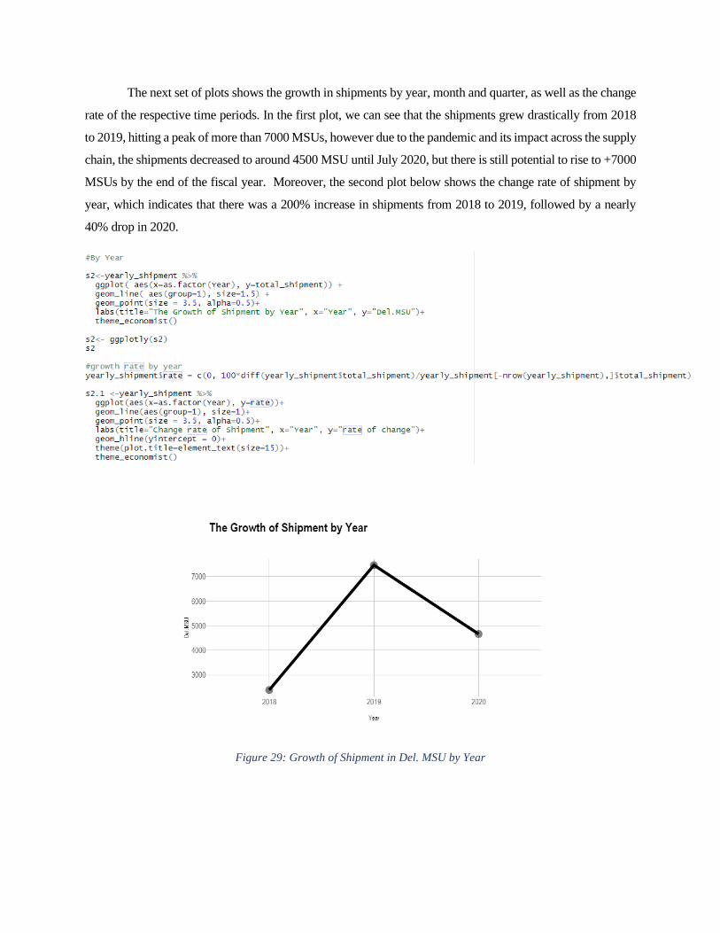
The next set of plots shows the growth in shipments by year, month and quarter, as well as the change

rate of the respective time periods. In the first plot, we can see that the shipments grew drastically from 2018

to 2019, hitting a peak of more than 7000 MSUs, however due to the pandemic and its impact across the supply

chain, the shipments decreased to around 4500 MSU until July 2020, but there is still potential to rise to +7000

MSUs by the end of the fiscal year. Moreover, the second plot below shows the change rate of shipment by

year, which indicates that there was a 200% increase in shipments from 2018 to 2019, followed by a nearly

40% drop in 2020.

Figure 29: Growth of Shipment in Del. MSU by Year

Figure 30: Change rate of Shipment in Del. MSU by Year

Similarly, the same plot is generated by quarter, where we can see a steady increase from Q1 to Q3,

followed by a drastic drop in Q4. After discussing with the Sales Logistics Leaders, this was found to be due

to the customers destocking to close their inventory on target, and hence ordering as per the sales forecast to

ensure that at the end of the year, they don’t start the next fiscal with excess cash held in inventory. The change

rate shown below shows a 20% increase in the shipments from Q1 to Q2, ~5% growth between Q2 and Q3,

followed by a drop of nearly 30% in Q4.

Figure 31: Growth of Shipment in Del. MSU by Quarter

Figure 32: Change rate of Shipment in Del. MSU by Quarter

The growth of shipment by month below shows a peak in March, however this is probably due to the

rise in shipments that happened in 2020 as we can see that the last two years did not follow the same trend,

followed by another peak in July due to the start of the fiscal year which is consistent across all years, and

finally, significant drops in June due to the destocking, and in August. The change rate fluctuates heavily across

the months, with significant drops in the rate of change between April and June, and finally in August. The

highest increase in rate of change is from August to September, with a growth rate of 75%.

Figure 33: Growth of Shipment in Del. MSU by Month

Figure 34: Change rate of Shipment in Del. MSU by Month

4.3 Forecasting Models

The next phase is applying the statistical and machine learning forecasting models to the dataset and

generating a plot of the forecast. We first begin with using the random walk, or the naïve methods, considering

the seasonality component, then moving on to exponential smoothing, ARIMA, linear and quadratic trend

models, Facebook Prophet, and finally machine learning methods including KNN and LSTM.

i. Naïve Models

The first plot below shows the forecast generated for the next 3 months using the naïve method. This

method assumes the last observed value for future forecasts, and hence is constant. This is evident from the

blue line where we can see a significant difference in the actual shipments vs. the forecast generated and

indicates that this is not a reliable forecast to use as it does not make any assumptions on trends or seasonality.

The snaïve forecast plot generates better results due to the seasonality component being factored in and provides

a good benchmark for the upcoming forecasting models.

Figure 35: Naïve Forecast Time Series Output

Figure 36: SNaïve Forecast Time Series Output

ii. Exponential Smoothing

The second forecasting method used is single exponential smoothing while allowing for a

multiplicative trend. This method gives weights to the data points, with the highest weights for the most recent

observations, and a decreasing weight given to historical observations. The forecast generated does not seem

accurate as it gives a relatively constant value, which is not in line with the actual shipments for the same period.

This indicates that exponential smoothing is probably not a good method to use for our dataset.

Figure 37: Exponential Smoothing Forecast Time Series Output

iii. Linear Trend Model

The third model used is the linear trend model, which is based on assuming a linear trend in the data

without any seasonal component and drawing a straight line of best fit to predict future values. As the dataset

on hand includes a seasonal component, a linear trend model does not look ideal to forecast the data as we can

see in the plot below, there are major differences in the forecast generated vs. the actual observed values.

Figure 38: Linear Trend Model Time Series Output

iv. Quadratic Trend Model

Similarly, a quadratic trend model was generated which takes into consideration one turning point in

the dataset and draws a quadratic line of best fit to predict future values. This is not considered a robust model

as it still does not consider the seasonality components in the dataset and gives equal weights to all datapoints.

Hence, we can conclude that this model is not the optimal one to forecast our time series.

Figure 39: Quadratic Trend Model Forecast Time Series Output

v. ARIMA

The first part of forecasting the time series using ARIMA is decomposing the additive series into the

observed, trend, seasonal and random components that make it up. We can see from the decomposition plot

below that there is a seasonality in the dataset which needs to be transformed prior to forecasting, as well as a

slight positive trend. The random variable component shows no trend in the residuals or noise data; however,

it is indicative of areas of variability with time with higher variability towards the end. After applying the first

difference to the dataset and generating the second plot below, we can see that the series achieved stationarity

after the first difference, which is confirmed by the Dickey Fullner test. Hence, the d value of the ARIMA

model is 1.

Figure 40: Time Series Decomposition Plot

Figure 41: Stationary Plot after first difference is applied

The next part is identifying the relevant p and q values of the ARIMA model using the ACF and PACF

plots. Although the autocorrelation plots give an indication on the parameters of the ARIMA model, it is quite

challenging to determine as it is subjective and based on the outcome of two plots, and still requires multiple

trial and error testing with different values for p and q and comparing the AIC to find the optimal ARIMA

model. The table below shows a guideline on how to determine p and q values for the AR and MA terms in

the case of a seasonal time-series (P,D,Q)m.

Table 11: Determining AR and MA values for ARIMA model

From the ACF plot below, we can see a fast decay towards the 0 mark with multiple significant lags,

suggesting an MA value of 1. Moreover, the PACF plot shows a geometric decay with a lag at approximately

every 6th point, indicating an AR value of 1 with a seasonal component and an m value of 6.

Figure 42: ACF Plot

Figure 43: PACF Plot

After running the model with ARIMA (1,1,1)(1,0,0)6, the output of the residuals shows a normal

distribution and no correlation or trend, however, the ACF plot had multiple spikes, indicating that this is not

the optimal model. Moreover, the Ljung-Box test checks the robustness of the model, where the null hypothesis

is the model is fit and the alternative being the model is not fit. From the output below, we can see that the null

hypothesis was rejected with p <0.05 and the model is not fit with an AIC value of 45.85.

Figure 44: Residual Plot for ARIMA(1,1,1)(1,0,0)[6]

The next step would be to run the auto.arima function to see if its in line with our expectations, and

compare the two models in terms of the AIC measure. The auto.arima function suggested an ARIMA model

with parameters (1,1,1) with seasonal as (1,0,0), with frequency equal to 30 observations per year. This was in

line with our expectations from the ACF and PACF plots above, however the frequency was taken at a higher

rate of 30 vs. the 6 suggested earlier. The evaluation metrics of this model order are AIC of 45.73, hence, we

can see that this is a better fit than the model above.

After multiple trials and errors to improve the accuracy of the fit, the optimal model was found to be

ARIMA (30,1,1)X(1,0,1)30, resulting in an AIC measure of 9.36. Below is the forecast generated using the

training dataset to predict the next 3 months compared to the actual observed values.

Figure 45: ARIMA (30,1,1)X(1,0,1)30 model forecast

The residuals from the model are displayed below, where they relfect a normal distribution centered around

the mean of 0, errors having a smaller range and the ACF plot relatively within the thresholds with one spike.

Figure 46: Residual Plots for ARIMA (30,1,1)(1,0,1)[30] model

vi. Facebook Prophet

The next model used is Facebook Prophet, where the model considers seasonality, trend, and certain

holiday events into the overall forecast. We can see that it closely captures the actual observed shipment values,

indicating that it could be an accurate model to use for the purpose of our time series models.

Figure 47: Facebook Prophet Forecast

vii. LSTM Forecasting

LSTM is a deep learning method using the basis of recurrent neural networks to build its architecture.

The plot below shows the forecast generated using the LSTM model and its comparison to the actual values

observed in the time series. We can see that it follows the same trends as the actual datapoints showing several

overlaps between the forecasted data points and the actual values, thus, indicating that it is a good fit to our

dataset and is competitive with the ARIMA and Facebook Prophet models. The evaluation metrics will be used

to have a conclusive decision on the optimal model and the ranks.

Figure 48: LSTM Seasonal Forecast

viii. KNN

Lastly, we look at KNN, STM is a deep learning method using the basis of recurrent neural networks

to build the architecture. Before consulting the training examples with knn_examples, we have to build the

model. This is done with the function knn_forecasting that builds a model associated with a time series and

uses the model to predict the future values of the time series. The result of the prediction is shown below and

is displayed on the plot.

Figure 49: KNN Forecast

4.4 Clustering and Market Basket Analysis

In this section, the outcome from the clustering analysis and market basket analysis will be discussed.

Cluster Analysis

For the cluster analysis, the k-means algorithm was used to cluster the SKUs with hopes of finding a

new proposal for the segmentation strategy which the SKUs can be based upon, in comparison the current

strategy used. After removing the unneeded columns and taking a sample of the dataset for faster computational

time and storage memory limitations, a summary was created for the remaining columns, as shown below. We

can see that the categorical variables are factors, indicating the need for one-hot encoding in preparation for

clustering.

From the total within and between sum of squares plots below, we can see that the optimal value of K

is 8, which is the point of deflection or the “elbow”. Another interpretation would be a K value of 3, hence, we

will try both and evaluate the performance of the clusters formed.

Figure 50: Total Within Sum of Squares

Figure 51: Total Between Sum of Squares

The cluster analysis was conducted with a K of 3, and the size of the clusters was 21,313, 27,378 and

66,575. We can see that the first two clusters are somehow equal in size, whereas the third cluster is nearly 3

times larger, indicating that the clusters are non-homogenous. This is also evident in the visual below, where

we can see that the clusters also overlap and are relatively loose, indicating that points may belong to more than

one cluster, which is not ideal for a segmentation proposal.

Figure 52: Cluster plot of K=3

The same analysis was repeated with a K value of 8, however there was a higher overlap between the

clusters and it was harder to visualize, hence for simplicity, we opted for the K value of 3.

Figure 53: Cluster plot of K=8

The results of the clustering analysis with K=3 is displayed below showing a snapshot of the means of each

cluster by variable.

Market Basket Analysis

After running the analysis on relative frequency for all the SKUs in the dataset, the top 10 SKUs which

were most frequently purchased are displayed below:

Figure 54: Top 10 most frequently bought items

Moreover, after applying the association rules using the apriori function, we took a subset of the rules

generated in the dataframe, and an example snapshot is shown below. We can see from the output below, that

for example, when customers purchase item 81665863, item 81579338 will be purchased where 50% of these

transactions contain these two products, as well as 100% certainty and a very high linkage between the two

SKUs due to the lift value of 2. The materials are displayed below.

After further analysis into the SKUs, It was found that the majority of the SKUs bought first are

bulky products that have a high vehicle fill rate and take up significant space when stacking and filling the

trucks, i.e. Fabric Care or Baby Care products frequently bought with the Hair Care SKUs. This indicates that

the Hair Care SKU (81579338) is a high selling SKU and has relatively much smaller dimensions used to fill

the remainder of the truck in to meet the vehicle fill rate threshold for shipments of 90% when customers

place orders.

Another example is shown below to answer the question of “What are customers likely to buy before

they purchase the Material 81579338?” We can see that the left-hand side of the equation contains all the SKUs

that customers are likely to buy, where 6.2% of the transactions contain these products. Moreover, a confidence

level of 1 indicates that it is certain that when the products on the left-hand side of the equation are purchased,

the item on the right-hand will be bought as well. The lift of 2 indicates that the presence of SKUs on the left,

increase the probability that the one on the right will occur in the transaction, hence, a greater link between the

two SKUs.

4.5 Evaluation

After creating the training and test set, building the classical time series models and the machine learning

models, the next step is to evaluate the performance of our forecasting models and conclude on the optimal one

to use in the time series forecast. As discussed in Chapter 3, the evaluation metrics to be used are the MAE and

RMSE for the forecasting models. Similarly, the performance of the clustering analysis done using k-means

method was evaluated using sum of squares. The chapter is split into two sections: Time Series Forecast

Evaluation and Clustering Evaluation.

Time Series Forecast Evaluation

The table below summarizes the evaluation metrics across the statistical and machine learning models

and their respective ranks based on their performance. The aim is to minimize both RMSE and MAE measures

to have a better fit model to predict future values. From the results, we can conclude that the SARIMA was the

optimal method with an RMSE of 0.25 and MAE of 0.18, which are both relatively close to 0 and indicating

an exceptionally low range of errors. This was followed by LSTM and ETS models, with the worst being the

naïve forecast that forms no prior assumptions on the dataset.

Table 12: Comparison of Evaluation Metrics for the Forecasting Models

Measure Naive Snaive ETS Linear Quadratic SARIMA Prophet KNN LSTM

RMSE 17.16 15.37 12.15 14.78 13.38 0.25 12.22 15.27 0.94

MAE 13.20 11.60 9.47 11.99 11.65 0.18 10.44 13.58 0.66

Rank 9 8 3 6 5 1 4 7 2

Overall, the results show that out of the machine learning techniques used, LSTM performed

significantly better than KNN. However, the statistical methods such as ETS and SARIMA generally

outperformed the machine learning alternatives. On the other hand, LSTM looks promising as it yielded

relatively accurate results, despite it known for performing better for long-term series and sequential data

compared to ARIMA which is better suited for forecasting in the short-term. Moreover, LSTM and KNN took

much longer to train the dataset and the computational time and power used was high compared to the statistical

alternatives which were able to generate an accurate forecast much quicker, hence, I would resort for SARIMA

as the optimal forecasting method in terms of its accuracy as well as computational speed and cost.

Clustering Evaluation

In comparison to supervised learning techniques, clustering does not use a solid metric that can clearly

evaluate the performance of the clustering algorithm. Moreover, since the algorithm depends on manually

choosing the optimal k instead of learning from the data, the elbow method is often used to choose the value of

k to minimize the sum of squares, and hence, for our case it was both 8 and 3. The within sum of squares in

each cluster is shown below, showing exceptionally large error values which is evident from the cluster plot in

Chapter 7, indicating large variability within a cluster. This is likely due to kmeans performing better with

clustering data that has a spherical shape around the center, whereas our dataset seems to display a rather more

wide and flat shape. Hence, kmeans could not identify the clusters accurately as it tries to minimize the within

cluster variation, and generally allocates a higher weight to bigger clusters than the smaller ones. Furthermore,

the total sum of squares was found to be 7,838,020, total within of 7,262,545 and total between was 575,475.

The % of between SS/total SS is 7.3%.

Although kmeans clustering is relatively simple and fast to implement, it has multiple drawbacks such

as needing to manually choose an optimal value of K and being sensitive to outliers given the dataset does not

have a spherical shape. Other clustering techniques such as hierarchal clustering and PAM should be

investigated and compared to against this method.

Chapter 5 – Conclusion

5.1 Conclusion

To summarize, forecasting demand is considered to be a fundamental exercise in any organization to

feed into and plan other internal cycles and processes such as production, procurement and generating sales

plans. The FMCG industry generates hundreds to thousands of transactions on a daily basis, adding more

complexity to demand planners in generating their forecasts in a robust and proactive manner. This brought the

attention of using big data analysis and forecasting methodologies to investigate the optimal method to use for

data within this industry. Machine learning time series models have gained considerable attention and

popularity in our current times behind the developments in AI, and hence have become worth studying in

comparison to classical forecasting methods. Moreover, generating an accurate forecast has become a necessity

for subsequent events, to ensure that inventory levels are optimized to reduce cash held in inventory, while

meeting market demand considering the volatility.

From the analysis conducted in this paper, we can conclude that generally, statistical methods tend to

outperform machine learning techniques where SARIMA and ETS models performed better than KNN.

However, it is worth noting that LSTM came close to SARIMA in terms of accuracy of the model fit and was

ranked second best, hence, looking at longer time horizons and generating forecasts for the next year can be

experimented on LSTM to validate its sensitivity to the forecasting horizon used. Furthermore, LSTM and ML

methods in general are known to perform better over longer time series data, and hence they can be used for

long term planning, while the statistical methods such as ARIMA can be used to forecast the short term. Using

SARIMA to create the forecasts for the FMCG for the next 3-month demand will generate significant benefits

in terms of inventory management, cash optimization as well as accuracy of capacity and raw material

procurement, whereas LSTM can be used for the long term in order to forecast capacity for the next year to

make decisions on capital investments or warehouse expansion.

For the second part of the study regarding the clustering analysis, the kmeans algorithm suggested a k

value of 3 as the optimal number of clusters, however with a significantly high sum of squares value. This does

not provide with a strong basis to formulate a product segmentation proposal, and other clustering techniques

would need to be explored before coming up with a final decision on how to simplify and improve the

categorization of products within the portfolio. Moreover, further data needs to be obtained on the entire SKU

portfolio and combined with sales data and unit cost to develop a comprehensive SKU segmentation strategy

that can be implemented within the forecasts and through inventory management.

5.2 Future Work

Although the provided analysis and methodology are quite sufficient to meet the requirements of the

FMCG company on hand, there are several factors that are worthy to consider for future investigations, as

summarized below:

• Gather more information about unknown future values instead of known ones to use as basis for

the optimization and fine-tuning to improve the current forecasting models used, especially for

ML methods

• Rather than depending on ML methods to make no assumptions regarding the seasonality and

trends, it is worth deseasonalizing the data before applying the techniques to lessen the

computational time needed to reach the optimal weights and generate forecasts faster to serve the

purpose of the organization

• Preprocessing and cleaning the data took the most significant time out of the entire process,

hence, a next step would be to automate the cleaning and pre-processing steps to avoid extra

decisions and efforts from the user

• Provide more insights on the construction of confidence intervals around ML forecasts and an

estimation of uncertainty around the forecasted values

• ML methods are known to overfit the data; hence, it would be advisable to avoid overfitting so

the models can correctly distinguish noise data from the trend and seasonality elements

• A next step would be to investigate a combined forecast approach, by feeding the forecasts

produced by the statistical methods to the ML model for each forecasting horizon and asking

them to choose the best one to minimize the errors. This would require clustering to be done on

the dataset and different models to be conducted for each cluster or type of series. The end in

mind would be finding a way to combine multiple forecasts to generate the optimal one

• Investigate other machine learning methodologies such as MLP, SVM/R and CART as

alternatives

• Re-run the analysis for a longer time-horizon and investigate the performance of the different

models accordingly. It is likely that the ML methods will outperform statistical ones in this area.

• Investigate further into the reasons behind the lower performance of machine learning methods

compared to statistical alternatives, as well as understand how the forecasts are being generated

• Look into other robust alternatives for k-means such as the Partition Around Medoids (PAM)

method, which is known to find observations from the original dataset that are closest to the

center of each cluster, as well as the silhouette plot to compare how close the datapoints are to

each other in their respective clusters

Bibliography

Adebanjo, D., & Mann, R. (2000). Identifying problems in forecasting consumer demand in the fast moving

consumer goods sector. Benchmarking: An International Journal, 7(3), 223-230. doi:

10.1108/14635770010331397

Albarune, A. R., & Habib, M. (2015). A Study of Forecasting Practices in Supply Chain Management.

International Journey of Supply Chain Management, 55-56.

Chu, C. and Zhang, G., 2003. A comparative study of linear and nonlinear models for aggregate retail

sales forecasting. International Journal of Production Economics, [online] 86(3), pp.217-231.

Available at: <https://www-sciencedirect-

com.ezproxy.rit.edu/science/article/pii/S0925527303000689> [Accessed 5 December 2020].

Cronshaw, N., 2018. Forecasting With Facebook's Prophet | Demand-Planning.Com. [online] Demand

Planning. Available at: <https://demand-planning.com/2018/03/14/forecasting-with-facebooks-

prophet/> [Accessed 5 December 2020].

Heinecke, G., Syntetos, A. and Wang, W., 2013. Forecasting-based SKU classification. International

Journal of Production Economics, 143(2), pp.455-462.

Holý, V., Sokol, O. and Černý, M., 2017. Clustering retail products based on customer behaviour. Applied

Soft Computing, 60, pp.752-762.

Huiskonen, J., 2001. Maintenance spare parts logistics: Special characteristics and strategic

choices. International Journal of Production Economics, 71(1-3), pp.125-133.

Iwok, I. and Okpe, A., 2016. A Comparative Study between Univariate and Multivariate Linear

Stationary Time Series Models. American Journal of Mathematics and Statistics, 6(5).

Jaipuria, S., & Mahapatra, S. (2014). An improved demand forecasting method to reduce bullwhip effect

in supply chains. Expert Systems With Applications, 41(5), 2395-2408. doi:

10.1016/j.eswa.2013.09.038

Ma, Y., Wang, N., Che, A., Huang, Y., & Xu, J. (2013). The bullwhip effect on product orders and

inventory: a perspective of demand forecasting techniques. International Journal Of Production

Research, 51(1), 281-302. doi: 10.1080/00207543.2012.676682

Mah, P. and Nanyan, N., 2020. A COMPARATIVE STUDY BETWEEN UNIVARIATE AND

BIVARIATE TIME SERIES MODELS FOR CRUDE PALM OIL INDUSTRY IN PENINSULAR

MALAYSIA. MALAYSIAN JOURNAL OF COMPUTING, 5(1), p.374.

Makridakis, S., Spiliotis, E., & Assimakopoulos, V. (2018). Statistical and Machine Learning forecasting

methods: Concerns and ways forward. PLOS ONE, 13(3), e0194889. doi:

10.1371/journal.pone.0194889

NEW REPORT: The Fast-Moving Consumer Goods Forecasting Evolution - Prevedere. (2017). Retrieved

2 May 2020, from https://www.prevedere.com/new-report-fast-moving-consumer-goods-forecasting-

evolution/

Ömer Faruk, D., 2010. A hybrid neural network and ARIMA model for water quality time series

prediction. Engineering Applications of Artificial Intelligence, 23(4), pp.586-594.

Park, J., Chang, B. and Mok, N., 2019. 144 Time Series Analysis and Forecasting Daily Emergency

Department Visits Utilizing Facebook's Prophet Method. Annals of Emergency Medicine, [online]

74(4), p.S57 [Accessed 5 December 2020].

Parmezan, A., Souza, V. and Batista, G., 2019. Evaluation of statistical and machine learning models for

time series prediction: Identifying the state-of-the-art and the best conditions for the use of each

model. Information Sciences, 484, pp.302-337.

Pereira Da Veiga, C., Pereira Da Veiga, C., Catapan, A., Tortato, U., & Da Silva, W. (2014). Demand

forecasting in food retail: a comparison between the HoltWinters and ARIMA models. International

Journal Of Production Economics, 11(3), 611-613.

Prudêncio, R., & Ludermir, T. (2005). Using machine learning techniques to combine forecasting methods.

(pp. 1122-1127). Berlin, Heidelberg: Springer Berlin Heidelberg.

Sezer, O., Gudelek, M. and Ozbayoglu, A., 2020. Financial time series forecasting with deep learning : A

systematic literature review: 2005–2019. Applied Soft Computing, 90, p.106181.

Vayvay, O., Dogan, O., & Ozel, S. (2013). FORECASTING TECHNIQUES IN FAST MOVING

CONSUMER GOODS SUPPLY CHAIN: A MODEL PROPOSAL. International Journal Of

Information Technology And Business Management, 15(1), 120-121. Retrieved from

https://www.researchgate.net/profile/Semih_Oezel/publication/289730222_Forecasting_Techniques

_in_Fast_Moving_Consumer_Goods_Supply_Chain_A_Model_Proposal/links/5692547808ae0f920

dcd5b6a/Forecasting-Techniques-in-Fast-Moving-Consumer-Goods-Supply-Chain-A-Model-

Proposal.pdf

Wang, P., Zheng, X., Li, J. and Zhu, B., 2020. Prediction of epidemic trends in COVID-19 with logistic

model and machine learning technics. Chaos, Solitons & Fractals, 139, p.110058.

Yang, B., Li, S., & Zhang, C. (2012). Research on Multilevel Inventory Control of FMCG Industry Based

on System Dynamics. Applied Mechanics And Materials, 157-158(3), 1212-1219. doi:

10.4028/www.scientific.net/amm.157-158.1212