comparative performance of different statistical … · comparative performance of different...
TRANSCRIPT

Comparative Performance of Different Statistical Models for Predicting
Ground-Level Ozone (O3) and Fine Particulate Matter (PM2.5) Concentrations
in Montréal, Canada
Edouard Philippe Martin
A Thesis
in
The Department
of
Building, Civil and Environmental Engineering
Presented in Partial Fulfillment of the Requirements
For the Degree of Master of Applied Science (Civil Engineering) at
Concordia University
Montréal, Québec, Canada
May 2011
© Edouard Philippe Martin, 2011

ii
CONCORDIA UNIVERSITY
School of Graduate Studies
This is to certify that the thesis prepared
By: Edouard Philippe Martin
Entitled: Comparative Performance of Different Statistical Models for
Predicting Ground-Level Ozone (O3) and
Fine Particulate Matter (PM2.5) Concentrations in Montréal, Canada
and submitted in partial fulfillment of the requirements for the degree of
Master of Applied Science (Civil Engineering)
complies with the regulations of the University and meets the accepted standards with
respect to originality and quality.
Signed by the final Examining Committee:
__________________________________________________ Chair
Dr. S. Li
__________________________________________________ Examiner
Dr. C. Mulligan
__________________________________________________ Examiner
Dr. M. Y. Chen
__________________________________________________ Supervisor
Dr. Z. Chen
Approved by ___________________________________
Dr. K. Ha-Huy, Graduate Program Director Department of Building, Civil and Environmental Engineering
__________ 2011 ___________________________________
R.A.L. Drew, Dean Faculty of Engineering and Computer Science

iii
ABSTRACT
Comparative Performance of Different Statistical Models for Predicting
Ground-Level Ozone (O3) and Fine Particulate Matter (PM2.5) Concentrations
in Montréal, Canada
Edouard Philippe Martin
Ground-level ozone (O3) and fine particulate matter (PM2.5) are two air pollutants known
to reduce visibility, to have damaging effects on building materials and adverse impacts
on human health. O3 is the result of a series of complex chemical reactions between
nitrogen oxides (NOx) and volatile organic compounds (VOCs) in the presence of solar
radiation. PM is a class of airborne contaminants composed of sulphate, nitrate,
ammonium, crustal components and trace amounts of microorganisms. PM2.5 is the
respirable subgroup of PM having an aerodynamic diameter of less than 2.5 μm.
Development of effective forecasting models for ground-level O3 and PM2.5 is important
to warn the public about potentially harmful or unhealthy concentration levels.
The objectives of this study is to investigate the applicability of Multiple Linear
Regression (MLR), Principle Component Regression (PCR), Multivariate Adaptive
Regression Splines (MARS), feed-forward Artificial Neural Networks (ANN) and hybrid
Principal Component – Artificial Neural Networks (PC-ANN) models to predict
concentrations of O3 and PM2.5 in Montréal (Canada). Air quality and meteorological
data is obtained from the Réseau de surveillance de la qualité de l’air (RSQA) for the
Airport Station (45°28′N, 73°44′W) and the Maisonneuve Station (45°30′N, 73°34′W) for
the period January 2004 to December 2007. Air pollution data include concentration

iv
values for nitrogen monoxide (NO), nitrogen dioxide (NO2), carbon monoxide (CO) and
142 different volatile organic compounds. Meteorological data include solar irradiation
(SR), temperature (Temp), pressure (Press), dew point (DP), precipitation (Precip), wind
speed (WS) and wind direction (WD).
Analysis of the available volatile organic compound data expressed on a
propylene-equivalent concentration indicated that m/p-xylene, toluene, propylene and
(1,2,4)-trimethylbenzene were species with the most significant ozone forming potential
in the study area.
Different models and architectures have been investigated through five case
studies. Predictive performances of each model have been measured by means of
performance metrics and forecast success rates. Overall, MARS models allowing second
order interaction of independent basis functions yielded lower error, higher correlation
and higher forecast success rates. This study indicates that models based on statistical
methods can be cost-effective tools to forecast ground-level O3 and PM2.5 in Montréal
and to provide support for decision makers in protecting human health.

v
AKNOWLEDGEMENTS
I would like to express my appreciation to my thesis supervisor, Dr. Zhi Chen, for his
guidance and continuous support throughout my graduate studies at Concordia
University. Dr. Chen taught me how to define and develop a research project. He has
encouraged me to investigate topics that interest me while providing timely suggestions
for improvement. I sincerely thank him for his patience during the time it took me to
write this thesis.
I take this opportunity to knowledge Dr. John Hadjinicolaou, who has marked my
academic journey with his insatiable questioning of why (and how) things are the way
they are. I would like to thank Mr. Conrad Lapensée and Mme. Rodica Motora: they
taught me more than calculus and linear algebra in high school, they taught me logic and
critical thinking.
I extend my gratitude to Mr. Claude Gagnon (Réseau de Surveillance de la
Qualité de l'Air de Montréal) for providing the data for this thesis, and the whole team at
Salford Systems (San Diego, California, USA) for providing the “Salford Predictive
Miner” software.

vi
To my wife Deniz
Aos meus pais e aos meus irmãos e à toda minha familia
In the hope that others will continue and improve on this work...

vii
TABLE OF CONTENTS
List of Figures xi
List of Tables xv
List of Symbols xxii
List of Abbreviations and Acronyms xxv
Chapter 1 Introduction 1
1.1 Background . . . . . . . . . . . . . . . . . . . . . . . 1
1.2 Objective and Scope of This Study . . . . . . . . . . . . 5
1.3 Methodology . . . . . . . . . . . . . . . . . . . . . . . 6
1.4 Value of Results and Contribution to Research . . . . . . . . . . 7
1.5 Organisation of this Thesis . . . . . . . . . . . . . . . . . . 8
Chapter 2 Literature Review 10
2.1 Earth’s Atmosphere . . . . . . . . . . . . . . . . . . . . 10
2.2 Ozone (O3) . . . . . . . . . . . . . . . . . . . . . . . . 13
2.3 Particulate Matter (PM) . . . . . . . . . . . . . . . . . . . 19
2.4 Influence of Meteorology on O3 and PM . . . . . . . . . . . . 23
2.5 Impact of O3 and PM on Human Health . . . . . . . . . . . . . 25
2.6 Air Quality Standards for O3 and PM . . . . . . . . . . . . . . 30
2.7 Statistical Models used in O3 and PM Forecasting . . . . . . . . . 33
2.8 Discussion . . . . . . . . . . . . . . . . . . . . . . . . 41
2.9 Summary . . . . . . . . . . . . . . . . . . . . . . . . . 48
Chapter 3 Methods and Performance Metrics 51
3.1 Preliminaries . . . . . . . . . . . . . . . . . . . . . . . . 51
3.1.1 Conventions . . . . . . . . . . . . . . . . . . . . 51
3.1.2 Time Series Data . . . . . . . . . . . . . . . . . . 52
3.1.3 Moment Statistics and Other Measurements . . . . . . . . 53
3.1.4 Principal Component Analysis (PCA) . . . . . . . . . . 55
3.2 Methods . . . . . . . . . . . . . . . . . . . . . . . . . . 59

viii
3.2.1 Multiple Linear Regression (MLR) . . . . . . . . . . . 62
3.2.2 Principal Component Regression (PCR) . . . . . . . . . 65
3.2.3 Multivariate Adaptive Regression Splines (MARS) . . . . . 66
3.2.4 Artificial Neural Networks (ANN) . . . . . . . . . . . 69
3.3 Performance Metrics . . . . . . . . . . . . . . . . . . . . 73
3.4 Discussion . . . . . . . . . . . . . . . . . . . . . . . . 76
3.5 Summary . . . . . . . . . . . . . . . . . . . . . . . . . 83
Chapter 4 Investigation Area and Data 86
4.1 Investigation Area . . . . . . . . . . . . . . . . . . . . . 86
4.2 Data Collection and Quality Analysis . . . . . . . . . . . . . . 90
4.3 Data Characterization . . . . . . . . . . . . . . . . . . . . 92
4.4 Diurnal Cycles . . . . . . . . . . . . . . . . . . . . . . . 107
4.5 Dataset Preparation . . . . . . . . . . . . . . . . . . . . . 117
Chapter 5 Results 119
5.1 Case Study 1: O3 Forecast at Airport Station . . . . . . . . . . . 119
5.1.1 Summer . . . . . . . . . . . . . . . . . . . . . . 119
5.1.2 Winter . . . . . . . . . . . . . . . . . . . . . . 125
5.2 Case Study 2: PM2.5 Forecast at Airport Station . . . . . . . . . . 128
5.2.1 Summer . . . . . . . . . . . . . . . . . . . . . 128
5.2.2 Winter . . . . . . . . . . . . . . . . . . . . . . 133
5.3 Case Study 3: O3 Forecast at Maisonneuve Station . . . . . . . . . 136
5.3.1 Summer . . . . . . . . . . . . . . . . . . . . . . 136
5.3.2 Winter . . . . . . . . . . . . . . . . . . . . . . 139
5.4 Case Study 4: PM2.5 Forecast at Maisonneuve Station . . . . . . . 142
5.4.1 Summer . . . . . . . . . . . . . . . . . . . . . . 142
5.4.2 Winter . . . . . . . . . . . . . . . . . . . . . . 145
5.5 Case Study 5: Daily O3 at Maisonneuve Station and VOC Data . . . 148
5.6 Comparison to Literature Data . . . . . . . . . . . . . . . . 154
5.7 Summary . . . . . . . . . . . . . . . . . . . . . . . . . 157
ix
Chapter 6 Conclusion 160
6.1 Conclusions . . . . . . . . . . . . . . . . . . . . . . . . 160
6.2 Recommendations for Future Work . . . . . . . . . . . . . . 163
Reference 165
Appendix A Derivation of the Gradient Descent Rule
Using the Sigmoid Activation Function 179
Appendix B Numerical Examples 182
B.1 A Numerical Example for Principal Component Analysis . . . . . . 182
B.2 A Numerical Example for Artificial Neural Network using
the Gradient Descent Rule and Sigmoid Activation Function . . . . . 196
Appendix C Completeness of the Data 201
Appendix D Monthly Averages (2004 – 2007 Time Series) 204
D.1 Air Quality at Airport . . . . . . . . . . . . . . . . . . . . 204
D.2 Air Quality at Maisonneuve . . . . . . . . . . . . . . . . . 205
D.3 Meteorological Data at Airport . . . . . . . . . . . . . . . . 206
Appendix E Typical Monthly Averages Observed in
2004 – 2007 Time Series 207
E.1 Air Quality at Airport . . . . . . . . . . . . . . . . . . . . 207
E.2 Air Quality at Maisonneuve . . . . . . . . . . . . . . . . . 207
E.3 Meteorological Data at Airport . . . . . . . . . . . . . . . . 208
Appendix F Hourly Averages (2004 – 2007 Time Series) by Season 209
Appendix G O3 and PM2.5 Averages at Airport and Maisonneuve
by Wind Direction (2004 – 2007 Time Series) 212

x
Appendix H Hourly Averages by Season by Period (2004 – 2007 Time Series)
213
H.1 Summer . . . . . . . . . . . . . . . . . . . . . . . . . . 213
H.2 Winter . . . . . . . . . . . . . . . . . . . . . . . . . . 217
Appendix I Sample Model Outputs for Case Study 1 (Day Period) 220
Appendix J Sample Error Diagnostics for Case Study 1 (Day Period) 229

xi
List of Figures
Figure 2.1 Earth’s atmosphere (Seinfeld and Pandis, 1998) . . . . . 11
Figure 2.2 Human respiratory system (HCEC 1998). . . . . . . . 28
Figure 3.1 Artificial Neural Network architecture . . . . . . . . . 71
Figure 4.1 Map of Canada (HRSDC, 2004) . . . . . . . . . . . 86
Figure 4.2 Population densities in Montréal (City of Montréal, 2003) . 88
Figure 4.3 RSQA Monitoring Stations in Montréal, adapted from
(RSQA, 2007). . . . . . . . . . . . . . . . . . . 89
Figure 4.4 Monthly means of O3 at Airport and Maisonneuve stations . 93
Figure 4.5 Monthly means of O3 at Airport and Maisonneuve stations
by month . . . . . . . . . . . . . . . . . . . . 93
Figure 4.6 Monthly means of PM2.5 at Airport and Maisonneuve stations 94
Figure 4.7 Monthly means of PM2.5 at Airport and Maisonneuve stations
by month . . . . . . . . . . . . . . . . . . . . 94
Figure 4.8 Monthly means of NO at Airport and Maisonneuve stations 96
Figure 4.9 Monthly means of NO at Airport and Maisonneuve stations
by month . . . . . . . . . . . . . . . . . . . . 96
Figure 4.10 Monthly means of NO2 at Airport and Maisonneuve stations 97
Figure 4.11 Monthly means of NO2 at Airport and Maisonneuve stations
by month . . . . . . . . . . . . . . . . . . . . 97

xii
Figure 4.12 Monthly means of CO at Airport and Maisonneuve stations 99
Figure 4.13 Monthly means of CO at Airport and Maisonneuve stations
by month . . . . . . . . . . . . . . . . . . . . 99
Figure 4.14 Monthly means of SR at Airport station . . . . . . . . . 100
Figure 4.15 Monthly means of SR at Airport station by month . . . . 100
Figure 4.16 Monthly means of Temp at Airport station . . . . . . . 101
Figure 4.17 Monthly means of Temp at Airport station by month . . . 101
Figure 4.18 Monthly means of DP at Airport station . . . . . . . . 102
Figure 4.19 Monthly means of DP at Airport station by month . . . . 102
Figure 4.20 Monthly means of Press at Airport station . . . . . . . . 103
Figure 4.21 Monthly means of Press at Airport station by month . . . . 103
Figure 4.22 Monthly means of Precip at Airport station . . . . . . . 104
Figure 4.23 Monthly means of Precip at Airport and stations by month . 104
Figure 4.24 WDI and maximum 1-hour O3 at Airport station by WD . . 106
Figure 4.25 WDI and maximum 1-hour O3 at Maisonneuve station by WD 107
Figure 4.26 Diurnal cycle of O3, PM2.5, NO, NO2 and CO (in μg/m3)
at Airport station (Summer) . . . . . . . . . . . . . 108
Figure 4.27 Diurnal cycle of O3, PM2.5, NO, NO2 and CO (in μg/m3)
at Airport station (Winter)) . . . . . . . . . . . . . 108
Figure 4.28 Diurnal cycle of O3, PM2.5, NO, NO2 and CO (in μg/m3)
at Maisonneuve station (Summer) . . . . . . . . . . . 109

xiii
Figure 4.29 Diurnal cycle of O3, PM2.5, NO, NO2 and CO (in μg/m3)
at Maisonneuve station (Winter) . . . . . . . . . . 109
Figure 4.30 Diurnal cycle of Temp and DP (oC); and Press (kPa)
at Airport station (Summer) . . . . . . . . . . . . 110
Figure 4.31 Diurnal cycle of Temp and DP (oC); and Press (kPa)
at Airport station (Winter) . . . . . . . . . . . . . 110
Figure 4.32 Diurnal cycle of Precip (mm) and SR (W/m2)
at Airport station (Summer) . . . . . . . . . . . . 111
Figure 4.33 Diurnal cycle of Precip (mm) and SR (W/m2)
at Airport station (Winter) . . . . . . . . . . . . . 111
Figure B.1 Roots of the characteristic equation . . . . . . . . . . 188
Figure J.1 Residual Moments (MLR, PCR) . . . . . . . . . . . 229
Figure J.2 Plot O3 observed by O3 predicted (MLR) in μg/m3 . . . . 230
Figure J.3 Plot Residual by O3 predicted (MLR) in μg/m3 . . . . . 230
Figure J.4 Plot O3 observed by O3 predicted (PCR) in μg/m3 . . . . 231
Figure J.5 Plot Residual by O3 predicted (PCR) in μg/m3 . . . . . 231
Figure J.6 Residual Moments (MARS 1, MARS 2) . . . . . . . . 232
Figure J.7 Plot O3 observed by O3 predicted (MARS 1) in μg/m3 . . 233
Figure J.8 Plot Residual by O3 predicted (MARS 1) in μg/m3 . . . . 233
Figure J.9 Plot O3 observed by O3 predicted (MARS 2) in μg/m3 . . . 234
Figure J.10 Plot Residual by O3 predicted (MARS 2) in μg/m3 . . . . 234
Figure J.11 Residual Moments (ANN, PC-ANN) . . . . . . . . . 235
Figure J.12 Plot O3 observed by O3 predicted (ANN) in μg/m3 . . . . 236

xiv
Figure J.13 Plot Residual by O3 predicted (ANN) in μg/m3 . . . . . 236
Figure J.14 Plot O3 observed by O3 predicted (PC-ANN) in μg/m3 . . 237
Figure J.15 Plot Residual by O3 predicted (PC-ANN) in μg/m3 . . . . 237
Figure J.16 Residual Moments (PC*-ANN) . . . . . . . . . . . . 238
Figure J.17 Plot O3 observed by O3 predicted (PC*-ANN) in μg/m3 . . 239
Figure J.18 Plot Residual by O3 predicted (PC*-ANN) in μg/m3 . . . . 239

xv
List of Tables
Table 2.1 Residency time and transport distance versus PM particle
size (Patel, 2004) . . . . . . . . . . . . . . . . . 25
Table 2.2 Summary of O3 impacts on human health . . . . . . . 27
Table 2.3 Summary of PM2.5 effect on human health . . . . . . . 27
Table 2.4 Existing air quality objectives, standards and guidelines
in Montréal, Canada and United States . . . . . . . . 33
Table 4.1 Montréal 30-year (1971-2000) temperature averages
(EC, 2011) . . . . . . . . . . . . . . . . . . . 87
Table 4.2 Montréal 30-year (1971-2000) rainfall, snowfall and
precipitation averages (EC, 2011) . . . . . . . . . . . 87
Table 4.3 Correlation of variables (Summer / Day) . . . . . . . . 115
Table 4.4 Correlation of variables (Summer / Night) . . . . . . . 115
Table 4.5 Correlation of variables (Winter / Day) . . . . . . . . 116
Table 4.6 Correlation of variables (Winter / Night) . . . . . . . . 116
Table 4.7 Learning and testing counts . . . . . . . . . . . . . . 118
Table 5.1 Forecasting summer O3 at Airport with PCR and MARS 1
(Training) . . . . . . . . . . . . . . . . . . . . 122

xvi
Table 5.2 Forecasting summer O3 at Airport with MLR, MARS 2 and
ANN (Training) . . . . . . . . . . . . . . . . . . 122
Table 5.3 Forecasting summer O3 at Airport with PC-ANN and
PC*-ANN (Training) . . . . . . . . . . . . . . . . 122
Table 5.4 Forecasting summer O3 at Airport with PCR and MARS 1
(Validation) . . . . . . . . . . . . . . . . . . . . 123
Table 5.5 Forecasting summer O3 at Airport with MLR, MARS 2 and
ANN (Validation) . . . . . . . . . . . . . . . . . 123
Table 5.6 Forecasting summer O3 at Airport with PC-ANN and PC*-ANN
(Validation) . . . . . . . . . . . . . . . . . . . . 123
Table 5.7 Forecasting winter O3 at Airport with MLR, MARS 2 and ANN
(Training) . . . . . . . . . . . . . . . . . . . . 127
Table 5.8 Forecasting winter O3 at Airport with MLR, MARS 2 and ANN
(Validation) . . . . . . . . . . . . . . . . . . . . 127
Table 5.9 Forecasting summer PM2.5 at Airport with PCR and MARS 1
(Training) . . . . . . . . . . . . . . . . . . . . 131
Table 5.10 Forecasting summer PM2.5 at Airport with MLR, MARS 2 and
ANN (Training) . . . . . . . . . . . . . . . . . . 131
Table 5.11 Forecasting summer PM2.5 at Airport with PC-ANN and
PC*-ANN (Training) . . . . . . . . . . . . . . . . . 131
Table 5.12 Forecasting summer PM2.5 at Airport with PCR and MARS 1
(Validation) . . . . . . . . . . . . . . . . . . . 132

xvii
Table 5.13 Forecasting summer PM2.5 at Airport with MLR, MARS 2 and
ANN (Validation) . . . . . . . . . . . . . . . . . . 132
Table 5.14 Forecasting summer PM2.5 at Airport with PC-ANN and
PC*-ANN (Validation) . . . . . . . . . . . . . . . . 132
Table 5.15 Forecasting winter PM2.5 at Airport with MLR, MARS 2 and
ANN (Training) . . . . . . . . . . . . . . . . . . 135
Table 5.16 Forecasting winter PM2.5 at Airport with MLR, MARS 2 and
ANN (Validation) . . . . . . . . . . . . . . . . . 135
Table 5.17 Forecasting summer O3 at Maisonneuve with MLR, MARS 2
and ANN (Training) . . . . . . . . . . . . . . . . 138
Table 5.18 Forecasting summer O3 at Maisonneuve with MLR, MARS 2
and ANN (Validation) . . . . . . . . . . . . . . . . 138
Table 5.19 Forecasting winter O3 at Maisonneuve with MLR, MARS 2 and
ANN (Training) . . . . . . . . . . . . . . . . . . . 141
Table 5.20 Forecasting winter O3 at Maisonneuve with MLR, MARS 2 and
ANN (Validation) . . . . . . . . . . . . . . . . . . 141
Table 5.21 Forecasting summer PM2.5 at Maisonneuve with MLR, MARS 2
and ANN (Training) . . . . . . . . . . . . . . . . . 144
Table 5.22 Forecasting summer PM2.5 at Maisonneuve with MLR, MARS 2
and ANN (Validation) . . . . . . . . . . . . . . . . 144
Table 5.23 Forecasting winter PM2.5 at Maisonneuve with MLR, MARS 2
and ANN (Training) . . . . . . . . . . . . . . . . 147
xviii
Table 5.24 Forecasting winter PM2.5 at Maisonneuve with MLR, MARS 2
and ANN (Validation) . . . . . . . . . . . . . . . 147
Table 5.25 VOC species at Maisonneuve ranked by ppbC
(KOH from Atkinson (1990)) . . . . . . . . . . . . . 149
Table 5.26 VOC species at Maisonneuve ranked by propy-equiv ppbC
(KOH from Atkinson (1990)) . . . . . . . . . . . . . 149
Table 5.27 Predicting O3 at Maisonneuve with MLR, MARS 2 and ANN
including VOC data (Training) . . . . . . . . . . . . 152
Table 5.28 Predicting O3 at Maisonneuve with MLR, MARS 2 and ANN
including VOC data (Validation) . . . . . . . . . . . . 152
Table 5.29 Performance of O3 forecasting methods from other studies 154
Table 5.30 Performance of PM2.5 forecasting methods from other studies 154
Table B.1 Data for matrix X in PCA numerical example . . . . . . 182
Table B.2 Data for matrix Z in PCA numerical example. . . . . . 184
Table B.3 Data for matrix S in PCA numerical example. . . . . . 186
Table B.4 False Position Method iterations for λ1 in PCA numerical example 191
Table B.5 False Position Method iterations for λ2 in PCA numerical example 192
Table B.6 False Position Method iterations for λ3 in PCA numerical example 192
Table B.7 Data for matrix F in PCA numerical example. . . . . . . . 195
Table B.8 Data for matrix X in ANN numerical example . . . . . . 196
Table B.9 Internal energies at first iteration in ANN numerical example . 198
Table B.10 Weight correction up to 10 iterations in ANN numerical example 200

xix
Table C.1 Completeness of the data for air pollution readings at
Airport station . . . . . . . . . . . . . . . . . . 201
Table C.2 Completeness of the data for air pollution readings at
Maisonneuve station . . . . . . . . . . . . . . . . 202
Table C.3 Completeness of the data for meteorological readings at
Airport station . . . . . . . . . . . . . . . . . . 203
Table D.1 Monthly averages (2004 – 2007) of air quality data at
Airport . . . . . . . . . . . . . . . . . . . . . . 204
Table D.2 Monthly averages (2004 – 2007) of air quality data at
Maisonneuve . . . . . . . . . . . . . . . . . . . 205
Table D.3 Monthly averages (2004 – 2007) of meteorological data at
Airport . . . . . . . . . . . . . . . . . . . . . 206
Table E.1 Averages by month of air quality data at Airport . . . . . 207
Table E.2 Averages by month of air quality data at Maisonneuve . . 207
Table E.3 Averages by month of meteorological data at Airport 208
Table F.1 Hourly averages of air quality data at Airport (Summer) 209
Table F.2 Hourly averages of air quality data at Airport (Winter) 209
Table F.3 Hourly averages of air quality data at Maisonneuve (Summer) 210
Table F.4 Hourly averages of air quality data at Maisonneuve (Winter) 210
Table F.5 Hourly averages of meteorological data at Airport (Summer) 211
Table F.6 Hourly averages of meteorological data at Airport (Winter) 211
Table G.1 O3 and PM2.5 Averages by Wind Direction . . . . . . . 212
Table H.1 Hourly averages of air quality data at Airport (summer/day) 213

xx
Table H.2 Hourly averages of air quality data at Maisonneuve (summer/day) 214
Table H.3 Hourly averages of meteorological data at Airport (summer/day) 215
Table H.4 Hourly averages of air quality data at Airport (summer/night) 215
Table H.5 Hourly averages of air quality data at Maisonneuve (summer/night) 216
Table H.6 Hourly averages of meteorological data at Airport (summer/night) 216
Table H.7 Hourly averages of air quality data at Airport (winter/day) 217
Table H.8 Hourly averages of air quality data at Maisonneuve (winter/day) 217
Table H.9 Hourly averages of meteorological data at Airport (winter/day) 218
Table H.10 Hourly averages of air quality data at Airport (winter/night) 218
Table H.11 Hourly averages of air quality data at Maisonneuve (winter/night) 219
Table H.12 Hourly averages of meteorological data at Airport (winter/night) 219
Table I.1 Model output MLR . . . . . . . . . . . . . . . . 220
Table I.2 Model output PCA . . . . . . . . . . . . . . . . 220
Table I.3 Model output PCR . . . . . . . . . . . . . . . . 221
Table I.4 Model identification MARS 1 . . . . . . . . . . . 222
Table I.5 Model output MARS 1 . . . . . . . . . . . . . . 223
Table I.6 Model identification MARS 2 . . . . . . . . . . . . 224
Table I.7 Model output MARS 2 . . . . . . . . . . . . . . . 225
Table I.8 Model identification ANN . . . . . . . . . . . . . 226
Table I.9 Model output ANN . . . . . . . . . . . . . . . . 226
Table I.10 Model identification PC-ANN . . . . . . . . . . . 227
Table I.11 Model output PC-ANN . . . . . . . . . . . . . . 227

xxi
Table I.12 Model identification PC*-ANN . . . . . . . . . . . 228
Table I.13 Model output PC*-ANN . . . . . . . . . . . . . . 228

xxii
List of Symbols
A Number of correctly predicted exceedances
BFi Generic basis function
c Generic knot in BFi
cp Penalty factor
d Effective degrees of freedom
e Model residual
E System overall energy
f Generic activation function
fsig Sigmoid activation function
i Generic index, i = {1, 2, 3, ... , n}
F Number of predicted exceedances
I Identity matrix
KOH OH-reactivity
L Diagonal matrix
Lss Sum of squares matrix
M Number of observed exceedances
n Number of observation
p Number of independent variables
q Number of hidden nodes
r Sample correlation coefficient

xxiii
R2 Coefficient of determination
s Sample standard deviation
𝑠2 Sample variance
Sy Variance matrix of matrix Y
Sz Variance matrix of matrix Z
t Time of observation
u1 Column vector
v1 First column vector of matrix V
V Orthonormal matrix
w Weight of hidden node
𝑤� Estimate of w through the Gradient descent rule
x Generic independent variable
�̅� Mean of x
X Matrix of generic independent variables
y Generic dependent variable
𝑦� Predicted value of y
�̇� Geometric mean
yT Power transform of y
yT* Scaled yT
Z Matrix of autoscaled generic independent variables
α Multiplier in hidden layer output
𝛽 Independent variable coefficient in a regression based model
�̂� Ordinary Least Square estimate of coefficient β

xxiv
ε Random error in a regression based model
λ Eigenvalue
𝜂 Learning rate
𝜑 Level of power transform
θ Constant in hidden layer output
θw Wind direction
ψ Phase shift parameter

xxv
List of Abbreviations and Acronyms
ANN Artificial Neural Network
CI Confidence Interval
CWS Canada Wide Standards
EC Environment Canada
FPR False Positive Rate
GVC Generalized Cross Validation
MAE Mean Absolute Error
MAPE Mean Absolute Percent Error
MARS Multivariate Adaptive Regression Splines
MLR Multiple Linear Regression
NAPS National Air Pollution Surveillance
OLS Ordinary Least Squate
PC Principal Components
PCA Principal Component Analysis
PCR Principal Component Regression
RMSE Root Mean Squared Error
SE Standard Error
SI Success Index
SR Solar Radiation

xxvi
TPR True Positive Rate
WD Wind Direction
WDI Wind Direction Index
WGAQOG Working Group on Air Quality Objectives and Guidelines

1
Chapter 1
Introduction
1.1 Background
In Canada, both the public and private sectors have a long track record in developing
strategies to control air pollution. Despite the coordinated implementation of these
strategies and advances in technology over the past years, ozone and particulate matter
are still prevalent in Eastern Canada (Brook and Dann, 2002). Because these two air
pollutants are known to reduce visibility, to have damaging effects on building materials
and to have adverse impacts on human health (Seinfeld and Pandis, 1998), they remain
important areas of concern for the scientific and engineering communities.
Ground-level ozone is the result of a series of complex chemical reactions
between precursor species, namely nitrogen oxides (NOx) and volatile organic
compounds (VOCs) in the presence of solar radiation (Nazaroff and Alvarez-Cohen,
2001).
Particulate matter is an intricate mixture of solid and liquid chemical elements,
organic compounds and biological species that vary in size and remain suspended in the

2
air. Precursor species to particulate matter are known to include NOx, VOCs, sulphur
dioxide (SO2) and ammoniac (NH3) (Stanier, 2003).
While ozone and particulate matter are a common problem to almost all major
cities in Eastern Canada, the magnitude of the problem varies regionally and locally.
Development of effective forecasting models at the local level to predict concentrations
of ozone and particulate matter is important because the information provided allows
people within a community to take precautionary measures to avoid or limit their
exposure to unhealthy levels of air quality (Karatzas and Kaltsatos, 2007).
Air pollution forecasting strategies can be divided in two broad categories:
deterministic and statistical. In deterministic models, prior knowledge about the
underlying chemical and physical processes governing air pollution is described by
means of differential equations with boundary condition (Liu, 2007). Statistical
models are more pragmatic mathematical descriptions of how the data can
conceivably be produced. Statistical models are used to a greater extent at trend
estimation and to a lesser degree at elucidating underlying mechanisms.
Deterministic models are commonly divided in three broad categories,
namely: Gaussian, Lagrangian and Eulerian models (Su, 2004). A number of
working deterministic platforms have been developed for air pollution monitoring,
namely the “Regional Climate Model” (Caya et al., 1995), the “Multiscale Air
Quality Simulation Platform” (Odman and Ingram, 1996), the “Goddard Earth
Observing System-Chemistry” (Garner et al., 2005) and the “Global Environmental
Multi-Scale - Modelling Air Quality and Chemistry” (Talbot et al., 2008), which is
3
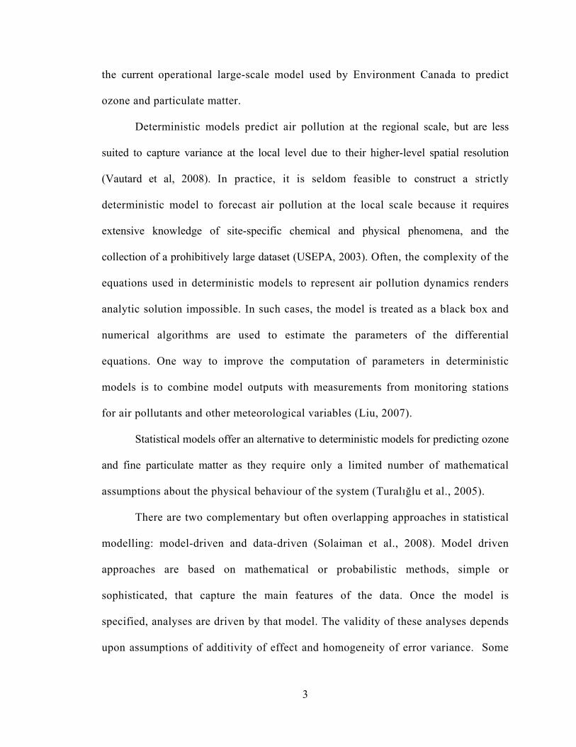
the current operational large-scale model used by Environment Canada to predict
ozone and particulate matter.
Deterministic models predict air pollution at the regional scale, but are less
suited to capture variance at the local level due to their higher-level spatial resolution
(Vautard et al, 2008). In practice, it is seldom feasible to construct a strictly
deterministic model to forecast air pollution at the local scale because it requires
extensive knowledge of site-specific chemical and physical phenomena, and the
collection of a prohibitively large dataset (USEPA, 2003). Often, the complexity of the
equations used in deterministic models to represent air pollution dynamics renders
analytic solution impossible. In such cases, the model is treated as a black box and
numerical algorithms are used to estimate the parameters of the differential
equations. One way to improve the computation of parameters in deterministic
models is to combine model outputs with measurements from monitoring stations
for air pollutants and other meteorological variables (Liu, 2007).
Statistical models offer an alternative to deterministic models for predicting ozone
and fine particulate matter as they require only a limited number of mathematical
assumptions about the physical behaviour of the system (Turalığlu et al., 2005).
There are two complementary but often overlapping approaches in statistical
modelling: model-driven and data-driven (Solaiman et al., 2008). Model driven
approaches are based on mathematical or probabilistic methods, simple or
sophisticated, that capture the main features of the data. Once the model is
specified, analyses are driven by that model. The validity of these analyses depends
upon assumptions of additivity of effect and homogeneity of error variance. Some

4
inferences are strictly valid under further assumptions of normality of residuals. The
majority of model-driven approaches are in some sense regression-based, with
varying degrees of complexity (Thompson et al., 2001). Model-driven methods
include Multiple Linear Regression, Nonlinear Regression, Piecewise Regression
and Quantile Regression. Data-driven approaches comprise of analytic processes
designed to explore data in search of consistent patterns and/or systematic
relationships between variables without an explicit model characterization
(Solaiman et al., 2008). Data-driven models are also to a great extent user-centric
and interactive processes which leverage analysis technologies and machine
computing power. Data-driven methods include Classification and Regression
Trees, Cluster Analysis, Fuzzy Inference Systems, Artificial Neural Networks,
Bayesian Networks and Multivariate Adaptive Regression Splines.
Over the years, a number of statistical approaches, both model and data
driven, have been proposed to forecast ground-level ozone and particulate matter.
Despite their evident useful contributions, no a priori conclusion can be drawn with
respect to their overall performance considering different geographic locations and
meteorological conditions (Sousa et al., 2007). In other words, conclusions drawn
from a specific study cannot be extrapolated to other sites due to area specificities.
Only through model development and performance assessment can we conclude
which model is best suited for a specific location.
To this date, no comparative assessment of different statistical models for
short-term prediction of ground level ozone and particulate matter in Montréal
(Canada) has been undertaken.

5
While public health imperative provides one motivation for this study, the
challenge of developing accurate air pollution forecasting models provides another.
1.2 Objectives and Scope of This study
The main purpose of this study is to gain understanding of air quality and how
concentration levels of air pollutants can be forecasted. In order to investigate this,
the thesis takes its analytic departure in an extensive amount of empirical data. The
data consist of four years of air quality and meteorological data. In this way, we
analyse and incorporate both chemical and physical measurements.
The objectives of this study are to determine seasonal and diurnal patterns of
ground-level ozone (O3) and fine particulate matter (PM2.5); to investigate the ozone
forming potential of different volatile organic compound species in the city and to
assess the suitability of different statistical methods for short-term forecast.
The reason for focusing on ozone and fine particulate matter (rather than any
other known air pollutants) stems from the fact that O3 and PM2.5 are secondary air
pollutants (i.e. not emitted from sources) and highly dependent of precursor species
and meteorological conditions.
The study area is limited to the most densely populated areas of Montréal.
The air quality and meteorological data used in this thesis has been measured and
validated by the Réseau de surveillance de la qualité de l'air (RSQA) for the period
covering January 2004 to December 2007, inclusively.

6
Data processing, statistical analysis and model development has been carried
out using two commercially available statistical softwares, namely “Salford Predictive
Miner” from Salford Systems (San Diego, CA, USA) and “JMP Version 5.1.2” from SAS
Institute Inc. (Cary, NC, USA).
1.3 Methodology
The proposed methodology comprises the following eight steps:
1. Review the chemical and physical processes involved in the formation of ozone
and particulate matter;
2. Identify the potential air pollution and meteorological variables for building
prediction models;
3. Obtain relevant data covering a representative period of time;
4. Develop different predictive models based on statistical methods;
5. Define an appropriate set of performance metrics;
6. Assess each model in terms of performance metrics;
7. Determine the best model for short-term forecasting of ozone and particulate
matter; and
8. Gauge the performance the developed models in comparison to literature
data.

7
1.4 Value of Results and Contribution to Research
This work contributes to research by a) increasing domain knowledge related to
secondary air pollution in Montréal and b) setting the stage for comparative assessment
of different models for short-term forecast of secondary air pollution in Montréal.
The following advances over previous air quality studies will be achieved:
1. Statistical analysis of air pollution and meteorological data putting in evidence
seasonal and diurnal patterns in Montréal;
2. Comparison of air pollution levels in different areas of the city;
3. Development of different prediction models based on statistical methods for
forecasting of ozone and fine particulate matter;
4. Determination of the ozone-forming potential of different VOC species; and
5. Determination of which statistical method best supports short-term forecast of O3
and PM2.5 locally in Montréal given the area’s specific geography and site
conditions.
The results of this study can be of interest as a reference and benchmark for future
research.
8
1.5 Organisation of this Thesis
This thesis is organized as follows:
Chapter 1 is the introductory section. It provides the reader with the background
and rationale for this study as well this research’s objectives and scope. Then, it sheds
light on the proposed methodology to achieve our objectives.
The literature survey in Chapter 2 provides the reader with an appropriate level of
knowledge about the several topics included in this thesis. First, we review the structure
of the Earth’s atmosphere. Then, we review the main chemical and physical processes
involved in formation of ozone and particulate matter. Thirdly, we review the current
understanding of the impacts on health due to different levels of ambient O3 and PM2.5.
After that, we review the standards related to air quality standards in Montréal. And
lastly, we survey the most recent studies dealing with short-term prediction of ozone and
fine particulate matter.
Chapter 3 focuses on the experimental methods of this thesis. It first introduces
moment statistics recurrent in this study. Then, it formally introduces the statistical
methods used for building forecasting models. After that it describes the models
developed in this thesis and the set of metrics for performance assessment.
Chapter 4 presents the investigation area and the set of data collected for this
study. We start by discussing the quality of the data, and then follow by characterizing
the data and specifying the procedure used for building different datasets.
Chapter 5 is the model validation section of this study. We provide the results of
five different case studies with comparison to literature data.

9
Chapter 6 summarizes the main findings of this research and provides
recommendation for future work.

10
Chapter 2 Literature Review
The purpose of this literature survey is to give the reader sufficient background
information on the structure and properties of the different layers in the Earth’s
atmosphere; on the different chemical and physical processes involved in formation of
ozone and fine particulate matter; on the current body of knowledge pertaining to the
health impacts of these secondary air pollutants, on the current framework of air quality
in Montréal; and finally, to provide the reader with a survey of the most recent studies
dealing with short-term prediction of ozone and fine particulate matter. A discussion and
a summary are provided at the end of the chapter.
2.1 Earth’s Atmosphere
The Earth’s atmosphere is composed of four main layers covering our planet to a height
of approximately 100 km (Barry and Chorlet, 2003). It consists of a mixture of gases held
by gravitational attraction to Earth and that is compressed under its own weight. These
four layers vary in density with altitude, temperature and water content. The genesis of
Earth’s atmosphere dates back some 3 billion years (Dalrymple, 2004). Figure 2.1 shows

11
the four main layers of the atmosphere (i.e. thermosphere, mesosphere, stratosphere and
troposphere) and their temperature profile.
Figure 2.1 Earth’s atmosphere (Seinfeld and Pandis, 1998)
The troposphere is the most superficial layer of the atmosphere. It extends from
the sea level to an average height of 11 km. Greatest heights occur at the tropics where
warm temperatures cause vertical expansion of the lower atmosphere. The thickness of
the troposphere varies with solar intensity, as gas expands with increasing levels of
absorbed energy. The intensity of solar irradiation is greater near the equator than the

12
poles. From a mere 7 km at the poles, it becomes gradually thicker to reach 18 km at the
equator. All meteorological phenomena (clouds, depressions, rain, thunders, tornados,
cyclone, etc…) occur in the troposphere since it is here that approximately 80% of
atmospheric air and water vapour are found. At sea level, the composition by volume of
dry atmospheric air is composed of 78% nitrogen (N2), 21% oxygen (O2), 0.8 argon (Ar),
0.03 carbon dioxide (CO2), with trace amounts of neon (Ne), helium (He), methane
(CH4), krypton (Kr), hydrogen (H2), carbon monoxide (CO), xenon (Xe), ozone (O3) and
radon (Rn) totalling less than 0.0003%. The atmosphere contains water vapour in
amounts up to 4% by weight (Hutcheon and Handegord, 1995).
The density of the atmosphere decreases exponentially with altitude, but vertical
circulation produces vigorous mixing sufficient to maintain an uniform composition up to
about 75 km (Hutcheon and Handegord, 1995). The dominant influence is the heating of
the earth’s surface by incoming solar radiation. Air at the surface is heated, expands, and
becomes buoyant. As the buoyancy rises, it expands and cools down in response to the
lower atmospheric pressure at elevated heights. As altitude increases, constituent gases
become scarcer. Tropospheric temperature decreases with height at a rate of -6.5 oC/km.
This phenomenon is commonly called the “Environmental Lapse Rate” (Seinfeld and
Pandis, 1998). At the uppermost height of the troposphere (tropopause), temperature
reaches -56oC at an average height of 8.7 km above the sea level. The total mass of the
troposphere is estimated to 5.3 x 10¹⁸ kg (Nazaroff and Alvarez-Cohen, 2001).
Above the troposphere is the stratosphere. This second layer extends from an
average altitude of 11 to 50 km. Comparatively, very little weather related events occur in
the stratosphere as it contains about 19.9 % of the total mass of the atmospheric

13
constituent gases (Seinfeld and Pandis, 1998). The lower portion of the stratosphere is
influenced by the polar jet stream and subtropical jet stream. It is only on occasion that
the top portions of thunderstorms breach the stratosphere.
There is an isothermal layer in the first 9 km, where temperature remains
relatively constant with height. From an altitude of 20 to 50 km, temperature increases
with an increase in height. The higher temperatures found in this region of the
stratosphere occurs because of a localized ozone gas concentration.
This area of localized ozone is paramount to life on Earth as it shields the Earth’s
surface from excessive solar irradiation (ultraviolet rays) creating heat energy that warms
the stratosphere. Ozone is primarily found in the atmosphere at varying concentrations
between the altitudes of 10 to 50 km. A transition zone the stratopause separates the
mesosphere from the stratosphere.
In the mesosphere, the atmosphere reaches -90°C at an altitude of 80 km. At the
top of the mesosphere is another transition zone known as the mesopause.
At an altitude greater than 80 km sits the most external layer of the atmosphere
called the thermosphere. Temperatures in this layer can be as high as 1200°C generated
from the absorption of solar radiation by oxygen molecules (Barry and Chorlet, 2003).
The air in the thermosphere is extremely thin with individual gas molecules being
separated from each other by large distances.
2.2 Ozone (O3)
The ozone (O3) molecule, also referred to as triatomic oxygen, consists of three oxygen
atoms bound together. O3 is a powerful oxidizing agent unlike diatomic oxygen (O2).

14
Ozone is a reactive oxidant that forms in two parts of the atmosphere: the stratosphere
and the troposphere. Naturally occurring stratospheric ozone shields life on earth from
the harmful effects of the sun’s ultraviolet radiation, but at the troposphere, ozone can
have damaging effects on building materials and be harmful to human beings.
Tropospheric ozone is a secondary photochemical pollutant: secondary in the
sense that ozone in the troposphere is not emitted from anthropogenic or biogenic
sources; and photochemical in the sense that the chemical reactions that lead to its
production are driven by energy from the sun (Seinfeld and Pandis, 1998).
Ground-level ozone is the result of a series of complex chemical reactions
between precursor species, namely nitrogen oxides (NOx) and volatile organic
compounds (VOCs) in the presence of solar irradiation (Nazaroff and Alvarez-Cohen,
2001). While the chemistry of ozone formation is complex, the main features are well
established.
The formation and destruction of ground-level O3 is governed by the following set
of three reactions known as the “primary photolytic cycle” (Nazaroff and Alvarez-Cohen,
2001):
NO2 + hv → NO + O• (2.1)
O• + O2 + M → O3 + M (2.2)
O3 + NO → NO2 + O2 (2.3)
In the first reaction, nitrogen dioxide (NO2) absorbs the energy of a photon light (hv) and
dissociates into nitric oxide (NO) and an oxygen radical (O•). In the second reaction, the

15
oxygen radical combines with a diatomic oxygen (O2) in the presence of a third “body”
(M) to form ozone (O3). In air, the “body” is a non-specific molecule containing nitrogen
or oxygen atoms or fine suspended particulate matter. The “body” absorbs energy from
the exothermic chemical reaction that combines O• and O2 into O3. In the third reaction,
ozone oxidises nitric oxide to nitrogen dioxide and is converted back to molecular
oxygen.
Reaction (2.1) is the primary source of oxygen radicals. Reaction (2.2) is the only
significant means by which ozone is formed and reaction (2.3) is the most important
ozone removal mechanism. The NO2 photolysis reaction (2.1) depends on sunlight and
the rate of this reaction (k1) can be as high as 0.5 min-1 during daylight hours. Reactions
(2.2) and 2.3 are comparatively fast, the reactions rates (k2 and k3) are 21.8 ppm-1 min-1
and 26.8 ppm-1 min-1 respectively (Nazaroff and Alvarez-Cohen, 2001).
Considering that the nitrogen cycle operates fast enough to operate in steady state
balance, the photostationary-state relation is derived:
[ O3 ] = ( k1 / k3 ) x [ NO2 ] / [ NO ] (2.4)
Three important points emerge from the photostationary-state relation. First, the
level of O3 depends directly on sunlight intensity (rate constant k1). Second, the ozone
level depends on the relative amounts of NO2 and NO. A higher NO2/NO result in higher
O3 concentration and vice-versa. Third, there must be other reactions allowing NO
conversion back into NO2 without destroying O3.

16
The first process allowing NO-to-NO2 conversion is the oxidation of carbon
monoxide (CO):
CO + OH• → CO2 + H• (2.5)
H• + O2 → HO2• (2.6)
HO2• + NO → NO2 + OH• (2.7)
In reaction (2.5), CO is oxidized by hydroxyl radical (OH•) to form carbon dioxide (CO2)
and a free hydrogen atom (H•). In reaction (2.6), H• and O2 combine to form a peroxy
radical (HO2•). In reaction (2.7), NO-to-NO2 conversion occurs as HO2• is transformed
into OH•.
Recall reactions (2.1) and (2.2):
NO2 + hv → NO + O• (2.1)
O• + O2 + M → O3 + M (2.2)
The net effect of the oxidation of CO is:
CO + 2O2 → O3 + CO2 (2.8)
The second process allowing NO-to-NO2 conversion is the oxidation of VOCs:
RH + OH• → H2O + R• (2.9)

17
R• + O2 → RO2• (2.10)
RO2• + NO → NO2 + RO• (2.11)
In reaction (2.9), the organic compound RH is oxidized by OH• to form a water molecule
(H2O•) and an organic fragment (R•). In reaction (2.10), R• combines with oxygen to
form an organic peroxy radical (RO2•). In reaction (2.11), NO-to-NO2 conversion occurs
as RO2• is transformed into an organic alkoxy radical (RO•).
The net effect of the oxidation process of VOCs is:
RH + OH• + 2O2 → O3 + H2O +RO • (2.12)
The third process allowing NO-to-NO2 conversion is photolysis of VOCs:
HCHO + hv → H• + HCO• (2.13)
H• + O2 → HO2• (2.14)
HCO• + O2 → HO2• + CO (2.15)
In reaction (2.13), formaldehyde (HCHO) absorbs the energy of a photon light (hv) and
dissociates into molecular hydrogen (H•) and aldehyde radical (HCO•). Reactions (2.14)
and (2.15) are intermediate but important steps as they show how molecular oxygen
reacts with H• and HCO• to form peroxy radicals (HO2•) and CO.
The net effect of the photolysis of formaldehyde is the production of two peroxy
radicals (HO2•) as shown in reaction (2.16).
18
HCHO + hv + 2O2 → 2HO2• + CO (2.16)
Recall reactions (2.7), (2.1) and (2.2) and multiply by a factor of two and re-write:
2NO + 2HO2• → 2NO2 + 2OH• (2.17)
2NO2 + hv → 2NO + 2O• (2.18)
2O• + 2O2 + M → 2O3 + M (2.19)
The net effect of the photolysis of VOC (described by formaldehyde reactions) is:
HCHO + 4O2 + hv → 2O3 + CO + 2OH• (2.20)
Ozone removal from the troposphere takes place primarily in the following
manner:
O3 + hv → O2 + O• (2.21)
HO2• + O3 → OH• + 2O2 (2.22)
OH• + O3 → HO2• + O2 (2.23)
Ozone precursors have both anthropogenic and biogenic origins. In urban and
industrialized areas, CO, NOx and VOCs are produced mainly during the combustion of
fossil fuels and thus associated with transportation sector and manufacturing (Barry and

19
Chorlet, 2003). The dominant CO and NOx sources are combustion processes, including
industrial and electrical generation processes, and mobile sources such as automobiles.
Mobile sources, chemical industries and refineries or others that use solvents account for
a large portion of VOC emissions. VOCs may be classified under four different groups,
namely alkanes, alkenes, alkynes and aromatic hydrocarbons. Biogenic VOCs include the
highly reactive compound isoprene (Zheng et al., 2009). Ground-level concentrations of
biogenic VOCs are typically lower than anthropogenic VOCs.
2.3 Particulate Matter (PM)
Particulate matter (PM) is a broad and important class of air contaminants comprised of
physical, chemical and biological substances existing as discreet particles in the
atmosphere (Stanier, 2003). Particulate matter emitted directly from sources is referred to
“primary particulate matter”’ while particulate matter that is formed from precursor
species by means of transformation processes is referred to “secondary particulate
matter”. Airborne particulate matter (also referred as aerosols) may be in either in the
liquid or solid state.
Particulate matter composition includes a wide range of chemical elements,
organic compounds and biological species that may occur in the particulate phase. The
individual particles may be pure substances or, more typically, complex mixtures of
chemical element and compounds. Particulate matter also typically contains a variety of
inorganic ions, metals, water, soot, oxides and hundreds of organic compounds found as
solids, dilute or highly concentrated solutions and multiphase particles. Major
20
components include sulphate, nitrate, ammonium, crustal components and trace amounts
of microorganisms, such as bacteria and viruses (Akyüz and Çabuk, 2009).
Particulate matter size ranges from a molecular cluster of a few nanometres to
particles of size in the order of 1000 μm. Particulate matter can be further categorized
with respect to size distribution, either in terms of “number size distribution”, “surface
size distribution” and “mass size distribution”. Particle sizes are often indicated in the
literature as a subscript. For example, PM10 refers to the PM mass with an aerodynamic
diameter of less than 10 μm, while PM2.5 refers to the mass of particle matter with sizes
smaller than 2.5 μm.
Particulate matter larger than 2.5 μm are mostly the result of physical breakdown
of larger particles into smaller ones such as windblown soil, sea salt spray, and dust from
quarrying operations. This type of particulate matter is considered coarse mode or
sedimentation. Fine particulate matter (PM2.5) is the respirable subgroup of airborne
particulate matter having an aerodynamic diameter of less than 2.5 μm (Diaz-Roblez et
al., 2008). The fine particle mode is often subdivided into the accumulation mode (0.1 –
2.5 µm) and the nucleation mode with particle dimension less than 0.1 µm (Nazaroff and
Alvarez-Cohen, 2001).
Some PM2.5 is emitted directly into the atmosphere as particles from primary
sources but in most cases they are the result of chemical reaction, coagulation and
condensation of gases. Some processes that emit fine particle include motor vehicle
emissions, incomplete combustion, tire and break wear, vehicular activity resulting in
road and pavement dust, erosion, manufacturing processes such as smelting and cement
manufacturing. The PM2.5 composition is primarily elemental carbon, organic carbon,

21
mineral components of soil, nitrates and sulphates from reactions involving nitrogen
oxides, ammoniac (NH3) and sulphur dioxide (SO2). Particulates are commonly classified
in the following three classes: sulphates, nitrates and organics (Seinfeld and Pandis,
1998).
Sulphate particulate matter arises mainly from sulphuric acid which can be
formed through different pathways. In the atmosphere, sulphuric acid droplets react with
ammonia or metal oxides to form sulphate salts, such as:
H2SO4 + NH3 → NH4HSO4 (ammonium sulphate) (2.24)
Nitrate particulate matter is formed from nitric acid (HNO3). It is produced in the
atmosphere following this series of reaction:
NO2 + O3 → NO3 + O2 (2.25)
NO2 + NO3 → N2O5 (2.26)
N2O5 + H2O → 2HNO3 (2.27)
Nitric acid could also result from the reaction of NO2 with hydroxyl radicals
NO2 + OH• → HNO3 (2.28)
The subsequent reaction of nitric acid with ammonia leads to the formation of
ammonium nitrate:

22
HNO3 + NH3 → NH4NO3 (ammonium nitrate) (2.29)
Reaction times for sulphate precursors show that oxidation of sulphate occurs at
an average rate of 0.1 to 1 percent of sulphate per hour. Nitrates continuously change
between the gas and condensed phases in the atmosphere, so a reaction time is nearly
impossible to quantify (Barnard and Hodan, 2004).
Organic particulate matter spring from highly reactive hydrocarbon species in the
atmosphere. Their lifetimes due to the reaction with hydroxyl radical and ozone are
relatively short except for low carbon number alkanes. Volatile organic compounds are
important sources of fine particular matter. VOCs are removed primarily by oxidation
and conversion to CO2, Oxidation of VOC typically leads to a large number of products.
Often, at least some of the products of the VOC oxidation are more volatile than the
reactant gas. Accordingly, some of the products partition between the gas and aerosol
phases. Measuring and predicting the partitioning of the products is a key problem in
understanding secondary organic aerosol formation.
The formation of PM2.5 from organic compounds depends on four factors: its
atmospheric abundance, its chemical activity, the availability of oxidants, and the
volatility of the products. All these factors contribute to reaction times, but volatility
plays a predominant role, since highly volatile chemicals such as alkanes and alkenes
with less than six carbon atoms are unlikely to form PM2.5 (Barnard and Hodan, 2004).
Most recently, there has been increased interest in organic aerosols derived from
biogenic volatile organic compounds which are emitted from vegetation. This interest is

23
due to the reactivity of biogenic compounds, their flux to the atmosphere (7 to 10 times
anthropogenic emissions on a global scale) and their potentially large impact on global
and regional air pollutions (Griffin et al., 1999).
2.4 Influence of Meteorology on O3 and PM
The previous two sections have shown that formation mechanisms of ozone and
particulate matter are dependent on precursor species. Previous studies have shown that
concentration levels do not always increase in direct proportion to amounts of precursor
species (Slini et al., 2002; Lu and Wang, 2004; Kuo et al., 2008). The relationship is in
fact non-linear and highly dependent on meteorological conditions. Generally speaking,
the prime meteorological condition for formation of both of these air pollutants are high
temperature, high pressure, light surface winds and low relative humidity (Pires et al.,
2008a; Pires et al., 2008b; Salazar-Ruiz et al., 2008).
The reaction rates in ozone formation as well as in sulphate, nitrate and organic
aerosol formation, increase as ambient temperature increases. While evaporative
emissions of VOCs generally increase with increased temperature, the relationship is
different depending if the VOC is volatile or semivolatile. Production of ground-level
ozone and fine particulate matter is dependent on meteorological conditions and the
supply of VOC species. The rate of O3 and PM2.5 production from a given VOC is a
function of the species' volatility, temperature, atmospheric mixing and its OH-reactivity
(rate of reaction with hydroxyl radicals).

24
Aloft temperatures inversions can trap precursor below inversion point and inhibit
vertical mixing. Ambient temperature also has an indirect effect on precursor availability.
Cloud cover can limit daily temperature rise and maximum temperature. Pressure has an
effect on the atmospheric lapse rate, on stability and the extent of vertical mixing.
Precipitation scavenging is the primary processes by which fine particulate are
eventually removed from the atmosphere. Relative humidity plays an important role in
particulate matter formation. Particles (such as sulphates and nitrates) remain dry with
increasing relative humidity until their deliquescent point is reached, at which time a
sudden uptake of water occurs with a corresponding increase in particle size (Stanier,
2003).
Particles larger than 2.5 μm (the sedimentation or coarse mode) are efficiently
removed by gravitational settling, and therefore remain in the atmosphere for shorter
periods of a few hours to a few days (HCEC, 1998). As wind speed and wind direction
dictates to a great extent the degree of mixing, the prevalence of wind will ultimately
determine the persistence of fine particulate matter and ozone precursor species. Calm or
light winds produce weak ventilation and allow localized accumulation of precursor
species. Table 2.1 shows the residency time and transport distance versus particle size.
Due to wind and pressure systems, airborne particles found in the nuclei mode are subject
to random motion and to coagulation processes in which particles collide to quickly yield
larger particles. Consequently, these tiny particles will have short atmospheric residence
times. Particles in the size range of 0.1–2.5 μm (the accumulation mode) result from the
coagulation of particles in the nuclei mode and from the condensation of vapours onto
existing particles which then grow into this size range.

25
The condensation of vapour is dependent on pressure, wind and temperature.
Particulate matter in the accumulation mode account for most of the particle surface area
and much of the particle mass in the atmosphere since atmospheric removal processes are
least efficient in this size range. These fine particles can remain in the atmosphere for
days to weeks depending on favourable weather conditions. The same can be said for
ozone precursor species.
Particle Diameter Settling Velocity Residence Time Transport Distance (μm) (m/min) (t50%) (L50%)
1000 200 1 min 1 km
100 20 10 min 10 km
10 0.2 1 day 1,000 km
1 0.002 3 months 100,000 km
Table 2.1 Residency time and transport distance versus PM particle size (Patel, 2004)
2.5 Impact of O3 and PM on Human Health
The detrimental health effects of ozone and particulate matter on human health are well
known and have been extensively documented (Mayer, 1999; Bernstein et al, 2004;
Maynard, 2004; Kampa and Castanas, 2008). Tables 2.2 and 2.3 summarize the definite,
probable and possible impacts of O3 and PM2.5 on human health.
The symptoms of excessive exposure are cough, shortness of breath, increases in
airway resistance and bronchial responsiveness to stimuli; and airway inflammation

26
(Bernstein et al, 2004), cause-specific mortality (Goldberg et al., 2000a; Goldberg et al.,
2006) or non-accidental mortality (Goldberg et al., 2000b; Goldberg et al., 2003).
Correlations between increased levels of ambient air pollution and hospital
admissions have been shown for certain sensitive subgroups of the population,
specifically those with cardiac and respiratory conditions (Delphino, 1998; Deschamps,
2003). Other epidemiological studies have linked O3 and PM2.5 to changes in pulmonary
function, respiratory irritation, asthma, chronic bronchitis and even mortality (Maynard,
2004).
The adverse effects on human health of increased levels of ozone and particulate
matter are mainly via the respiratory system (Kampa and Castanas, 2008). PM2.5
penetrates the alveolar epithelium (Ghio and Huang, 2004) and ozone initiate lung
inflammation (Uysal and Schapira, 2003).
Adverse health effects due to ozone depend on concentration, duration of exposure, and
degree of exercise. Ozone exposure of less than 0.50 ppm without exercise typically has
no effect on lung function; however, ozone exposure with exercise results in decreased
respiratory frequency, decreased forced vital capacity, an increase in airway resistance
and symptoms (Bernstein et al., 2004). Ozone exposure ranging from 0.10 to 0.4 ppm is
traditionally accompanied with neutrophilic inflammation as early as one hour after
exposure and can persist for up to 24 hours (Nightingale et al., 1999).
In a recent Montréal study, it was concluded that the mean percent change of
asthma related daily hospital admissions decreased by -4.86 (95% CI: -7.17 - -2.50) given
a change of -21.4 μg/m3 in ozone concentration (Deschamps, 2003). Ozone’s more

27
dramatic effect in asthmatic subjects is most likely a result of existing chronic
inflammation in the lower airways (Vagaggini et al., 2002).
Definite Effect Probable Effect Possible Effect
Aggravation of asthma Increased hospital admissions for respiratory and cardiac conditions Acute and chronic depressed lung function in children Increased prevalence of bronchitis Increased risk of lung cancer
Aggravation of acute respiratory infections Increased risk of wheezy bronchitis in infants 4-12 months Decreased rate of lung growth in children Tachycardia in the elderly Reduced heart rate variability Increased blood vessel constriction
Decreased birth weight Increased blood fibrinogen Increased asthma prevalence
Table 2.2 Summary of O3 impacts on human health (adapted from NRTEE, 2008)
Definite Effect Probable Effect Possible Effect
Increase hospital admissions for acute respiratory diseases Aggravation of asthma Increased bronchial responsiveness Reduced lung function
Effect on mortality Increased sensitivity to allergens
Aggravation of acute respiratory infections Chronic bronchiolitis with repetitive exposure Increased prevalence of asthma
Table 2.3 Summary of PM2.5 impacts on human health (adapted from NRTEE, 2008)

28
Figure 2.2 Human respiratory system (HCEC, 1998)
Environment Canada has considered the mortality associated with mean ozone
concentrations (daily one-hour maximum) that situate between 20 and 75 ppb. There is
evidence to show that ozone concentration response relationship is approximately linear,
down to 10 ppb, but no evidence of thresholds at low concentration. Furthermore, the risk
for non-accidental mortality is 0.79% (95% CI: 0.59-0.99%) for every 10 ppb increase in
ozone (daily 1-hour maximum). The weighted mean for respiratory hospitalizations per
10 ppb increase in ozone (daily 1-hour maximum) is 1.12% (95% CI 0.73-1.51%)
(HCEC, 1999).

29
Environment Canada states that the magnitude of the risk of mortality associated
with PM10 varies by an average 0.8% (95% CI: 0.4% - 1.7%) per 10 μg/m3 increase for
concentrations averaging 25–78 μg/m3; and that overall rate in mortality increases 1.5%
(95% CI: 0.85 – 22%) per 10 μg/m3 increase in PM2.5 for concentrations averaging 11 –
30 μg/m3 (HCEC, 1998). The increase in PM2.5 related risk of mortality is thus about
twice that for PM10. In a recent Montréal study, it was concluded that the mean percent
change of asthma related daily hospital admissions was -0.71 (95% CI: -5.23 – 4.03)
given a change of -17.5 μg/m3 in PM10 concentration (Deschamps, 2003). There is little
evidence in the PM10 and PM2.5 data to include a threshold in the dose-response curve.
The response was observed to increase monotonically with increasing concentration, in
the PM10 concentration range below 80–100 μg/m3 and average PM2.5 concentrations
14.7–21 μg/m3 (HCEC, 1998). The lack of a threshold down to low concentrations
suggests that it will be difficult to identify a level at which no adverse effects would be
expected to occur as a result of exposure to particulate matter.
So far, no single component has been identified that could explain most of the
PM2.5 effects. Among the parameters that play an important role for eliciting health
effects are the size and surface of particles, their number and their composition. As
explained in previous section, the composition of PM2.5 varies, as they can absorb and
transfer a multitude of pollutants. There is strong evidence to support that ultra fine and
fine particles are more hazardous than larger ones (coarse particles), in terms of mortality
and cardiovascular and respiratory effects (Kampa and Castanas, 2008). In addition, the
metal fraction, the presence of polycyclic aromatic hydrocarbons and other organic
components such as endotoxins, mainly contribute to PM2.5 toxicity (Maynard, 2004). All

30
of these constitute the evident epidemiological motivation to consider PM2.5 a special
class of suspended particulate matter.
The bulk of prior research has focused on mass concentration of fine suspended
particles perhaps because a measure of mass of PM2.5 in air is straightforward (particles
caught in a filter and weighted). Recently, research has begun to focus more on the
number concentration of fine suspended particles, the formation and emissions of fresh
aerosols particles and the health effects of particles very small, which by their nature can
be found in high concentrations without significantly increasing fine particulate matter
mass concentration (Stanier, 2003). This focus on particles that can be found in high
concentrations but relatively low mass concentrations is supported by recent health
studies that show that for a given mass concentration, health effects are larger for smaller
particles sizes (Donaldson and McNee, 1998).
2.6 Air Quality Standards for O3 and PM
In Canada, national ambient air quality objectives (NAAQOs) were first established by
the federal government in 1969 under the Clean Air Act. In 1976, standards for ozone
and particulate matter were established under this act. In 1988, the Canadian
Environmental Protection Act (CEPA) was passed into law, replacing the Clean Air Act.
As it was, the NAAQOs were revised under the CEPA by a federal/provincial advisory
committee known as the “Working Group on Air Quality Objectives and Guidelines”
(WGAQOG).

31
The WGAQOG’s objectives were intended to represent national goals for outdoor
air quality, to protect public health and the environment, while ensuring some degree of
uniformity across the country. In 1999, the WGAQOG revised the daily 1-hour maxima
for O3 and PM objectives and set a range of levels (rather than specific values) as
follows:
• 40 – 50 μg/m3 (20 – 25 ppb) for O3
• 35 – 40 μg/m3 for PM10
• 20 – 25 μg/m3 for PM2.5
In 2000, CEPA was revised, introducing a new framework for setting ambient air
quality objectives. It provided a uniform structure for assessing air quality to guide
governments in the risk management process by bringing into play local standards and
local control strategies. Recognizing the need for a more collaborative national approach
on standards setting, Canada’s environment ministers, under the auspices of the Canadian
Council of Ministers of the Environment (CCME), agreed to new Canada Wide
Standards (CWS) in 2000:
• The CWS for ozone is 65 ppb — an 8-hour average, with achievement based on
the fourth-highest level measured annually over three years.
• The CWS for PM2.5 is 30 μg/m3 — a 24-hour average.

32
Currently, the actual setting of ambient air quality objectives in Canada is the dual
responsibility of both the federal government and provincial/territorial governments. In
addition, while provinces have the responsibility and authority to set and enforce air
quality objectives, local and regional governments have the authority to pass bylaws that
may restrict activities contributing to air pollution emissions in their jurisdiction.
Furthermore, provincial and territorial governments have the authority to delegate
primary responsibility for air quality management to regional or municipal jurisdictions.
For example, the government of Québec has delegated air quality management
responsibilities to the Montréal Urban Community.
In Montréal, the 24-hr average objective for O3 and PM2.5 is 50 and 25 μg/m3,
respectively.
Table 2.4 summarizes a few of the existing Canadian and international objectives,
standards, guidelines, goals, and reference levels for ozone.

33
Table 2.4 Existing air quality objectives, standards and guidelines in Montréal, Canada
and United States
2.7 Statistical Models used in O3 and PM2.5 Forecasting
Generally speaking, model-driven statistical approaches are methods aimed at fitting
a curve (not necessarily a straight line) through a set of points using some goodness-
of-fit criterion. The majority of model-driven approaches are in some sense
regression-based, with varying degrees of complexity. Model-driven models include
Multiple Linear Regression, Nonlinear Regression, Piecewise Regression and
Quantile Regression.
ppb ug/m3 ppb ug/m3 ppb ug/m3
NO 1 h 1000 13001 h 213 400 213 40024 h 106 200 106 200
1 year 53 100 53 100 53 1001 h 30000 35000 30000 35000 35000 400008 h 13000 15000 13000 15000 9000 100001 h 500 1300 34424 h 100 260 110 140
1 year 20 52 20 301 h 82 160 82 160 120 2348 h 38 75 65 127*** 80 15624 h 25 50 25 503 h 3524 h 25 30*** 35
1 year 15* Maximum acceptable level** US EPA National Ambient Air Quality
*** CWS
CO
O3
NO2
PM2.5
SO2
Montreal Canada* United States**Pollutant Period

34
Linear Regression is the most common type of regression. In Linear
Regression, the dependent variable is modeled by a function which is a linear
combination of the independent variables. The most common techniques to estimate
the model parameters are method of moments, Method of Maximum Likelihood and
Ordinary Least Squares (OLS). Among these, OLS is the most widely used due to
its intuitive derivation and intrinsic simplicity. Linear Regression has been widely
used in air quality forecasting (Cuhadaroğlu and Demirci, 1997; Lu and Wang,
2004; Turalığlu et al., 2005).
In Nonlinear Regression, the dependent variable is modeled by a function
which is a nonlinear combination of the model parameters and depends on one or
more independent variables. Nonlinear models are more difficult to fit than linear
models. They require specification of the model and an initial guess for parameter
values. Iterative numerical methods are used to search for the least-squares
estimates, and there is no guarantee that a solution will be found. Indeed it is
possible to diverge, or even to converge on a local solution that is not the least-
squares solution. Nonlinear fits do not have some of the nice properties that linear
models have, and the results must be interpreted with caution. Nonlinear models
have been developed to forecast O3 (Novara et al., 2007; Xing et al., 2010) and
PM2.5 (Lin, 2007; Cobourn, 2010).
Piecewise Regression is an extension of the two previous regression
approaches. In piecewise regression models, the domain of independent variable
space is divided into a number of regions; and for each region, the relationship
between the dependent and independent variable is derived by least square fit.

35
Piecewise regression has been used for the forecast of O3 (Vyushin et al., 2007) and
PM2.5 (Lykoudis et al., 2008).
Quantile Regression represents conditional quantiles as functions of predictors.
While linear, nonlinear and piecewise regression models specify the change in the
conditional mean of the dependent variable associated with a change in the covariates, the
quantile-regression model specifies changes in the conditional quantile (Hao and Naiman,
2007). Quantile-regression models can be easily fit by minimizing a generalized measure
of distance using algorithms based on linear programming. Potentialities of quantile
regression to predict ozone concentrations have been investigated (Sousa et al., 2009).
Multicollinearity (or the high correlation between independent variables)
may cause instability in regression models. The instability is in part reflected by
large standard errors in the values of regression parameters. Principal Component
Analysis (PCA) is one technique used to lessen the degree of multicollinearity from
a given dataset. In PCA, a set of correlated variables is transformed into a new set of
uncorrelated variables. In Principal Component Regression (PCR), instead of regressing
the independent variables on the dependent variable directly, the principal components of
the independent variables are used. Often only the principal components with the highest
variance are selected (Karatzas and Kaltsatos, 2007). However, the use of low-variance
principal components may also be, in some cases, important. Principal Component
Regression models have been developed for air quality forecasting (Statherpoulos et
al., 1998; Al-Alawi et al., 2008)
In contrast to model-driven, data-driven approaches comprise of analytic
processes designed to explore data in search of consistent patterns and/or systematic

36
relationships between variables without an explicit model characterization. Data-
driven approaches use some sort of recurrence relation so that an entire class of
objects can be built up from a few initial values and a small number of rules
(Solaiman et al., 2008). Data-driven methods include Classification and Regression
Trees, Cluster Analysis, Fuzzy Inference Systems, Artificial Neural Networks,
Bayesian Networks and Multivariate Adaptive Regression Splines.
Classification and Regression Trees is a non-parametric learning technique
(Kim, 2010) that produces either classification or regression trees, depending on
whether the dependent variable is categorical or numeric, respectively. Decision
trees are formed by a collection of rules based on values of certain variables in the
modeling data set. Rules are selected based on how well they split the data into
different segment based on variables’ values. Each segment is defined by a node.
Once a rule and corresponding nodes are selected, matching segments are split into
two, and the same logic is applied to each “child” node in a recursive procedure.
Splitting stops when no further gain can be made, or some pre-set stopping rules are
met. Each branch of the tree ends in a terminal node uniquely defined by a set of
rules, and each observation falls into one and exactly one terminal node. Some
researchers have proposes the use of classification trees as a suitable technique for
forecasting the daily exceedance of ozone (Bruno et al., 2004; Kim, 2010).
Cluster Analysis is an exploratory data-driven approach which aims at
sorting different objects into groups in a way that the degree of association between
two objects is maximal if they belong to the same group and minimal otherwise.
There is some overlapping in the motivation behind Cluster Analysis and

37
Classification and Regression Trees in the extent that both use algorithms to group
objects of similar kind into respective categories and are used to discover structures
in data without providing an explanation/interpretation. The main categories of
cluster analysis methods include Two-way Joining (Block Clustering), and k-Means
Clustering. Recent researchers have applied Cluster Analysis to ozone formation in
the atmosphere (Johnson et al., 2007; Tarasova et al., 2007).
In Fuzzy Inference Systems the formulation of the mapping of independent
variables to the output variable is achieved using fuzzy logic. This mapping process
involves membership functions, logical operations, and if-then rules; and provides a
basis from which patterns can be discerned. The most common Fuzzy Inference
Systems are Mamdani-type and Sugeno-type. Recent interest in Fuzzy Inference
Systems has lead researches to examine its applicability to air pollution modelling
(Mintz et al., 2005; Nooria et al., 2010)
In essence, Artificial Neural Networks are a set of simple calculation units
that build a non-linear mapping of input vectors to a specified output. Nodes (or
neurons) receive an input vector; sums weighted input values and apply a mapping
operator to the sum. Nodes are assembled in layers (input, hidden and output) and
weights are associated to each node. The objective is to find the optimum set of
weights that minimise the overall prediction error. Weight optimization is achieved
through an user-specified training algorithm. There are four fundamental types of
learning rules: error correction, Hebbian, Boltzmann and competitive learning (Su,
2004). The most commonly used learning algorithm is known as Generalized Delta
Rule (or backpropagation). The Generalized Delta Rule is a form of error correction

38
algorithm. Different artificial neural networks models to forecast O3 and PM2.5 have
been proposed. (Prybutok et al., 2000; Slini et al., 2006; Sofuoglu et al., 2006;
Wang and Lu, 2006; Brunelli et al., 2007).
Bayesian Networks belong to the family of probabilistic graphical models.
These graphical structures are used to represent knowledge about an uncertain
domain. In particular, each node in the graph represents a random variable and has a
finite set of mutually exclusive states. The edges between the nodes represent
probabilistic dependencies among the corresponding random variables. The
variables together with the directed edges form an acyclic directed graph networks
(Jensen and Nielsen, 2007). The conditional dependencies in the graph are often
estimated by using known statistical and computational methods such as maximum
likelihood and gradient descent (Ben-Gal, 2007). Solaiman et al. (2008) have
investigated a Bayesian neural network model in for ozone forecast in which the
conventional learning process is implemented, but probability distribution of
weights were considered instead of single set of weights.
Multivariate Adaptive Regression Splines is a nonparametric regression
procedure that makes no assumption about the underlying functional relationship
between the dependent and independent variables. In this approach, the relationship
between the target and predictor variables is constructed by means of basis
functions and weights. The basis functions are entirely driven from the dataset and
subsequently used in a regression model. Multivariate Adaptive Regression Splines
has become particularly popular in the area of data mining because it does not
assume or impose any particular type or class of relationship (e.g., linear, logistic)

39
between the predictor variables and the dependent variable. Instead, models are
derived even in situations where the relationship between the predictors and the
dependent variables is non-monotone and difficult to approximate with parametric
models (Hastie et al., 2001). One study has investigated Multivariate Regression
Splines for forecast of 1-hour and 8-hour ahead ozone concentrations in an urban
center (Bordignon et al., 2002).
Within the context of statistical modelling of O3 and PM2.5, the data used in
the studies surveyed vary widely both in terms of the considered precursor species
and meteorological variables. Precursor species include nitrogen monoxide (NO),
nitrogen dioxide (NO2), sulphur dioxide (SO2) and carbon monoxide (CO). Surface
meteorological data includes solar irradiation, temperature, pressure, relative humidity,
dew point, precipitation, wind speed (WS) and wind direction (WD).
In some studies (e.g. Solaiman et al., 2008; Tsai et al., 2009) lagged
observations of target variables and actual values of precursor species and meteorological
inputs corresponding to forecast time are included to account for atmospheric pollution
persistence. Su (2004) included dummy variables to represent day of week and time of
day.
There are further distinctions within each category as per which method
meteorological variables are introduced (i.e. directly or via dimension reduction;
using discreet or fuzzy datasets) and the incorporation of temporal and spatial
dependence. It has been noted that any time series can be transformed using an
appropriate level of power transform as to change the variable’s distribution in order to
achieve a higher degree of normality (Yeo and Johnson, 2000). In the studies surveyed

40
relating to air pollution forecasting, some transformations, such as square root or
logarithm, are used but data is most often modeled in terms of original
concentration scales (µg/m3, ppm or ppb). The appropriate transformation depends
on the temporal and spatial scale of the particular analysis, with greater spatial and
temporal averaging domains generally resulting in more nearly Gaussian
distributions.
Studies most commonly consider single monitoring stations located in an
urban area as representative of a city. Others consider a network of monitoring
stations and compare the underlying patterns. Separate modeling of the impacts of
some meteorological parameters on air pollutants concentrations at an unique
monitoring station is the simplest and most common approach to analysis (Turalığlu
et al., 2005). However, this approach may overlook precursor availability and
certain dynamics found at the regional level; and may therefore result in a
statistically less significant model and be possibly misleading as an assessment of
regional trend. From the conclusions of two previous studies in Montréal (Gilbert et
al., 2005; Crouse et al., 2009), it seems clear that, in the context of estimating air
pollution, that both spatial and seasonal variability must be considered.
The forecast windows for forecasting air pollution range from 5 min to 48-
hour ahead. The most common windows are the 1-hour ahead and daily maximum.

41
2.8 Discussion
In this study, “ground-level” refers to the “surface boundary layer” which is the region of
the lower atmosphere up to about 100 metres in altitude. The surface boundary layer is
comprised of the “laminar layer” and “roughness layer” (Rohli and Vega, 2008)
The laminar layer is the part of the atmosphere that is nearest to the surface. The
laminar layer is characterized by smooth flow that parallels the features of the surface
over which it moves. This layer is only a few millimetres thick. The features of this layer
are considered in studies related to plant physiology and durability of building materials
because the atmospheric flow over the surfaces is an important factor affecting tissue
water loss and chemical oxidation of materials. The parameters describing the laminar
layer are less important for processes governing air pollution.
The roughness layer is a zone of strong convection or turbulence. It is
characterized by a large component of vertical motion compared to horizontal motion.
The turbulence in this layer is almost entirely mechanical in origin. Mechanical
turbulence is convection caused by the friction, irregular flow, and vertical gradients of
momentum associated with the roughness of topographic elements such as hills and
buildings. The roughness layer may extend up to 50 to 100 metres above surface. It is
taller by day than by night because of the increased differences of surface heating across
space during daylight hours. These processes are important factor governing air pollution
processes at the local scale.
The surface boundary layer is very important from an energy perspective. The
vertical motion that dominates this zone transports energy used to drive atmospheric

42
processes between the surface and the atmosphere above this layer. In most cases,
especially in daylight hours, the surface is warmer than the atmosphere above it as energy
is transported upward via the turbulent flux of sensible heat. The most intense turbulence
is associated with situations when the temperature difference between the surface and the
air above is large.
From the information in the literature review, ozone concentration in Montréal is
expected to be largest during summer months and lowest in winter. Also, ozone levels are
expected to be lowest in early morning, to increase gradually (over one or two hours)
during the wee hours of the morning with increased vehicular traffic, to peak in late
afternoon, and then decrease gradually during evening hours to reach an overnight
minimum. Ozone concentrations are expected to vary locally within the Montréal area
due to the city’s uneven landscape, land use and traffic patterns. Given VOC limited
conditions, ozone is expected to be highest in suburban locations than in the downtown
core due to ozone scavenging driven by high NOx levels.
We have seen that, due to its low settling velocity, PM2.5 has longer atmospheric
lifetime compared to coarse particles. Longer atmospheric lifetime translates into
increased residence time and more likelihood to negatively impact human health.
Therefore, the PM2.5 class of particulate matter is of great concern and will be the object
of this study. PM2.5 is linked with vehicular traffic, and as such it is expected to be
greatest in the city’s high-volume and congested areas. Minimal diurnal cycle of PM2.5 is
expected in Montréal.
At this point, we deliberately ascertain that the meteorological condition does not
create ozone or particulate matter by its own. In the strict sense of the term, no causal

43
relationship can be inferred between meteorology variables and target pollution
concentration. While one can argue that this statement can be relaxed when considering
solar radiation and temperature because of their direct effect on chemical reaction rates,
we will take a more precautionary stand and formally consider that target pollutant
concentrations modulates the effect of the precursor emission and the meteorological
fluctuation. Since meteorology and topography affect both the reaction rate and transport
of ozone as well as precursors, we will consider this urban study on a station-by-station
basis.
As hourly means of ozone, fine particulate matter, sulphur dioxide, nitrogen
monoxide, nitrogen dioxide and carbon monoxide have been identified as either target
pollutants or chemical precursors, they will be considered in this study.
The transport distance of both ozone and fine particulate matter is high, and both
local and regional parameters should be considered. However, given that this study is
focuses on short-term prediction, no regional parameters will be included. While direct
transport of stratospheric ozone is responsible for about 10% of global tropospheric
ozone (Bailey et al., 2002), previous studies have shown that its contribution to ground-
level O3 in the North America (even at relatively remote locations) is of minor
importance (Altshuller, 1984). Therefore, there is no reason to believe that the forecasting
performance of statistical models would be improved at the local scale with inclusion of
stratospheric ozone.
Solar radiation, temperature, dew point, pressure, precipitation, wind speed and
wind direction values are expected to be correlated at all stations within the city of
Montréal therefore the same values will be used throughout this study. Aloft pressure

44
measurements, higher altitude winds speed and direction are excluded. More than 100
different volatile organic compounds are systematically measured in Montréal; however
measurements take place every six days and return as daily averages.
The incorporation of VOC data in O3 and PM2.5 forecasting models is warranted.
This can be achieved by means of three contrasting methods. The first comprises
introducing VOC data as standalone independent variables. This method is not ideal as
inclusion of hundreds of additional independent variables may generate ill-conditioned
statistical models. The second, which is the simplest and the most often adopted, is a
concentration-based method. The multiple VOC readings are combined into one single
independent variable. This is achieved by converting individual VOC species
concentration to an equivalent carbon equivalent concentration (Cj) measured in ppbC as
shown in equation (2.30) and summing up each value to an equivalent total volatile
organic compound (TVOC) measurement expressed in ppbC.
Cj = Cj∗ × 1
MW× Rg × Ta
Pa× Nc (2.30)
where C*j is the quantified concentration of species J in expressed in μg/m3, MW is
molecular weight in g/mole, Rg is the ideal gas constant (8.31 L kPa mol-1 K-1), Ta is
ambient air temperature in K, Pa is pressure in kPa and Nc is the number of carbon atoms
in analyzed species.
The third method is an OH-reactivity-based method which takes into account for
the combined effect concentration on carbon-atom basis and OH-reactivity. This method
recognizes that VOC species with a large concentration values are not necessarily

45
important precursor to O3 or PM2.5 if it is unreactive; conversely, another with a small
concentration can be important if it is extremely reactive. An example is methane,
typically the most abundant VOC in the atmosphere but of negligible importance in
producing ozone on urban or regional scales because of its extremely low reactivity. An
air mass can have a large total VOC concentration but a low ozone-producing capacity if
the VOCs present are relatively unreactive. The concentration-based method described
above does not account for the different reactivities of the various VOC species. It can be
misleading about the involvement of the various species in ozone formation. As such,
TVOC expressed on a carbon-atom concentration basis may not be correlated to ozone.
Chameides et al. (1992) proposed a method for normalizing the concentration of each
hydrocarbon to that of propylene. In this method, a propylene-equivalent concentration
(propy-equiv) for each VOC species is defined by equation (2.31).
Propy − Equiv (J) = CJ × KOH(J)KOH(C3H6)
(2.31)
where CJ is the quantified ppbC concentration of species J, KOH is the reaction rate of
individual VOC species with OH• radical and KOH(C3H6) is equal to the rate constant for
propylene with OH•. Rate constants can be obtained from Atkinson (1990). The propy-
equiv concentration takes into account the combined effect of hydrocarbon concentration
and reactivity with OH•. Choosing the compound propylene for normalizing VOC
concentration is justified by the fact that equivalent to propylene corresponds to the
upper limit of potential ozone formation (Evtyugina et al., 2009). A compound twice as
46
reactive as propylene would have a propy-equiv concentration twice its ambient
concentration.
The basic assumption made when forecasting ozone and fine particulate matter is
that, there is always an underlying pattern which describes the time series. This pattern
can be reasonably expected to repeat in the future, given similar conditions. The general
idea behind this study involves the following points:
1. Analysis of past data in order to identify (and capture) the pattern of behaviour
2. Assumption that the pattern that has been identified will remain significantly
unchanged
3. Extrapolation of the pattern to successive points on the time series
When using statistical models, the assumption of the pattern that has been
identified remains significantly unchanged is of vital importance. The forecasting of the
proposed models may not hold true if there is a significant change in pattern of ozone and
particulate matter formation.
Statistical models are capable of providing a complete and parsimonious
description of the relationship between predictor variables and their covariates. Model-
driven approaches lead to estimators that possess attractive statistical properties, are easy
to calculate, and are straightforward to interpret. Nonlinear, Piecewise and Quantile
regression have become increasingly popular because the central-tendency and
homoscedasticity assumptions are seldom met in the real world. However, Linear
Regression has been applied widely in environmental sciences and is seen as an essential

47
analysis and prediction tool. For this reason the Multiple Linear Regression model is
retained.
The Multiple Linear Regression framework has inherent limitations. First, when
summarizing the response for fixed values of predictor variables, the model cannot be
readily extended to non-central locations, which is precisely where the interests of air
pollution forecast reside. Thus, we will incorporate Piecewise Regression, within the
Multivariate Adaptive Regression Splines framework, to this study.
Data-driven models have been shown to perform better under given heavy-tailed
distributions which commonly occur in air pollution and meteorology phenomena
(Solaiman et al., 2008). Among the data-driven models surveyed, Principal Component
Analysis and Artificial Neural Networks are the ones that held our interest. Principal
Component Analysis alleviates the expected issues with multicollinearity and principal
components can be used as independent variables in linear regression. In this case we
build a model based on Principal Component Regression (PCR). Artificial Neural
Networks are one of the least black box approaches within this category. Moreover,
Artificial Neural Networks have been rigorously demonstrated to be theoretically capable
of approximating any measurable function to any desired degree of accuracy (Fonseca,
2003) and have been found extensive utilisation in air pollution forecasting.
Should the underlying mechanisms of ground-level O3 and PM2.5 formation
be reasonably captured by these proposed methods; and should these models yield
satisfactory results in predicting extreme concentration levels, they could arguably
be incorporated into an air quality management framework to assess potential

48
compliance or non-compliance and most importantly be used for warning the public
of unhealthy pollution levels.
With respect to public health; most committees appointed to set standards for
ozone and fine particulate matter, recommend a range of 41 to 65 ppb (based on 8-hr
average) for O3 and a range of 25 to 35 μg/m3 (based on 24-hour averages) for PM2.5. The
review of the legislative framework on air quality across Canada and the United States
indicated absence of a consensus as to what level the goal of ambient concentrations for
this two air pollutants should be. In Canada, different levels of Government try to balance
the need to address public health concerns against O3 and PM2.5 levels and what can be
reasonably achieved. Provincial and territorial governments are able to adopt the Canada
Wide Standards or not, or to use them as benchmarks for differing provincial standards
that take into account different priorities and circumstances. In most jurisdictions, the
numerical values chosen for particular standards or guidelines reflect political and/or
economic considerations. Overall, there are multiple and inconsistent objectives in
Canada and it would be to best interest of Canadians if the legislative frameworks were
standardized. In Montréal, the 24-hr average objective for O3 and PM2.5 is 50 and 25
μg/m3, respectively. These values are well aligned with the other values noted during our
benchmarking exercise.
2.9 Summary
In summary, tropospheric ozone is formed when a mixture of nitrogen oxides and other
organic gases are exposed to sunlight. The sunlight causes NO2 to liberate an oxygen
radical that combines with O2, to produce O3. At the same time, sunlight also causes other

49
organic gases, such as aldehydes, to dissociate producing in the progress peroxy radicals
that ultimately convert NO to NO2. This step increases the rate at which O3 is produced
by NO2 photolysis and decreases the rate at which it is consumed by reaction with NO.
Fine particulate matter (PM2.5) is the respirable subgroup of airborne particulate
matter having an aerodynamic diameter of less than 2.5 μm. PM2.5 is mostly the result of
physical processes, coagulation and chemical reaction involving sulphates, nitrates and
volatile organic compounds. Atmospheric processes such as the oxidation of sulphur
dioxide, oxidation of hydrocarbons to low-vapour-pressure organics, and the formation of
aerosol salts (e.g. ammonium nitrate and ammonium sulphate) may also contribute to
suspended particles.
Chemical processes interact over a wide range of temporal and spatial scales. Fast
reactions have a direct impact in the locality of the emissions and can be strongly
affected by atmospheric mixing. On the other hand, slow reactions are relatively
insensitive to local mixing and affect a wider, regional or global spatial area. The
rate of these reactions, in addition to rates of the competing transport and
scavenging processes, vary widely in accordance with the site-specific
meteorological and photolytic conditions. For all these reasons, the development of
forecasting models for maximum daily concentrations of O3 and PM2.5 is
acknowledged to be a very challenging undertaking.
Ozone and particulate matter are two air pollutants with non-threshold adverse effects
on human beings and the environment. In Montréal, the 24-hr average objective for O3
and PM2.5 is 50 and 25 μg/m3, respectively.

50
Researchers recognized that it is seldom feasible to construct strictly deterministic
models to forecast O3 and PM2.5 at the local scale. Previous research show that statistical
models yield satisfactory results to when applied in forecasting O3 and PM2.5 using air
quality and meteorological data as covariates. Following the review of the statistical
methods used in the development of air pollution forecasting models, we have decided to
retain the following four methods:
1. Multiple Linear Regression (MLR)
2. Principal Component Regression (PCR)
3. Multivariate Adaptive Regression Splines (MARS)
4. Artificial Neural Networks (ANN)
To this date, no comparative assessment of different statistical models for short-
term prediction of ground level ozone and particulate matter in Montréal has been
undertaken.

51
Chapter 3
Methods and Performance Metrics
In this chapter, we first lay out our convention on mathematical notation. Then, we
introduce the concept of time series and define the moment statistics recurrent in this
study. After that, we describe Principal Component Analysis. Following this, we
introduce the seven models considered in this thesis for short-tem forecast of O3 and
PM2.5. Then, we formally define the four statistical methods on which our models are
based, namely Multiple Linear Regression (MLR), Principal Component Regression
(PCR), Multivariate Regression Splines (MARS) and Artificial Neural Networks (ANN).
Lastly, we describe the performance metrics considered.
3.1 Preliminaries
3.1.1 Conventions
In the pages that follow, the following conventions will be used:

52
• Scalars are represented in lower case (e.g. x, σ, s, r)
• Matrices are represented in bold upper case (e.g. A, B, S, R, V)
• The identity matrix is denoted I
• The transpose of a matrix A is denoted AT
• Vectors will be in bold lower case (e.g. a, t) and assumed to be a column oriented;
row vectors are represented with the transpose operator aT
• It is assumed that the rows of a given data matrix represent observations and
columns independent variables
3.1.2 Time Series Data
Time series data, as the name suggests, are data collected over a period of time on one or
more variables. Time series data have a particular time interval of observations associated
with them. The frequency is simply a measure of the regularity with which the data is
collected. In air quality monitoring, the time interval is usually 1 hour.
Let time series denote either the sequence of dependent y or independent x
variables. Let n denote the number of observations. Let yt and yt+1 denote observations of
y at time t and t + 1, respectively.

53
3.1.3 Moment Statistics and Other Measurements
Moment statistics are those that are formed from sums of power of the data’s values. The
first moment is the sample mean �̅�, which is calculated from a sum of values to the first
power and measures the center of the distribution.
�̅� =1𝑛
�(𝑥𝑖)𝑛
𝑖=1
(3.1)
The second moment is the sample variance s2, which is calculated from sums of
the values to the second power and measures the spread of the distribution.
𝑠2 =1
𝑛 − 1�(𝑥𝑖 − �̅�)2
𝑛
𝑖=1
(3.2)
The covariance between two variables x1 and x2 is given by:
𝑠𝑥1,𝑥22 =
1𝑛 − 1
� ��𝑥1,𝑖 − 𝑥1�����𝑥2,𝑖 − 𝑥2�����𝑛
𝑖=1
(3.3)
The third moment is skewness, which is calculated from sums of values to the
third power and measures the asymmetry of the distribution.

54
𝑠𝑘𝑒𝑤𝑛𝑒𝑠𝑠 =𝑛
(𝑛 − 1)(𝑛 − 2) � �𝑥𝑖 − �̅�
𝑠 �3𝑛
𝑖=1
(3.4)
where s is the sample standard deviation defined below.
The fourth moment is kurtosis, which is calculated from sums of values to the
fourth power and measures the relative shape of the middle and tails of the distribution.
𝑘𝑢𝑟𝑡𝑜𝑠𝑖𝑠 =𝑛(𝑛 + 1)
(𝑛 − 1)(𝑛 − 2)(𝑛 − 3) � �𝑥𝑖 − �̅�
𝑠 �4𝑛
𝑖=1
(3.5)
The standard deviation s is the square-root of the variance.
𝑠 = �𝑠2 = �1
𝑛 − 1�(𝑥𝑖 − �̅�)2
𝑛
𝑖=1
(3.6)
Covariance gives little information about the relationship between two variables
because it is sensitive to both their standard deviation. By dividing the covariance by the
respective two standard deviations, we compute the correlation r between the two
variables.
𝑟𝑥1,𝑥2 =𝑠𝑥1,𝑥2
2
𝑠𝑥1 × 𝑠𝑥2
=∑ ��𝑥1,𝑖 − 𝑥1�����𝑥2,𝑖 − 𝑥2�����𝑛
𝑖=1
�∑ �𝑥1,𝑖 − 𝑥1����2𝑛𝑖=1 × ∑ �𝑥2,𝑖 − 𝑥2����2𝑛
𝑖=1
(3.7)

55
Correlation is a measure of the dependence between two variables which indicates
that a linear relationship exists between the two variables if the value obtained is different
than zero.
3.1.4 Principal Component Analysis (PCA)
PCA is, in principle, a data reduction technique and a tool for information extraction.
Specifically, Data compression is achieved with the application of eigenvector
decomposition to the covariance of the process variable and finding linear combinations
of the original variables. Successive linear combinations or principal components (PC)
are extracted in such a way that they are perpendicular (uncorrelated) to one another and
account for successive smaller amounts of the total variance.
Given a matrix X comprised of p different variables (x1, x2, x3, ... xp) with n
different observations. The matrix X can be autoscaled to achieve zero mean and unit
variance. Autoscaling is achieved by (a) subtracting from each element the mean of their
respective column vector and (b) dividing each mean centered elements by the standard
deviation of their respective column vector. Call the autoscaled matrix Z. The variance of
Z is denoted Sz and is given by:
𝐒𝐳 =1
𝑛 − 1𝐙𝐓𝐙 (3.8)

56
The main idea behind PCA is to find an orthonormal matrix V where
Y = ZV (3.9)
so that the elements of SY are uncorrelated and of maximum variance. This is the same as
saying that we want V such that SY is a diagonal matrix. This is called an orthogonalizing
transformation. The correlation matrix SY in terms of V is as follows:
𝐒𝐘 =1
𝑛 − 1𝐘𝐓𝐘 (3.10)
But,
1𝑛 − 1
𝐘𝐓𝐘 =1
𝑛 − 1(𝐙𝐕)𝐓(𝐙𝐕) = 𝐕𝐓(
1𝑛 − 1
𝐙𝐓𝐙)𝐕 (3.11)
Therefore,
𝐒𝐘 = 𝐕𝐓(𝐒𝐙)𝐕 (3.12)
There are an infinite number of values for V that will produce a diagonal SY for
any correlation matrix SZ, but a unique solution maximizing variance. This unique
solution is obtained is given by principal component (Jolliffe, 1989). The principal
component solution put forward the sum of the squares of the coefficients in the first

57
column of V, (denoted by v1). Expressed mathematically, we wish to maximize equation
(3.13) subject to equation (3.14):
𝐯𝟏𝐓𝐒𝐳𝐯𝟏 =
1𝑛
�(𝑦𝑖,12
𝑛
𝑖=1
) (3.13)
𝐯𝟏𝐓 𝐯𝟏 = 1 (3.14)
Malinowski and Howery (1980) have shown that this optimisation can be
achieved by introducing the restriction via the Lagrange multiplier approach as shown in
equation (3.15) and then setting the vector of partial derivatives shown in equation (3.16)
to zero. By doing so, we get equation (3.17).
𝐮𝟏 = 𝐯𝟏𝐓𝐒𝐙𝐯𝟏 − 𝝀(𝐯𝟏
𝐓𝐯𝟏 − 1) (3.15)
𝛿(𝐮𝟏)𝛿𝐯𝟏
= 2𝐒𝐳𝐯𝟏 − 2𝜆𝐯𝟏 (3.16)
(𝐒𝐙𝐯𝟏 − λ𝐈)𝐯1 = 0 (3.17)
where 𝜆 is an eigenvalue.
From equation (3.17), we build a set of p homogeneous equation which can be
solved by expanding equation (3.18). The solution of this equation is obtained by solving
the characteristic equations for the eigenvalues λ1, λ2, λ3, …, λp.

58
|𝐒𝐘 − 𝜆𝐈| = 0 (3.18)
With these results, we consider a diagonal matrix L and a orthonormal matrix V
such that (a) the diagonal elements of L are the eigenvalues λ1, λ2, λ3, …, λp, and (b) the
eigenvectors v1, v2, v3,…, vp are the vector columns of V. The relationship between V and
L is given by:
𝐕𝐓(𝐒𝐳)𝐕 = 𝐋 (3.19)
The principal components (PC) of matrix Z are the eigenvalues which comprise
the diagonal elements of L. Finally, the factor score 𝐘� matrix is defined as:
𝐘� = 𝐙𝐕 (3.20)
The number of eigenvalues used in computing the factor score matrix determines
the dimensionality of the set of factor scores.
If we recapitulate the main steps to obtain the eigenstructure for a correlation
matrix and find the principal components:
• Given an original data matrix X containing n rows and p columns, compute the
autoscaled data matrix Z and the correlation matrix SZ

59
• Obtain the characteristic equation of Sz which is a polynomial of degree p
obtained from the expansion of the determinant of | Sz - λ I| = 0 and solve for the
roots λi, (i = 1, 2, 3, …, p) called eigenvalues
• Solve for the columns of the V matrix and (v1, v2, v3, …, vp) which are called
eigenvectors
• For dimensionality reduction, we may select only the principal components with
eigenvalues greater than unity
A numerical example of Principal Component Analysis is presented in Appendix B1.
3.2 Methods
These are the seven models included in our study:
1. The Multiple Linear Regression (MLR) model:
The MLR model is based on Multiple Linear Regression method with Ordinary
Least Square estimates. It will have air quality and meteorological variables (at time t) as
input and either O3 or PM2.5 (at time t + 1) as output.

60
2. The Principal Component Regression (PCR) model:
The PCR model is based on Principal Component Analysis and Multiple Linear
Regression method with Ordinary Least Squares. It will have the principal components
obtained from the set of air quality and meteorological variables (at time t) as input
(regardless of the size of their eigenvalue) and either O3 or PM2.5 (at time t + 1) as output.
3. The Multivariate Adaptive Regression Splines with First Order Interaction
(MARS 1) model:
The MARS 1 model is based on Multiple Linear Regression method with
Ordinary Least Squares. It will have basis functions obtained from the set of air quality
and meteorological variables (at time t) as input (given the constraint of first order
interaction) and either O3 or PM2.5 (at time t + 1) as output.
4. The Multivariate Adaptive Regression Splines with Second Order Interaction
(MARS 2) model:
The MARS 2 model is based on Multiple Linear Regression method with
Ordinary Least Squares. It will have basis functions obtained from the set of air quality
and meteorological variables (at time t) as input (given the constraint of second order
interaction) and either O3 or PM2.5 (at time t + 1) as output.
61
5. The Artificial Neural Network (ANN) model:
The ANN model is based on Artificial Neural Networks method. It is a three
layered feed-forward ANN. It will have air quality and meteorological variables (at time
t) as input and either O3 or PM2.5 (at time t + 1) as output. Each node in the hidden layer
will contain a sigmoid activation function. The optimum number of hidden nodes and
model parameters are determined by trial and error using the Gradient Descent Rule
while protecting against model overfit.
6. The Hybrid Principal Components and Artificial Neural Network (PC-ANN)
model
The PC-ANN model is based Principal Component Analysis and Artificial Neural
Network methods. It will have all the principal components (i.e. regardless of the size of
their eigenvalue) obtained from the set of air quality and meteorological variables (at
time t) as input to a three layered ANN. The output of the ANN is either O3 or PM2.5 (at
time t + 1). Each node in the hidden layer will contain a sigmoid activation function. The
optimum number of hidden nodes and model parameters are determined by trial and error
using the Gradient Descent Rule while protecting against model overfit.

62
7. The Reduced Hybrid Principal Components and Artificial Neural Network
(PC*-ANN) model
The PC*-ANN model is based Principal Component Analysis and Artificial
Neural Network methods. It will have principal components with eigenvalues greater
than unity obtained from the set of air quality and meteorological variables (at time t) as
input to a three layered ANN. The output of the ANN is either O3 or PM2.5 (at time t + 1).
Each node in the hidden layer will contain a sigmoid activation function. The optimum
number of hidden nodes and model parameters are determined by trial and error using the
Gradient Descent Rule while protecting against model overfit.
We will run MLR, PCR, ANN, PC-ANN and PC*-ANN with “JMP Version
5.1.2”. Then, we will run MARS 1 and MARS 2 with “Salford Predictive Miner”.
3.2.1 Multiple Linear Regression (MLR)
Multiple linear regression is concerned with describing and evaluating the relationships
between a given variable and one or more other variables. More specifically MLR
attempts to explain movements in a variable by reference to movements in one or more
variables by fitting a straight line through the time series.
The general form of the MLR model is:
𝑦 = 𝛽0 + �(𝛽𝑖𝑥𝑖)𝑝
𝑖=1
+ 𝜀 (3.21)

63
where y is the dependent variable, x are the independent variables, β is a coefficient, p is
the number of dependent variables and ε is the random error. The multiple linear
regression is built under the four assumptions with respect to the disturbance term ε,
namely
1. the random errors have zero mean;
2. the variance of the random errors is constant and finite;
3. the random errors are linearly independent of one another; and
4. there is no relationship between the error and the covariates.
In mathematical notation:
E(εt) = 0 (3.22)
var (εt) = σ2 (3.23)
cov (εt , εt-1) = 0 (3.24)
cov (εt , xt) = 0 (3.25)
There are a number of methods for determining the appropriate values of the
coefficients β given a sample with n different observations. Ordinary least square method
entails taking vertical distance from points to the fitted line, squaring it and then
minimising the total sum of the areas of the squares. The least square estimate equation
is:

64
𝑦� = 𝛽𝑜� + ��𝛽𝚤� 𝑥𝑖�𝑝
𝑖=1
+ 𝑒 (3.26)
where ŷt is the estimated dependent variable, x are the independent variables, 𝛽𝚤� are the
estimated coefficient, p is the number of dependent variables and e is the sample error
(or residual). Note that the residual is the difference between the observed and estimated
– i.e ( yt - ŷt ).
There are various ways to describe the ordinary least squares technique. In the
lines that follow, we will summarize this simple yet often misunderstood technique. In
matrix form we can write:
𝐘 = 𝐗𝛃 (3.27)
𝐘� = 𝐗𝛃� + 𝐞 (3.28)
𝐞 = 𝐘 − 𝐘� (3.29)
Let L be the sum of squares cost function which is the sum of the squares of
residuals
𝐋𝐬𝐬 = 𝐞𝐓𝐞 = �𝐘 − 𝐗𝛃��𝐓
�𝐘 − 𝐗𝛃�� = 𝐘𝐓𝐘 − 2𝛃�𝐓𝐗𝐓𝐘 + 𝛃�𝐓𝐗𝐓𝐗𝛃� (3.30)
In order to obtain the parameter estimates the residual sum of squares cost
function must be minimized with respect to all the elements. By differentiating L and

65
setting all partial derivatives to zero, we find the parameter values that minimise the
residual sum of squares.
∂𝐋𝐬𝐬
∂𝛃�= −2𝐗𝐓𝐘 + 2𝐗𝐓𝐗𝛃� = 0 (3.31)
This leads to:
𝐗𝐓𝐘 = 𝐗𝐓𝐗𝛃� (3.32)
Multiplying both sides by the inverse of XTX, we get:
𝛃� = (𝐗𝐓𝐗)−1𝐗𝐓𝐘
(3.33)
Statistical significance at 0.05 confidence level is established by two-tailed p-test
statistic and overall significance by F-test.
3.2.2 Principal Component Regression (PCR)
Principal component regression models it the response variable by means of a multiple
linear regression based on principal components PCi instead of using xi to obtain:
𝑦� = 𝛽0� + ��𝛽𝚤� 𝑃𝐶𝑖�𝑝
𝑖=1
+ 𝑒 (3.34)

66
Statistical significance at 0.05 confidence level is established by two-tailed p-test
statistic and overall significance by F-test.
3.2.3 Multivariate Adaptive Regression Splines (MARS)
The MARS algorithm consists in fitting multiple piecewise linear functions at different
regions of the domain of each independent variables. Through the additive effect of these
different linear functions, a global non-linear relationship between the independent
variables and the target variable can be established. The MARS model is a spline
regression model that uses a specific class of basis functions as predictors in place of the
original data.
The linear functions used in the MARS approach are hinge-type basis functions
which have the form:
BFi (x) = max (0, x - c) or
= max (0, c - x) (3.35)
where x is one value of the independent variables and c is one knot. The returned value of
BFi (x) is 0 for all values of xi up to some threshold value c and BFi (xi) is equal to xi for
all values of xi greater than c. The hinge-type basis functions partition the data space into
disjoint regions, each of which can be treated independently. A knot marks the end of one
region and the beginning of another. Thus, the knot is where the behaviour of the
function changes.

67
In classical splines, the knots are predetermined and evenly spaced. Finding the
best basis functions given a predetermined number (and location) of knots is a
straightforward optimisation problem consisting in examining a number of potential basis
functions and selecting the one with the best coefficient of determination. However,
finding the best basis functions when the location and number of knots are unknown is a
more challenging task (Nedjah and Mourelle, 2005). This is exactly what MARS
achieves through its stepwise forward/backward search procedure.
In the forward pass, MARS starts the model with just a constant. The constant (or
intercept term) is the mean of the response values. Then, MARS begins to search for a
variable-knot combination that most improves the model’s performance. In this context,
performance improvement means maximum reduction in sum-of-squares residual error.
Adding a basis function always reduces the MSE. MARS searches for a pair of hinge-
type basis functions, the primary and mirror image. This search is then repeated, with
MARS searching for the best variable to add given the basis functions already in the
model. This process of adding terms continues until the change in residual error is too
small to continue or until the maximum number of terms is reached. The maximum
number of terms is specified by the user before model building starts.
A key property of MARS, is its ability to uncover a number of subregions of
predictors with different interaction patterns. This allows MARS to pragmatically model
non-linear relationships between variables. MARS achieves that by allowing inclusion of
interaction terms, such that any given basis function can be a function of another basis
functions which is active in a localized region of the variables involved.

68
After implementing the forward stepwise selection of basis functions, a backward
procedure is applied in which the model is pruned by removing those basis functions that
are associated with the smallest increase in the (least squares) goodness-of-fit. The so-
called Generalized Cross Validation error is a measure of the goodness of fit that takes
into account not only the residual error but also the model complexity (Hastie et al.,
2001). It is given by:
𝐺𝐶𝑉 =∑ (𝑦𝑖 − 𝑦𝚤�)2𝑛
𝑖=1
�1 −1 + 𝑐𝑝𝑑
𝑛 �2
(3.36)
where n is the number of observations in the data set, d is the effective degrees of
freedom, which is equal to the number of independent basis functions. The quantity cp is
the penalty for adding a basis function. The penalty factor is usually between 2 and 3
(Hastie et al, 2001). The model that minimises GCV is chosen as “best” and defined as
final fit.
MARS will ultimately fit y by means of a multiple linear regression on BFj (xi)
(instead of using xi) to obtain:
𝑦� = �̂�0 + ���̂�𝑖𝐵𝐹𝑖�𝑝
𝑖=1
+ 𝑒 (3.37)
Statistical significance at 0.05 confidence level is established by two-tailed p-test
statistic and overall significance by F-test.

69
3.2.4 Artificial Neural Networks (ANN)
A general definition of artificial neural networks (ANN) is a set of simple calculation
units, which can mimic complex global behaviour by computing a solution based on its
relationship to other units and exterior stimulus. These calculation units are called
neurons (or nodes). Each neuron receives an input vector, sums weighted input values
and apply a mapping operator, F, to the sum. Thus artificial neurons build a non-linear
mapping of input vectors xi to output y.
𝑦 = 𝐹 �� 𝑤𝑖
𝑝
𝑖=1
𝑥𝑖� (3.38)
In this most general form, artificial neural networks model are designed to mimic
the behaviour of the brain. These networks resemble the human brain in two respects.
First, they can recognize trends and patterns; and second, they can learn from their
interactions with the environment. It is however important not to take this resemblance
too far, because there is only limited similarities between artificial and biological neural
networks. In particular, while the human brain contains billions of neurons, ANN usually
contain less then 100 equivalent units. The way in which artificial networks store and
manipulate information is an over simplification of the way in which networks of
biological neurons functions. The analogy, while not literal, is a strong one and it allows
us to refer to models based on artificial networks as intelligent models.
The information-processing properties of neural networks depend mainly on two
factors: the network architecture (i.e. the scheme used to connect elements), and the

70
training algorithm (rules) employed to specify the values of the weights connecting the
nodes.
In multilayer neural network, there is one input layer, a number of hidden layers
and one output layer; each consisting of a number of nodes (i.e. artificial neurons) as
shown in Figure 3.1. The input nodes are the interface through which a dataset is entered
in the network. Input nodes transmit real-valued signal to each of the nodes in the first
hidden layer. Each hidden node produces a single real-valued output and transmits in turn
to nodes in successive hidden layers. The number of nodes in the input layer is equal to
the number of input variables, with each node paired to a single input variable. The
number of nodes in the output layer is equal to the number of output variables, with each
of the nodes expressing the value of one distinct parameter being modelled. By
parsimony, networks are built to model a specific dependent variable and therefore there
is often a single node in the output layer.
The most widely studied activation functions having infinite domain of input
values are the hyperbolic tangent (tanh) and sigmoid (logistic) functions. There is no a
priori method known in choosing which of these functions is most suited to a given
problem (Su, 2004).

71
Figure 3.1 Artificial Neural Network architecture
Training neural networks requires optimising the synaptic weights so that the
systems’ overall energy E is minimized. Expressed mathematically:
𝑚𝑖𝑛(𝐸) = 𝑚𝑖𝑛( � 𝐸𝑖
𝑛
𝑖=1
) =12
𝑚𝑖𝑛 �(𝑦𝚤� − 𝑦𝑖)2𝑛
𝑖=1
(3.39)
where y real observed data and 𝑦� is output.
The most popular method used for minimising the overall energy is the Gradient
Descent Rule (sometimes referred to as the Delta Rule algorithm). Gradient Descent is
based on evaluating the direction of the error function, and updating the weight by
backpropagation.

72
Δ𝑤1 = 𝜂𝛿𝐸
𝛿𝑤1 (3.40)
where 𝜂 is the learning rate.
The algorithm starts at the last output neuron, evaluates the error energy at the
neurons, minimises the energy by changing the weights. Then evaluates the next neuron
in the chain until reaching the first hidden neuron. The training process is repeated until
the outputs have reached a satisfactory level.
The final form of the artificial neural network containing one hidden layer is:
𝑦� = � ��𝛼𝑖,𝑗𝑓�𝑤�𝑖,𝑗𝑥𝑖,𝑗� + 𝜃𝑞� + 𝑒
𝑝
𝑖=1
𝑞
𝑗=0
(3.41)
where 𝑦� is the forecasted dependent variable, x is independent variable, p is the number
of independent variables, q is the number of hidden nodes, f is activation function and (α,
θ) are a set of parameters determined using the observed data (training phase) and
minimizing the prediction error function (Nedjah and Mourelle, 2006).
We provide the derivation of the Gradient Descent Rule using the sigmoid
activation function in Appendix A. Also, we provide a numerical example of Artificial
Neural Network methodology in Appendix B2.

73
3.3 Performance Metrics
The analysis of prediction performance typically involves calculation of errors between
observed y and predicted 𝑦� values. Some of the traditional statistical forecasting error
measures are listed below:
1. MBE: Mean Bias Error
𝑀𝐵𝐸 =1𝑛
�(𝑦𝑖 − 𝑦𝚤�)𝑛
𝑖=1
(3.42)
MBE averages the prediction error averaged over n points. MBE indicates if the
observed concentrations are being over or under-estimated.
2. MAE: Mean Absolute Error
𝑀𝐴𝐸 =1𝑛
�|𝑦𝑖 − 𝑦𝚤�|𝑛
𝑖=1
(3.43)
MAE is the absolute value of prediction error averaged over n points. MAE indicates
the mean order of magnitude of residuals.

74
3. MAPE: Mean Absolute Percent Error
𝑀𝐴𝑃𝐸 =1𝑛
� �𝑦𝑖 − 𝑦𝚤�
𝑦𝑖� x 100%
𝑛
𝑖=1
(3.44)
MAPE averages the ratio of the prediction error to the observed value over n points.
MAPE allows comparison between different models with different means of response.
4. RMSE: Root Mean Squared Error
𝑅𝑀𝑆𝐸 = �1𝑛
�(𝑦𝑖 − 𝑦𝚤�)2
𝑛
𝑖=1
(3.45)
RMSE averages the square of the prediction error over n points.
5. R2: Coefficient of Determination
𝑅2 =𝑛 ∑ (𝑦𝑖𝑦𝚤�) − ∑ (𝑦𝑖)𝑛
𝑖=1 ∑ (𝑦𝚤�)𝑛𝑖=1
𝑛𝑖=1
�𝑛[∑ (𝑦𝑖2)𝑛
𝑖=1 − (∑ (𝑦𝑖)𝑛𝑖=1 )2]�𝑛 ∑ �𝑦𝚤�2� − (∑ (𝑦𝚤�)𝑛
𝑖=1 )2𝑛𝑖=1 �
(3.46)
R2 measures the variability of the data that is accounted for by the statistical model.

75
In addition to the five traditional metrics listed above, three other metrics are used for
performance evaluation of forecasting models.
6. TPR: True Positive Rate
𝑇𝑃𝑅 =𝐴𝑀
(3.47)
TPR corresponds to the fraction of correctly predicted exceedances, where A
represents the correctly predicted exceedances and M is all observed exceedances.
7. FPR: False Positive Rate
𝐹𝑃𝑅 =𝐹 − 𝐴𝑛 − 𝑀
(3.48)
FPR corresponds to the fraction of falsely predicted exceedances, where F is all
predicted exceedances.
8. SI: Success Index
𝑆𝐼 = 𝑇𝑃𝑅 − 𝐹𝑃𝑅 (3.49)
The SI is the difference between TPR and FPR.

76
All the above performance metrics will be considered in this study and will be
reported for each prediction model for O3 and PM2.5 with respect to training and
validation phase.
3.4 Discussion
O3 and PM2.5 formation are time dependent. O3 follows the photostationary-state relation
described in equation (2.4), which is a function of two reaction rates. The time required
for the PM2.5 precursors to react and form PM2.5 is highly variable, and depends on the
specific precursor chemical, temperature, and humidity.
Inclusion of lagged values of the target variable (or of the independent variables)
in statistical models may capture important dynamic structure of O3 and PM2.5 formation.
Often a change in the value of one of the air quality or meteorological data (explanatory
variables) does not affect the dependent variable immediately during one time period, but
rather with a lag over several time periods. Should we include lagged values, then by
definition the values of O3 (or PM2.5) at time t would be partly determined by the random
error term, and so its lagged values could not be non-stochastic. Moving from a purely
static model to one which allows for lagged effect is likely to reduce serial correlation;
however, inclusion of lagged values of the dependent variables violates the mathematical
assumptions of the statistical methods included in this thesis. Precisely, the assumption
that the explanatory variables are non-stochastic (i.e. there is no relationship between the
error and the corresponding dependent variable) is being violated. For that reason, we
decided to exclude lagged values. Moreover, a model which contains lagged values may

77
solve a statistical problem (autocorrelated residuals) at the expense of creating an
interpretational one.
Su (2004) noted that forecast models should exclude actual values of precursor
species and meteorological inputs corresponding to forecast time. The inclusion of
dummy variables to represent time of day (or day of week) improves the performance of
forecasting models, but on the other it is difficult to argue that either O3 or PM2.5 is truly
a function of “hour” (or “day of week”). For these reasons, we decided to exclude actual
values and dummy variables in this study.
From the literature survey, we identified that forecasting windows examined by
previous studies study range from 5 minutes to 24 hours ahead, with 1-hour ahead being
the most common. This choice is justified because chemical and physical processes
governing ozone and fine particulate matter can be observed within this time frame. Also
within this time frame, forecast models based on statistical methods yield satisfactory
results with the exclusion of lagged variables. Moreover, it allows relatively ample time
to regulatory bodies to issue warnings and for the public to take precautionary measures
to avoid exposure to unhealthy levels of air pollution.
There are no formal requirements with respect to Gaussian distribution of
variables employed in models based on MLR, PCR, MARS or ANN. MLR, PCR and
MARS rely on central-tendencies of the data. Transformation of the data through an
appropriate level of a power transform alleviates deviations to normality (Yeo and
Johnson, 2000) and may yield air pollution forecasting models with improved
performance (Al-Alawi et al., 2008). We found through literature review that it is not
unusual to pre-process the data for ozone and particulate matter by means of power

78
transforms (usually square root and log), though this practice was found to be sporadic
and non-standard.
In the preliminary stages of this study, the following parametric power transform
was considered:
𝑦𝑇 =
⎩⎨
⎧𝑦𝜑 − 1
𝜑 × �̇�(𝜑−1) 𝑖𝑓 𝜑 ≠ 0
�̇� ln(𝑦) 𝑖𝑓 𝜑 ≠ 0
(3.50)
where �̇� is the geometric mean of the data series. Then, the transformed data was rescaled
to fall in the 0.1 to 0.9 range as follows:
𝑦𝑇∗ = 0.8 × �𝑦𝑇 − 𝑦𝑚𝑖𝑛
𝑇
𝑦𝑚𝑎𝑥𝑇 − 𝑦𝑇� + 0.1 (3.51)
We found minimal improvements in the forecasting capabilities. Also, this pre-
processing modifies the units of the variables and renders model interpretation more
difficult. For this reason, we decided to exclude it from this study. We acknowledge,
however, its importance and benefits.
There are a number of statistical tools available to determine the contribution of
an independent variable in a regression model. One of the popular ones is the t-ratio.
𝑡 − 𝑟𝑎𝑡𝑖𝑜 =�̂�𝑖
𝑆𝐸𝑖 (3.52)

79
where �̂� is the least square estimate of the coefficient βi, and SEi is the standard error of
the estimate. The t-ratio described in equation (3.52) measures the importance of a
particular independent variable xi in describing the dependent variable y, in the multiple
regression model. As a rule of thumb, the independent variable xi is said have a
significant importance if
|𝑡 − 𝑟𝑎𝑡𝑖𝑜| > 𝑡2.5(𝑛 − (𝑝 − 1)) (3.53)
where 𝑡2.5(𝑛 − (𝑝 − 1)) is the point on the scale of t-distribution having (𝑛 − (𝑝 − 1))
degrees of freedom such that an area of 0.025 exists under the curve of this t-distribution
between t2.5 and ∞.
This brings us to our next point in this discussion. The strength of principal
component analysis is that it is a non-parametric analysis yielding an unique answer
independent of the user. In other words, there are no parameters that need to be optimized
or coefficients to be adjusted based on user experience. On the other hand, there are three
assumptions that need some clarifications.
First, PCA is based on the Principle of Linearity. There is no a priori reason to
challenge the applicability of principal component analysis for air quality modelling
based on PCA’s reliance on Principles of Linearity. Mathematically speaking, this is what
allows us to (a) interpolate between individual data points, (b) to establish a
transformation relationship between the input variables and principal component and (c)
re-express the data as a linear combination of its basis vectors. Second, is the assumption

80
that principal components are truly orthogonal. This assumption provides an intuitive
simplification that makes PCA solvable with linear algebra decomposition techniques.
Third, is that the variance of the noise in the original dataset is negligible compared to the
variance of the principal components. This is what leads us to say that the covariance and
underlying dynamics between column vectors of the dataset can be effectively singled out
from noise.
It has been suggested to retain the number of principal components with
eigenvalues larger than unity (Karatzas and Kaltsatos, 2007). This practice is warranted
for achieving reduction in the dimensionality of the dataset. On the other hand, it hinders
the forecasting capabilities of the models. We will give this special consideration in our
case studies.
The attractiveness of feed-forward artificial neural networks comes from their
remarkable information processing characteristics pertinent mainly to nonlinearity, high
parallelism, fault and noise tolerance, and learning and generalization capabilities
(Basheer and Hajmeer, 2000). The main disadvantage of feed-forward neural networks is
that the error associated with the network’s computed output can potentially be large
since they cannot look forward and correct estimates. Also, the training phase may take
quite a long time before completion and may not find an optimal configuration. However,
when there are outliers or multicollinearity in the data, neural networks significantly
outperforms linear regression models (Al-Alawi et al., 2008).
As previously noted, the process of building data-driven models, such as the
feed-forward Artificial Neural Network, is to a great extent user centric. Therefore, we
must consider the following issues.

81
1. The composition and size of the learning set
Networks with significantly different performances can result from training using
different learning cases. Some studies have suggested the cross validation technique, in
which an algorithm makes different learning and testing datasets from available
observations (Setiono, 2006). In such cases, ANN models are trained multiple times with
different datasets and their predictive performance assessed given the multiple testing
datasets and outputs. The architecture yielding the overall best performance (i.e. best
generalization capability) is retained.
In our study, we have decided to employ a random two-way split of the
observations into learning and testing (validation) dataset, while ensuring that high and
low concentration values are included in each.
2. The number of hidden layers and the number of nodes for each hidden layer
Determining the optimum number of hidden layers and number of nodes in each
hidden layer is not straightforward (Su, 2004). Algorithms that automatically determine
the optimum number of hidden nodes in single hidden layer ANN have been proposed
(Setiono, 2006). Yet, most models for forecasting ozone and particulate matter have one
hidden layer with variable number of hidden nodes.
In our study, we have opted to investigate the one single hidden layer architecture.
Furthermore, we will resort to the trial and error technique, that is, starting with only one
hidden node and then adding additional nodes stepwise while ensuring that the network's

82
predictive accuracy has improved. The ANN based model will eventually overfit using
the training dataset and lose its generalisation abilities. This can be seen by the
continuous increase in R2 using the training dataset and decrease in R2 using the testing
dataset. It is useful also to consider an error metric (such as RMSE) for both the training
and validation run to check for overfit.
3. The learning rate (𝜂)
The learning algorithm searches the space of weight values for an optimal solution,
using a gradient descent approach. In all gradient methods, a small value for the learning
rate will make the convergence of the network towards a solution slow, whereas a large
value may cause the weights in the network to ‘jump’ back and forth over the appropriate
value. We will assume slow convergence and therefore use a small learning rate of 0.001.
4. The type of nonlinear activation function.
As there is no theoretical argument why one function is better than the other, we have
selected sigmoid activation function. The sigmoid function described by equation (3.54)
is a standard choice due to its attractive properties, namely unipolarity (i.e. 0 < fsig(x) < 1)
and simple differentiation as shown in equation (3.55).
𝑓𝑠𝑖𝑔(𝑥) =1
1 + 𝑒−∝𝑥 (3.54)

83
𝑓𝑠𝑖𝑔′ (𝑥) = 𝛼𝑓𝑠𝑖𝑔(𝑥) �1 − 𝑓𝑠𝑖𝑔(𝑥)� (3.55)
When using the sigmoid activation function equation (3.40) reduces to:
Δ𝑤1 = 𝛼𝑦𝚤�𝜂 ��𝑦𝚤�(1 − 𝑦𝑖)(𝑦𝚤� − 𝑦𝑖)�𝑝
𝑖=𝑖
(3.56)
More detailed information on training ANN model can be found elsewhere
(Egmont-Petersen et al., 1994; Nedjah and Mourelle, 2006).
The identification of patterns in model-driven approaches is based on the
optimisation of a cost function while in data-driven techniques such as Multivariate
Regression Splines and Artificial Neural Networks, on training. The performance of
regression models is largely dependent on the complexity of the pattern itself. On the
other hand, the performance of the ANN approach depends largely on the learning
algorithm and on the architecture of the network and its parameters. The strength of data-
driven approaches is that the analysis yields an unique answer independent (to some
extent) of the user.
3.5 Summary
In this section, we formally defined the concepts of time series, moment statistics,
correlation and standard deviation. Then, laid the mathematical foundation and
formulation for principal component analysis and discussed how it could be applied
to reduce the dimensionality and address potential multicollinearity in the dataset.

84
After that, we introduced the seven different models included in this study, namely:
MLR, PCR, MARS 1, MARS 2, ANN, PC-ANN and PC*-ANN. Then, we directed our
efforts in describing in mathematical terms Multiple Linear Regression (MLR),
Principal Component Regression (PCR) Multivariate Regression Splines (MARS)
and Artificial Neural Networks (ANN). Following this, we presented the seven
different metrics to be used in the comparative model performance assessment.
Our discussion focused first on the benefits of power transform which can be an
important tool to improve linear models. Then, we developed on the implicit assumptions
of the Principal Component Analysis. And finally we considered both the attractiveness
and challenges associated with the user-centric exploratory ANN development process.
In spite of its evident success in many applications, linear model-driven
approaches such as MLR and PCR face serious shortcomings. To a great extent, their
inadequacy arises from its linear representation of non-linear systems and
multicollinearity. Multicollinearity, or the high correlation between independent
variables in a regression equation, makes it difficult to correctly identify the most
important contributors for prediction; and given the pre-assumed linear form, no
complex nonlinear patterns can be captured. PCR is not expected to be affected by
multicollinearity and yield better results than MLR.
Data-driven models such as MARS and ANN are empirical in nature. They can
provide pragmatic accurate solutions for phenomena forecasted through experimental
data and field observations. The attractiveness of applying MARS and ANN to air
pollution forecasting includes their ability to handle nonlinearity and high parallelism as
well as imprecise information. Both MARS and ANN are considered are considered in

85
this study. The use of these two data-driven models is desirable because (i) bring
nonlinearity may allows a better fit to the input data, (ii) noise-insensitivity might provide
more accurate prediction in the presence of measurement errors, (iii) their high
parallelism implies fast processing and hardware failure-tolerance, (iv) they allow
generalization enabling application of the model to unlearned data.

86
Chapter 4
Investigation Area and Data
4.1 Investigation Area
Montréal (45°30′N, 73°35′W) is situated in the southwest of the province of Québec, in
Eastern Canada. The city is situated on the Island of Montréal on the Saint Lawrence
River.
Figure 4.1 Map of Canada (HRSDC, 2004)

87
The 30-year (1971-2000) monthly daily means, maxima, minima and extremes
temperatures are shown in Table 4.1 below. The mean 30-year average annual
temperature is 6.2oC. Typical temperatures in the summer range from 16oC – 26oC and
in the winter from -5oC to -15oC. Temperature in spring and fall are mild, but with
frequent dire differentials. Extreme temperatures are experienced in mid-August and mid-
January, when extreme temperatures have reached 37.6oC and -37.8oC respectively.
Table 4.1 Montréal 30-year (1971-2000) temperature averages (EC, 2011)
Total 30-year (1971-2000) monthly cumulative means of rainfall, snowfall and
precipitation are shown in Table 4.2. Precipitation as rainfall and snowfall average 763.8
mm and 217.5 cm respectively.
Table 4.2 Montréal 30-year (1971-2000) rainfall, snowfall and precipitation averages
(EC, 2011)
Temperature Jan Feb Mar Apr May Jun Jul Aug Sep Oct Nov Dec YearDaily (°C) -10.2 -8.4 -2.3 5.7 13.4 18.2 20.9 19.6 14.6 8.1 1.6 -6.3 6.2
Stand. Deviation 2.9 3.0 2.3 1.7 1.7 1.2 1.0 1.1 1.4 1.6 1.6 3.2 0.9Daily Max (°C) -5.7 -3.9 2.2 10.7 19.0 23.6 26.2 24.8 19.7 12.7 5.3 -2.2 11.1Daily Min (°C) -14.7 -12.9 -6.7 0.6 7.7 12.7 15.6 14.3 9.4 3.4 -2.1 -10.4 1.4
Extreme Max (°C) 13.9 15.0 25.6 30.0 33.9 35.0 35.6 37.6 33.5 28.3 21.7 18.0Extreme Min (°C) -37.8 -33.9 -29.4 -15.0 -4.4 0.0 6.1 3.3 -2.2 -7.2 -19.4 -32.4
Precipitation Jan Feb Mar Apr May Jun Jul Aug Sep Oct Nov Dec YearRainfall (mm) 27.2 19.8 35.8 63.9 76.1 83.1 91.3 92.7 92.6 75.4 71.2 35.1 763.8Snowfall (cm) 52.5 43.3 36 13.1 0.2 0 0 0 0 2.2 21.9 48.3 217.5
Precipitation (mm) 78.3 61.5 73.6 78 76.3 83.1 91.3 92.7 92.6 77.8 92.6 81.3 978.9

88
In 2001, the population in Montréal was estimated at 1,812,723 inhabitants (City
of Montréal, 2003). The density of the population is shown in Figure 4.2.
Figure 4.2 Population density Montréal (MTL, 2003)
Some 600,000 people live within the boundaries of the boroughs of Mont-Royal,
Côte-Saint-Luc, Ville-Marie and Le Plateau. Population densities in these boroughs range
from 20,000 to 40,000 inhabitants per km2. It is in this south-eastern region of the island
where most of the businesses, academic institutions and entertainment centers are
located. Another 400,000 people live in the western region of the city. The density in the
west ranges from 1,000 to 5,000 inhabitants per km2. The Kirkland – Ville-Marie corridor
is an important commuter’s route.

89
There air quality monitoring stations in Montréal as shown in Figure 4.3. These
monitoring stations are part of the Réseau de surveillance de la qualité de l’air de la ville
de Montréal (RSQA) and integrated to Environment Canada’s National Air Pollution
Surveillance (NAPS) network.
Figure 4.3 RSQA Monitoring Stations in Montréal, adapted from (RSQA, 2007)
Given the demographic considerations explained earlier, we collected
meteorological and air quality data from the (Montréal Pierre Elliott Trudeau) Airport
Station (45°28′N, 73°44′W) and the Maisonneuve Station (45°30′N, 73°34′W) for the
period January 2004 to December 2007.

90
4.2 Data Collection and Quality Analysis
Hourly means of ozone (O3), fine particulate matter (PM2.5), nitrogen monoxide (NO),
nitrogen dioxide (NO2), and carbon monoxide (CO) are available daily at the Airport and
Maisonneuve monitoring stations. As these pollutants have been identified as either target
pollutants or chemical precursors, they are considered in this study. In addition, solar
irradiation (SR), temperature (Temp), pressure (Press), dew point (DP), precipitation
(Precip), wind speed (WS) and wind direction (WD) are monitored at Airport station. As
these were identified as having an influence in the formation of both O3 and PM2.5, they
are also considered in this study.
O3 concentrations are monitored by ultra-violet absorption photometry; PM2.5
concentrations are monitored by dichotomous sampling; NO and NO2 concentrations are
monitored by chemiluminescence method; and CO concentrations are monitored by
infrared absorption photometry. All equipments are calibrated periodically and submitted
to rigorous preventive maintenance program. Monitoring is continuous and hourly mean
values are recorded.
All observations have been validated by RSQA and used for reporting (RSQA,
2004; RSQA, 2005; RSQA 2006; RSQA, 2007). We cross checked the monthly and
annual averages obtained by our statistical analysis with values reported by RSQA and
have obtained agreement at three decimal digits.
There would be a total of 35,064 hourly observations within the period January
1st, 2004 to December 31st, 2007, but there were missing values. The completeness of the
data (expressed by percent, by month) for air pollution readings at Airport and

91
Maisonneuve stations as well as for meteorological data at Airport station are shown in
Appendix C.
It is noted that at least 50% of the air quality data is missing at the Airport station
for:
1. O3 (from January to June 2004 );
2. PM2.5 (for June – July 2004);
3. NO (for March and June 2004);
4. NO2 (in June 2004); and
5. CO (in June 2004).
Also, it is noted that at least 50% of the air quality data are missing at the
Maisonneuve station for PM2.5 (for June – August 2005 and December 2007).
In addition, it is noted that at least 50% of the meteorological data are missing at
Airport Station for:
1. SR (October – November 2006, February – May 2007 and October –
December 2007); and
2. DP (in November 2006).
To ensure consistency with the values reported by RSQA, these months have not
been removed from the main dataset. This writer and the reader will exercise caution
when interpreting moment statistics presented in the next section.

92
VOC data is available for 142 different species as daily (24-hour) averages,
computed from 0h00-23h00 on each day at six days intervals. As such, the maximum
number of observations during the period January 2004 to December 2007 is 243. There
are 22 days with missing values.
4.3 Data Characterization
Monthly means of O3 are consistently higher at Airport than at the Maisonneuve station,
see Figure 4.4. Ozone demonstrates a clear seasonal pattern for both stations, with highest
monthly means in March to June and lowest in November to January. There is a moderate
correlation between values at the two stations (r = 0.70). Figure 4.5 show the monthly
means of O3 at Airport and Maisonneuve stations by month. Monthly mean O3
concentration is highest at Airport in May at 57.4 μg/m3 (95% CI: 56.2 – 58.6 μg/m3) and
lowest in November at 27.5 μg/m3 (95% CI: 26.8 – 28.2 μg/m3). Monthly mean O3 at
Maisonneuve is highest in June at 37.5 μg/m3 (95% CI: 36.6 – 38.5 μg/m3) and lowest in
November at 15.1 μg/m3 (95% CI: 14.7 – 15.5 μg/m3).
Monthly daily-means of PM2.5 are generally higher at Maisonneuve than at the
Airport station, see Figure 4.6. Fine particulate matter monthly daily-means do not show

93
Figure 4.4 Monthly means of O3 at Airport and Maisonneuve stations
Figure 4.5 Monthly means of O3 at Airport and Maisonneuve stations by month
0.0
20.0
40.0
60.0
80.0
Jan-04 Apr-04 Aug-04 Dec-04 Apr-05 Aug-05 Dec-05 Apr-06 Aug-06 Dec-06 Apr-07 Aug-07 Dec-07
AirportMaisonneuve
Month
O3 (ug/m3)
0.0
20.0
40.0
60.0
80.0
1 2 3 4 5 6 7 8 9 10 11 12
AirportMaisonneuve
Month
O3 (ug/m3)
Jan Fev Mar Apr May Jun Jul Aug Sep Oct Nov Dec

94
Figure 4.6 Monthly means of PM2.5 at Airport and Maisonneuve stations
Figure 4.7 Monthly means of PM2.5 at Airport and Maisonneuve stations by month
0.0
5.0
10.0
15.0
20.0
Jan-04 Apr-04 Aug-04 Dec-04 Apr-05 Aug-05 Dec-05 Apr-06 Aug-06 Dec-06 Apr-07 Aug-07 Dec-07
AirportMaisonneuve
Month
PM2.5 (ug/m3)
0.0
5.0
10.0
15.0
20.0
1 2 3 4 5 6 7 8 9 10 11 12
AirportMaisonneuve
Month
PM2.5 (ug/m3)
Jan Fev Mar Apr May Jun Jul Aug Sep Oct Nov Dec

95
clear seasonal pattern for either stations. There is a weak correlation between values at
the two stations (r = 0.20). Figure 4.7 show the monthly means of PM2.5 at Airport and
Maisonneuve stations by month.
Monthly means of NO are consistently higher at Maisonneuve than at the Airport
station, see Figure 4.8. NO demonstrates a clear seasonal pattern for both stations, with
highest monthly means in October to February and lowest in June to August. There is a
moderate correlation between values at the two stations (r = 0.63). Figure 4.9 show the
monthly means of NO at Airport and Maisonneuve stations by month. Monthly mean NO
concentration is highest at Airport in February at 17.5 μg/m3 (95% CI: 17.1 – 17.9 μg/m3)
and lowest in July at 2.7 μg/m3 (95% CI: 2.8 – 2.9 μg/m3). Monthly mean NO at
Maisonneuve is highest in February at 43.1 μg/m3 (95% CI: 42.2 – 44.0 μg/m3) and
lowest in July at 15.9 μg/m3 (95% CI: 15.5 – 16.2 μg/m3).
Monthly means of NO2 are consistently higher at Maisonneuve than at the Airport
station, see Figure 4.10. NO2 demonstrates a clear seasonal pattern for both stations, with
highest monthly means in November to March and lowest in July to September. There is
a moderate correlation between values at the two stations (r = 0.58). Figure 4.11 show the
monthly means of NO2 at Airport and Maisonneuve stations by month. Monthly mean
NO2 concentration is highest at Airport in January at 33.0 μg/m3 (95% CI: 32.3 – 33.7).
μg/m3) and lowest in July at 17.0 μg/m3 (95% CI: 16.6 – 17.4 μg/m3). Monthly mean
NO2 at Maisonneuve is highest in March at 54.0 μg/m3 (95% CI: 52.8 – 55.2 μg/m3) and
lowest in July at 35.7 μg/m3 (95% CI: 34.9 – 36.5 μg/m3).

96
Figure 4.8 Monthly means of NO at Airport and Maisonneuve stations
Figure 4.9 Monthly means of NO at Airport and Maisonneuve stations by month
0.0
25.0
50.0
75.0
Jan-04 Apr-04 Aug-04 Dec-04 Apr-05 Aug-05 Dec-05 Apr-06 Aug-06 Dec-06 Apr-07 Aug-07 Dec-07
AirportMaisonneuve
Month
NO (ug/m3)
Month
NO (ug/m3)
0.0
25.0
50.0
75.0
1 2 3 4 5 6 7 8 9 10 11 12
AirportMaisonneuve
Month
NO (ug/m3)
Jan Fev Mar Apr May Jun Jul Aug Sep Oct Nov Dec

97
Figure 4.10 Monthly means of NO2 at Airport and Maisonneuve stations
Figure 4.11 Monthly means of NO2 at Airport and Maisonneuve stations by month
0.0
25.0
50.0
75.0
Jan-04 Apr-04 Aug-04 Dec-04 Apr-05 Aug-05 Dec-05 Apr-06 Aug-06 Dec-06 Apr-07 Aug-07 Dec-07
AirportMaisonneuve
Month
NO (ug/m3)
Month
NO2 (ug/m3)
Month
NO (ug/m3)
Month
NO (ug/m3)
0.0
25.0
50.0
75.0
1 2 3 4 5 6 7 8 9 10 11 12
AirportMaisonneuve
Month
NO2 (ug/m3)
Jan Fev Mar Apr May Jun Jul Aug Sep Oct Nov Dec

98
Monthly means of CO are consistently higher at Maisonneuve than at the Airport
station, see Figure 4.12. Fine particulate matter monthly daily-means do not show clear
seasonal pattern for either stations. Carbon monoxide does not show clear seasonal
pattern for either stations. There is a moderate correlation between values at the two
stations (r = 0.61). Figure 4.13 show the monthly means of CO at Airport and
Maisonneuve stations by month.
SR demonstrates a clear seasonal pattern (see Figure 4.14) with highest monthly
means in October to December and lowest in March to May. Figure 4.15 show the
monthly means of SR at Airport stations by month. Monthly mean SR levels is highest in
November at 934.7 (95% CI: 920.6 – 948.7 W/m2) and lowest in April at 156.5 μg/m3
(95% CI: 154.1 – 158.8 μg/m3).
Temp and DP demonstrate a clear seasonal pattern (see Figures 4.16 and 4.18)
with highest monthly means in June to August and lowest in March to May. Figure 4.17
and 4.19 show the monthly means of Temp and DP at Airport stations by month,
respectively. Monthly mean Temp and DP levels are highest in July at 21.9 oC (95% CI:
21.4 – 22.4 oC) and 15.8 oC (95% CI: 15.3 – 16.3 oC), in that order. Monthly mean Temp
and DP levels are lowest in January -9.2 oC (95% CI: -9.6 – -8.8 oC) and -13.7 μg/m3
(95% CI: -14.1 – -13.2 oC), respectively.
Monthly means of Press and Precip do not show clear seasonal pattern for either
station, see Figures 4.20 and 4.22.
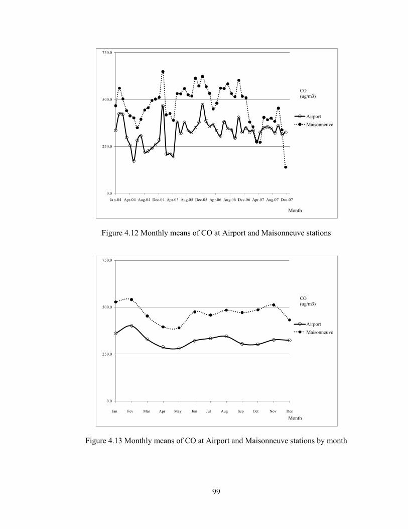
99
Figure 4.12 Monthly means of CO at Airport and Maisonneuve stations
Figure 4.13 Monthly means of CO at Airport and Maisonneuve stations by month
0.0
250.0
500.0
750.0
Jan-04 Apr-04 Aug-04 Dec-04 Apr-05 Aug-05 Dec-05 Apr-06 Aug-06 Dec-06 Apr-07 Aug-07 Dec-07
AirportMaisonneuve
Month
CO (ug/m3)
0.0
250.0
500.0
750.0
1 2 3 4 5 6 7 8 9 10 11 12
AirportMaisonneuve
Month
CO (ug/m3)
Jan Fev Mar Apr May Jun Jul Aug Sep Oct Nov Dec

100
Figure 4.14 Monthly means of SR at Airport station
Figure 4.15 Monthly means of SR at Airport station by month
0.0
250.0
500.0
750.0
1000.0
1250.0
Jan-04 Apr-04 Aug-04 Dec-04 Apr-05 Aug-05 Dec-05 Apr-06 Aug-06 Dec-06 Apr-07 Aug-07 Dec-07
Airport
Month
SR (W/m2)
0.0
250.0
500.0
750.0
1000.0
1250.0
1 2 3 4 5 6 7 8 9 10 11 12
Airport
Month
SR (W/m2)
Jan Fev Mar Apr May Jun Jul Aug Sep Oct Nov Dec

101
Figure 4.16 Monthly means of Temp at Airport station
Figure 4.17 Monthly means of Temp at Airport station by month
-25.0
-15.0
-5.0
5.0
15.0
25.0
Jan-04 Apr-04 Aug-04 Dec-04 Apr-05 Aug-05 Dec-05 Apr-06 Aug-06 Dec-06 Apr-07 Aug-07 Dec-07
Airport
Month
Temp (oC)
-25.0
-20.0
-15.0
-10.0
-5.0
0.0
5.0
10.0
15.0
20.0
25.0
1 2 3 4 5 6 7 8 9 10 11 12
Airport
Month
Temp (oC)
Jan Fev Mar Apr May Jun Jul Aug Sep Oct Nov Dec

102
Figure 4.18 Monthly means of DP at Airport station
Figure 4.19 Monthly means of DP at Airport station by month
-25.0
-15.0
-5.0
5.0
15.0
25.0
Jan-04 Apr-04 Aug-04 Dec-04 Apr-05 Aug-05 Dec-05 Apr-06 Aug-06 Dec-06 Apr-07 Aug-07 Dec-07
Airport
Month
DP(oC)
-25.0
-20.0
-15.0
-10.0
-5.0
0.0
5.0
10.0
15.0
20.0
25.0
1 2 3 4 5 6 7 8 9 10 11 12
Airport
Month
DP (oC)
Jan Fev Mar Apr May Jun Jul Aug Sep Oct Nov Dec

103
Figure 4.20 Monthly means of Press at Airport station
Figure 4.21 Monthly means of Press at Airport station by month
100.0
100.5
101.0
101.5
102.0
102.5
Jan-04 Apr-04 Aug-04 Dec-04 Apr-05 Aug-05 Dec-05 Apr-06 Aug-06 Dec-06 Apr-07 Aug-07 Dec-07
Airport
Month
Press (KPa)
100.0
100.5
101.0
101.5
102.0
102.5
1 2 3 4 5 6 7 8 9 10 11 12
Airport
Month
Press (KPa)
Jan Fev Mar Apr May Jun Jul Aug Sep Oct Nov Dec

104
Figure 4.22 Monthly means of Precip at Airport station
Figure 4.23 Monthly means of Precip at Airport and stations by month
0.0
0.1
0.2
0.3
0.4
Jan-04 Apr-04 Aug-04 Dec-04 Apr-05 Aug-05 Dec-05 Apr-06 Aug-06 Dec-06 Apr-07 Aug-07 Dec-07
Airport
Month
Precip (mm)
0.0
0.1
0.2
0.3
0.4
1 2 3 4 5 6 7 8 9 10 11 12
Airport
Month
Precip (mm)
Jan Fev Mar Apr May Jun Jul Aug Sep Oct Nov Dec

105
The wind direction is reported by RSQA as (NE, E, SE, S, SW, W, NW, N). We
transformed these values to (1, 2, 3, 4, 5, 6, 7, 8) respectively. The corresponding mean
values of the daily maximum 1-h ozone concentration between January 2004 and
December 2007 were plotted as a function of the transformed numerical values of wind
direction. Results are tabulated in Appendix G. Then, we followed the procedure
described in Chaloulakou et. al (2003) to derive the wind direction index (WDI). The
rationale of this procedure is to remove the discontinuity of the wind direction angle at
360o by fitting the following sinusoidal function:
𝑊𝐷𝐼 = 1 + sin (ψ−𝜃𝑤𝜋) (4.1)
where θw is the wind direction expressed in radians (with 0o corresponding to the North)
and ψ is an estimated parameter accounting for the phase shift.
The inclusion of wind speed and wind direction in this study does not violate the
assumption of non-stochasticity of input variablesfor the regression models. The pseudo-
randomness of WS and WDI is smoothed over the 1-hour averaging period of the data
collection. Both variables WS and WDI point out to the role, which is primarily of
physical transport of precursor species and mixing, that wind plays in the surface
boundary layer with respect to the formation of ozone and fine particulate matter.
The value of ψ has been determined to be -0.79 for both Airport and Maisonneuve
stations. From the definition of the index, it emerges that when the wind is southwesterly
(i.e. WD is 5), WDI is 2.0 (maximum value). Conversely, when the wind is northeasterly
(i.e. WD is 1), WDI is 0.0 (minimum value). These wind directions correspond to the
maximum and minimum values of the daily 1-h maximum O3, respectively.
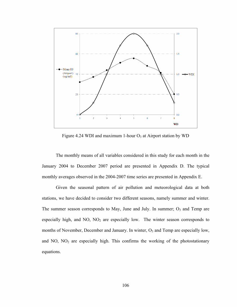
106
Figure 4.24 WDI and maximum 1-hour O3 at Airport station by WD
The monthly means of all variables considered in this study for each month in the
January 2004 to December 2007 period are presented in Appendix D. The typical
monthly averages observed in the 2004-2007 time series are presented in Appendix E.
Given the seasonal pattern of air pollution and meteorological data at both
stations, we have decided to consider two different seasons, namely summer and winter.
The summer season corresponds to May, June and July. In summer; O3 and Temp are
especially high, and NO, NO2 are especially low. The winter season corresponds to
months of November, December and January. In winter, O3 and Temp are especially low,
and NO, NO2 are especially high. This confirms the working of the photostationary
equations.
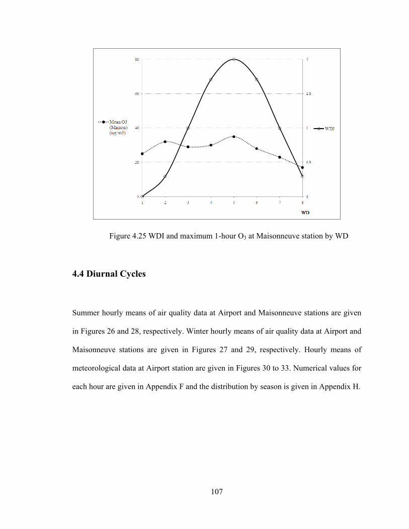
107
Figure 4.25 WDI and maximum 1-hour O3 at Maisonneuve station by WD
4.4 Diurnal Cycles
Summer hourly means of air quality data at Airport and Maisonneuve stations are given
in Figures 26 and 28, respectively. Winter hourly means of air quality data at Airport and
Maisonneuve stations are given in Figures 27 and 29, respectively. Hourly means of
meteorological data at Airport station are given in Figures 30 to 33. Numerical values for
each hour are given in Appendix F and the distribution by season is given in Appendix H.

108
Figure 4.26 Diurnal cycle of O3, PM2.5, NO, NO2 and CO (in μg/m3) at Airport station (Summer)
Figure 4.27 Diurnal cycle of O3, PM2.5, NO, NO2 and CO (in μg/m3) at Airport station (Winter)

109
Figure 4.28 Diurnal cycle of O3, PM2.5, NO, NO2 and CO (in μg/m3) at Maisonneuve
station (Summer)
Figure 4.29 Diurnal cycle of O3, PM2.5, NO, NO2 and CO (in μg/m3) at Maisonneuve
station (Winter)

110
Figure 4.30 Diurnal cycle of Temp and DP (oC); and Press (kPa) at Airport station
(Summer)
Figure 4.31 Diurnal cycle of Temp and DP (oC); and Press (kPa) at Airport station
(Winter)

111
Figure 4.32 Diurnal cycle of Precip (mm) and SR (W/m2) at Airport station (Summer)
Figure 4.33 Diurnal cycle of Precip (mm) and SR (W/m2) at Airport station (Winter)

112
On a typical early-morning in Montréal - that is between 05h00 and 07h00; NO,
NO2 and CO concentrations peak with increased vehicular traffic. At twilight, the
nitrogen dioxide photolysis (dissociation of nitrogen dioxide into nitric oxide and oxygen
radical) is limited due to low solar radiation (and temperature). At the same time, O3
concentrations decreases because i) ozone oxidises NO to NO2 and is converted back to
molecular oxygen, ii) solar radiation and temperature are still low limiting the amount of
free energy for NO2 dissociation, iii) to low VOC levels (given low VOC volatility), and
iii) limited photolysis of VOC allowing the alternate pathway of NO conversion to NO2.
After 07h00, with increased solar irradiation and temperature, NO and NO2
decrease and O3 concentrations increase. O3 increases because during the day light hours,
i) NO2 absorbs the energy of a photon light and dissociates into NO and an oxygen
radical, then the oxygen radical combines with O2 to form O3, and ii) because of the
increased VOC levels (higher volatility) which enables the oxidation process of
hydrocarbons by hydroxyl radical (OH•) offering another pathway which converts NO to
NO2.
We note that O3 peaks at 15h00. Then, in the afternoon, with decreasing solar
irradiation, ozone concentrations decrease to stabilize at 21h00 in summer and 17h00 in
winter. NO, NO2 and CO increases with vehicular traffic peak at 21h00 in summer and
18h00 in winter. At sunset, the NO2 dioxide photolysis is again limited due to low solar
irradiation. At these times of day, ozone and nitric oxide combine to yield nitrogen
dioxide and oxygen. The data confirms these important ozone formation mechanisms in
Montréal.
113
O3 levels in Maisonneuve are lower than at Airport. The data indicates that at
Airport, with lower NO and NO2 concentrations, NOx makes a net positive contribution
to photochemical ozone formation, but at Maisonneuve with higher concentrations,
typical of downtown Montréal, the balance is shifted to ozone consumption. The data
confirms that NOx scavenging occur in the city as higher NOx emissions locally decrease
ozone.
Given the diurnal pattern of air pollution and meteorological data at both stations,
we have decided consider two different periods in our study, namely day and night. The
day period corresponds to 11h00 to 16h00. The night period corresponds to 22h00 to
04h00.
Tables 4.3 to 4.6 show the correlation between variables for summer and winter
seasons by day and night periods. Correlation coefficients between pollutants and
meteorological variables were analysed to evaluate the influence of each variable on O3
and PM2.5 concentration. These coefficients provide a measure of the linear relation
between two variables and also indicate the existence of collinearity between the
explanatory variables.
At Airport station, summer ozone concentrations were correlated with PM2.5 and
temperature during day time; and with NO2 and wind speed during night time. Winter
ozone concentrations were negatively correlated with PM2.5, NO, NO2 and CO during
both day and night time. At Maisonneuve station, ozone concentrations were correlated
with NO during both day and night periods. During daylight hours, ozone was correlated
with temperature. Overall, the correlations of ozone with meteorological variables were
generally weak.

114
At Airport station, summer PM2.5 concentrations were correlated with O3, CO and
temperature during both day and night periods. Winter PM2.5 concentrations were
negatively correlated with PM2.5, NO, NO2 and CO during both day and night time. High
correlation was found between PM2.5 and O3, NO, NO2 at Maisonneuve during both
periods in winter. The correlations of PM2.5 with meteorological variables were generally
weak.
Cross correlation between precursor species were identified, such as NO and CO
(0.70), O3 and NO2 (-0.70) and NO and NO2 (0.65), demonstrating the existence of
collinearity between the variables. Also, the correlation between temperature and dew
point was positive and highly significant, as expected.

115
Table 4.3 Correlation of variables (Summer / Day)
Table 4.4 Correlation of variables (Summer / Night)
Summer/Day O3 (Airport) PM2.5 (Airport) O3 (Maison) PM2.5 (Maison)O3 (Airport) 1.00 0.51 0.90 0.49PM2.5 (Airport) 0.51 1.00 0.44 0.92NO (Airport) -0.34 0.09 -0.28 0.03NO2 (Airport) -0.16 0.31 -0.18 0.28CO (Airport) 0.10 0.62 0.08 0.60O3 (Maison) 0.90 0.44 1.00 0.39PM2.5 (Maison) 0.49 0.92 0.39 1.00NO (Maison) -0.55 -0.18 -0.71 -0.14NO2 (Maison) 0.32 0.37 0.01 0.46CO (Maison) -0.09 0.21 -0.30 0.27SR -0.05 0.01 0.04 0.00Temp 0.62 0.50 0.58 0.48DP 0.27 0.55 0.26 0.55Press 0.27 -0.05 0.30 -0.08Precip -0.20 -0.07 -0.22 -0.04WS -0.05 -0.13 -0.03 -0.15WDI 0.30 0.12 0.25 0.11
Summer/Night O3 (Airport) PM2.5 (Airport) O3 (Maison) PM2.5 (Maison)O3 (Airport) 1.00 0.12 0.85 0.21PM2.5 (Airport) 0.12 1.00 0.23 0.89NO (Airport) -0.35 0.09 -0.22 0.05NO2 (Airport) -0.54 0.34 -0.29 0.23CO (Airport) -0.22 0.61 -0.09 0.53O3 (Maison) 0.85 0.23 1.00 0.23PM2.5 (Maison) 0.21 0.89 0.23 1.00NO (Maison) -0.31 -0.03 -0.49 0.03NO2 (Maison) -0.22 0.33 -0.31 0.36CO (Maison) -0.04 0.09 -0.15 0.13SR -0.04 0.04 -0.07 0.06Temp 0.26 0.50 0.23 0.51DP 0.09 0.46 0.06 0.47Press -0.19 0.07 -0.07 0.02Precip 0.05 0.05 0.02 0.07WS 0.44 -0.28 0.31 -0.25WDI 0.37 0.06 0.26 0.12

116
Table 4.5 Correlation of variables (Winter / Day)
Table 4.6 Correlation of variables (Winter / Night)
Winter/Day O3 (Airport) PM2.5 (Airport) O3 (Maison) PM2.5 (Maison)O3 (Airport) 1.00 -0.54 0.80 -0.51PM2.5 (Airport) -0.54 1.00 -0.40 0.79NO (Airport) -0.48 0.74 -0.32 0.51NO2 (Airport) -0.74 0.74 -0.53 0.62CO (Airport) -0.64 0.79 -0.43 0.61O3 (Maison) 0.80 -0.40 1.00 -0.48PM2.5 (Maison) -0.51 0.79 -0.48 1.00NO (Maison) -0.43 0.43 -0.61 0.58NO2 (Maison) -0.26 0.42 -0.52 0.53CO (Maison) -0.53 0.48 -0.66 0.64SR -0.03 0.03 -0.07 0.06Temp -0.36 0.05 -0.41 0.09DP -0.51 0.14 -0.52 0.17Press 0.24 0.04 0.24 -0.01Precip -0.20 -0.03 -0.13 -0.04WS 0.31 -0.38 0.34 -0.39WDI 0.41 -0.32 0.13 -0.30
Winter/Night O3 (Airport) PM2.5 (Airport) O3 (Maison) PM2.5 (Maison)O3 (Airport) 1.00 -0.60 0.79 -0.52PM2.5 (Airport) -0.60 1.00 -0.53 0.74NO (Airport) -0.46 0.70 -0.39 0.41NO2 (Airport) -0.80 0.70 -0.56 0.55CO (Airport) -0.55 0.79 -0.43 0.49O3 (Maison) 0.79 -0.53 1.00 -0.59PM2.5 (Maison) -0.52 0.74 -0.59 1.00NO (Maison) -0.44 0.46 -0.56 0.60NO2 (Maison) -0.56 0.57 -0.69 0.61CO (Maison) -0.39 0.46 -0.52 0.57SR -0.03 -0.06 -0.02 -0.04Temp -0.13 -0.07 -0.24 0.00DP -0.21 -0.01 -0.30 0.06Press -0.11 0.19 -0.01 0.12Precip -0.03 -0.08 0.00 -0.07WS 0.60 -0.42 0.50 -0.34WDI 0.27 -0.19 0.08 -0.15

117
4.5 Dataset Preparation
Data from Airport station (O3, PM2.5, NO, NO2, CO, SR, Temp, Press, DP, Precip, WS
and WDI) and from Maisonneuve station (O3, PM2.5, NO, NO2 and CO) observed in
summer/winter seasons and in day/night periods at time t (present time) were set in a
matrix form. Then we added columns to indicate the observed values of O3 and PM2.5 at t
+ 1 (future time, 1-hour window). The 1-hour ahead values of O3 and PM2.5 were referred
to as OP and PP, respectively. Each variable carried a subscript “Airport” or “Maison” to
indicate its source.
We eliminated the rows of each pattern where there was at least one observation
missing, from either station. The resulting matrix contained 17 columns and
4,976 rows. At this point, we made an informed decision not to include a “production”
subset in order to simplify subsequent analysis. Then, we randomly selected rows in the
matrix for either learning or testing in such a way that the selection was uniformly
distributed. We applied a subroutine such that:
1. at least 50% (but no more than 55%) of the observations were tagged as
“learning”;
2. 50% of the top 50 observations for each variable were tagged “testing”;
3. 50% of the bottom 50 observations for each variable were tagged “testing”
The learning dataset was used for model training and the testing dataset was used for
model validation. All models were trained and validated using the same datasets. Table.

118
4.7 summarises the final split count of the main observation matrix into the learning and
testing datasets used for forecasting (Case Studies 1 through 4 inclusively).
Table 4.7 Learning and testing counts
The dataset used in Case Study 5 differed from the previous datasets as the
objective of this case study was to model daily means of ozone at Maisonneuve station
with inclusion of available VOC data. In addition to the set of air quality and
meteorological data used in the previous four case studies, the concentration values of
142 different VOC species that were available at six days interval were included. The
original dataset with no missing values contained 186 rows of observations. The same
subroutine was applied. The dataset was split into training and validation datasets
containing 102 and 84 observations, respectively.
Period Cases Learning TestingSummer
Day 1002 506 496Night 1224 629 595
WinterDay 1231 650 581Night 1519 796 723
Total 4976 2581 2395

119
Chapter 5
Results
In this section we present the result of four case studies. In Case Study 1, we investigate
O3 at Airport. In Case Study 2, we investigate PM2.5 at Airport. In Case Study 3, we
investigate O3 at Maisonneuve. In Case Study 4, we investigate PM2.5 at Maisonneuve.
For each case study we consider different model configuration for summer-day,
summer-night, winter-day and winter-night. The model outputs for Case Study 1 are
presented in Appendix I. Error diagnostics for Case Study 1 are presented in Appendix J.
5.1 Case Study 1: O3 Forecast at Airport Station
5.1.1 Summer
Different models to forecast 1-hour ahead O3 concentrations at Airport station during the
summer season were developed. We considered two distinct periods, namely day and
night-time. The developed models were based on MLR, PCR, MARS 1, MARS 2, ANN,
PC-ANN and PC*-ANN methods.

120
The observed means of the O3 responses were 78.9 and 37.0 μg/m3 during the day
and night-time respectively. The 75% percentile of O3 concentrations were 96 and 55
μg/m3 for the day and night-time period, in that order. The overall performance metrics
and the success forecasting rates at the 75% percentile concentrations obtained with the
learning dataset are shown in Table 5.1 (PCR and MARS 1), Table 5.2 (MLR, MARS 2
and ANN) and Table 5.3 (PC-ANN and PC*-ANN).
Model suitability was assessed considering the overall performance metrics and
the success forecasting rates at the 75% percentile concentrations obtained in the
validation phase. These results are shown in Table 5.4 (PCR and MARS 1), Table 5.5
(MLR, MARS 2 and ANN) and Table 5.6 (PC-ANN and PC*-ANN).
Closely studying day-time results, the following inferences have been made:
1. R2 ranged (0.48 – 0.68) with a corresponding r in the (0.69 – 0.82) range. In terms
of these two metrics, PC-ANN performed the best, closely followed by MARS 1.
2. MAPE ranged (14% – 15%). All models yielded values in the same order of
magnitude.
3. MBE ranged (-3.0 – -0.8), MAE ranged (13.0 – 15.5) and RMSE ranged (16.6 –
21.5). In terms of these three metrics, MARS 1 performed the best, closely
followed by PC-ANN and MARS 2.
4. TPR ranged (0.59 – 0.73), FPR ranged (0.07 – 0.12) and SI ranged (0.51 – 0.65).
In terms of these three metrics, MARS 1 performed the best, closely followed by
MARS 2 and PC-ANN.

121
Similarly, the following inferences have been made with respect to night-time
results:
1. R2 ranged (0.51 – 0.69) with a corresponding r in the (0.71 – 0.83) range. In terms
of these two metrics, ANN performed the best, closely followed by MARS 2 and
PC-ANN.
2. MAPE ranged (20% – 31%). In terms of this metric, MARS 2 performed the best
closely followed by PC-ANN.
3. MBE ranged (-0.9 – 0.3), MAE ranged (11.5 – 14.1) and RMSE ranged (15.2 –
18.9). In terms of these three metrics, ANN performed the best, closely followed
by MARS 2.
4. TPR ranged (0.46 – 0.67), FPR ranged (0.07 – 0.12) and SI ranged (0.39 – 0.59).
In terms of these three metrics, PC-ANN performed the best, closely followed by
MARS 2.
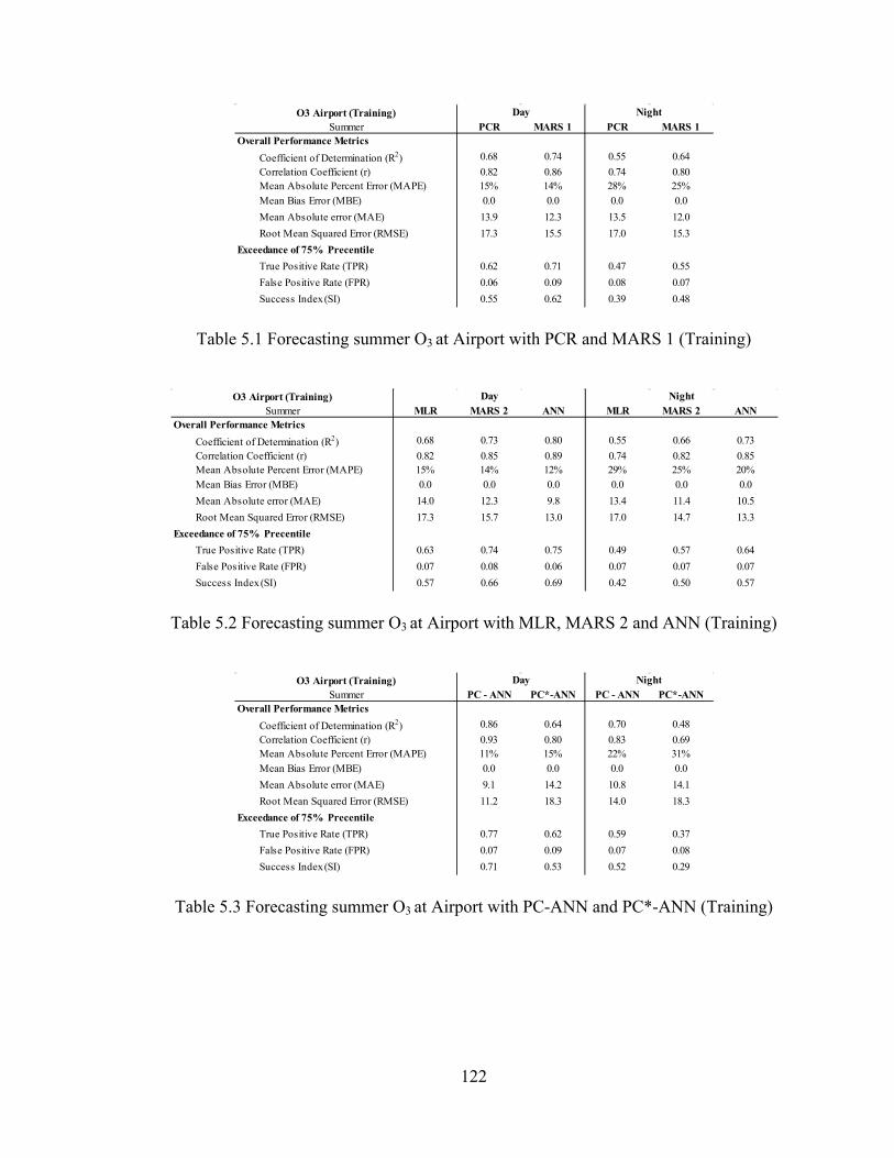
122
Table 5.1 Forecasting summer O3 at Airport with PCR and MARS 1 (Training)
Table 5.2 Forecasting summer O3 at Airport with MLR, MARS 2 and ANN (Training)
Table 5.3 Forecasting summer O3 at Airport with PC-ANN and PC*-ANN (Training)
O3 Airport (Training)Summer PCR MARS 1 PCR MARS 1
Overall Performance MetricsCoefficient of Determination (R2) 0.68 0.74 0.55 0.64Correlation Coefficient (r) 0.82 0.86 0.74 0.80Mean Absolute Percent Error (MAPE) 15% 14% 28% 25%Mean Bias Error (MBE) 0.0 0.0 0.0 0.0Mean Absolute error (MAE) 13.9 12.3 13.5 12.0Root Mean Squared Error (RMSE) 17.3 15.5 17.0 15.3
Exceedance of 75% PrecentileTrue Positive Rate (TPR) 0.62 0.71 0.47 0.55False Positive Rate (FPR) 0.06 0.09 0.08 0.07Success Index (SI) 0.55 0.62 0.39 0.48
Day Night
O3 Airport (Training)Summer MLR MARS 2 ANN MLR MARS 2 ANN
Overall Performance MetricsCoefficient of Determination (R2) 0.68 0.73 0.80 0.55 0.66 0.73Correlation Coefficient (r) 0.82 0.85 0.89 0.74 0.82 0.85Mean Absolute Percent Error (MAPE) 15% 14% 12% 29% 25% 20%Mean Bias Error (MBE) 0.0 0.0 0.0 0.0 0.0 0.0Mean Absolute error (MAE) 14.0 12.3 9.8 13.4 11.4 10.5Root Mean Squared Error (RMSE) 17.3 15.7 13.0 17.0 14.7 13.3
Exceedance of 75% PrecentileTrue Positive Rate (TPR) 0.63 0.74 0.75 0.49 0.57 0.64False Positive Rate (FPR) 0.07 0.08 0.06 0.07 0.07 0.07Success Index (SI) 0.57 0.66 0.69 0.42 0.50 0.57
Day Night
O3 Airport (Training)Summer PC - ANN PC*-ANN PC - ANN PC*-ANN
Overall Performance MetricsCoefficient of Determination (R2) 0.86 0.64 0.70 0.48Correlation Coefficient (r) 0.93 0.80 0.83 0.69Mean Absolute Percent Error (MAPE) 11% 15% 22% 31%Mean Bias Error (MBE) 0.0 0.0 0.0 0.0Mean Absolute error (MAE) 9.1 14.2 10.8 14.1Root Mean Squared Error (RMSE) 11.2 18.3 14.0 18.3
Exceedance of 75% PrecentileTrue Positive Rate (TPR) 0.77 0.62 0.59 0.37False Positive Rate (FPR) 0.07 0.09 0.07 0.08Success Index (SI) 0.71 0.53 0.52 0.29
Day Night

123
Table 5.4 Forecasting summer O3 at Airport with PCR and MARS 1 (Validation)
Table 5.5 Forecasting summer O3 at Airport with MLR, MARS 2 and ANN (Validation)
Table 5.6 Forecasting summer O3 at Airport with PC-ANN and PC*-ANN (Validation)
O3 Airport (Validation)Summer PCR MARS 1 PCR MARS 1
Overall Performance Metrics
Coefficient of Determination (R2) 0.48 0.68 0.60 0.65Correlation Coefficient (r) 0.69 0.82 0.78 0.81Mean Absolute Percent Error (MAPE) 14% 14% 25% 22%Mean Bias Error (MBE) -3.0 -1.3 -0.6 0.3Mean Absolute error (MAE) 15.5 13.0 13.2 12.3Root Mean Squared Error (RMSE) 21.5 16.6 17.0 16.0
Exceedance of 75% PrecentileTrue Positive Rate (TPR) 0.62 0.72 0.54 0.59False Positive Rate (FPR) 0.08 0.07 0.08 0.07Success Index (SI) 0.54 0.65 0.46 0.52
Day Night
O3 Airport (Validation)Summer MLR MARS 2 ANN MLR MARS 2 ANN
Overall Performance Metrics
Coefficient of Determination (R2) 0.48 0.66 0.58 0.60 0.68 0.69Correlation Coefficient (r) 0.69 0.81 0.76 0.77 0.83 0.83Mean Absolute Percent Error (MAPE) 14% 14% 15% 25% 20% 21%Mean Bias Error (MBE) -2.5 -1.3 -1.7 -0.6 -0.2 -0.1Mean Absolute error (MAE) 15.4 13.2 13.1 13.2 11.5 11.8Root Mean Squared Error (RMSE) 21.5 17.2 18.9 17.2 15.2 15.2
Exceedance of 75% PrecentileTrue Positive Rate (TPR) 0.59 0.73 0.65 0.53 0.63 0.65False Positive Rate (FPR) 0.08 0.10 0.09 0.08 0.08 0.12Success Index (SI) 0.51 0.63 0.54 0.45 0.55 0.53
Day Night
O3 Airport (Validation)Summer PC - ANN PC*-ANN PC - ANN PC*-ANN
Overall Performance Metrics
Coefficient of Determination (R2) 0.68 0.56 0.68 0.51Correlation Coefficient (r) 0.83 0.75 0.83 0.71Mean Absolute Percent Error (MAPE) 15% 15% 21% 31%Mean Bias Error (MBE) -0.8 -1.8 -0.9 0.0Mean Absolute error (MAE) 13.3 15.0 11.8 14.1Root Mean Squared Error (RMSE) 16.9 19.5 15.3 18.9
Exceedance of 75% PrecentileTrue Positive Rate (TPR) 0.72 0.66 0.67 0.46False Positive Rate (FPR) 0.09 0.12 0.08 0.07Success Index (SI) 0.63 0.54 0.59 0.39
Day Night
124
These results indicate that i) the performance of PCR is not significantly better
than the performance of MLR, ii) MARS 2 marginally outperforms MARS 1, iii) PC-
ANN marginally outperforms ANN, iv) while successfully achieving reduction in the
dimensionality of the input vector, PC*-ANN is outperformed by ANN. Therefore, we
have opted to focus our attention on MLR, MARS 2 and ANN models for subsequent
analysis related to ozone.

125
5.1.2 Winter
MLR, MARS 2 and ANN models were developed to forecast 1-hour ahead O3
concentrations at Airport station during the winter season. We considered two distinct
periods, namely day and night-time.
The observed means of the O3 responses were 36.9 and 29.5 μg/m3 during the day
and night-time respectively. The 75% percentile of O3 concentrations were 55 and 44
μg/m3 for the day and night-time period, in that order. The overall performance metrics
and the success forecasting rates at the 75% percentile concentrations obtained with the
learning dataset are shown in Table 5.7.
Model suitability was assessed considering the overall performance metrics and
the success forecasting rates at the 75% percentile concentrations obtained in the
validation phase. These results are shown in Table 5.8.
Closely studying day-time results, the following inferences have been made:
1. R2 ranged (0.70 – 0.78) with a corresponding r in the (0.84 – 0.88) range. In terms
of these two metrics, MARS 2 performed the best.
2. MAPE ranged (11% – 16%). In terms of this metric, MARS 2 performed the best.
3. MBE ranged (-3.0 – -0.5), MAE ranged (7.1 – 8.3) and RMSE ranged (9.1 –
10.7). In terms of these three metrics, MARS 2 performed the best.
4. TPR ranged (0.43 – 0.66), FPR ranged (0.05 – 0.07) and SI ranged (0.39 – 0.59).
In terms of these three metrics, ANN performed the best.

126
Similarly, the following inferences have been made with respect to night-time
results:
1. R2 ranged (0.73 – 0.77) with a corresponding r in the (0.85 – 0.88) range. In terms
of these two metrics, ANN model performed the best.
2. MAPE ranged (14% – 17%). In terms of this metric, MARS 2 performed the best.
3. MBE ranged (-0.5 – 0.6), MAE ranged (7.0 – 7.9) and RMSE ranged (9.1 –
10.1). In terms of these three metrics, ANN performed the best.
4. TPR ranged (0.65 – 0.75), FPR ranged (0.08 – 0.09) and SI ranged (0.57 – 0.65).
In terms of these three metrics, ANN performed the best.

127
Table 5.7 Forecasting winter O3 at Airport with MLR, MARS 2 and ANN (Training)
Table 5.8 Forecasting winter O3 at Airport with MLR, MARS 2 and ANN (Validation)
O3 Airport (Training)Winter MLR MARS 2 ANN MLR MARS 2 ANN
Overall Performance MetricsCoefficient of Determination (R2) 0.73 0.81 0.82 0.74 0.80 0.82Correlation Coefficient (r) 0.85 0.90 0.91 0.86 0.89 0.90Mean Absolute Percent Error (MAPE) 13% 9% 9% 15% 12% 12%Mean Bias Error (MBE) 0.0 0.0 0.0 0.0 0.0 0.0Mean Absolute error (MAE) 7.9 6.7 6.6 7.7 6.6 6.3Root Mean Squared Error (RMSE) 10.4 8.7 8.4 9.6 8.5 8.0
Exceedance of 75% PrecentileTrue Positive Rate (TPR) 0.54 0.74 0.78 0.62 0.72 0.76False Positive Rate (FPR) 0.04 0.06 0.07 0.04 0.04 0.07Success Index (SI) 0.49 0.68 0.71 0.58 0.68 0.69
NightDay
O3 Airport (Validation)Winter MLR MARS 2 ANN MLR MARS 2 ANN
Overall Performance Metrics
Coefficient of Determination (R2) 0.70 0.78 0.77 0.73 0.76 0.77Correlation Coefficient (r) 0.84 0.88 0.88 0.85 0.87 0.88Mean Absolute Percent Error (MAPE) 16% 11% 11% 17% 14% 15%Mean Bias Error (MBE) 0.5 -0.3 -0.3 -0.6 -0.5 -0.6Mean Absolute error (MAE) 8.3 7.1 7.2 7.9 7.3 7.0Root Mean Squared Error (RMSE) 10.7 9.1 9.3 10.1 9.4 9.1
Exceedance of 75% PrecentileTrue Positive Rate (TPR) 0.43 0.63 0.66 0.65 0.69 0.75False Positive Rate (FPR) 0.05 0.06 0.07 0.08 0.09 0.09Success Index (SI) 0.39 0.56 0.59 0.57 0.60 0.65
Day Night

128
5.2 Case Study 2: PM2.5 Forecast at Airport Station
5.2.1 Summer
Different models to forecast 1-hour ahead PM2.5 concentrations at Airport station during
the summer season were developed. We considered two distinct periods, namely day and
night-time. The developed models were based on MLR, PCR, MARS 1, MARS 2, ANN,
PC-ANN and PC*-ANN methods.
The observed means of the PM2.5 responses were 10.7 and 8.2 μg/m3 during the
day and night-time respectively. The 75% percentile of PM2.5 concentrations were 11 and
12 μg/m3 for the day and night-time period, in that order. The overall performance
metrics and the success forecasting rates at the 75% percentile concentrations obtained
with the learning dataset are shown in Table 5.9 (PCR and MARS 1), Table 5.10 (MLR,
MARS 2 and ANN) and Table 5.11 (PC-ANN and PC*-ANN).
Model suitability was assessed considering the overall performance metrics and
the success forecasting rates at the 75% percentile concentrations obtained in the
validation phase. These results are shown in Table 5.12 (PCR and MARS 1), Table 5.13
(MLR, MARS 2 and ANN) and Table 5.14 (PC-ANN and PC*-ANN).
Closely studying day-time results, the following inferences have been made:
1. R2 ranged (0.48 – 0.74) with a corresponding r in the (0.69 – 0.86) range. In terms
of these two metrics, PC-ANN performed the best.

129
2. MAPE ranged (44% – 67%). In terms of this metrics, MARS 2 performed the
best.
3. MBE ranged (-3.0 – 0.5), MAE ranged (3.1 – 4.0) and RMSE ranged (4.9 – 6.7).
In terms of these three metrics, PC-ANN performed the best, closely followed by
MARS 2.
4. TPR ranged (0.77 – 0.88), FPR ranged (0.06 – 0.13) and SI ranged (0.70 – 0.75).
In terms of these three metrics, MARS 2 performed the best, closely followed by
ANN.
Similarly, the following inferences have been made with respect to night-time
results:
1. R2 ranged (0.47 – 0.57) with a corresponding r in the (0.68 – 0.75) range. In terms
of these two metrics, ANN model performed the best, closely followed by MARS
2.
2. MAPE ranged (47% – 56%). In terms of this metric, ANN performed the best.
3. MBE ranged (-0.2 – 0.1), MAE ranged (3.7 – 4.0) and RMSE ranged (5.6 – 6.5).
In terms of these three metrics, ANN performed the best, closely followed by
MARS 1.
4. TPR ranged (0.73 – 0.86), FPR ranged (0.08 – 0.16) and SI ranged (0.64 – 0.70).
In terms of these three metrics, ANN performed the best, closely followed by
MARS 2.

130
These results indicate that i) the performance of PCR is not significantly better
than the performance of MLR, ii) MARS 2 marginally outperforms MARS 1, iii) PC-
ANN marginally outperforms ANN, iv) while successfully achieving reduction in the
dimensionality of the input vector, PC*-ANN is outperformed by ANN. Therefore, we
have opted to focus our attention on MLR, MARS 2 and ANN models for subsequent
analysis related to particulate matter.

131
Table 5.9 Forecasting summer PM2.5 at Airport with PCR and MARS 1 (Training)
Table 5.10 Forecasting summer PM2.5 at Airport with MLR, MARS 2 and ANN (Training)
Table 5.11 Forecasting summer PM2.5 at Airport with PC-ANN and PC*-ANN (Training)
PM2.5 Airport (Training)Summer PCR MARS 1 PCR MARS 1
Overall Performance MetricsCoefficient of Determination (R2) 0.66 0.77 0.51 0.57Correlation Coefficient (r) 0.81 0.88 0.71 0.75Mean Absolute Percent Error (MAPE) 60% 39% 60% 51%Mean Bias Error (MBE) 0.0 0.0 0.0 0.0Mean Absolute error (MAE) 3.7 2.8 4.3 3.8Root Mean Squared Error (RMSE) 5.0 4.1 6.1 5.8
Exceedance of 75% PrecentileTrue Positive Rate (TPR) 0.90 0.91 0.85 0.76False Positive Rate (FPR) 0.14 0.08 0.18 0.14Success Index (SI) 0.77 0.83 0.67 0.62
Day Night
PM2.5 Airport (Training)Summer MLR MARS 2 ANN MLR MARS 2 ANN
Overall Performance MetricsCoefficient of Determination (R2) 0.66 0.84 0.84 0.51 0.60 0.56Correlation Coefficient (r) 0.81 0.92 0.91 0.71 0.78 0.75Mean Absolute Percent Error (MAPE) 59% 35% 36% 59% 50% 48%Mean Bias Error (MBE) 0.0 0.0 0.0 0.0 0.0 0.0Mean Absolute error (MAE) 3.7 2.4 2.5 4.2 3.8 3.9Root Mean Squared Error (RMSE) 5.0 3.4 3.5 6.1 5.5 5.8
Exceedance of 75% PrecentileTrue Positive Rate (TPR) 0.90 0.90 0.90 0.83 0.73 0.73False Positive Rate (FPR) 0.14 0.05 0.06 0.15 0.09 0.12Success Index (SI) 0.77 0.84 0.84 0.69 0.64 0.61
Day Night
PM2.5 Airport (Training)Summer PC - ANN PC*-ANN PC - ANN PC*-ANN
Overall Performance MetricsCoefficient of Determination (R2) 0.88 0.73 0.60 0.50Correlation Coefficient (r) 0.94 0.85 0.77 0.70Mean Absolute Percent Error (MAPE) 33% 43% 45% 49%Mean Bias Error (MBE) 0.0 0.0 -0.2 0.0Mean Absolute error (MAE) 2.2 3.0 3.6 4.1Root Mean Squared Error (RMSE) 3.0 4.4 5.6 6.2
Exceedance of 75% PrecentileTrue Positive Rate (TPR) 0.91 0.87 0.75 0.72False Positive Rate (FPR) 0.05 0.06 0.12 0.16Success Index (SI) 0.86 0.80 0.63 0.56
Day Night

132
Table 5.12 Forecasting summer PM2.5 at Airport with PCR and MARS 1 (Validation)
Table 5.13 Forecasting summer PM2.5 at Airport with MLR, MARS 2 and ANN
(Validation)
Table 5.14 Forecasting summer PM2.5 at Airport with PC-ANN and PC*-ANN
(Validation)
PM2.5 Airport (Validation)Summer PCR MARS 1 PCR MARS 1
Overall Performance Metrics
Coefficient of Determination (R2) 0.48 0.48 0.54 0.55Correlation Coefficient (r) 0.69 0.69 0.74 0.74Mean Absolute Percent Error (MAPE) 67% 46% 56% 52%Mean Bias Error (MBE) 0.3 0.5 0.1 -0.1Mean Absolute error (MAE) 4.0 3.4 4.0 3.9Root Mean Squared Error (RMSE) 6.7 6.7 5.7 5.7
Exceedance of 75% PrecentileTrue Positive Rate (TPR) 0.88 0.80 0.86 0.77False Positive Rate (FPR) 0.13 0.08 0.16 0.14Success Index (SI) 0.75 0.72 0.70 0.63
Day Night
PM2.5 Airport (Validation)Summer MLR MARS 2 ANN MLR MARS 2 ANN
Overall Performance Metrics
Coefficient of Determination (R2) 0.48 0.63 0.55 0.54 0.54 0.57Correlation Coefficient (r) 0.69 0.79 0.74 0.74 0.74 0.75Mean Absolute Percent Error (MAPE) 67% 44% 45% 56% 51% 47%Mean Bias Error (MBE) 0.3 0.3 -0.2 0.1 0.0 0.0Mean Absolute error (MAE) 4.0 3.2 3.3 3.9 3.9 3.7Root Mean Squared Error (RMSE) 6.7 5.7 6.6 5.7 5.8 5.6
Exceedance of 75% PrecentileTrue Positive Rate (TPR) 0.88 0.83 0.81 0.82 0.75 0.73False Positive Rate (FPR) 0.13 0.08 0.06 0.13 0.10 0.08Success Index (SI) 0.75 0.75 0.75 0.69 0.64 0.65
Day Night
PM2.5 Airport (Validation)Summer PC - ANN PC*-ANN PC - ANN PC*-ANN
Overall Performance Metrics
Coefficient of Determination (R2) 0.74 0.48 0.47 0.51Correlation Coefficient (r) 0.86 0.69 0.69 0.71Mean Absolute Percent Error (MAPE) 47% 51% 50% 50%Mean Bias Error (MBE) -0.3 0.0 -0.2 -0.1Mean Absolute error (MAE) 3.1 3.7 4.0 4.0Root Mean Squared Error (RMSE) 4.9 6.7 6.5 6.0
Exceedance of 75% PrecentileTrue Positive Rate (TPR) 0.83 0.77 0.76 0.74False Positive Rate (FPR) 0.08 0.07 0.09 0.15Success Index (SI) 0.75 0.70 0.67 0.59
Day Night

133
5.2.2 Winter
MLR, MARS 2 and ANN models were developed to forecast 1-hour ahead PM2.5
concentrations at Airport station during the winter season. We considered two distinct
scenarios, namely day and night-time.
The observed means of the PM2.5 responses were 8.3 and 5.5 μg/m3 during the
day and night-time respectively. The 75% percentile of PM2.5 concentrations were 8.0
and 10.0 μg/m3 for the day and night-time period, in that order. The overall performance
metrics and the success forecasting rates at the 75% percentile concentrations obtained
with the learning dataset are shown in Table 5.15.
Model suitability was assessed considering the overall performance metrics and
the success forecasting rates at the 75% percentile concentrations obtained in the
validation phase. These results are shown in Table 5.16.
Closely studying day-time results, the following inferences have been made:
1. R2 ranged (0.64 – 0.71) with a corresponding r in the (0.80 – 0.84) range. In terms
of these two metrics, ANN performed the best.
2. MAPE ranged (44% – 50%). In terms of this metric, MARS 2 performed the best.
3. All models averaged 0.1 for MBE, MAE ranged (2.8 – 3.1) and RMSE ranged
(3.9 – 4.4). In terms of these three metrics, ANN performed the best.
4. TPR ranged (0.67 – 0.75), FPR ranged (0.10 – 0.14) and SI ranged (0.54 – 0.65).
In terms of these three metrics, ANN performed the best.

134
Similarly, the following inferences have been made with respect to night-time
results:
1. R2 ranged (0.66 – 0.68) with a corresponding r in the (0.81 – 0.83) range. In terms
of these two metrics, MARS 2 model performed the best.
2. MAPE ranged (46% – 50%). In terms of this metric, MARS 2 performed the best.
3. MBE ranged (0.0 – 0.2), MAE ranged (3.0 – 3.3) and RMSE ranged (4.3 – 4.5).
In terms of these three metrics, MARS 2 performed the best.
4. TPR ranged (0.75 – 0.78), FPR ranged (0.10 – 0.11) and SI ranged (0.65 – 0.68).
In terms of these three metrics, MARS 2 performed the best.

135
Table 5.15 Forecasting winter PM2.5 at Airport with MLR, MARS 2 and ANN (Training)
Table 5.16 Forecasting winter PM2.5 at Airport with MLR, MARS 2 and ANN (Validation)
PM2.5 Airport (Training)Winter MLR MARS 2 ANN MLR MARS 2 ANN
Overall Performance MetricsCoefficient of Determination (R2) 0.68 0.74 0.76 0.62 0.70 0.64Correlation Coefficient (r) 0.82 0.86 0.87 0.79 0.84 0.80Mean Absolute Percent Error (MAPE) 45% 38% 41% 53% 46% 47%Mean Bias Error (MBE) 0.0 0.0 0.0 0.0 0.0 0.0Mean Absolute error (MAE) 2.9 2.6 2.5 3.1 2.8 3.0Root Mean Squared Error (RMSE) 4.3 3.9 3.8 4.3 3.8 4.2
Exceedance of 75% PrecentileTrue Positive Rate (TPR) 0.74 0.69 0.75 0.75 0.77 0.71False Positive Rate (FPR) 0.13 0.09 0.10 0.11 0.10 0.10Success Index (SI) 0.60 0.60 0.65 0.64 0.67 0.62
NightDay
PM2.5 Airport (Validation)Winter MLR MARS 2 ANN MLR MARS 2 ANN
Overall Performance Metrics
Coefficient of Determination (R2) 0.64 0.70 0.71 0.66 0.68 0.67Correlation Coefficient (r) 0.80 0.83 0.84 0.81 0.83 0.82Mean Absolute Percent Error (MAPE) 50% 44% 45% 53% 46% 47%Mean Bias Error (MBE) 0.1 0.1 0.1 0.1 0.2 0.0Mean Absolute error (MAE) 3.1 2.9 2.8 3.3 3.0 3.1Root Mean Squared Error (RMSE) 4.4 4.0 3.9 4.5 4.3 4.4
Exceedance of 75% PrecentileTrue Positive Rate (TPR) 0.69 0.67 0.75 0.77 0.78 0.75False Positive Rate (FPR) 0.14 0.13 0.10 0.11 0.10 0.10Success Index (SI) 0.55 0.54 0.65 0.66 0.68 0.65
Day Night

136
5.3 Case Study 3: O3 Forecast at Maisonneuve Station
5.3.1 Summer
Different models to forecast 1-hour ahead O3 concentrations at Maisonneuve station
during the summer season were developed. We considered two distinct scenarios, namely
day and night-time. The developed models were based on MLR, MARS 2 and ANN.
The observed means of the O3 responses were 49.5 and 31.1 μg/m3 during the day
and night-time respectively. The 75% percentile of O3 concentrations were 65 and 44
μg/m3 for the day and night-time period, in that order. The overall performance metrics
and the success forecasting rates at the 75% percentile concentrations obtained with the
learning dataset are shown in Table 5.17.
Model suitability was assessed considering the overall performance metrics and
the success forecasting rates at the 75% percentile concentrations obtained in the
validation phase. These results are shown in Table 5.18.
Closely studying day-time results, the following inferences have been made:
1. R2 ranged (0.61 – 0.70) with a corresponding r in the (0.78 – 0.84) range. In terms
of these two metrics, MARS 2 performed the best.
2. MAPE ranged (24% – 30%). In terms of these two metrics, MARS 2 performed
the best.
3. MBE ranged (0.3 – 0.7), MAE ranged (10.0 – 11.6) and RMSE ranged (12.9 –
14.8). In terms of these three metrics, MARS 2 performed the best.

137
4. TPR ranged (0.50 – 0.62), FPR ranged (0.07 – 0.10) and SI ranged (0.41 – 0.56).
In terms of these three metrics, MARS 2 performed the best.
Similarly, the following inferences have been made with respect to night-time
results:
1. R2 ranged (0.48 – 0.65) with a corresponding r in the (0.70 – 0.80) range. In terms
of these two metrics, ANN performed the best.
2. MAPE ranged (36% – 42%). In terms of this metric, ANN performed the best.
3. MBE ranged (-0.6 – -0.3), MAE ranged (9.8 – 11.8) and RMSE ranged (12.5 –
15.1). In terms of these three metrics, MARS 2 performed the best.
4. TPR ranged (0.47 – 0.57), FPR ranged (0.05 – 0.07) and SI ranged (0.41 – 0.50).
In terms of these three metrics, MARS 2 performed the best.

138
Table 5.17 Forecasting summer O3 at Maisonneuve with MLR, MARS 2 and ANN (Training)
Table 5.18 Forecasting summer O3 at Maisonneuve with MLR, MARS 2 and ANN
(Validation)
O3 Maisonneuve (Training)Summer MLR MARS 2 ANN MLR MARS 2 ANN
Overall Performance MetricsCoefficient of Determination (R2) 0.61 0.73 0.64 0.44 0.62 0.68Correlation Coefficient (r) 0.78 0.85 0.80 0.66 0.79 0.83Mean Absolute Percent Error (MAPE) 30% 24% 28% 39% 32% 30%Mean Bias Error (MBE) 0.0 0.0 0.0 0.0 0.0 0.0Mean Absolute error (MAE) 11.6 9.9 11.1 11.7 9.5 8.7Root Mean Squared Error (RMSE) 15.2 12.7 14.6 15.0 12.3 11.2
Exceedance of 75% PrecentileTrue Positive Rate (TPR) 0.55 0.64 0.63 0.43 0.57 0.58False Positive Rate (FPR) 0.08 0.08 0.11 0.09 0.07 0.05Success Index (SI) 0.47 0.56 0.52 0.35 0.50 0.53
Day Night
O3 Maisonneuve (Validation)Summer MLR MARS 2 ANN MLR MARS 2 ANN
Overall Performance Metrics
Coefficient of Determination (R2) 0.61 0.70 0.65 0.48 0.65 0.63Correlation Coefficient (r) 0.78 0.84 0.81 70% 80% 80%Mean Absolute Percent Error (MAPE) 29% 24% 26% 0.4 0.4 0.4Mean Bias Error (MBE) 0.3 0.4 0.7 -0.3 -0.3 -0.6Mean Absolute error (MAE) 11.6 10.0 11.0 11.8 9.8 10.2Root Mean Squared Error (RMSE) 14.8 12.9 14.0 15.1 12.5 13.0
Exceedance of 75% PrecentileTrue Positive Rate (TPR) 0.50 0.62 0.62 0.47 0.57 0.53False Positive Rate (FPR) 0.09 0.07 0.10 0.07 0.07 0.05Success Index (SI) 0.41 0.56 0.53 0.41 0.50 0.48
Day Night

139
5.3.2 Winter
MLR, MARS 2 and ANN models were developed to forecast 1-hour ahead O3
concentrations at Maisonneuve station during the winter season. We considered two
distinct scenarios, namely day and night-time.
The observed means of the O3 responses were 17.4 and 21.1 μg/m3 during the day
and night-time respectively. The 75% percentile of O3 concentrations were 27.0 and 31.0
μg/m3 for the day and night-time period, in that order. The overall performance metrics
and the success forecasting rates at the 75% percentile concentrations obtained with the
learning dataset are shown in Table 5.19.
Model suitability was assessed considering the overall performance metrics and
the success forecasting rates at the 75% percentile concentrations obtained in the
validation phase. These results are shown in Table 5.20.
Closely studying day-time results, the following inferences have been made:
1. R2 ranged (0.58 – 0.68) with a corresponding r in the (0.76 – 0.82) range. In
terms of these two metrics, ANN performed the best.
2. MAPE ranged (25% – 29%). In terms of this metric, MARS 2 performed the best.
3. MBE ranged (-0.1 – 0.3), MAE ranged (4.7 – 5.6) and RMSE ranged (6.4 – 6.5).
In terms of these three metrics, MARS 2 performed the best.
4. TPR ranged (0.53 – 0.67), FPR ranged (0.05 – 0.06) and SI ranged (0.47 – 0.61).
In terms of these three metrics, MARS 2 performed the best.

140
Similarly, the following inferences have been made with respect to night-time
results:
1. R2 ranged (0.63 – 0.71) with a corresponding r in the (0.80 – 0.84) range. In terms
of these two metrics, MARS 2 model performed the best.
2. MAPE ranged (25% – 28%). In terms of this metric, MARS 2 performed the best.
3. MBE ranged (-0.9 – 0.8), MAE ranged (5.4 – 6.1) and RMSE ranged (7.1 – 7.9).
In terms of these three metrics, MARS 2 performed the best.
4. TPR ranged (0.61 – 0.67), FPR ranged (0.05 – 0.09) and SI ranged (0.55 – 0.60).
In terms of these three metrics, MARS 2 performed the best.

141
Table 5.19 Forecasting winter O3 at Maisonneuve with MLR, MARS 2 and ANN
(Training)
Table 5.20 Forecasting winter O3 at Maisonneuve with MLR, MARS 2 and ANN
(Validation)
O3 Maisonneuve (Training)Winter MLR MARS 2 ANN MLR MARS 2 ANN
Overall Performance MetricsCoefficient of Determination (R2) 0.67 0.80 0.83 0.65 0.72 0.75Correlation Coefficient (r) 0.82 0.89 0.91 0.81 0.85 0.87Mean Absolute Percent Error (MAPE) 26% 23% 22% 27% 26% 25%Mean Bias Error (MBE) 0.0 0.0 0.0 0.0 0.0 0.0Mean Absolute error (MAE) 5.2 4.2 3.9 5.9 5.3 4.9Root Mean Squared Error (RMSE) 6.8 5.3 4.9 7.4 6.7 6.3
Exceedance of 75% PrecentileTrue Positive Rate (TPR) 0.68 0.77 0.78 0.58 0.68 0.69False Positive Rate (FPR) 0.04 0.04 0.04 0.05 0.05 0.07Success Index (SI) 0.65 0.73 0.75 0.53 0.63 0.62
NightDay
O3 Maisonneuve (Validation)Winter MLR MARS 2 ANN MLR MARS 2 ANN
Overall Performance Metrics
Coefficient of Determination (R2) 0.58 0.67 0.68 0.63 0.71 0.71Correlation Coefficient (r) 0.76 0.82 0.82 0.80 0.84 0.84Mean Absolute Percent Error (MAPE) 29% 25% 27% 28% 25% 26%Mean Bias Error (MBE) 0.3 0.0 -0.1 -0.9 -0.8 -0.8Mean Absolute error (MAE) 5.6 4.7 4.9 6.1 5.5 5.4Root Mean Squared Error (RMSE) 7.3 6.5 6.4 7.9 7.1 7.1
Exceedance of 75% PrecentileTrue Positive Rate (TPR) 0.53 0.67 0.64 0.61 0.67 0.66False Positive Rate (FPR) 0.05 0.06 0.06 0.05 0.07 0.09Success Index (SI) 0.47 0.61 0.58 0.55 0.60 0.57
Day Night

142
5.4 Case Study 4: PM2.5 Forecast at Maisonneuve
5.4.1 Summer
Different models to forecast 1-hour ahead PM2.5 concentrations at Maisonneuve station
during the summer season were developed. We considered two distinct scenarios, namely
day and night-time. The developed models were based on MLR, MARS 2 and ANN.
The observed means of the PM2.5 responses were 8.6 and 9.2 μg/m3 during the
day and night-time respectively. The 75% percentile of PM2.5 concentrations were 13 and
11 μg/m3 for the day and night-time period, in that order. The overall performance
metrics and the success forecasting rates at the 75% percentile concentrations obtained
with the learning dataset are shown in Table 5.21.
Model suitability was assessed considering the overall performance metrics and
the success forecasting rates at the 75% percentile concentrations obtained in the
validation phase. These results are shown in Table 5.22.
Closely studying day-time results, the following inferences have been made:
1. R2 ranged (0.44 – 0.47) with a corresponding r in the (0.66 – 0.68) range. In terms
of these two metrics, MARS 2 performed the best.
2. MAPE ranged (48% – 58%). In terms of this metrics, MARS 2 performed the
best.
3. MBE ranged (-0.1 – 0.2), MAE ranged (4.0 – 4.4) and RMSE ranged (6.7 – 6.9).
In terms of these three metrics, MARS 2 performed the best.

143
4. TPR ranged (0.69 – 0.82), FPR ranged (0.11 – 0.15) and SI ranged (0.58 – 0.67).
In terms of these three metrics, ANN performed the best.
Similarly, the following inferences have been made with respect to night-time
results:
1. R2 ranged (0.44 – 0.53) with a corresponding r in the (0.66– 0.73) range. In terms
of these two metrics, MARS 2 model performed the best.
2. MAPE ranged (48% – 57%). In terms of this metric, ANN performed the best.
3. MBE ranged (-0.1 – 0.1), MAE ranged (3.6 – 3.9) and RMSE ranged (5.2 – 5.7).
In terms of these three metrics, MARS 2 performed the best.
4. TPR ranged (0.71 – 0.74), FPR ranged (0.11 – 0.16) and SI ranged (0.56 – 0.62).
In terms of these three metrics, MARS 2 performed the best.

144
Table 5.21 Forecasting summer PM2.5 at Maisonneuve with MLR, MARS 2 and ANN
(Training)
Table 5.22 Forecasting summer PM2.5 at Maisonneuve with MLR, MARS 2 and ANN
(Validation)
PM2.5 Maisonneuve (Training)Summer MLR MARS ANN MLR MARS ANN
Overall Performance MetricsCoefficient of Determination (R2) 0.61 0.72 0.67 0.41 0.56 0.51Correlation Coefficient (r) 0.78 0.85 0.82 0.64 0.75 0.72Mean Absolute Percent Error (MAPE) 57% 44% 46% 61% 54% 50%Mean Bias Error (MBE) 0.0 0.0 0.0 0.0 0.0 0.0Mean Absolute error (MAE) 4.2 3.5 3.7 4.0 3.4 3.7Root Mean Squared Error (RMSE) 5.8 4.9 5.3 5.9 5.1 5.4
Exceedance of 75% PrecentileTrue Positive Rate (TPR) 0.83 0.76 0.74 0.75 0.75 0.72False Positive Rate (FPR) 0.13 0.07 0.08 0.16 0.11 0.13Success Index (SI) 0.70 0.68 0.66 0.59 0.64 0.59
Day Night
PM2.5 Maisonneuve (Validation)Summer MLR MARS ANN MLR MARS ANN
Overall Performance Metrics
Coefficient of Determination (R2) 0.44 0.47 0.46 0.44 0.53 0.48Correlation Coefficient (r) 0.66 0.68 0.68 0.66 0.73 0.69Mean Absolute Percent Error (MAPE) 58% 48% 48% 57% 56% 48%Mean Bias Error (MBE) -0.1 0.2 0.0 0.0 -0.1 0.1Mean Absolute error (MAE) 4.4 4.0 4.0 3.9 3.6 3.8Root Mean Squared Error (RMSE) 6.9 6.7 6.8 5.7 5.2 5.4
Exceedance of 75% PrecentileTrue Positive Rate (TPR) 0.82 0.69 0.78 0.72 0.74 0.71False Positive Rate (FPR) 0.15 0.11 0.11 0.16 0.11 0.12Success Index (SI) 0.67 0.58 0.67 0.56 0.62 0.59
Day Night
2
2 2
2

145
5.4.2 Winter
MLR, MARS 2 and ANN models were developed to forecast 1-hour ahead PM2.5
concentrations at Maisonneuve station during the winter season. We considered two
distinct scenarios, namely day and night-time.
The observed means of the PM2.5 responses were 6.9 μg/m3 in both day and night-
time periods. The 75% percentile of PM2.5 concentrations were 10.0 and 9.0 μg/m3 for the
day and night-time period, respectively. The overall performance metrics and the success
forecasting rates at the 75% percentile concentrations obtained with the learning dataset
are shown in Table 5.23.
Model suitability was assessed considering the overall performance metrics and
the success forecasting rates at the 75% percentile concentrations obtained in the
validation phase. These results are shown in Table 5.24.
Closely studying day-time results, the following inferences have been made:
1. R2 ranged (0.44 – 0.47) with a corresponding r in the (0.66 – 0.68) range. In terms
of these two metrics, MARS 2 performed the best.
2. MAPE ranged (48% – 58%). In terms of this metric, MARS 2 performed the best.
3. MBE ranged (-0.1 – 0.2), MAE ranged (4.0 – 4.4) and RMSE ranged (6.7 – 6.9).
In terms of these three metrics, MARS 2 performed the best.
4. TPR ranged (0.82 – 0.78), FPR ranged (0.11 – 0.15) and SI ranged (0.58 – 0.67).
In terms of these three metrics, ANN performed the best.

146
Similarly, the following inferences have been made with respect to night-time
results:
1. R2 ranged (0.44 – 0.53) with a corresponding r in the (0.66 – 0.73) range. In terms
of these two metrics, MARS 2 model performed the best.
2. MAPE ranged (48% – 57%). In terms of this metric, MARS 2 performed the best.
3. MBE ranged (-0.1 – 0.1), MAE ranged (3.6 – 3.9) and RMSE ranged (5.2 – 5.7).
In terms of these three metrics, MARS 2 performed the best.
4. TPR ranged (0.71 – 0.74), FPR ranged (0.11 – 0.16) and SI ranged (0.56 – 0.62).
In terms of these three metrics, MARS 2 performed the best.

147
Table 5.23 Forecasting winter PM2.5 at Maisonneuve with MLR, MARS 2 and ANN
(Training)
Table 5.24 Forecasting winter PM2.5 at Maisonneuve with MLR, MARS 2 and ANN
(Validation)
PM2.5 Maisonneuve (Training)Winter MLR MARS ANN MLR MARS ANN
Overall Performance MetricsCoefficient of Determination (R2) 0.52 0.65 0.59 0.42 0.60 0.62Correlation Coefficient (r) 0.72 0.81 0.77 0.65 0.78 0.79Mean Absolute Percent Error (MAPE) 57% 46% 47% 58% 50% 46%Mean Bias Error (MBE) 0.0 0.0 0.0 0.0 0.0 0.0Mean Absolute error (MAE) 3.7 3.1 3.3 3.0 2.5 2.4Root Mean Squared Error (RMSE) 4.8 4.1 4.4 4.1 3.4 3.3
Exceedance of 75% PrecentileTrue Positive Rate (TPR) 0.69 0.71 0.60 0.50 0.63 0.68False Positive Rate (FPR) 0.16 0.12 0.12 0.09 0.06 0.05Success Index (SI) 0.54 0.59 0.48 0.42 0.57 0.62
NightDay
PM2.5 Maisonneuve (Validation)Winter MLR MARS ANN MLR MARS ANN
Overall Performance Metrics
Coefficient of Determination (R2) 0.49 0.51 0.55 0.50 0.57 0.57Correlation Coefficient (r) 0.70 0.71 0.74 0.71 0.75 0.76Mean Absolute Percent Error (MAPE) 59% 55% 51% 53% 48% 45%Mean Bias Error (MBE) -0.1 -0.3 -0.2 0.2 0.3 0.1Mean Absolute error (MAE) 3.9 3.7 3.5 3.1 2.8 2.7Root Mean Squared Error (RMSE) 5.2 5.2 4.9 4.3 3.9 3.9
Exceedance of 75% PrecentileTrue Positive Rate (TPR) 0.74 0.75 0.66 0.56 0.60 0.64False Positive Rate (FPR) 0.18 0.14 0.12 0.09 0.07 0.09Success Index (SI) 0.56 0.61 0.54 0.48 0.53 0.55
Day Night
2 2
2 2

148
5.5 Case Study 5: Daily O3 at Maisonneuve and VOC Data
The objective of this case study was to model daily means of ozone at Maisonneuve
station. In addition to the set of air quality and meteorological data used in the previous
four case studies, the concentration values of 142 different VOC species that were
available at six days interval were included. The original dataset with no missing values
contained 186 rows of observations. The dataset was split into training and validation
datasets containing 102 and 84 observations, respectively.
The observed mean of the O3 response was 26.9 μg/m3. The 75% percentile of O3
concentrations was 35 μg/m3. TVOC concentration measured a carbon-atom basis ranged
(30.1 – 294.8 ppbC) with an average of 34.4.6 ppbC. TVOC measured by OH-reactivity
weighted method ranged (9.6 – 106.6 propy-equiv ppbC) with an average of 34.4 propy-
equiv ppbC.
Tables 5.25 and 5.26 show VOC ranked by concentration in carbon-atom basis
(ppbC) and by concentration normalized by OH-reactivity (propy-equiv ppbC)
respectively. In these tables, molecular weight (MW) is in g mol-1, KOH (from Atkinson
(1990)) is in 1012 cm3 molecule-1 s-1.Toluene, isopentane, ethylene and m/p-xylene were
found to be, in that order, the most abundant VOC species measured by ppbC. In another
hand, m/p-xylene, toluene, propylene and (1,2,4)-trimethylbenzene were found to be the
most reactive as measured by propy-equiv ppbC.

149
Table 5.25 VOC species at Maisonneuve ranked by ppbC (KOH from Atkinson (1990))
Table 5.26 VOC species at Maisonneuve ranked by propy-equiv ppbC (KOH from
Atkinson (1990))
Alkanes were found to be the most abundant hydrocarbon group but also the least
reactive. As a group, alkanes represented approximately 47% of TVOC as ppbC and 16%
as propy-equiv ppbC. Alkenes were found to be the least abundant group but most
reactive. Alkenes represented approximately 15% of TVOC as ppbC and 44% as propy-
VOC species MW KOH ppbc Propy-Equiv ppbc rank Propy-Equiv rankToluene 92.1 5.96 11.6 2.63 1 2Isopentane 72.2 3.94 7.2 1.08 2 10Ethylene 28.1 8.52 6.3 2.05 3 5m/p-Xylene 106.2 18.95 5.8 4.16 4 1Butane 58.1 2.54 5.6 0.54 5 18Ethane 30.1 0.268 5.2 0.05 6 1Propane 44.1 1.15 5.0 0.22 7 1Isobutane 58.1 2.54 4.8 0.47 8 23Acetylene 26.0 0.9 3.5 0.12 9 1Benzene 78.1 1.23 3.1 0.15 10 1Pentane 72.2 3.94 3.0 0.45 11 242-Methylpentane 86.2 5.6 2.4 0.52 12 19Propylene 42.1 26.3 2.2 2.21 13 3o-Xylene 106.2 13.7 1.9 0.99 14 14Ethylbenzene 106.2 7.1 1.9 0.50 15 201,2,4-Trimethylbenzene 120.2 32.5 1.7 2.15 16 43-Methylpentane 86.2 5.7 1.7 0.36 17 25Hexane 86.2 5.61 1.5 0.33 18 261-Butene/Isobutene 56.1 31.4 1.4 1.73 19 73-Ethyltoluene 120.2 15 1.0 0.57 20 17
VOC species MW KOH ppbc Propy-Equiv ppbc rank Propy-Equiv rankm/p-Xylene 106.2 18.95 5.8 4.16 4 1Toluene 92.1 5.96 11.6 2.63 1 2Propylene 42.1 26.3 2.2 2.21 13 31,2,4-Trimethylbenzene 120.2 32.5 1.7 2.15 16 4Ethylene 28.1 8.52 6.3 2.05 3 5Isoprene 68.1 101 0.5 1.82 30 61-Butene/Isobutene 56.1 31.4 1.4 1.73 19 72-Methyl-2-butene 70.1 61 0.5 1.22 26 8trans-2-Butene 56.1 64 0.5 1.20 28 9Isopentane 72.2 3.94 7.2 1.08 2 101,3,5-Trimethylbenzene 120.2 57.5 0.5 1.07 29 11trans-2-Pentene 72.2 67 0.4 1.06 32 121,3-Butadiene 54.1 66.6 0.4 1.04 33 13o-Xylene 106.2 13.7 1.9 0.99 14 14cis-2-Butene 56.1 56.4 0.4 0.79 38 152-Methyl-1-butene 70.1 61 0.3 0.68 40 163-Ethyltoluene 120.2 15 1.0 0.57 20 17Butane 58.1 2.54 5.6 0.54 5 182-Methylpentane 86.2 5.6 2.4 0.52 12 19Ethylbenzene 106.2 7.1 1.9 0.50 15 20

150
equiv ppbC. Aromatic hydrocarbons contributed to 33% of TVOC and 39% of propy-
equiv concentrations. Alkynes contributed to less than 4% of TVOC but did not influence
total propy-equiv levels.
The potential influence of OH• radical reactivity on ozone production is most
evident for the biogenic species isoprene. Isoprene ranked 30th for ppbC and sixth for
average propy-equiv ppbC concentration. As evidence by these rankings, isoprene has
more impact on ozone production in Montréal than some of the most common
anthropogenic VOC such as butane (ranked fifth as ppbC and 18th as propy-equiv),
propane (ranked seventh as ppbC and 31st as propy-equiv) or ethane (ranked 6th as ppbC
and 47th as propy-equiv). The Isoprene is an important biogenic VOC high reactivity with
OH• radical (KOH = 78×1012 cm3 molecule-1 s-1) suggest that isoprene may be the most
important naturally emitted compound in Montréal.
A MLR model without inclusion of VOC data was first considered to model O3
levels at Maisonneuve. The resulting model (which included PM2.5, NO, Temp, DP, and
WS as statistically significant independent variables) yielded a R2 of 0.75 and RMSE of
6.5 μg/m3.
Then, VOC data was introduced in MLR by including TVOC concentrations first
on a carbon-atom basis (i.e ppbC) and then on weighted OH-reactivity (i.e propy-equiv
ppbC). TVOC on a carbon-atom basis was not found to be statistically significant. TVOC
measured on weighted OH-reactivity was found to be statistically significant in the
regression model with an associated t-ratio of -2.06. The resulting MLR model yielded an
improved R2 of 0.76 and RMSE of 6.4 μg/m3.

151
Subsequent analysis involved MARS 2 and ANN models including TVOC
measured as propy-equiv ppbC. The overall performance metrics and the success
forecasting rates at the 75% percentile concentrations obtained with the learning dataset
are shown in Table 5.27. Model suitability was assessed considering the overall
performance metrics and the success forecasting rates at the 75% percentile
concentrations obtained in the validation phase. These results are shown in Table 5.28.
Closely studying the results obtained using the test dataset (which incorporated
OH-reactivity of VOC data), the following inferences have been made:
1. R2 ranged (0.63 – 0.75) with a corresponding r in the (0.79 – 0.87) range. In terms
of these two metrics, MARS 2 performed the best.
2. MAPE ranged (29% – 46%). In terms of this metric, MARS 2 performed the best.
3. MBE ranged (-0.8 – 0.2), MAE ranged (5.4 – 7.3) and RMSE ranged (7.5 – 9.1).
In terms of these three metrics, MARS 2 performed the best.
4. TPR ranged (0.70 – 0.75), FPR ranged (0.02 – 0.03) and SI ranged (0.67 – 0.73).
In terms of these three metrics, MARS 2 performed the best.

152
Table 5.27 Predicting O3 at Maisonneuve with MLR, MARS 2 and ANN including VOC
data (Training)
Table 5.28 Predicting O3 at Maisonneuve with MLR, MARS 2 and ANN including VOC
data (Validation)
Overall, the inclusion of VOC data measured on weighted OH-reactivity yielded
improved results during both training and validation phases. There is however an implicit
assumption stemming from the fact that i) VOC data was available only as mean daily
values and that ii) corresponding daily averages for air pollution and meteorological data
was used for modelling O3 at Maisonneuve station. This assumption is that VOC/NOx
and total OH-reactivity at Maisonneuve is constant. Anthropogenic VOC flux at
Maisonneuve is expected to be correlated to traffic flow, and biogenic VOC flux is
expected to peak with increased temperature and solar radiation. As such, VOC and NOx
O3 Maisonneuve (Training)MLR MARS 2 ANN MLR MARS 2 ANN
Overall Performance MetricsCoefficient of Determination (R2) 0.75 0.87 0.83 0.76 0.88 0.84Correlation Coefficient (r) 0.86 0.93 0.91 0.87 0.94 0.92Mean Absolute Percent Error (MAPE) 26% 20% 22% 25% 18% 21%Mean Bias Error (MBE) 0.0 0.0 0.0 0.0 0.0 0.0Mean Absolute error (MAE) 5.0 3.8 4.3 4.8 3.6 4.1Root Mean Squared Error (RMSE) 6.5 4.7 5.3 6.4 4.5 5.2
Above 75% QuantileTrue Positive Rate (TPR) 0.58 0.62 0.65 0.58 0.73 0.69False Positive Rate (FPR) 0.09 0.09 0.13 0.11 0.11 0.13Success Index (SI) 0.48 0.52 0.52 0.47 0.63 0.56
Without VOC data With VOC data (as propy-equiv)
O3 Maisonneuve (Validation)MLR MARS 2 ANN MLR MARS 2 ANN
Overall Performance Metrics
Coefficient of Determination (R2) 0.62 0.70 0.69 0.63 0.75 0.70Correlation Coefficient (r) 0.79 0.84 0.83 0.79 0.87 0.83Mean Absolute Percent Error (MAPE) 44% 37% 35% 46% 29% 37%Mean Bias Error (MBE) -0.3 -0.7 -0.5 -0.7 0.2 -0.8Mean Absolute error (MAE) 7.2 6.3 6.3 7.3 5.4 6.5Root Mean Squared Error (RMSE) 9.2 8.2 8.4 9.1 7.5 8.3
Above 75% QuantileTrue Positive Rate (TPR) 0.70 0.75 0.70 0.75 0.75 0.70False Positive Rate (FPR) 0.05 0.06 0.03 0.03 0.02 0.03Success Index (SI) 0.65 0.69 0.67 0.72 0.73 0.67
Without VOC data With VOC data (as propy-equiv)

153
fluxes are expected to vary depending on time of day, so are the values of the VOC/NOx
ratio and the relative importance of VOC measured as propy-equiv ppbC in ozone
formation. Due to data availability, we were not able to characterize diurnal patterns of
VOC fluxes at Maisonneuve station.
From the available data, we can infer that the area near Maisonneuve station is
characterized by low propy-equiv ppbC levels and low average daily VOC/NOx ratios,
which suggests that area is VOC-limited. In this region, hydroxyl radicals (OH•) are
scavenged by NO2. NO2 scavenging of OH• slows down the oxidation process of
hydrocarbons. The alternative pathway for NO-to-NO2 conversion which yields organic
peroxy radical (RO2) as by-products is limited. As the OH• radical pool is exhausted,
ozone formation is dictated primarily by NO2 photolysis.
The fact that ozone formation process at Maisonneuve is driven by NO2
photolysis and that levels of reactive VOC are relatively low explains why the inclusion
of propy-equiv ppbC values during model training resulted in marginal improvement of
the forecasting performance.

154
5.6 Comparison to Literature Data
The performance of the models developed in this thesis are compared with results from
similar studies found in the literature. Table 5.29 and 5.30 summarizes the performance
of O3 and PM2.5, respectively, from other studies.
Table 5.29 Performance of O3 forecasting methods from other studies
Table 5.30 Performance of PM2.5 forecasting methods from other studies
The performance of MLR models for O3 in this study are comparable to the
results obtained by Agirre-Basurko et al. (2006) and Kovac-Andric et al. (2009) in terms
of R2. Kovac-Andric et al. (2009) obtained better results in the season of lowest mean
O3, which correlates to our own findings. It should be noted that while Agirre et al.
Source Year Season Period Window Site Type Target Mean R2 MAE RMSEAgirre-Basurko et al. 2006 All All 1 Bilbao (Spain) MLR O3 43 0.771 - -Kovac-Andic et al. 2009 Spring Day 0 Osijek (Croatia) MLR O3 78 0.680 - -Kovac-Andic et al. 2009 Summer Day 0 Osijek (Croatia) MLR O3 46 0.780 - -Bordignon et al. 2002 All All 1 Padova (Italy) MARS 2 O3 110 0.659 15.5 -Bordignon et al. 2002 All All 1 Padova (Italy) ANN O3 110 0.623 15.99 -Su 2004 All All 1 Calgary (Canada) ANN O3 63 0.870 4.00 5.00Su 2004 All All 1 Edmonton ANN O3 72 0.890 4.00 5.00Patel 2004 Summer Day 0 Port Arthur (USA) ANN O3 80 0.770 - -Patel 2004 Summer Night 0 Port Arthur (USA) ANN O3 42 0.750 - -Corani 2005 All All 1 Milan (italy) ANN O3 52 0.689 17.02 -Agirre-Basurko et al. 2006 All All 1 Bilbao (Spain) ANN O3 43 0.835 - -Tsai et al. 2009 All All 0 Chou Ying (Taiwan) ANN O3 - 0.846 - -Tsai et al. 2009 All All 0 Chou Ying (Taiwan) PC-ANN O3 - 0.879 - -
Source Year Season Period Window Site Type Target Mean R2 MAE RMSEOrdieres et al. 2005 All All 8 El Paso (United States) MLR PM2.5 24 0.398 0.02 0.27Diaz-Robles et al. 2008 Summer All 8 Temuco (Chile) MLR PM10 48.5 0.779 20.83 28.39Akyuz and Cabuk 2009 Winter All 0 Zonguldak (Turkey) MLR PM10 44.1 0.805 4.07 5.36Akyuz and Cabuk 2009 Winter All 0 Zonguldak (Turkey) MLR PM2.5 28.1 0.811 3.74 5.00He 2004 All All 0 Fort McKay (Canada) ANN PM2.5 4 0.430 - -Patel 2004 Summer Day 0 Port Arthur (USA) ANN PM2.5 7 0.735 - -Patel 2004 Summer Night 0 Port Arthur (USA) ANN PM2.5 15 0.470 - -Corani 2005 All All 1 Milan (italy) ANN PM10 52 0.774 8.59 -Ordieres et al. 2005 All All 8 El Paso (United States) ANN PM2.5 24 0.381 0.00 0.00Diaz-Robles et al. 2008 Summer All 8 Temuco (Chile) ANN PM10 48.5 0.777 20.65 28.57

155
(2006) forecasted O3 at 1 to 8-hour window, they incorporated observed NO2 values
corresponding to the forecast window.
Patel (2004) and Tsai et al. (2009) O3 ANN models outperformed our models in
terms of R2. However, their result refers to performance of ANN models in the training
phase which includes meteorological data observed at the same time when ozone was
being predicted. Our O3 ANN models underperformed in terms of R2 compared to
Agirre-Basurko et al. (2006). Agirre-Basurko et al. (2006) included 15 lagged
observations of O3.
The ANN models to forecast O3 developed in this thesis outperform the similar
model developed by Bordignon et al. (2002) in terms of R2 and RMSE. Our models are
comparable to Su (2004) in terms of MAE and RMSE, but inferior in terms of R2. Su
(2004) included additional independent variables, namely “time of day”, “mixing height”
and “total hydrocarbons”.
The MARS 2 model developed by Bordignon et. al (2009) outperformed the ANN
model, which supports the findings of this thesis. Moreover, the R2 in our both studies are
comparable. The PC-ANN model proposed by Tsai et al. (2009) outperformed the ANN
model developed in the same study, which is aligned with our own findings.
Generally speaking, PM2.5 forecasting models achieve lower performance when
compared to O3 models. This is due chaotic nature of PM2.5 time series which stems
from the random motion of airborne particles found in the nuclei mode in addition to the
complex formation mechanisms of and nitrate particulate matter in the size range of 0.1–
2.5 μm (the accumulation mode) in the atmosphere. For that reason, caution must be
exercised when comparing forecasting performances of PM2.5 and PM10 models.
156
Our MLR models outperformed the model developed by Ordieres et al. (2005) to
forecast PM2.5 with a 8 hour window with MLR which yielded an R2 of 0.398. Akyuz and
Cabuk (2009) achieved high R2 with relatively low RMSE and MAE for MLR to predict
PM2.5 and PM10. In that study, polycyclic aromatic hydrocarbons were included as
independent variables and forecast window was 0. Diaz-Roblez et al. (2008) PM10 MLR
model achieved high R2 for an 8-hour window. Our PM2.5 MLR models achieved
comparable MAE and RMSE values compared to Diaz-Roblez et al. (2008) mean of
response.
Diaz-Roblez et al. (2008) PM10 ANN models performed comparably to their own
MLR models. Ordieres et al. (2005) PM2.5 ANN model underperformed in terms of R2
compared to their MLR models, but yielded better performance in terms of MAE and
RMSE. In this thesis, PM2.5 ANN models outperformed MLR models in terms of all
performance metrics and success rates. Corani (2005) included SO2 as input and achieved
a relatively high R2 and low RMSE for PM10 ANN model. In addition, Corani (2005)
reported SI of 0.68, 0.73 and 0.60 for exceedances above and 40, 50 and 60 μg/m3
respectively. Patel (2004) considered different ANN architectures for summer day and
night periods and achieved high R2, but this model includes meteorological data observed
at the same time when PM2.5 was being predicted. In addition to all precursor species and
meteorological inputs included in this thesis; He (2004) included total hydrocarbon, total
reduced sulphur and SO2 but obtained a relatively low R2 for year round PM2.5 ANN
model. While the PM2.5 ANN developed in the course of our case studies performed
comparably regardless of season or period of day (at both Airport and Maisonneuve), our
findings should not be generalized.

157
5.7 Summary
We developed seven model types in this thesis namely: MLR, PCR, MARS 1, MARS 2,
ANN, PC-ANN and PC*-ANN. All models were developed with the learning datasets
and their performance considered with the testing dataset.
We assessed the performance of MLR models, and used their results as baseline.
Then, we conducted principal component analysis. The calculated principal components
were used in regression (PCR) for the both O3 and PM2.5 at Airport station. We did not
see benefits in terms of improved performance using PC, but saw increase in the
statistical significance of the independent variables as measured by the t-ratio. After, we
introduced the MARS method. We considered first and second order interaction and thus
developed MARS 1 and MARS 2 models respectively. We applied both MARS models
to prediction of O3 and PM2.5 at Airport station during summer season (day and night
periods). MARS 1 model yielded less satisfactory results than MARS 2, and was ruled
out from subsequent analysis. After, we applied the trial and error methodology to train
ANN models. The results of ANN models were comparable of these of MARS 2 models.
Finally we considered two hybrid approaches, which are the PC-ANN and PC*-ANN
models. In PC-ANN, all principal components were used as input into ANN, while only
the principal components with eigenvalues greater than unity were employed in PC*-
ANN. Our rationale for PC*-ANN was to reduce the dimensionality of the dataset while
keeping knowledge of most of the variability in the data. PC-ANN outperformed PC*-
ANN and only outperformed ANN marginally. Given these results, MLR, MARS 2 and
ANN models were retained for further analysis.

158
For ozone, MLR models yielded better results in winter for both stations. MLR
performance at Airport was superior compared to Maisonneuve in day and night periods.
For PM2.5, MLR models yielded comparable results at Airport and Maisonneuve,
regardless of season or period considered.
ANN models outperformed MLR models for O3 and PM2.5 forecasting at both
stations. For ozone, ANN models performed comparably at both stations, but for PM2.5
performance was best at Airport.
MARS 2 models outperformed ANN models. For O3, MARS 2 yielded
comparable results in both station. For PM2.5, MARS 2 models yielded consistently better
results at Airport.
Overall, the MARS 2 and ANN models demonstrated better forecasting potential
then MLR. This is attributed to the more flexible and data driven learning algorithms
employed by MARS and ANN. Also, MARS and ANN have more flexibility in terms of
internal structure to best fit the data. This flexibility, combined with data-driven learning
algorithms, allow both MARS and ANN to account for nonlinearities in the dataset.
MARS 2 outperformed ANN. The better performance of MARS 2 over ANN is
attributed to inclusion of second order interactions of covariates. Second order
interactions in MARS 2 models allow basis functions to be input into other basis
functions. MARS 2 was empowered the uncovering of subregions in the time series
where precursors of O3 and PM2.5 have recursive in addition to nonlinear relationships.
Case Study 5 was concerned with characterizing VOC data at Maisonneuve
station and with modelling of daily averages of ozone. VOC concentration levels were
considered as measure by ppbC and propy-equiv ppbC. For ozone modeling, we first

159
considered a MLR without the inclusion of VOC data. We observed a marginal
improvement of the model’s performance (higher R2 and SI, with lower RMSE) with the
inclusion of VOC data as measured by propy-equiv ppbC. In addition, we considered a
MARS 2 and ANN models which included VOC data as propy-equiv ppbC values and
saw that the best model was MARS 2.
The detailed comparisons between performance of models developed in this thesis
and literature data prove that statistical models based on multiple linear regression,
multivariate adaptive splines and artificial neural networks can perform accurately to
forecast 1-hour O3 and PM2.5 in Montréal without the inclusion of lagged variables or
dummy variables as well as daily O3 at Maisonneuve with the inclusion of VOC data
measured as propy-equiv ppbC. It can therefore be concluded that the parameters in each
of the models have been correctly estimated to support air pollution forecasting in
Montréal.
160
Chapter 6
Conclusion
6.1 Conclusions
The objectives of this study were to examine air pollution and to evaluate the
suitability of different models based on statistical methods for short-term prediction
of O3 and PM2.5 at two different locations within Montréal, namely: Airport Station
(45°28′N, 73°44′W) and the Maisonneuve Station (45°30′N, 73°34′W). We collected
relevant air pollution and meteorological data from January 2004 to December 2007.
To achieve these objectives, the collected data was characterized and
underlying formation mechanisms of O3 and PM2.5 were identified; models based on
Multiple Linear Regression (MLR), Multivariate Adaptive Regression Splines
(MARS) and Artificial Neural Network (ANN) were developed and assessed in
terms of predictive performance through five different case studies.
The raw data was analysed using conventional descriptive statistics. The dataset
was randomly split into a training and validation. Model performance was assessed
independently for winter/summer seasons as well as day/night periods. For forecasting,
four different case studies were presented and 64 models were built: 16 were based on

161
MLR, 16 on MARS 2, 16 on ANN, 4 on PCR, 4 on MARS 1, 4 on PC-ANN and 4 on
PC*-ANN. In total, we conducted 280 forecasting experiments. For modeling, one case
study was presented and four models were built: two were based on MLR, one MARS 2,
one on ANN. In total, we conducted 284 experiments. Statistical analysis and
modelling was carried out using the commercially available statistical software “Salford
Predictive Miner” from Salford Systems (San Diego, CA, USA) and “JMP Version 5.1.2”
from SAS Institute Inc. (Cary, NC, USA)
Stepwise regression technique was used to build MLR models. The different
MARS models were built using an optimum number of basis functions so that the
generalized cross validation (GCV) criterion was minimised. Different network
configurations for ANN were considered and the retained model was the one that
presented the best goodness of fit and lowest error values. The statistical significance
of MLR, PCR, MARS 1 and MARS 2 models was analysed. Performance of each model
was assessed by means of performance metrics and success rates at the 75% percentile
concentrations.
Performance metrics included the coefficient of determination (R2), correlation
coefficient (r), mean bias error (MBE), mean absolute error (MAE), mean absolute
percent error (MAPE) and square root of the mean square error (RMSE). The optimal
model for each trial was selected when R2 and r approached unit value and MBE, MAE,
MAPE and RMSE minimized. Exceedance indicators included true positive rate (TPR),
false positive rate (FPR) and success index. The optimal model was the one that showed
evidence of high TPR and low FPR, for a combined highest SI.

162
The forecasting methods discussed in this thesis gave reasonably good predictions
in terms of the key metrics of error and exceedance levels. The values of the key
performance indicators were comparable to these found in the literature. MARS 2 models
performed the best, in terms of accuracy and parsimony, for forecasting ozone and
fine particulate matter in Montréal in both winter/summer seasons as well as
night/day periods.
TVOC measured by OH-reactivity weighted method ranged (9.6 – 106.6 propy-
equiv ppbC) with an average of 34.4 propy-equiv ppbC. The most reactive VOC species
as measured by propy-equiv ppbC were found to be m/p-xylene, toluene, propylene and
(1,2,4)-trimethylbenzene. The modeling methods discussed in this thesis also gave
reasonably good results in terms of the key metrics of error and exceedance levels.
TVOC measured as propy-equiv ppbC was found to be statistically significant for
inclusion in statistical modeling. MARS 2 model for modeling O3 at Maisonneuve
yielded the best performance in terms of accuracy and parsimony.
This study is the first comparative assessment of different statistical models
for short-term prediction of ground level ozone and particulate matter in Montréal
and the first to investigate the ozone forming potential of different volatile organic
compound species in Montréal.
This work contributed to research by
1. Statistical analysis of air pollution and meteorological data putting in evidence
seasonal and diurnal patterns in Montréal;
2. Comparison of air pollution levels in different areas of the city;

163
3. Development of different prediction models based on statistical methods for
forecasting of ozone and fine particulate matter;
4. Determination of the ozone-forming potential of different VOC species; and
5. Determination of which statistical method best supports short-term forecast of O3
and PM2.5 locally in Montréal given the area’s specific geography and site
conditions.
The results of this study can be of interest as a reference and benchmark for future
research.
6.2 Recommendations for Future Work Further research is warranted to increase the collective knowledge of the applicability of
statistical methods for forecasting ozone and particulate matter in Montréal. The
following are eight recommendations for future study:
1. Include hourly-average of H2SO4, HNO3, NH3, SO2 and VOC (measured as
propy-equiv ppbC) as independent variables;
2. Investigate forecast windows up to 8-hours ahead;
3. Extend the study area to Montréal East, to South Shore (Longueil, Brossard) and
North Shore (Laval) as these become increasingly more populated areas;
4. Investigate the effect on forecasting performance of ANN models by varying
number of hidden layers, hidden nodes and corresponding activation functions

164
(e.g. step, piece-wise, bipolar sigmoid, hyperbolic tangent, radial basis or conic
section);
5. Investigate the effect on forecasting performance of MARS models by allowing
higher order interaction of basis function;
6. Quantify uncertainty in both target and prediction variables by using a fuzzy-set
approach;
7. Perform sensitivity analysis of target variables to prediction variables;
8. Investigate performance of models based on other statistical methods (e.g.
Quantile Regression, Classification and Regression Trees, and Fuzzy Inference
Systems).

165
References
Agirre-Basurko, E., Ibarra-Berastegi, G. and Madariaga, G., 2006. Regression and
multilayer perceptron-based models to forecast hourly O3 and NO2 levels in the
Bilbao area. Environmental Modelling & Software, 21 (4): 430-446.
Akyuz, M. and Cabuk, H., 2009. Meteorological variations of PM2.5/PM10 concentrations
and particle-associated polycyclic aromatic hydrocarbons in the atmospheric
environment of Zonguldak, Turkey. Journal of Hazardous Materials, 170 (1):
13-21.
Al-Alawi, S.M., Abdul-Wahab, S.A. and Bakheit, C.S., 2008. Combining principal
component regression and artificial neural networks for more accurate
predictions of ground-level ozone. Environmental Modelling & Software. 23:
396 – 403.
Altshuller, A.P., 1984. Assessment of the Contribution of Stratospheic Ozone to Ground-
Level Ozone Concentrations. Environmental Research Brief, U.S.
Environmental Protection Agency, Washington (United States).
Atkinson, R., 1990. Gas-phase Tropospheric Chemistry of Organic Compounds: A
Review. Atmospheric Environment, 24 (1): 1–41.
Bailey, R.A. Clark, H.M., Ferris, J.P. and Krause, S., 2002. Chemistry of the
Environment. Academic Press, New York (United States).

166
Barnard, W.R. and Hodan, W.M., 2004. Evaluating the Contribution of PM2.5 Precursor
Gases and Re-entrained Road Emissions to Mobile Source PM2.5 Particulate
Matter Emission. Proceedings of the13th International Emission Inventory
Conference, United States Environmental Protection Agency, Washington
(United States).
Barry, R.G. and Chorley, R.J., 2003. Atmosphere, Weather and Climate. Routledge,
London (England).
Basheer, I.A. and Hajmeer, M., 2000. Artificial neural networks: fundamentals,
computing, design, and application. Journal of Microbiological Methods, 43: 3–
31.
Ben-Gal. I., 2007. Bayesian Networks, Encyclopaedia of Statistics in Quality &
Reliability, Wiley & Sons, New York (United States).
Bernstein, J.A., Alexis, N., Barnes, C., Bernstein, L.I., Nel, A., Peden, D., Diaz-Sanches,
D., Tarlo, M.S. and Williams, P.B., 2004. Health effects of air pollution.
Journal of Allergy and Clinical Immunology, 114: 1116–1123.
Bordignon, S., Gaetan, C. and Lisi, F., 2002. Nonlinear models for ground-level ozone
forecasting. Statistical Methods & Applications, 11 (2) : 227-245.
Brook, J. and Dann, T., 2002. Major Sources of Air Pollution in Eastern Canada and
Transboundary Pollution. Proceedings of the Symposium on Air Pollution and
Public Health, Québec National Institute of Public Health, Québec (Canada).
Brunelli, U., Piazza, V., Pignato, L., Sorbello, F. and Vitabile, S., 2007. Two-days ahead
prediction of daily maximum concentrations of SO2, O3, PM10, NO2, CO in the
urban area of Palermo, Italy. Atmospheric Environment, 41: 2967–2995.

167
Bruno, F., Cocchi, D. and Trivisano, C., 2004. Forecasting daily high ozone
concentrations by classification trees. Environmetrics, 15(2) : 141-153.
Caya, D., Laprise, R., Gigure, M., Bergeron, G., Blanchet, J., Stocks, B.,Boer, G. and
McFarlane, N., 1995. Description of the Canadian regional climate model.
Water, Air and Soil Pollution 82: 477-482.
Chaloulakou, A., Saisanaa, M. and Spyrellisa, N., 2003. Comparative assessment of
neural networks and regression models for forecasting summertime ozone in
Athens. The Science of the Total Environment, 313: 1–13.
Chameides, W. L., Fehsenfeld, F., Rodgers, M.O, Cardelino, C., Martinez, J., Parrish, D.,
Lonneman, W., Lawson, D.R., Rasmussen, R.A., Zimmerman, P., Greenberg, J.,
Middleton, P. and Wang, T. 1992. Ozone Precursor Relationships in the
Ambient Atmosphere. Journal of Geophysical Research, 97 (5): 6037-6055.
Cobourn, W.G., 2010. An enhanced PM2.5 air quality forecast model based on nonlinear
regression and back-trajectory concentrations. Atmospheric Environment,
44(25): 3015-3023.
Corani, G., 2005. Air quality prediction in Milan: neural networks, pruned neural
networks and lazy learning. Ecological Modelling, 185: 513-529.
Crouse, D., Goldberg, M.S. and Ross, N., 2009. A Prediction-based Approach to
Modelling Temporal and Spatial Variability of Traffic-related Air Pollution in
Montreal, Canada. Atmospheic Environment, 43 (32): 5075-5084.
Cuhadaroğlu, B. and Demirci, E., 1997. Influence of some meteorological factors on air
pollution in Trabzon city. Energy and Buildings, 25: 179-184.

168
Dalrymple, G.B., 2004. The age of Earth and Its Cosmic Surroundings. Stanford
University Press, Palo Alto (United States).
Delfino, R.J., Murphy-Moulton, A.M. and Becklake, M.R., 1998. Emergency Room
Visits for Respiratory Illnesses among the Elderly in Montreal: Association with
Low Level Ozone Exposure. Environmental Research, 76: 67 – 77.
Deschamps, K.M., 2003. Associations between Asthma Hospital Admissions and Ambient
Air Pollutants in Montréal, 1992 to 1999. M.A. dissertation, Concordia
University, Montréal (Canada).
Diaz-Robles, L.A. Ortega, J.C, Fub, J.S., Reed, G.D., Chow, J.C., Watson, J.G. and
Moncada-Herrera, J.A., 2008. A hybrid ARIMA and artificial neural networks
model to forecast particulate matter in urban areas: The case of Temuco, Chile.
Atmospheric Environment, 42 (35): 8331-8340.
Donaldson, K. and MacNee, W., 1998. The mechanism of lung injury caused by PM10 in
issues in environmental science and technology. Ed. R.E. Hester & R.M.
Harisson, The Royal Society of Chemistry, London.
Egmont-Petersen M., Talmon J. L., Brender J., and NcNair, P., 1994. On the quality of
neural net classifiers. Artificial Intelligence in Medicine, 6 (5): 359–381.
Evtyugina, M.G., Nunes, T., Alves, C. and Marques, M.C., 2009. Photochemical
pollution in a rural mountainous area in the northeast of Portugal. Atmospheric
Research, 92 (2): 151-158.
Fonseca, D.J., Navaresse, D.O. and Moynihan, G.P., 2003. Simulation
metamodeling through artificial neural networks. Engineering Applications
of Artificial Intelligence, 16: 177–183.

169
Garner, J., Lewis, T., Hogsett, W. and Andersen, C., 2005. Air quality criteria for ozone
and related photochemical oxidants (second external review draft) volume iii.
Technical report, U.S. Environmental Protection Agency, Washington (United
States).
Ghio, A.J. and Huang, Y.C., 2004. Exposure to concentrated ambient particles (CAPs): a
review. Inhalation Toxicology, 16: 53 – 59.
Gilbert, N.L., Goldberg, M.S., Beckerman, B., Brook, J.R and Jerrett, M., 2005.
Assessing Spatial Variability of Ambient Nitrogen Dioxide in Montreal, Canada,
with a Land-Use Regression Model. Journal of the Air & Waste Management
Association, 55: 1059 – 1063.
Goldberg, M.S., Burnett, R.T., Bailar, J.C., Brook, J.R., Bonvalot, Y., Tamblyn, R.,
Singh, R. and Valois, M.-F. , 2001a. The Association between Daily Mortality
and Ambient Air Particle Pollution in Montreal, Quebec: 1. Nonaccidental
Mortality. Environmental Research, 86: 12 – 25.
Goldberg, M.S., Burnett, R.T., Bailar, J.C., Brook, J., Bonvalot, Y., Tamblyn, R., Singh,
R., Valois, M.-F. and Vincent, R., 2001b. The Association between Daily
Mortality and Ambient Air Particle Pollution in Montreal, Quebec: 2. Cause-
Specific Mortality. Environmental Research, 86: 26 – 36.
Goldberg, M.S., Burnett, R.T., Valois, M.-F., Flegel, K., Bailar, J.C., Brook, J., Vincent,
R. and Radon, K., 2003. Associations between ambient air pollution and daily
mortality among persons with congestive heart failure. Environmental Research,
91: 8 – 20.

170
Goldberg, M.S., Burnett, R.T., Yale, J.-F, Valois, M.-F. and Brook, J.R., 2006.
Associations between ambient air pollution and daily mortality among persons
with diabetes and cardiovascular disease. Environmental Research, 100: 255 –
267.
Griffin, R.J. Cocker, D.R. Flagan, R.C. and Seinfeld, J.H., 1999. Organic aerosol
formation from oxidation of biogenic hydrocarbons. Journal of Geophysical
Research, 104: 3555-3567.
Hao, L. and Naiman, D. Q., 2007. Quantile Regression. Sage Publications, Thousand
Oaks (United States).
Hastie, T., Tibshirani, R. and Friedman, J., 2001. The Elements of Statistical
Learning: Data Mining, Inference and Prediction. Springer, New York
(United States).
HCEC, 1998. National Ambient Air Quality Objectives for Particular Matter: A report by
the CEPA/FPAC on Air Quality Objectives and Guidelines. Health Canada &
Environmental Canada (HCEC), Ottawa (Canada).
HCEC, 1999. National Ambient Air Quality Objectives for Ground-Level Ozone : A
report by the CEPA/FPAC on Air Quality Objectives and Guidelines. Health
Canada & Environmental Canada (HCEC), Ottawa (Canada).
He, Y., 2004. ANN Modeling of Ambient PM2.5 in Fort McKay, Alberta. M.Sc.
Dissertation, University of Alberta, Edmonton (Canada).
HRSDC, 2004. Early Childhood Education and Care Policy. Human Resources and
Skills Development Canada, Ottawa (Canada).

171
Hutcheon, N.B. and Handegord, G.O.P., 1995. Building Science for a Cold Climate.
National Research Council Canada, Ottawa (Canada).
Jensen, F. V. and Nielsen, T.D., 2007. Bayesian Networks and Decision Graphs.
Springer, New York (United States).
Johnson. D., Mignacca, D., Herod, D., Jutzi, D. and Miller, H., 2007. Characterization
and identification of trends in average ambient ozone and fine particulate matter
levels through trajectory cluster analysis in eastern Canada. Journal of the Air &
Waste Management Association, 57 (8): 907-18.
Jolliffe, I.T., 1989. Principal Component Analysis. Springer-Verlag, New York (United
States).
Kampa, M. and Castanas, E., 2008. Human health effects of air pollution, Environmental
Pollution, 151: 362–367.
Karatzas, K and Kaltsatos, S., 2007. Air pollution modeling with aid of computational
intelligence methods in Thessaloniki, Greece. Simulation Modelling Practice
and Theory, 15: 1310–1319.
Kim, S.E., 2010. Tree-based threshold modeling for short-term forecast of daily
maximum ozone level. Stochastic Environmental Research and Risk Assessment,
24 (1): 19-28.
Kovac-Andric, E., Branab, J. and Gvozdica V., 2009. Impact of meteorological factors
on ozone concentrations modelled by time series analysis and multivariate
statistical methods. Ecological Informatics, 4 (2): 117-122.

172
Kuo, C.-Y., Chen, P.-T., Lin, Y.-C., Lin C.Y., Chen, H.H. and Shih, J.F, 2008. Factors
affecting the concentrations of PM10 in central Taiwan, Chemosphere 70: 1273–
1279.
Lin, Y., 2007. Development of fuzzy system and nonlinear regression models for ozone
and PM2.5 air quality forecasts. Ph.D. dissertation, University of Louisville,
Louisville (United States).
Liu, Z., 2007. Combing Measurements With Deterministic Model Outputs: Predicting
Ground-Level Ozone. Ph.D. dissertation. University Of British Columbia,
Vancouver (Canada).
Lu, W.Z. and Wang, X.K., 2004. Interaction patterns of major air pollutants in Hong
Kong territory. Science of Total Environment, 324: 247–259.
Lykoudis, S., Psounis, N., Mavrakis, A. and Christides, A., 2008. Predicting
photochemical pollution in an industrial area. Environmental Monitoring and
Assessment, 142: 279 -288.
Malinowski, E.R. and Howery, D.G., 1980. Factor analysis in chemistry. John Wiley &
Sons, New York (United States).
Mayer, H., 1999. Air pollution in cities. Atmospheric Environment, 33: 4029–4037.
Maynard, R., 2004. Key airborne pollutants—the impact on health. Science of Total
Environment, 335: 9–13.
Mintz, R., Young, B.R. and Svrcek, W.Y., 2005. Fuzzy logic modeling of surface ozone
concentrations. Computers & Chemical Engineering, 29 (10): 2049-2059.
MTL, 2003. Atlas démographique et socio-économique de Montréal. Ville de Montréal,
Montréal (Canada).

173
Nazaroff, W. and Alvarez-Cohen, L., 2001. Environmental Engineering Science. John
Wiley & Sons, New York (United States).
Nedjah, N. and Mourelle, L.M., 2005. Fuzzy Systems Engineering: Theory and Practice,
Springer, New York (United States).
Nedjah, N. and Mourelle, L.M., 2006. Genetic Systems Programming Theory and
Experiences. Springer, New York (United States).
Nightingale, J.A., Rogers, D.F. and Barnes, P.J., 1999. Effect of inhaled ozone on
exhaled nitric oxide, pulmonary function, and induced sputum in normal and
asthmatic subjects. Thorax, 54: 1061 – 1069.
Nooria, R., Hoshyaripoura, G., Ashrafia, K. and Araabib, B. N., 2010. Uncertainty
analysis of developed ANN and ANFIS models in prediction of carbon
monoxide daily concentration. Atmospheric Environment, 44(4): 476-482.
Novara, C., Volta, M. and Finzi, G., 2007. Nonlinear Models to Forecast Ozone Peaks.
Air Pollution Modeling and Its Application XVII, 11: 721-723.
NRTEE, 2008. Developing ambient air quality objectives for Canada : advice to the
Minister of Environment. National Round Table on the Environment and the
Economy, Ottawa (Canada).
Odman, M. and Ingram, C., 1996. Multiscale air quality simulation plat-form (maqsip)
source code documentation and validation. Technical report, Environmental
Programs, MCNC-North Carolina Supercomputing Center, Raleigh (United
States).

174
Ordieres, J. B., Vergara, E. P., Capuz, R. S., and Salazar, R. E., 2005. Neural network
prediction model for fine particulate matter (PM2.5) on the US–Mexico border in
El Paso (Texas) and Ciudad Juárez (Chihuahua). Environmental Modelling &
Software, 20 (5) : 547-559.
Patel, P., 2004. Neural Network Analysis of 8-hr Ozone and Particulate Matter in the
Texas Upper Gulf Coast Region. M.Eng. dissertation, Lamar University,
Beaumont (United States).
Pires, J.C.M., Sousa, S.I.V., Pereira, M.C., Alvim-Ferraz, M.C.M. and Martins, F.G.,
2008a. Management of air quality monitoring using principal component and
cluster analysis—Part II: CO, NO2 and O3. Atmospheric Environment, 42:
1261-1274.
Pires, J.C.M., Sousa, S.I.V., Pereira, M.C., Alvim-Ferraz, M.C.M. and Martins, F.G.,
2008b. Management of air quality monitoring using principal component and
cluster analysis—Part I: SO2 and PM10. Atmospheric Environment, 42: 1249-
1260.
Prybutok, B., Yi, J. and Mitchell, D., 2000. Comparison of neural network models with
ARIMA and regression models for prediction of Houston’s daily maximum
ozone concentrations. European Journal of Operational Research, 122: 31-40.
Rohli, R.V. and Vega, A.J., 2008. Climatology. Jones and Bartlett Publishers, Sudbury.
RSQA, 2004. Rapport environnemental annuel de la Qualité de l’air à Montréal (2004).
Réseau de Surveillance de la Qualité de l’air (RSQA), Montréal (Canada).
RSQA, 2005. Rapport environnemental annuel de la Qualité de l’air à Montréal (2005).
Réseau de Surveillance de la Qualité de l’air (RSQA), Montréal (Canada).

175
RSQA, 2006. Rapport environnemental annuel de la Qualité de l’air à Montréal (2006).
Réseau de Surveillance de la Qualité de l’air (RSQA), Montréal (Canada).
RSQA, 2007. Rapport environnemental annuel de la Qualité de l’air à Montréal (2007).
Réseau de Surveillance de la Qualité de l’air (RSQA), Montréal (Canada).
Salazar-Ruiz, E., Ordieres, J.B., Vergara, E.P. and Capuz-Rizo, S.F., 2008.
Development and comparative analysis of tropospheric ozone prediction models
using linear and artificial intelligence-based models in Mexicali, Baja California
(Mexico) and Calexico, California (US). Environmental Modelling and Software
23: 1056–1069.
Setiono, R., 2006. Feedforward Neural Network Construction Using Cross Validation.
Neural Computation, 13 (12): 2865-2877.
Seinfeld, J.H. and Pandis, S.N., 1998. Atmospheric Chemistry and Physics. John Wiley
& Sons, New York (United States).
Slini, T., Karatzas, K. and Moussiopoulos, N., 2002. Statistical analysis of
environmental data as the basis of forecasting: an air quality application. Science
of Total Environment, 288: 227 – 237.
Slini, T., Kaprara, A., Karatzas, K. and Moussiopoulos, N., 2006. PM10 forecasting
for Thessaloniki, Greece. Environmental Modelling & Software, 21: 559 –
565.
Sofuoglu, S.C., Sofuoglu, A., Birgili, S. and Tayfur, G., 2006. Forecasting ambient
air SO2 concentrations using artificial neural networks. Energy Source, 1:
127–136.

176
Solaiman, T.A, Coulibaly, P. and Kanaroglou, P., 2008. Ground-level ozone
forecasting using data-driven methods. Air quality, Atmosphere and Health,
1: 179-193.
Sousa, S., Martins, F., Alvim-Ferraz, M. and Pereira, M., 2007. Multiple linear
regression and artificial neural networks based on principal components to
predict ozone concentrations. Environmental Modelling and Software, 22:
97-103.
Sousa, S., Pires, J., Martins, F., Pereira, M. and Alvim-Ferraz, M., 2009. Potentialities of
quantile regression to predict ozone concentrations. Environmetrics, 20 (2):
147–158.
Stanier, C.O., 2003. Ultrafine Particles in the Atmosphere: Formation, Emissions and
Growth. Ph.D. dissertation, Carnegie Mellon University, Pittsburgh (United
States).
Statheropoulos, M., Vassiliadis, N. and Pappa, A., 1998. Principal Component and
Canonical Correlation Analysis for examining air pollution and meteorological
data. Atmospheric Environment, 32: 1087-1095.
Su, D. 2004. Artificial Neural Networks for Modelling Ground-Level Ozone. M.Sc.
dissertation, University of Alberta, Edmonton (Canada).
Talbot, D., Moran, M. D., Bouchet, V., Crevier, L.-P., Ménard, S. and Kallaur, A., 2008.
Development of a New Canadian Operational Air Quality Forecast Model. Air
Pollution Modeling and Its Application, 4: 470-478.
Tarasova, O. A., Brenninkmeijer, C. A. M., Jockel1, P., Zvyagintsev, A. M., and
Kuznetsov, G. I., 2007. A climatology of surface ozone in the extra tropics:

177
cluster analysis of observations and model results. Atmospheric Chemistry and
Physics, 7: 6099–6117.
Thompson, M.L., Reynolds, J., Cox, L.H., Guttorp, P., and Sampson, P.D., 2001. A
review of statistical methods for the meteorological adjustment of tropospheric
ozone. Atmospheric Environment, 35: 617-630.
Tsai, C., Changa, L. and Chiang, H., 2009. Forecasting of ozone episode days by cost-
sensitive neural network methods. Science of the Total Environment, 407 (6):
2124-2135.
Turalıoğlu, F., Nuhoğlu, A. and Bayraktar, H., 2005. Impacts of some meteorological
parameters on SO2 and TSP concentrations in Erzurum, Turkey. Chemosphere,
55: 1633–1642.
USEPA, 2003. Guidelines for developing an air quality (ozone and PM2.5) forecasting
program. United States Environmental Protection Agency, Washington (United
States).
Uysal, N. and Schapira, R.M., 2003. Effects of ozone on lung function and lung diseases,
Current Opinion in Pulmonary Medicine, 9: 144 – 150.
Vagaggini, B., Taccola, M., Cianchetti, S., Carnevali, S., Bartoli, M.L. and Bacci, E.,
2002. Ozone exposure increases eosinophilic airway response induced by
previous allergen challenge. American Journal of Respiratory and Critical Care
Medicine. 16: 1073 –1077.
Vautard, R., Schaap, M., Bergström, R., Bessagnet, B., Brandt, J., Builtjes, P.J.H. and
Krol, M.C, 2008. Skill and uncertainty of a regional air quality model ensemble.
Atmospheric Environment, 43: 4822 - 4832.

178
Vyushin, D. I., Fioletov, V. E., and Shepherd, T.G., 2007. Impact of long-range
correlations on trend detection in total ozone. Journal of Geophysical Research,
112, D14307.
Wang, D. and Lu, W.Z., 2006. Ground-level ozone prediction using multilayer
perceptron trained with an innovative hybrid approach. Ecological Modelling,
198: 332 – 340.
Xing, J., Wang, S. X., Jang, C., Zhu, Y., and Hao, J. M., 2010. Nonlinear response of
ozone to precursor emission changes in China: a modeling study using response
surface methodology. Atmospheric Chemistry and Physics, 10: 29809-29851.
Yeo, I.-K. and Johnson, R. A. (2000) A new family of power transformations to improve
normality or symmetry. Biometrika, 87: 954–959.
Zheng, J., Shao, M., Che, W., Zhang, L., Zhong, L., Zhang, Y. and David Streets, 2009.
Speciated VOC Emission Inventory and Spatial Patterns of Ozone Formation
Potential in the Pearl River Delta, China. Environmental Science & Technology,
43 (22) : 8580–8586.
Websites:
EC, 2011: National Climate Data and Information Archive website:
http://climate.weatheroffice.gc.ca/climateData/canada_e.html
Accessed on January 15th 2011.
RSQA: Réseau de surveillance de la qualité de l’air (RSQA) website :
http://ville.montreal.qc.ca/portal/page?_pageid=7237,74687650&_dad=portal&_s
chema=PORTAL. Accessed on January 15th 2011.

179
Appendix A Derivation of the Gradient Descents Rule Using the
Sigmoid Activation Function
Given:
( )( )
( )
∑
∑
=
∑−=
=
−=
+
=
=
=
P
pp
ppp
xw
n
iiisigp
EE
yyE
exwfy n
iii
1
2
1
ˆ21
1
1
1α
Derive:
( ) ( )i
ii wEtwtw
∂∂
−=∆ η
Step 1 Write:
( ) ∑=
∂
∂−=∆
P
p i
pi w
Etw
1η
Step 2 Apply chain rule:
i
p
p
p
i
p
wy
yE
wE
∂
∂×
∂
∂=
∂
∂
Step 3 Obtain:
( )
( ) ( )
( )pp
pp
pppp
p
yy
yy
yyyy
E
−−=
−×−××=
−∂∂
=∂
∂
ˆ
1ˆ221
ˆ21 2
Step 4 Obtain:
(A.1)
(A.2)
(A.3)
(A.4)
(A.5)
(A.6)
(A.7)

180
( )
( )( )
( )( )
( )
( )
( ) ( )
( )
( ) ( )
( )
( ) ( ) ( )
( ) ( )
( )( )ppi
n
iiisig
n
iiisigi
xwxwxw
xw
i
xwxw
xw
i
xwxw
xw
i
xw
i
xwxw
xwii
p
yyx
xwfxwfx
eee
ex
ee
ex
ee
ex
e
xee
eww
y
n
iii
n
iii
n
iii
n
iii
n
iii
n
iii
n
iii
n
iii
n
iii
n
iii
n
iii
n
iii
n
iii
n
iii
−=
−=
+
×
+
−
+
+=
+
×
+
+−=
+
×
+
=
+
−×+×−
+×
=
+∂∂
=∂
∂
∑∑==
∑−
∑−
∑−
∑−
∑−
∑−
∑−
∑−
∑−
∑−
∑−
∑−
∑−
∑−
===
=
==
=
==
=
=
==
=
1
1
1
1
1
1
1
1
1
1
1
11
1
1
1
1
0110
1
1
11
2
111
1
11
1
11
1
1
11
1
α
α
α
α
α
α
ααα
α
αα
α
αα
α
α
αα
α
(A.8)

181
Step 5 Rewrite:
( )
( ) ( )( )( )
( ) ( ) ( )( )∑
∑
∑
∑
=
=
=
=
−×−×=
−×−−−=
∂
∂×
∂
∂−=
∂
∂−=
∂∂
−=∆
P
pppppi
P
pppipp
P
p i
p
p
p
P
p i
p
ii
yyyyx
yyxyy
wy
yE
wE
wEtw
1
1
1
1
ˆ1
1ˆ
ηα
αη
η
η
η
Step 6 Conclude:
( ) ( )∑=
=∆P
ppii xtw
1δηα
( ) ( ) ( )∑=
+−=P
ppiii xtwtw
11 δηα
where
( ) ( ) ( )ppppp yyyy −×−×= ˆ1δ
(A.9)
(A.10)
(A.11)
(A.12)

182
Appendix B Numerical Examples
B.1 A Numerical Example for Principal Component Analysis
Consider Matrix X from the data in Table B.1
Pattern x1,p x2,p x3,p 1 7 4 3 2 4 1 8 3 6 3 5 4 8 6 1 5 8 5 7 6 7 2 9 7 5 3 3 8 9 5 8 9 7 4 5 10 8 2 2
Table B.1 Data for PCA numerical example
Step 1 Calculate the means of each column vector xi,p of matrix X
( )
( )
( ) 1.52...831011
5.32...141011
9.68...471011
1
1,33
1,22
1,11
1,
=+++==
=+++==
=+++==
=
∑
∑
∑
∑
=
−
=
−
=
−
=
−
p
ii
p
ii
p
ii
n
iijj
xp
x
xp
x
xp
x
xn
x
(A.13)

183
Step 2 Calculate the standard deviation σ of each column vector of matrix X
∑=
−
−
−==
n
ijijjj xx
n 1
2
,2
11σσ
( ) ( )( ) 52.19.68...)9.64(9.67110
1
11
222
1
2
1,1211
=−++−+−−
=
−
−== ∑
=
−n
ii xx
nσσ
( ) ( )( ) 58.15.32...)5.31(5.34110
1
11
222
1
2
2,2222
=−++−+−−
=
−
−== ∑
=
−n
ii xx
nσσ
( ) ( )( ) 81.21.52...)1.58(1.53110
1
11
222
1
2
3,3233
=−++−+−−
=
−
−== ∑
=
−n
ii xx
nσσ
Step 3 Normalize observation data by subtracting from each element the mean
and by dividing the result by the standard deviation of its respective column vector. Thus creating the normalized autoscaled matrix Z
j
jij
ij
xxz
σ
−
=
−
,
,
( ) 07.052.1
9.671,1 =
−=z ( ) 32.0
58.15.34
1,2 =−
=z ( ) 75.081.2
1.531,3 −=
−=z
( ) 90.152.1
9.642,1 −=
−=z ( ) 58.1
58.15.31
2,2 −=−
=z ( ) 03.181.2
1.582,3 =
−=z
(A.14)
(A.15)

184
… … … ( ) 72.0
52.19.68
10,1 =−
=z ( ) 32.058.1
5.3210,2 −=
−=z ( ) 10.1
81.21.52
10,3 −=−
=z
Pattern z1,p z2,p z3,p 1 0.07 0.32 -0.75 2 -1.90 -1.58 1.03 3 -0.59 -0.32 -0.04 4 0.72 1.58 -1.46 5 0.72 0.95 0.68 6 0.07 -0.95 1.39 7 -1.25 -0.32 -0.75 8 1.38 0.95 1.03 9 0.07 0.32 -0.04 10 0.72 -0.95 -1.10
Table B.2 Data for matrix Z in PCA numerical example
Step 4 Calculate the covariance s between the jth and kth columns of each column
vector of the normalized autoscaled matrix Z. Note that sj,k = sk,j.
( )∑=
⋅−
=n
iikijkj aa
ns
1,,, 1
1
(A.16)

185
For j = 1
( )
( )
( )
( )
( )
( ) 10.0)10.1(72.0...03.1)90.1()75.0(07.0110
11
1
67.0)10.1(72.0...)58.1()90.1(32.007.0110
11
1
00.172.072.0...)90.1()90.1(07.007.0110
11
1
1,3,13,1
1,2,12,1
1,1,11,1
−=−−×++×−+−×−
=
⋅−
=
=−×++−×−+×−
=
⋅−
=
=×++−×−+×−
=
⋅−
=
∑
∑
∑
=
=
=
n
iii
n
iii
n
iii
zzn
s
zzn
s
zzn
s
For j = 2
( )
( )
( )
( ) 29.0)10.1()95.0(...03.1)58.1()75.0(32.0110
11
1
00.1)95.0()95.0(...)58.1()58.1(32.032.0110
11
1
1,3,23,2
1,2,22,2
−=−×−++×−+−×−
=
⋅−
=
=−×−++−×−+×−
=
⋅−
=
∑
∑
=
=
n
iii
n
iii
zzn
s
zzn
s
For j = 3
( )
( ) 00.1)10.1()10.1(...03.103.1)75.0()75.0(110
11
11
,3,33,3
=−×−++×+−×−−
=
⋅−
= ∑=
n
iii zz
ns
Recognise that the covariance s between the jth and kth column of the normalized autoscaled matrix Z s equal to the correlation r . Note that rj,k = rk,j. Build the correlation (or covariance) matrix S

186
z1,p z2,p z3,p
z1,p 1.00 0.67 -0.10 z2,p 0.67 1.00 -0.29 z3,p -0.10 -0.29 1.00
Table B.3 Data for matrix S in PCA numerical example
Step 5 Find the 3 different eigenvalues λi ( i.e. scalars λ1, λ2 and λ3) and the 3
different respective eigenvectors vi ( i.e vectors v1 , v2 and v3 ) such that
( S - λi I ) vi = 0 Expand:
( S - λi I ) vi = 0 S vi - λi vi = 0 S vi - λi I vi = 0
Recall: For all vi which are non-zero, the characteristic equation of S (shown below) is satisfied.
det ( S - λi I ) = 0 for all i = 1 to 3 In this numerical example, the characteristic equation is a 3rd order polynomial in λ yielding 3 roots. These roots are the 3 distinct eigenvalues of S; and for each of these eigenvalue there is an associated eigenvector.
(A.17)
(A.18)
(A.19)

187
Expand det ( S - λ I ):
( )
000.129.010.0
29.000.167.010.067.000.1
det
000.100000.100000.1
00.129.010.029.000.167.010.067.000.1
det
0det
=
−−−−−−−
⇔
=
−
−−−−
⇔
=−
i
i
i
i
i
λλ
λ
λ
λ IS
( ) ( )( )
( ) ( )
( ) ( )0
29.010.000.167.0
det10.0
00.110.029.067.0
det67.0
00.129.029.000.1
det00.1
=
−−
−−+
−−
−×−
−−
−−×−⇔
i
i
i
ii
λ
λ
λλ
λ
( ) ( ) ( )( )( ) ( ) ( )( )( ) ( ) ( ) ( )( ))10.0(00.129.067.010.0
0)10.0()29.0(00.167.067.0)29.0()29.0(00.100.100.1
−×−−−××−+=−×−−−××−−×−−−×−×−⇔
i
i
iii
λλ
λλλ
050.046.200.3 23 =−+−⇔ iii λλλ

188
The roots of the characteristic equation ( i.e. λ1, λ2 and λ3) are the 3 different eigenvalues λi
Figure B.1 Roots of the characteristic equation

189
Find the local maximum and local minimum
( )
( ) ( ) ( )[ ]( )
( ) ( ) ( )[ ]( )
max58.0min42.1
00.3250.000.3400.600.6
00.3250.000.3400.600.6
046.200.600.3
050.046.200.3
2
2
2
23
=⇔
×−×−−−−−
×−×−−+−−
=⇔
=+−⇔
=−+−∂∂
i
i
ii
iii
λ
λ
λλ
λλλλ
Solve for the roots by False Position Method Consider:
( ) ( )( ) ( )ul
uluur xfxf
xxxfxx
−−
−=
The value of xr computed with equation replaces whichever of the two initial guesses, xl or xu, yields a function value with the same sign as f(xr). In this way, the values of xl and xu always bracket the true root. The process is repeated until the root is estimated adequately. The approximate percent error εa is be calculated as in
%0.1%100 ≥×−
= oldr
oldr
newr
a xxx
ε
For the left-hand root ( λ1 ), take
xl = λmax - 0.5 = 0.58 - 0.50 = 0.08
and xu = λmax = 0.58
(A.20)
(A.21)

190
Initialisation
( ) ( )( ) ( )ul
uluur xfxf
xxxfxx−
−−=
( ) ( )( ) ( )11.033.0
58.008.011.058.0−−−
−=rx
45.0=rx
Iteration 1
Reconsider xl = 0.08
xu = xr
= 0.44
( ) ( )( ) ( )ul
uluu
newr xfxf
xxxfxx−
−−=
( ) ( )( ) ( ) 37.0
09.033.045.008.009.045.0 =
−−−
−=newrx
%0.1%100 ≥×−
= oldr
oldr
newr
a xxxε
%0.187.21%10044.0
44.037.0≥=×
−=aε

191
Iteration 2
Reconsider xl = 0.08
xu = xr
= 0.37
( ) ( )( ) ( )ul
uluu
newr xfxf
xxxfxx−
−−=
( ) ( )( ) ( ) 33.0
05.033.037.008.005.037.0 =
−−−
−=newrx
%0.1%100 ≥×−
= oldr
oldr
newr
a xxxε
%0.153.11%10037.0
37.033.0≥=×
−=aε
Left-hand root ( λ1 )
Iteration xl xr xu f ( xl ) f ( xr ) f ( xu ) εa 0 0.08 0.4472 0.58 -0.33 0.091 0.11 - 1 0.08 0.3670 0.45 -0.33 0.049 0.09 21.87 2 0.08 0.3290 0.37 -0.33 0.021 0.05 11.53 3 0.08 0.3136 0.33 -0.33 0.010 0.02 4.93 4 0.08 0.3076 0.31 -0.33 0.003 0.01 1.92 5 0.08 0.3042 0.31 -0.33 0.000 0.01 0.72
Table B.4 False Position Method iterations for λ1 in PCA numerical example

192
For the left-hand root ( λ2 ), take
xl = λmax = 0.58
xu = λmin = 1.42
Middle root ( λ2 )
Iteration xl xr xu f ( xl ) f ( xr ) f ( xu ) εa 0 0.58 0.8917 1.42 0.11 0.018 -0.19 - 1 0.89 0.9379 1.42 0.02 -0.06 -0.19 4.93 2 0.89 0.9269 0.94 0.02 0.001 -0.01 1.19 3 0.93 0.9271 0.94 0.00 0.000 -0.01 0.02
Table B.5 False Position Method iterations for λ2 in PCA numerical example
For the left-hand root ( λ3 ), take
xl = λmin = 1.42
xu = λmax + 0.5 = 1.42 + 0.50 = 1.92
Right-hand root ( λ3 )
Iteration xl Xr xu fxl fxr fxu εa 0 1.42 1.6408 1.92 -0.19 -0.122 0.25 - 1 1.64 1.7335 1.92 -0.12 -0.0407 0.25 5.348 2 1.73 1.7601 1.92 -0.04 -0.011 0.25 1.510 3 1.76 1.7688 1.92 -0.01 0.000 0.25 0.375
Table B.6 False Position Method iterations for λ3 in PCA numerical example
Therefore scalars ( λ1, λ2 , λ3 ) = ( 0.3042, 0.9271, 1.7688)

193
Now, recall that ( S - λi I ) vi = 0 for all i = 1 to 3; can be solved by Cramer’s rule or by developing the system of three equations and three unknows. Solution of first column vector v1 ( )
−=
⇔
=
−
−−−−
⇔
=−
3417.06864.06420.0
00.000.000.0
00.100000.100000.1
3042.000.129.010.029.000.167.010.067.000.1
0
3
2
1
3
2
1
1
vvv
vvv
1vIS λ
Solution of second column vector v2 ( )
=
⇔
=
−
−−−−
⇔
=−
9179.00971.03847.0
00.000.000.0
00.100000.100000.1
9271.000.129.010.029.000.167.010.067.000.1
0
3
2
1
3
2
1
2
vvv
vvv
2vIS λ
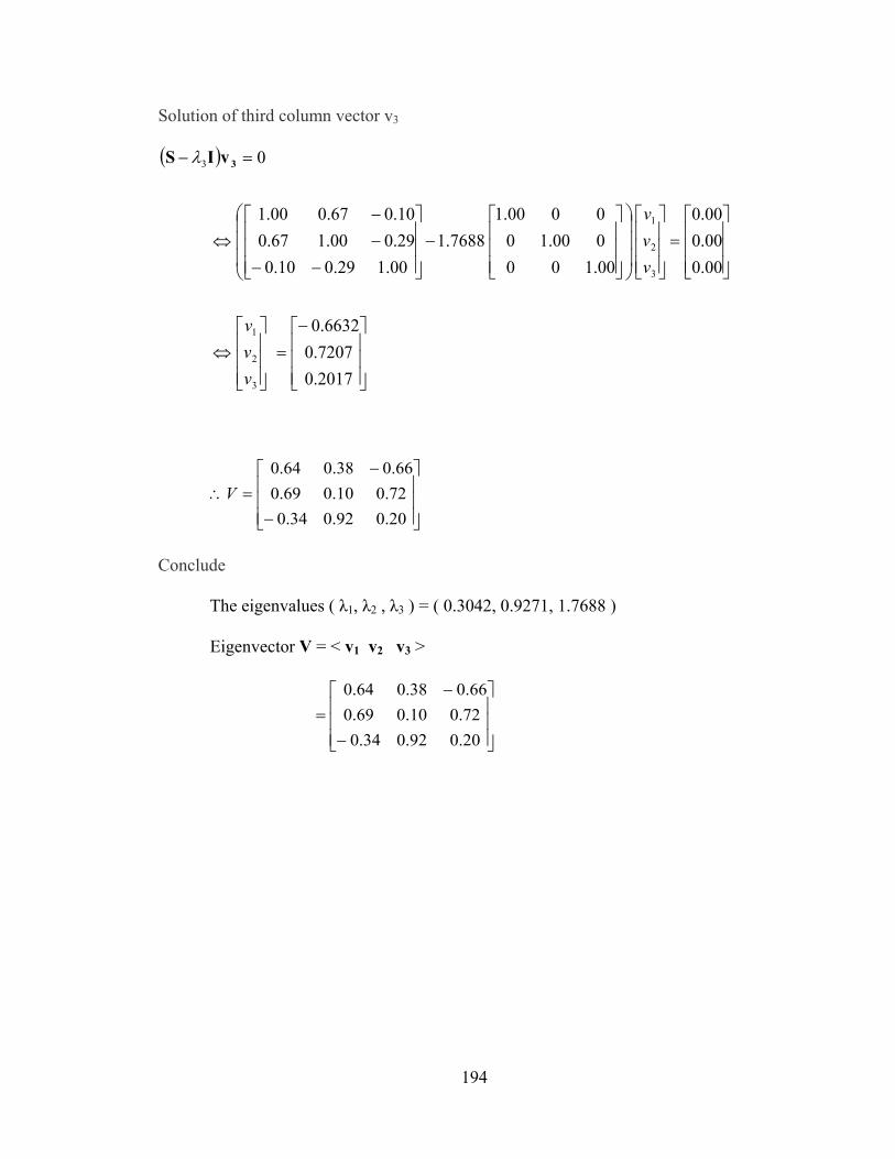
194
Solution of third column vector v3 ( )
−=
⇔
=
−
−−−−
⇔
=−
2017.07207.06632.0
00.000.000.0
00.100000.100000.1
7688.100.129.010.029.000.167.010.067.000.1
0
3
2
1
3
2
1
3
vvv
vvv
3vIS λ
−
−=∴
20.072.066.0
92.010.038.0
34.069.064.0
V
Conclude
The eigenvalues ( λ1, λ2 , λ3 ) = ( 0.3042, 0.9271, 1.7688 )
Eigenvector V = < v1 v2 v3 >
−
−=
20.072.066.0
92.010.038.0
34.069.064.0

195
Step 6 Get the factor score matrix F = Z V* , where V* = [ v1 , v2 ] as the third
principal component has been disregarded.
Pattern F1,p F2,p 1 0.51 -0.63 2 -2.66 0.06 3 -0.58 -0.29 4 2.05 -0.91 5 0.88 0.99 6 -1.08 1.21 7 -0.76 -1.20 8 1.18 1.57 9 0.27 0.02 10 0.19 -0.83
Table B.7 Data for matrix F in PCA numerical example
Recognise that in this step, we have achieved data compression by transforming matrix Z [ 10 x 3 ] into matrix F [ 10 x 2 ].

196
B.2 A Numerical Example for Artificial Neural Network using
the Gradient Descent Rule and Sigmoid Activation Function Consider
Pattern x1,p x2,p x3,p ŷp 1 0.93 0.79 0.66 0.62 2 0.83 0.80 0.63 0.54 3 0.96 0.12 0.98 1.20 4 0.71 0.84 0.03 0.03 5 0.98 0.14 0.47 0.84 6 0.59 0.98 0.72 0.37 7 0.43 0.92 0.61 0.22 8 0.03 0.90 0.48 -0.10 9 0.78 0.43 0.79 0.80 10 0.81 0.46 0.42 0.55
Table B.8 Data for matrix X in ANN numerical example
Initialisation
Set (randomly): w1 = 0.80
w2 = 0.40 w3 = 1.00
* Iteration 1 Calculate the summed weighted inputs Np for each pattern.

197
Calculate the networks output yp for each pattern
( )
( )
( )
( ) 78.01
11
1...
83.01
11
1
85.01
11
11
1
25.11510
61.122
72.111
=+
=+
==
=+
=+
==
=+
=+
==
+==
−−
−−
−−
−
eeNfy
eeNfy
eeNfy
eNfy
p
p
p
p
Nsigmoid
Nsigmoid
Nsigmoid
Npsigmoidp
Calculate the energy level E each output p
( )
( ) ( )
( ) ( )
( ) ( ) 03.078.055.021ˆ
21
...
04.083.054.021ˆ
21
03.085.062.021ˆ
21
ˆ21
22101010
22222
22111
2
=−=−=
=−=−=
=−=−=
−=
yyE
yyE
yyE
yyE ppp
( )
( )
( )
( ) 25.142.000.146.040.081.080.0
...
61.163.000.180.040.083.080.0
72.166.000.179.040.093.080.0
3
110,10
3
12,2
3
11,1
1,
=×+×+×==
=×+×+×==
=×+×+×==
=
∑
∑
∑
∑
=
=
=
=
iii
iii
iii
n
ipiip
xwN
xwN
xwN
xwN
(A.23)
(A.24)
(A.22)

198
Pattern ŷp Np Yp Ep
1 0.62 1.72 0.85 0.03 2 0.54 1.61 0.83 0.04 3 1.20 1.80 0.86 0.06 4 0.03 0.94 0.72 0.24 5 0.84 1.31 0.79 0.00 6 0.37 1.58 0.83 0.11 7 0.22 1.32 0.79 0.16 8 -0.10 0.86 0.70 0.32 9 0.80 1.58 0.83 0.00 10 0.55 1.25 0.78 0.03
Table B.9 Internal energies at first iteration in ANN numerical example
Calculate the network’s total energy ET
98.003.0...04.003.0
1
=+++=
= ∑=
P
ppT EE
Compute the weight correction coefficients δp.
( ) ( ) ( )
( ) ( ) ( ) ( ) ( ) ( )( ) ( ) ( ) ( ) ( ) ( )
( ) ( ) ( ) ( ) ( ) ( ) 04.078.055.078.0178.0ˆ1...
04.083.054.083.0183.0ˆ103.085.062.085.0185.0ˆ1
ˆ1
1010101010
22222
11111
−=−×−×=−×−×=
−=−×−×=−×−×=−=−×−×=−×−×=
−×−×=
yyyy
yyyyyyyy
yyyy ppppp
δ
δδ
δ
Compute the summed product of the weight correction coefficient δp and xi.
With respect to first variable x1,p
( )( ) ( ) ( ) 23.081.004.0...83.004.093.003.01
,1
−=×−++×−+×−=
⋅∑=
N
ppp xδ
(A.25)
(A.26)

199
With respect to second variable x2,p
( )( ) ( ) ( ) 49.046.004.0...80.004.079.003.01
,2
−=×−++×−+×−=
⋅∑=
N
ppp xδ
With respect to second variable x3,p
( )( ) ( ) ( ) 21.042.004.0...63.004.066.003.01
,3
−=×−++×−+×−=
⋅∑=
N
ppp xδ
Find the weight differential
( ) ( )
( ) ( ) ( )
( ) ( ) ( )
( ) ( ) ( ) 04.021.02.00.1
10.049.02.00.1
05.023.02.00.1
13,3
12,2
11,1
1,
−=−××=⋅=∆
−=−××=⋅=∆
−=−××=⋅=∆
⋅=∆
∑
∑
∑
∑
=
=
=
=
P
ppp
P
ppp
P
ppp
P
pippi
xtw
xtw
xtw
xtw
δηα
δηα
δηα
δηα
Correct the weights ( ) ( ) ( )
( ) ( ) ( )( ) ( ) ( )( ) ( ) ( ) 96.004.000.11
30.010.040.0175.005.080.01
1
333
222
111
=−=∆+=+=−=∆+=+=−=∆+=+
∆+=+
twtwtwtwtwtw
twtwtw
twtwtw iii
(A.27)
(A.28)

200
Reset : w1 = 0.75
w2 = 0.30 w3 = 0.96
Summary
Iteration w1 w2 w3 ET 0 0.80 0.40 1.00 0.98 1 0.75 0.30 0.96 0.91 2 0.71 0.20 0.92 0.85 3 0.67 0.10 0.88 0.78 4 0.63 0.01 0.84 0.72 5 0.59 -0.09 0.80 0.66 6 0.56 -0.18 0.77 0.61 7 0.53 -0.27 0.75 0.56 8 0.51 -0.36 0.72 0.53 9 0.49 -0.43 0.70 0.50 10 0.48 -0.51 0.69 0.47
Table B.10 Weight correction up to 10 iterations in ANN numerical example

201
Appendix C Completeness of the Data
Table C.1 Completeness of the data for air pollution readings at Airport station
Month O3 (Airport) PM2.5 (Airport) NO (Airport) NO2 (Airport) CO (Airport)Jan-04 0% 100% 100% 100% 100%Feb-04 0% 99% 100% 100% 100%Mar-04 0% 99% 36% 100% 97%Apr-04 0% 99% 100% 100% 100%May-04 0% 85% 85% 85% 85%Jun-04 46% 0% 48% 46% 48%Jul-04 99% 36% 99% 99% 99%Aug-04 94% 95% 99% 99% 99%Sep-04 99% 95% 99% 99% 99%Oct-04 100% 100% 100% 100% 96%Nov-04 98% 100% 98% 98% 98%Dec-04 100% 95% 100% 100% 100%Jan-05 100% 100% 100% 100% 100%Feb-05 100% 94% 100% 100% 100%Mar-05 100% 95% 100% 100% 100%Apr-05 100% 98% 99% 96% 100%May-05 99% 99% 99% 99% 96%Jun-05 100% 85% 100% 100% 100%Jul-05 100% 89% 100% 100% 100%Aug-05 100% 97% 100% 100% 100%Sep-05 100% 100% 100% 100% 100%Oct-05 100% 98% 100% 100% 100%Nov-05 99% 95% 99% 99% 99%Dec-05 100% 100% 100% 100% 100%Jan-06 100% 98% 100% 100% 100%Feb-06 100% 99% 100% 100% 98%Mar-06 100% 98% 100% 100% 95%Apr-06 100% 100% 100% 100% 100%May-06 100% 98% 100% 100% 100%Jun-06 100% 97% 100% 100% 100%Jul-06 99% 99% 99% 99% 99%Aug-06 100% 99% 100% 100% 99%Sep-06 99% 98% 99% 99% 99%Oct-06 100% 100% 100% 100% 100%Nov-06 99% 96% 98% 98% 98%Dec-06 99% 99% 99% 99% 97%Jan-07 100% 99% 100% 100% 100%Feb-07 100% 99% 94% 94% 100%Mar-07 100% 100% 100% 100% 100%Apr-07 100% 100% 100% 100% 100%May-07 99% 99% 99% 99% 98%Jun-07 99% 97% 99% 99% 100%Jul-07 99% 96% 99% 99% 99%Aug-07 100% 96% 100% 100% 100%Sep-07 100% 98% 100% 100% 100%Oct-07 99% 95% 100% 100% 100%Nov-07 100% 92% 100% 100% 100%Dec-07 99% 99% 99% 99% 94%

202
Table C.2 Completeness of the data for air pollution readings at Maisonneuve station
Month SR Temp DP Press Precip WS WDJan-04 100% 100% 100% 100% 100% 100% 100%Feb-04 100% 100% 100% 100% 100% 100% 100%Mar-04 100% 100% 100% 100% 99% 100% 100%Apr-04 100% 99% 99% 100% 99% 99% 99%May-04 100% 100% 99% 99% 99% 100% 100%Jun-04 100% 100% 99% 100% 100% 100% 100%Jul-04 100% 100% 91% 91% 91% 100% 100%Aug-04 76% 99% 99% 100% 99% 99% 99%Sep-04 100% 100% 99% 98% 98% 100% 100%Oct-04 99% 100% 95% 100% 100% 100% 100%Nov-04 98% 93% 93% 93% 93% 93% 93%Dec-04 100% 100% 100% 100% 100% 100% 100%Jan-05 100% 100% 100% 99% 99% 100% 100%Feb-05 100% 99% 99% 100% 100% 99% 99%Mar-05 100% 94% 94% 93% 93% 94% 94%Apr-05 100% 92% 92% 68% 68% 92% 92%May-05 100% 100% 100% 100% 100% 100% 100%Jun-05 100% 100% 99% 99% 99% 100% 100%Jul-05 100% 100% 100% 100% 99% 100% 100%Aug-05 100% 100% 97% 100% 100% 100% 100%Sep-05 99% 100% 100% 99% 99% 100% 100%Oct-05 100% 100% 97% 100% 99% 100% 100%Nov-05 100% 73% 70% 73% 73% 73% 73%Dec-05 100% 100% 100% 100% 100% 100% 100%Jan-06 100% 100% 100% 96% 95% 100% 100%Feb-06 100% 100% 96% 96% 96% 100% 100%Mar-06 100% 100% 100% 100% 100% 100% 100%Apr-06 100% 100% 100% 100% 100% 100% 100%May-06 100% 100% 100% 99% 100% 100% 100%Jun-06 100% 100% 100% 100% 100% 100% 100%Jul-06 100% 100% 100% 100% 100% 100% 100%Aug-06 97% 100% 100% 100% 100% 100% 100%Sep-06 67% 100% 100% 100% 100% 100% 100%Oct-06 0% 100% 100% 97% 97% 100% 100%Nov-06 48% 100% 100% 100% 100% 100% 0%Dec-06 100% 100% 100% 100% 100% 100% 100%Jan-07 99% 100% 100% 100% 100% 100% 100%Feb-07 55% 100% 100% 100% 100% 100% 100%Mar-07 0% 100% 100% 100% 100% 100% 100%Apr-07 0% 100% 100% 97% 97% 100% 100%May-07 0% 100% 100% 97% 97% 100% 100%Jun-07 100% 100% 100% 100% 100% 100% 100%Jul-07 99% 100% 97% 83% 83% 100% 100%Aug-07 100% 100% 78% 100% 100% 100% 100%Sep-07 100% 100% 100% 100% 100% 100% 100%Oct-07 30% 100% 99% 99% 98% 100% 100%Nov-07 0% 100% 99% 100% 100% 100% 100%Dec-07 0% 100% 98% 100% 92% 100% 100%

203
Table C.3 Completeness of the data for meteorological readings at Airport station
Month SR Temp DP Press Precip WS WDJan-04 100% 100% 100% 100% 100% 100% 100%Feb-04 100% 100% 100% 100% 100% 100% 100%Mar-04 100% 100% 100% 100% 99% 100% 100%Apr-04 100% 99% 99% 100% 99% 99% 99%May-04 100% 100% 99% 99% 99% 100% 100%Jun-04 100% 100% 99% 100% 100% 100% 100%Jul-04 100% 100% 91% 91% 91% 100% 100%Aug-04 76% 99% 99% 100% 99% 99% 99%Sep-04 100% 100% 99% 98% 98% 100% 100%Oct-04 99% 100% 95% 100% 100% 100% 100%Nov-04 98% 93% 93% 93% 93% 93% 93%Dec-04 100% 100% 100% 100% 100% 100% 100%Jan-05 100% 100% 100% 99% 99% 100% 100%Feb-05 100% 99% 99% 100% 100% 99% 99%Mar-05 100% 94% 94% 93% 93% 94% 94%Apr-05 100% 92% 92% 68% 68% 92% 92%May-05 100% 100% 100% 100% 100% 100% 100%Jun-05 100% 100% 99% 99% 99% 100% 100%Jul-05 100% 100% 100% 100% 99% 100% 100%Aug-05 100% 100% 97% 100% 100% 100% 100%Sep-05 99% 100% 100% 99% 99% 100% 100%Oct-05 100% 100% 97% 100% 99% 100% 100%Nov-05 100% 73% 70% 73% 73% 73% 73%Dec-05 100% 100% 100% 100% 100% 100% 100%Jan-06 100% 100% 100% 96% 95% 100% 100%Feb-06 100% 100% 96% 96% 96% 100% 100%Mar-06 100% 100% 100% 100% 100% 100% 100%Apr-06 100% 100% 100% 100% 100% 100% 100%May-06 100% 100% 100% 99% 100% 100% 100%Jun-06 100% 100% 100% 100% 100% 100% 100%Jul-06 100% 100% 100% 100% 100% 100% 100%Aug-06 97% 100% 100% 100% 100% 100% 100%Sep-06 67% 100% 100% 100% 100% 100% 100%Oct-06 0% 100% 100% 97% 97% 100% 100%Nov-06 48% 100% 100% 100% 100% 100% 0%Dec-06 100% 100% 100% 100% 100% 100% 100%Jan-07 99% 100% 100% 100% 100% 100% 100%Feb-07 55% 100% 100% 100% 100% 100% 100%Mar-07 0% 100% 100% 100% 100% 100% 100%Apr-07 0% 100% 100% 97% 97% 100% 100%May-07 0% 100% 100% 97% 97% 100% 100%Jun-07 100% 100% 100% 100% 100% 100% 100%Jul-07 99% 100% 97% 83% 83% 100% 100%Aug-07 100% 100% 78% 100% 100% 100% 100%Sep-07 100% 100% 100% 100% 100% 100% 100%Oct-07 30% 100% 99% 99% 98% 100% 100%Nov-07 0% 100% 99% 100% 100% 100% 100%Dec-07 0% 100% 98% 100% 92% 100% 100%

204
APPENDIX D: Monthly Averages (2004 – 2007 Time Series) D.1 Air Quality Data at Airport
Table D.1 Monthly averages (2004 – 2007) of air quality data at Airport
Month O3 (Airport) PM2.5 (Airport) NO (Airport) NO2 (Airport) CO (Airport)Jan-04 5.8 7.3 28.2 335.2Feb-04 11.0 22.5 50.0 424.5Mar-04 9.0 28.2 41.3 421.5Apr-04 5.6 2.9 27.5 297.3May-04 7.6 5.1 24.9 254.9Jun-04 45.4 2.1 19.1 173.2Jul-04 41.7 10.5 3.6 21.1 282.3Aug-04 36.3 10.1 4.5 18.8 308.0Sep-04 30.8 7.6 9.6 21.8 220.5Oct-04 28.5 7.2 18.3 28.7 227.0Nov-04 23.4 7.0 21.9 32.9 238.5Dec-04 32.5 8.3 17.7 35.1 260.5Jan-05 33.2 8.4 13.1 38.5 284.7Feb-05 31.2 18.9 30.7 54.9 466.7Mar-05 57.9 6.7 6.6 30.9 210.3Apr-05 58.6 5.5 5.0 26.5 212.9May-05 54.7 5.1 4.8 21.0 200.2Jun-05 61.3 17.1 4.7 22.0 377.8Jul-05 52.1 9.4 3.1 17.5 320.7Aug-05 51.6 10.3 3.7 17.4 378.7Sep-05 45.0 9.4 3.4 16.9 334.8Oct-05 29.1 7.8 6.8 22.0 325.6Nov-05 29.4 6.9 11.8 25.7 350.8Dec-05 30.4 7.1 13.4 32.3 378.7Jan-06 27.2 9.8 19.0 39.2 473.4Feb-06 44.9 6.6 8.3 28.2 385.5Mar-06 55.7 5.9 5.0 24.0 357.7Apr-06 57.6 4.2 3.2 21.0 366.4May-06 52.7 6.8 3.8 20.7 334.0Jun-06 51.4 7.9 2.7 17.9 305.4Jul-06 60.6 10.5 1.4 14.2 382.4Aug-06 43.2 6.8 3.6 15.8 346.7Sep-06 32.4 6.1 5.0 16.2 339.0Oct-06 29.4 4.3 8.6 19.9 296.2Nov-06 21.0 8.0 16.9 25.0 404.3Dec-06 31.1 5.4 7.1 24.5 326.0Jan-07 37.9 6.1 9.2 26.0 350.4Feb-07 46.6 6.2 7.8 26.4 326.7Mar-07 49.3 5.9 9.0 27.9 335.4Apr-07 53.4 4.7 3.6 23.0 273.7May-07 64.9 7.5 2.6 18.9 324.9Jun-07 60.4 9.0 2.2 15.5 349.0Jul-07 52.6 9.4 2.5 15.2 354.0Aug-07 47.8 7.6 5.5 17.3 346.5Sep-07 46.3 7.2 4.5 16.5 322.3Oct-07 33.9 6.2 12.6 23.3 360.8Nov-07 36.0 5.3 10.2 24.1 315.3Dec-07 35.2 6.0 11.5 32.7 326.4

205
D.2 Air Quality Data at Maisonneuve
Table D.2 Monthly averages (2004 – 2007) of air quality data at Maisonneuve
Month O3 (Maison) PM2.5 (Maison) NO (Maison) NO2 (Maison) CO (Maison)Jan-04 26.1 5.9 41.5 40.8 467.3Feb-04 21.3 10.3 51.5 50.8 560.7Mar-04 26.7 8.7 42.3 62.9 503.7Apr-04 32.5 6.5 33.7 55.9 441.5May-04 29.2 8.1 30.8 52.3 413.7Jun-04 36.4 8.9 23.2 41.8 402.4Jul-04 31.7 11.2 19.2 39.7 350.5Aug-04 25.1 11.3 25.0 40.0 394.8Sep-04 19.1 10.0 34.1 41.4 445.1Oct-04 13.9 7.9 42.3 44.3 456.5Nov-04 11.9 7.5 49.9 45.0 495.1Dec-04 18.6 9.2 41.9 47.4 502.4Jan-05 20.3 8.7 41.7 53.1 511.4Feb-05 19.2 18.2 60.2 67.4 649.1Mar-05 37.3 7.9 29.8 55.4 418.7Apr-05 39.3 6.9 24.3 49.1 426.6May-05 35.5 6.7 22.9 41.1 389.9Jun-05 40.7 15.7 19.3 39.6 531.8Jul-05 36.1 12.2 15.2 34.0 530.0Aug-05 34.4 12.0 19.5 41.9 558.6Sep-05 28.1 11.4 21.9 38.9 525.0Oct-05 17.9 11.3 29.9 38.6 518.3Nov-05 15.9 7.9 35.6 44.0 613.9Dec-05 16.2 7.5 36.5 46.9 572.8Jan-06 17.3 9.9 40.7 51.5 623.5Feb-06 25.8 7.5 30.5 48.6 569.6Mar-06 31.8 8.1 28.4 52.1 532.7Apr-06 38.0 5.5 18.7 41.8 450.2May-06 36.3 8.0 19.4 37.0 480.8Jun-06 33.5 7.0 19.9 36.7 561.0Jul-06 42.3 14.4 34.5 559.2Aug-06 27.5 21.4 33.8 583.2Sep-06 18.9 9.7 24.1 33.5 532.3Oct-06 18.4 7.4 31.5 36.6 515.0Nov-06 12.2 9.0 40.1 41.0 602.6Dec-06 18.2 6.2 30.5 41.4 517.6Jan-07 22.6 6.0 29.6 41.9 509.1Feb-07 30.7 6.9 29.4 48.6 380.3Mar-07 32.7 6.4 27.8 45.6 355.7Apr-07 39.3 5.6 18.1 26.5 277.5May-07 47.1 8.3 17.4 40.1 273.1Jun-07 39.4 10.2 19.4 37.6 404.8Jul-07 36.3 10.8 14.7 34.6 392.8Aug-07 31.1 7.3 18.5 35.9 400.5Sep-07 30.6 8.8 16.8 34.2 384.4Oct-07 19.9 6.4 29.8 42.1 454.2Nov-07 20.4 5.1 26.1 42.2 338.1Dec-07 21.4 5.7 27.6 45.1 140.3

206
D.3 Meteorological Data at Airport
Table D.3 Monthly averages (2004 – 2007) of meteorological data at Airport
Month SR Temp DP Press PrecipJan-04 553.3 -14.8 -20.0 101.0 0.0Feb-04 460.6 -7.1 -12.7 101.6 0.0Mar-04 252.6 0.1 -6.8 101.5 0.1Apr-04 164.7 6.2 -3.2 101.0 0.1May-04 214.7 14.0 6.9 101.1 0.1Jun-04 357.1 17.9 10.6 101.0 0.1Jul-04 631.4 21.6 16.0 100.9 0.2Aug-04 695.2 19.6 14.5 101.1 0.1Sep-04 767.0 16.5 11.5 101.6 0.1Oct-04 883.6 9.3 4.5 101.2 0.0Nov-04 1201.0 2.2 -2.0 101.5 0.1Dec-04 808.0 -7.1 -10.1 101.2 0.2Jan-05 626.8 -10.8 -15.6 102.0 0.1Feb-05 328.6 -6.2 -10.9 101.6 0.1Mar-05 193.0 -2.9 -9.8 100.6 0.1Apr-05 166.7 7.8 -1.1 100.9 0.3May-05 149.2 11.9 4.4 101.2 0.1Jun-05 269.7 21.7 14.7 100.9 0.2Jul-05 435.6 22.7 15.7 101.1 0.2Aug-05 615.6 22.0 15.6 101.1 0.2Sep-05 643.6 17.8 12.6 101.3 0.1Oct-05 759.1 10.2 6.3 101.2 0.2Nov-05 838.1 4.4 0.1 101.0 0.1Dec-05 741.8 -5.2 -8.4 101.0 0.1Jan-06 515.7 -4.5 -7.6 100.9 0.2Feb-06 308.7 -6.9 -12.3 100.8 0.1Mar-06 168.1 -0.6 -7.5 101.0 0.0Apr-06 138.1 8.0 -0.7 101.0 0.1May-06 165.3 14.6 8.2 100.7 0.2Jun-06 319.3 19.5 12.9 100.9 0.1Jul-06 446.7 22.9 16.1 100.9 0.1Aug-06 468.4 19.7 12.9 101.1 0.2Sep-06 596.1 15.4 10.9 101.1 0.1Oct-06 8.1 4.2 100.8 0.2Nov-06 590.3 4.6 1.4 101.5 0.1Dec-06 600.9 -0.8 -4.2 101.4 0.1Jan-07 502.8 -6.9 -11.5 101.1 0.1Feb-07 396.9 -10.6 -16.4 100.8 0.0Mar-07 -2.4 -9.1 101.5 0.1Apr-07 5.9 -0.6 100.7 0.2May-07 14.1 4.4 101.5 0.1Jun-07 115.3 20.1 12.8 100.9 0.1Jul-07 125.8 20.6 15.2 100.9 0.2Aug-07 145.3 20.5 14.3 101.0 0.1Sep-07 501.1 17.2 11.3 101.4 0.1Oct-07 411.6 11.6 7.5 101.2 0.1Nov-07 1.4 -2.7 101.2 0.2Dec-07 -6.0 -9.0 101.4
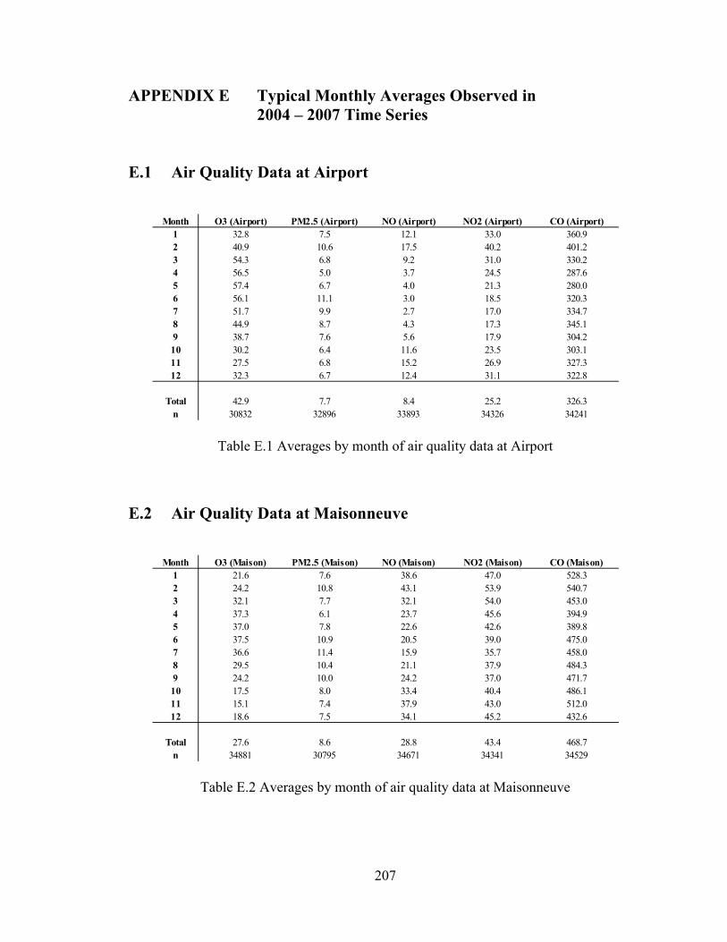
207
APPENDIX E Typical Monthly Averages Observed in 2004 – 2007 Time Series
E.1 Air Quality Data at Airport
Table E.1 Averages by month of air quality data at Airport
E.2 Air Quality Data at Maisonneuve
Table E.2 Averages by month of air quality data at Maisonneuve
Month O3 (Airport) PM2.5 (Airport) NO (Airport) NO2 (Airport) CO (Airport)1 32.8 7.5 12.1 33.0 360.92 40.9 10.6 17.5 40.2 401.23 54.3 6.8 9.2 31.0 330.24 56.5 5.0 3.7 24.5 287.65 57.4 6.7 4.0 21.3 280.06 56.1 11.1 3.0 18.5 320.37 51.7 9.9 2.7 17.0 334.78 44.9 8.7 4.3 17.3 345.19 38.7 7.6 5.6 17.9 304.210 30.2 6.4 11.6 23.5 303.111 27.5 6.8 15.2 26.9 327.312 32.3 6.7 12.4 31.1 322.8
Total 42.9 7.7 8.4 25.2 326.3n 30832 32896 33893 34326 34241
Month O3 (Maison) PM2.5 (Maison) NO (Maison) NO2 (Maison) CO (Maison)1 21.6 7.6 38.6 47.0 528.32 24.2 10.8 43.1 53.9 540.73 32.1 7.7 32.1 54.0 453.04 37.3 6.1 23.7 45.6 394.95 37.0 7.8 22.6 42.6 389.86 37.5 10.9 20.5 39.0 475.07 36.6 11.4 15.9 35.7 458.08 29.5 10.4 21.1 37.9 484.39 24.2 10.0 24.2 37.0 471.710 17.5 8.0 33.4 40.4 486.111 15.1 7.4 37.9 43.0 512.012 18.6 7.5 34.1 45.2 432.6
Total 27.6 8.6 28.8 43.4 468.7n 34881 30795 34671 34341 34529

208
E.3 Meteorological Data at Airport
Table E.3 Averages by month of meteorological data at Airport
Month SR Temp DP Press Precip1 549.7 -9.2 -13.7 101.3 0.12 371.7 -7.7 -13.1 101.2 0.13 204.6 -1.4 -8.3 101.2 0.14 156.5 7.0 -1.4 100.9 0.25 176.4 13.7 5.9 101.1 0.16 265.3 19.8 12.7 100.9 0.17 410.2 21.9 15.8 100.9 0.28 467.8 20.4 14.3 101.1 0.29 629.7 16.7 11.6 101.3 0.110 767.0 9.8 5.6 101.1 0.211 934.7 3.1 -0.9 101.3 0.112 717.0 -4.8 -7.9 101.3 0.7
Total 456.2 7.6 1.7 101.1 0.2n 28963 34692 34239 34145 34042

209
APPENDIX F Hourly Averages (2004 – 2007 Time Series) by Season
Table F.1 Hourly averages of air quality data at Airport (summer)
Table F.2 Hourly averages of air quality data at Airport (winter)
Hour O3 (Airport) PM2.5 (Airport) NO (Airport) NO2 (Airport) CO (Airport)0 41.4 8.8 2.5 21.8 329.91 40.6 8.9 3.0 20.5 316.12 38.7 9.0 2.2 19.8 308.03 36.1 9.2 2.3 20.7 306.04 33.4 9.6 3.9 22.5 310.05 32.5 10.2 7.3 24.2 338.36 36.1 10.1 9.7 23.9 351.27 41.9 9.8 8.9 21.7 346.98 49.3 9.3 6.7 18.9 331.69 57.3 9.1 4.8 15.6 312.910 66.9 9.0 2.9 12.3 296.711 73.1 8.6 2.2 10.9 279.312 77.3 8.3 2.1 10.5 275.513 78.5 8.3 2.0 10.8 275.014 79.4 8.3 2.0 11.0 276.015 79.0 8.1 1.7 11.2 268.216 76.7 8.0 1.7 13.2 277.117 73.9 8.4 1.5 15.2 285.818 68.2 8.7 1.1 17.8 299.119 57.1 9.1 1.4 25.3 321.320 50.0 9.7 1.2 26.9 340.921 45.1 9.4 2.1 28.0 344.622 42.4 9.0 2.4 26.4 347.323 41.3 8.8 2.5 24.2 341.7
Total 54.8 9.0 3.3 18.9 311.7n 7652 7228 8297 8278 8279
Hour O3 (Airport) PM2.5 (Airport) NO (Airport) NO2 (Airport) CO (Airport)0 28.4 7.6 11.1 30.7 345.71 29.2 7.4 10.8 29.2 323.82 29.5 6.9 10.1 28.0 314.53 29.4 6.3 9.3 27.4 295.64 29.1 6.0 9.2 27.3 281.65 26.9 6.0 10.4 29.3 283.86 24.1 6.5 14.8 33.7 325.77 22.8 7.1 20.1 36.5 370.98 26.8 7.4 22.6 33.3 384.09 31.9 6.9 20.9 28.9 367.810 36.5 6.1 17.7 24.0 310.811 39.4 5.7 16.2 22.6 297.712 41.5 5.9 13.8 21.3 292.413 41.5 6.2 12.6 22.6 287.714 40.5 6.7 11.6 24.3 311.915 37.1 6.6 11.1 27.7 326.516 31.3 6.7 11.2 33.4 347.717 28.0 7.3 11.9 36.8 388.418 27.3 7.8 12.1 37.2 384.919 27.3 8.0 12.5 36.4 380.220 27.3 8.2 12.6 36.1 369.321 27.3 8.5 11.7 34.7 371.222 27.3 8.3 11.6 33.8 365.423 27.5 8.0 12.0 32.8 363.5
Total 30.7 7.0 13.2 30.4 337.2n 8030 8627 8770 8770 8720

210
Table F.3 Hourly averages of air quality data at Maisonneuve (Summer)
Table F.4 Hourly averages of air quality data at Maisonneuve (Winter)
Hour O3 (Maison) PM2.5 (Maison) NO (Maison) NO2 (Maison) CO (Maison)0 33.9 7.6 11.2 34.1 364.11 35.3 7.6 8.9 30.4 327.42 33.8 7.6 9.2 30.1 316.33 34.4 7.8 6.7 27.3 227.74 30.8 8.0 8.8 29.1 228.05 25.0 8.4 19.6 35.9 289.16 21.2 9.2 31.6 42.0 382.37 23.3 9.4 35.4 43.1 440.38 27.7 9.2 33.9 42.8 431.89 32.9 8.8 29.8 41.8 473.610 40.7 9.5 27.2 40.5 463.011 47.2 10.5 23.0 38.0 487.112 51.1 9.6 21.4 37.9 465.513 51.5 8.9 21.5 39.2 465.414 50.1 8.9 21.1 40.7 482.215 48.4 9.5 21.5 42.7 542.816 45.2 10.3 22.1 45.3 598.517 47.1 12.0 17.8 41.5 535.218 46.0 13.9 14.2 39.6 508.119 39.6 15.0 15.4 42.7 525.520 32.1 15.0 20.5 47.0 561.821 30.5 12.0 19.1 45.5 511.622 29.7 9.4 17.2 42.8 499.623 31.1 8.0 15.1 38.9 455.1
Total 37.0 9.8 19.6 39.1 440.7n 8777 7222 8676 8676 8772
Hour O3 (Maison) PM2.5 (Maison) NO (Maison) NO2 (Maison) CO (Maison)0 19.8 5.9 22.6 40.6 425.31 21.1 5.9 20.6 39.0 336.22 22.1 5.3 20.2 37.6 298.63 22.5 4.9 17.5 36.3 287.64 23.3 4.5 15.8 35.2 222.25 21.8 4.6 17.8 36.6 226.36 18.4 5.1 26.0 41.6 280.57 15.0 5.9 41.1 47.2 378.08 15.1 6.6 53.3 49.1 452.49 16.7 6.7 54.0 48.5 471.610 18.6 6.6 55.5 47.2 524.811 19.6 7.2 54.5 47.0 541.412 21.4 8.3 47.5 45.2 574.113 21.3 8.4 47.1 46.1 582.814 20.5 7.3 47.6 47.1 588.215 17.8 7.4 47.8 49.7 636.116 15.1 8.1 48.9 52.0 737.917 13.6 9.7 49.2 53.2 784.418 14.5 11.3 42.4 51.4 678.419 15.9 11.7 35.0 48.7 615.020 16.9 11.9 32.9 47.4 566.321 16.5 10.6 33.8 47.3 577.022 17.4 8.7 29.9 45.3 513.423 18.4 6.9 25.4 43.0 483.1
Total 18.5 7.5 36.8 45.1 490.4n 8761 8252 8678 8678 8660

211
Table F.5 Hourly averages of meteorological data at Airport (Summer)
Table F.6 Hourly averages of meteorological data at Airport (Winter)
Hour SR Temp DP Press Precip0 1.0 16.4 11.1 101.0 0.11 1.0 15.9 11.1 101.0 0.12 1.0 15.4 11.0 101.0 0.13 0.9 15.0 10.9 101.0 0.14 0.9 14.6 10.8 101.0 0.15 0.9 14.5 10.8 101.0 0.16 1.2 15.4 11.1 101.0 0.17 20.6 16.3 11.2 101.1 0.18 143.7 17.3 11.5 101.1 0.19 427.2 18.3 11.7 101.1 0.110 734.8 19.3 11.9 101.1 0.111 985.2 20.2 12.0 101.1 0.112 1122.7 21.0 12.0 101.0 0.213 1138.8 21.5 11.9 101.0 0.114 1011.3 21.9 11.9 101.0 0.115 776.9 22.1 11.7 100.9 0.216 475.0 22.0 11.6 100.9 0.217 179.7 21.7 11.6 100.9 0.218 30.8 21.2 11.5 100.9 0.219 1.7 20.3 11.4 100.9 0.120 1.3 19.3 11.4 100.9 0.121 1.2 18.5 11.5 101.0 0.122 1.1 17.7 11.4 101.0 0.123 1.1 17.1 11.3 101.0 0.1
Total 294.0 18.5 11.4 101.0 0.1n 8080 8832 8722 8596 8589
Hour SR Temp DP Press Precip0 0.4 -4.2 -7.8 101.3 1.11 0.4 -4.4 -7.8 101.3 0.72 0.4 -4.6 -7.9 101.3 0.13 0.4 -4.7 -7.9 101.3 0.14 0.4 -4.8 -8.0 101.3 0.15 10.6 -5.0 -8.1 101.3 0.16 134.8 -5.1 -8.2 101.3 0.17 449.4 -5.2 -8.2 101.3 0.18 855.3 -5.1 -8.1 101.3 0.19 1301.1 -4.5 -7.9 101.3 0.210 1680.1 -4.0 -7.8 101.3 0.111 1949.1 -3.4 -7.6 101.3 0.112 2076.4 -2.9 -7.5 101.2 0.113 2063.1 -2.6 -7.5 101.2 0.114 1883.8 -2.4 -7.3 101.2 0.115 1657.3 -2.4 -7.3 101.2 0.216 1279.2 -2.6 -7.4 101.2 0.717 857.7 -3.0 -7.5 101.3 0.518 449.6 -3.2 -7.5 101.3 0.619 142.2 -3.5 -7.7 101.3 0.720 15.8 -3.7 -7.7 101.3 0.421 0.5 -3.9 -7.8 101.3 0.522 0.4 -4.1 -7.9 101.3 0.723 0.4 -4.3 -7.9 101.3 0.3
Total 700.8 -3.9 -7.8 101.3 0.3n 6964 8584 8538 8541 8470

212
APPENDIX G O3 and PM2.5 Averages at Airport and Maisonneuve by Wind Direction (2004 – 2007 Time Series)
Table G.1 O3 and PM2.5 Averages by Wind Direction
Season Period WD O3 (Airport) O3 (Maison) PM2.5 (Airport) PM2.5 (Maison)0 61.4 34.3 6.0 8.31 62.2 40.0 6.5 7.62 74.2 52.7 7.5 8.43 79.6 53.3 9.7 11.84 85.9 54.2 9.5 11.65 93.3 62.1 11.5 12.66 68.9 40.8 5.8 6.87 60.8 31.4 4.5 6.28 86.6 49.5 10.2 11.30 28.2 24.7 6.7 5.31 31.3 26.9 7.6 6.22 34.7 35.8 8.3 6.73 36.5 30.5 10.1 9.24 49.5 37.0 13.3 12.15 52.9 42.7 11.0 10.66 44.5 36.5 7.8 7.47 28.1 22.5 4.9 4.18 16.4 22.3 12.0 9.30 28.5 14.2 13.0 14.71 26.4 19.0 9.4 9.72 29.8 23.0 5.1 5.23 41.1 19.8 4.9 8.04 39.0 13.4 5.4 8.65 40.5 17.7 6.6 7.46 50.8 24.7 3.2 4.87 45.9 17.7 3.4 5.28 31.4 13.8 12.6 15.20 21.0 16.2 11.9 9.41 22.3 21.4 7.8 6.12 20.6 22.6 7.0 6.33 32.4 18.7 5.5 6.04 28.4 11.3 7.3 8.05 30.7 19.3 7.4 6.26 38.0 27.0 4.7 3.67 39.0 25.5 6.3 4.98 9.8 12.4 14.2 9.6
Day
Night
Summer
Day
Night
Winter

213
APPENDIX H Hourly Averages by Season by Period (2004 – 2007 Time Series)
H.1 Summer
Table H.1 Hourly averages of air quality data at Airport (summer/day)
Summer/Day O3 (Airport) PM2.5 (Airport) NO (Airport) NO2 (Airport) CO (Airport)Moments
Mean 77.3 8.3 1.9 11.3 275.2Std Dev 28.8 8.5 3.0 8.1 117.1
Std Err Mean 0.7 0.2 0.1 0.2 2.6upper 95% Mean 78.6 8.7 2.1 11.6 280.2lower 95% Mean 76.1 7.9 1.8 10.9 270.1
Variance 827.4 72.2 8.7 65.7 13712.6Skewness 0.2 1.9 6.4 1.6 0.2
Kurtosis 0.1 4.4 65.1 4.0 0.3n 1903.0 1789.0 2062.0 2058.0 2058.0
Percentiles100.0% 170.0 55.0 46.0 77.0 799.999.5% 162.5 44.0 21.7 41.7 599.997.5% 137.4 33.0 8.0 33.0 499.990.0% 115.0 19.0 4.0 22.0 399.975.0% 96.0 11.0 2.0 15.0 399.950.0% 76.0 5.0 1.0 9.0 300.025.0% 58.0 3.0 1.0 6.0 200.010.0% 43.0 1.0 0.0 3.0 100.02.5% 21.0 0.0 0.0 2.0 100.00.5% 9.5 0.0 0.0 1.0 0.00.0% 5.0 0.0 0.0 0.0 0.0

214
Table H.2 Hourly averages of air quality data at Maisonneuve (summer/day)
Summer/Day O3 (Maison) PM2.5 (Maison) NO (Maison) NO2 (Maison) CO (Maison)Moments
Mean 48.9 9.6 21.8 40.6 507.2Std Dev 23.7 8.7 14.5 15.1 230.1
Std Err Mean 0.5 0.2 0.3 0.3 4.9upper 95% Mean 49.9 10.0 22.4 41.3 516.8lower 95% Mean 47.9 9.2 21.2 40.0 497.5
Variance 560.6 76.2 209.0 229.3 52944.7Skewness 0.4 1.7 1.6 0.7 0.6
Kurtosis 0.4 3.5 4.1 1.0 0.8n 2192.0 1793.0 2168.0 2168.0 2190.0
Percentiles100.0% 145.0 54.0 122.0 119.0 1799.799.5% 127.1 46.0 84.0 94.2 1204.397.5% 98.0 33.0 61.0 73.8 999.890.0% 78.0 22.0 40.0 60.0 799.975.0% 65.0 13.0 29.0 50.0 699.950.0% 48.0 7.0 18.0 40.0 499.925.0% 32.0 3.0 11.0 29.0 299.910.0% 19.0 2.0 7.0 22.0 200.02.5% 6.0 0.0 4.0 15.0 100.00.5% 1.0 0.0 2.0 12.9 100.00.0% 0.0 0.0 1.0 10.0 0.0

215
Table H.3 Hourly averages of meteorological data at Airport (summer/day)
Table H.4 Hourly averages of air quality data at Airport (summer/night)
Summer/Day SR Temp DP Press Precip WS WDIMoments
Mean 918.7 21.5 11.9 101.0 0.1 17.8 1.3Std Dev 667.1 5.8 6.3 0.6 0.9 8.3 0.7
Std Err Mean 14.9 0.1 0.1 0.0 0.0 0.2 0.0upper 95% Mean 947.9 21.7 12.1 101.0 0.2 18.2 1.3lower 95% Mean 889.6 21.2 11.6 101.0 0.1 17.5 1.3
Variance 445034.6 33.1 39.2 0.4 0.8 68.9 0.5Skewness 0.6 -0.5 -0.8 -0.2 11.4 0.5 -0.8
Kurtosis -0.5 -0.4 0.3 0.6 171.9 0.0 -1.0n 2017.0 2208.0 2177.0 2144.0 2143.0 2208.0 2208.0
Percentiles100.0% 2804.0 32.7 23.2 103.1 19.3 52.0 2.099.5% 2739.6 32.0 22.5 102.7 6.0 42.9 2.097.5% 2389.2 30.6 21.1 102.3 1.8 37.0 2.090.0% 1888.2 28.4 19.0 101.7 0.0 30.0 2.075.0% 1382.5 25.8 16.8 101.4 0.0 24.0 2.050.0% 818.0 22.4 12.7 101.0 0.0 17.0 1.725.0% 328.0 17.6 8.2 100.6 0.0 11.0 1.010.0% 138.0 12.7 3.4 100.2 0.0 7.0 0.02.5% 61.4 9.2 -3.2 99.6 0.0 4.0 0.00.5% 28.1 6.8 -7.4 99.1 0.0 0.0 0.00.0% 15.0 5.7 -9.6 98.9 0.0 0.0 0.0
Summer/Night O3 (Airport) PM2.5 (Airport) NO (Airport) NO2 (Airport) CO (Airport)Moments
Mean 39.1 9.0 2.7 22.3 322.7Std Dev 26.7 8.4 10.7 16.5 138.6
Std Err Mean 0.6 0.2 0.2 0.3 2.8upper 95% Mean 40.2 9.4 3.1 22.9 328.2lower 95% Mean 38.0 8.7 2.3 21.6 317.2
Variance 715.3 69.7 115.3 271.3 19198.6Skewness 0.7 1.9 7.4 1.5 0.8
Kurtosis 0.4 4.7 66.4 2.8 2.2n 2241.0 2125.0 2435.0 2428.0 2428.0
Percentiles100.0% 152.0 56.0 148.0 108.0 1099.899.5% 123.8 48.0 87.5 89.0 885.497.5% 102.0 32.0 28.0 66.0 599.990.0% 74.0 20.0 5.0 45.0 499.975.0% 55.0 12.0 1.0 29.0 399.950.0% 37.0 7.0 0.0 18.0 299.925.0% 18.0 3.0 0.0 11.0 200.010.0% 5.0 1.0 0.0 7.0 200.02.5% 0.0 0.0 0.0 4.0 100.00.5% 0.0 0.0 0.0 2.0 0.00.0% 0.0 0.0 0.0 0.0 0.0

216
Table H.5 Hourly averages of air quality data at Maisonneuve (summer/night)
Table H.6 Hourly averages of meteorological data at Airport (summer/night)
Summer/Night O3 (Maison) PM2.5 (Maison) NO (Maison) NO2 (Maison) CO (Maison)Moments
Mean 32.7 8.0 11.0 33.2 345.4Std Dev 21.2 7.7 11.3 15.6 304.3
Std Err Mean 0.4 0.2 0.2 0.3 6.0upper 95% Mean 33.5 8.3 11.5 33.8 357.1lower 95% Mean 31.9 7.7 10.6 32.6 333.6
Variance 449.5 59.1 127.0 243.2 92581.4Skewness 1.0 1.7 4.7 1.3 10.9
Kurtosis 1.6 3.8 47.8 3.8 228.0n 2575.0 2122.0 2547.0 2547.0 2575.0
Percentiles100.0% 129.0 46.0 198.0 173.0 7598.799.5% 112.1 44.0 66.3 87.3 1199.897.5% 85.0 28.0 39.3 72.0 899.990.0% 60.0 19.0 22.0 54.0 599.975.0% 44.0 11.0 14.0 41.0 499.950.0% 30.0 6.0 8.0 30.0 299.925.0% 17.0 3.0 5.0 22.0 200.010.0% 8.0 1.0 2.0 17.0 100.02.5% 1.0 0.0 1.0 12.0 0.00.5% 0.0 0.0 1.0 8.0 0.00.0% 0.0 0.0 0.0 5.0 0.0
Summer/Night SR Temp DP Press Precip WS WDIMoments
Mean 1.0 16.0 11.1 101.0 0.1 11.6 1.1Std Dev 2.9 5.3 6.2 0.6 0.8 7.0 0.8
Std Err Mean 0.1 0.1 0.1 0.0 0.0 0.1 0.0upper 95% Mean 1.1 16.2 11.3 101.0 0.1 11.8 1.1lower 95% Mean 0.9 15.8 10.8 101.0 0.1 11.3 1.1
Variance 8.6 28.1 38.3 0.4 0.6 48.4 0.6Skewness 4.2 -0.4 -0.7 -0.2 11.9 0.7 -0.2
Kurtosis 18.5 -0.4 0.1 1.0 183.0 0.4 -1.6n 2359.0 2576.0 2549.0 2512.0 2508.0 2576.0 2576.0
Percentiles100.0% 22.0 27.0 22.3 102.8 17.4 43.0 2.099.5% 19.0 26.2 21.6 102.7 5.9 33.0 2.097.5% 12.0 24.8 20.2 102.3 1.4 28.0 2.090.0% 2.0 22.6 18.3 101.7 0.0 20.6 2.075.0% 1.0 20.0 15.9 101.4 0.0 15.0 1.750.0% 0.0 16.6 11.8 101.0 0.0 11.0 1.025.0% 0.0 12.4 7.6 100.6 0.0 7.0 0.310.0% 0.0 8.6 1.9 100.3 0.0 4.0 0.02.5% 0.0 4.6 -3.0 99.6 0.0 0.0 0.00.5% 0.0 2.3 -7.4 99.1 0.0 0.0 0.00.0% 0.0 0.1 -9.3 98.7 0.0 0.0 0.0

217
H.2 Winter
Table H.7 Hourly averages of air quality data at Airport (winter/day)
Table H.8 Hourly averages of air quality data at Maisonneuve (winter/day)
Winter/Day O3 (Airport) PM2.5 (Airport) NO (Airport) NO2 (Airport) CO (Airport)Moments
Mean 38.5 6.3 12.7 25.4 310.8Std Dev 19.4 7.3 24.1 19.4 213.6
Std Err Mean 0.4 0.2 0.5 0.4 4.6upper 95% Mean 39.4 6.6 13.7 26.2 319.8lower 95% Mean 37.7 6.0 11.7 24.5 301.8
Variance 377.1 53.2 578.4 375.0 45624.2Skewness -0.3 2.3 5.5 1.2 2.3
Kurtosis -1.0 6.6 45.6 1.0 10.8n 1986.0 2130.0 2166.0 2166.0 2162.0
Percentiles100.0% 87.0 47.0 329.0 116.0 2199.699.5% 72.0 41.0 147.2 88.2 1199.897.5% 68.0 28.0 73.0 73.0 899.990.0% 63.0 15.0 33.0 54.0 599.975.0% 55.0 8.0 12.0 35.0 399.950.0% 42.0 4.0 5.0 20.0 299.925.0% 23.0 2.0 2.0 10.0 200.010.0% 9.0 0.0 1.0 6.0 100.02.5% 3.0 0.0 0.0 3.0 0.00.5% 1.0 0.0 0.0 2.0 0.00.0% 0.0 0.0 0.0 1.0 0.0
Winter/Day O3 (Maison) PM2.5 (Maison) NO (Maison) NO2 (Maison) CO (Maison)Moments
Mean 19.3 7.8 48.9 47.9 610.6Std Dev 12.0 7.3 32.4 14.2 296.3
Std Err Mean 0.3 0.2 0.7 0.3 6.4upper 95% Mean 19.8 8.1 50.3 48.5 623.1lower 95% Mean 18.8 7.5 47.5 47.3 598.1
Variance 145.1 53.0 1050.7 200.4 87815.5Skewness 0.4 2.2 2.2 0.3 0.8
Kurtosis -0.6 6.7 9.6 0.0 2.5n 2185.0 2052.0 2157.0 2157.0 2152.0
Percentiles100.0% 54.0 62.0 327.0 108.0 2299.699.5% 49.0 37.7 224.6 91.0 1723.297.5% 45.0 29.0 127.0 77.0 1199.890.0% 37.0 17.0 86.0 66.0 999.875.0% 27.0 10.0 63.0 57.0 799.950.0% 18.0 6.0 43.0 47.0 599.925.0% 9.0 3.0 27.0 38.0 399.910.0% 4.0 1.0 17.0 30.0 299.92.5% 2.0 0.0 10.0 23.0 0.00.5% 1.0 0.0 5.8 18.0 0.00.0% 0.0 0.0 2.0 13.0 0.0

218
Table H.9 Hourly averages of meteorological data at Airport (winter/day)
Table H.10 Hourly averages of air quality data at Airport (winter/night)
Winter/Day SR Temp DP Press Precip WS WDIMoments
Mean 1817.8 -2.7 -7.4 101.2 0.2 18.8 1.1Std Dev 890.1 8.3 9.1 1.1 4.2 10.1 0.8
Std Err Mean 21.3 0.2 0.2 0.0 0.1 0.2 0.0upper 95% Mean 1859.6 -2.4 -7.1 101.3 0.4 19.2 1.1lower 95% Mean 1776.0 -3.1 -7.8 101.2 0.1 18.4 1.1
Variance 792285.9 68.7 83.1 1.1 17.5 101.1 0.6Skewness 0.1 -0.4 -0.5 -0.2 43.6 0.5 -0.2
Kurtosis -0.2 -0.3 0.0 -0.2 1964.6 0.1 -1.7n 1743.0 2147.0 2137.0 2134.0 2117.0 2147.0 2208.0
Percentiles100.0% 4339.0 18.7 15.1 104.1 188.8 63.0 2.099.5% 4251.2 15.7 12.5 103.8 4.2 48.0 2.097.5% 3749.2 11.0 7.5 103.2 1.8 41.0 2.090.0% 2887.4 7.4 3.1 102.6 0.0 32.0 2.075.0% 2418.0 3.6 -1.0 102.0 0.0 26.0 1.750.0% 1840.0 -1.6 -6.1 101.2 0.0 19.0 1.725.0% 1206.0 -8.9 -13.3 100.6 0.0 11.0 0.310.0% 538.0 -13.5 -19.0 99.8 0.0 7.0 0.02.5% 177.8 -21.1 -29.4 99.0 0.0 0.0 0.00.5% 84.7 -24.8 -32.6 98.5 0.0 0.0 0.00.0% 24.0 -26.8 -34.3 98.3 0.0 0.0 0.0
Winter/Night O3 (Airport) PM2.5 (Airport) NO (Airport) NO2 (Airport) CO (Airport)Moments
Mean 28.6 7.2 10.6 29.9 327.1Std Dev 19.5 7.7 25.7 20.9 238.0
Std Err Mean 0.4 0.2 0.5 0.4 4.7upper 95% Mean 29.4 7.5 11.6 30.7 336.4lower 95% Mean 27.8 6.9 9.6 29.1 317.9
Variance 378.5 59.1 662.8 438.8 56645.0Skewness 0.1 2.2 4.5 0.7 2.8
Kurtosis -1.2 7.0 26.7 -0.3 13.1n 2359.0 2532.0 2576.0 2576.0 2555.0
Percentiles100.0% 78.0 64.0 264.0 116.0 2199.699.5% 70.0 45.0 174.5 86.1 1699.797.5% 63.0 27.7 87.0 74.6 999.890.0% 55.0 17.0 31.0 62.0 599.975.0% 44.0 10.0 7.0 45.0 399.950.0% 29.0 5.0 1.0 25.0 299.925.0% 10.0 2.0 0.0 13.0 200.010.0% 3.0 1.0 0.0 6.0 100.02.5% 0.0 0.0 0.0 3.0 100.00.5% 0.0 0.0 0.0 2.0 0.00.0% 0.0 0.0 0.0 1.0 0.0
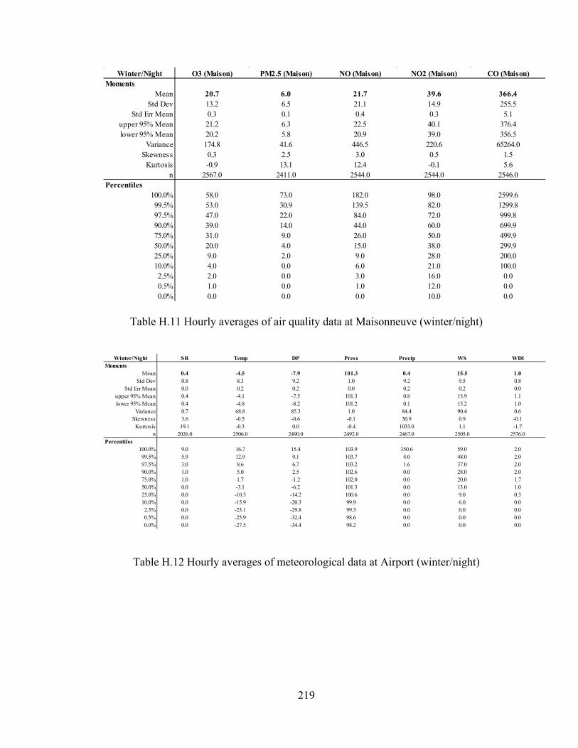
219
Table H.11 Hourly averages of air quality data at Maisonneuve (winter/night)
Table H.12 Hourly averages of meteorological data at Airport (winter/night)
Winter/Night O3 (Maison) PM2.5 (Maison) NO (Maison) NO2 (Maison) CO (Maison)Moments
Mean 20.7 6.0 21.7 39.6 366.4Std Dev 13.2 6.5 21.1 14.9 255.5
Std Err Mean 0.3 0.1 0.4 0.3 5.1upper 95% Mean 21.2 6.3 22.5 40.1 376.4lower 95% Mean 20.2 5.8 20.9 39.0 356.5
Variance 174.8 41.6 446.5 220.6 65264.0Skewness 0.3 2.5 3.0 0.5 1.5
Kurtosis -0.9 13.1 12.4 -0.1 5.6n 2567.0 2411.0 2544.0 2544.0 2546.0
Percentiles100.0% 58.0 73.0 182.0 98.0 2599.699.5% 53.0 30.9 139.5 82.0 1299.897.5% 47.0 22.0 84.0 72.0 999.890.0% 39.0 14.0 44.0 60.0 699.975.0% 31.0 9.0 26.0 50.0 499.950.0% 20.0 4.0 15.0 38.0 299.925.0% 9.0 2.0 9.0 28.0 200.010.0% 4.0 0.0 6.0 21.0 100.02.5% 2.0 0.0 3.0 16.0 0.00.5% 1.0 0.0 1.0 12.0 0.00.0% 0.0 0.0 0.0 10.0 0.0
Winter/Night SR Temp DP Press Precip WS WDIMoments
Mean 0.4 -4.5 -7.9 101.3 0.4 15.5 1.0Std Dev 0.8 8.3 9.2 1.0 9.2 9.5 0.8
Std Err Mean 0.0 0.2 0.2 0.0 0.2 0.2 0.0upper 95% Mean 0.4 -4.1 -7.5 101.3 0.8 15.9 1.1lower 95% Mean 0.4 -4.8 -8.2 101.2 0.1 15.2 1.0
Variance 0.7 68.8 85.3 1.0 84.4 90.4 0.6Skewness 3.6 -0.5 -0.6 -0.1 30.9 0.9 -0.1
Kurtosis 19.1 -0.3 0.0 -0.4 1033.0 1.1 -1.7n 2026.0 2506.0 2490.0 2492.0 2467.0 2505.0 2576.0
Percentiles100.0% 9.0 16.7 15.4 103.9 350.6 59.0 2.099.5% 5.9 12.9 9.1 103.7 4.0 48.0 2.097.5% 3.0 8.6 6.7 103.2 1.6 37.0 2.090.0% 1.0 5.0 2.5 102.6 0.0 28.0 2.075.0% 1.0 1.7 -1.2 102.0 0.0 20.0 1.750.0% 0.0 -3.1 -6.2 101.3 0.0 13.0 1.025.0% 0.0 -10.3 -14.2 100.6 0.0 9.0 0.310.0% 0.0 -15.9 -20.3 99.9 0.0 6.0 0.02.5% 0.0 -23.1 -29.8 99.3 0.0 0.0 0.00.5% 0.0 -25.9 -32.4 98.6 0.0 0.0 0.00.0% 0.0 -27.5 -34.4 98.2 0.0 0.0 0.0

220
Appendix I Sample Model Outputs For Case Study 1 (Day Period)
Table I.1 Model output MLR
Table I.2 Model output PCA
Response OP (Airport) Summer Day
Summary of FitR2 0.68R2 (Adj) 0.67RMSE 17.44Mean of Response 78.93Observations 506
Analysis of Variance DF SS MS F Ratio Prob > FModel 7 314801 44972 148 <.0001Error 498 151470 304C. Total 505 466272
Parameter Estimates Estimate Std Error t Ratio Prob>|t|Intercept -629.04 149.50 -4.21 <.0001PM2.5 (Airport) 1.84 0.13 14.52 <.0001NO (Airport) -1.66 0.23 -7.32 <.0001CO (Airport) 0.036 0.011 3.29 0.0011Temp 2.81 0.24 11.66 <.0001DP -2.90 0.29 -10.09 <.0001Press 6.50 1.49 4.37 <.0001WDI 4.53 1.09 4.13 <.0001
PC1 PC2 PC3 PC4 PC5 PC6 PC7 PC8 PC9 PC10 PC11Eigenvalue 2.97 2.09 1.39 1.05 0.90 0.81 0.53 0.49 0.34 0.30 0.12Percent 27.02 19.00 12.66 9.59 8.15 7.36 4.86 4.45 3.13 2.73 1.05Cum Percent 27.02 46.02 58.68 68.27 76.42 83.78 88.64 93.09 96.22 98.95 100.00PM2.5 (Airpo 0.45 0.17 -0.05 -0.19 0.19 0.15 0.09 -0.36 0.60 -0.41 -0.08NO (Airport) 0.18 -0.49 0.03 -0.22 -0.25 -0.12 0.32 0.60 0.13 -0.34 0.02NO2 (Airport 0.28 -0.50 0.05 -0.15 -0.01 0.00 0.16 -0.28 0.18 0.71 -0.02CO (Airport) 0.47 -0.16 -0.18 -0.06 0.06 0.07 0.08 -0.29 -0.70 -0.25 0.27SR 0.10 0.04 0.42 0.59 -0.56 0.07 0.25 -0.24 0.06 -0.10 0.10Temp 0.39 0.39 0.19 -0.04 0.05 0.15 -0.11 0.41 0.09 0.28 0.60DP 0.50 0.19 -0.04 0.20 -0.05 0.10 -0.12 0.29 -0.17 0.15 -0.71Press -0.12 0.15 0.62 -0.24 0.39 0.16 0.51 0.02 -0.23 0.01 -0.18Precip 0.03 -0.22 -0.16 0.66 0.63 -0.06 0.20 0.16 0.12 -0.03 0.10WS -0.18 0.16 -0.52 0.00 -0.17 0.61 0.49 0.07 0.01 0.14 0.02WDI 0.09 0.40 -0.25 -0.05 -0.08 -0.72 0.47 -0.05 -0.01 0.14 0.00

221
Table I.3 Model output PCR
Response OP (Airport) Summer Day
Summary of FitR2 0.68R2 (Adj) 0.67RMSE 17.47Mean of Response 78.93Observations 506
Analysis of Variance DF SS MS F Ratio Prob > FModel 9 314833 34981 115 <.0001Error 496 151439 305C. Total 505 466272
Parameter Estimates Estimate Std Error t Ratio Prob>|t|Intercept 78.93 0.78 101.61 <.0001Prin Comp 1 6.42 0.45 14.23 <.0001Prin Comp 2 10.96 0.54 20.38 <.0001Prin Comp 3 4.29 0.66 6.52 <.0001Prin Comp 4 -7.58 0.76 -10.01 <.0001Prin Comp 5 7.69 0.82 9.36 <.0001Prin Comp 8 -8.57 1.11 -7.71 <.0001Prin Comp 9 8.87 1.33 6.69 <.0001Prin Comp 10 -3.81 1.42 -2.69 0.0075Prin Comp 11 19.38 2.29 8.47 <.0001
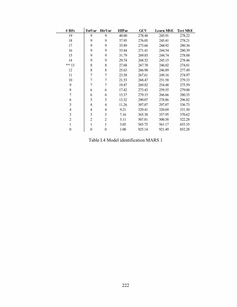
222
Table I.4 Model identification MARS 1
# BFs TotVar DirVar EffPar GCV Learn MSE Test MSE19 9 9 40.00 278.48 245.91 278.2218 9 9 37.95 276.05 245.41 278.2117 9 9 35.89 273.66 244.92 280.3616 9 9 33.84 271.41 244.54 280.3915 9 9 31.79 269.85 244.74 278.8814 9 9 29.74 268.52 245.15 278.46
** 13 8 8 27.68 267.70 246.02 274.8112 8 8 25.63 266.90 246.89 277.4911 7 7 23.58 267.61 249.16 274.9710 7 7 21.53 268.47 251.58 279.339 7 7 19.47 269.82 254.48 275.598 6 6 17.42 273.43 259.55 279.007 6 6 15.37 279.15 266.66 280.356 5 5 13.32 290.07 278.86 296.825 4 4 11.26 307.07 297.07 336.734 4 4 9.21 329.41 320.69 331.503 3 3 7.16 365.38 357.95 370.622 2 2 5.11 507.81 500.58 522.281 1 1 3.05 565.75 561.17 655.350 0 0 1.00 925.14 921.49 852.28

223
Table I.5 Model output MARS 1
Response OP (Airport) Summer Day
Summary of FitR2 0.74R2 (Adj) 0.73RMSE 15.68Mean of Response 78.93Observations 506
Analysis of Variance DF SS MS F Ratio Prob > FModel 13 345231 26556 108 <.0001Error 492 121041 246C. Total 505 466272
Parameter Estimates Estimate Std Error t Ratio Prob>|t|Constant 107.34 5.40 19.86 <.0001BF2 -2.64 0.16 -16.25 <.0001BF4 -3.48 0.73 -4.76 <.0001BF5 6.90 1.56 4.42 <.0001BF6 22.42 8.72 2.57 0.0104BF8 2.74 0.42 6.50 <.0001B11 -3.12 0.47 -6.64 <.0001BF12 2.73 0.31 8.92 <.0001BF14 -2.57 0.23 -11.35 <.0001BF15 20.96 6.53 3.21 0.0014BF16 -2.87 1.24 -2.31 0.0212BF17 -1.33 0.35 -3.80 0.0002BF19 0.00 0.00 -1.66 0.0981BF20 -0.23 0.09 -2.65 0.0083
BF2 = max ( 0 , 24 - PM2.5 (AIRPORT))
BF19 = max ( 0, SR - 85.00)
BF12 = max ( 0, 13.80 - DP) BF14 = max ( 0, 28.40 - TEMP) BF15 = max ( 0, WDI - 1.71) BF16 = max ( 0, 1.71 - WDI) BF17 = max ( 0, NO2 (AIRPORT) - 24.00)
BF11 = max( 0, DP - 13.80) BF8 = max ( 0, 11.00 - NO (AIRPORT)) BF6 = max ( 0, 99.69 - PRESS) BF5 = max ( 0, PRESS - 99.69) BF4 = max( 0, 6 - NO2 (AIRPORT))
BF20 = max ( 0, 85 - SR)

224
Table I.6 Model identification MARS 2
# BFs TotVar DirVar EffPar GCV Learn MSE Test MSE20 7 7 54.00 275.73 229.54 310.3919 7 7 51.35 272.55 229.09 312.9518 7 7 48.70 269.47 228.68 312.2517 7 7 46.05 266.83 228.60 313.4216 7 7 43.40 264.40 228.67 314.7115 7 7 40.75 263.55 230.09 320.5714 7 7 38.10 263.13 231.87 319.5213 7 7 35.45 264.57 235.31 307.8412 7 7 32.80 266.76 239.45 301.5411 7 7 30.15 271.64 246.07 300.45
**10 7 7 27.50 277.20 253.40 295.579 7 7 24.85 284.71 262.62 299.588 6 6 22.20 292.77 272.49 316.687 5 5 19.55 299.68 281.42 320.446 4 4 16.90 317.61 300.91 358.465 4 4 14.25 322.79 308.53 371.094 4 4 11.60 362.97 349.98 419.573 4 4 8.95 426.75 415.07 525.532 3 3 6.30 463.77 454.99 595.381 1 1 3.65 567.10 561.17 655.350 0 0 1.00 925.14 921.49 852.28

225
Table I.7 Model output MARS 2
Response OP (Airport) Summer Day
Summary of FitR2 0.73R2 (Adj) 0.73RMSE 15.91Mean of Response 78.93Observations 506
Analysis of Variance DF SS MS F Ratio Prob > FModel 10 340838 34084 135 <.0001Error 495 125434 253C. Total 505 466272
Parameter Estimates Estimate Std Error t Ratio Prob>|t|Constant 95.41 4.36 21.88 <.0001BF2 -1.87 0.17 -11.29 <.0001BF$ -4.65 0.74 -6.25 <.0001BF5 7.82 1.50 5.22 <.0001BF7 0.21 0.02 9.53 <.0001BF9 -0.28 0.02 -11.77 <.0001BF10 -0.92 0.21 -4.36 <.0001BF12 4.06 0.77 5.29 <.0001BF13 4.72 1.02 4.63 <.0001BF18 -0.06 0.01 -5.52 <.0001BF20 2.63 0.45 5.88 <.0001
BF2 = max ( 0, 24.00 - PM2.5 (AIRPORT)) BF3 = max ( 0, NO2 (AIRPORT) - 6.00) BF4 = max ( 0, 6.00 - NO2 (AIRPORT)) BF5 = max ( 0, PRESS - 99.69) BF7 = max ( 0, TEMP - 12.80) * BF3 BF9 = max ( 0, DP - 6.40) * BF3 BF10 = max ( 0, 6.40 - DP) * BF3 BF12 = max ( 0, 3.99 - NO (AIRPORT)) BF13 = max ( 0, WDI + 0.01) BF18 = max ( 0, 30.30 - TEMP) * BF2 BF20 = max ( 0, 9.40 - DP)

226
Table I.8 Model identification ANN
Table I.9 Model output ANN
Hidden Nodes R2 SSE R2 SSE1 0.70 139299 0.54 1935652 0.77 108684 0.56 185535
**3 0.80 91626 0.58 1780594 0.82 84669 0.57 1825725 0.84 73998 0.54 1926906 0.86 67053 0.49 2136017 0.87 62547 0.51 2066408 0.87 58456 0.51 2063149 0.90 47335 0.54 19583810 0.90 45519 0.55 189983
Train Test
Hidden Node Multiplier Constant PM2.5 (Airport) NO (Airport) NO2 (Airport) CO (Airport)1 -1.89 -12.05 -0.10 0.48 -0.06 0.002 0.75 1644.35 3.11 -0.89 1.44 -0.073 3.79 -48.48 0.02 0.01 -0.04 0.00
Hidden Node SR Temp DP Press Precip WS WDI1 0.00 0.05 -0.09 0.18 -0.35 0.03 -1.802 -0.01 0.48 -1.27 -15.92 -4.60 -0.75 -15.343 0.00 0.14 -0.20 0.49 -0.07 0.00 -0.13

227
Table I.10 Model identification PC-ANN
Table I.11 Model output PC-ANN
Hidden Nodes R2 SSE R2 SSE1 0.70 139299 0.54 1935392 0.77 108923 0.56 1846483 0.80 91988 0.57 1807264 0.83 80759 0.60 1710825 0.84 74892 0.55 1906816 0.86 67038 0.56 184314
**7 0.86 63908 0.67 1410348 0.88 54770 0.51 2077959 0.90 47915 0.50 21027110 0.90 45247 0.64 153146
Train Test
Hidden Node Multiplier Constant PC1 PC2 PC3 PC4 PC5 PC6 PC7 PC8 PC9 PC10 PC111 -3.41 -1.09 -0.29 -0.53 -0.53 -0.54 -0.76 -0.23 0.33 -0.92 0.27 -0.44 -1.702 -0.76 8.06 0.18 -2.85 2.79 1.23 -0.29 11.16 -5.55 2.22 -2.44 -4.70 -9.363 0.62 0.62 3.45 -6.86 -2.78 15.07 12.48 0.28 8.41 11.27 -1.27 -3.52 1.044 -2.96 0.28 -0.13 0.04 0.24 0.87 0.97 -0.08 -0.80 1.13 -1.08 2.20 0.895 0.87 4.67 -5.66 3.85 0.78 -5.55 2.95 -4.59 5.87 -2.23 -1.81 -1.72 4.966 0.83 -2.00 0.47 2.26 1.32 2.24 2.54 -0.25 -8.01 -3.51 -7.75 13.11 -2.677 1.31 -0.07 0.32 0.62 0.12 -1.54 0.82 1.62 -2.63 -3.83 2.68 1.96 0.53

228
Table I.12 Model identification PC*-ANN
Table I.13 Model output PC*-ANN
Hidden Nodes R2 SSE R2 SSE1 0.54 212917 0.46 2285982 0.61 183478 0.53 198867
**3 0.64 168788 0.55 1886014 0.67 155358 0.52 2029415 0.68 151507 0.47 2239586 0.70 140717 0.50 2110977 0.71 137117 0.50 2119888 0.71 133552 0.45 2326869 0.73 124098 0.41 25034710 0.73 123792 0.45 231049
Train Test
Hidden Node Multiplier Constant PC1 PC2 PC3 PC41 3.16 1.42 -0.42 -2.12 0.38 -0.43854722 -2.77 1.55 -1.06 -1.41 0.44 -0.56041443 -8.21 0.75 -0.06 -0.35 -0.10 0.235713

229
Appendix J Sample Error Diagnostics For Case Study 1 (Day Period)
Figure J.1 Residual Moments (MLR, PCR)

230
Figure J.2 Plot O3 observed by O3 predicted (MLR) in μg/m3
Figure J.3 Plot Residual by O3 predicted (MLR) in μg/m3
R² = 0.4814
0
20
40
60
80
100
120
140
160
0.0 20.0 40.0 60.0 80.0 100.0 120.0 140.0 160.0
MLR Linear (MLR)
-140.0
-120.0
-100.0
-80.0
-60.0
-40.0
-20.0
0.0
20.0
40.0
60.0
80.0
100.0
120.0
140.0
0.0 20.0 40.0 60.0 80.0 100.0 120.0 140.0 160.0
MLR

231
Figure J.4 Plot O3 observed by O3 predicted (PCR) in μg/m3
Figure J.5 Plot Residual by O3 predicted (PCR) in μg/m3
R² = 0.4802
0
20
40
60
80
100
120
140
160
0.0 20.0 40.0 60.0 80.0 100.0 120.0 140.0 160.0
PCR Linear (PCR)
-140.0
-120.0
-100.0
-80.0
-60.0
-40.0
-20.0
0.0
20.0
40.0
60.0
80.0
100.0
120.0
140.0
0.0 20.0 40.0 60.0 80.0 100.0 120.0 140.0 160.0
PCR

232
Figure J.6 Residual Moments (MARS 1, MARS 2)

233
Figure J.7 Plot O3 observed by O3 predicted (MARS 1) in μg/m3
Figure J.8 Plot Residual by O3 predicted (MARS 1) in μg/m3
R² = 0.6796
0
20
40
60
80
100
120
140
160
0.0 20.0 40.0 60.0 80.0 100.0 120.0 140.0 160.0
MARS 1 Linear (MARS 1)
-140.0
-120.0
-100.0
-80.0
-60.0
-40.0
-20.0
0.0
20.0
40.0
60.0
80.0
100.0
120.0
140.0
0.0 20.0 40.0 60.0 80.0 100.0 120.0 140.0 160.0
MARS 1

234
Figure J.9 Plot O3 observed by O3 predicted (MARS 2) in μg/m3
Figure J.10 Plot Residual by O3 predicted (MARS 2) in μg/m3
R² = 0.656
0
20
40
60
80
100
120
140
160
0.0 20.0 40.0 60.0 80.0 100.0 120.0 140.0 160.0
MARS 2 Linear (MARS 2)
-140.0
-120.0
-100.0
-80.0
-60.0
-40.0
-20.0
0.0
20.0
40.0
60.0
80.0
100.0
120.0
140.0
0.0 20.0 40.0 60.0 80.0 100.0 120.0 140.0 160.0
MARS 2

235
Figure J.11 Residual Moments (ANN, PC-ANN)

236
Figure J.12 Plot O3 observed by O3 predicted (ANN) in μg/m3
Figure J.13 Plot Residual by O3 predicted (ANN) in μg/m3
R² = 0.6026
0
20
40
60
80
100
120
140
160
0.0 20.0 40.0 60.0 80.0 100.0 120.0 140.0 160.0
ANN Linear (ANN)
-140.0
-120.0
-100.0
-80.0
-60.0
-40.0
-20.0
0.0
20.0
40.0
60.0
80.0
100.0
120.0
140.0
0.0 20.0 40.0 60.0 80.0 100.0 120.0 140.0 160.0
ANN

237
Figure J.14 Plot O3 observed by O3 predicted (PC-ANN) in μg/m3
Figure J.15 Plot Residual by O3 predicted (PC-ANN) in μg/m3
R² = 0.6842
0
20
40
60
80
100
120
140
160
0 20 40 60 80 100 120 140 160
PC - ANN Linear (PC - ANN)
-140.0
-120.0
-100.0
-80.0
-60.0
-40.0
-20.0
0.0
20.0
40.0
60.0
80.0
100.0
120.0
140.0
0.0 20.0 40.0 60.0 80.0 100.0 120.0 140.0 160.0
PC - ANN

238
Figure J.16 Residual Moments (PC*-ANN)

239
Figure J.17 Plot O3 observed by O3 predicted (PC*-ANN) in μg/m3
Figure J.18 Plot Residual by O3 predicted (PC*-ANN) in μg/m3
R² = 0.5609
0
20
40
60
80
100
120
140
160
0 20 40 60 80 100 120 140 160
PC* - ANN Linear (PC* - ANN)
-140.0
-120.0
-100.0
-80.0
-60.0
-40.0
-20.0
0.0
20.0
40.0
60.0
80.0
100.0
120.0
140.0
0.0 20.0 40.0 60.0 80.0 100.0 120.0 140.0 160.0
PC* - ANN