Comparative Analysis of Statistical Tools To Identify Recruitment-Environment

Relationships and Forecast Recruitment Strength

Bernard A. Megrey

Yong-Woo Lee

S. Allen Macklin

National Oceanic and Atmospheric AdministrationNational Marine Fisheries ServiceAlaska Fisheries Science Center

Seattle, WA 98115 USA

Overview

• Background and motivation

• Mechanics of testing procedures

• Results of application of 3 statistical tools to 2 data sets

• Concluding remarks and observations

Why Forecast Recruitment?

• Understand important bio-physical factors controlling the recruitment processes

– The ultimate test of a model is its ability to predict

• Project future stock dynamics

• Evaluate management scenarios

• Provide reference points for fishery management

• Assist commercial fisheries decision making

The data we collect as it relates to recruitment variability and the factors that influence it probably will not change dramatically in the near future.

“We should endeavor to treat the data differently in a statistical sense.”

R.J.H Beverton 1989

What are the best statistical tools for estimating environment-recruitment relationships and forecasting future

recruitment states?

? ??

??

?

Problems in ForecastingThe complexity of recruitment forecasting often seems beyond the

capabilities of traditional statistical analysis paradigms because….

• Bio-physical relationships are inherently nonlinear• Often there are limitations in theoretical development or standard

models cannot deal with data pathologies• Inability to meet required assumptions• Time series of data are short• Lack of degrees of freedom• The need to partition already short time series into segments

representing identified regimes

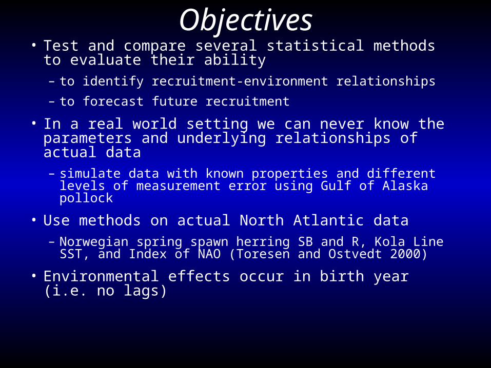
Objectives• Test and compare several statistical methods to evaluate

their ability– to identify recruitment-environment relationships

– to forecast future recruitment

• In a real world setting we can never know the parameters and underlying relationships of actual data– simulate data with known properties and different levels of

measurement error using Gulf of Alaska pollock

• Use methods on actual North Atlantic data – Norwegian spring spawn herring SB and R, Kola Line SST, and

Index of NAO (Toresen and Ostvedt 2000)

• Environmental effects occur in birth year (i.e. no lags)

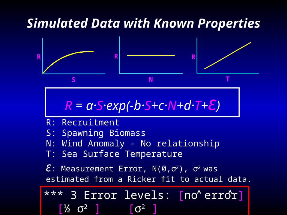
Simulated Data with Known Properties

R = a·S·exp(-b·S+c·N+d·T+ε)R: RecruitmentS: Spawning Biomass N: Wind Anomaly - No relationship T: Sea Surface Temperature

ε: Measurement Error, N(0,σ2), σ2 was estimated from a Ricker fit to actual data.

N

R

S

R

T

R

*** 3 Error levels: [no error] [½ σ2 ] [σ2 ]^ ^

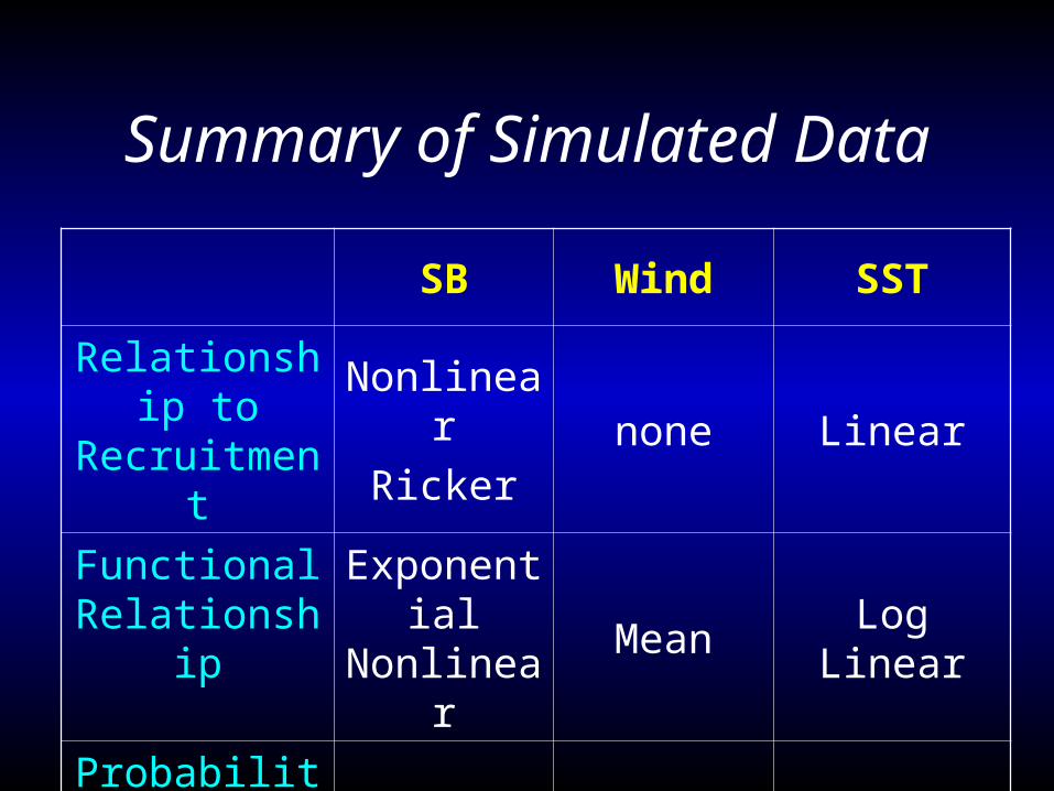
Summary of Simulated Data

SB Wind SST

Relationship to Recruitment

Nonlinear

Rickernone Linear

Functional Relationship

Exponential Nonlinear

Mean Log Linear

Probability

DistributionGamma Lognormal Normal

0 10 200

10

20

30

40

50

SB

R

2 3 4 50

10

20

30

40

50

SSTR

-5 0 50

10

20

30

40

50

NAO

R

0 0.5 10

1

2

3

4

SB

R

-10 -5 0 50

1

2

3

4

SST

R

0 1 2 30

1

2

3

4

Wind

R

Herring

Simulated

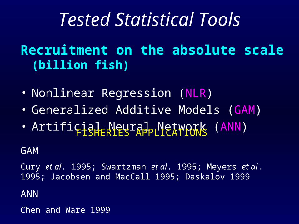
Tested Statistical Tools

Recruitment on the absolute scale (billion fish)

• Nonlinear Regression (NLR)• Generalized Additive Models (GAM)• Artificial Neural Network (ANN)

FISHERIES APPLICATIONS

GAM

Cury et al. 1995; Swartzman et al. 1995; Meyers et al. 1995; Jacobsen and MacCall 1995; Daskalov 1999

ANN

Chen and Ware 1999

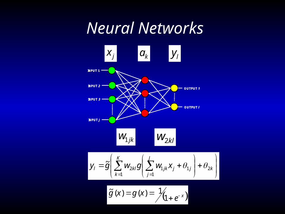
Neural Networks

INPUT 1

INPUT 2

INPUT 3

INPUT j

OUTPUT l

OUTPUT 1

INPUT 1

INPUT 2

INPUT 3

INPUT j

OUTPUT l

OUTPUT 1

jx ly

jkw1 klw2

kjj

J

jjk

K

kkll xwgwgy 21

11

12

~

xexgxg

1

1)()(~

ka

General Additive Models

)()(1

jj

p

j

Xfm

Comparisons

Statistical Methods• Parametric (NLR) vs. Non-parametric (GAM, ANN)• Conventional (NLR) vs. Innovative (GAM, ANN)• Model Free (GAM, ANN) vs. functional relationships specified a priori (NLR)

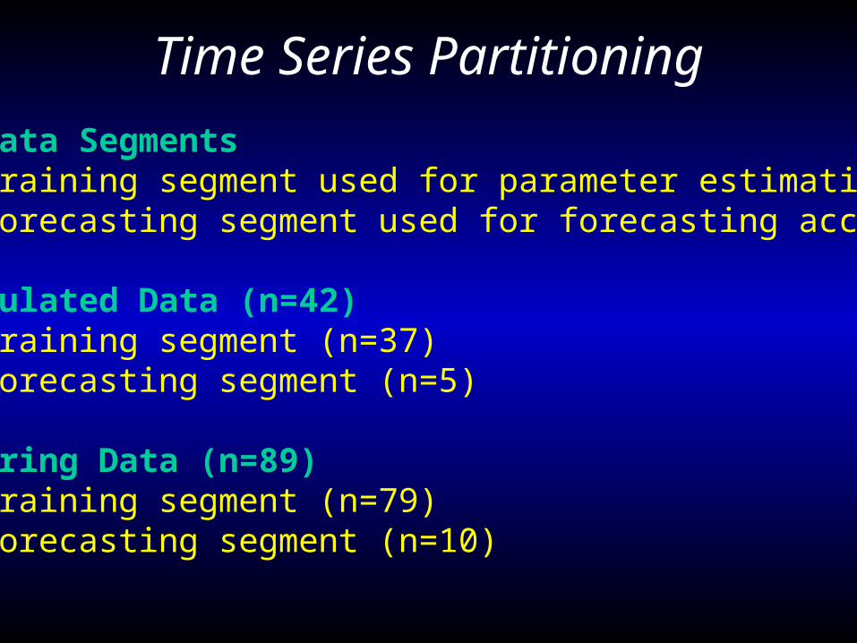
Time Series Partitioning

2 Data Segments• Training segment used for parameter estimation• Forecasting segment used for forecasting accuracy

Simulated Data (n=42)• Training segment (n=37)• Forecasting segment (n=5)

Herring Data (n=89)• Training segment (n=79)• Forecasting segment (n=10)

Simulated vs Predicted, for Error level = 0

0.0

0.5

1.0

1.5

2.0

2.5

3.0

3.5

4.0

1960 1965 1970 1975 1980 1985 1990 1995 2000

SIM

-1.0

-0.5

0.0

0.5

1.0

1.5

2.0

2.5

3.0

3.5

4.0

1960 1965 1970 1975 1980 1985 1990 1995 2000

SIM

GAM

NLR

ANN

-1.0

-0.5

0.0

0.5

1.0

1.5

2.0

2.5

3.0

3.5

4.0

1960 1965 1970 1975 1980 1985 1990 1995 2000

SIM

GAM

NLR

ANN

-1.0

-0.5

0.0

0.5

1.0

1.5

2.0

2.5

3.0

3.5

4.0

1960 1965 1970 1975 1980 1985 1990 1995 2000

SIM

GAM

NLR

ANN

R-square for Training

0.88

1.00

0.92

0.4

0.6

0.8

1.0

GAM NLR ANN

MSE for Forecasting

0.080.000.140.0

0.2

0.4

0.6

GAM NLR ANN

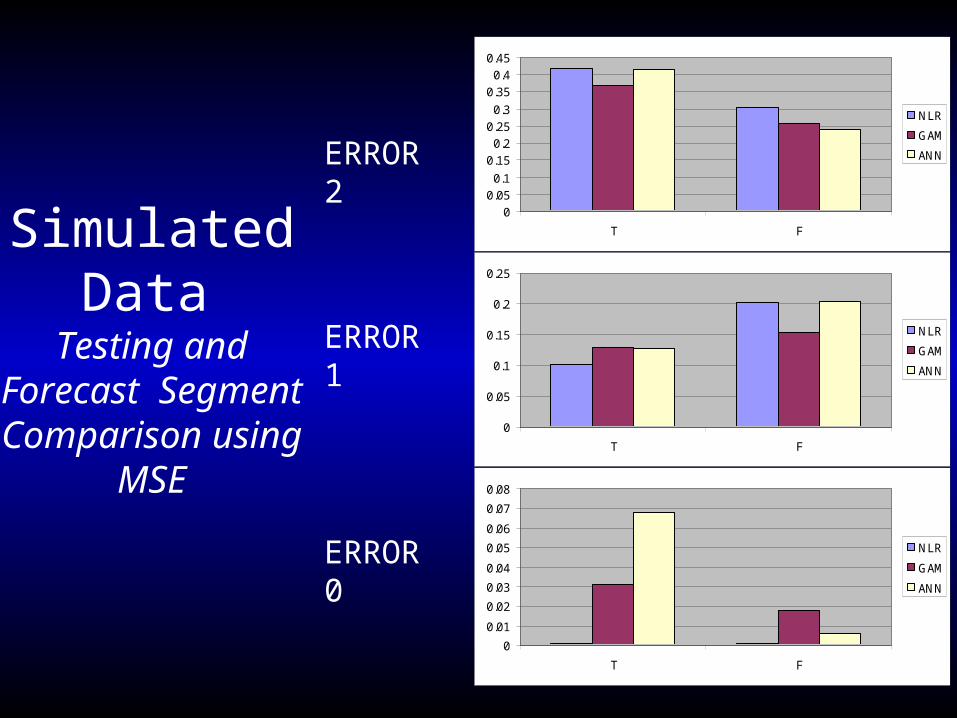
Simulated Data

Testing and Forecast SegmentComparison using

MSE

0

0.05

0.1

0.15

0.2

0.25

0.3

0.35

0.4

0.45

T F

NLR

GAM

ANN

0

0.05

0.1

0.15

0.2

0.25

T F

NLR

GAM

ANN

0

0.01

0.02

0.03

0.04

0.05

0.06

0.07

0.08

T F

NLR

GAM

ANN

ERROR 2

ERROR 1

ERROR 0

Simulated Data ANN

Relative WeightComparison

3 variables

2 hidden neurons

10 parms0

0.1

0.2

0.3

0.4

0.5

0.6

0.7

0.8

SB SST WIND

ERR0

ERR1

ERR2

0

0.1

0.2

0.3

0.4

0.5

0.6

0.7

0.8

SB SST

ERR0

ERR1

ERR2

2 variables

2 hidden neurons

8 parms

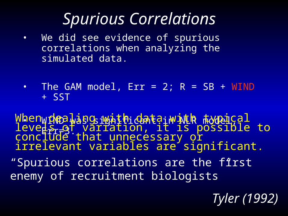
Spurious Correlations• We did see evidence of spurious correlations when

analyzing the simulated data.

• The GAM model, Err = 2; R = SB + WIND + SST

• WIND was significant in NLR model, Err=3.

When dealing with data with typical levels of variation, it is possible to conclude that unnecessary or irrelevant variables are significant.

“Spurious correlations are the first enemy of recruitment biologists”

Tyler (1992)

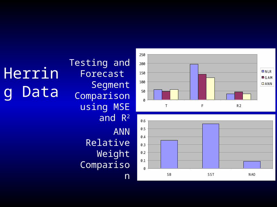
Herring Data

Testing and Forecast SegmentComparison using

MSE and R2

ANN Relative Weight

Comparison0

0.1

0.2

0.3

0.4

0.5

0.6

SB SST NAO

0

50

100

150

200

250

T F R2

NLR

GAM

ANN

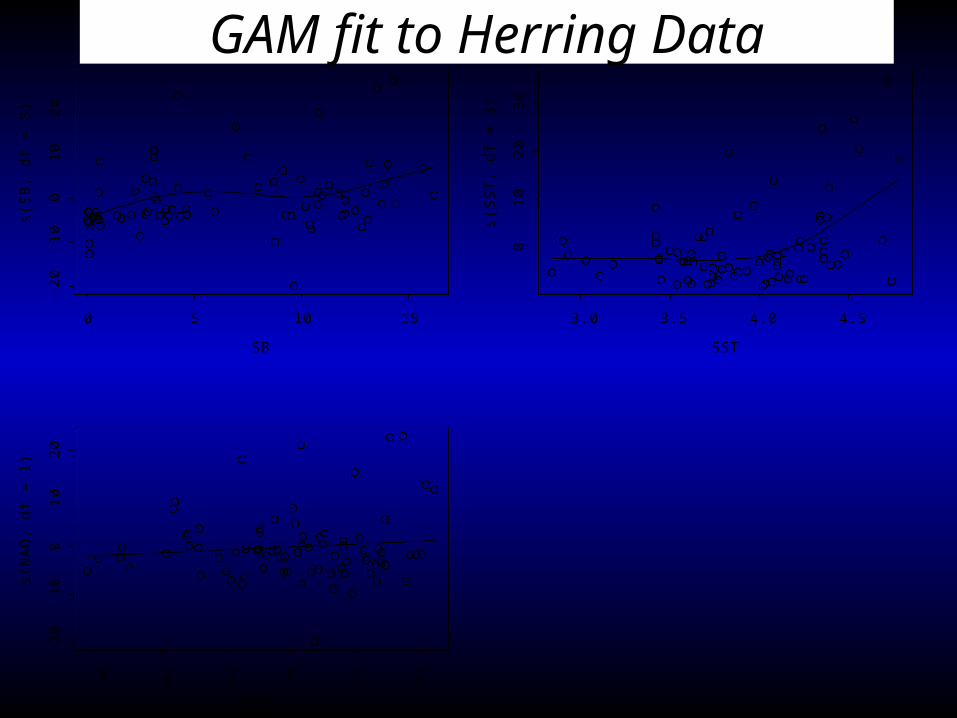
SB

s(S

B, d

f = 3

)

0 5 10 15

-20

-10

01

02

0

SST

s(S

ST,

df =

3)

3.0 3.5 4.0 4.5

01

02

03

0

NAO

s(N

AO

, df =

1)

-3 -2 -1 0 1 2

-20

-10

01

02

0GAM fit to Herring Data

Summary• Need to be cautious when dealing with noisy data,

because a wrong model or variable could be identified as influential to recruitment.

• We did see evidence of spurious correlations under very controlled data situations.

• It appears that ANNs forecast better than conventional parametric methods when data are noisy.

• Non-parametric methods (GAMs and ANNs) work well for suggesting functional relationships and forecasting future recruitment states– desirable property because real systems are highly non-

linear and include complex interactions among the variables.

Summary (con’t)• There is no one “best” method to address the environment-

recruitment problem.

• ANNs are highly flexible and show promise for forecasting, thus using GAMs and ANNs together with more traditional methods should enhance analysis and forecasting.

• When considering estimation in conjunction with forecasting it is better to consider a balance between “best” models.

• Results underscore the need to build good conceptual models first, then guided by hypotheses regarding factors that control recruitment and their time and space scales of influence, judiciously apply a suite of statistical models to quality data sets.

• Data mining and “kitchen stew” correlation exercises are not appropriate.