comparing lbp, hog and deep features for classiﬁcation of ... · we use kimia path960, a publicly...

Comparing LBP, HOG and Deep Featuresfor Classification of Histopathology Images

Taha J. Alhindi1,2,3, Shivam Kalra∗1,3, Ka Hin Ng3, Anika Afrin4, Hamid R. Tizhoosh1

1 Kimia Lab, University of Waterloo, Canada2 Dept. of Industrial Eng., King Abdulaziz Univ., Jeddah, Saudi Arabia

3 Systems Design Engineering, University of Waterloo, Canada4 Electrical and Computer Engineering, University of Waterloo, Canada{shivam.kalra, talhindi, kh7ng, aafrin, tizhoosh}@uwaterloo.ca

Abstract— Medical image analysis has become a topic underthe spotlight in recent years. There is a significant progressin medical image research concerning the usage of machinelearning. However, there are still numerous questions andproblems awaiting answers and solutions, respectively. In thepresent study, comparison of three classification models isconducted using features extracted using local binary patterns,the histogram of gradients, and a pre-trained deep network.Three common image classification methods, including supportvector machines, decision trees, and artificial neural networksare used to classify feature vectors obtained by different featureextractors. We use KIMIA Path960, a publicly available datasetof 960 histopathology images extracted from 20 different tissuescans to test the accuracy of classification and feature extrac-tions models used in the study, specifically for the histopathologyimages. SVM achieves the highest accuracy of 90.52% usinglocal binary patterns as features which surpasses the accuracyobtained by deep features, namely 81.14%.

I. INTRODUCTION

IN recent years, machine learning has become a populartopic and its applications are increasing day by day with

respect to image-based diagnosis, disease prediction and riskassessment [1]. Machine learning is considered a sub-area ofartificial intelligence, a set of methods which learn from pastdata to generalize to new data, can handle noisy input andcomplex data environments, use prior knowledge, and canform new concepts [2].

After recent success of machine learning, and speciallydeep learning, in various application fields, some approachesare providing solutions with good accuracy for medicalimaging making it a great opportunity for future applicationsin the healthcare sector. Major experimentation attemptsfor computer-aided diagnosis had begun in the mid-1980swhen the primary focus was on the techniques for detect-ing lesions on chest radiographs and mammograms [3]. Inrecent years, machine-learning approaches are being usedsuccessfully in the area of image-based disease detection andforecasting. Oliver et al. proposed an approach for reducingfalse positives for recognition of mammography images usinglocal binary pattern (LBP) in 2007 [4]. LBP was used for

∗Shivam Kalra is a corresponding author for the research work.

extracting the descriptors and detected masses were classifiedinto either malignant or benign with support vector machines(SVM). The result of the experiment showed that the LBPfeatures were successful in not only in terms of false positivereduction but also it was efficient compared to other methodsfor diverse mass areas, which is an acute feature of thesystems for mass detection. An appraisal of bag-of-featuresapproach for classifying histopathology images had beenproposed by Caicedo et al. in 2009 [5]. The key advantage oftheir proposed framework is that it is focusing to the contentsof the image group particularly. This property is achieved byan automated codebook construction and the visual featuredescriptors.

An image analysis methodology using SVM classifier todifferentiate low and high grades of breast cancer auto-matically has been proposed by Doyle et al. in 2008 [6].The dataset contained 48 breast biopsy tissue images havingover 3400 image features. After the feature dimensionalityreduction and SVM classification, the system achieved anaccuracy of 95.8% in differentiating cancerous from non-cancerous cases where Gabor filter features had been used.Distinguishing high-level from low-level cancer was donewith architectural features and an accuracy of 93.3% wasachieved. Moreover, they used spectral clustering to visualizethe hidden manifold form which consists various grades ofcancer, and it showed a steady shift from low-grade to high-grade breast cancer.

Kumar et al. conducted a recent study which comparesdeep features, bag-of-visual-words (BoVW) and LBP forthe classification of histopathology image dataset, KIMIAPath960. The classification accuracy obtained in the studyusing LBP and deep features were 90.62% and 94.72%,respectively, whereas BoVW achieved the highest accuracyof 96.50% [7].

In the present study, comparison of three classificationmodels is conducted. The dataset used is KIMIA Path960 [7].The models use one of the following feature extractors: Localbinary pattern (LBP), histogram of gradients (HOG) anddeep features from VGG 19, a pre-trained deep network.The feature vectors are then provided as an input to train

arX

iv:1

805.

0583

7v1

[ee

ss.I

V]

3 M

ay 2

018

Accepted for publication in proceedings of the IEEE World Congress on Computational Intelligence (IEEE WCCI), Rio de Janeiro, Brazil, 8-3 July, 2018

several classifiers, for this paper, SVM, decision trees (DTs),and Artificial Neural Networks (ANNs, which use a shallowmulti-layer-perceptron) have been selected. The study willempirically justify applications of various feature extractionmodels and classification methods that are commonly avail-able for the histopathology image analysis.

The study is divided into 5 sections, where feature extrac-tors and classification algorithms are discussed in Section II.The dataset is introduced in Section III. Section IV explainsthe methodology used in the study. Experiments and resultsare discussed in Section IV later. Conclusions are drawn inSection V.

II. BACKGROUND

A. Feature Extractors

Local Binary Pattern (LBP): LBP was introduced in1994 [8]. Yet, the texture spectrum model of LBP wasproposed even earlier in 1990 [9]. LBP feature extractorhas been applied in many areas after Ojala and Pietikainen’sresearch in multi-resolution approach in 2002 [10], includingtext identification [11] and face recognition [5]. Wang hascombined LBP with Histogram of Oriented Gradients (HOG)descriptor to improve detection performance in [12].

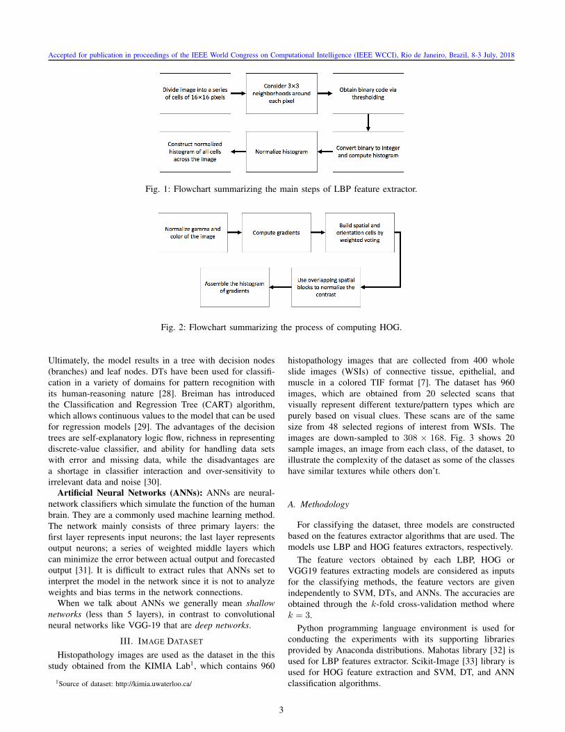
Classical LBP feature extractor should follow specificactions; these actions are summarized in Fig. 1 [7].

There are series of attempts to improve the LBP method.One recent version finds the intensity values of points in acircular neighborhood by considering the values which havesmall circular neighborhoods around the central pixel [13].

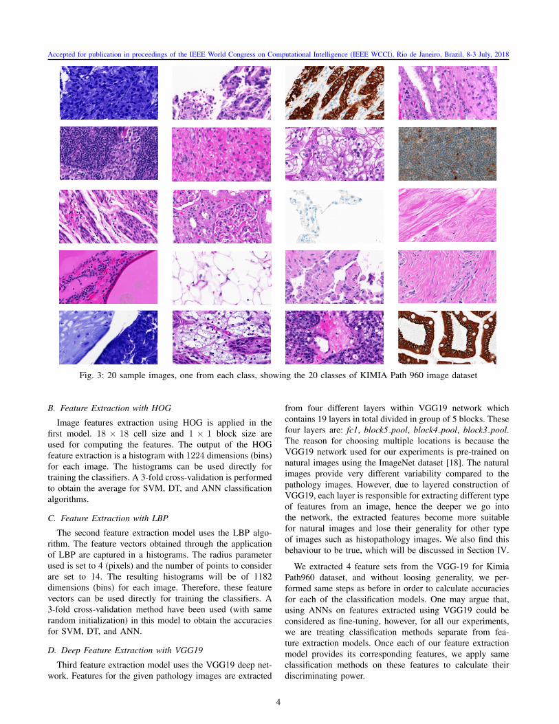
Histogram of Oriented Gradients (HOG): HOG cap-tures features by counting the occurrence of gradient ori-entation. Traditional HOG divides the image into differentcells and computes a histogram of gradient orientationsover them [13]. HOG is being applied extensively in objectrecognition areas as facial recognition[14]. The process forcomputing HOG is explained in Fig. 2 [15].

VGG:A Pre-Trained Deep Net: VGG 16 and 19 are deepconvolutional networks (ConvNet) architecture first proposedby K. Simonyan and A. Zisserman from Visual GeometryGroup of University of Oxford in 2014 [16]. In the paper,an evaluation of very-deep networks for large-scale imageclassification was carried out: the generic architecture ofthe network contained a very small convolution filter withsmall receptive field of 3 × 3 and the convolutional pacewas fixed to 1 pixel, while five max-pooling layers carriedout the spatial pooling, over a 2 × 2 pixel window, with aconvolution step of 2 [16]. There were three fully-connectedlayers of same configuration: the first and second layers had4096 channels each, whereas, the third layer contained 1000channels and performed ILSVRC-2012 dataset classifica-tion [16]. The ConvNet configurations analyzed in this studyfollowed the same architecture which only differ in depth:from network A to E where the depths differ from weightlayer 11 to 19 [16]. The results of classification experimentsin single-scale, multi-scale and multi-crop evaluation shownthat a major improvement could be achieved in this proposed

network if the depth was pushed to 16 and to 19 weightlayers, which were VGG16 and VGG19 [16].

In recent years, deep learning has been widely used inmedical sector in terms of automated cancer and lesiondetection. In 2015, Ertosun and Rubin developed a searchsystem basing on deep learning to automatically search andlocalize masses, where the system contained a classificationand a localization engine as well [17]. There are alsoworks applying deep convolution neural network classifiersto mammograms such as AlexNet [18], VGG net [16] andGoogLeNet [19].

Another study on finding breast cancer from lymph nodebiopsy images has been carried out by Wang, Dayong, etal. [20] in 2016 using deep learning classification mod-els, including GoogLeNet, VGG-16, AlexNet and FaceNet.Combining estimation from deep learning systems with thediagnosis of the human pathologist, the pathologist’s areaunder the receiver operating curve (AUC) was increased to0.995, representing nearly 85% reduction in human errorrate [20], which means that integration of deep learningapproaches with the workflow of pathologists could increasethe accuracy in cancer diagnosis.

Radon Features: Although we do not experiment withthem in this study, we have to mention several approachesthat have been proposed to use Radon transform for featureextraction [21], [22]. These methods use projections in localneighbourhood to assemble a feature vector or a histogram.The most recent work reports retrieval accuracies usingencoded local projections, short ELP histogram, that surpassdeep features for histopathology images [22].

B. Classifiers

Support Vector Machines (SVM): SVM is a classifierdesigned for binary problems with extension to multi-classproblems [23]. Cortes and Vapnik firstly introduced SVMin 1995, with the main idea to ensure the network’s highgeneralization ability by mapping inputs non-linearly to high-dimensional feature spaces, where linear decision surfaceswere constructed with special properties [24]. The originalidea of support vector network was implied for the situationthat training data was separable by a hyperplane withouterror. Later, Cortes and Vapnik introduced the notion of soft-margins such that a minimal subset of error in the trainingdata is permit table, allowing the remaining part of thetraining data to be separated by constructing an optimalseparating hyperplane [24]. Some advantages of the SVMare the generalization of binary and regression forms andnotation simplification [23]. SVM uses several kernels suchas the polynomial kernel, linear kernel, and the gaussianradial basis function (RBF) kernel [25], [26].

Decision Trees: Decision Trees (DTs) are classifiers rep-resented by a flowchart-like tree structure introduced by J.R. Quinlan in 1986 [27]. DTs do neither make any statisticalassumption concerning the inputs nor involve scaling of thedata, dissimilar to SVM and neural networks. DT modelsare constructed in terms of a tree structure in which thedataset is broken down into smaller subsets at each branch.

2


Fig. 1: Flowchart summarizing the main steps of LBP feature extractor.

Fig. 2: Flowchart summarizing the process of computing HOG.

Ultimately, the model results in a tree with decision nodes(branches) and leaf nodes. DTs have been used for classifi-cation in a variety of domains for pattern recognition withits human-reasoning nature [28]. Breiman has introducedthe Classification and Regression Tree (CART) algorithm,which allows continuous values to the model that can be usedfor regression models [29]. The advantages of the decisiontrees are self-explanatory logic flow, richness in representingdiscrete-value classifier, and ability for handling data setswith error and missing data, while the disadvantages area shortage in classifier interaction and over-sensitivity toirrelevant data and noise [30].

Artificial Neural Networks (ANNs): ANNs are neural-network classifiers which simulate the function of the humanbrain. They are a commonly used machine learning method.The network mainly consists of three primary layers: thefirst layer represents input neurons; the last layer representsoutput neurons; a series of weighted middle layers whichcan minimize the error between actual output and forecastedoutput [31]. It is difficult to extract rules that ANNs set tointerpret the model in the network since it is not to analyzeweights and bias terms in the network connections.

When we talk about ANNs we generally mean shallownetworks (less than 5 layers), in contrast to convolutionalneural networks like VGG-19 that are deep networks.

III. IMAGE DATASET

Histopathology images are used as the dataset in the thisstudy obtained from the KIMIA Lab1, which contains 960

1Source of dataset: http://kimia.uwaterloo.ca/

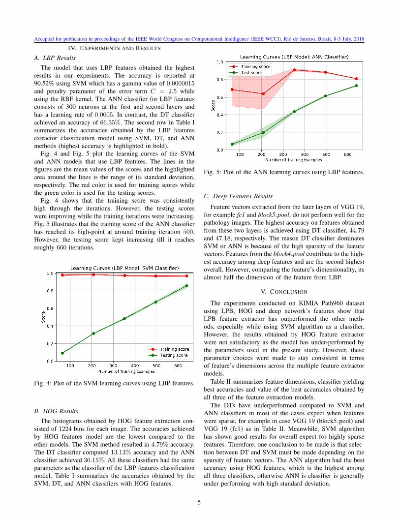
histopathology images that are collected from 400 wholeslide images (WSIs) of connective tissue, epithelial, andmuscle in a colored TIF format [7]. The dataset has 960images, which are obtained from 20 selected scans thatvisually represent different texture/pattern types which arepurely based on visual clues. These scans are of the samesize from 48 selected regions of interest from WSIs. Theimages are down-sampled to 308 × 168. Fig. 3 shows 20sample images, an image from each class, of the dataset, toillustrate the complexity of the dataset as some of the classeshave similar textures while others don’t.

A. Methodology

For classifying the dataset, three models are constructedbased on the features extractor algorithms that are used. Themodels use LBP and HOG features extractors, respectively.

The feature vectors obtained by each LBP, HOG orVGG19 features extracting models are considered as inputsfor the classifying methods, the feature vectors are givenindependently to SVM, DTs, and ANNs. The accuracies areobtained through the k-fold cross-validation method wherek = 3.

Python programming language environment is used forconducting the experiments with its supporting librariesprovided by Anaconda distributions. Mahotas library [32] isused for LBP features extractor. Scikit-Image [33] library isused for HOG feature extraction and SVM, DT, and ANNclassification algorithms.

3

http://kimia.uwaterloo.ca/


Fig. 3: 20 sample images, one from each class, showing the 20 classes of KIMIA Path 960 image dataset

B. Feature Extraction with HOG

Image features extraction using HOG is applied in thefirst model. 18 × 18 cell size and 1 × 1 block size areused for computing the features. The output of the HOGfeature extraction is a histogram with 1224 dimensions (bins)for each image. The histograms can be used directly fortraining the classifiers. A 3-fold cross-validation is performedto obtain the average for SVM, DT, and ANN classificationalgorithms.

C. Feature Extraction with LBP

The second feature extraction model uses the LBP algo-rithm. The feature vectors obtained through the applicationof LBP are captured in a histograms. The radius parameterused is set to 4 (pixels) and the number of points to considerare set to 14. The resulting histograms will be of 1182dimensions (bins) for each image. Therefore, these featurevectors can be used directly for training the classifiers. A3-fold cross-validation method have been used (with samerandom initialization) in this model to obtain the accuraciesfor SVM, DT, and ANN.

D. Deep Feature Extraction with VGG19

Third feature extraction model uses the VGG19 deep net-work. Features for the given pathology images are extracted

from four different layers within VGG19 network whichcontains 19 layers in total divided in group of 5 blocks. Thesefour layers are: fc1, block5 pool, block4 pool, block3 pool.The reason for choosing multiple locations is because theVGG19 network used for our experiments is pre-trained onnatural images using the ImageNet dataset [18]. The naturalimages provide very different variability compared to thepathology images. However, due to layered construction ofVGG19, each layer is responsible for extracting different typeof features from an image, hence the deeper we go intothe network, the extracted features become more suitablefor natural images and lose their generality for other typeof images such as histopathology images. We also find thisbehaviour to be true, which will be discussed in Section IV.

We extracted 4 feature sets from the VGG-19 for KimiaPath960 dataset, and without loosing generality, we per-formed same steps as before in order to calculate accuraciesfor each of the classification models. One may argue that,using ANNs on features extracted using VGG19 could beconsidered as fine-tuning, however, for all our experiments,we are treating classification methods separate from fea-ture extraction models. Once each of our feature extractionmodel provides its corresponding features, we apply sameclassification methods on these features to calculate theirdiscriminating power.

4


IV. EXPERIMENTS AND RESULTS

A. LBP Results

The model that uses LBP features obtained the highestresults in our experiments. The accuracy is reported at90.52% using SVM which has a gamma value of 0.0000015and penalty parameter of the error term C = 2.5 whileusing the RBF kernel. The ANN classifier for LBP featuresconsists of 300 neurons at the first and second layers andhas a learning rate of 0.0005. In contrast, the DT classifierachieved an accuracy of 66.35%. The second row in Table Isummarizes the accuracies obtained by the LBP featuresextractor classification model using SVM, DT, and ANNmethods (highest accuracy is highlighted in bold).

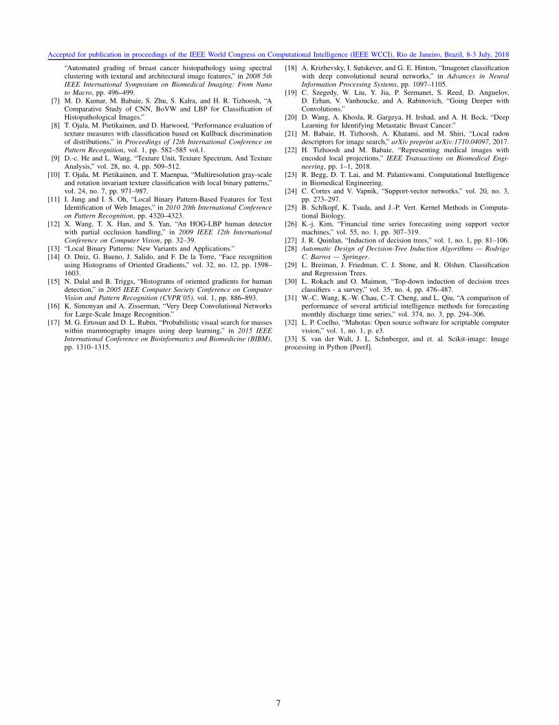
Fig. 4 and Fig. 5 plot the learning curves of the SVMand ANN models that use LBP features. The lines in thefigures are the mean values of the scores and the highlightedarea around the lines is the range of its standard deviation,respectively. The red color is used for training scores whilethe green color is used for the testing scores.

Fig. 4 shows that the training score was consistentlyhigh through the iterations. However, the testing scoreswere improving while the training iterations were increasing.Fig. 5 illustrates that the training score of the ANN classifierhas reached its high-point at around training iteration 500.However, the testing score kept increasing till it reachesroughly 660 iterations.

Fig. 4: Plot of the SVM learning curves using LBP features.

B. HOG Results

The histograms obtained by HOG feature extraction con-sisted of 1224 bins for each image. The accuracies achievedby HOG features model are the lowest compared to theother models. The SVM method resulted in 4.79% accuracy.The DT classifier computed 13.13% accuracy and the ANNclassifier achieved 36.15%. All these classifiers had the sameparameters as the classifier of the LBP features classificationmodel. Table I summarizes the accuracies obtained by theSVM, DT, and ANN classifiers with HOG features.

Fig. 5: Plot of the ANN learning curves using LBP features.

C. Deep Features Results

Feature vectors extracted from the later layers of VGG 19,for example fc1 and block5 pool, do not perform well for thepathology images. The highest accuracy on features obtainedfrom these two layers is achieved using DT classifier, 44.79and 47.18, respectively. The reason DT classifier dominatesSVM or ANN is because of the high sparsity of the featurevectors. Features from the block4 pool contribute to the high-est accuracy among deep features and are the second highestoverall. However, comparing the feature’s dimensionality, itsalmost half the dimension of the feature from LBP.

V. CONCLUSION

The experiments conducted on KIMIA Path960 datasetusing LPB, HOG and deep network’s features show thatLPB feature extractor has outperformed the other meth-ods, especially while using SVM algorithm as a classifier.However, the results obtained by HOG feature extractorwere not satisfactory as the model has under-performed bythe parameters used in the present study. However, theseparameter choices were made to stay consistent in termsof feature’s dimensions across the multiple feature extractormodels.

Table II summarizes feature dimensions, classifier yieldingbest accuracies and value of the best accuracies obtained byall three of the feature extraction models.

The DTs have underperformed compared to SVM andANN classifiers in most of the cases expect when featureswere sparse, for example in case VGG 19 (block5 pool) andVGG 19 (fc1) as in Table II. Meanwhile, SVM algorithmhas shown good results for overall expect for highly sparsefeatures. Therefore, one conclusion to be made is that selec-tion between DT and SVM must be made depending on thesparsity of feature vectors. The ANN algorithm had the bestaccuracy using HOG features, which is the highest amongall three classifiers, otherwise ANN is classifier is generallyunder performing with high standard deviation.

5


Feature ExtractionModels

Classification AlgorithmsSVM DT ANN

LBP

Fold 1 91.56% 65.31% 77.50%Fold 2 88.75% 66.25% 76.25%Fold 3 91.25% 67.50% 75.10%

All Folds 90.52± 1.26% 66.35± 0.90% 75.10± 2.56%

HOG

Fold 1 3.44% 11.25% 36.25%Fold 2 7.81% 13.44% 35.94%Fold 3 3.13% 14.69% 36.25%

All Folds 4.79± 2.14% 13.13± 1.42% 36.15± 0.15%

VGG19(fc1)

Fold 1 9.37% 45.31% 5.62%Fold 2 9.68% 45.93% 1.25%Fold 3 9.06% 43.12% 4.37%

All Folds 9.37± 0.25% 44.79± 1.2% 7.50± 1.83%

VGG19(block5 pool)

Fold 1 8.75% 48.75% 16.87%Fold 2 5.93% 47.50% 18.12%Fold 3 4.37% 45.31% 25.00%

All Folds 6.35± 1.81% 47.18± 1.42% 20.00± 3.57%

VGG19(block4 pool)

Fold 1 84.68% 59.37% 10.93%Fold 2 80.31% 58.43% 17.50%Fold 3 78.43% 59.06% 13.12%

All Folds 81.14± 2.61% 58.95± 0.39% 13.85± 2.73%

VGG19(block3 pool)

Fold 1 67.81% 62.81% 2.81%Fold 2 67.81% 70.31% 5.62%Fold 3 66.87% 72.18% 6.25%

All Folds 67.49± 0.44% 68.43± 4.2% 4.90± 1.49%

TABLE I: The 3-fold cross-validation accuracies for LBP, HOG, VGG19 features using SVM, DT, and ANN classifiers.

Feature ExtractionModels Feature Size Best Accuracy

AchievedBest Classification

MethodLBP 1182 90.52% SVM

VGG 19 (block4 pool) 512 81.14% SVMVGG 19 (block3 pool) 256 68.43% DTVGG 19 (block5 pool) 512 47.18% DT

VGG 19 (fc1) 4096 44.79% DTHOG 1224 34.37% ANN

TABLE II: Show the best accuracies values, best classification methods and length of feature vectors for each featureextractor model. The best accuracy is achieved by LBP feature extractor using SVM classifier and second best is by VGG19 (block4 features) using SVM as well.

The accuracies obtained by HOG features extractor maybe improved further by changing the parameters of thealgorithm. However, it required a lot of resources to conductthese experiments. Furthermore, fine-tuning VGG 19 bycutting it after block3 pool may offer more improvementsin accuracies on pathology datasets as well.

Of course, that a handcrafted feature vector like LBP,with very simple implementation, can beat deep featuresis a surprising result considering how much efforts go intodesigning and training of a deep network. One may say thatdeep nets need to be trained for the problem at hand with alarge number of training images. However, there are manysituations where a large, balanced and labelled dataset is notavailable.

REFERENCES

[1] M. de Bruijne, “Machine learning approaches in medical imageanalysis: From detection to diagnosis,” vol. 33, pp. 94–97.

[2] AI: Its Nature and Future. Oxford University Press.[3] M. L. Giger, H.-P. Chan, and J. Boone, “Anniversary paper: History

and status of CAD and quantitative image analysis: The role ofMedical Physics and AAPM,” vol. 35, no. 12, pp. 5799–5820.

[4] A. Oliver, X. Llad, J. Freixenet, and J. Mart, “False Positive Reductionin Mammographic Mass Detection Using Local Binary Patterns,”in Medical Image Computing and Computer-Assisted InterventionMICCAI 2007, ser. Lecture Notes in Computer Science. Springer,Berlin, Heidelberg, pp. 286–293.

[5] J. C. Caicedo, A. Cruz, and F. A. Gonzalez, “Histopathology ImageClassification Using Bag of Features and Kernel Functions,” in Artifi-cial Intelligence in Medicine, ser. Lecture Notes in Computer Science.Springer, Berlin, Heidelberg, pp. 126–135.

[6] S. Doyle, S. Agner, A. Madabhushi, M. Feldman, and J. Tomaszewski,

6


“Automated grading of breast cancer histopathology using spectralclustering with textural and architectural image features,” in 2008 5thIEEE International Symposium on Biomedical Imaging: From Nanoto Macro, pp. 496–499.

[7] M. D. Kumar, M. Babaie, S. Zhu, S. Kalra, and H. R. Tizhoosh, “AComparative Study of CNN, BoVW and LBP for Classification ofHistopathological Images.”

[8] T. Ojala, M. Pietikainen, and D. Harwood, “Performance evaluation oftexture measures with classification based on Kullback discriminationof distributions,” in Proceedings of 12th International Conference onPattern Recognition, vol. 1, pp. 582–585 vol.1.

[9] D.-c. He and L. Wang, “Texture Unit, Texture Spectrum, And TextureAnalysis,” vol. 28, no. 4, pp. 509–512.

[10] T. Ojala, M. Pietikainen, and T. Maenpaa, “Multiresolution gray-scaleand rotation invariant texture classification with local binary patterns,”vol. 24, no. 7, pp. 971–987.

[11] I. Jung and I. S. Oh, “Local Binary Pattern-Based Features for TextIdentification of Web Images,” in 2010 20th International Conferenceon Pattern Recognition, pp. 4320–4323.

[12] X. Wang, T. X. Han, and S. Yan, “An HOG-LBP human detectorwith partial occlusion handling,” in 2009 IEEE 12th InternationalConference on Computer Vision, pp. 32–39.

[13] “Local Binary Patterns: New Variants and Applications.”[14] O. Dniz, G. Bueno, J. Salido, and F. De la Torre, “Face recognition

using Histograms of Oriented Gradients,” vol. 32, no. 12, pp. 1598–1603.

[15] N. Dalal and B. Triggs, “Histograms of oriented gradients for humandetection,” in 2005 IEEE Computer Society Conference on ComputerVision and Pattern Recognition (CVPR’05), vol. 1, pp. 886–893.

[16] K. Simonyan and A. Zisserman, “Very Deep Convolutional Networksfor Large-Scale Image Recognition.”

[17] M. G. Ertosun and D. L. Rubin, “Probabilistic visual search for masseswithin mammography images using deep learning,” in 2015 IEEEInternational Conference on Bioinformatics and Biomedicine (BIBM),pp. 1310–1315.

[18] A. Krizhevsky, I. Sutskever, and G. E. Hinton, “Imagenet classificationwith deep convolutional neural networks,” in Advances in NeuralInformation Processing Systems, pp. 1097–1105.

[19] C. Szegedy, W. Liu, Y. Jia, P. Sermanet, S. Reed, D. Anguelov,D. Erhan, V. Vanhoucke, and A. Rabinovich, “Going Deeper withConvolutions.”

[20] D. Wang, A. Khosla, R. Gargeya, H. Irshad, and A. H. Beck, “DeepLearning for Identifying Metastatic Breast Cancer.”

[21] M. Babaie, H. Tizhoosh, A. Khatami, and M. Shiri, “Local radondescriptors for image search,” arXiv preprint arXiv:1710.04097, 2017.

[22] H. Tizhoosh and M. Babaie, “Representing medical images withencoded local projections,” IEEE Transactions on Biomedical Engi-neering, pp. 1–1, 2018.

[23] R. Begg, D. T. Lai, and M. Palaniswami. Computational Intelligencein Biomedical Engineering.

[24] C. Cortes and V. Vapnik, “Support-vector networks,” vol. 20, no. 3,pp. 273–297.

[25] B. Schlkopf, K. Tsuda, and J.-P. Vert. Kernel Methods in Computa-tional Biology.

[26] K.-j. Kim, “Financial time series forecasting using support vectormachines,” vol. 55, no. 1, pp. 307–319.

[27] J. R. Quinlan, “Induction of decision trees,” vol. 1, no. 1, pp. 81–106.[28] Automatic Design of Decision-Tree Induction Algorithms — Rodrigo

C. Barros — Springer.[29] L. Breiman, J. Friedman, C. J. Stone, and R. Olshen. Classification

and Regression Trees.[30] L. Rokach and O. Maimon, “Top-down induction of decision trees

classifiers - a survey,” vol. 35, no. 4, pp. 476–487.[31] W.-C. Wang, K.-W. Chau, C.-T. Cheng, and L. Qiu, “A comparison of

performance of several artificial intelligence methods for forecastingmonthly discharge time series,” vol. 374, no. 3, pp. 294–306.

[32] L. P. Coelho, “Mahotas: Open source software for scriptable computervision,” vol. 1, no. 1, p. e3.

[33] S. van der Walt, J. L. Schnberger, and et. al. Scikit-image: Imageprocessing in Python [PeerJ].

7

comparing lbp, hog and deep features for classiﬁcation of ... · we use kimia path960, a publicly...

Documents