comparing logistic regression methods for completely
TRANSCRIPT

Comparing logistic regression methods for
completely separated and quasi-separated data
by
Michelle Botes
Submitted in partial ful�lment of the requirements for the degree
MSc: Mathematical Statistics
In the Faculty of Natural & Agricultural Sciences
University of Pretoria
Pretoria
(30 August 2013)
©© UUnniivveerrssiittyy ooff PPrreettoorriiaa

Contents
List of Figures x
Introduction xii
I Theory of logistic regression 1
1 Logistic Regression 21.1 Introduction . . . . . . . . . . . . . . . . . . . . . . . . . . . . . . . . . . 2
1.2 Generalised linear models . . . . . . . . . . . . . . . . . . . . . . . . . . 2
1.3 Two-way contingency table . . . . . . . . . . . . . . . . . . . . . . . . . . 4
1.4 Binary observations . . . . . . . . . . . . . . . . . . . . . . . . . . . . . . 4
1.5 Deriving the logit function . . . . . . . . . . . . . . . . . . . . . . . . . . 5
1.6 Dummy variables . . . . . . . . . . . . . . . . . . . . . . . . . . . . . . . 6
1.7 Covariate Patterns . . . . . . . . . . . . . . . . . . . . . . . . . . . . . . 7
1.8 Relationship between the probability and the odds of an event . . . . . . 9
1.9 Estimating the parameters . . . . . . . . . . . . . . . . . . . . . . . . . . 11
1.10 Goodness of �t . . . . . . . . . . . . . . . . . . . . . . . . . . . . . . . . 14
1.10.1 Pearson�s chi-square test and deviance test . . . . . . . . . . . . . 15
1.10.2 Hosmer-Lemeshow statistic . . . . . . . . . . . . . . . . . . . . . . 18
1.10.3 Model �t statistics . . . . . . . . . . . . . . . . . . . . . . . . . . 19
1.10.4 Classi�cation tables . . . . . . . . . . . . . . . . . . . . . . . . . . 20
1.11 Signi�cance of coe¢ cients . . . . . . . . . . . . . . . . . . . . . . . . . . 22
1.11.1 Test Statistics . . . . . . . . . . . . . . . . . . . . . . . . . . . . . 22
1.11.2 Con�dence interval . . . . . . . . . . . . . . . . . . . . . . . . . . 24
1.12 Conclusion . . . . . . . . . . . . . . . . . . . . . . . . . . . . . . . . . . . 25
2 Complete and quasi-complete separation and overlap 262.1 Introduction . . . . . . . . . . . . . . . . . . . . . . . . . . . . . . . . . . 26
2.2 Complete separation . . . . . . . . . . . . . . . . . . . . . . . . . . . . . 27
2.3 Quasi-complete separation . . . . . . . . . . . . . . . . . . . . . . . . . . 28
i
©© UUnniivveerrssiittyy ooff PPrreettoorriiaa

CONTENTS ii
2.4 Overlap . . . . . . . . . . . . . . . . . . . . . . . . . . . . . . . . . . . . 29
2.5 Identifying complete or quasi-complete separation . . . . . . . . . . . . . 31
2.6 Conclusion . . . . . . . . . . . . . . . . . . . . . . . . . . . . . . . . . . . 33
3 Methods used to deal with separation 343.1 Introduction . . . . . . . . . . . . . . . . . . . . . . . . . . . . . . . . . . 34
3.2 Di¤erent methods . . . . . . . . . . . . . . . . . . . . . . . . . . . . . . . 34
3.2.1 Changing the model . . . . . . . . . . . . . . . . . . . . . . . . . 35
3.2.2 Working with the likelihood function . . . . . . . . . . . . . . . . 35
3.2.3 Other methods . . . . . . . . . . . . . . . . . . . . . . . . . . . . 36
3.3 Exact logistic regression . . . . . . . . . . . . . . . . . . . . . . . . . . . 36
3.3.1 The ML estimates . . . . . . . . . . . . . . . . . . . . . . . . . . 36
3.4 Firth�s Model . . . . . . . . . . . . . . . . . . . . . . . . . . . . . . . . . 40
3.4.1 The model . . . . . . . . . . . . . . . . . . . . . . . . . . . . . . . 40
3.4.2 The ML estimates . . . . . . . . . . . . . . . . . . . . . . . . . . 43
3.4.3 Method applied to complete and quasi-complete separation . . . . 45
3.5 Hidden logistic regression . . . . . . . . . . . . . . . . . . . . . . . . . . . 46
3.5.1 The model . . . . . . . . . . . . . . . . . . . . . . . . . . . . . . . 47
3.5.2 The ML method . . . . . . . . . . . . . . . . . . . . . . . . . . . 48
3.5.3 Determining the values for �0 and �1be . . . . . . . . . . . . . . . 49
3.6 Conclusion . . . . . . . . . . . . . . . . . . . . . . . . . . . . . . . . . . . 53
II Practical Application 54
4 Overview/ Outline of Part II 55
5 Complete separation (small sample) 585.1 Introduction . . . . . . . . . . . . . . . . . . . . . . . . . . . . . . . . . . 58
5.2 Continuous covariates . . . . . . . . . . . . . . . . . . . . . . . . . . . . . 59
5.2.1 HIV status example . . . . . . . . . . . . . . . . . . . . . . . . . . 59
5.2.2 General logistic regression model . . . . . . . . . . . . . . . . . . 59
5.2.3 Exact logistic regression: HIV status . . . . . . . . . . . . . . . . 61
5.2.4 Firth�s Method: HIV status . . . . . . . . . . . . . . . . . . . . . 63
5.2.5 Hidden logistic regression model . . . . . . . . . . . . . . . . . . . 65
5.2.6 Conclusion: HIV status example . . . . . . . . . . . . . . . . . . . 66
5.3 Continuous and categorical covariates . . . . . . . . . . . . . . . . . . . . 68
©© UUnniivveerrssiittyy ooff PPrreettoorriiaa

CONTENTS iii
5.3.1 Breast cancer example . . . . . . . . . . . . . . . . . . . . . . . . 68
5.3.2 General logistic regression model . . . . . . . . . . . . . . . . . . 68
5.3.3 Exact logistic regression . . . . . . . . . . . . . . . . . . . . . . . 70
5.3.4 Firth�s method . . . . . . . . . . . . . . . . . . . . . . . . . . . . 72
5.3.5 Hidden logistic regression . . . . . . . . . . . . . . . . . . . . . . 73
5.3.6 Conclusion: Breast cancer example . . . . . . . . . . . . . . . . . 74
5.4 Categorical covariates . . . . . . . . . . . . . . . . . . . . . . . . . . . . . 76
5.4.1 Titanic example . . . . . . . . . . . . . . . . . . . . . . . . . . . . 76
5.4.2 General logistic regression model . . . . . . . . . . . . . . . . . . 76
5.4.3 Exact logistic regression . . . . . . . . . . . . . . . . . . . . . . . 78
5.4.4 Firth�s method . . . . . . . . . . . . . . . . . . . . . . . . . . . . 80
5.4.5 Hidden logistic regression . . . . . . . . . . . . . . . . . . . . . . 81
5.4.6 Conclusion: Titanic example . . . . . . . . . . . . . . . . . . . . . 82
5.5 Conclusion . . . . . . . . . . . . . . . . . . . . . . . . . . . . . . . . . . . 83
6 Quasi-complete separation (large sample) 85
6.1 Introduction . . . . . . . . . . . . . . . . . . . . . . . . . . . . . . . . . . 85
6.2 Categorical covariates . . . . . . . . . . . . . . . . . . . . . . . . . . . . . 85
6.2.1 Titanic example: large sample . . . . . . . . . . . . . . . . . . . . 85
6.2.2 General logistic regression model revisited . . . . . . . . . . . . . 86
6.2.3 Exact logistic regression . . . . . . . . . . . . . . . . . . . . . . . 87
6.2.4 Firth�s method . . . . . . . . . . . . . . . . . . . . . . . . . . . . 89
6.2.5 Hidden logistic regression . . . . . . . . . . . . . . . . . . . . . . 90
6.3 Conclusion . . . . . . . . . . . . . . . . . . . . . . . . . . . . . . . . . . . 91
7 Summary and Conclusion 94
References 96
Appendix A: Data on HIV status patients 100
Appendix B: Data on breast cancer patients 101
Appendix C: Data on Titanic passengers: small sample 102
Appendix D: Data on Titanic passengers: large sample 103
Appendix E: SAS program code for penalised likelihood function 104
Appendix F: SAS program code for classi�cation tables 106
©© UUnniivveerrssiittyy ooff PPrreettoorriiaa

CONTENTS iv
Appendix G: R program for hidden logistic regression 108
Appendix H: SAS program code for Pearson chi-square, deviance andHosmer-Lemeshow statistics 110
©© UUnniivveerrssiittyy ooff PPrreettoorriiaa

Declaration
I, Michelle Botes, declare that the dissertation, which I hereby submit for the degree
MSc:Mathematical Statistics at the University of Pretoria, is my own work and has not
previously been submitted by me for a degree at this or any other tertiary institution.
SIGNATURE: ... . . . . . . . . . . . . . . . . . . . . . . . . . . . . . ..
DATE: . . . . . . . . . . . . . . . . . . . . . . . . . . . . . . . . . . . . . . . .
v
©© UUnniivveerrssiittyy ooff PPrreettoorriiaa

Acknowledgements
I would like to thank Dr Lizelle Fletcher who under took to act as my supervisor despite
her many other academic and professional commitments. Her knowledge and commitment
inspired and motivated me to complete my dissertation. I would also like to thank Prof D.
Meyer and Prof F.E. Ste¤ens for providing me with the HIV data set given in Appendix
A. Finally I would like to thank my mother, Christine, and my �ancé, Christo¤el, for
their love, support, motivation and constant patience.
vi
©© UUnniivveerrssiittyy ooff PPrreettoorriiaa

Summary
In experimental analysis of data the information most often required and of interest is how
the changes in one variable (independent variable) a¤ects another variable (dependent
variable). The most distinctive di¤erence between a logistic regression model and a linear
regression model is the nature of the dependent variable. A linear regression model has
a continuous dependent variable whereas with the logistic regression model the response
is typically binary or dichotomous.
The logistic regression function is the log odds of a success expressed linearly as a combi-
nation of all the covariates included in the model. For a simple binary model where each
observation can only take one of two possible forms, one cut-o¤ value is implemented for
the probability of a success of the dependent variable. If the probability of a success for
a speci�c observation is above the cut-o¤ value the observation is assigned to a speci�c
group, for example, group 1, if the probability of a success for a speci�c observation is
below the cut-o¤ value the observation is assigned to another group, say group 2.
When one of the independent variables can perfectly classify the observations into the
respective groups of the response variable, the likelihood function has no maximum and
therefore no �nite value can be found for the coe¢ cient estimates. There are three
di¤erent mutually exclusive and exhaustive classes into which the data from a logistic
regression can be classi�ed: complete separation, quasi-complete separation and overlap-
ping data. Complete and quasi-complete separation imply that only an in�nite or a zero
maximum likelihood estimate could be obtained for the odds ratio which rarely can be
assumed to be true in practice.
Numerous methods to detect complete separation or quasi-complete separation have been
developed over the years. Exact logistic regression, Firth�s method and hidden logistic
regression will be discussed in this dissertation followed by practical examples in part II.
These methods will be compared to one another in di¤erent scenarios when two covariates
are considered. A small sample where complete separation is present is investigated and
compared to a large sample in which quasi-complete separation is present. In each of the
sample size cases a plot of the observations and the signi�cance of the parameters are
considered to con�rm whether complete or quasi-complete separation is present in the
vii
©© UUnniivveerrssiittyy ooff PPrreettoorriiaa

SUMMARY viii
data.
If the data is non-overlapping, exact logistic regression, Firth�s method and hidden logistic
regression are applied to the data set. For each of these models the signi�cance of the
parameters, the goodness of �t of the model (Pearson�s chi-square, deviance and Hosmer-
Lemeshow test statistic) and the classi�cation table are considered. Overall, the best
results are obtained from exact logistic regression when working with a large sample and
a data set which is not sparse. Firth�s method gives signi�cant coe¢ cient estimates for
all cases and transforms the data to represent a logistic curve which gradually increases
to an estimated probability from 0 to 1. Finally the hidden logistic regression model gives
perfect classi�cation for all cases, but still closely resembles a model under complete or
quasi-complete separation.
©© UUnniivveerrssiittyy ooff PPrreettoorriiaa

Abstract
An occurrence which is sometimes observed in a model based on dichotomous dependent
variables is separation in the data. Separation in the data is when one or more of the
independent variables can perfectly predict some binary outcome and it primarily occurs
in small samples. There are three di¤erent mutually exclusive and exhaustive classes into
which the data from a logistic regression can be classi�ed: complete separation, quasi-
complete separation and overlap. Separation (either complete or quasi-complete) in the
data gives rise to a number of problems since it implies in�nite or zero maximum likeli-
hood estimates which are idealistic and does not happen in practice. In this dissertation
the theory behind a logistic regression model, the de�nition of separation and di¤erent
methods to deal with separation are discussed in part I. The methods that will be focussed
on are exact logistic regression, Firth�s method which penalises the likelihood function
and hidden logistic regression. In part II of this dissertation the three fore mentioned
methods will be compared to one another. This will be done by applying each method to
data sets which exhibit either complete or quasi-complete separation for di¤erent sample
sizes and di¤erent covariate types.
ix
©© UUnniivveerrssiittyy ooff PPrreettoorriiaa
List of Figures
� Figure 1.1: Logistic curve for values where �j > 0 ... . . . . . . . . . . . . . . . . . . . . . . . . . . 11
� Figure 1.2: Logistic curve for values where �j < 0 ... . . . . . . . . . . . . . . . . . . . . . . . . . . 11
� Figure 2.1: Scatter plot of x and y under complete separation . . . . . . . . . . . . . . . 27
� Figure 2.2: Log�likelihood function as a function of � for complete separation 28
� Figure 2.3: Scatter plot of x and y under quasi-complete separation . . . . . . . . . 29
� Figure 2.4: Log�likelihood function as a function of � under quasi�completeseparation . . . . . . . . . . . . . . . . . . . . . . . . . . . . . . . . . . . . . . . . . . . . . . . . . . . . . . . . . . . . . . . . . . 30
� Figure 2.5: Scatter plot of x and y for overlapping data . . . . . . . . . . . . . . . . . . . . . 31
� Figure 2.6: The log�likelihood function as a function of � for overlapping data 31
� Figure 3.1: Modi�ed score function. . . . . . . . . . . . . . . . . . . . . . . . . . . . . . . . . . . . . . . . . . 42
� Figure 3.2: The penalised log�likelihood function as a function of � for completeseparation. . . . . . . . . . . . . . . . . . . . . . . . . . . . . . . . . . . . . . . . . . . . . . . . . . . . . . . . . . . . . . . . . . 45
� Figure 3.3: The penalised log�likelihood function as a function of � for quasi�completeseparation. . . . . . . . . . . . . . . . . . . . . . . . . . . . . . . . . . . . . . . . . . . . . . . . . . . . . . . . . . . . . . . . . . 46
� Figure 3.4: Probability structure of the true status against the observable response. . . . . . . . . . . . . . . . . . . . . . . . . . . . . . . . . . . . . . . . . . . . . . . . . . . . . . . . . . . . . . . . . . . . . . . . . . . 47
� Figure 5.1: Scatter plot of xV 3:74 vs. xV 1:18 grouped according to the observed valueof y . . . . . . . . . . . . . . . . . . . . . . . . . . . . . . . . . . . . . . . . . . . . . . . . . . . . . . . . . . . . . . . . . . . . . . . . 59
� Figure 5.2: HIV example predicted probabilities for exact, Firth and hidden 67
� Figure 5.3: Scatter plot of xNODES vs. xAGE grouped according to the observedvalue of y . . . . . . . . . . . . . . . . . . . . . . . . . . . . . . . . . . . . . . . . . . . . . . . . . . . . . . . . . . . . . . . . . . 68
� Figure 5.4: Breast cancer example predicted probabilities for exact, Firth andhidden . . . . . . . . . . . . . . . . . . . . . . . . . . . . . . . . . . . . . . . . . . . . . . . . . . . . . . . . . . . . . . . . . . . . . 75
x
©© UUnniivveerrssiittyy ooff PPrreettoorriiaa

LIST OF FIGURES xi
� Figure 5.5: Scatter plot of xSEX vs. xCLASS according to the observed value of y. . . . . . . . . . . . . . . . . . . . . . . . . . . . . . . . . . . . . . . . . . . . . . . . . . . . . . . . . . . . . . . . . . . . . . . . . . . . . . 76
� Figure 5.6: Titanic example predicted probabilities for exact, Firth and hidden. . . . . . . . . . . . . . . . . . . . . . . . . . . . . . . . . . . . . . . . . . . . . . . . . . . . . . . . . . . . . . . . . . . . . . . . . . . . . . 83
� Figure 6.1: Large sample scatter plot of xSEX vs. xCLASS according to the observedvalue of y. . . . . . . . . . . . . . . . . . . . . . . . . . . . . . . . . . . . . . . . . . . . . . . . . . . . . . . . . . . . . . . . . . . . . 86
� Figure 6.2: Large sample Titanic example predicted probabilities for exact, Firthand hidden . . . . . . . . . . . . . . . . . . . . . . . . . . . . . . . . . . . . . . . . . . . . . . . . . . . . . . . . . . . . . . . . . . 92
©© UUnniivveerrssiittyy ooff PPrreettoorriiaa

Introduction
Regression is an essential part of any statistical data analysis used to explain the relation-
ship between a dependent and one or more independent variables. The logistic regression
model is used to predict a discrete outcome as opposed to a continuous value obtained
from a linear regression model.
Before studying the theory of logistic regression it is essential to recognise that the object
of this method is the same as for any other regression method: to obtain a model which
explains as much of the variation in dependent variable as possible. The coe¢ cient esti-
mates for a regression model can be obtained in many di¤erent ways, in this dissertation
the coe¢ cient estimates for the logistic regression model will be obtained with maximum
likelihood estimation.
When the outcome variable in a data set is discrete, the situation of complete or quasi-
complete separation can arise within the observations. This occurs when one or more
of the independent variables can perfectly predict the dependent variable. For example,
consider a medical study where breast cancer for di¤erent genders is examined. It is much
more likely that a female will have breast cancer than a male patient. Therefore, if a small
sample is considered and only the gender of a patient is used to predict if a patient has
breast cancer or not, it is very likely that all the female patients in the sample will have
breast cancer and all the males in the study not. This scenario is an example of complete
separation. When either complete or quasi-complete separation is present in a data set,
the maximum likelihood estimates will not be obtainable due to non-convergence in the
iteration process.
This dissertation comprises a study of the logistic regression model and ways to identify
if complete or quasi-complete separation is present in a data. When separation has been
identi�ed, di¤erent solutions to obtain a model with convergent coe¢ cient estimates are
investigated. The models obtained under the di¤erent approaches are then compared
to one another to identify which model is preferred under speci�c constraints from the
original data set.
xii
©© UUnniivveerrssiittyy ooff PPrreettoorriiaa

Part I
Theory of logistic regression
1
©© UUnniivveerrssiittyy ooff PPrreettoorriiaa

Chapter 1
Logistic Regression
1.1 Introduction
A logistic regression model is introduced in part I as a generalised linear model (GLM).
This model is derived to describe the relationship between the response and the input.
The most distinctive di¤erence between a logistic regression model and a linear regression
model is the response or dependent variable. A linear regression model has a continuous
dependent variable whereas for the logistic regression model the response is binary or
dichotomous. A great many variables in any �eld are dichotomous : male vs. female,
guilty vs. not guilty, defective vs. non-defective just to name a few.
In Chapter 1 the derivation of the logistic regression model will be discussed. The di¤erent
types of categorical observations will be investigated in Section 1.3 and 1.4 from which the
logit function can be derived in Section 1.5. For categorical input values, dummy variables
need to be created as shown in Section 1.6 and the de�nition of a sparse data set is de�ned
in Section 1.7. Since a logistic regression model is based on two possible outcomes, the
probability and the odds that links to a dichotomous variable will be investigated in
Section 1.8. For any model the coe¢ cients need to be estimated and evaluated, this
will be addressed in Section 1.9. Finally di¤erent ways to test the signi�cance of the
parameters and the model will be addressed in Sections 1.10 and 1.11.
1.2 Generalised linear models
In experimental analysis of data the information most often required and of interest is how
the changes in one variable (independent variable) a¤ects another variable (dependent
variable). Observations obtained from a survey, census, etc. is the dependent variable
which represent the experimental or survey units example: students, companies, patients
etc. (the items on which the observations were made). The di¤erent independent variables
(input) considered for each observation example: age, weight, sex, etc. are also known as
2
©© UUnniivveerrssiittyy ooff PPrreettoorriiaa
CHAPTER 1. LOGISTIC REGRESSION 3
the covariates. In matrix notation, let the set of observations be represented by a n� 1column vector y = [y1; :::; yn]
T and the independent variables be denoted by a n� (m+1)matrix X. Each row in X represents a di¤erent observation and each column represents
a covariate. Associated which each covariate is a set of coe¢ cient or parameter values
represented by a (m+ 1)� 1 column vector � = [�0; :::; �m]T : The classical linear model
can be expressed (McCullagh & Nelder 1989, p. 9) as the relationship between the
independent and dependent variables by
y = X� + " (1.1)
where "(�) is a n� 1 column vector of the residual terms.
The assumption under a linear regression model is that the observations of the dependent
or response variable are independent, this assumption of independence is carried over to
the wider class of generalised linear models. If a relationship between the dependent and
independent variables exists a model can be �tted to predict some continuous value for the
dependent variable. For a set of independent variables there is a range of possible values
for the dependent variable and vice versa, this variation will occur due to measurement
errors and variation between experimental units.
Over a period of time it was found that not only continuous values were desired for
the response variable, but discrete values for the enumeration of probabilities were also
needed. In 1952, Dyke and Patterson were of the �rst authors to publish a study on
cross-classifying data consisting of the proportion of subjects who has a good knowledge
of cancer. This analysis of counts in the form of proportions can be modelled by using a
Bernoulli distribution to indicate the probability of a "success" or a "failure" of a single
event; to model the number of "success" or "failures" in a �xed pool of survey units the
binomial distribution will be suitable.
A model was developed, the logistic regression function, which is the log odds of a success
expressed linearly as the combination of all the covariates considered. The odds of a
success is bound by the log function to ensure only a small range of values for the response
variable. For a simple binary model where the observation can only take one of two
possible forms, one cut-o¤ value is implemented for the probability of a success of the
dependent variable. If the probability of a success for a speci�c observation is above the
cut-o¤ value the observation is assigned to a speci�c group, for example, group 1, if the
probability of a success for a speci�c observation is below the cut-o¤value the observation
is assigned to the other group, say group 2. Assigning each observation to a speci�ed
group ensures a discrete value for the dependent variable. Since only discrete values
for the dependent variable Y are considered for the logistic regression model, the error
or residual terms can rarely be used to accurately assess the �t of a logistic regression.
©© UUnniivveerrssiittyy ooff PPrreettoorriiaa

CHAPTER 1. LOGISTIC REGRESSION 4
Keeping this in mind a number of di¤erent ways to assess the �t of the logistic regression
model will be explored in Section 1.10.
1.3 Two-way contingency table
When the values obtained from the dependent and the independent variable can be
categorized into a �nite number of groups, the observations can be cross-classi�ed in a
contingency table. Let the independent variable X have k groups and the dependent
variable Y have g groups then the k by g possible outcomes can be expressed in a table
with k rows for the groups of X and g columns for the groups of Y . The cells in the table
represent the kg possible outcomes.
Consider a study on n = 20 individuals where the dependent variable is marital status
and there are 4 possible groups: single, married, divorced or widow/ed. The independent
variable of interest is the number of children of each individual and is categorized in the
following groups: no children - group 1, one or two children - group 2 and �nally for
more than two children the observation is allocated to group 3. The contingency table
for variables X and Y with k = 3 and g = 4 groups respectively can be expressed in
Table 1.1.
Table 1.1: Two-way contingency table
Marital StatusSingle Married Divorced Widow/ed Total
Group 1 4 1 1 0 6Children Group 2 1 3 3 1 8
Group 3 0 3 3 0 6Total 5 7 7 1 20
The contingency table expressed in Table 1.1 cross-classi�es only two variables X and
Y; this is called a two-way contingency table. A contingency table which cross-classi�es
three variables is called a three-way table and so forth. A two-way contingency table
with k rows and g columns as given in Table 1.1 is expressed as a k� g table, or for thisexample, a 3� 4 table.
1.4 Binary observations
When the dependent variable only has two groups i.e. g = 2 then Y is a binary variable.
Consider a group of n = 30 mice on which an experiment is conducted with two di¤erent
©© UUnniivveerrssiittyy ooff PPrreettoorriiaa

CHAPTER 1. LOGISTIC REGRESSION 5
possible treatments available. Each mouse can only receive a single treatment and the
result for each mouse after a period of time will be whether it survived or not. If the
group of mice is divided into n1 = 13 mice receiving treatment 1 and n2 = 17 mice
receiving treatment 2, the 2� 2 contingency table can be given in Table 1.2.
Table 1.2: Contingency table for binary observations
OutcomeSurvived Died Total
Treatment Treatment 1 12 1 13Treatment 2 11 6 17Total 23 7 30
Since the response now only has one of two possibilities, the terms "success" and "failure"
can be used to identify the two di¤erent responses. In Table 1.2 the columns are the
response levels of the dependent variable Y . Let a success be the event that a mouse
survived a treatment and a failure be the event that a mouse died after a treatment.
From the n = 30 mice considered for the experiment 23 survived and 7 died, therefore
the overall probability of a success is 23=30 = 76:67% which will be denoted by � and
the overall probability of a failure is 7=30 = 23:33% which will be indicated by (1� �):
1.5 Deriving the logit function
When considering a binary logistic regression model, the dependent variable
Yi; i = 1; 2; :::; n; is de�ned as some categorical variable with a qualitative value of say
0 or 1. The outcome of 0 or 1 is the result of condensing a more complex input value.
The value of 1 usually represents a �success�whereas 0 typically indicates a �failure�.
Di¤erent probabilities are assigned to the di¤erent outcomes of Yi by P (Yi = 1) = �i and
P (Yi = 0) = 1��i for i = 1; 2; :::; n where the n responses are assumed to be independent.Most common in practice is when the values of �i is restricted to a single value. If Y
has its distribution de�ned by the single probability �; the probability of a success and a
failure can be simpli�ed to P (Y = 1) = � and P (Y = 0) = 1� � respectively.
The examples considered in chapters 1.3 and 1.4 are examples of the probability of a
success depending on a single explanatory variable X. The model can be extended to
a multiple regression model where the binary response variable, which can only assume
categorical values, depends on m explanatory variables which may be either quantitative
or qualitative.
©© UUnniivveerrssiittyy ooff PPrreettoorriiaa

CHAPTER 1. LOGISTIC REGRESSION 6
The probability of a success can be modelled as a function of the independent variables
X1; X2; :::; Xm, therefore a logistic regression function is a linear function of the observed
values of Xi which can be expressed (Cox and Snell 1989, p. 26) by equation (1.2)
�i = logit(�i) = log��i
1� �i
�= xi0�0 + xi1�1 + xi2�2 + :::+ xim�m =
mPj=0
xij�j (1.2)
where i = 1; 2; :::; n and j = 0; 1; 2; :::;m. The value of logh
�i1��i
iis de�ned as the logit
function and is the natural logarithm of the odds for event i which can also be described
as the ratio between the probability of a successes (�i) and the probability of a failure
(1� �i ). The model represented by equation (1.2) can also be expressed by266664�1
�2...
�n
377775 =266664x10 x11 � � � x1m
x20 x21 � � � x2m...
.... . .
...
xn0 xn1 � � � xnm
377775266664�0
�1...
�m
377775 (1.3)
which is simpli�ed to � = X� with � : n � 1;� : (m + 1) � 1;X : n � (m + 1) wherethe ith row vector of observation i is represented by xi = [xi0; xi1; :::; xij; :::; xim], the jth
column vector of covariate j is represented by xj = [x1j; x2j; :::; xij; :::; xnj]T and the �rst
column vector of X is represented by x0 = [1; 1; :::; 1]T :
1.6 Dummy variables
When a logistic regression model is �tted to a data set which contains categorical explana-
tory variables, it is important to create dummy variables which represent the di¤erent
categories. This is done since if a categorical value is represented by a numerical value,
this value only represents a category and has no numerical properties. The number of
dummy variables considered for a speci�c covariate, is the number of categories for the
speci�c explanatory variable (k) minus 1. Therefore for the example considered in Section
1.3, the three di¤erent groups for the number of children will be replaced by a dummy
variable with two indicators say xd1 and xd2 where group 1 can be represented by xd1 = 0
and xd2 = 0; group 2 can be denoted by xd1 = 1 and xd2 = 0 and �nally xd1 = 0 and
xd2 = 1 to represent group 3. This coding is illustrated in Table 1.3.
If the jth explanatory variable which is represented by xj = [x1j; x2j; :::; xnj]T is a cat-
egorical variable with kj possible levels, then kj � 1 indicators will be needed. Let theindicators be represented by xdjl ; then the coe¢ cients for these indicators will be expressed
by �jl; l = 1; 2; :::; kj � 1: Therefore, for a logistic regression model with m explanatory
©© UUnniivveerrssiittyy ooff PPrreettoorriiaa

CHAPTER 1. LOGISTIC REGRESSION 7
Table 1.3: Coding for dummy variables
Indicatorxd1 xd2
Group 1 0 0Children Group 2 1 0
Group 3 0 1
variables and the jth variable a categorical variable, the model in equation (1.2) can be
represented (Hosmer & Lemeshow 2001, p. 33) by
�i = �0xi0 + xi1�1 + xi2�2 + :::+kj�1Pl=1
xdjl�j + :::+ xim�m: (1.4)
1.7 Covariate Patterns
Consider the logistic regression model as shown in equation (1.3) and suppose the �tted
model has m covariates. A single observed set of covariates for say the ith observation
can be given by the ith row of X, xi = [xi0; xi1; xi2; :::; xim]: There are two types of
covariate patterns in a data set, the �rst is where every observed set of covariates are
distinct for all observations i = 1; :::; n: The second is where a covariate set is repeated
for two or more di¤erent observations. Therefore if a speci�c number of observations all
share the covariate set xi = [xi0; xi1; xi2; :::; xim]; let vc denote the number of observations
which share this covariate pattern in the cth covariate class. Individuals sharing a speci�c
covariate set is said to form a covariate class.
To illustrate this using a simple example consider the result of a speci�c course a student
enrolled for (student passing the course is indicated by yi = 1 or failing the course is
indicated by yi = 0). The results of this course are dependent on class attendance (never
attended is indicated by xi1 = 1, sometimes attended by xi1 = 2 or often attended xi1 = 3)
and on the semester mark obtained throughout the year (a semester mark equal to or
above 50% is indicated by xi2 = 1 and a semester mark strictly below 50% is indicated
by xi2 = 2). A sample of 10 students is considered and the observed values are tabulated
in the �rst column of Table 1.4.
Let q where c = 1; 2; :::q denote the number of distinct covariate patterns, then if every
observation has its own unique covariate pattern, q = n otherwise if some observations
have tied covariate patterns then q < n:When one or more of the covariates are continuous
it is very likely that the observations will have their own unique covariate pattern. In the
event that the number of tied covariate patterns are few, the data set is seen as a sparse
data set (McCullagh & Nelder 1989, p. 120). Sparseness does not necessarily indicate
©© UUnniivveerrssiittyy ooff PPrreettoorriiaa

CHAPTER 1. LOGISTIC REGRESSION 8
Table 1.4: Representing covariate patterns
Observations represented individually Observations represented by covariate class
iCovariate(xi1; xi2)
Responseyi
cCovariate(xc1; xc2)
Class sizevc
Responseyc1
1 (2; 1) 0 1 (1; 1) 1 02 (1; 1) 0 2 (1; 2) 1 03 (2; 2) 0 3 (2; 1) 1 04 (3; 1) 0 4 (2; 2) 3 25 (1; 2) 0 5 (3; 1) 2 16 (3; 1) 1 6 (3; 2) 2 27 (3; 2) 18 (2; 2) 19 (2; 2) 110 (3; 2) 1
that the observations does not express much about the data set or that the parameters
obtained will give a poor representation of the covariates. To the contrary, as discussed
in (McCullagh & Nelder 1989, p. 120) when the sample size is large, the asymptotic
approximation is quite accurate.
Covariate classes make it visually easier to analyse and interpret the data set by high-
lighting the patterns which occur most often. Adding covariate classes does however have
the disadvantage that the order of the original data set is lost and the original data set
cannot be reconstructed from the covariate class summary. If the order of the data set is
not important, which is most often the case when using random samples, no information
will be lost.
For binary observations which are grouped into covariate classes the probability of a
success for each class is expressed by yc1vcfor c = 1; 2; :::; q and 0 � yc1 � vc, where yc1
is the number of successes out of the vc observations for the cth covariate class. The
covariate class sizes can be expressed by vector v = (v1; v2; :::; vq): If all the observations
have their own unique covariate pattern the size for all covariate classes is 1 and the
covariate class vector can be expressed by v = (v1; v2; :::; vn): The covariate classes for
the student results are expressed in column 2 of Table 1.4 where q = 6.
Whether a data set is grouped or ungrouped according to covariate classes is important
for the di¤erent goodness-of-�t tests discussed in Section 1.10. It is also essential for
di¤erent methods to determine coe¢ cient estimates for a logistic regression model which
is explained in Chapter 3. One of the methods explained in Chapter 3 (exact logistic
regression) takes the sum over discrete patterns of covariate values to determine the
coe¢ cients for the logistic regression model as explained in Zorn (2005). For the scenario
where all the observations have their own unique covariate pattern, the exact logistic
©© UUnniivveerrssiittyy ooff PPrreettoorriiaa
CHAPTER 1. LOGISTIC REGRESSION 9
regression model could give unreliable coe¢ cient estimates.
1.8 Relationship between the probability and the odds
of an event
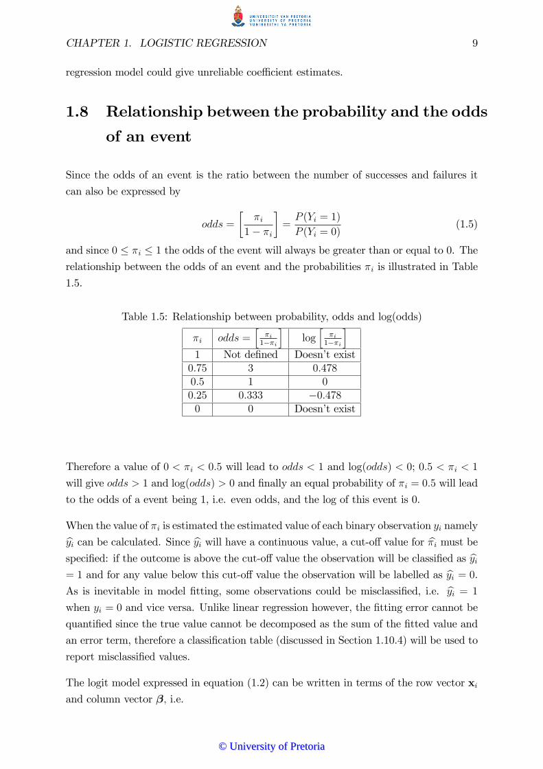
Since the odds of an event is the ratio between the number of successes and failures it
can also be expressed by
odds =
��i
1� �i
�=P (Yi = 1)
P (Yi = 0)(1.5)
and since 0 � �i � 1 the odds of the event will always be greater than or equal to 0. Therelationship between the odds of an event and the probabilities �i is illustrated in Table
1.5.
Table 1.5: Relationship between probability, odds and log(odds)
�i odds =h
�i1��i
ilogh
�i1��i
i1 Not de�ned Doesn�t exist0:75 3 0:4780:5 1 00:25 0:333 �0:4780 0 Doesn�t exist
Therefore a value of 0 < �i < 0:5 will lead to odds < 1 and log(odds) < 0; 0:5 < �i < 1
will give odds > 1 and log(odds) > 0 and �nally an equal probability of �i = 0:5 will lead
to the odds of a event being 1, i.e. even odds, and the log of this event is 0.
When the value of �i is estimated the estimated value of each binary observation yi namelybyi can be calculated. Since byi will have a continuous value, a cut-o¤ value for b�i must bespeci�ed: if the outcome is above the cut-o¤ value the observation will be classi�ed as byi= 1 and for any value below this cut-o¤ value the observation will be labelled as byi = 0.As is inevitable in model �tting, some observations could be misclassi�ed, i.e. byi = 1
when yi = 0 and vice versa. Unlike linear regression however, the �tting error cannot be
quanti�ed since the true value cannot be decomposed as the sum of the �tted value and
an error term, therefore a classi�cation table (discussed in Section 1.10.4) will be used to
report misclassi�ed values.
The logit model expressed in equation (1.2) can be written in terms of the row vector xiand column vector �; i.e.
©© UUnniivveerrssiittyy ooff PPrreettoorriiaa

CHAPTER 1. LOGISTIC REGRESSION 10
log
��i
1� �i
�= xi�: (1.6)
Taking the antilog of equation (1.6) yields
elogh
�i1��i
i= exi�
i.e.�i
1� �i= exi�
i.e. �i = exi�(1� �i)i.e. �i + �ie
xi� = exi�
) �i =exi�
1 + exi�(1.7)
and
1� �i = 1� exi�
1 + exi�
=1 + exi� � exi�1 + exi�
=1
1 + exi�: (1.8)
Therefore �i = P (Yi = 1) = exi�
1+exi�(Cox and Snell 1989, p. 19) or equivalently, if the
equation is multiplied with�e�xi�
e�xi�
�the probability of a success is given by
�i = P (Yi = 1) =1
1 + e�xi�: (1.9)
To visualise how the function in equation (1.7) responds to di¤erent values of �i one can
simplify the model in equation (1.7) to include only one explanatory variable, say the jth
covariate, and no constant term expressed by
�i =exij�j
1 + exij�j: (1.10)
Figures 1.1 and 1.2 (Allison 2012, p. 91), illustrate the logistic curve of the probability
�i at di¤erent values of xij when �j is positive and when �j is negative. It can be noted
from Figure 1.1 that there is an upward trend when �j > 0; and from Figure 1.2 that
there is a downward trend when �j < 0:
©© UUnniivveerrssiittyy ooff PPrreettoorriiaa

CHAPTER 1. LOGISTIC REGRESSION 11
Figure 1.1: Logistic curve for values where �j > 0
x
Prob
abilit
y
1.0
0.8
0.6
0.4
0.2
0.0
Figure 1.2: Logistic curve for values where �j < 0
x
Prob
abilit
y
1.0
0.8
0.6
0.4
0.2
0.0
1.9 Estimating the parameters
To use the function in equation (1.2) one needs to determine the elements of the column
vector �: One of the most popular methods to estimate unknown coe¢ cients is using
maximum likelihood (ML) estimation. Since the values of y = [y1; :::; yn]T are assumed to
be independent, the likelihood function (Collett 2003, p. 67) of the n binary observations
as a function of � is:
l(�) = P (Y1 = y1; Y2 = y2; :::; Yn = yn; �1; :::; �n) =nQi=1
�yii (1� �i)1�yi : (1.11)
The log-likelihood function of � = [�0; :::; �m]T is obtained by determining the natural
logarithm of the likelihood function in equation (1.11) and by rewriting equation (1.6) as
log(�i) = xi� + log(1� �i), that is
©© UUnniivveerrssiittyy ooff PPrreettoorriiaa

CHAPTER 1. LOGISTIC REGRESSION 12
log l(�) =nPi=1
fyi log �i + (1� yi) log(1� �i)g
=nPi=1
fyi(xi� + log(1� �i)) + (1� yi) log(1� �i)g
=nPi=1
fyixi� + yi log(1� �i) + log(1� �i)� yi log(1� �i)g
=nPi=1
fyixi� + log(1� �i)g
=nPi=1
�yixi� � log(1 + e(xi�))
: (1.12)
The ML estimate for �j; j = 0; 1; :::;m can be obtained by getting the derivative of
equation (1.12) with respect to �j and setting this derivative equal to 0. The derivative
of equation (1.12) for j = 1; 2; :::;m as given in Heinze and Schemper (2002) is
U(�j) =@ log l(�)
@�j
=nXi=1
yixij �nXi=1
exij�j(xij)
1 + exij�j
=nXi=1
yixij �nXi=1
�ixij
=nXi=1
(yi � �i)xijset= 0. (1.13)
The derivative of equation (1.12) with respect to �0; set equal to 0; simpli�es to
U(�0) =@ log l(�)
@�0
=nXi=1
yi �nXi=1
e�0
1 + e�0
=nXi=1
yi �nXi=1
�iset= 0 (1.14)
since xi0 = 1 for 8i: From equation (1.14) and Hosmer and Lemeshow (2001, p. 10) it
can be noted that the solution for the sum of the observed values can be expressed as
nXi=1
yi =nXi=1
b�i (1.15)
where b�i is the predicted values of �i:
©© UUnniivveerrssiittyy ooff PPrreettoorriiaa

CHAPTER 1. LOGISTIC REGRESSION 13
In logistic regression the equations given in (1.13) and (1.14) are nonlinear in �j;j =
0; 1; :::;m and thus require special methods to solve. The solution of � from equations
(1.13) and (1.14) which is called the ML estimator (b�); is obtained by using iterativemethods. For a simple logistic regression model, a model is saturated when the number
of groups for the independent variable, k, equals the number of unknown parameters
(m + 1) in the model. For saturated models the equations in (1.13) and (1.14) can be
solved explicitly for the ML estimator b�: Examples hereof include the case where thebinary response variable can be found as a function with only one variable X (with
two possible outcomes) such that observed values obtained can be expressed in a 2 � 2contingency table as expressed in Table 1.2. In this case the observed frequencies can
be used in the natural logarithm of the cross product ratio to obtain the ML estimates
(Allison et al., 2004)
b� = log f11f22f12f21
(1.16)
where fij indicates the frequency for the ith row and jth column in the 2� 2 contingencytable.
For most models, however, the model cannot be classi�ed as saturated and therefore no
explicit solution can be determined. In this scenario the ML estimates have to be obtained
with numerical methods, the most often applied method being Newton-Rhapson.
Consider the ith row vector xi = (1; xi1; xi2; :::xim) as an (m+1)� 1 column vector of thecovariates for observation i i.e. xTi : The �rst derivative of the log-likelihood with respect
to �; set equal to 0; can be found (Allison 2012, p. 44) as
U(�)=@ log l(�)
@�=
nXi=1
xTi yi �nXi=1
xTi (1 + e�xTi )�1 (1.17)
whereU(�) is a (m+1)�1 column vector of partial derivativesh@ log l(�)@�0
; @ log l(�)@�1
; :::; @ log l(�)@�m
iTand is also known as the gradient or score function. The second derivative with respect
to � of the log-likelihood function set equal to 0 is indicated (Allison 2012, p. 44) by
I(�)=@2 log l(�)
@�@�0 = �
nPi=1
xTi xi(1 + e�xTi )�1(1� (1 + e�xTi )�1) (1.18)
where I(�) is a matrix of second partial derivatives and is also known as the Hessian
matrix. The Hessian matrix is not only used to estimate coe¢ cients from the well de-
veloped theory of ML estimation (Rao, 1973), but is also used to estimate the variances
and covariances of the estimated coe¢ cients.
©© UUnniivveerrssiittyy ooff PPrreettoorriiaa

CHAPTER 1. LOGISTIC REGRESSION 14
The diagonal and o¤-diagonal elements of the Hessian matrix can be expressed (Hosmer
& Lemeshow 2001, p. 34) by
@2 log l(�)
@�2j= �
nXi=1
x2ij�i(1� �i) (1.19)
and
@2 log l(�)
@�j@�l= �
nXi=1
xijxil�i(1� �i) (1.20)
for j; l = 0; 1; 2; :::;m. The variances and covariances of the estimated coe¢ cients are
obtained from the inverse of the Hessian matrix i.e.
V ar(�) = I�1(�): (1.21)
The value for V ar(�) at the estimated value b� will be donated by V ar(b�), where thevalues in this matrix for the jth coe¢ cient estimate will be expressed by dV ar( b�j) anddCov( b�j; b�l):The estimates for � is then calculated (Allison 2012, p. 44) by the Newton-Rhapson
algorithm formulated by
�new = �old � I�1(�old)U(�old) (1.22)
where I�1(�) is the inverse of the Hessian matrix I(�): The column vector of starting
values (�old) is substituted on the right hand side of equation (1.22), this will yield the
new value (�new) on the left hand side of (1.22), �new is then used on the right hand side
of the equation to obtain the next new value on the left hand side. This process will be
repeated until the left hand side of the equation is equal to the right hand side which is an
indication that the process converged. This process usually takes fewer than 25 iterations
for convergence, if the process did not converge after 25 iterations the chance that it will
converge is very low. When the process does not converge, it is a strong indication that
separation is present in the data, which will be discussed in Chapter 2.
1.10 Goodness of �t
Many goodness-of-�t measures exist to show how well a given logistic regression model
�ts the data. There is however no overall best method which can be singled out to assess
the adequacy or inadequacy of a given logistic regression model. Each method has its
own advantages and disadvantages depending on the sample size, type of covariates used,
etc. Four di¤erent types of methods will be considered, the �rst method comprises of
©© UUnniivveerrssiittyy ooff PPrreettoorriiaa

CHAPTER 1. LOGISTIC REGRESSION 15
tests which are based on covariate patterns and consist of the Pearson�s chi-square test
(Pearson, 1900) and the deviance test. The second method uses estimated probabilities
from the assumed model which is known as Hosmer and Lemeshow�s bC and bH tests. The
third method is informal model �t statistics, followed by using a tabular method, the
classi�cation tables. There are a number goodness-of-�t models available in practice and
the interested reader is referred to Liu (2007) and Hosmer and Lemeshow (2001).
1.10.1 Pearson�s chi-square test and deviance test
In linear regression the signi�cance of a model is found by computing the squared distance
between the observed and the predicted outcome value also known as the SSE. This value
indicates how close the model correctly predicted the outcome variable. If the size of the
SSE is large it implies a large distance between the observed and the estimated outcome
which is an indication that the model is not a good predictor. In logistic regression
the same approach is followed i.e. to take the di¤erence between the observed and the
predicted outcome. According to Hosmer and Lemeshow (2001) the deviance statistic for
logistic regression plays the same role as the SSE plays in linear regression.
To derive the Pearson chi-square statistic, assume n independent observations from a
Bernoulli distribution where the probability of a success for a single observation is given
by �i. Then the logistic regression model can be derived as described in Section 1.5. The
estimated parameters of the logistic regression model can be obtained with numerical
methods as discussed in Section 1.9. Suppose a logistic regression model is derived as in
equation (1.2), then if the �tted model hasm covariates, each observation yi; i = 1; 2; :::; n
has a single covariate set xi = [xi0; xi1; :::; xim] which is represented in a single row of X
in (1.3). As discussed in Section 1.7 two types of covariate patterns can exist in a data
set. The �rst is where each observation has its own unique covariate set and there are no
tied covariate sets (i.e. q = n), this is also referred to as a sparse data set. The second
type is where more than one observation share the same covariate set (i.e. q < n).
By considering the second type of covariate pattern (q < n), if vc number of observations
in the cth covariate class share the same covariate set thenqXc=1
vc = n: If ns is the total
number of successes and nf is the total number of failures over all the covariate classes
then n = ns + nf : If the total number of successes in the cth covariate class is given by
yc1 and the total number of failures is given by yc0 thenqXc=1
yc1 = ns andqXc=1
yc0 = nf :
The expected number of successes for the cth covariate class can be given by (Hosmer
and Lemeshow 2001, p. 145)
©© UUnniivveerrssiittyy ooff PPrreettoorriiaa

CHAPTER 1. LOGISTIC REGRESSION 16
cyc1 = vc b�c (1.23)
where b�c is the ML estimator of �c of the cth covariate class given by b�c = excb�
1+excb� .The likelihood function in equation (1.11) is that of n independent observations from
a Bernoulli distribution. Now we have the case where vc observations share the same
covariate set and therefore a likelihood function can be derived in terms of vc, yc1, �cgiven by (Liu 2007, p. 20)
l(�) =qQc=1
vc
yc1
!�yc1c (1� �c)vc�yc1 (1.24)
and the natural logarithm of the function in equation (1.24) is given by
log l(�) =
qXc=1
(log
vc
yc1
!+ yc1 log(�c) + (vc � yc1) log(1� �c)
): (1.25)
For a speci�c covariate pattern of covariate class c the Pearson residual (Hosmer and
Lemeshow 2001, p. 145) is given by
r(yc1; b�c) = (yc1 � vc b�c)pvc b�c(1� b�c) (1.26)
and the Pearson chi-square test statistic is expressed by
�2 =
qXc=1
r(yc1; b�c)2 (1.27)
with q � (m+ 1) degrees of freedom.
The deviance residual for the cth covariate class is given by (Hosmer and Lemeshow 2001,
p. 146)
d(yc1; b�c) = ��2 �yc1 log� yc1vc b�c
�+ (vc � yc1) log
�(vc � yc1)vc(1� b�c)
���1=2: (1.28)
If the cth covariate class has no successes (yc1 = 0) it results in�yc1vcc�c�= 0 then the
deviance residual can be calculated by
d(yc1; b�c) = �p2vc jlog(1� b�c)j: (1.29)
Similarly, if only successes are observed in the cth covariate class (yc1 = vc) it leads to�(vc�yc1)vc(1�c�c)
�= 0 and the deviance residual can be calculated by
d(yc1; b�c) =p2vc jlog( b�c)j: (1.30)
©© UUnniivveerrssiittyy ooff PPrreettoorriiaa

CHAPTER 1. LOGISTIC REGRESSION 17
From equations (1.28), (1.29) and (1.30) the deviance statistic can be calculated by
D =
qXc=1
d(yc1; b�c)2: (1.31)
If the model is correct, the deviance test statistic is approximately a chi-square distribu-
tion with q � (m+ 1) degrees of freedom.
When the �rst covariate type (q = n) is present in a data set, i.e. vc = 1 for 8c, Pearson�sstatistic reduces to (by using equation (1.15)) as shown in McCullagh and Nelder (1989,
p. 121)
�2 =
qXc=1
(yc1 � b�c)2b�c(1� b�c)=
nXi=1
(yi � b�i)2b�i(1� b�i)=
nXi=1
(yi � 2yi b�i + b�i2)b�i(1� b�i)=
nXi=1
(yi � 2y2i + y2i )yi(1� yi)
=nXi=1
(yi � y2i )yi(1� yi)
=nXi=1
yi(1� yi)yi(1� yi)
= n: (1.32)
From equation (1.32) one can note that the Pearson chi-square statistic is reduced to the
sample size which is not a very useful test for goodness-of-�t.
Similarly when the �rst covariate type is present in a data set, the deviance residual from
equation (1.28) is reduced to
d(yi; b�i) = ��2 �yi log� yib�i�+ (1� yi) log
�(1� yi)(1� b�i)
���1=2(1.33)
since vc = 1, yc1 = yi and all classes are of size 1. The only two possible values for yi is 0
or 1 which implies that the values for (1� yi) ln(1� yi) and yi ln yi will be reduced to 0for either case. By taking this into consideration, combined with the result from equation
(1.15), the deviance test statistic in equation (1.31) can be rewritten, as shown by (Liu
2007, p. 22) , to be
©© UUnniivveerrssiittyy ooff PPrreettoorriiaa
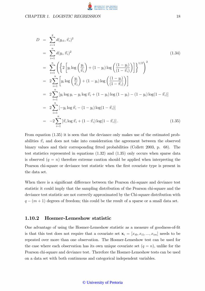
CHAPTER 1. LOGISTIC REGRESSION 18
D =
qXc=1
d(yc1; b�c)2=
nXi=1
d(yi; b�i)2 (1.34)
=
nXi=1
�2
�yi log
�yib�i�+ (1� yi) log
�(1� yi)(1� b�i)
���1=2!2
= 2nXi=1
�yi log
�yib�i�+ (1� yi) log
�(1� yi)(1� b�i)
��= 2
nXi=1
[yi log yi � yi log b�i + (1� yi) log (1� yi)� (1� yi) log(1� b�i)]= 2
nXi=1
[�yi log b�i � (1� yi) log(1� b�i)]= �2
nXi=1
[b�i log b�i + (1� b�i) log(1� b�i)] : (1.35)
From equation (1.35) it is seen that the deviance only makes use of the estimated prob-
abilities b�i and does not take into consideration the agreement between the observedbinary values and their corresponding �tted probabilities (Collett 2003, p. 68). The
test statistics represented in equations (1.32) and (1.35) only occurs when sparse data
is observed (q = n) therefore extreme caution should be applied when interpreting the
Pearson chi-square or deviance test statistic when the �rst covariate type is present in
the data set.
When there is a signi�cant di¤erence between the Pearson chi-square and deviance test
statistic it could imply that the sampling distribution of the Pearson chi-square and the
deviance test statistic are not correctly approximated by the Chi-square distribution with
q � (m+ 1) degrees of freedom; this could be the result of a sparse or a small data set.
1.10.2 Hosmer-Lemeshow statistic
One advantage of using the Hosmer-Lemeshow statistic as a measure of goodness-of-�t
is that this test does not require that a covariate set xi = [xi0; xi1; :::; xim] needs to be
repeated over more than one observation. The Hosmer-Lemeshow test can be used for
the case where each observation has its own unique covariate set (q = n), unlike for the
Pearson chi-square and deviance test. Therefore the Hosmer-Lemeshow tests can be used
on a data set with both continuous and categorical independent variables.
©© UUnniivveerrssiittyy ooff PPrreettoorriiaa

CHAPTER 1. LOGISTIC REGRESSION 19
There are two di¤erent types of Hosmer-Lemeshow tests available (Liu 2007, p. 24), the
one is based on predetermined cut-o¤ values of the estimated probability of a success and
is indicated by bH. To calculate bH, ten groups are formed by setting the upper interval forthe �tted probabilities for each group to 0:1; 0:2; :::; 1. This may however lead to groups
with small and/or unequal sizes which is why this particular method is not often used in
practice and therefore will not be discussed any further.
The second statistic, bC; is more prevalent and will be discussed. This test is based on thepercentiles of the estimated probabilities. The �rst step to determine bC is to calculate
the estimated probabilities under the assumed logistic regression model derived for the
speci�c data set (as derived in equation (1.7)) of all the observations. The observations
are then sorted into ascending order according to the corresponding �tted probabilities.
From this ordered list the observations are grouped. The groups can be selected manually
such that the groups have equal sizes:
Suppose there is a total of a groups where each group is of size va. In each of these groups
the observed values for the dependent variable yi; i = 1; 2; :::; a; are added to obtain the
observed number of successes, oi in that group. Similarly, the �tted probabilities in
each group are added to obtain the estimated expected number of successes, ei: In each
group the average success probability is the expected number of successes divided by
the total number of observations in that group, i.e. b�i = eiva:Using this information the
Hosmer-Lemeshow test statistic is given by (Hosmer and Lemeshow 2001, p. 148)
bC = aXi=1
(oi � va b�i)2va b�i(1� b�i) : (1.36)
This statistic is an approximate chi-square distribution with (a � 2) degrees of freedomwhen the �tted model is appropriate. This leads to a formal goodness-of-�t hypothesis
test where each observation has its own unique covariate set. This value should be
interpreted with caution since the value is greatly in�uenced by the total number of
observations, the number of observations within each group and how the values are split
into di¤erent groups. Care should especially be taken when interpreting this value when
the number of covariate patterns are less than the number of observations (q < n), as
shown in Bertolini et al. (2000). Any conclusion based on this statistic should only be
taken as a guideline on assessing the goodness-of-�t of a logistic regression model.
1.10.3 Model �t statistics
Penalized �t statistics, as discussed in (Allison 2012, p. 22) can be used to informally
compare models with di¤erent number of covariates against each other; these values can
©© UUnniivveerrssiittyy ooff PPrreettoorriiaa

CHAPTER 1. LOGISTIC REGRESSION 20
however not be used to construct a formal hypothesis testing such as the Pearson chi-
square, deviance test statistic and Hosmer-Lemeshow statistic.
The most fundamental test of the model �t statistics is the maximised value of the log
likelihood function as de�ned in equation (1.11) multiplied by �2. The value of
�2LogL (1.37)
is greatly dependent on the number of observations and the number of covariates consid-
ered in the data set. A high value for �2LogL is usually a indication of a badly �ttedmodel, but since this value is a¤ected by the data set that is used, it is advised to only
use this value as a comparative measure for di¤erent models �tted on the same data set.
If a data set has more covariates, the value of �2LogL tends to decrease, if the numberof observations in the data set increases the value of �2LogL tends to be in�ated.
Since the �2LogL value decreases (showing a better �t) as the number of covariatesincreases, another measure needs to be considered which penalises models with more
covariates. The Akaike�s information criterion (AIC) places such a penalty on models
since it is calculated by
AIC = �2LogL+ 2k (1.38)
where k is the number of covariates plus the intercept term, therefore k = m + 1. For
each additional covariate introduced in a model the value of �2LogL is thus penalised(increased) by a factor of 2.
Schwarz criterion (SC) is a statistic that even more severely penalises �2LogL for eachadditional covariate added and is given by
SC = �2LogL+ k log n (1.39)
Each additional covariate in the model is now penalised by a factor of k log n where k =
m+1 and log n is the natural logarithm of the number of observations used in the model.
For example if a model is built based on a sample of 50 observations, each additional
covariate introduced in the model will be penalised by a factor of log(50) = 3:912.
1.10.4 Classi�cation tables
The methods and tests mentioned up to this stage involve formal hypothesis testing
and informal model �t statistics to assess whether the logistic regression model �ts the
data adequately. These methods however do not allow a visual representation of the
©© UUnniivveerrssiittyy ooff PPrreettoorriiaa
CHAPTER 1. LOGISTIC REGRESSION 21
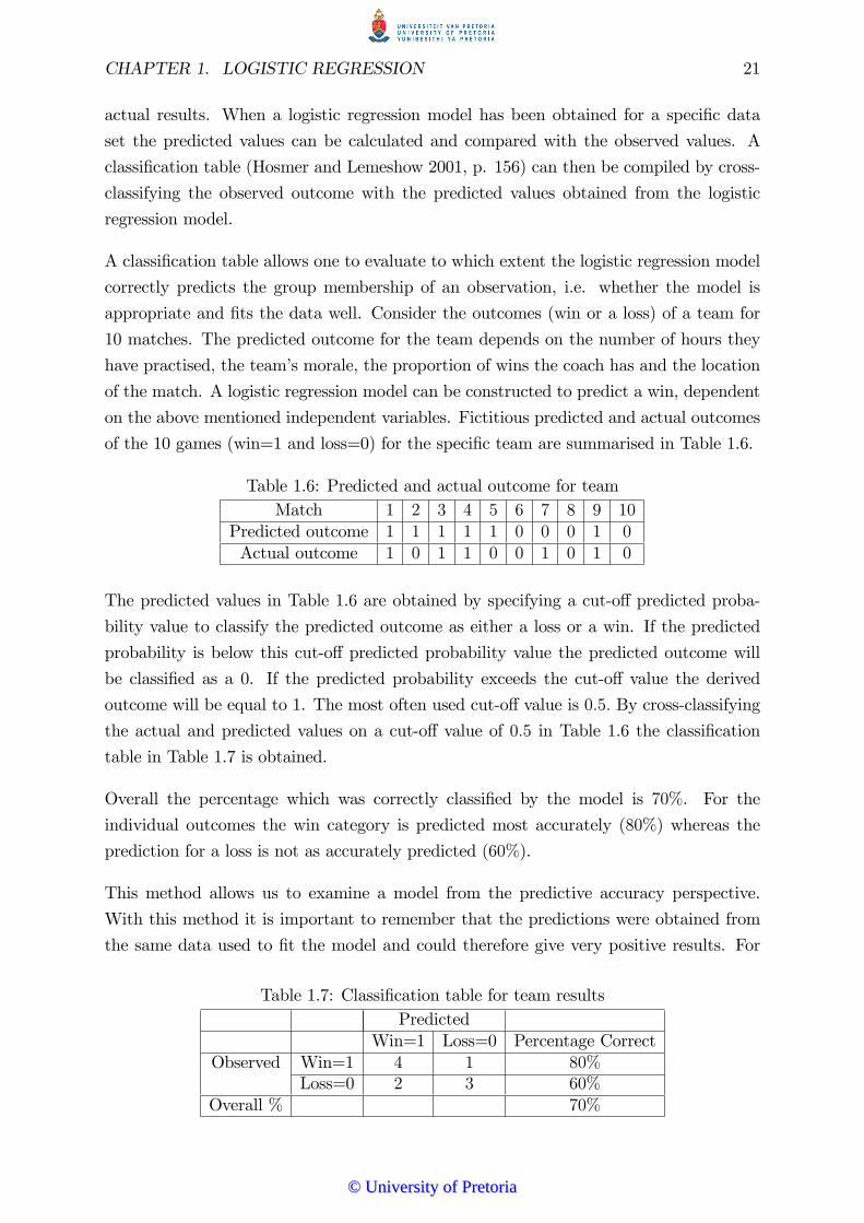
actual results. When a logistic regression model has been obtained for a speci�c data
set the predicted values can be calculated and compared with the observed values. A
classi�cation table (Hosmer and Lemeshow 2001, p. 156) can then be compiled by cross-
classifying the observed outcome with the predicted values obtained from the logistic
regression model.
A classi�cation table allows one to evaluate to which extent the logistic regression model
correctly predicts the group membership of an observation, i.e. whether the model is
appropriate and �ts the data well. Consider the outcomes (win or a loss) of a team for
10 matches. The predicted outcome for the team depends on the number of hours they
have practised, the team�s morale, the proportion of wins the coach has and the location
of the match. A logistic regression model can be constructed to predict a win, dependent
on the above mentioned independent variables. Fictitious predicted and actual outcomes
of the 10 games (win=1 and loss=0) for the speci�c team are summarised in Table 1.6.
Table 1.6: Predicted and actual outcome for teamMatch 1 2 3 4 5 6 7 8 9 10
Predicted outcome 1 1 1 1 1 0 0 0 1 0Actual outcome 1 0 1 1 0 0 1 0 1 0
The predicted values in Table 1.6 are obtained by specifying a cut-o¤ predicted proba-
bility value to classify the predicted outcome as either a loss or a win. If the predicted
probability is below this cut-o¤ predicted probability value the predicted outcome will
be classi�ed as a 0. If the predicted probability exceeds the cut-o¤ value the derived
outcome will be equal to 1. The most often used cut-o¤ value is 0:5: By cross-classifying
the actual and predicted values on a cut-o¤ value of 0:5 in Table 1.6 the classi�cation
table in Table 1.7 is obtained.
Overall the percentage which was correctly classi�ed by the model is 70%. For the
individual outcomes the win category is predicted most accurately (80%) whereas the
prediction for a loss is not as accurately predicted (60%).
This method allows us to examine a model from the predictive accuracy perspective.
With this method it is important to remember that the predictions were obtained from
the same data used to �t the model and could therefore give very positive results. For
Table 1.7: Classi�cation table for team resultsPredicted
Win=1 Loss=0 Percentage CorrectObserved Win=1 4 1 80%
Loss=0 2 3 60%Overall % 70%
©© UUnniivveerrssiittyy ooff PPrreettoorriiaa

CHAPTER 1. LOGISTIC REGRESSION 22
example if a correctly classi�ed percentage of wins is 70%; it suggests a good �t on the
face of it. If however it is much more likely that a team will win than lose, 70% correctly
classi�ed as a win may be a bad prediction. It should be borne in mind that classi�cation
is susceptible to the relative sizes of the two groups and always promotes classi�cation
into the group with the larger size.
Classi�cation is not just dependent on the sample size but also on the predictive outcome
that was obtained from the model. To illustrate this, consider (Hosmer and Lemeshow,
2001) a data set with 100 patients where the predictive probability to have a disease isb� = 0:51 for all 100 patients. If the cut-o¤ value is 0:5 and considering that the modelis appropriate would imply that 51 patients have the disease and 49 does not. Then 51
would fall above the cut-o¤ value and would be correctly classi�ed, whereas 49 out of
the 100 would be misclassi�ed. Therefore classi�cation tables should only be utilised as
an illustrative measure of the predictive outcome. It is good practice to keep a separate
validation sample which can be used to evaluate the predictive accuracy of the model.
1.11 Signi�cance of coe¢ cients
1.11.1 Test Statistics
When considering which of the covariates to include in a model, it is important to con-
sider the following question: does the model that include this speci�c covariate predict
the outcome better than a model that does not include this speci�c covariate? To an-
swer this question one can compare the output of a model that includes this particular
covariate with one that does not. From this (in addition to a few tests mentioned below)
one can decide which covariates to include in the model. It is important to remember in
the situation when a covariate is categorical and dummy variables were used to represent
this covariate, that these dummy variables form one group. Therefore if the categorical
covariate is excluded from the model, all the dummy variables which represent this co-
variate must be excluded. Section 1.11 just focuses on the signi�cance of the estimated
coe¢ cients where the signi�cance of a model as a whole (goodness-of-�t) is discussed in
Section 1.10.
One way to test the signi�cance of a coe¢ cient representing covariate j is to compute
the di¤erence of the deviance (as de�ned in equation (1.31)) when the covariate is not
included in the model and when the covariate is included in the model, shown by (Hosmer
and Lemeshow 2001, p. 14)
G = D(model without the covariate)�D(model with the covariate). (1.40)
©© UUnniivveerrssiittyy ooff PPrreettoorriiaa

CHAPTER 1. LOGISTIC REGRESSION 23
From equation (1.40) the likelihood ratio statistic can be explained. For any speci�c data
set, the derived ML estimates can be used to set up the current model. The maximised
likelihood under this current model can be denoted by cLc: The current model can how-ever not be used on its own since it is dependent on the number of observations and
covariates used and therefore needs to be compared to a baseline model. The baseline
model typically used is one that perfectly �ts the data by building a model for which the
�tted values match the actual values. This baseline model is a saturated model. The
maximised likelihood of this saturated model is denoted by cLs: From this the likelihood
ratio (LR) is given by (Collett 2003, p. 66)
LR = �2 logcLccLs : (1.41)
Under the null hypothesis that �j is equal to 0, LR follows a chi-square distribution with
degrees of freedom equal to the di¤erence in the number of parameters estimated by the
two models. For this test a large sample size n is required.
Before excluding any of the coe¢ cients, the univariate Wald statistic also needs to be
considered, it is given by (Hosmer and Lemeshow 2001, p. 37)
WALDj =b�jcSE( b�j) (1.42)
where the standard error of the estimated coe¢ cients �j; j = 0; 1; :::;m is given by
cSE( b�j) = hdV ar( b�j)i1=2 : (1.43)
From equation (1.21), the estimated variance of the vector b� is given bydV ar(b�) = bI�1(b�): (1.44)
A formulation of the Hessian matrix (expressed by equations (1.18), (1.19) and (1.20))
can be given by bI(b�) = XTW(b�)X where X is the design matrix andW(b�) is a n � nmatrix where the diagonal elements are given by b�i(1� b�i) i.e.
W(b�) =266664b�1(1� b�1) 0 � � � 0
0 b�2(1� b�2) � � � 0... 0
. . ....
0 � � � 0 c�n(1�c�n)
377775 : (1.45)
Similarly, the matrixW(�) is a n� n matrix where the diagonal elements are given by�i(1� �i) i.e.
©© UUnniivveerrssiittyy ooff PPrreettoorriiaa
CHAPTER 1. LOGISTIC REGRESSION 24
W(�) =
266664�1(1� �1) 0 � � � 0
0 �2(1� �2) � � � 0... 0
. . ....
0 � � � 0 �n(1� �n)
377775 : (1.46)
Under the null hypothesis that a speci�c coe¢ cient is not signi�cant, the Wald statistic
will follow a standard normal distribution.
For a logistic regression model with more than one covariate the Wald statistic can be
calculated by (Hosmer and Lemeshow 2001, p. 39)
WALD = b�T hdV ar(b�)i�1 b�= b�T (XTW(b�)X)b�: (1.47)
The Wald statistic given by equation (1.47) follows a chi-square distribution with m+ 1
degrees of freedom under the null hypothesis that each of the m+ 1 coe¢ cients is equal
to 0.
The LR statistic and the Wald statistic can provide guidance as to which covariates
signi�cantly contribute to predicting the outcome. The score test can also be used to
analyse the signi�cance of the estimated parameters in the model and the interested
reader is referred to Hosmer and Lemeshow (2001, p.152). One should however not
entirely base the decisions on these tests, an overall assessment of the entire model and
the e¤ect of each of the covariates should also be considered.
1.11.2 Con�dence interval
For any estimate in statistics an interval in which this estimate falls can be calculated. For
logistic regression the endpoints for a 100(1� �)% con�dence interval for the coe¢ cient
estimate of the jth covariate is given by (Hosmer and Lemeshow 2001, p. 18)
b�j � z1��2
cSE( b�j)where z1��
2is the upper 100(1��=2)% point from the standard normal distribution andcSE( b�j) is as de�ned in equation (1.43).
©© UUnniivveerrssiittyy ooff PPrreettoorriiaa

CHAPTER 1. LOGISTIC REGRESSION 25
1.12 Conclusion
Logistic regression predicts the outcome of a dichotomous variable based on a set of co-
variates. When deriving a logistic regression model it is very important to investigate the
type of covariates in your data set. If the covariates are categorical then dummy variables
should be introduced into the model, in which case the number of covariate classes present
in the data set is more likely to be less than the sample size (q < n). For this situation
the Pearson chi-square and the deviance test can be used to test the goodness-of-�t of
the model. When the covariates used are continuous no dummy variables are required in
the logistic regression model and the data set is more likely to be sparse. In this case the
Pearson chi-square and deviance test should be applied with caution and it is advisable
to rather use the Hosmer-Lemeshow test to evaluate the model�s goodness-of-�t.
©© UUnniivveerrssiittyy ooff PPrreettoorriiaa
Chapter 2
Complete and quasi-completeseparation and overlap
2.1 Introduction
When one of the independent variables, X, can perfectly classify the observations into
the respective groups of the response variable, the likelihood function has no maximum
and therefore no �nite value can be found for the estimates of �. If the maximum
of the likelihood function does not exist, it follows that the ML estimates also do not
exist. This problem is known as monotone likelihood. Three di¤erent mutually exclusive
and exhaustive classes into which the data from a logistic regression can be classi�ed
exists (Albert and Anderson, 1984): complete separation, quasi-complete separation and
overlap. Complete and quasi-complete separation imply that only an in�nite or a zero
ML estimate could be obtained for the odds ratio which rarely can be assumed to be
true in practice. Although perfect prediction is aimed for in practice, if the sample size
is small and perfect prediction occurs, it is probably as a result of random variation and
not that of a true in�nite or zero odds ratio.
To illustrate complete separation, quasi-complete separation and overlapping data, prac-
tical examples are considered as illustrated in Allison et al. (2004). For the examples
considered in Section 2:1; 2:2 and 2:3 let xi � 0 be indicated by xi = 0 and xi > 0
be indicated by xi = 1: In Chapter 2 one independent variable will be used to predict
the outcome of the dependent variable, the coe¢ cient representing this one independent
variable is indicated by �:
26
©© UUnniivveerrssiittyy ooff PPrreettoorriiaa

CHAPTER 2. COMPLETEANDQUASI-COMPLETE SEPARATIONANDOVERLAP27
2.2 Complete separation
From Albert and Anderson (1984), complete separation occurs when there exists a (m+1)
vector of coe¢ cients � such that when xi� < 0 the outcome is yi = 0 and when xi� > 0
the outcome is yi = 1: Whenever a linear function of the independent variable Xi can
perfectly predict the response variable, complete separation occurs.
Table 2.1 contains observations from a completely separated model where there is only one
explanatory variable X and the response variable Y takes on the value yi = 0 whenever
xi < 0 and yi = 1 whenever xi � 0 for i = 1; 2; :::; 10.
Table 2.1: Example of complete separation
i 1 2 3 4 5 6 7 8 9 10xi �5 �4 �3 �2 �1 1 2 3 2 5yi 0 0 0 0 0 1 1 1 1 1
The observations in Table 2.1 can be summarised by a 2� 2 contingency table.
Table 2.2: Two-way table for complete separation
y0 1
x 0 5 01 0 5
Whenever the two o¤-diagonal cells in a 2� 2 contingency table has frequencies of 0, itis an indication of complete separation. To illustrate complete separation in X and Y
consider the scatterplot of the observed values in Table 2.1 given in Figure 2.1. From
Figure 2.1 it is noted that there is a horizontal jump from yi = 0 to yi = 1.
Figure 2.1: Scatter plot of x and y under complete separation
x
y
5.02.50.02.55.0
1.0
0.8
0.6
0.4
0.2
0.0
y01
©© UUnniivveerrssiittyy ooff PPrreettoorriiaa

CHAPTER 2. COMPLETEANDQUASI-COMPLETE SEPARATIONANDOVERLAP28
By substituting the values of the contingency table into equation (1.16) the ML estimator
is b� = log (5)(5)(0)(0)
, which does not exist. As the value of the estimator � increases, the log
likelihood does not reach a maximum value. Even though the log likelihood is bounded
by the value of 0, no signi�cant values for � can be estimated, this scenario is illustrated
by Figure 2.2 (Allison et al., 2004). Since the likelihood function is �at the diagonal
elements in the variance matrix of the coe¢ cient in equation (1.44) will be in�nite in
size, which leads to an in�nite standard error of the coe¢ cient representing the covariate.
Figure 2.2: The log-likelihood function as a function of � for complete separation
ß
Log
Like
lihoo
d
543210
0
1
2
3
4
5
6
0
2.3 Quasi-complete separation
One also gets the situation, as explained by Albert and Anderson (1984), where there
exists some (m + 1) vector of coe¢ cients � such that yi = 0 when xi� � 0 and yi = 1when xi� � 0 and for at least one category of the outcome variable the equality holds.This is known as quasi-complete separation.
An example of quasi-complete separation (Allison et al., 2004) is represented in Table
2.3, where there is once again only one explanatory variable X and the response variable
Y assumes the value of yi = 0 whenever xi < 0 and yi = 1 whenever xi > 0. There is
however one value for X, xi = 0, for which both yi = 0 and yi = 1 is observed.
Table 2.3: Example of quasi-complete separation
i 1 2 3 4 5 6 7 8 9 10 11 12xi �5 �4 �3 �2 �1 0 0 1 2 3 2 5yi 0 0 0 0 0 0 1 1 1 1 1 1
©© UUnniivveerrssiittyy ooff PPrreettoorriiaa

CHAPTER 2. COMPLETEANDQUASI-COMPLETE SEPARATIONANDOVERLAP29
Table 2.4: Two-way table for quasi-complete separation
y0 1
x 0 6 11 0 5
By summarising the values in Table 2.3 in a 2�2 contingency table, Table 2.4 is obtained.If either one of the o¤-diagonal cells in a 2� 2 contingency table contains a value of 0 itis an indication of quasi-complete separation. The observations considered in Table 2.3
can be illustrated by a scatter plot shown in Figure 2.3. For the case of quasi-complete
separation there is at least one overlapping observation when xi = 0 as seen in Figure
2.3.
Figure 2.3: Scatter plot of x and y under quasi-complete separation
x
y
5.02.50.02.55.0
1.0
0.8
0.6
0.4
0.2
0.0
y01
By substituting the values of the contingency table into equation (1.16) the ML estimator
is found by b� = log (6)(5)(0)(1)
; which does not exist. As the value of the estimator � increases,
the log likelihood does not reach a maximum value. Even though the log likelihood is
bound by some value smaller than 0, in this case bounded by �1 as seen in Figure 2.4 ,no �nite value for � can be estimated. For quasi-complete separation the standard error
in equation (1.43) will be in�nite in size. This situation is far more common in practice
than complete separation.
2.4 Overlap
When neither complete nor quasi-complete separation has occurred in the data it can
be assumed that an unique �nite solution for the ML estimates exist, this is known as
overlap (Silvapulle, 1981).
©© UUnniivveerrssiittyy ooff PPrreettoorriiaa
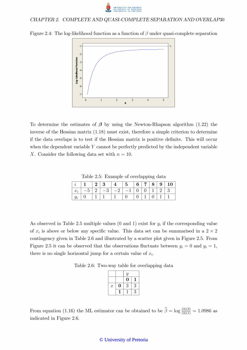
CHAPTER 2. COMPLETEANDQUASI-COMPLETE SEPARATIONANDOVERLAP30
Figure 2.4: The log-likelihood function as a function of � under quasi-complete separation
ß
Log
Like
lihoo
dFu
nctio
n
543210
1
2
3
4
5
6
7
1
To determine the estimates of � by using the Newton-Rhapson algorithm (1.22) the
inverse of the Hessian matrix (1.18) must exist, therefore a simple criterion to determine
if the data overlaps is to test if the Hessian matrix is positive de�nite. This will occur
when the dependent variable Y cannot be perfectly predicted by the independent variable
X. Consider the following data set with n = 10.
Table 2.5: Example of overlapping data
i 1 2 3 4 5 6 7 8 9 10xi �5 2 �3 �2 �1 0 0 1 2 3yi 0 1 1 1 0 0 1 0 1 1
As observed in Table 2.5 multiple values (0 and 1) exist for yi if the corresponding value
of xi is above or below any speci�c value. This data set can be summarised in a 2 � 2contingency given in Table 2.6 and illustrated by a scatter plot given in Figure 2.5. From
Figure 2.5 it can be observed that the observations �uctuate between yi = 0 and yi = 1,
there is no single horizontal jump for a certain value of xi:
Table 2.6: Two-way table for overlapping data
y0 1
x 0 3 31 1 3
From equation (1.16) the ML estimator can be obtained to be b� = log (3)(3)(3)(1)
= 1:0986 as
indicated in Figure 2.6.
©© UUnniivveerrssiittyy ooff PPrreettoorriiaa

CHAPTER 2. COMPLETEANDQUASI-COMPLETE SEPARATIONANDOVERLAP31
Figure 2.5: Scatter plot of x and y for overlapping data
x
y
4321012345
1.0
0.8
0.6
0.4
0.2
0.0
y01
Figure 2.6: The log-likelihood function as a function of � for overlapping data
ß
Log
likel
ihoo
dfu
nctio
n
2.01.51.00.50.0
6.4
6.5
6.6
6.7
6.8
6.9
1.1
2.5 Identifying complete or quasi-complete separa-
tion
The process of identifying whether a data set exhibits complete or quasi-complete separa-
tion is very important to be able to report signi�cant estimators for the logistic regression
model. Di¤erent statistical software programs have been tested with the data set repre-
sented in Tables 2.1 and 2.3 by Allison et al. (2004) to asses which of the programs give
applicable warnings of possible separation in the model. Only MINITAB, SAS GEN-
MOD, SAS LOGISTIC, SAS CATMOD and SPSS will be considered to compare with
results for 2013 since these are the software packages readily available at the University
of Pretoria. Table 2.7 indicates the warning which is given by the program, whether the
applicable program gives false convergence, reports unreliable estimates and �nally if the
program reports LR statistics.
The study done in Allison et al. (2004) is based on software that were available in 2002.
©© UUnniivveerrssiittyy ooff PPrreettoorriiaa

CHAPTER 2. COMPLETEANDQUASI-COMPLETE SEPARATIONANDOVERLAP32
Table 2.7: Computer packages under complete and quasi-complete separation
Results obtained by Allison et al. (2004)Program Warning Messages False Conv. Report Est. LR Stats
Comp. Quasi. Comp. Quasi. Comp. Quasi. Comp. Quasi.MINITAB * *
SAS GENMOD A * * * * *SAS LOGISTIC C C * *SAS CATMOD A A * * * *
SPSS C * *Results obtained for 2013
Program Warning Messages False Conv. Report Est. LR StatsComp. Quasi. Comp. Quasi. Comp. Quasi. Comp. Quasi.
MINITAB D, E; H D, E; H * *SAS GENMOD J * * * * * *SAS LOGISTIC K, F, E L, F, E * *SAS CATMOD G G * * * *
SPSS H;I H;I * *
A: Ambiguous WarningC: Clear WarningD: Algorithm did not convergeE: Results may be unreliableF: MLE does not existG: Parameter estimates are in�niteH: Max number of iterations reachedI: No solution could be foundJ: Hessian matrix not positive de�niteK: Complete SeparationL: Quasi-complete Separation
Comparing the results in Table 2.7 from 2002 to 2013, one observes that some of the
programs have improved whilst some stayed the same.
One of the computer packages that improved a great deal is MINITAB, even though it
still reports estimates: from no warning in 2002 to giving a warning that even if the
maximum number of iterations have been reached, no convergence was reached and the
results obtained could be unreliable in 2013.
The SAS GENMOD procedure still reports false converge, values for the estimates and
LR statistics. The warning message in 2002 was seen as ambiguous, the message as
seen in 2013 reports that the Hessian matrix is not positive de�nite. This warning only
occurs when quasi-complete separation is present in the data set; for complete separation
no warning is given. If an user has a good understanding of how the coe¢ cients are
estimated, he or she would know that if the Hessian is not positive de�nite it will not be
possible to obtain reliable estimates.
©© UUnniivveerrssiittyy ooff PPrreettoorriiaa

CHAPTER 2. COMPLETEANDQUASI-COMPLETE SEPARATIONANDOVERLAP33
A clear warning is still given by SAS LOGISTIC in 2013; it reports estimates but gives
a clear warning that the estimates are in�nite and that the ML estimates does not exist.
The SAS LOGISTIC procedure is the only program from the list in Table 2.7 that gives
a warning "Complete separation" or "Quasi-complete separation" if either one of those
scenarios occur within the data set.
The third SAS procedure to be considered is the SAS CATMOD procedure, this procedure
still gives false convergence and reports estimates, but from an ambiguous warning in
2002 it now reports that the parameter estimates are in�nite, which gives the user of the
program a good indication to apply caution when interpreting the estimated parameters.
The �nal program considered is SPSS. In 2002 this program gave a clear warning but
only for complete separation and it reported false convergence and estimates for quasi-
complete separation. In 2013 it still reports estimates but now gives a warning that
no solution could be found even though the maximum number of iterations have been
reached for both complete and quasi-complete separation.
2.6 Conclusion
When constructing a logistic regression model it is not always the case that the coe¢ cient
estimates will exist or, if the coe¢ cient estimates do exist, will be reliable. Therefore it
is essential to test whether complete or quasi-complete separation is present in a data set
when the dependent variable is dichotomous, especially when the sample size is small.
When complete or quasi-complete separation is present in the data set it is imperative
not to continue with the general approach to computing a logistic regression model, but
to follow a di¤erent approach. A few of these di¤erent approaches to deal with complete
or quasi-complete separation are mentioned and investigated in Chapter 3.
©© UUnniivveerrssiittyy ooff PPrreettoorriiaa

Chapter 3
Methods used to deal withseparation
3.1 Introduction
The problem of complete separation and quasi-complete separation in binomial data mod-
elling was �rst documented by Day and Kerridge (1967). As shown in Silvapulle(1981),
when the data overlaps in a logistic regression model the ML estimates exist and are
unique, if separation in the data occurs the ML estimates does not exist. A formal
criterion to distinguish between complete separation and quasi-complete separation was
proposed by Albert and Anderson (1984) as discussed in Chapter 2. It is of utmost im-
portance to know if either complete separation and quasi-complete separation is present
within the data set in order to interpret the estimated regression coe¢ cients correctly.
Numerous methods to detect complete separation or quasi-complete separation have been
developed over the years. A linear-programming method was proposed by Albert and An-
derson (1984) which indicates when the data does not overlap. This linear programming
method was extended to a mixed linear programming algorithm by Santer and Du¤y
(1986) which determines for each data set whether there is complete separation, quasi-
complete separation or if the data overlap. Christmann and Rousseeuw (2001) developed
a method not just to determine whether the data overlaps, but also to determine to which
degree the data overlap in the data set.
3.2 Di¤erent methods
3.2.1 Changing the model
34
©© UUnniivveerrssiittyy ooff PPrreettoorriiaa
CHAPTER 3. METHODS USED TO DEAL WITH SEPARATION 35
As shown in Section 2.5, to identify whether the ML estimates exist is easily managed
with most statistical software packages. The next step is to obtain a solution when
dealing with non-overlapping data. One often used method in practice is to omit some
of the covariates which is the cause of complete separation or quasi-complete separation.
This method is however not recommended, since by omitting the covariates that hold
a strong relationship to the occurrence of interest is similar to deliberately introducing
speci�cation bias, which in turn leads to biased parameter estimates.
Another approach which changes the original covariates included in the model is by
adding arti�cial data across the various patterns to "�ll the gaps" which was caused by
separation. Various techniques are available to impute observations. This method was
proposed by Clogg et al. (1991) and as with omitting covariates, changes the covariates
that hold a strong relationship with the outcome. This method is not recommended as
shown in Heinze and Schemper (2002).
If the problematic covariate is a nominal variable with more than 2 categories, for example
single, married and divorced, the categories can be grouped together. For example single
and divorced can be considered as one group and married can be seen as the other
group. This method usually solves quasi-complete separation but does not solve complete
separation. It should also be borne in mind that if the groups are merged and the observed
values are more condensed, it will not be possible to allocate the observations to the
original groups, i.e. to restore the data set back to its original dimension.
3.2.2 Working with the likelihood function
Methods based on the likelihood function are preferred to methods which change the
original data set. One option is to use exact logistic regression (Section 3.3) as proposed
by Cox and Snell (1989) but is computing-intensive. Another solution to dealing with non-
overlapping data is by penalising the likelihood function with Je¤reys prior as proposed
by Firth (1993). Firth�s method is explained in Section 3.4 and has many advantages
as shown in Heinze (2006). Firth�s method of penalising the likelihood function was
extended by Heinze and Schemper (2002) to calculate the con�dence intervals based
on this method instead of using Wald intervals which are unreliable when dealing with
non-overlapping data. If multicollinearity is present in the data set, a second penalising
term can be introduced as shown in Gao and Chen (2007). In 2003, Rousseeuw and
Christmann introduced the concept of hidden logistic regression discussed in Section 3.5.
This involves obtaining a maximum estimated likelihood estimator which always exists
and is robust to separation and outliers.
©© UUnniivveerrssiittyy ooff PPrreettoorriiaa

CHAPTER 3. METHODS USED TO DEAL WITH SEPARATION 36
Since altering the original data set is not recommended and has been shown to give
undesirable results in Heinze and Schemper (2002), this method will not be discussed
further. Exact logistic regression, Firth�s method and hidden logistic regression will be
extended on in Section 3.3 to 3.5. All three methods will be applied to practical examples
in part II where they will be compared to each other in di¤erent scenarios.
3.2.3 Other methods
Alternative methods which merit mentioning but will not be elaborated on in this dis-
sertation includes an approach using Markov chain Monte Carlo methods in which one
would work in a Bayesian paradigm. Caution is advised when using these methods since
uninformative priors can lead to no convergence of the coe¢ cient estimates and the use of
informative priors may result to misleading results as discussed in Abrahantes and Aerts
(2012) and Allison et al. (2004).
When dealing with separation one should also be aware of other properties within a data
set which could lead to misleading results. Multicollinearity can be problematic if not
dealt with correctly. Gao and Chen (2007) discuss this phenomenon and introduce a
second penalising term to address this problem. Another statistical problem which can
be observed in practice is outliers. An outlier-robust method is discussed in Rousseeuw
and Christmann (2003). These are just a few di¤erent methods to deal with certain
aspects which can be observed within a data set and one should always exercise caution
when using di¤erent methods and interpreting results.
3.3 Exact logistic regression
Exact logistic regression was �rst proposed by Cox and Snell (1989). This method is
also known as exact conditional inference. As stated by King and Ryan (2002), the
general idea of exact logistic regression is "to base inferences on exact permutational
distributions of the su¢ cient statistics that correspond to the regression parameters of
interest, conditional on �xing the su¢ cient statistic of the remaining parameters at their
observed values".
3.3.1 The ML estimates
To obtain the conditional likelihood function to estimate a speci�c parameter, consider
�rst the likelihood function given in equation (1.11) and the logit function de�ned in
©© UUnniivveerrssiittyy ooff PPrreettoorriiaa

CHAPTER 3. METHODS USED TO DEAL WITH SEPARATION 37
equation (1.2); then the unconditional likelihood function is given by (Collett 2003, p.
308)
l(�) =nQi=1
�yii (1� �i)1�yi
=nQi=1
�yii (1� �i)�yi(1� �i)1
=nQi=1
��i
1� �i
�yi(1� �i)
=nQi=1
exi�yi(1 + exi�)�1
nQi=1
exi�yi(1 + e�i)�1
=e
nPi=1
mPj=0
�jxijyi
nQi=1
(1 + e�i)(3.1)
Let tj =nPi=1
xijyi; j = 0; 1; :::;m therefore for yi = 1; tj is the sum of the values of the jth
explanatory variable and expression (3.1) can be rewritten as
l(�) =e
mPj=0
�jtj
nQi=1
(1 + e�i): (3.2)
The tj values contain all the information about the �0
js for the binary observations,
therefore the t0js are the su¢ cient statistics for the coe¢ cients. A full discussion on
su¢ cient statistics and its role in conditional inference is available in Cox and Hinkly
(1979).
Suppose we are only interested in one speci�c coe¢ cient, say �m; in which case the rest
of the parameters �0; :::; �m�1 are regarded as nuisance parameters and can be expressed
by the vector �1 = [�0; :::; �m�1]: The column vector of coe¢ cients can then be com-
posed as � = (�1; �m)T : The conditional likelihood function of �m is found by using the
unconditional likelihood function l(�) and eliminating the e¤ect of �1:
If t0; t1; :::; tm are the observed su¢ cient statistics from the random variables T0; T1; :::; Tm;
the conditional likelihood (as discussed in Collett (2003)) for �m given T0 = t0; :::; Tm = tmis given by
©© UUnniivveerrssiittyy ooff PPrreettoorriiaa

CHAPTER 3. METHODS USED TO DEAL WITH SEPARATION 38
lc(�m) = P (Tm = tmjT0 = t0; T1 = t1; :::; Tm�1 = tm�1) (3.3)
=P (T0 = t0; T1 = t1; :::; Tm = tm)
P (T0 = t0; T1 = t1; :::; Tm�1 = tm�1):
The numerator of equation (3.3), P (T0 = t0; T1 = t1; :::; Tm = tm); is simply the proba-
bility of the observed data which is the sum of the values of l(�) over all possible sets of
binary data that lead to t0; t1; :::; tm: Therefore the probability of the observed data can
be calculated by (Collett 2003, p. 309)
P (T0 = t0; T1 = t1; :::; Tm = tm) =c(t0; :::; tm)e
mPj=0
�jtj
nQi=1
(1 + e�i)(3.4)
where the number of distinct binary sequences that give the speci�ed values of t0; t1; :::; tmcan be denoted by c(t0; :::; tm): The joint distribution of
P (T0 = t0; T1 = t1; :::; Tm�1 = tm�1) can be found from equation (3.4) to be
P (T0 = t0; T1 = t1; :::; Tm�1 = tm�1) =
Pu c(t0; :::; tm�1; u)e
�mu+
m�1Pj=0
�jtj
nQi=1
(1 + e�i): (3.5)
where the summation term in the numerator is over all values for u for which
c(t0; :::; tm�1; u) � 1: Therefore the conditional likelihood function of �m from equation
(3.3), (3.4) and (3.5) can be expressed as (Collett 2003, p. 309)
lc(�m) =c(t0; :::; tm)e
mPj=0
�jtj
Pu c(t0; :::; tm�1; u)e
�mu+
m�1Pj=0
�jtj
=c(t0; :::; tm)e
�mtm+
m�1Pj=0
�jtj
Pu c(t0; :::; tm�1; u)e
�mu+
m�1Pj=0
�jtj
=c(t0; :::; tm)e
�mtmPu c(t0; :::; tm�1; u)e
�mu: (3.6)
From equation (3.6) it can be noted that the function does not depend on �1; :::; �m�1,
therefore if this function is maximised an exact parameter estimate for �m; also known
as the conditional ML estimate will be obtained.
©© UUnniivveerrssiittyy ooff PPrreettoorriiaa
CHAPTER 3. METHODS USED TO DEAL WITH SEPARATION 39
For a two-sided hypothesis test the null and alternative hypothesis is given byH0 : �m = 0
and H1 : �m 6= 0 respectively. The appropriate p-value for this hypothesis test, accordingto Collett (2003, p. 312), can be obtained by adding the probabilities of all the values of
the su¢ cient statistics of coe¢ cient �m which have a probability smaller than or equal to
that of the observed value. This is similar to a two-sided p-value for Fisher�s exact test.
This test is generally known as the conditional exact test and a discussion on this can
be found in Collett (2003). A full discussion on exact logistic regression can be found in
Cox and Snell (1989), Mehta and Patel (1995), Collett (2003) and Hosmer and Lemeshow
(2001).
For exact logistic regression the estimates of �0; :::; �m are obtainable even if empty cells
are observed in the 2 � 2 contingency table expressed in Table 1.2. Even though it ispossible to determine parameter estimates in the presence of complete or quasi-complete
separation, the drawback of this method is that it can get computationally di¢ cult as the
number of covariates and samples increase. As stated by Hosmer and Lemeshow (2001,
p. 337), when using exact logistic regression, caution should be taken when analysing
the Pearson chi-square and deviance test statistics since these tests are based on a large
sample assumption and this is not usually the case when using exact methods. It is
recommended that one should rather use visual methods like a classi�cation table to
investigate the agreement between the observed and the predicted value.
Another disadvantage of exact logistic regression method is that the su¢ cient statistics
for the di¤erent parameter estimates need to be summed over discrete patterns of co-
variate values. As stated by Zorn (2005), exact logistic regression will lead to unreliable
estimates when using a combination of both continuous and categorical covariates. There-
fore if exact logistic regression is applied to a data set which contains both categorical
and continuous covariates, caution should be applied when interpreting the coe¢ cient
estimates.
©© UUnniivveerrssiittyy ooff PPrreettoorriiaa

CHAPTER 3. METHODS USED TO DEAL WITH SEPARATION 40
3.4 Firth�s Model
Another way to approach the problem of separation is to reduce the bias that is found
in the ML estimates. The ML estimates are unbiased with asymptotic variance equal to
the inverse of the Fisher information matrix which is given by I(�) = ��1XTW(�)X:
The dispersion parameter is given by � = 1 (for a binomial distribution), X is the model
matrix andW is a n�n matrix whereW = diag(�i(1��i)) as shown in equation(1.46):For a large sample size McCullagh and Nelder(1989, p. 119) showed that
E(� � b�) = O(n�1) (3.7)
and expressed in terms of the covariate matrix
cov(b�) = (XTW(�)X)�1�1 +O(n�1)
: (3.8)
Then, by Firth (1993), the asymptotic bias of a single ML estimate b� of parameter � foran m dimensional model can be written as
b(�) =b1(�)
n+b2(�)
n2+ :::� (3.9)
The aim of Firth�s method is to reduce the bias of the parameter estimates, speci�cally by
removing the O(n�1) term. Two methods already exist where the term b1(�)nis removed
from the asymptotic bias, namely the jackknife method (Quenouille, 1949, 1956) and by
simply substituting b� for the unknown � in b1(�)n: The bias corrective parameter estimate,b�BC ; is then given by
b�BC = b� � b1(b�)n : (3.10)
Firth�s method is di¤erent from the procedures mentioned above in that the parameter
is not corrected after it is estimated, but a corrective procedure is applied to the ML
estimate (score function) before the parameter estimate is calculated.
3.4.1 The model
To illustrate this method consider the modelling of binomial observations where each
observation yi have a true probability of success equal to �i i.e.yini. The binomial
likelihood function can be expressed by (Collett 2003, p. 66)
©© UUnniivveerrssiittyy ooff PPrreettoorriiaa

CHAPTER 3. METHODS USED TO DEAL WITH SEPARATION 41
p(yij�i) =
ni
yi
!�yii (1� �i)ni�yi
=
ni
yi
!�yii (1� �i)�yi(1� �i)ni
=
ni
yi
!��i
1� �i
�yi(1� �i)ni : (3.11)
Taking the exponential of the log of this expression becomes
exp
(log
ni
yi
!��i
1� �i
�yi(1� �i)ni
!)
= exp
"log
ni
yi
!+ yi log
��i
1� �i
�+ ni log(1� �i)
#
= exp
24yi log�
�i1��i
�� [�ni log(1� �i)]1
+ log
ni
yi
!35 : (3.12)
The form of equation (3.12) is the same as that of n independent observations y1; :::; ynwith an exponential density expressed by (McCullagh and Nelder 1989, p. 28)
p(yij�i; �) = exp�(yi�i � d(�i))
ai(�)+ c(yi; �)
�; i = 1; 2; :::; n: (3.13)
Comparing equation (3.13) to equation (3.12) the functions in equation (3.12) can be iden-
ti�ed as �i = log�
�i1��i
�(i.e. �i = xi� from equation(1.2) );
d(�i) = �ni log(1 � �i), ai(�) = 1, c(yi; �) = log ni
yi
!where log
��i1��i
�= logit(�i) is
the canonical link function for the binomial distribution and �j is the canonical parame-
ter. The logit function is the canonical link function (McCullagh and Nelder 1989, p. 32)
since it is also a function of �i = E(Yi) = ni�i which can be seen by
logit(�i) = log�
�i1� �i
�= log
�ni�i
ni(1� �i)
�= log
��i
ni � �i
�= �i (�i) : (3.14)
Since �(�i) = log�
�i1��i
�=
mPj=0
xij�j then �(�i) = �i as shown in equation (1.2) and
tj =nXi=1
xijyi is the su¢ cient statistic for �j where j = 0; 1; :::;m:
©© UUnniivveerrssiittyy ooff PPrreettoorriiaa

CHAPTER 3. METHODS USED TO DEAL WITH SEPARATION 42
For a single parameter �j the ML estimate is derived as a solution of the derivative of
the log likelihood l(�) or score function set equal to 0, i.e.
@ log l(�)
@�j= U(�j) = 0: (3.15)
From equation (1.12) and the de�nition of su¢ cient statistic tj; the log likelihood function
for a single coe¢ cient �j can be expressed by
log l(�j) =nPi=1
nyixij�j � log(1 + e(xij�j))
o= tj�j � K(�j) where
K(�j) =nXi=1
log(1 + e(xij�j)). The score function (as obtained in equation(1.13)) can
then be expressed by
U(�j) =@ log l(�)
@�j=
nXi=1
(xijyi � xij�i) = tj �K 0(�j) (3.16)
which implies that the su¢ cient statistic tj only a¤ects the location of U(�j) and not the
gradient.
It can be shown (Firth, 1993) that the bias of the estimate b�j comes from the unbiasednessof the score function, E
�U(�j)
�= 0 at the correct value of �j and due to the bend in
the score function shown in Figure 3.1, U 00(�j) = K000(�j) 6= 0:
Figure 3.1: Modi�ed score function
If the score function U(�j) was a linear function of �j then Eh b�ji = �j; but since this
is clearly not the case as shown in Figure 3.1 a bias is induced in b�j : The idea behindFirth�s model is to implement a small bias in the score function to reduce the bias in b�j.A suitable modi�cation to U(�j) is given by
U�(�j) = U(�j)� i(�j)b(�j): (3.17)
©© UUnniivveerrssiittyy ooff PPrreettoorriiaa

CHAPTER 3. METHODS USED TO DEAL WITH SEPARATION 43
This originates from the triangle geometry shown in Figure (3.1). If the estimator b�j hasa positive bias of b(�j), the score function can be shifted downward by degree i(�j)b(�j)
where the gradient of U(�j) is given by U0(�j) = �i(�j). The modi�ed estimate ��j can
then be calculated by setting the modi�ed score function equal to 0, i.e. U�(�j) = 0:
3.4.2 The ML estimates
To obtain the modi�ed score function explained above, one can penalise the log likelihood
function given in equation(1.11) by Je¤reys (1946) invariant prior (for exponential family
models). The Je¤reys invariant prior density is given by
jI(�)j1=2 =��XTW(�)X
��1=2 where the vector of unknown parameters are given by� = (�0; �1; :::; �m)
T and the Fisher information matrix is given by
I(�) =��1XTW(�)X;� = 1: The penalised likelihood function for Firth�s model is thus
(Firth, 1992b)
l�(�) = l(�)� jI(�)j(1=2) : (3.18)
Taking the natural logarithm of equation (3.18) yields
log l�(�) = log l(�) + (1=2) log jI(�)j : (3.19)
To �nd the maximum, the partial derivative of �j (j = 0; 1; :::;m) in equation (3.19) is
taken and set equal to 0 (Firth, 1992a)
U�(�j) = U(�j) +
�1
2
�@
@�jlog��XTW(�)X
�� (3.20)
= U(�j) + (1=2)tracen�XTW(�)X
��1 �XTW(�j)X
�o; j = 0; 1; :::;m
where U�(�j) =@ log l�(�)
@�j, U(�j) =
@ log l(�)@�j
as given in equation (1.13) and W(�j) =@W(�)@�j
:
The value ofW(�j) is calculated by
©© UUnniivveerrssiittyy ooff PPrreettoorriiaa

CHAPTER 3. METHODS USED TO DEAL WITH SEPARATION 44
W(�j)
= diag
�@(�i(1� �i))
@�j
�(3.21)
= diag
�@f(1 + exij�j)�1(1 + e�xij�j)�1g
@�j
�= diag
��(1 + exij�j)�2
�xije
xij�j�(1 + e�xij�j)�1 + (1 + e�xij�j)�2
�xije
�xij�j�(1 + exij�j)�1
= diag
�xij
��exij�j
(1 + exij�j)2(1 + e�xij�j)+
e�xij�j
(1 + exij�j)(1 + e�xij�j)2
��= diag
(xij
"�exij�j(1 + e�xij�j) +
�e�xij�j
�(1 + exij�j)
(1 + exij�j)2(1 + e�xij�j)2
#)
= diag
�xij
��exij�j � 1 + e�xij�j + 1)(1 + exij�j)2(1 + e�xij�j)2
��= diag
�xij
��(1 + exij�j) + (1 + e�xij�j)(1 + exij�j)2(1 + e�xij�j)2
��= diag
�xij
��(1 + exij�j)
(1 + exij�j)2(1 + e�xij�j)2+
(1 + e�xij�j)
(1 + exij�j)2(1 + e�xij�j)2
��= diag
�xij
��1
(1 + exij�j)(1 + e�xij�j)2+
1
(1 + exij�j)2(1 + e�xij�j)
��= diag
�xij��(�i)2(1� �i) + (�i)(1� �i)2
�= diag fxij(�i)(1� �i) [��i + 1� �i]g= diag fxij(�i)(1� �i) [1� 2�i]g : (3.22)
Let V(�j) be an n � n diagonal matrix were the ith diagonal element is represented byxij(1 � 2�i); i = 1; 2; :::; n, i.e. V(�j) = diag (xij(1� 2�i)) ; thenW(�j) =W(�)V(�j)
from equation (1.46) and (Firth, 1992(a)).
Therefore equation (3.20) can be simpli�ed to
U�(�j) = U(�j) + (1=2)tracen�XTW(�)X
��1(XTW(�j)X)
o= U(�j) + (1=2)trace
n�XTW(�)X
��1(XTW(�)V(�j)X)
o= U(�j) + (1=2)trace
nhW(�)X
�XTW(�)X
��1XTiV(�j)
o= U(�j) +
1
2
nPi=1
hixij(1� 2�i) (3.23)
where j = 0; 1; :::;m and hi is the ith diagonal element of the hat matrix
H = W(�)X�XTW(�)X
��1XT : This can be done since tr(AB) = tr(BA) and the
trace of a matrix is the sum of its diagonal elements .
©© UUnniivveerrssiittyy ooff PPrreettoorriiaa

CHAPTER 3. METHODS USED TO DEAL WITH SEPARATION 45
Substituting the value of U(�j) given in equation (1.13) in equation (3.23) the modi�ed
score function for j = 0; 1; :::;m is (Firth, 1992a)
U�(�j) = U(�j) +1
2
nPi=1
hixij(1� 2�i)
=
nXi=1
(yi � �i)xij +1
2
nXi=1
hixij(1� 2�i)
=
nXi=1
�yi +
�hi2
�� hi�i � �i
�xij
set= 0: (3.24)
If the value of hi is known then the value of equation (3.24) can be obtained by using
standard statistical or mathematical software. If the value of hi is unknown (which is
more likely the case since it is a function of the unknown parameter �j) then this value
should be calculated by an iterative procedure as explained in Firth (1992a).
3.4.3 Method applied to complete and quasi-complete separa-
tion
To illustrate the e¤ect of the penalised likelihood function as described above we will
revisit the completely separated data considered in Section 2.1 and the quasi-complete
separated data in Section 2.2. In both these instances the value for the log-likelihood
and coe¢ cient estimate increased to positive in�nity and did not converge to one value;
by applying Firth�s model to the completely separated values the following �gure can be
obtained (SAS program available in Appendix E)
Figure 3.2: The penalized log-likelihood function as a function of � for complete separa-tion
Beta
Pena
lized
Log
Like
lihoo
d
543210
0.5
1.0
1.5
2.0
2.5
3.0
3.5
4.0
4.5
0.953
©© UUnniivveerrssiittyy ooff PPrreettoorriiaa
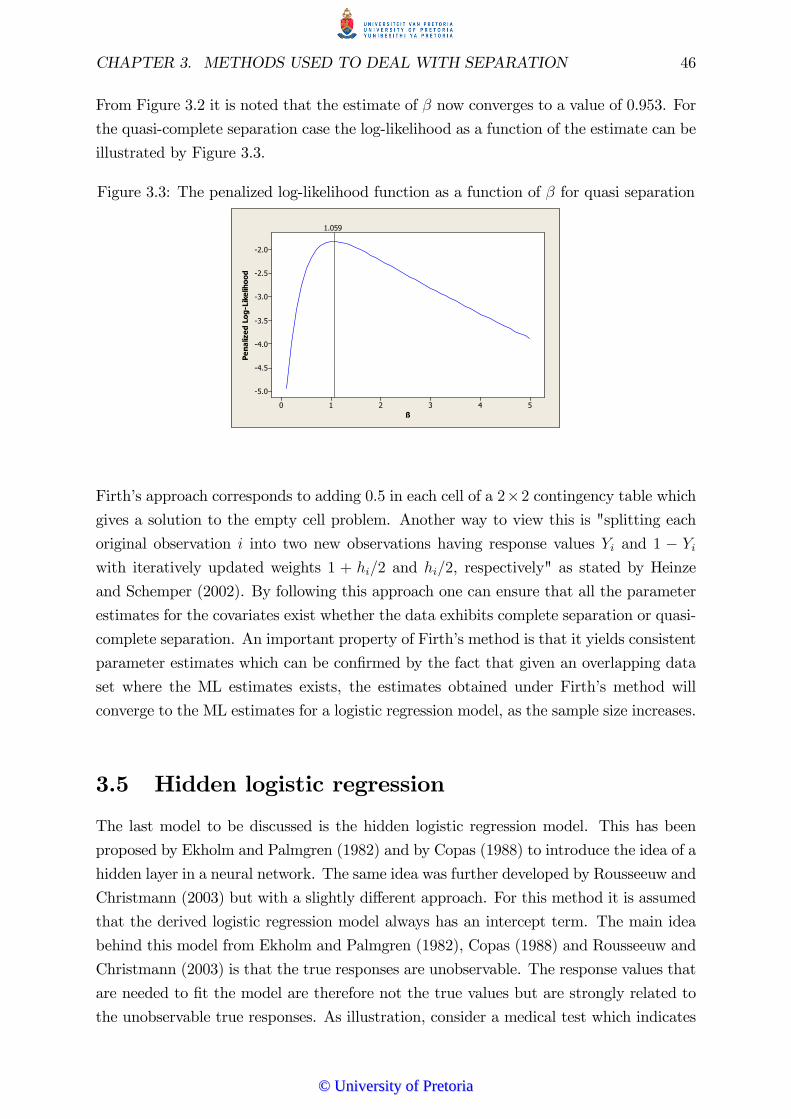
CHAPTER 3. METHODS USED TO DEAL WITH SEPARATION 46
From Figure 3.2 it is noted that the estimate of � now converges to a value of 0.953. For
the quasi-complete separation case the log-likelihood as a function of the estimate can be
illustrated by Figure 3.3.
Figure 3.3: The penalized log-likelihood function as a function of � for quasi separation
ß
Pena
lized
Log
Like
lihoo
d
543210
2.0
2.5
3.0
3.5
4.0
4.5
5.0
1.059
Firth�s approach corresponds to adding 0.5 in each cell of a 2�2 contingency table whichgives a solution to the empty cell problem. Another way to view this is "splitting each
original observation i into two new observations having response values Yi and 1 � Yiwith iteratively updated weights 1 + hi=2 and hi=2, respectively" as stated by Heinze
and Schemper (2002). By following this approach one can ensure that all the parameter
estimates for the covariates exist whether the data exhibits complete separation or quasi-
complete separation. An important property of Firth�s method is that it yields consistent
parameter estimates which can be con�rmed by the fact that given an overlapping data
set where the ML estimates exists, the estimates obtained under Firth�s method will
converge to the ML estimates for a logistic regression model, as the sample size increases.
3.5 Hidden logistic regression
The last model to be discussed is the hidden logistic regression model. This has been
proposed by Ekholm and Palmgren (1982) and by Copas (1988) to introduce the idea of a
hidden layer in a neural network. The same idea was further developed by Rousseeuw and
Christmann (2003) but with a slightly di¤erent approach. For this method it is assumed
that the derived logistic regression model always has an intercept term. The main idea
behind this model from Ekholm and Palmgren (1982), Copas (1988) and Rousseeuw and
Christmann (2003) is that the true responses are unobservable. The response values that
are needed to �t the model are therefore not the true values but are strongly related to
the unobservable true responses. As illustration, consider a medical test which indicates
©© UUnniivveerrssiittyy ooff PPrreettoorriiaa
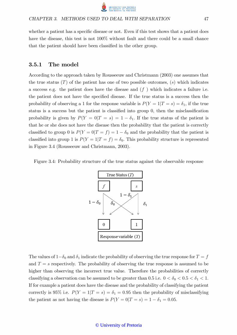
CHAPTER 3. METHODS USED TO DEAL WITH SEPARATION 47
whether a patient has a speci�c disease or not. Even if this test shows that a patient does
have the disease, this test is not 100% without fault and there could be a small chance
that the patient should have been classi�ed in the other group.
3.5.1 The model
According to the approach taken by Rousseeuw and Christmann (2003) one assumes that
the true status (T ) of the patient has one of two possible outcomes, (s) which indicates
a success e.g. the patient does have the disease and (f ) which indicates a failure i.e.
the patient does not have the speci�ed disease. If the true status is a success then the
probability of observing a 1 for the response variable is P (Y = 1jT = s) = �1, if the truestatus is a success but the patient is classi�ed into group 0, then the misclassi�cation
probability is given by P (Y = 0jT = s) = 1 � �1: If the true status of the patient isthat he or she does not have the disease then the probability that the patient is correctly
classi�ed to group 0 is P (Y = 0jT = f) = 1� �0 and the probability that the patient isclassi�ed into group 1 is P (Y = 1jT = f) = �0: This probability structure is representedin Figure 3.4 (Rousseeuw and Christmann, 2003).
Figure 3.4: Probability structure of the true status against the observable response
The values of 1��0 and �1 indicate the probability of observing the true response for T = fand T = s respectively. The probability of observing the true response is assumed to be
higher than observing the incorrect true value. Therefore the probabilities of correctly
classifying a observation can be assumed to be greater than 0.5 i.e. 0 < �0 < 0:5 < �1 < 1:
If for example a patient does have the disease and the probability of classifying the patient
correctly is 95% i.e. P (Y = 1jT = s) = �1 = 0:95 then the probability of misclassifyingthe patient as not having the disease is P (Y = 0jT = s) = 1� �1 = 0:05:
©© UUnniivveerrssiittyy ooff PPrreettoorriiaa
CHAPTER 3. METHODS USED TO DEAL WITH SEPARATION 48
3.5.2 The ML method
Since the true response is the unobservable value that needs to be estimated, an ML
estimate needs to be calculated for T . For this case as illustrated by Rousseeuw and
Christmann (2003) in Figure 3.4, the estimate for T only has one of two possibilities (since
it is a binary variable) and for each outcome there is a probability that it is correctly
classi�ed or not. If the true response is a failure (f) then the likelihood of observing
Y = 0 is greater than observing Y = 1; likewise if the true response is a success (s) the
likelihood of observing Y = 1 is greater than observing Y = 0. From this argument the
ML estimator for T , given the response (Y = y); can be expressed by
bT (Y = 0) = f (3.25)bT (Y = 1) = s:
If the observed value is assigned to group 1 i.e. Y = 1 then one of two possibilities
could have occurred, the true response is a success and was correctly classi�ed or the true
response is a failure and was misclassi�ed. Therefore the probability of an observed value
being placed into group 1 conditional on the ML estimator for T can be given by
P (Y = 1jbT ) = �0 if y = 0
�1 if y = 1(3.26)
where y is the observed value of Y: To express equation (3.26) in a single line equation,
let eY denote equation (3.26) theneY = �0 + (�1 � �0)Y = (1� Y )�0 + Y �1: (3.27)
The value for eY is a weighted average of �0 and �1 with weights of (1 � Y ) and Yrespectively.
Since logistic regression is based on n observations from a Bernoulli distribution, the
observed value for Y for the ith sample can be expressed by
eyi = (1� yi)�0 + yi�1 (3.28)
where eyi is the pseudo-observation for each individual. This pseudo-observations is adeterministic result of the observed value yi:
The resulting estimated likelihood function of the pseudo-observations eyi is given byl(�jey1; :::; eyn) = nY
i=1
� eyii (1� �i)1�eyi : (3.29)
©© UUnniivveerrssiittyy ooff PPrreettoorriiaa
CHAPTER 3. METHODS USED TO DEAL WITH SEPARATION 49
Since the true likelihood function depends on the unobservable values t1; :::; tn the like-
lihood function in equation (3.29) is only an estimation. If �0 = 0 and �1 = 1 the true
likelihood is known, therefore, since eyi is just an estimation of this value the value for eyiwill strictly lie between 0 and 1. To obtain the ML estimator for the model one can take
the natural logarithm of equation (3.29) given by
log l(�jey1; :::; eyn) = nXi=1
(eyi log �i + (1� eyi) log(1� �i)) (3.30)
and set the derivative of equation (3.30) with respect to �j; j = 1; :::;m equal to 0 i.e.
log l(�jey1; :::; eyn)@�j
=nXi=1
eyixij � nXi=1
exij�j(xij)
1 + exij�j
=
nXi=1
eyixij � nXi=1
�ixij
=nXi=1
(eyi � �i)xij set= 0: (3.31)
When only the partial derivative with respect to �0 is considered the derivative of the
log-likelihood function set equal to 0 is given by
log l(�jey1; :::; eyn)@�0
=nXi=1
eyi � nXi=1
e�0
1 + e�0
=nXi=1
eyi � nXi=1
�iset= 0: (3.32)
This leads to the result that the sum of the pseudo-observations is equivalent to the sum
of the estimated probabilities expressed by
nXi=1
eyi = nXi=1
b�i: (3.33)
Equations (3.29), (3.30), (3.31) and (3.33) are all equivalent to equation (1.11), (1.12),
(1.13) and (1.15) respectively where yi = eyi:3.5.3 Determining the values for �0 and �1be
Since the true values for a type I and type II error are rarely known in practice, in most
cases the values for �0 and �1 must be calculated from theoretical values. One approach
for di¤erent values of �0 and �1 is explained by Copas (1988) and is based on a �xed
©© UUnniivveerrssiittyy ooff PPrreettoorriiaa

CHAPTER 3. METHODS USED TO DEAL WITH SEPARATION 50
value. Since �0 is the probability of an observation being misclassi�ed into group 1 when
the actual outcome is group 0, it should be a small value. �1 is the probability of an
observation being correctly classi�ed into group 1 and therefore this is expected to be a
high value. From this information let
�0 =
�1 = 1� (3.34)
with � 0 and the value for typically ranging from 0.01 to 0.02. As shown in Copas
(1988) desirable results are obtained when = 0:01 whereas a value of = 0:05 is a too
high. This method is preferable when simplicity is required.
The method developed by Copas (1988) is most e¤ective when the data set is symmetric,
i.e. when the dependent variable has an equal number of 0 and 1�s. When an asymmetric
data set is dealt with, the approach discussed by Rousseeuw and Christmann (2003) in
Section 3.5.3 can be considered. For further discussion of the method done by Rousseeuw
and Christmann (2003) assume �i is restricted to one value for all i = 1; 2; :::; n namely �:
It is more appropriate to consider the marginal distribution of yi from which the estimate,b� can be obtained by using the number of 0�s and 1�s observed.To obtain the estimated probability of observing a success, one can argue that b� is theaverage of the pseudo observations in equation (3.33)
nXi=1
b�i =nXi=1
eyii.e.
nXi=1
b� =nXi=1
eyii.e. nb� =
nXi=1
eyii.e. b� =
1
n
nXi=1
eyi: (3.35)
By combining the results of equations (3.28), (3.33) and (3.35) the estimated probability
can be expressed (Rousseeuw and Christmann, 2003) in terms of �0 and �1:
©© UUnniivveerrssiittyy ooff PPrreettoorriiaa

CHAPTER 3. METHODS USED TO DEAL WITH SEPARATION 51
b� =1
n
nXi=1
eyi = (1� b�)�0 + b��1i.e. b� � b��1 = �0 � b��0i.e.
1� �1�1 � b� =
�0b� � �0 (3.36)
The two ratios given in equation (3.36) are both equal to a small positive number, say �;
since to it reasonable to assume
�0 < b� < �1: (3.37)
Therefore from equation (3.36) the value for �0 and �1 can be expressed in terms of b�and � by
� =1� �1�1 � b�
�(�1 � b�) = 1� �1��1 + �1 = 1 + �b��1(� + 1) = 1 + �b�
�1 =1 + �b�� + 1
(3.38)
and
� =�0b� � �0
�(b� � �0) = �0
�b� + ��0 = �0
��0 � �0 = ��b��0 =
��b�� � 1
�0 =�b�� + 1
: (3.39)
Since for this model the extreme values of 0 and 1 are not applicable to the esti-
mated probabilities, the value for b� cannot simply be the average of the observations,� = 1
n
nXi=1
yi. There has to be a constraint to ensure a value which is strictly less than 1
and strictly more than 0. One possible bound on b� is given by
©© UUnniivveerrssiittyy ooff PPrreettoorriiaa

CHAPTER 3. METHODS USED TO DEAL WITH SEPARATION 52
b� = max(�;min(1� �; �)) (3.40)
which ensures 0 < b� < 1:The ratios in equations (3.38) and (3.39) correspond with the constraint given in equation
(3.37) and the fact that 0 < b� < 1: This can be veri�ed by�1 =
1 + �b�� + 1
>b� + �b�� + 1
=b�(1 + �)� + 1
= b� (3.41)
and
�0 =�b�� + 1
<b� + �b�� + 1
=b�(1 + �)� + 1
= b�: (3.42)
The two misclassi�cation probabilities of this model is P (Y = 0jT = s) = 1 � �1 andP (Y = 1jT = f) = �0: These two values will always be smaller than the small positivenumber � as shown by
�0 =�b�� + 1
<�
� + 1< � (3.43)
and
1� �1 =1 + � � 1� �b�
� + 1=(1� b�)�1 + �
<�
1 + �< �: (3.44)
The commonly used value for � is 0:01 as advocated by Rousseeuw and Christmann
(2003). Then if a balanced data set is observed the estimated probability is given byb� = 0:5 which implies �0 = 1� �1 from equations (3.38) and (3.39). This yields the sameresults as for a symmetric data set discussed by Copas(1988) and shown by equation
(3.34).
If one considers a asymmetric data set with say 20 observations and 19 observed yi = 1,
with � = 0:01 the estimated probability from equation (3.40) is given by
b� = max
�0:01;min
�1� 0:01; 19
20
��= max(0:01;min(0:99; 0:95))
= max(0:01; 0:95)
= 0:95:
Therefore the probability of a misclassi�cation, calculated by equation (3.39), is
�0 =�b�� + 1
=0:01� 0:951:01
= 0:0094
©© UUnniivveerrssiittyy ooff PPrreettoorriiaa

CHAPTER 3. METHODS USED TO DEAL WITH SEPARATION 53
and the probability of an observation to be correctly classi�ed into group 1, from equation
(3.38), is
�1 =1 + �b�� + 1
=1 + (0:01� 0:95)
1:01= 0:9995:
For the asymmetric case this approach gives less biased estimates than for the case where
�0 and �1 are set to a �xed value.
This method has many advantages; it is robust against separation and against outliers.
Since the issue of outliers will not be examined further the interested reader is referred to
Rousseeuw and Christmann (2003) where a full discussion with examples and simulations
are given.
3.6 Conclusion
Many di¤erent solutions for complete and quasi-complete separation exist in practice.
Each method has its own bene�ts and disadvantages, which should be investigated before
applying each method. For the methods which were considered exact logistic regression
performs well with categorical covariates but caution should be applied when using this
method to a sparse data set. Firth�s method and the hidden logistic regression method
can be applied to a data set which contains both continuous and categorical covariates.
Each method behaves di¤erently with di¤erent covariate types and sample sizes; this will
be investigated using practical applications in part II.
©© UUnniivveerrssiittyy ooff PPrreettoorriiaa

Part II
Practical Application
54
©© UUnniivveerrssiittyy ooff PPrreettoorriiaa
Chapter 4
Overview/ Outline of Part II
In part I the theory of logistic regression is summarised and the problem of complete and
quasi-complete separation was identi�ed in Chapter 2 of part I. Three di¤erent methods
to use when either complete or quasi-complete separation is present were discussed in
Chapter 3 of part I. The three di¤erent methods mentioned can however not always
be applied to any given data set to predict a binary outcome. Keeping this in mind
Chapter 5 will investigate a small sample of twenty observations which exhibits complete
separation. To study di¤erent types of independent variables the �rst example will include
only continuous covariates, the second both continuous and categorical covariates and the
�nal example of Chapter 5 will investigate the case where only categorical covariates are
used to predict a binary outcome. In Chapter 6 a large sample with only categorical
covariates will be investigated.
For each of the di¤erent combinations of covariate types mentioned, the general logis-
tic regression model will be investigated to con�rm if complete separation is present.
From SAS, PROC LOGISTIC, it is con�rmed that all the examples of Chapter 5 exhibit
complete separation and in Chapter 6 exhibit quasi-complete separation, but for the case
where the computer packages mentioned in Section 2.5 are not available a few exploratory
methods can be considered. First a scatter plot of the categorical covariates (which is
obtained with MINITAB) will be introduced from which one can visually con�rm if there
is a split between the groups or not. Secondly by considering numerical analysis it can
be examined whether the coe¢ cient estimates converges and if the standard error of the
coe¢ cient estimates tends to in�nity as the number of iterations increase or not, ob-
tained by both SAS and MINITAB. Once the coe¢ cient estimates are obtained it can be
con�rmed with the Wald and LR test statistic (obtained from SAS) if b� is signi�cantlydi¤erent from 0 or not.
All the covariates which are considered for each model are signi�cant in predicting the
dichotomous outcome of that example. All interactions between the covariates were also
originally included in the model. The �nal models given in equations (5.1), (5.2) and
55
©© UUnniivveerrssiittyy ooff PPrreettoorriiaa

CHAPTER 4. OVERVIEW/ OUTLINE OF PART II 56
(5.3) are obtained from only choosing the signi�cant covariates to predict the outcome
according to forward stepwise logistic regression in SPSS.
For each of the di¤erent independent variable types mentioned (continuous and cate-
gorical) three methods will be applied, namely; exact logistic regression, Firth�s method
and �nally hidden logistic regression. Once parameter estimates are obtained for each
of these methods one needs to test if the coe¢ cient estimates are signi�cant or not. For
exact logistic regression and Firth�s method the coe¢ cient estimates with the appropriate
signi�cance level are calculated with SAS. The two-sided conditional exact test is used to
test the signi�cance of the coe¢ cients obtained under exact logistic regression whereas
Wald�s test statistic is used for the coe¢ cients obtained under Firth�s method. For hid-
den logistic regression the R program code given in Appendix G is applied to obtain the
coe¢ cient estimates and the appropriate signi�cance levels since there is no procedure
available in SAS as of yet to calculate these values. The Wald test statistic is also used
to calculate the signi�cance of the coe¢ cient estimates.
After testing the signi�cance of the individual coe¢ cient estimates, the overall validity
of the model needs to be examined. Some of the goodness-of-�t measures mentioned
in Section 1.10 will be considered namely the Pearson chi-square, deviance, Hosmer-
Lemeshow tests and �nally the classi�cation table. For the classi�cation tables, the
rows represent the observed values and the columns represent the predicted value for
the speci�ed model. All the examples will make use of only two covariates to compare
the di¤erent approaches on the same number of observations. Therefore none of the
model �t statistics discussed in Section 1.10.3 will be necessary, as these tests are used to
compare models with di¤erent number of covariates to each other. To calculate the formal
goodness-of-�t test statistics a SAS, PROC IML code is available in Appendix F and H
for the classi�cation tables and Pearson chi-square, deviance and Hosmer-Lemeshow tests
respectively. This has been done since the mentioned goodness-of-�t test statistics are
not available for exact or hidden logistic regression in SAS. From the goodness-of-�t
statistics it can be concluded if the method considered is a good choice for that speci�c
combination of covariates.
For the small sample case one should keep in mind that the Wald, LR, Pearson chi-
square and deviance test statistics all depend on the assumption of an approximate chi-
square distribution and could therefore give misleading results. When the statistics give
con�icting results it could be a sign that the large-sample approximation is unreliable.
Also, the Pearson chi-square and deviance test statistic are most reliable when considering
a data set with only categorical observations. The numerical values for the Pearson chi-
square and the deviance test statistic should be close to each other in value as stated in
Collett (2003, p. 87): "Large di¤erences between the two statistics can be taken as an
©© UUnniivveerrssiittyy ooff PPrreettoorriiaa

CHAPTER 4. OVERVIEW/ OUTLINE OF PART II 57
indication that the chi-squared approximation to the distribution of the deviance or the
X2-statistic is not adequate."
When considering the Hosmer-Lemeshow test, as explained by Xie et al. (2008), it has
been shown that when the number of groups are few this test statistic almost always
shows that the model is adequate and therefore when possible only consider the test
statistic for a large number of groups.
©© UUnniivveerrssiittyy ooff PPrreettoorriiaa

Chapter 5
Complete separation (small sample)
5.1 Introduction
Complete and quasi-complete separation is most likely to occur in small data sets which
typically occur in medical sciences as discussed in Heinze (2006), in economic indices as
shown in Beggs et al. (1981) and even in marketing as indicated in Chapman (1984).
The most common occurrence of complete or quasi-complete separation is found in bio-
statistics (medical sciences) where the application of a clinical trial usually demands a
dichotomous outcome (if a patient survived or died, if a treatment worked or did not
work, etc.) and since most medical test are typically expensive, a clinical trial will most
likely consist of a small sample.
To compare the di¤erent approaches mentioned in Chapter 3, three di¤erent data sets will
be considered. The three data sets will be identical in size (n = 20) and all of them will
be balanced, i.e. yi = 1 for 10 observations and yi = 0 for the remaining 10 observations.
Each of the three examples exhibit complete separation and will have two covariates to
predict a dichotomous outcome.
The �rst clinical trial from Philippeos et. al (2009) is used to predict whether a pa-
tient is HIV positive or HIV negative based on two continuous covariates (NMR-based
metabonomics).
The second example from Haberman (1973) is based on a sample which consists of a
combination of a categorical covariate (age group of a patient) and a continuous covariate
(number of positive axillary nodes detected) to predict if a patient survived or died within
5 years of receiving a breast cancer operation .
Finally the third example is a sample acquired from Kaggle (2012); this data set predicts
whether a passenger who was Section the RMS Titanic survived or died based on two
categorical covariates, the class of the passenger (�rst class, second class or third class)
and the sex of the passenger (female or male).
58
©© UUnniivveerrssiittyy ooff PPrreettoorriiaa

CHAPTER 5. COMPLETE SEPARATION (SMALL SAMPLE) 59
5.2 Continuous covariates
5.2.1 HIV status example
Consider the data set: HIV Status (Appendix A) which was supplied by Prof. D. Meyer.
This data set consists of high-resolution proton NMR (1H-NMR) spectroscopic pro�ling
of biological �uids; these metabonomics have contributed to the identi�cation and study
of human disease. In Philippeos, Ste¤ens and Meyer (2009) these metabonomics are
speci�cally applied to identify whether a patient is HIV negative or HIV positive.
This experiment involves 20 patients of whom 10 is HIV negative (HIV�; yi = 1) and 10
of the patients are HIV positive and currently on anti-retroviral therapy (HIV+; yi = 0).
From the initial data set, 88 covariates where obtained from the NMR instrument from
which only 2 were signi�cant, xV 3:74 and xV 1:18. Both the covariates xV 3:74 and xV 1:18are continuous and complete separation is found within this data set which can also be
con�rmed by the scatterplot in Figure 5.1. xV 3:74 and xV 1:18 are shown in Figure 5.1 and
the groups are indicated for yi = 1 and yi = 0:
Figure 5.1: Scatter plot of xV 3:74 vs. xV 1:18 grouped according to the observed value of y:
V1.18
V3.7
4
2.42.11.81.51.2
0.0
0.1
0.2
0.3
0.4
0.5
2.42.11.81.51.20 1 HIV
Status01
Panel variable: HIV Status0 HIV Positive 1 HIV Negative
Since this data set consists of only continuous covariates, it is a sparse data set which is
con�rmed by the fact that there are only two observations that share the same covariate
pattern therefore there are 19 unique covariate patterns i.e. q = 19.
5.2.2 General logistic regression model
Since this data set consists of continuous covariates, no dummy variables are required to
formulate a logistic regression model. The equation for a logistic regression model applied
to the HIV status data set is given by equation (5.1).
logit(�i) = �0 + �v3:74xV 3:74 + �v1:18xV 1:18 (5.1)
©© UUnniivveerrssiittyy ooff PPrreettoorriiaa

CHAPTER 5. COMPLETE SEPARATION (SMALL SAMPLE) 60
The e¤ect of the interaction between xV 3:74 and xV 1:18 is not signi�cant and therefore
not included in the model. From the SAS, PROC LOGISTIC, procedure the coe¢ cient
estimates for equation (5.1) after 8 iterations are found as shown by the �rst column of
Table 5.1.
Table 5.1: Logistic regression coe¢ cient estimates for HIV status
After 8 iterations After 25 iterations After 100 iterationsVariable b� SE of b� b� SE of b� b� SE of b�Intercept 10.6243 70.4261 45.6032 184766 96.0844 761609xV 3:74 -160.8 272.3 -611.284 731383 -1068.22 3662281xV 1:18 -39.7412 74.3653 -153.135 180033 -269.342 559114
From the output it is noticed that the standard error for all coe¢ cients estimates are
considerably greater than the corresponding coe¢ cient estimates. This is the �rst indica-
tion that the coe¢ cient estimates should be evaluated with care. Even though estimated
values for the coe¢ cients are obtained, there is a warning given by the program that
the values haven�t converged and that the validity of the model is questionable. To test
the validity of the coe¢ cient estimates after 8 iterations the LR and Wald statistic, with
corresponding p-values, is given in Table 5.2 calculated by equations (1.41) and (1.47)
respectively.
Table 5.2: LR and Wald statistics for HIV statusAfter 8 iterations
Variable Statistic p-valueLR 10:6243 < 0:0001Wald 70:4261 0:8398
Under the null hypothesis that � is not signi�cantly di¤erent from 0, the LR statistic
rejects the null hypothesis and the Wald statistic does not reject the null hypothesis.
The two con�icting conclusions of the LR and Wald statistics are an indication that an
approximate chi-square distribution wasn�t obtained. This is due to the small sample
of 20 observations which is used. The maximum number of iterations were increased to
25 and 100 respectively. The results for the coe¢ cient estimates and standard error in
Table 5.1 of the coe¢ cient estimates (obtained in MINITAB) are given columns 2 and 3
respectively. From these results it is clear that the parameter estimates increase as the
log-likelihood function increases (as indicated by Figure 2.2). As the number of iterations
increases, the value for b� and the standard error for b� increase and tend to in�nity sincethere is no convergence. This indicates that none of the coe¢ cient estimates found in
Table 5.1 are reliable and other methods should be applied.
©© UUnniivveerrssiittyy ooff PPrreettoorriiaa
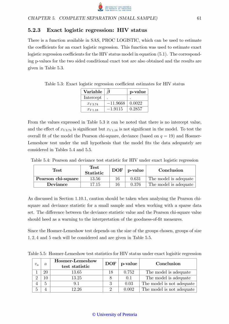
CHAPTER 5. COMPLETE SEPARATION (SMALL SAMPLE) 61
5.2.3 Exact logistic regression: HIV status
There is a function available in SAS, PROC LOGISTIC, which can be used to estimate
the coe¢ cients for an exact logistic regression. This function was used to estimate exact
logistic regression coe¢ cients for the HIV status model in equation (5.1). The correspond-
ing p-values for the two sided conditional exact test are also obtained and the results are
given in Table 5.3.
Table 5.3: Exact logistic regression coe¢ cient estimates for HIV status
Variable b� p-valueIntercept : .xV 3:74 �11:9668 0:0022xV 1:18 �1:9115 0:2857
From the values expressed in Table 5.3 it can be noted that there is no intercept value,
and the e¤ect of xV 3:74 is signi�cant but xV 1:18 is not signi�cant in the model. To test the
overall �t of the model the Pearson chi-square, deviance (based on q = 19) and Hosmer-
Lemeshow test under the null hypothesis that the model �ts the data adequately are
considered in Tables 5.4 and 5.5.
Table 5.4: Pearson and deviance test statistic for HIV under exact logistic regression
TestTest
Statistic DOF p-value Conclusion
Pearson chi-square 13:56 16 0:631 The model is adequateDeviance 17:15 16 0:376 The model is adequate
As discussed in Section 1.10.1, caution should be taken when analysing the Pearson chi-
square and deviance statistic for a small sample and when working with a sparse data
set. The di¤erence between the deviance statistic value and the Pearson chi-square value
should heed as a warning to the interpretation of the goodness-of-�t measures.
Since the Hosmer-Lemeshow test depends on the size of the groups chosen, groups of size
1; 2; 4 and 5 each will be considered and are given in Table 5.5.
Table 5.5: Hosmer-Lemeshow test statistics for HIV status under exact logisitic regression
va aHosmer-Lemeshow
test statistic DOF p-value Conclusion
1 20 13:65 18 0:752 The model is adequate2 10 13:25 8 0:1 The model is adequate4 5 9:1 3 0:03 The model is not adequate5 4 12:26 2 0:002 The model is not adequate
©© UUnniivveerrssiittyy ooff PPrreettoorriiaa

CHAPTER 5. COMPLETE SEPARATION (SMALL SAMPLE) 62
Hosmer-Lemeshow�s p-values for 4 and 5 groups, of size 5 and 4 respectively, are the
lowest and the null hypothesis that the model is an adequate model is rejected. For 1
group of size 20 and 2 groups of size 10 each the p-values are greater than 0:05 and the
null hypothesis is not rejected at a signi�cance level of � = 0:05. Over the di¤erent group
sizes the p-values vary between 0:002 and 0:752 which is a clear indication that the group
size used makes a di¤erence with this test. From the Pearson chi-square and deviance
test the model is adequate. From the Hosmer-Lemeshow statistics the indication is that
the model is not adequate since the results for a larger number of groups (va = 4 and
va = 5) are more reliable than for a few number of groups, and these indicate it is not a
good model.
Finally consider the classi�cation table for the exact logistic regression model with dif-
ferent cut-o¤ values for the predicted probability. The cut-o¤ values ranges from b� = 0:1to b� = 0:9 in increments of 0.1. To illustrate how well the predicted model performs
with the di¤erent cut-o¤ levels the following classi�cation tables are given (Tables 5.6
and 5.7).
Table 5.6: Classi�cation table for HIV status under exact logisitic regression for a cut-o¤probability from 0.1 to 0.5.
Exactb� Predictedvalues
Percentagecorrect
HIV� HIV+
0:1 Observed HIV� 10 0 100%Values HIV+ 10 0 0%overall%
50%
0:2 Observed HIV� 10 0 100%to Values HIV+ 8 2 20%
0:4overall%
60%
0:5 Observed HIV� 10 0 100%Values HIV+ 6 4 40%overall%
70%
©© UUnniivveerrssiittyy ooff PPrreettoorriiaa

CHAPTER 5. COMPLETE SEPARATION (SMALL SAMPLE) 63
Table 5.7: Classi�cation table for HIV status under exact logisitic regression for a cut-o¤probability from 0.6 to 0.9.
Exactb� Predictedvalues
Percentagecorrect
HIV� HIV+
0:6 Observed HIV� 10 0 100%Values HIV+ 2 8 80%overall%
90%
0:7 Observed HIV� 10 0 100%Values HIV+ 1 9 90%overall%
95%
0:8 Observed HIV� 10 0 100%Values HIV+ 0 10 100%overall%
100%
0:9 Observed HIV� 3 7 30%Values HIV+ 0 10 100%overall%
65%
From Table 5.7 it can be noted that the exact logistic regression model classi�es the
values well for a cut-o¤ value between 0.6 and 0.8. Since this is a balanced data set, the
classi�cation for b� = 0:5 will be used in practice and for this cut-o¤ value the number ofobservations which are correctly classi�ed is 14=20 = 70% from Table 5.6.
Overall the exact logistic regression model only has one signi�cant parameter, is indicated
as an overall good �t by Pearson chi-square and deviance tests, but not by the Hosmer-
Lemeshow test. Finally this model has a relatively good classi�cation rate.
5.2.4 Firth�s Method: HIV status
Continuing with the HIV status example SAS, PROC LOGISTIC, will once again be
applied with the model statement ��rth�. The coe¢ cient estimates for the HIV status
data set under Firth�s model are given in Table 5.8 and the estimates converged after 5
iterations.
It can be noted from Table 5.8 that the parameter estimates for both xV 3:74 and xV 1:18are signi�cant at a 5% level (p-values obtained from Wald statistic discussed in Section
1.11.1). Even though the covariates used are signi�cant it is empirical to test the overall
performance of the model (given Firth�s coe¢ cient estimates). For overall goodness-of-�t
©© UUnniivveerrssiittyy ooff PPrreettoorriiaa
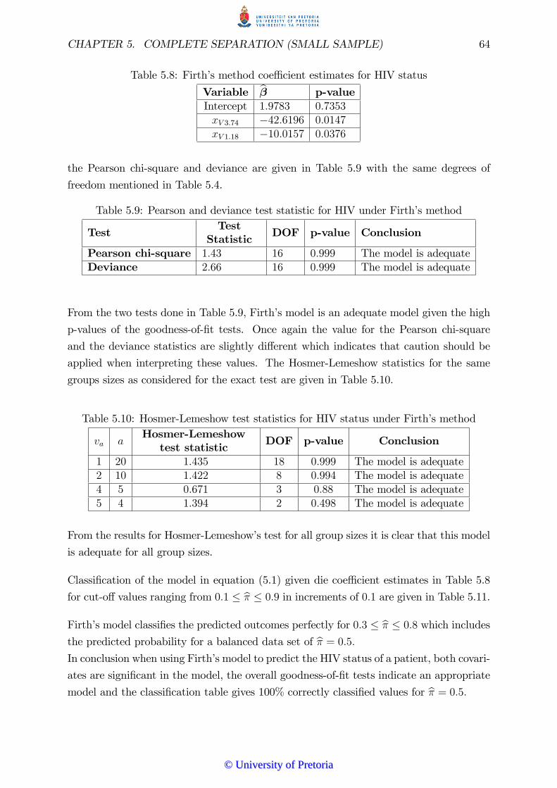
CHAPTER 5. COMPLETE SEPARATION (SMALL SAMPLE) 64
Table 5.8: Firth�s method coe¢ cient estimates for HIV status
Variable b� p-valueIntercept 1:9783 0:7353xV 3:74 �42:6196 0:0147xV 1:18 �10:0157 0:0376
the Pearson chi-square and deviance are given in Table 5.9 with the same degrees of
freedom mentioned in Table 5.4.
Table 5.9: Pearson and deviance test statistic for HIV under Firth�s method
TestTest
Statistic DOF p-value Conclusion
Pearson chi-square 1:43 16 0:999 The model is adequateDeviance 2:66 16 0:999 The model is adequate
From the two tests done in Table 5.9, Firth�s model is an adequate model given the high
p-values of the goodness-of-�t tests. Once again the value for the Pearson chi-square
and the deviance statistics are slightly di¤erent which indicates that caution should be
applied when interpreting these values. The Hosmer-Lemeshow statistics for the same
groups sizes as considered for the exact test are given in Table 5.10.
Table 5.10: Hosmer-Lemeshow test statistics for HIV status under Firth�s method
va aHosmer-Lemeshow
test statistic DOF p-value Conclusion
1 20 1:435 18 0:999 The model is adequate2 10 1:422 8 0:994 The model is adequate4 5 0:671 3 0:88 The model is adequate5 4 1:394 2 0:498 The model is adequate
From the results for Hosmer-Lemeshow�s test for all group sizes it is clear that this model
is adequate for all group sizes.
Classi�cation of the model in equation (5.1) given die coe¢ cient estimates in Table 5.8
for cut-o¤ values ranging from 0:1 � b� � 0:9 in increments of 0:1 are given in Table 5.11.Firth�s model classi�es the predicted outcomes perfectly for 0:3 � b� � 0:8 which includesthe predicted probability for a balanced data set of b� = 0:5:In conclusion when using Firth�s model to predict the HIV status of a patient, both covari-
ates are signi�cant in the model, the overall goodness-of-�t tests indicate an appropriate
model and the classi�cation table gives 100% correctly classi�ed values for b� = 0:5:
©© UUnniivveerrssiittyy ooff PPrreettoorriiaa

CHAPTER 5. COMPLETE SEPARATION (SMALL SAMPLE) 65
Table 5.11: Classi�cation table for HIV status under Firth�s method for cut-o¤probabilityfrom 0.1 to 0.9
Firthb� Predictedvalues
Percentagecorrect
HIV� HIV+
0:1 Observed HIV� 10 0 100%Values HIV+ 3 7 70%overall%
85%
0:2 Observed HIV� 10 0 100%Values HIV+ 1 9 90%overall%
95%
0:3 Observed HIV� 10 0 100%to Values HIV+ 0 10 100%
0:8overall%
100%
0:9 Observed HIV� 8 2 80%Values HIV+ 0 10 100%overall%
90%
5.2.5 Hidden logistic regression model
The �nal approach, and most recently developed model, to deal with completely separated
data is a hidden logistic regression model. The coe¢ cient estimates for the HIV data set
based on a hidden logistic regression model obtained with the R program in Appendix
G (mentioned in the overview of part II) are given in Table 5.12. The appropriate Wald
statistic p-values are also given in Table 5.12 next to each applicable coe¢ cient estimate.
Table 5.12: Hidden logistic regression coe¢ cient estimates for HIV status
Variable b� p-valueIntercept 5:398 0:6944xV 3:74 �82:638 0:0985xV 1:18 �20:447 0:1351
The log-likelihood function converged after 10 iterations and �nite coe¢ cient estimates
were obtained. From the values in Table 5.12 it can be noted that both the coe¢ cient
estimates for xV 3:74 and xV 1:18 are not signi�cant at a signi�cance level of � = 0:05. The
goodness-of-�t statistics for the hidden logistic regression model are given in Tables 5.13
and 5.14 for the same degrees of freedom considered for both exact logistic regression and
Firth�s model.
©© UUnniivveerrssiittyy ooff PPrreettoorriiaa

CHAPTER 5. COMPLETE SEPARATION (SMALL SAMPLE) 66
Table 5.13: Pearson and deviance test statistic for HIV under hidden logistic regression
TestTest
Statistic DOF p-value Conclusion
Pearson chi-square 0:211 16 0:999 The model is adequateDeviance 0:414 16 0:999 The model is adequate
Table 5.14: Hosmer-Lemeshow test statistics for HIV status under hidden logisitic re-gression
va aHosmer-Lemeshow
test statistic DOF p-value Conclusion
1 20 0:211 18 0:999 The model is adequate2 10 0:21 8 0:999 The model is adequate4 5 0:059 3 0:996 The model is adequate5 4 0:21 2 0:902 The model is adequate
All the goodness-of-�t tests done on the hidden logistic regression model indicate that
it is a very good model. The classi�cation of the predicted outcomes from the hidden
logistic regression model is 100% correctly classi�ed for all pre-de�ned cut-o¤ values as
shown in Table 5.15.
Table 5.15: Classi�cation table for HIV status under hidden logistic regression for cut-o¤probability from 0.1 to 0.9
Hidden logistic regressionb� Predictedvalues
Percentagecorrect
HIV� HIV+
0:1 Observed HIV� 10 0 100%to Values HIV+ 0 10 100%
0:9overall%
100%
Overall for the hidden logistic regression model even though none of the coe¢ cient esti-
mates are signi�cant, the goodness-of-�t tests and the classi�cation table indicates it is
a good model for the HIV data set.
5.2.6 Conclusion: HIV status example
From the example shown above, it can be noted that even though Firth�s method and
the hidden logistic regression model both give 100% correctly classi�ed values at b� = 0:5,only the model obtained under Firth�s method give signi�cant coe¢ cient estimates for
both xV 3:74 and xV 1:18: Since the values for b� for Firth�s method are signi�cant predictors
©© UUnniivveerrssiittyy ooff PPrreettoorriiaa

CHAPTER 5. COMPLETE SEPARATION (SMALL SAMPLE) 67
in the model it can be interpreted with more con�dence than those obtained under the
hidden logistic regression model.
The results obtained for the goodness-of-�t tests and classi�cation tables can be explained
by interpreting the predicted probabilities obtained under each model. The predicted
probabilities for each observation for exact logistic regression, Firth�s model and hidden
logistic regression are plotted in Figure 5.2.
Figure 5.2: HIV example predicted probabilities for exact, Firth and hidden
observations
Pred
icte
dpr
obab
ilitie
s
20151050
1.0
0.8
0.6
0.4
0.2
0.0
0.5
Variable
FirthHLR
yExact
The curve obtained from the predicted probabilities under the exact logistic regression
model does not resemble the curve of either the original data set or that of a logistic curve
(Figure 1.1). This explains the fact why the exact logistic regression model did not give
signi�cant coe¢ cient estimates nor was it an appropriate model according to the Hosmer
Lemeshow goodness-of-�t tests.
Firth�s model however gives a smoother curve between yi = 0 and yi = 1 which enables
a better prediction for 0 < yi < 1: The coe¢ cient estimates for Firth�s model are all
signi�cant this implies the estimated values obtained from the model can be interpreted
with more con�dence for all values of yi as seen from Figure 5.2.
Finally from Figure 5.2 the good results obtained from the goodness-of-�t tests and
the classi�cation table for hidden logistic regression can be explained. The predicted
probabilities obtained under the hidden logistic regression model closely resemble that of
the original completely separated data set. Where the hidden logistic regression model
yields predicted values close to 0 and 1, Firth�s model gave a more even distribution
of the predicted probabilities between 0 and 1, resembling Figure 1.1. Therefore the
good results for both the goodness-of-�t tests and the classi�cation table under a hidden
logistic regression model can be explained by the fact that it closely resembles the original
data set and this also explains why the coe¢ cient estimates are not signi�cant since this
model this closely resembles a data set which is separated between yi = 0 and yi = 1:
©© UUnniivveerrssiittyy ooff PPrreettoorriiaa
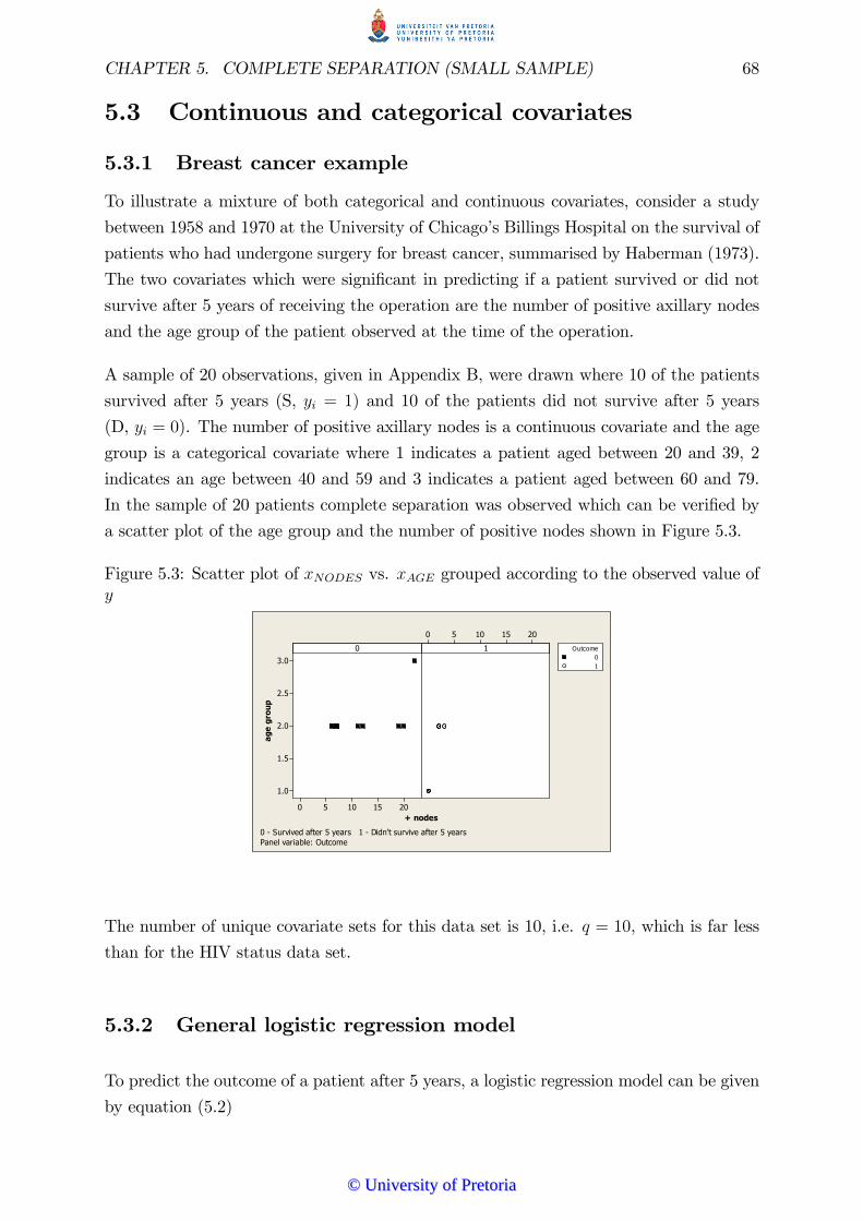
CHAPTER 5. COMPLETE SEPARATION (SMALL SAMPLE) 68
5.3 Continuous and categorical covariates
5.3.1 Breast cancer example
To illustrate a mixture of both categorical and continuous covariates, consider a study
between 1958 and 1970 at the University of Chicago�s Billings Hospital on the survival of
patients who had undergone surgery for breast cancer, summarised by Haberman (1973).
The two covariates which were signi�cant in predicting if a patient survived or did not
survive after 5 years of receiving the operation are the number of positive axillary nodes
and the age group of the patient observed at the time of the operation.
A sample of 20 observations, given in Appendix B, were drawn where 10 of the patients
survived after 5 years (S, yi = 1) and 10 of the patients did not survive after 5 years
(D, yi = 0). The number of positive axillary nodes is a continuous covariate and the age
group is a categorical covariate where 1 indicates a patient aged between 20 and 39, 2
indicates an age between 40 and 59 and 3 indicates a patient aged between 60 and 79.
In the sample of 20 patients complete separation was observed which can be veri�ed by
a scatter plot of the age group and the number of positive nodes shown in Figure 5.3.
Figure 5.3: Scatter plot of xNODES vs. xAGE grouped according to the observed value ofy
+ nodes
age
grou
p
20151050
3.0
2.5
2.0
1.5
1.0
201510500 1 Outcome
01
Panel variable: Outcome0 Survived after 5 years 1 Didn't survive after 5 years
The number of unique covariate sets for this data set is 10, i.e. q = 10, which is far less
than for the HIV status data set.
5.3.2 General logistic regression model
To predict the outcome of a patient after 5 years, a logistic regression model can be given
by equation (5.2)
©© UUnniivveerrssiittyy ooff PPrreettoorriiaa

CHAPTER 5. COMPLETE SEPARATION (SMALL SAMPLE) 69
logit(�i) = �0 + �d11xd11 + �d12xd12 + �NODESxNODES (5.2)
where the indicators of age are summarised in Table 5.16.
Table 5.16: Coding for age groups
Indicatorxd11 xd12
Group 1 (20-39 1 0Age Group 2 (40-59) 0 1
Group 3 (60-79) 0 0
The interaction between the number of positive nodes detected and the age group are
not signi�cant in predicting the survival status of a patient after 5 years and is therefore
not included in the model.
From SAS, PROC LOGISTIC, the coe¢ cient estimates for equation (5.2) did not converge
after 8 iterations. Since complete separation is present in the data set the log-likelihood
function was unable to converge even after 100 iterations, the results of the coe¢ cient
estimates are given in Table 5.17. The standard error for each coe¢ cient estimate ob-
tained after 8 iterations is greater than the coe¢ cient estimate itself, this is an indication
of unreliable coe¢ cient estimates.
Table 5.17: Logistic regression coe¢ cient estimates for breast cancer
After 8 iterations After 25 iterations After 100 iterationsVariable b� SE of b� b� SE of b� b� SE of b�Intercept 77:67 168:7 �289:96 457849 �251:769 652712xd11 �68:47 175:9 263:75 481327 192:486 500000xd12 �59:8 146:8 222:63 448157 160:788 452226
xNODES �3:95 6:1879 14:941 14654 21:3304 41523
Subsequently as the coe¢ cient estimates did not converge, the signi�cance of the para-
meters are questionable. To test the signi�cance of vector b�;consider the LR and Waldstatistic given in Table 5.18.
Table 5.18: LR and Wald statistics for breast cancerAfter 8 iterations
Variable Test statistic value p-valueLR 27:7 < 0:0001Wald 0:4516 0:93
Under the null hypothesis that � does not signi�cantly di¤er from 0, for the coe¢ cient
estimates obtained after 8 iterations, it can be noted that the according to the LR test
©© UUnniivveerrssiittyy ooff PPrreettoorriiaa
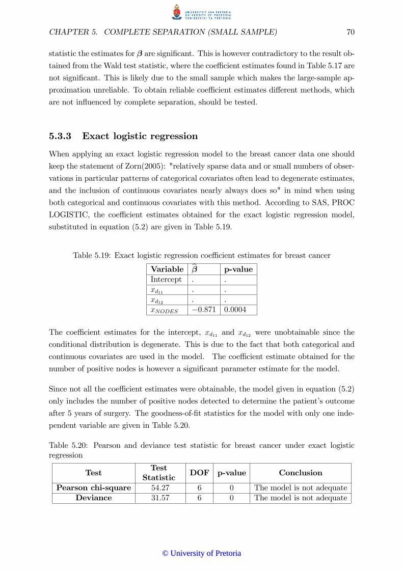
CHAPTER 5. COMPLETE SEPARATION (SMALL SAMPLE) 70
statistic the estimates for � are signi�cant. This is however contradictory to the result ob-
tained from the Wald test statistic, where the coe¢ cient estimates found in Table 5.17 are
not signi�cant. This is likely due to the small sample which makes the large-sample ap-
proximation unreliable. To obtain reliable coe¢ cient estimates di¤erent methods, which
are not in�uenced by complete separation, should be tested.
5.3.3 Exact logistic regression
When applying an exact logistic regression model to the breast cancer data one should
keep the statement of Zorn(2005): "relatively sparse data and or small numbers of obser-
vations in particular patterns of categorical covariates often lead to degenerate estimates,
and the inclusion of continuous covariates nearly always does so" in mind when using
both categorical and continuous covariates with this method. According to SAS, PROC
LOGISTIC, the coe¢ cient estimates obtained for the exact logistic regression model,
substituted in equation (5.2) are given in Table 5.19.
Table 5.19: Exact logistic regression coe¢ cient estimates for breast cancer
Variable b� p-valueIntercept . .xd11 . .xd12 . .xNODES �0:871 0:0004
The coe¢ cient estimates for the intercept, xd11 and xd12 were unobtainable since the
conditional distribution is degenerate. This is due to the fact that both categorical and
continuous covariates are used in the model. The coe¢ cient estimate obtained for the
number of positive nodes is however a signi�cant parameter estimate for the model.
Since not all the coe¢ cient estimates were obtainable, the model given in equation (5.2)
only includes the number of positive nodes detected to determine the patient�s outcome
after 5 years of surgery. The goodness-of-�t statistics for the model with only one inde-
pendent variable are given in Table 5.20.
Table 5.20: Pearson and deviance test statistic for breast cancer under exact logisticregression
TestTest
Statistic DOF p-value Conclusion
Pearson chi-square 54:27 6 0 The model is not adequateDeviance 31:57 6 0 The model is not adequate
©© UUnniivveerrssiittyy ooff PPrreettoorriiaa
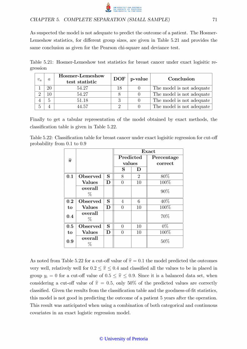
CHAPTER 5. COMPLETE SEPARATION (SMALL SAMPLE) 71
As suspected the model is not adequate to predict the outcome of a patient. The Hosmer-
Lemeshow statistics, for di¤erent group sizes, are given in Table 5.21 and provides the
same conclusion as given for the Pearson chi-square and deviance test.
Table 5.21: Hosmer-Lemeshow test statistics for breast cancer under exact logisitic re-gression
va aHosmer-Lemeshow
test statistic DOF p-value Conclusion
1 20 54:27 18 0 The model is not adequate2 10 54:27 8 0 The model is not adequate4 5 51:18 3 0 The model is not adequate5 4 44:57 2 0 The model is not adequate
Finally to get a tabular representation of the model obtained by exact methods, the
classi�cation table is given in Table 5.22.
Table 5.22: Classi�cation table for breast cancer under exact logisitic regression for cut-o¤probability from 0.1 to 0.9
Exactb� Predictedvalues
Percentagecorrect
S D0:1 Observed S 8 2 80%
Values D 0 10 100%overall%
90%
0:2 Observed S 4 6 40%to Values D 0 10 100%
0:4overall%
70%
0:5 Observed S 0 10 0%to Values D 0 10 100%
0:9overall%
50%
As noted from Table 5.22 for a cut-o¤ value of b� = 0:1 the model predicted the outcomesvery well, relatively well for 0:2 � b� � 0:4 and classi�ed all the values to be in placed ingroup yi = 0 for a cut-o¤ value of 0:5 � b� � 0:9: Since it is a balanced data set, whenconsidering a cut-o¤ value of b� = 0:5; only 50% of the predicted values are correctly
classi�ed. Given the results from the classi�cation table and the goodness-of-�t statistics,
this model is not good in predicting the outcome of a patient 5 years after the operation.
This result was anticipated when using a combination of both categorical and continuous
covariates in an exact logistic regression model.
©© UUnniivveerrssiittyy ooff PPrreettoorriiaa

CHAPTER 5. COMPLETE SEPARATION (SMALL SAMPLE) 72
5.3.4 Firth�s method
Since Firth�s method is based on penalising the existing log-likelihood function, the type
of covariates used should not have an e¤ect on the signi�cance of the model. Given the
Firth speci�cation in SAS, PROC LOGISTIC, the coe¢ cient estimates for the covariates
identi�ed in equation (5.2) are given in Table 5.23.
Table 5.23: Firth�s method coe¢ cient estimates for breast cancer
Variable b� p-valueIntercept 23:2419 0:0375xd11 �21:0352 0:0626xd12 �18:4047 0:0420
xNODES �1:0605 0:0338
Most of the coe¢ cient estimates given in Table 5.23 are signi�cant at a 5% signi�cance
level. When considering � = 0:05, xd11 is not signi�cant but since xd11 and xd12 represents
the age group together one either needs to keep or exclude both from the model. The
goodness-of-�t tests for Pearson chi-square and deviance test statistics are given in Table
5.24 followed by the Hosmer-Lemeshow�s test statistics in Table 5.25. All the goodness-
of-�t tests indicate that Firth�s model is a good model to predict the outcome of a breast
cancer patient after 5 years of surgery.
Table 5.24: Pearson and deviance test statistic for breast cancer under Firth�s method
TestTest
Statistic DOF p-value Conclusion
Pearson chi-square 2:66 6 0:85 The model is adequateDeviance 4:57 6 0:6 The model is adequate
Table 5.25: Hosmer-Lemeshow test statistics for breast cancer under Firth�s method
va aHosmer-Lemeshow
test statistic DOF p-value Conclusion
1 20 2:66 18 0:999 The model is adequate2 10 2:5 8 0:96 The model is adequate4 5 1:25 3 0:74 The model is adequate5 4 2:36 2 0:31 The model is adequate
Even though Firth�s model is an adequate model by the goodness-of-�t statistics, it is
also necessary to compare the predicted values to the actual values for a small sample.
Therefore the classi�cation table of the model with the coe¢ cients given in Table 5.23 is
given in Table 5.26.
©© UUnniivveerrssiittyy ooff PPrreettoorriiaa

CHAPTER 5. COMPLETE SEPARATION (SMALL SAMPLE) 73
Table 5.26: Classi�cation table for breast cancer under Firth�s method for cut-o¤ proba-bility from 0.1 to 0.9
Firthb� Predictedvalues
Percentagecorrect
S D0:1 Observed S 10 0 100%
Values D 3 7 70%overall%
85%
0:2 Observed S 10 0 100%to Values D 1 9 90%
0:4overall%
95%
0:5 Observed S 10 0 100%to Values D 0 10 100%
0:8overall%
100%
0:9 Observed S 8 2 80%Values D 0 10 100%overall%
90%
The best classi�cation occurs at the predicted probability cut-o¤ value between 0.5 and
0.8. The worst classi�cation occurs at a cut-o¤ value of b� = 0:1 which still predicted 85%of the observations in the correct group.
From exact logistic regression to Firth�s method there has been a signi�cant improve-
ment in the goodness-of-�t statistics, the signi�cance of the coe¢ cient estimates and the
classi�cation table:
5.3.5 Hidden logistic regression
The �nal approach considered for the breast cancer data set is hidden logistic regression.
Using the R program code given in Appendix G, the coe¢ cient estimates given in Table
5.27 are found.
According to the Wald test statistic none of the coe¢ cient estimates are signi�cant at
� = 0:05. Even though none of the coe¢ cients are signi�cant, for pure academic interest
sake, it will be used in equation (5.2) to estimate the outcome of a patient after 5 years.
One should also consider the overall �t of the model given by the Pearson chi-square,
deviance and Hosmer-Lemeshow test statistics given in Tables 5.28 and 5.29. From all
the given goodness-of-�t tests, the model is adequate.
©© UUnniivveerrssiittyy ooff PPrreettoorriiaa
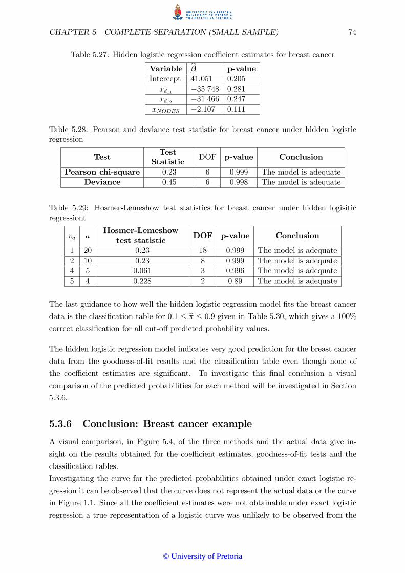
CHAPTER 5. COMPLETE SEPARATION (SMALL SAMPLE) 74
Table 5.27: Hidden logistic regression coe¢ cient estimates for breast cancer
Variable b� p-valueIntercept 41:051 0:205xd11 �35:748 0:281xd12 �31:466 0:247
xNODES �2:107 0:111
Table 5.28: Pearson and deviance test statistic for breast cancer under hidden logisticregression
TestTest
Statistic DOF p-value Conclusion
Pearson chi-square 0:23 6 0:999 The model is adequateDeviance 0:45 6 0:998 The model is adequate
Table 5.29: Hosmer-Lemeshow test statistics for breast cancer under hidden logisiticregressiont
va aHosmer-Lemeshow
test statistic DOF p-value Conclusion
1 20 0:23 18 0:999 The model is adequate2 10 0:23 8 0:999 The model is adequate4 5 0:061 3 0:996 The model is adequate5 4 0:228 2 0:89 The model is adequate
The last guidance to how well the hidden logistic regression model �ts the breast cancer
data is the classi�cation table for 0:1 � b� � 0:9 given in Table 5.30, which gives a 100%correct classi�cation for all cut-o¤ predicted probability values.
The hidden logistic regression model indicates very good prediction for the breast cancer
data from the goodness-of-�t results and the classi�cation table even though none of
the coe¢ cient estimates are signi�cant. To investigate this �nal conclusion a visual
comparison of the predicted probabilities for each method will be investigated in Section
5.3.6.
5.3.6 Conclusion: Breast cancer example
A visual comparison, in Figure 5.4, of the three methods and the actual data give in-
sight on the results obtained for the coe¢ cient estimates, goodness-of-�t tests and the
classi�cation tables.
Investigating the curve for the predicted probabilities obtained under exact logistic re-
gression it can be observed that the curve does not represent the actual data or the curve
in Figure 1.1. Since all the coe¢ cient estimates were not obtainable under exact logistic
regression a true representation of a logistic curve was unlikely to be observed from the
©© UUnniivveerrssiittyy ooff PPrreettoorriiaa

CHAPTER 5. COMPLETE SEPARATION (SMALL SAMPLE) 75
Table 5.30: Classi�cation table for breast cancer under hidden logistic regression forcut-o¤ probability from 0.1 to 0.9
Hidden logistic regressionb� Predictedvalues
Percentagecorrect
S D0:1 Observed S 10 0 100%to Values D 0 10 100%
0:9overall%
100%
Figure 5.4: Breast cancer example predicted probabilities for exact, Firth and hidden
observations
Pred
icte
dpr
obab
ilitie
s
20151050
1.0
0.8
0.6
0.4
0.2
0.0
0.5
Variable
FirthHLR
yExact
predicted probabilities. The predicted probabilities obtained under exact logistic regres-
sion reaches a maximum of b� = 0:5, this can explain why the classi�cation table predictedall the values to be yi = 0 for a predicted probability between 0:5 and 0:9:
Examining the predicted probabilities obtained under Firth�s model there is more of a
gradual increase from 0 to 1 than observed under the hidden logistic regression model.
The curve obtained from the predicted probabilities under Firth�s method resembles the
curve obtained in Figure 1.1, which serves as explanation for the signi�cant coe¢ cient
estimates, the results obtained from the goodness-of-�t tests and the perfect classi�cation
at b� = 0:5:Finally the hidden logistic regression model closely resembles the actual data same as for
the HIV example. This resemblance in the predicted probabilities obtained under the
hidden logistic regression model and the actual probabilities of the original data explains
the 100% correct classi�cation and the fact that the hidden logistic regression model is an
adequate model. This in turn also clari�es why the coe¢ cient estimates obtained under
the hidden logistic regression model are not signi�cant since there is still a horisontal
jump in the predicted probabilities from 0 to 1.
©© UUnniivveerrssiittyy ooff PPrreettoorriiaa
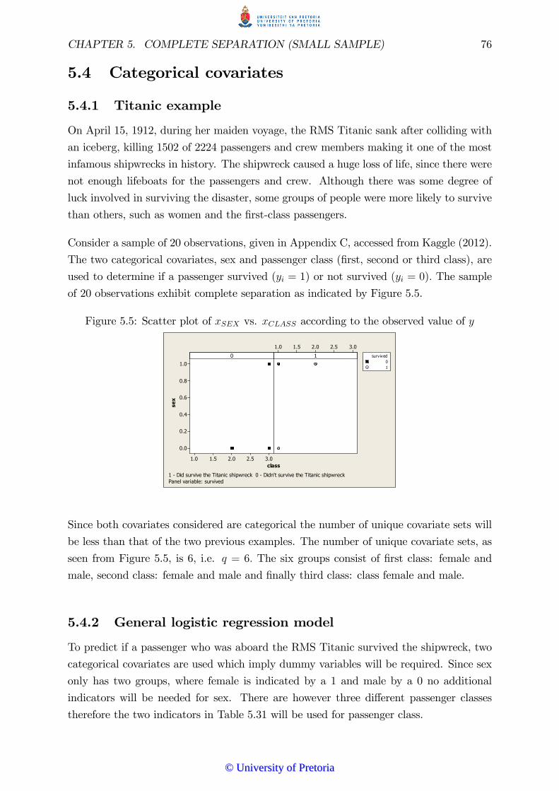
CHAPTER 5. COMPLETE SEPARATION (SMALL SAMPLE) 76
5.4 Categorical covariates
5.4.1 Titanic example
On April 15, 1912, during her maiden voyage, the RMS Titanic sank after colliding with
an iceberg, killing 1502 of 2224 passengers and crew members making it one of the most
infamous shipwrecks in history. The shipwreck caused a huge loss of life, since there were
not enough lifeboats for the passengers and crew. Although there was some degree of
luck involved in surviving the disaster, some groups of people were more likely to survive
than others, such as women and the �rst-class passengers.
Consider a sample of 20 observations, given in Appendix C, accessed from Kaggle (2012).
The two categorical covariates, sex and passenger class (�rst, second or third class), are
used to determine if a passenger survived (yi = 1) or not survived (yi = 0): The sample
of 20 observations exhibit complete separation as indicated by Figure 5.5.
Figure 5.5: Scatter plot of xSEX vs. xCLASS according to the observed value of y
class
sex
3.02.52.01.51.0
1.0
0.8
0.6
0.4
0.2
0.0
3.02.52.01.51.00 1 survived
01
Panel variable: survived1 Did survive the Titanic shipwreck 0 Didn't survive the Titanic shipwreck
Since both covariates considered are categorical the number of unique covariate sets will
be less than that of the two previous examples. The number of unique covariate sets, as
seen from Figure 5.5, is 6, i.e. q = 6: The six groups consist of �rst class: female and
male, second class: female and male and �nally third class: class female and male.
5.4.2 General logistic regression model
To predict if a passenger who was aboard the RMS Titanic survived the shipwreck, two
categorical covariates are used which imply dummy variables will be required. Since sex
only has two groups, where female is indicated by a 1 and male by a 0 no additional
indicators will be needed for sex. There are however three di¤erent passenger classes
therefore the two indicators in Table 5.31 will be used for passenger class.
©© UUnniivveerrssiittyy ooff PPrreettoorriiaa
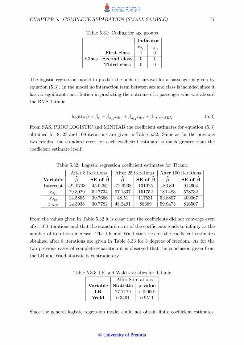
CHAPTER 5. COMPLETE SEPARATION (SMALL SAMPLE) 77
Table 5.31: Coding for age groups
Indicatorxd11 xd12
First class 1 0Class Second class 0 1
Third class 0 0
The logistic regression model to predict the odds of survival for a passenger is given by
equation (5.3). In the model no interaction term between sex and class is included since it
has no signi�cant contribution in predicting the outcome of a passenger who was aboard
the RMS Titanic.
logit(�i) = �0 + �d11xd11 + �d12xd12 + �SEXxSEX (5.3)
From SAS, PROC LOGISTIC and MINITAB the coe¢ cient estimates for equation (5.3)
obtained for 8, 25 and 100 iterations are given in Table 5.32. Same as for the previous
two results, the standard error for each coe¢ cient estimate is much greater than the
coe¢ cient estimate itself.
Table 5.32: Logistic regression coe¢ cient estimates for Titanic
After 8 iterations After 25 iterations After 100 iterationsVariable b� SE of b� b� SE of b� b� SE of b�Intercept -22.0708 45.0255 -72.9268 131925 -86.89 914604xd11 29.3929 52.7734 97.1337 151752 180.483 578732xd12 14.5855 39.7666 48.51 117531 53.8807 409067xSEX 14.3938 30.7782 48.2491 88369 59.9473 816507
From the values given in Table 5.32 it is clear that the coe¢ cients did not converge even
after 100 iterations and that the standard error of the coe¢ cients tends to in�nity as the
number of iterations increase. The LR and Wald statistics for the coe¢ cient estimates
obtained after 8 iterations are given in Table 5.33 for 3 degrees of freedom. As for the
two previous cases of complete separation it is observed that the conclusion given from
the LR and Wald statistic is contradictory.
Table 5.33: LR and Wald statistics for TitanicAfter 8 iterations
Variable Statistic p-valueLR 27:7129 < 0:0001Wald 0:3461 0:9511
Since the general logistic regression model could not obtain �nite coe¢ cient estimates,
©© UUnniivveerrssiittyy ooff PPrreettoorriiaa

CHAPTER 5. COMPLETE SEPARATION (SMALL SAMPLE) 78
the exact method, Firth�s method and hidden logistic regression will be applied to the
observations once again.
5.4.3 Exact logistic regression
Applying exact logistic regression to the data set given in Appendix C, the coe¢ cient
estimates given in Table 5.34 are obtained.
Table 5.34: Exact logistic regression coe¢ cient estimates for Titanic
Variable b� p-valueIntercept �3:1558 0:0054xd11 4:0444 0:0025xd12 1:4436 0:3333xSEX 2:1622 0:1333
As indicated from Table 5.34 all the coe¢ cients were obtainable since only categorical
covariates were considered for the exact method. Even though the indicator xd12 and
xSEX does not have signi�cant coe¢ cient estimates at a signi�cance level of � = 0:05,
the overall e¤ect of xd11 and xd12 is to be considered in the model.
By using the coe¢ cient estimates obtained in Table 5.34 in the logistic regression model
speci�ed by equation (5.3) the Pearson chi-square, deviance and Hosmer-Lemeshow test
statistics are given in Tables 5.35 and 5.36.
Table 5.35: Pearson and deviance test statistic for Titanic under exact logistic regression
TestTest
Statistic DOF p-value Conclusion
Pearson chi-square 4:0144 2 0:134 The model is adequateDeviance 0:1343 2 0:033 The model is not adequate
Table 5.36: Hosmer-Lemeshow test statistics for Titanic under exact logisitic regression
va aHosmer-Lemeshow
test statistic DOF p-value Conclusion
1 20 4:0144 18 0:999 The model is adequate2 10 4:0144 8 0:856 The model is adequate4 5 1:949 3 0:583 The model is adequate5 4 3:78 2 0:151 The model is adequate
The results obtained from Pearson�s chi-square and the deviance test statistic are con-
�icting. Pearson�s chi-square indicates that the model is adequate but on the other hand
©© UUnniivveerrssiittyy ooff PPrreettoorriiaa
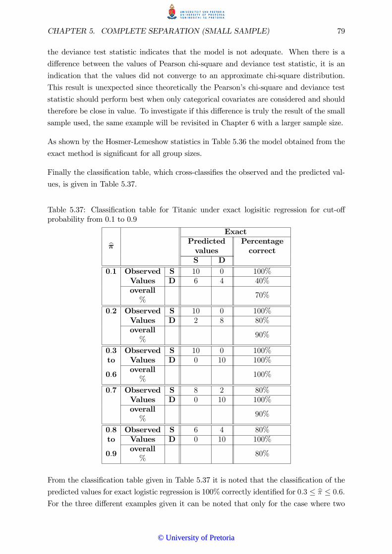
CHAPTER 5. COMPLETE SEPARATION (SMALL SAMPLE) 79
the deviance test statistic indicates that the model is not adequate. When there is a
di¤erence between the values of Pearson chi-square and deviance test statistic, it is an
indication that the values did not converge to an approximate chi-square distribution.
This result is unexpected since theoretically the Pearson�s chi-square and deviance test
statistic should perform best when only categorical covariates are considered and should
therefore be close in value. To investigate if this di¤erence is truly the result of the small
sample used, the same example will be revisited in Chapter 6 with a larger sample size.
As shown by the Hosmer-Lemeshow statistics in Table 5.36 the model obtained from the
exact method is signi�cant for all group sizes.
Finally the classi�cation table, which cross-classi�es the observed and the predicted val-
ues, is given in Table 5.37.
Table 5.37: Classi�cation table for Titanic under exact logisitic regression for cut-o¤probability from 0.1 to 0.9
Exactb� Predictedvalues
Percentagecorrect
S D0:1 Observed S 10 0 100%
Values D 6 4 40%overall%
70%
0:2 Observed S 10 0 100%Values D 2 8 80%overall%
90%
0:3 Observed S 10 0 100%to Values D 0 10 100%
0:6overall%
100%
0:7 Observed S 8 2 80%Values D 0 10 100%overall%
90%
0:8 Observed S 6 4 80%to Values D 0 10 100%
0:9overall%
80%
From the classi�cation table given in Table 5.37 it is noted that the classi�cation of the
predicted values for exact logistic regression is 100% correctly identi�ed for 0:3 � b� � 0:6:For the three di¤erent examples given it can be noted that only for the case where two
©© UUnniivveerrssiittyy ooff PPrreettoorriiaa
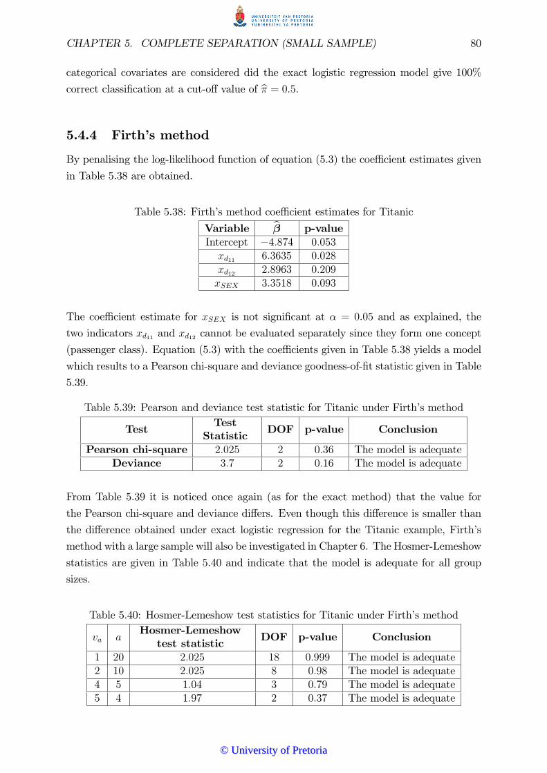
CHAPTER 5. COMPLETE SEPARATION (SMALL SAMPLE) 80
categorical covariates are considered did the exact logistic regression model give 100%
correct classi�cation at a cut-o¤ value of b� = 0:5:5.4.4 Firth�s method
By penalising the log-likelihood function of equation (5.3) the coe¢ cient estimates given
in Table 5.38 are obtained.
Table 5.38: Firth�s method coe¢ cient estimates for Titanic
Variable b� p-valueIntercept �4:874 0:053xd11 6:3635 0:028xd12 2:8963 0:209xSEX 3:3518 0:093
The coe¢ cient estimate for xSEX is not signi�cant at � = 0:05 and as explained, the
two indicators xd11 and xd12 cannot be evaluated separately since they form one concept
(passenger class). Equation (5.3) with the coe¢ cients given in Table 5.38 yields a model
which results to a Pearson chi-square and deviance goodness-of-�t statistic given in Table
5.39.
Table 5.39: Pearson and deviance test statistic for Titanic under Firth�s method
TestTest
Statistic DOF p-value Conclusion
Pearson chi-square 2:025 2 0:36 The model is adequateDeviance 3:7 2 0:16 The model is adequate
From Table 5.39 it is noticed once again (as for the exact method) that the value for
the Pearson chi-square and deviance di¤ers. Even though this di¤erence is smaller than
the di¤erence obtained under exact logistic regression for the Titanic example, Firth�s
method with a large sample will also be investigated in Chapter 6. The Hosmer-Lemeshow
statistics are given in Table 5.40 and indicate that the model is adequate for all group
sizes.
Table 5.40: Hosmer-Lemeshow test statistics for Titanic under Firth�s method
va aHosmer-Lemeshow
test statistic DOF p-value Conclusion
1 20 2:025 18 0:999 The model is adequate2 10 2:025 8 0:98 The model is adequate4 5 1:04 3 0:79 The model is adequate5 4 1:97 2 0:37 The model is adequate
©© UUnniivveerrssiittyy ooff PPrreettoorriiaa
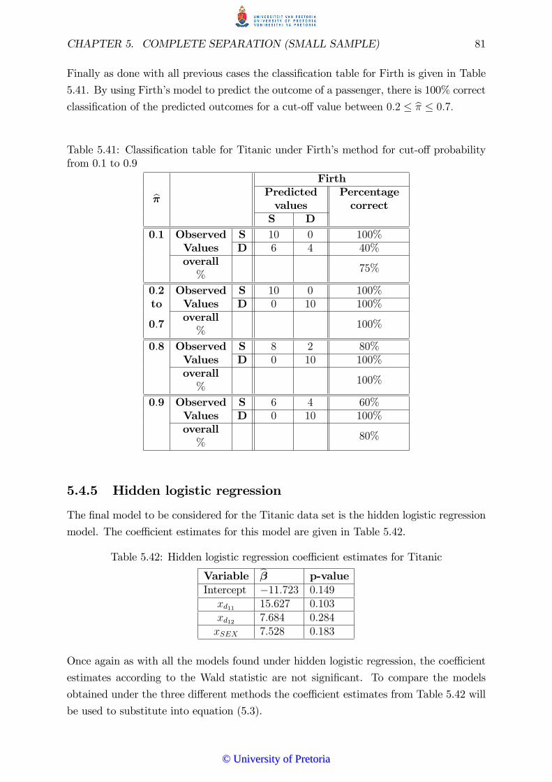
CHAPTER 5. COMPLETE SEPARATION (SMALL SAMPLE) 81
Finally as done with all previous cases the classi�cation table for Firth is given in Table
5.41. By using Firth�s model to predict the outcome of a passenger, there is 100% correct
classi�cation of the predicted outcomes for a cut-o¤ value between 0:2 � b� � 0:7:Table 5.41: Classi�cation table for Titanic under Firth�s method for cut-o¤ probabilityfrom 0.1 to 0.9
Firthb� Predictedvalues
Percentagecorrect
S D0:1 Observed S 10 0 100%
Values D 6 4 40%overall%
75%
0:2 Observed S 10 0 100%to Values D 0 10 100%
0:7overall%
100%
0:8 Observed S 8 2 80%Values D 0 10 100%overall%
100%
0:9 Observed S 6 4 60%Values D 0 10 100%overall%
80%
5.4.5 Hidden logistic regression
The �nal model to be considered for the Titanic data set is the hidden logistic regression
model. The coe¢ cient estimates for this model are given in Table 5.42.
Table 5.42: Hidden logistic regression coe¢ cient estimates for Titanic
Variable b� p-valueIntercept �11:723 0:149xd11 15:627 0:103xd12 7:684 0:284xSEX 7:528 0:183
Once again as with all the models found under hidden logistic regression, the coe¢ cient
estimates according to the Wald statistic are not signi�cant. To compare the models
obtained under the three di¤erent methods the coe¢ cient estimates from Table 5.42 will
be used to substitute into equation (5.3).
©© UUnniivveerrssiittyy ooff PPrreettoorriiaa

CHAPTER 5. COMPLETE SEPARATION (SMALL SAMPLE) 82
The goodness-of-�t statistics corresponding to the hidden logistic regression model are
given in Tables 5.43 and 5.44.
Table 5.43: Pearson and deviance test statistic for Titanic under hidden logistic regression
TestTest
Statistic DOF p-value Conclusion
Pearson chi-square 0:202 2 0:9 The model is adequateDeviance 0:399 2 0:819 The model is adequate
Table 5.44: Hosmer-Lemeshow test statistics for Titanic under hidden logisitic regression
va aHosmer-Lemeshow
test statistic DOF p-value Conclusion
1 20 0:202 18 0:999 The model is adequate2 10 0:202 8 0:999 The model is adequate4 5 0:106 3 0:991 The model is adequate5 4 0:201 2 0:9151 The model is adequate
As for all the previous hidden logistic regression models the coe¢ cient estimates are
not signi�cant but the model is adequate according to all goodness-of-�t tests. The
classi�cation table once again shows 100% correct classi�cation for all cut-o¤ values of b�,as seen in Table 5.45.
Table 5.45: Classi�cation table for Titanic under hidden logistic regression for cut-o¤probability from 0.1 to 0.9
Hidden logistic regressionb� Predictedvalues
Percentagecorrect
S D0:1 Observed S 10 0 100%to Values D 0 10 100%
0:9overall%
100%
5.4.6 Conclusion: Titanic example
When considering only categorical covariates the predicted probabilities of exact logistic
regression, Firth�s method and hidden logistic regression is represented in Figure 5.6.
As seen in Figure 5.6 the predicted probabilities of the exact logistic regression model
more closely resembles the logistic curve in Figure 1.1 and the actual data than obtained
©© UUnniivveerrssiittyy ooff PPrreettoorriiaa
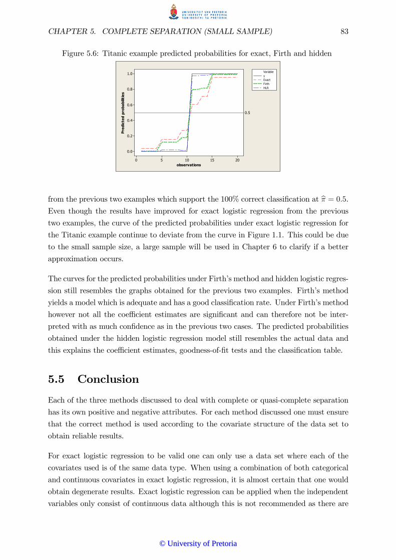
CHAPTER 5. COMPLETE SEPARATION (SMALL SAMPLE) 83
Figure 5.6: Titanic example predicted probabilities for exact, Firth and hidden
observations
Pred
icte
dpr
obab
ilitie
s
20151050
1.0
0.8
0.6
0.4
0.2
0.0
0.5
Variable
FirthHLR
yExact
from the previous two examples which support the 100% correct classi�cation at b� = 0:5.Even though the results have improved for exact logistic regression from the previous
two examples, the curve of the predicted probabilities under exact logistic regression for
the Titanic example continue to deviate from the curve in Figure 1.1. This could be due
to the small sample size, a large sample will be used in Chapter 6 to clarify if a better
approximation occurs.
The curves for the predicted probabilities under Firth�s method and hidden logistic regres-
sion still resembles the graphs obtained for the previous two examples. Firth�s method
yields a model which is adequate and has a good classi�cation rate. Under Firth�s method
however not all the coe¢ cient estimates are signi�cant and can therefore not be inter-
preted with as much con�dence as in the previous two cases. The predicted probabilities
obtained under the hidden logistic regression model still resembles the actual data and
this explains the coe¢ cient estimates, goodness-of-�t tests and the classi�cation table.
5.5 Conclusion
Each of the three methods discussed to deal with complete or quasi-complete separation
has its own positive and negative attributes. For each method discussed one must ensure
that the correct method is used according to the covariate structure of the data set to
obtain reliable results.
For exact logistic regression to be valid one can only use a data set where each of the
covariates used is of the same data type. When using a combination of both categorical
and continuous covariates in exact logistic regression, it is almost certain that one would
obtain degenerate results. Exact logistic regression can be applied when the independent
variables only consist of continuous data although this is not recommended as there are
©© UUnniivveerrssiittyy ooff PPrreettoorriiaa

CHAPTER 5. COMPLETE SEPARATION (SMALL SAMPLE) 84
models which give better results. Exact logistic regression performs the best when only
categorical covariates are used to predict the dependent variable.
When considering Firth�s method all covariate types, including a combination of categor-
ical and continuous, can be used. For all three cases of di¤erent covariates, most of the
coe¢ cient estimates obtained were signi�cant. By considering the overall goodness-of-�t
of Firth�s model, it was given as an adequate model according to Pearson�s chi-square, de-
viance and Hosmer-Lemeshow�s test statistic. For the classi�cation tables, 100% correct
classi�cation is obtained for a prede�ned estimated probability of 0.5.
Finally the hidden logistic regression model performed very well according to the classi�-
cation tables and to Pearson�s chi-square, deviance and Hosmer-Lemeshow�s test statistic.
A drawback of hidden logistic regression is the fact that it does not give signi�cant coef-
�cient estimates and that there is no prede�ned function in SAS (or any of the computer
programs mentioned in Chapter 2) available to calculate the coe¢ cient estimates. The
coe¢ cient estimates which are not signi�cant could be due to the small sample size and
will be investigated in Chapter 6 with a larger sample size.
Since all the examples considered in Chapter 5 are based on a small sample, the results
for Pearson�s chi-square and deviance test statistic should be interpreted with caution as
an approximate chi-square distribution might not have been obtained.
When considering the Hosmer-Lemeshow�s statistic other than the result depending on
the group sizes, it also depends on how many groups are chosen. If a few number of
groups are chosen then according to Xie (2008) it will almost always indicate that the
model �ts the data well. This can also be con�rmed for all examples where there is
only a few number of groups. For all cases where va is 1 or 2 the model is shown to be
an adequate model except for the exact logistic regression model applied to the breast
cancer data. Therefore when interpreting Hosmer-Lemeshow�s statistic one should rather
consider number of groups of four and higher.
When interpreting any of the models one should keep the statement of Box (1987) in
mind "All models are wrong, some models are useful". Therefore if the object of the
study is to resemble the true model as close as possible the hidden logistic regression
model will be suitable, if the object of the model is to eliminate most of the separation
present to the data set Firth�s model will work well. Each method is useful in its own
way and the model chosen depends on the desired outcome of the researcher.
©© UUnniivveerrssiittyy ooff PPrreettoorriiaa

Chapter 6
Quasi-complete separation (largesample)
6.1 Introduction
When coe¢ cient estimates of a logistic regression model are unobtainable due to non-
convergence for a practical application, the chances that quasi-complete separation is
present is much more likely than complete separation. This is especially true when
the sample size is large and continuous covariates or a combination of continuous and
categorical covariates are used. Since complete separation is a more severe case than
quasi-complete separation, all the approaches to deal with complete separation that have
been discussed can be used to deal with quasi-complete separation. To demonstrate
non-convergence of coe¢ cient estimates for a large sample, the Titanic example of Kag-
gle (2012) will be revisited. When the sample size is increased to 100, quasi-complete
separation is observed in the data set.
6.2 Categorical covariates
6.2.1 Titanic example: large sample
By considering the Titanic example in Appendix D as discussed in Section 5.4.1 from
Kaggle (2012) the logistic regression model stays the same as given in equation (5.3)
with indicators discussed in Table 5.31. For 100 randomly selected cases, quasi-complete
separation is present in the data set, which means that each covariate set is not unique
to either yi = 1 (survived) or yi = 0 (did not survive) since some covariate sets present
both yi = 1 and yi = 0, as represented in Figure 6.1.
85
©© UUnniivveerrssiittyy ooff PPrreettoorriiaa

CHAPTER 6. QUASI-COMPLETE SEPARATION (LARGE SAMPLE) 86
Figure 6.1: Large sample scatter plot of xSEX vs. xCLASS according to the observed valueof y
class
sex
3.02.52.01.51.0
1.0
0.8
0.6
0.4
0.2
0.0
survived01
1 Did Survive the Titanic shipwreck 0 Didn't survive the Titanic shipwreck
6.2.2 General logistic regression model revisited
From SAS, PROC LOGISTIC the coe¢ cient estimates for the logistic regression model
in equation (5.3) is represented in Table 6.1 for 8, 25 and 100 iterations respectively.
From Table 6.1 one can note that the coe¢ cient estimates still did not converge after
100 iterations, but the standard errors for the coe¢ cients are smaller than for the case
of complete separation. The coe¢ cient estimates and the standard error are also very
similar for all coe¢ cient estimates whereas for complete separation the standard error
di¤ered by a noticeable amount for the di¤erent coe¢ cient estimates. The standard
error for the coe¢ cient estimates are still larger than the coe¢ cient estimate itself for all
coe¢ cient estimates.
Table 6.1: Logistic regression coe¢ cient estimates for Titanic: large sample
After 8 iterations After 25 iterations After 100 iterationsVariable b� SE of b� b� SE of b� b� SE of b�Intercept �11:2245 12:977 �28:2247 38599 �103:32 162225xd11 8:7396 12:9884 25:7398 38599 100:83 162225xd12 8:6596 12:9685 25:6598 38599 100:75 162225xSEX 11:3299 12:9695 28:3301 38599 103:42 162225
Nevertheless, even if the standard errors are smaller than for complete separation, the
coe¢ cient estimates still do not converge after 100 iterations. To investigate signi�cance
of the coe¢ cient estimates obtained after 8 iterations the Wald and LR statistic are
studied in Table 6.2. From this it can be noted both tests reject the null hypothesis,
which implies that both tests indicate that the coe¢ cient estimates used in the model are
signi�cant. This conclusion is obtained for 8 iterations and is con�icting with the fact
that the coe¢ cient estimates did not converge. From this it can be observed that for a
©© UUnniivveerrssiittyy ooff PPrreettoorriiaa
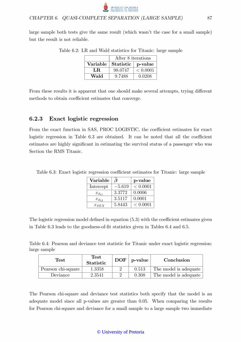
CHAPTER 6. QUASI-COMPLETE SEPARATION (LARGE SAMPLE) 87
large sample both tests give the same result (which wasn�t the case for a small sample)
but the result is not reliable.
Table 6.2: LR and Wald statistics for Titanic: large sample
After 8 iterationsVariable Statistic p-valueLR 98:0747 < 0:0001Wald 9:7488 0:0208
From these results it is apparent that one should make several attempts, trying di¤erent
methods to obtain coe¢ cient estimates that converge.
6.2.3 Exact logistic regression
From the exact function in SAS, PROC LOGISTIC, the coe¢ cient estimates for exact
logistic regression in Table 6.3 are obtained. It can be noted that all the coe¢ cient
estimates are highly signi�cant in estimating the survival status of a passenger who was
Section the RMS Titanic.
Table 6.3: Exact logistic regression coe¢ cient estimates for Titanic: large sample
Variable b� p-valueIntercept �5:619 < 0:0001xd11 3:3772 0:0006xd12 3:5117 0:0001xSEX 5:8443 < 0:0001
The logistic regression model de�ned in equation (5.3) with the coe¢ cient estimates given
in Table 6.3 leads to the goodness-of-�t statistics given in Tables 6.4 and 6.5.
Table 6.4: Pearson and deviance test statistic for Titanic under exact logistic regression:large sample
TestTest
Statistic DOF p-value Conclusion
Pearson chi-square 1:3358 2 0:513 The model is adequateDeviance 2:3541 2 0:308 The model is adequate
The Pearson chi-square and deviance test statistics both specify that the model is an
adequate model since all p-values are greater than 0.05. When comparing the results
for Pearson chi-square and deviance for a small sample to a large sample two immediate
©© UUnniivveerrssiittyy ooff PPrreettoorriiaa
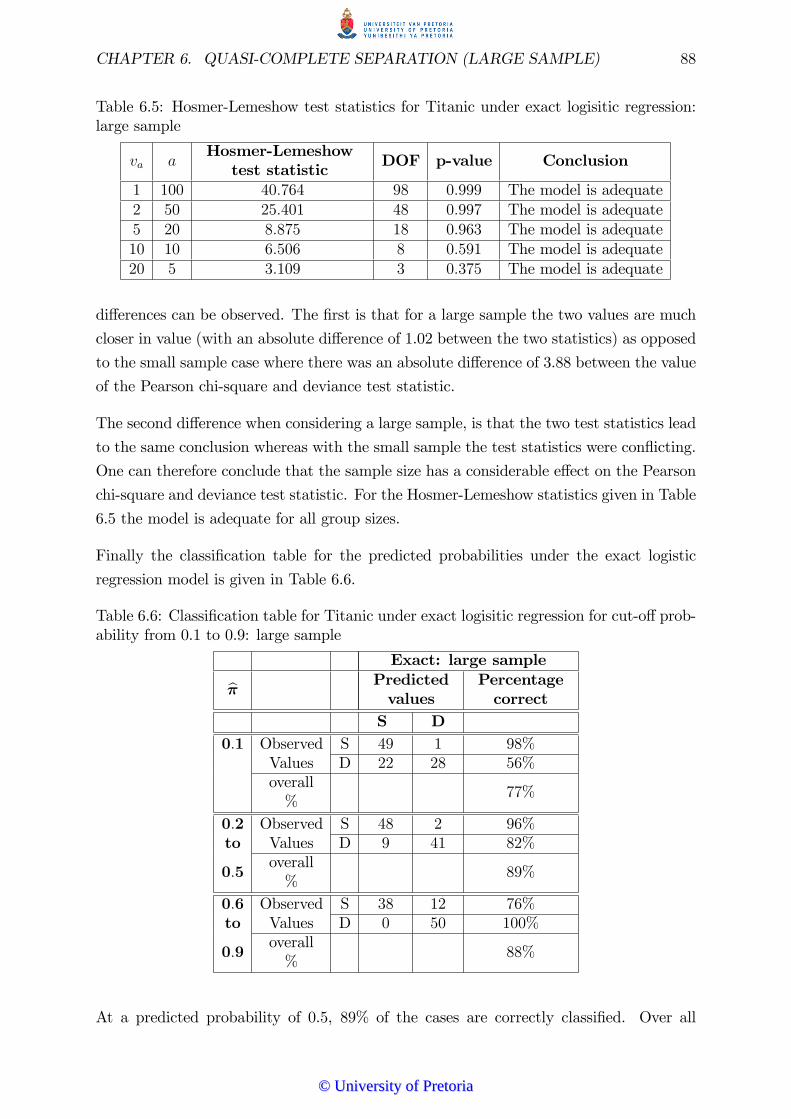
CHAPTER 6. QUASI-COMPLETE SEPARATION (LARGE SAMPLE) 88
Table 6.5: Hosmer-Lemeshow test statistics for Titanic under exact logisitic regression:large sample
va aHosmer-Lemeshow
test statistic DOF p-value Conclusion
1 100 40:764 98 0:999 The model is adequate2 50 25:401 48 0:997 The model is adequate5 20 8:875 18 0:963 The model is adequate10 10 6:506 8 0:591 The model is adequate20 5 3:109 3 0:375 The model is adequate
di¤erences can be observed. The �rst is that for a large sample the two values are much
closer in value (with an absolute di¤erence of 1.02 between the two statistics) as opposed
to the small sample case where there was an absolute di¤erence of 3.88 between the value
of the Pearson chi-square and deviance test statistic.
The second di¤erence when considering a large sample, is that the two test statistics lead
to the same conclusion whereas with the small sample the test statistics were con�icting.
One can therefore conclude that the sample size has a considerable e¤ect on the Pearson
chi-square and deviance test statistic. For the Hosmer-Lemeshow statistics given in Table
6.5 the model is adequate for all group sizes.
Finally the classi�cation table for the predicted probabilities under the exact logistic
regression model is given in Table 6.6.
Table 6.6: Classi�cation table for Titanic under exact logisitic regression for cut-o¤ prob-ability from 0.1 to 0.9: large sample
Exact: large sampleb� Predictedvalues
Percentagecorrect
S D0:1 Observed S 49 1 98%
Values D 22 28 56%overall%
77%
0:2 Observed S 48 2 96%to Values D 9 41 82%
0:5overall%
89%
0:6 Observed S 38 12 76%to Values D 0 50 100%
0:9overall%
88%
At a predicted probability of 0.5, 89% of the cases are correctly classi�ed. Over all
©© UUnniivveerrssiittyy ooff PPrreettoorriiaa
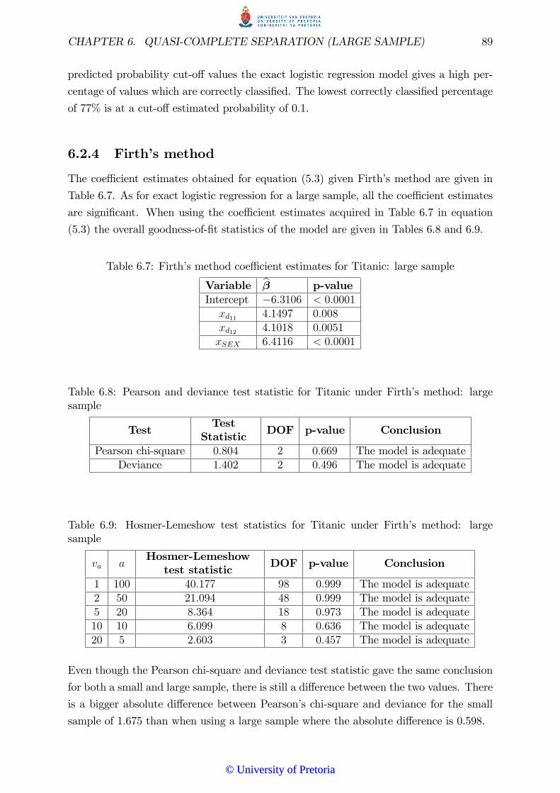
CHAPTER 6. QUASI-COMPLETE SEPARATION (LARGE SAMPLE) 89
predicted probability cut-o¤ values the exact logistic regression model gives a high per-
centage of values which are correctly classi�ed. The lowest correctly classi�ed percentage
of 77% is at a cut-o¤ estimated probability of 0.1.
6.2.4 Firth�s method
The coe¢ cient estimates obtained for equation (5.3) given Firth�s method are given in
Table 6.7. As for exact logistic regression for a large sample, all the coe¢ cient estimates
are signi�cant. When using the coe¢ cient estimates acquired in Table 6.7 in equation
(5.3) the overall goodness-of-�t statistics of the model are given in Tables 6.8 and 6.9.
Table 6.7: Firth�s method coe¢ cient estimates for Titanic: large sample
Variable b� p-valueIntercept �6:3106 < 0:0001xd11 4:1497 0:008xd12 4:1018 0:0051xSEX 6:4116 < 0:0001
Table 6.8: Pearson and deviance test statistic for Titanic under Firth�s method: largesample
TestTest
Statistic DOF p-value Conclusion
Pearson chi-square 0:804 2 0:669 The model is adequateDeviance 1:402 2 0:496 The model is adequate
Table 6.9: Hosmer-Lemeshow test statistics for Titanic under Firth�s method: largesample
va aHosmer-Lemeshow
test statistic DOF p-value Conclusion
1 100 40:177 98 0:999 The model is adequate2 50 21:094 48 0:999 The model is adequate5 20 8:364 18 0:973 The model is adequate10 10 6:099 8 0:636 The model is adequate20 5 2:603 3 0:457 The model is adequate
Even though the Pearson chi-square and deviance test statistic gave the same conclusion
for both a small and large sample, there is still a di¤erence between the two values. There
is a bigger absolute di¤erence between Pearson�s chi-square and deviance for the small
sample of 1.675 than when using a large sample where the absolute di¤erence is 0.598.
©© UUnniivveerrssiittyy ooff PPrreettoorriiaa

CHAPTER 6. QUASI-COMPLETE SEPARATION (LARGE SAMPLE) 90
Given the goodness-of-�t tests, including the Hosmer-Lemeshow test statistics for any
number of groups, the overall �t of Firth�s model is adequate.
Table 6.10: Classi�cation table for Titanic under Firth�s method for cut-o¤ probabilityfrom 0.1 to 0.9: large sample
Firth: large sampleb� Predictedvalues
Percentagecorrect
S D0:1 Observed S 49 1 98%
Values D 21 29 58%overall%
78%
0:2 Observed S 48 2 96%to Values D 9 41 82%
0:5overall%
89%
0:6 Observed S 38 12 76%to Values D 0 50 100%
0:9overall%
88%
Once again when considering the classi�cation table given in Table 6.10 one can note
that at a predicted probability of 0.5, the number of correctly classi�ed observations is
89 out of a total of 100, identical to the classi�cation of exact logistic regression.
6.2.5 Hidden logistic regression
The �nal model to be considered for the large sample case of predicting the survival
status of a passenger who was Section the RMS Titanic is the hidden logistic regression
model. The coe¢ cient estimates given in Table 6.11 are all signi�cant according to the
Wald test statistic, in accordance with the rest of the models using a large sample. This
is the �rst example considered where the coe¢ cient estimates obtained under the hidden
logistic regression model are all signi�cant.
The overall goodness-of-�t of the model is evaluated by interpreting the Pearson chi-
square, deviance and Hosmer-Lemeshow test statistics. The absolute di¤erence between
Pearson chi-square and deviance test statistic as seen from Table 6.12 is 0.268. The
di¤erence between these two values is the smallest for all the methods mentioned using
a large sample.
©© UUnniivveerrssiittyy ooff PPrreettoorriiaa

CHAPTER 6. QUASI-COMPLETE SEPARATION (LARGE SAMPLE) 91
Table 6.11: Hidden logistic regression coe¢ cient estimates for Titanic: large sample
Variable b� p-valueIntercept �7:309 0:0005xd11 4:906 0:0225xd12 4:851 0:0181xSEX 7:428 0:0003
Table 6.12: Pearson and deviance test statistic for Titanic under hidden logistic regres-sion: large sample
TestTest
Statistic DOF p-value Conclusion
Pearson chi-square 0:287 2 0:866 The model is adequateDeviance 0:554 2 0:758 The model is adequate
The Hosmer-Lemeshow test statistics values in Table 6.13 also con�rm that the hidden
logistic regression model for a large sample is adequate.
Table 6.13: Hosmer-Lemeshow test statistics for Titanic under hidden logisitic regression:large sample
va aHosmer-Lemeshow
test statistic DOF p-value Conclusion
1 100 44:220 98 0:999 The model is adequate2 50 21:493 48 0:999 The model is adequate5 20 7:963 18 0:979 The model is adequate10 10 5:377 8 0:717 The model is adequate20 5 1:859 3 0:602 The model is adequate
Finally the classi�cation table in Table 6.14 revealed that the hidden logistic regression
model could correctly classify 89% of the observations at b� = 0:5 which is the same asfor exact logistic regression and Firth�s method for the large sample case.
6.3 Conclusion
As examined for all the small sample cases, a visual representation of the predicted
probabilities for exact logistic regression, Firth�s method and hidden logistic regression
are shown in Figure 6.2.
The �rst noticeable di¤erence between the small sample case and the large sample case,
is that for the large sample case the curve for the predicted probabilities for all three
methods are almost exactly similar. From Figure 6.2 one can explain the 89% correctly
classi�ed values given for all methods and the similar results obtained from the goodness-
of-�t tests. For the large sample case the di¤erence between the coe¢ cient estimates for
©© UUnniivveerrssiittyy ooff PPrreettoorriiaa

CHAPTER 6. QUASI-COMPLETE SEPARATION (LARGE SAMPLE) 92
Table 6.14: Classi�cation table for Titanic under hidden logisitic regression for cut-o¤probability from 0.1 to 0.9: large sample
Hidden: large sampleb� Predictedvalues
Percentagecorrect
S D0:1 Observed S 48 2 96%to Values D 9 41 82%
0:5overall%
77%
0:6 Observed S 38 12 76%to Values D 0 50 100%
0:9overall%
88%
Figure 6.2: Large sample Titanic example predicted probabilities for exact, Firth andhidden
observations
Pred
icte
dpr
obab
ilitie
s
100806040200
1.0
0.8
0.6
0.4
0.2
0.0
0.5
Variable
FirthHLR
yExact
all three methods are much smaller than for the small sample case. From this one can
conclude that for the case where only categorical covariates are used, as the sample size
increases, the coe¢ cient estimates obtained for exact logistic regression, Firth�s method
and hidden logistic regression approximates to the same value.
When considering the Titanic example other di¤erences between the small and the large
sample case were observed.
The �rst noticeable di¤erence is the fact that the Wald, Pearson chi-square and deviance
test statistics gave more reliable results, due to the fact that with a large sample one can
be more certain of the fact that an approximate chi-square distribution is obtained.
The second noticeable di¤erence is that the percentage of correctly classi�ed observations
has decreased to 89% for all methods at a cut-o¤ predicted probability of 0.5 where it
©© UUnniivveerrssiittyy ooff PPrreettoorriiaa

CHAPTER 6. QUASI-COMPLETE SEPARATION (LARGE SAMPLE) 93
was 100% for all methods for the small sample case. Even though this is the case, for
the large sample all the coe¢ cient estimates obtained under all methods are signi�cant
which enables one to interpret the results with more con�dence than for the small sample
case.
When considering the di¤erent methods, exact logistic regression and Firth�s method in-
creased in performance from the Pearson chi-square, deviance and Hosmer-Lemeshow test
statistics are considered. All of the corresponding p-values for the above mentioned tests
increased for both exact logistic regression and for Firth�s method. From the goodness-
of-�t measures for the two above-mentioned methods, one also notices that the di¤erence
between Pearson�s chi-square and the deviance test statistic became smaller for the large
sample case than it was for the small sample. Given all these improvements for the large
sample case it must also be mentioned that complete or quasi-complete separation is
much more unlikely in a large sample than it is in a small sample.
©© UUnniivveerrssiittyy ooff PPrreettoorriiaa
Chapter 7
Summary and Conclusion
A logistic regression model predicts the outcome of a dichotomous variable based on a set
of covariates. When deriving a logistic regression model it is very important to investigate
the type of covariates present in your data set. When interpreting goodness of �t tests
it is important to bear in mind that Pearson�s chi-square and the deviance test statistic
perform best when the sample size is large and when categorical covariates are considered.
Hosmer-Lemeshow�s statistic is in�uenced by the group sizes and the number of groups
chosen
When constructing a logistic regression model the coe¢ cient estimates do not always
exist. Therefore it is essential to test whether complete or quasi-complete separation is
present in a data set when the dependent variable is dichotomous, especially when the
sample size is small. When complete or quasi-complete separation is present in the data
set it is imperative not to continue with the general approach of a logistic regression
model, but to follow a di¤erent tactic.
Many di¤erent solutions for complete and quasi-complete separation exist in practice.
Each method has its own bene�ts and disadvantages and these should be investigated
before applying the method to your data set. For the methods which were investigated,
exact logistic regression performs well with categorical covariates but caution should be
applied when using this method to a sparse data set. Firth�s method gives signi�cant
coe¢ cient estimates for most cases and transforms the data to represent a logistic curve
which gradually increases to an estimated probability from 0 to 1. Finally the hidden
logistic regression model gives perfect classi�cation for all cases, but still closely resembles
a model under complete or quasi complete separation.
For exact logistic regression one can only use a data set where each of the covariates used
are of the same data type. When using a combination of both categorical and continuous
covariates in exact logistic regression, it is almost certain that one would obtain unreliable
results. Exact logistic regression can be used when the independent variables only consist
94
©© UUnniivveerrssiittyy ooff PPrreettoorriiaa

CHAPTER 7. SUMMARY AND CONCLUSION 95
of continuous data although this is not recommended. Exact logistic regression performs
the best when only categorical covariates are used to predict the dependent variable.
When considering Firth�s method or hidden logistic regression all covariate types, includ-
ing a combination of categorical and continuous, can be used. The coe¢ cient estimates
for exact logistic regression and Firth�s method can be obtained with available functions
in SAS. A drawback of hidden logistic regression is that there is no prede�ned function
in SAS (or any of the computer programs mentioned in Chapter 2) available to calculate
the coe¢ cient estimates.
For the large sample case there was a remarkable improvement in exact logistic regression,
Firth�s method and hidden logistic regression compared to a small sample.
Future work could comprise of including more covariates in the model and analysing
the model �t statistics to compare the e¤ect of including and excluding covariates in
the di¤erent models; multicollinearity in the models can be explored, and the presence
of outliers evaluated. The di¤erent methods to deal with complete or quasi-complete
separation mentioned in Section 3.2, not covered in this dissertation, can be investigated
for di¤erent covariate types and sample sizes.
The scope which have been covered in this dissertation expresses the importance in reval-
uating the model when either complete or quasi-complete separation is obtained in the
data. It also highlights the di¤erences among the three methods investigated (exact lo-
gistic regression, Firth�s method and hidden logistic regression) and the fact that each
method cannot be used in any scenario. Finally it was shown how the goodness of �t
methods can di¤er based on the type of covariates used, sample size and group sizes.
©© UUnniivveerrssiittyy ooff PPrreettoorriiaa

References
ABRAHANTES, J. C. and AERTS, M. (2012). A solution to separation for clustered
binary data. Statistical Modelling 12, 3-27.
AGRESTI, A. (1990). Categorical data analysis. Wiley.
AGRESTI, A. (1996). An Introduction to Categorical Data Analysis. Wiley.
ALBERT, A. and ANDERSON, J. (1984). On the existence of maximum likelihood
estimates in logistic regression models. Biometrika 71, 1-10.
ALLISON, P., ALTMAN, M., GILL, J. and MCDONALD, M. P. (2004). Convergence
problems in logistic regression. Numerical issues in statistical computing for the
social scientist, 238-252.
ALLISON, P. D. (2012). Logistic regression using SAS: Theory and application. SAS
Institute.
BEGGS, S., CARDELL, S. and HAUSMAN, J. (1981). Assessing the potential demand
for electric cars. Journal of econometrics 17, 1-19.
BERTOLINI, G., DAMICO, R., NARDI, D., TINAZZI, A. and APOLONE, G. (2000).
One model, several results: the paradox of the Hosmer-Lemeshow goodness-of-�t
test for the logistic regression model. Journal of epidemiology and biostatistics 5,
251-253.
BOX, G. E. P. and DRAPER, N. R. (1987). Empirical model-building and response
surfaces. Wiley.
CHAPMAN, R. G. (1984). An Approach to Estimating Logit Models of a Single Decision
Maker�s Choice Behavior. Advances in Consumer Research 11, 656-661.
CHRISTMANN, A. and ROUSSEEUW, P. J. (2001). Measuring overlap in binary
regression. Computational Statistics and Data Analysis 37, 65-75.
96
©© UUnniivveerrssiittyy ooff PPrreettoorriiaa

REFERENCES 97
CLOGG, C. C., RUBIN, D. B., SCHENKER, N., SCHULTZ, B. and WEIDMAN, L.
(1991). Multiple imputation of industry and occupation codes in census public-
use samples using Bayesian logistic regression. Journal of the American Statistical
Association 86, 68-78.
COLLETT, D. (2003). Modelling Binary Data. Chapman and Hall/CRC.
COPAS, J. (1988). Binary regression models for contaminated data. Journal of the
Royal Statistical Society. Series B (Methodological), 225-265.
COX, D. R. and HINKLEY, D. V. (1979). Theoretical Statistics. Chapman and Hall.
COX, D. R. and SNELL, E. J. (1989). Analysis of Binary Data. Chapman and Hall.
DAY, N. E. and KERRIDGE, D. F. (1967). A general maximum likelihood discriminant.
Biometrics, 313-323.
DYKE, G. and PATTERSON, H. (1952). Analysis of factorial arrangements when the
data are proportions. Biometrics 8, 1-12.
EKHOLM, A. and PALMGREN, J. (1982). A model for a binary response with misclas-
si�cations. Proceedings of the GLIM 82: Proceedings of the international conference
on generalised linear models, 128-143.
FIRTH, D. (1992a). Bias reduction, the Je¤erys prior and GLIM. Advances in GLIM
and statistical modelling: proceedings of the GLIM92 Conference and the 7th In-
ternational Workshop on Statistical Modelling, Munich, 13-17 July 1992: Springer-
Verlag.
FIRTH, D. (1992b). Generalized linear models and je¤reys priors: an iterative weighted
l east-squares approach. Computational statistics 1, 553-557.
FIRTH, D. (1993). Bias reduction of maximum likelihood estimates. Biometrika 80,
27-38.
GAO, S. and SHEN, J. (2007). Asymptotic properties of a double penalised maximum
likelihood estimator in logistic regression. Statistics and probability letters 77, 925-
930.
HABERMAN, S. (1973). Generalized Residuals for Log-Linear Models. Proceedings of
the 9th International Biometrics Conference. Boston, pp. p. 104-122.
HEINZE, G. (2006). A comparative investigation of methods for logistic regression with
separated or nearly separated data. Statistics in medicine 25, 4216-4226.
©© UUnniivveerrssiittyy ooff PPrreettoorriiaa

REFERENCES 98
HEINZE, G. and SCHEMPER, M. (2002). A solution to the problem of separation in
logistic regression. Statistics in medicine 21, 2409-2419.
HOSMER, D. W., LEMESHOW, S. and COOK, E. D. (2001). Applied Logistic Regres-
sion, Second Edition: Book and Solutions Manual Set. Wiley.
JEFFREYS, H. (1946). An invariant form for the prior probability in estimation prob-
lems. Proceedings of the Royal Society of London. Series A. Mathematical and
Physical Sciences 186, 453-461.
KAGGLE (2012).Go from Big Data to Big Analytics. [ONLINE] Available at:
https://www.kaggle.com/c/titanic-gettingStarted/data. [Accessed 01 June 13]
KING, E. N. and RYAN, T. P. (2002). A preliminary investigation of maximum likeli-
hood logistic regression versus exact logistic regression. The American Statistician
56, 163-170.
LIU, Y. (2007). On Goodness-of-Fit of Logistic Regression Model. Department of
Statistics. Kansas: Kansas State University.
LLOYD, C. J. (1999). Statistical analysis of categorical data. Wiley.
MCCULLAGH, P. and NELDER, J. A. (1989). Generalized Linear Models. Chapman
and Hall.
MEHTA, C. R. and PATEL, N. R. (1995). Exact logistic regression: theory and exam-
ples. Statistics in medicine 14, 2143-2160.
PEARSON, K. (1900). X. On the criterion that a given system of deviations from the
probable in the case of a correlated system of variables is such that it can be rea-
sonably supposed to have arisen from random sampling. The London, Edinburgh,
and Dublin Philosophical Magazine and Journal of Science 50, 157-175.
PHILIPPEOS, C., STEFFENS, F. and MEYER, D. (2009). Comparative 1H NMR-
based metabonomic analysis of HIV-1 sera. Journal of biomolecular NMR 44, 127-
137.
QUENOUILLE, M. H. (1949). Approximate tests of correlation in time-series 3. Pro-
ceedings of the Mathematical Proceedings of the Cambridge Philosophical Society,
483-484.
QUENOUILLE, M. H. (1956). Notes on bias in estimation. Biometrika 43, 353-360.
RAO, C. R. (1973). Linear Statistical Inference and Its Applications. Wiley.
©© UUnniivveerrssiittyy ooff PPrreettoorriiaa

REFERENCES 99
ROUSSEEUW, P. J. and CHRISTMANN, A. (2003). Robustness against separation
and outliers in logistic regression. Computational Statistics and Data Analysis 43,
315-332.
SANTNER, T. J. and DUFFY, D. E. (1986). A note on A. Albert and JA Anderson�s
conditions for the existence of maximum likelihood estimates in logistic regression
models. Biometrika 73, 755-758.
SILVAPULLE, M. J. (1981). On the existence of maximum likelihood estimators for
the binomial response models. Journal of the Royal Statistical Society. Series B
(Methodological), 310-313.
XIE, X.-J., PENDERGAST, J. and CLARKE, W. (2008). Increasing the power: A prac-
tical approach to goodness-of-�t test for logistic regression models with continuous
predictors. Computational Statistics and Data Analysis 52, 2703-2713.
ZORN, C. (2005). A solution to separation in binary response models. Political Analysis
13, 157-170.
©© UUnniivveerrssiittyy ooff PPrreettoorriiaa

Appendix A: Data on HIV statuspatients
HIV Status V3.74 V1.181 �0:4 1:631 �0:42 1:621 �0:44 1:791 �0:45 1:81 �0:46 1:991 �0:35 1:441 �0:45 1:611 �0:38 1:61 �0:5 1:851 �0:45 1:610 �0:29 1:730 �0:48 2:360 �0:36 1:950 �0:02 1:260 �0:26 1:80 �0:28 1:740 �0:24 2:270 �0:26 1:490 �0:27 1:710 �0:27 1:54
100
©© UUnniivveerrssiittyy ooff PPrreettoorriiaa

Appendix B: Data on breast cancerpatients
Outcome + nodes age group1 2 21 3 21 0 11 2 21 0 11 0 11 0 11 2 21 3 21 2 20 22 30 12 20 7 20 11 20 7 20 6 20 7 20 19 20 6 20 20 2
101
©© UUnniivveerrssiittyy ooff PPrreettoorriiaa

Appendix C: Data on Titanicpassengers: small sample
Survived Class Sex1 1 11 2 11 1 11 1 11 1 11 1 11 2 11 1 11 1 01 1 00 3 00 2 00 3 00 2 00 3 00 2 00 2 00 3 10 3 00 3 1
102
©© UUnniivveerrssiittyy ooff PPrreettoorriiaa

Appendix D: Data on Titanicpassengers: large sample
S Class Sex S Class Sex S Class Sex S Class Sex S Class Sex1 1 1 1 2 1 1 3 1 0 1 0 0 2 01 1 1 1 2 1 1 3 1 0 1 0 0 2 01 1 1 1 2 1 1 3 1 0 1 0 0 2 01 1 1 1 2 1 1 3 1 0 1 0 0 2 01 1 1 1 2 1 1 3 1 0 1 0 0 3 01 1 1 1 2 1 1 3 1 0 1 0 0 3 01 1 1 1 2 1 1 3 1 0 1 0 0 3 01 1 1 1 2 1 1 3 1 0 1 0 0 3 01 1 1 1 2 1 1 1 0 0 1 0 0 3 01 1 1 1 2 1 1 2 0 0 1 0 0 3 01 1 1 1 2 1 0 3 1 0 1 0 0 3 01 1 1 1 2 1 0 3 1 0 2 0 0 3 01 1 1 1 2 1 0 3 1 0 2 0 0 3 01 1 1 1 2 1 0 3 1 0 2 0 0 3 01 1 1 1 2 1 0 3 1 0 2 0 0 3 01 2 1 1 2 1 0 3 1 0 2 0 0 3 01 2 1 1 2 1 0 3 1 0 2 0 0 3 01 2 1 1 2 1 0 3 1 0 2 0 0 3 01 2 1 1 3 1 0 3 1 0 2 0 0 3 01 2 1 1 3 1 0 1 0 0 2 0 0 3 0
103
©© UUnniivveerrssiittyy ooff PPrreettoorriiaa

Appendix E: SAS program code forpenalised likelihood function
proc iml;
y={input values};
x1={input values};
n=nrow(y);
x0=J(n,1,1);
intercept=x0*b0;
X=x0||x1;
values=J(20,3,0);
logl=J(n,1,0);
W=J(n,n,0);
do beta=0.1 to 2 by 0.1;
x1beta=x1*beta;
fullx=intercept||x1beta;
do i=1 to n;
xirow=fullx[i,+];
W[i,i]=((exp(xirow))/(1+exp(xirow)))*(1/(1+exp(xirow)));
logl[i,1]=y[i,1]*xirow-log(1+exp(xirow));
total=logl[+];
end;
Xtrans=X�;
Fisher=Xtrans*W*X;
detF=det(Fisher);
print fisher detF;
plogl=total+(0.5)*log(detF);
ind=beta*10;
104
©© UUnniivveerrssiittyy ooff PPrreettoorriiaa
APPENDIX E: SAS PROGRAMCODEFORPENALISED LIKELIHOODFUNCTION105
values[ind,1]=beta;
values[ind,2]=total;
values[ind,3]=plogl;
end;
print values;
cn = {�beta� �LogL� �PenLogL�};
create outputval from values[colname=cn];
append from values;
run;
goptions reset=all i=join;
proc gplot data=outputval;
plot PenLogL*beta;
run;
quit;
©© UUnniivveerrssiittyy ooff PPrreettoorriiaa

Appendix F: SAS program code forclassi�cation tables
proc iml;
Beta={input values};
y={input values};
x={inut values as matrix};
n=nrow(y);
intercept=J(n,1,1);
fullx=intercept||x;
print firthbeta y x fullx;
logodds=fullx*firthbeta;
results=J(10,5,0);
do prob=0.1 to 0.9 by 0.1;
ind=prob*10;
count=J(n,1,0);
cc=0;
Obs1pred0=0;
obs0pred1=0;
obs1pred1=0;
obs0pred0=0;
logoddsCO=log(prob/(1-prob));
testlogodds=J(n,1,logoddsCO);
diff=logodds-testlogodds;
do i=1 to n;
if diff[i,1]>0 then count[i,1]=1;
groups=y-count;
if groups[i,1]=0 then cc=cc+1;
if groups[i,1]=1 then obs1pred0=obs1pred0+1;
106
©© UUnniivveerrssiittyy ooff PPrreettoorriiaa
APPENDIX F: SAS PROGRAM CODE FOR CLASSIFICATION TABLES 107
if groups[i,1]=-1 then obs0pred1=obs0pred1+1;
end;
do j=1 to (n/2);
if groups[j,1]=0 then obs1pred1=obs1pred1+1;
end;
obs0pred0=cc-obs1pred1;
results[ind,1]=cc;
results[ind,2]=obs1pred1;
results[ind,3]=obs0pred0;
results[ind,4]=obs1pred0;
results[ind,5]=obs0pred1;
end;
cn={�correctly_classified� �observed 1 predicted 1� �observed 0 predicted 0�
�observed 1 predicted 0� �observed 0 predicted 1�};
create outputval from results[colname=cn];
append from results;
run;
proc print data=outputval;
run;
quit;
©© UUnniivveerrssiittyy ooff PPrreettoorriiaa

Appendix G: R program for hiddenlogistic regression
y=c(1,1,1,1,1,1,1,1,1,1,0,0,0,0,0,0,0,0,0,0)
{HIV}
x1=c(-0.4,-0.42,-0.44,-0.45,-0.46,-0.35,-0.45,-0.38,-0.5,-0.45,
-0.29,-0.48,-0.36,-0.02,-0.26,-0.28,-0.24,-0.26,-0.27,-0.27)
x2=c(1.63,1.62,1.79,1.8,1.99,1.44,1.61,1.6,1.85,1.61,1.73,
2.36,1.95,1.26,1.8,1.74,2.27,1.49,1.71,1.54)
{Breast Cancer}
dj1=c(0,0,1,0,1,1,1,0,0,0,0,0,0,0,0,0,0,0,0,0)
dj2=c(1,1,0,1,0,0,0,1,1,1,0,1,1,1,1,1,1,1,1,1)
nodes=c(2,3,0,2,0,0,0,2,3,2,22,12,7,11,7,6,7,19,6,20)
{Titanic}
dj1=c(1,0,1,1,1,1,0,1,1,1,0,0,0,0,0,0,0,0,0,0)
dj2=c(0,1,0,0,0,0,1,0,0,0,0,1,0,1,0,1,1,0,0,0)
sex=c(1,1,1,1,1,1,1,1,0,0,0,0,0,0,0,0,0,1,0,1)
delta=0.01
epsilon=0.000001
maxit=100
pihat = max(delta, min(1-delta,mean(y)))
delta0 = (pihat*delta) / (1+delta)
delta1 = (1+pihat*delta) / (1+delta)
ytilde = delta0*(1-y) + delta1*y
response = cbind(ytilde,1-ytilde)
print(ytilde)
print(response)
108
©© UUnniivveerrssiittyy ooff PPrreettoorriiaa

APPENDIX G: R PROGRAM FOR HIDDEN LOGISTIC REGRESSION 109
func=glm(response ~ x1+x2, family=binomial,
control=glm.control(epsilon=epsilon, maxit=maxit))
print(func)
summary(func)
confint(func)
©© UUnniivveerrssiittyy ooff PPrreettoorriiaa

Appendix H: SAS program code forPearson chi-square, deviance andHosmer-Lemeshow statistics
proc iml;
y={input values};
x1={input values};
x2={input values};
x3={input values};
fullx=x1||x2||x3||y;
n=nrow(y);
model=J(n,1,0);
predp=J(n,1,0);
vc=J(n,8,0);
/*The values for b0,b1,b2 and b3 needs to be manually inputted*/
intercept=J(n,1,(b0));
model=intercept+b1*x1+b2*x2+b3*x3;
do i=1 to n;
predp[i,1]=exp(model[i,1])/(1+exp(model[i,1]));
end;
fullx=x1||x2||sex||y||predp;
call sort( fullx, {1 2 3}, {2} );
unique_loc = uniqueby( fullx,{1 2 3}, 1:nrow(fullx) );
q=nrow(unique_loc);
Test_unique=J(q,1,(n+1));
Test_unique[1:(q-1)]=unique_loc[2:q];
yval=J(n,q,0);
sum=J(1,q,0);
110
©© UUnniivveerrssiittyy ooff PPrreettoorriiaa

APPENDIXH: SAS PROGRAMCODEFORPEARSONCHI-SQUARE, DEVIANCEANDHOSMER-LEMESHOWSTATISTICS111
do i=1 to q;
vc[i,2:4]=fullx[unique_loc[i,1],1:3];
vc[i,5]=Test_unique[i,1]-unique_loc[i,1];
vc[i,6]=unique_loc[i,1]+vc[i,5]-1;
if vc[i,5]>1 then;
yval[(unique_loc[i,1]:vc[i,6]),i]=fullx[(unique_loc[i,1]:vc[i,6]),4];
sum=yval[+,];
vc[i,7]= sum[1,i];
vc[i,8]=fullx[unique_loc[i,1],5];
end;
call sort( vc, {2 1}, {2} );
vc=vc[1:q,];
do i=1 to q;
vc[i,1]=i;
end;
resid=J(q,1,0);
residsq=J(q,1,0);
dev=J(q,1,0);
devsq=J(q,1,0);
ind=J(q,1,0);
do i=1 to nrow(vc);
resid[i,1]=(vc[i,7]-vc[i,5]*vc[i,8])/sqrt(vc[i,5]*vc[i,8]*(1-vc[i,8]));
residsq[i,1]=resid[i,1]##2;
log1=(vc[i,7]/(vc[i,5]*vc[i,8]));
log2=((vc[i,5]-vc[i,7])/(vc[i,5]*(1-vc[i,8])));
if log1>0 & log2>0 then ;
dev[i,1]=sqrt(2*(vc[i,7]*log(log1)+(vc[i,5]-vc[i,7])*log(log2)));
if log1=0 then; dev[i,1]=-sqrt(2*vc[i,5]*abs(log(1-vc[i,8])));
if log2=0 then; dev[i,1]=sqrt(2*vc[i,5]*abs(log(vc[i,8])));
devsq[i,1]=dev[i,1]##2;
end;
pearson=residsq[+];
deviance=devsq[+];
©© UUnniivveerrssiittyy ooff PPrreettoorriiaa

APPENDIXH: SAS PROGRAMCODEFORPEARSONCHI-SQUARE, DEVIANCEANDHOSMER-LEMESHOWSTATISTICS112
HLderive=predp||y;
call sort(HLderive, {1}, );
/*manually input the number of groups va*/
va=4;
a=n/va;
groups=J(n,a,0);
yvalues=J(n,a,0);
sum2=J(1,a,0);
HLval=J(1,a,0);
indic=J(a,1,0);
from=J(a,1,1);
do i=1 to a;
indic[i,1]=i*va;
if i>1 then from[i,1]=(indic[i-1,1]+1);
groups[1:va,i]=HLderive[from[i,1]:indic[i,1],1];
yvalues[1:va,i]=HLderive[from[i,1]:indic[i,1],2];
oi=yvalues[+,];
ei=groups[+,];
pi=ei/va;
HLval[1,i]=(oi[1,i]-va*pi[1,i])##2/(va*pi[1,i]*(1-pi[1,i]));
end;
dof_pd=q-(m+1);
dof_h=a-2;
HLstat=HLval[+];
p_pvalue=1-PROBCHI(pearson,dof_pd);
d_pvalue=1-PROBCHI(deviance,dof_pd);
hl_pvalue=1-PROBCHI(HLstat,dof_h);
print pearson p_pvalue deviance d_pvalue dof_pd HLstat hl_pvalue dof_h;
quit;
©© UUnniivveerrssiittyy ooff PPrreettoorriiaa