comparing semiconductor supply chain · pdf filedemand uncertainty exists due to...
TRANSCRIPT
vi
COMPARING SEMICONDUCTOR SUPPLY CHAIN STRATEGIES UNDER
DEMAND UNCERTAINTY AND PROCESS VARIABILITY
by
Yang Sun
Copyright © 2003 by Yang Sun
All rights reserved. No part of this work covered by the copyright hereon may be reproduced or used in any form or by any means graphic, electronic, or mechanical,
including photocopying, recording, taping, or information storage and retrieval systems without the written permission of the copyright holder. Yang Sun (480-965-4069; e-mail [email protected])
Department of Industrial Engineering Arizona State University Tempe, AZ 85287-5906
ARIZONA STATE UNIVERSITY

vii
ABSTRACT
A fundamental issue in designing and managing a semiconductor supply chain is to
identify its supply chain strategy. Supply chain strategies can be generally categorized as
push, push-pull and pull. In the push strategy, semiconductors are built-to-stock to final
products. In the push-pull strategy, wafers with generic parent dies are produced in the
front-end and pushed into the die-bank inventory. When demand occurs the parent dies
are pulled from the die-bank inventory and assembled-to-order in the back-end to create
different final products. In the pull strategy, production is not started until real demand
occurs. In this paper, simulation models and designed experiments are used to compare
the three strategies under different patterns of demand and process dynamics. The results
indicate that identifying an appropriate strategy is a consequence of understanding the
nature of the demand as well as the systemic behavior of the process. A conceptual
decision support framework is provided following the analysis that can be used in the
selection from push, push-pull and pull semiconductor supply chain strategies that seeks
to optimize the overall production cost and on-time delivery service under demand
uncertainty and process variability.

vi
TABLE OF CONTENTS
Page
LIST OF TABLES........................................................................................................... viii
LIST OF FIGURES ........................................................................................................... ix
CHAPTER
1 INTRODUCTION AND LITERATURE REVIEW .................................. 1
1.1. Introduction.......................................................................................... 1
1.2. Literature Review................................................................................. 4
1.3. Organization of the Paper .................................................................. 13
2 COMPARING SEMICONDUCTOR SUPPLY CHAIN STRATEGIES
UNDER DEMAND UNCERTAINTY AND PROCESS
VARIABILITY......................................................................................... 15
2.1. Abstract .............................................................................................. 15
2.2. Introduction........................................................................................ 15
2.3. Literature Review............................................................................... 18
2.4. Modeling and Analysis ...................................................................... 26
2.4.1. Modeling Considerations and Assumptions ....................... 26
2.4.2. Performance Criteria........................................................... 30
2.4.3. Description of Simulation Model........................................ 32
2.4.4. Experimental Design and Analysis..................................... 36
2.4.5. Validation and Verification................................................. 51
3 CONCLUSIONS AND FUTURE RESEARCH ...................................... 52
3.1. Conclusions........................................................................................ 52
vii
CHAPTER ................................................................................................................Page
3.2. Future Research ................................................................................. 55
REFERENCES ................................................................................................................. 57
APPENDIX
A SAMPLE CODE FOR PUSH-PULL MODEL ........................................ 62
viii
LIST OF TABLES
Table ..............................................................................................................................Page
1. Literature that Addresses the Comparison of Push and Pull...................................... 8
2. Xilinx’s Supply Chain Strategies (Brown et al. 2000) ............................................ 10
3. The Key Issues, Adapted from Shunk et al. (2003)................................................. 26
4. High Variability Cycle Time Distribution in the Semiconductor Supply Chain ..... 34
5. Cost Structure Example ........................................................................................... 35
6. Service Penalty vs. Due-Date Lead Time ................................................................ 35
7. The DOE Factors ..................................................................................................... 37
8. Layer Two Framework ............................................................................................ 53

ix
LIST OF FIGURES
Figure .............................................................................................................................Page
1. The push, push-pull and pull strategies...................................................................... 2
2. Overlapping responsibilities across product, process, and supply chain
____characteristics, Adapted from Fine (1998)........................................................ 13
3. Demand patterns ...................................................................................................... 27
4. The "black-box" processes....................................................................................... 29
5. Effects of the global experiment .............................................................................. 38
6. Strategy vs. due-date tightness when service penalty is light .................................. 39
7. Strategy vs. due-date tightness when service penalty is heavy................................ 40
8. Effects of the step-down experiments...................................................................... 41
9. Strategy vs. aggregate demand pattern .................................................................... 42
10. The push effects – product A ................................................................................. 44
11. Interactive effect of demand pattern and back-end variability for push ................ 45
12. The push-pull effects.............................................................................................. 46
13. The curvature effect of demand on push-pull ........................................................ 47
14. Cycle time variability effects on pull..................................................................... 48
15. Demand vs. process variability with medium due-date and light penalty ............. 49
16. Demand vs. process variability with loose due-date and heavy penalty................ 49
17. The first layer of the decision support framework................................................. 53

Chapter 1
Introduction and Literature Review
1.1. Introduction
Supply chain concerns are now on the semiconductor executive’s radar screen (Maltz
et al. 2001). The semiconductor supply chain contains sequential stages of wafer
fabrication, probe, assembly and test. A fundamental issue in designing and managing a
semiconductor supply chain is to identify an appropriate supply chain strategy.
Semiconductor companies now have multiple supply chain strategy choices due to
technology availability. Such a choice is a strategic decision that will be implemented
throughout the entire product lifecycle. Fisher (1997) provided a well-known framework
to answer the question “what is the right supply chain for your product?” The nature of
the demand of the product, generally categorized as being either primarily functional or
primarily innovative, drives the decision. Semiconductors are perfect examples of
innovative products with unpredictable demand and short product lifecycles (Maltz et al.
2001). Thus, a market-responsive supply chain is suggested to be generally more
appropriate than a physically efficient one according to Fisher (1997).
The semiconductor industry is highly capital intensive and is characterized by high
customer expectations, short product life cycles, proliferating product variety,
unpredictable demand, long and variable manufacturing cycle times, globally distributed
logistics, and considerable supply chain complexity. On one hand, companies try to
maximize the utilization of the facilities under multi-million dollar weekly depreciation;

2
on the other hand, companies try to build in more responsiveness to the market. Not only
the nature of the product demand but also the underlying system behavior of the entire
semiconductor processes matters. Eventually it is important for operation executives to
understand the overlapping responsibility of product, process and supply chain (Fine
1998) to answer the question “what is the right supply chain for your semiconductor?”
Notwithstanding many approaches to naming supply chain strategies, integrated
supply chain strategies can be categorized simply as push, pull and hybrid push-pull
systems (Figure 1). In the push strategy, semiconductors are built-to-stock to final
products. In the push-pull strategy, wafers with generic parent dies are produced in the
front-end and pushed into die-bank inventory. When demand occurs the parent dies are
pulled from die-bank inventory and assembled-to-order in the back-end to create different
final products. In the pull strategy, production is not started until real demand occurs,
thus semiconductor devices are built-to-order.
Figure 1 The push, push-pull and pull strategies
Fab Probe Assembly TestDieBank
FinalGoods
DeliveryMaterial
Push
Push Pull
Pull
3
Our research addresses the comparison of these three generic semiconductor supply
chain strategies under demand uncertainty and process variability aiming at lower cost
and better service. The comparative analysis leads to a conceptual decision support
framework which attempts to guide the selection of the semiconductor supply chain
strategy that “optimizes” cost and service under demand and process dynamics. An
overview of the problem structure is given below:
• Decision Alternatives:
− Push strategy
− Die-bank push-pull strategy – This state-of-the-art solution is used to
represent many push-pull approaches.
− Pull Strategy
• Key Variables:
Demand uncertainty exists due to semiconductor’s upstream position in the
electronics supply chain (Brown et al. 2000). Also, many forms of process
variability exist throughout the entire semiconductor supply chain that affect the
supply chain performance. Thus, our comparison is carried out under different
patterns of the following:
− Demand Uncertainty
− Process Variability
• Criteria:
Lee et al. (2002) indicated that the goal of supply chain performance
management is to have increased customer service and reduced costs. Companies

4
generally need to perform well on the following two key dimensions from an
operations’ perspective:
− Cost
− Service
Top management may have other competition concerns such as R&D speed
and assets. However, performing better in the two major supply chain
performance metrics mentioned above will lead to operational excellence and
ultimately to competitive advantage.
Note that quality is absent here; in modern Supply Chain Management
thinking, quality is always taken as a given (Hausman 2002).
• Time Horizon:
− Majority of the product lifecycle of one product family (typically 18
months).
1.2. Literature Review
In this section we start with a general discussion of the terms push and pull, followed
by an overview of literature that addresses the comparison of push and pull in production
systems. Some state-of-the-art approaches to the push-pull semiconductor supply chain
strategy, as well as the latest empirical analysis in the semiconductor supply chain, are
also discussed.

5
A push supply chain makes production and distribution decisions based on forecasts
and a pull supply chain drives production and distribution by customer demand (Simchi-
Levi et al., 2003). However, we need to understand the connection between the push/pull
supply chain strategies and the order release strategies in production systems.
Formal definitions for push and pull production systems at the conceptual level are
provided by Hopp and Spearman (2000). A push system schedules the release of work
based on demand, while a pull system authorizes the release of work based on system
status. Note that the demand placed on the factories is not always the true customer
demand. In many cases, companies make the production plan based on forecasts and
place either an internal order to the enterprise’s own factory or an external order to a third
party manufacturer/foundry so that products are “built-to-stock” and pushed into the
inventory in the push portion of the supply chain. Planned lots may or may not be
released immediately to the factory’s shop floor control domain at the scheduled time.
The system status is a real-time signal that drives the release of the work if the factory
runs a mainly pull philosophy. In the pull supply chain portion, true customer orders
(which drive the production and distribution) are real-time signals. In essence, the
push/pull supply chain system and the push/pull production system share the same
philosophy. In production systems push approaches are driven by what one desires to
produce and pull approaches are driven by what one is capable of producing (Fowler et al.
2002). In supply chains the companies “push” what they desire to sell and “pull” what
they are capable to sell. The essential context is to match the demand with the supply.

6
One produces what are to be sold. One cannot sell what one is not capable of producing
nor can one sell to nonexistent demand.
In the context of matching the demand with the supply, demand uncertainty causes
major problems in the company’s supply chain operations. This uncertainty is amplified
as it moves upstream in the supply chain; this is the “bullwhip effect” described by Lee et
al. (1997). Also the variability within the system is detrimental to system performance.
For example, the fuzzy line between the production plan domain and the shop floor
control domain, discussed in the last paragraph, sometimes is a major cause of the
difficulties in production control (Fowler et al. 2002). There are many forms of
variability, but increasing variability always degrades the performance of a production
system. To reduce its impact, variability is buffered by some combination of inventory,
capacity and time (Hopp and Spearman 2000). Companies have been making efforts to
transition from push to pull for more than 20 years. The transition has, in general, been
focused on reducing inventory buffers but increasing capacity buffers (Schwarz 2003).
By separating the concepts of push and pull from their specific implementations, it is
observed that most real-world systems are actually hybrids or mixtures of push and pull
(Hopp and Spearman 2000). The hybrid push-pull supply chain strategy pushes the goods
into an inventory buffer somewhere in the middle of the entire supply chain awaiting real
demands to drive the pull processes. Ultimately, any supply chain system can be
considered a push-pull system; it just depends on where the push-pull boundary is. If the
boundary is at the beginning of the total process, it is a pull system; at the end, push.
7
No significant body of published research appears to exist addressing push/pull
semiconductor supply chains. However, numerous articles had been published focusing
on push/pull production systems in semiconductor manufacturing and most of them
focused on the wafer fabrication process. Manufacturers implementing a push strategy
simply release all the orders into the factory with MRP methods. Some of them limit
daily release to a fixed quantity based on production goals to avoid excessive WIP (still a
push philosophy). In the 1980s companies realized the lack of intelligent control and
attempted to move to pull philosophies such as J-I-T (Monden 1983) or Kanban (Kimura
and Treda 1981, Mitra and Mitrani 1990, Sugimori et al. 1977). Such efforts were
followed by increased interest in bottleneck methods based on the theory of constraints
(Jacobs 1991). The CONWIP method (Spearman et al. 1990), which targeted the control
of WIP rather than the control of throughput, was also given much attention much
recently. (Fowler et al. 2002)
Are push and pull really so different (Bonney et al., 1999)? In the literature, there has
been considerable interest in the comparison of push and pull systems. Many studies have
been conducted with a variety of environmental considerations to compare and analyze
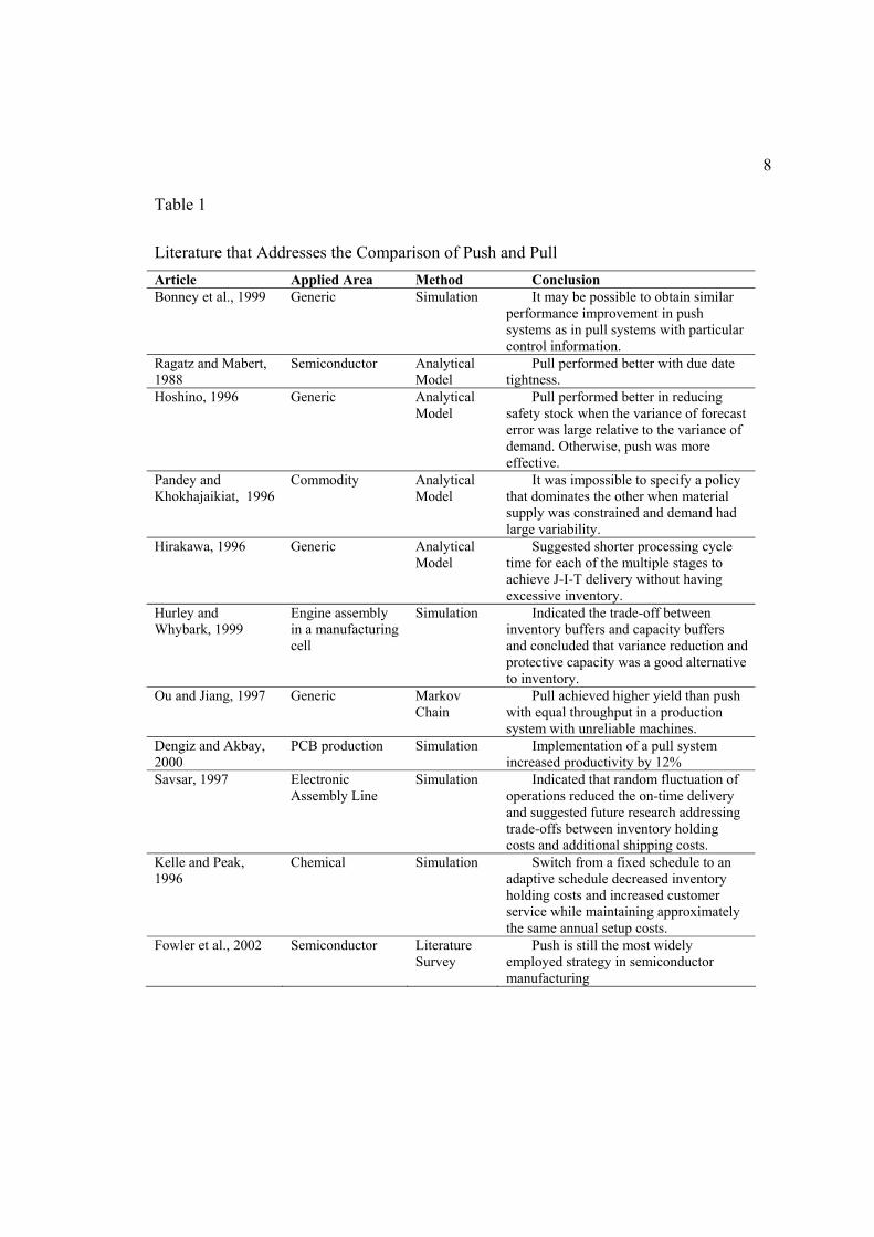
push and pull production systems. Table 1 summarizes the area of application, the
method used and the conclusion drawn in selected papers.
8
Table 1
Literature that Addresses the Comparison of Push and Pull Article Applied Area Method Conclusion Bonney et al., 1999 Generic Simulation It may be possible to obtain similar
performance improvement in push systems as in pull systems with particular control information.
Ragatz and Mabert, 1988
Semiconductor Analytical Model
Pull performed better with due date tightness.
Hoshino, 1996 Generic Analytical Model
Pull performed better in reducing safety stock when the variance of forecast error was large relative to the variance of demand. Otherwise, push was more effective.
Pandey and Khokhajaikiat, 1996
Commodity Analytical Model
It was impossible to specify a policy that dominates the other when material supply was constrained and demand had large variability.
Hirakawa, 1996 Generic Analytical Model
Suggested shorter processing cycle time for each of the multiple stages to achieve J-I-T delivery without having excessive inventory.
Hurley and Whybark, 1999
Engine assembly in a manufacturing cell
Simulation Indicated the trade-off between inventory buffers and capacity buffers and concluded that variance reduction and protective capacity was a good alternative to inventory.
Ou and Jiang, 1997 Generic Markov Chain
Pull achieved higher yield than push with equal throughput in a production system with unreliable machines.
Dengiz and Akbay, 2000
PCB production Simulation Implementation of a pull system increased productivity by 12%
Savsar, 1997 Electronic Assembly Line
Simulation Indicated that random fluctuation of operations reduced the on-time delivery and suggested future research addressing trade-offs between inventory holding costs and additional shipping costs.
Kelle and Peak, 1996
Chemical Simulation Switch from a fixed schedule to an adaptive schedule decreased inventory holding costs and increased customer service while maintaining approximately the same annual setup costs.
Fowler et al., 2002 Semiconductor Literature Survey
Push is still the most widely employed strategy in semiconductor manufacturing
9
Despite the extensive literature that discusses the advantages of a pull strategy in
achieving better operations with simulation and analysis results, this knowledge does not
appear to be common in the boardroom in the semiconductor industry. It is still the push
strategy that semiconductor companies usually implement. The push approach and the
seeming protection of large WIP have not been easily overcome in this industry, even in
companies purporting to adopt J-I-T philosophies (Fowler et al. 2002). What the industry
learned from the most recent downturn is that time and availability rather than technology
are becoming the first priority driver (Shunk et al. 2002). In the recent major downtown,
on-time delivery appears to become more and more important for semiconductor
companies to survive, while the industry’s delivery performance today is not good. A
good example is that Gateway punished Intel by shifting business to AMD in response to
Intel’s poor delivery service (Read 2002). Considering the trade-off between inventory
and service, there is no dominating conclusion that can be cited directly for identifying a
semiconductor supply chain strategy to perform better on cost saving and service
improvement especially under the reality of unpredictable demand and unstable processes.
A hybrid push-pull semiconductor supply chain with a die-bank was recommended
by i2 (2002) for the next generation of production for high-margin, high-volume
semiconductor products to take advantage of both push and pull strategies. The die-bank
sits between the front-end, which contains the wafer fabrication and the probe steps, and
the back-end, which contains the assembly and the test steps, as buffer inventory. Lee
(2001) built optimization models for a die-bank push-pull strategy based on different
order release strategies to maximize throughput and minimize process cycle time in front-

10
end, and to maximize on-time delivery and revenue through the back-end. But the model
was not tested due to the lack of data.
Brown et al. (2000) provided a case study regarding different postponement supply
chain strategies implemented at Xilinx. In a product postponement strategy, Xilinx
pushes programmable chips into final product inventory and customers can customize the
chips with specific software after they get them. In a partial process postponement
strategy (still a push strategy), Xilinx produces generic dies in the front-end based on the
aggregate forecast and afterwards decides the back-end production of final products
based on revised demand forecasts. In a die-bank push-pull strategy, the company pushes
the generic parent dies into the die-bank inventory and the parent dies are customized to
create final product chips when demand occurs. Xilinx also implements a combined
strategy with a mix of push and push-pull. Table 2 summarizes the different decision-
making points and inventory buffer points for such strategies. Using a push-pull strategy
allows Xilinx to hold less finished goods, yet still be responsive to its customers. Xilinx
improved their financial performance based on reduced inventory costs.
Table 2
Xilinx’s Supply Chain Strategies (Brown et al. 2000) Strategy Postponement of
decision Inventory at die-bank
Inventory at finished goods
No postponement (Push) O Partial postponement (Push) O O Die-bank push-pull O O Hybrid O O O
11
Die-bank is a very typical push-pull boundary in semiconductor supply chains.
However, there are other possible choices. Some companies hold inventory before the
interconnection process in the wafer fab so that logic portions on the die can be
connected to “program” specific functions when further demand information is updated.
The parent die must be designed specifically for being able to be programmed. Such a
design always leads to a larger die area and consequently leads to a higher cost.
Furthermore, companies can implement a “pure” pull strategy if the long lead time is
acceptable for customers. As for product postponement, the test stage may be the
postponement point so that chips with different estimated performance can be marked as
different final products.
The semiconductor industry is a hundred-billion-dollar (plus) industry and plays a
fundamental role for today’s global economy. Almost all products are becoming more
and more electronic today than they were yesterday. Lately, empirical analysis indicates
that the semiconductor industry is always under stress: either in a “lack for capacity” or a
“lack for sales” position (Shunk et al. 2002). Also, many technological constraints may
be reached in the foreseeable future. How long Moore’s Law (Moore 1965) is going to be
applicable is unknown at present. The technology-driven semiconductor industry has
realized the importance of putting more intelligent control into the supply chain and
manufacturing. The stress is compelling the industry to change. Companies are beginning
to restructure their inventory and capacity buffers and to accelerate their transition from
push to pull. Such a strategic transition requires tremendous organizational support and
cultural transformation (Kempf 2003). However, before the development of detailed
12
control mechanisms, identifying the appropriate supply chain strategy is a more
fundamental issue. This strategic decision will likely be in place throughout the entire
product life cycle, typically 1.5 to 2 years, because a transition in the middle of the cycle
would be costly involving joint work of marketing, production and technology. An
appropriate strategic decision will lead the tactical and operational decisions to achieve
operational excellence.
Huge demand uncertainty always exists in the semiconductor industry. Customer
demand is dependent on product variety, technical specifications, order quantity, required
lead time and final delivery destination. Abundant forms of process variability also exist.
Among them, manufacturing cycle time is a key issue since the semiconductor industry is
very much driven by cycle time (Fowler et al. 1992). Maltz et al. (2001) also indicated
that global logistics, thought not on the “A-list”, has enormous impact on today’s
semiconductor business. A US company can possibly process the wafer in a European fab,
ship them cross the ocean back to the US for probe, have them assembled in a
subcontracted Asian assembly house and ship them all the way back to the US for final
test since the test process has many technical secrets and a company may not want to
outsource it. It could be difficult to achieve on-time delivery service not only for
customers on the other side of the world but also for domestic ones.
In summary, semiconductor supply chain strategies need to be compared under
different scenarios of demand and process dynamics. We cannot handle such a strategic
decision without understanding the demand nature of the products, nor can we do so
without truly understanding the underlying system behavior of the process (Figure 2).
13
The question is not only “what is the right supply chain for your product?”, but “what is
the right supply chain for your process?”
Figure 2 Overlapping responsibilities across product, process, and supply chain characteristics, Adapted from Fine (1998)
1.3. Organization of the Paper
This paper is organized into three chapters. Chapter 1 introduces the problem and
reviews literature that addresses push and pull strategies in semiconductor manufacturing
and supply chains. In Chapter 2, the three semiconductor supply chain strategies are
modeled using discrete event simulation for playing “what-if” games. Structured
simulation experiments are designed to capture different scenarios of input uncertainty
Product Process
Supply Chain
14
and system variability. Impacts of these variables are measured. Finally, summary of the
results leads to a conceptual decision support framework in Chapter 3 that attempts to
guide the choice of semiconductor supply chain strategy with the goal of “optimizing”
both overall production cost and on-time delivery service. Possible future research is also
suggested. Please note that the organization of this paper leads to some redundant content
between chapters.

Chapter 2
Comparing Semiconductor Supply Chain Strategies under Demand Uncertainty
and Process Variability
2.1. Abstract
A fundamental issue in designing a semiconductor supply chain is to identify the
strategy under which it will operate. Supply chain strategies can be generally categorized
as push, push-pull and pull. In this research we use simulation models and designed
experiments to compare the three strategies under different patterns of demand and
process dynamics. The results indicate that identifying an appropriate strategy is a
consequence of understanding the nature of the demand as well as the systemic behavior
of the process. A conceptual decision support framework is provided following the
analysis that can be used in the selection from push, push-pull and pull semiconductor
supply chain strategies that seeks to optimize the overall production cost and on-time
delivery service under demand uncertainty and process variability.
Keywords: Semiconductor Supply Chain; Push/Pull Strategy; Discrete Event
Simulation; Design of Experiments; Decision Support
2.2. Introduction
This research is driven by the problem of identifying appropriate supply chain
strategies for certain semiconductor products. As supply chain concerns are now on the
16
executive’s radar screen (Maltz et al. 2001), such problem has become a fundamental
issue in the hundred-billion-dollar (plus) semiconductor industry, which provides
building blocks for today’s global information economy.
Regardless of the embarrassment of answering the question “what is the right supply
chain for your product”, we consider the well-known, concise framework provided by
Fisher (1997) as the starting point. The nature of the demand of the product, generally
categorized as being either primarily functional or primarily innovative, drives the
decision. Semiconductors are perfect examples of innovative products with unpredictable
demand and short product lifecycles (Maltz et al. 2001). Thus, a market-responsive
supply chain is suggested to be generally more appropriate than a physically efficient one
according to Fisher (1997).
The semiconductor industry is highly capital intensive and is characterized by high
customer expectations, short product life cycles, proliferating product variety,
unpredictable demand, long and variable manufacturing cycle times, globally distributed
logistics, and considerable supply chain complexity. On one hand, companies try to
maximize the utilization of the facilities under multi-million dollar weekly depreciation;
on the other hand, companies try to build in more responsiveness to the market. Not only
the nature of the product demand but also the underlying system behavior of the entire
semiconductor processes matters. Eventually it is important for operation executives to
understand the overlapping responsibility of product, process and supply chain (Figure 2)
to answer the question “what is the right supply chain for your semiconductor?”

17
Lee et al. (2002) indicated that the goal of supply chain performance management is
to have increased customer service and reduced costs. Thus, a “right supply chain” is
intended to perform well on both cost and service from an operations’ perspective. Today,
chip customers are so insisting on better service, especially on-time delivery performance
(Maltz et al. 2001). Having the latest, fastest chip is not the only key to competition.
Performing better in the two major supply chain performance metrics will lead to
operational excellence and ultimately to competitive advantage. Note that quality is
absent here; in modern Supply Chain Management thinking, quality is always taken as a
given (Hausman 2002).
Notwithstanding many approaches to naming supply chain strategies, integrated
supply chain strategies can be categorized simply as push, pull and hybrid push-pull
systems (Figure 1). The semiconductor supply chain contains sequential manufacturing
stages of wafer fabrication, probe, assembly and test. The die-bank sits between the front-
end (wafer fabrication and probe) and the back-end (assembly and test) to store the
silicon wafers with produced semiconductor dies on them. In the push strategy,
semiconductors are built-to-stock to final products. In the push-pull strategy, wafers with
generic parent dies are produced in the front-end and pushed into die-bank inventory.
When demand occurs the parent dies are pulled from die-bank inventory and assembled-
to-order in the back-end to create different final products. There are many forms of
hybrid push-pull strategies in today’s semiconductor businesses. However, we consider
the state-of-the-art die-bank push-pull approach as the delegate. In the pull strategy,

18
production is not started until real demand occurs, thus semiconductor devices are built-
to-order.
The challenge is to establish generic procedures for identifying appropriate supply
chain strategy transferable across semiconductor businesses. As Aitken et al. (2003)
commented on such problems, we can see how conceptual frameworks, such as the one
of Fisher (1997), work in practice, but figuring out how they work in theory is still of
critical importance because without a suitable model, establishing generic properties in
the dynamic semiconductor businesses becomes extremely difficult. In this research we
attempt an analytic model to capture the basic elements of demands and processes in a
supply chain context to compare these three generic semiconductor supply chain
strategies. The comparative analysis leads to a conceptual decision support framework
which attempts to guide the selection of the semiconductor supply chain strategy with the
goal of “optimizing” overall production cost and on-time delivery service under demand
and process dynamics.
2.3. Literature Review
In this section we start with a general discussion of the terms push and pull, followed
by an overview of literature that addresses the comparison of push and pull in production
systems. Some state-of-the-art approaches to the push-pull semiconductor supply chain
strategy, as well as the latest empirical analysis in the semiconductor supply chain, are
also discussed.

19
A push supply chain makes production and distribution decisions based on forecasts
and a pull supply chain drives production and distribution by customer demand (Simchi-
Levi et al., 2003). However, we need to understand the connection between the push/pull
supply chain strategies and the order release strategies in production systems.
Formal definitions for push and pull production systems at the conceptual level are
provided by Hopp and Spearman (2000). A push system schedules the release of work
based on demand, while a pull system authorizes the release of work based on system
status. Note that the demand placed on the factories is not always the true customer
demand. In many cases, companies make the production plan based on forecasts and
place either an internal order to the enterprise’s own factory or an external order to a third
party manufacturer/foundry so that products are “built-to-stock” and pushed into the
inventory in the push portion of the supply chain. Planned lots may or may not be
released immediately to the factory’s shop floor control domain at the scheduled time.
The system status is a real-time signal that drives the release of the work if the factory
runs a mainly pull philosophy. In the pull supply chain portion, true customer orders
(which drive the production and distribution) are real-time signals. In essence, the
push/pull supply chain system and the push/pull production system share the same
philosophy. In production systems push approaches are driven by what one desires to
produce and pull approaches are driven by what one is capable of producing (Fowler et al.
2002). In supply chains the companies “push” what they desire to sell and “pull” what
they are capable to sell. The essential context is to match the demand with the supply.
20
One produces what are to be sold. One cannot sell what one is not capable of producing
nor can one sell to nonexistent demand.
In the context of matching the demand with the supply, demand uncertainty causes
major problems in the company’s supply chain operations. This uncertainty is amplified
as it moves upstream in the supply chain; this is the “bullwhip effect” described by Lee et
al. (1997). Also the variability within the system is detrimental to system performance.
For example, the fuzzy line between the production plan domain and the shop floor
control domain, discussed in the last paragraph, sometimes is a major cause of the
difficulties in production control (Fowler et al. 2002). There are many forms of
variability, but increasing variability always degrades the performance of a production
system. To reduce its impact, variability is buffered by some combination of inventory,
capacity and time (Hopp and Spearman 2000). Companies have been making efforts to
transition from push to pull for more than 20 years. The transition has, in general, been
focused on reducing inventory buffers but increasing capacity buffers (Schwarz 2003).
By separating the concepts of push and pull from their specific implementations, it is
observed that most real-world systems are actually hybrids or mixtures of push and pull
(Hopp and Spearman 2000). The hybrid push-pull supply chain strategy pushes the goods
into an inventory buffer somewhere in the middle of the entire supply chain awaiting real
demands to drive the pull processes. Ultimately, any supply chain system can be
considered a push-pull system; it just depends on where the push-pull boundary is. If the
boundary is at the beginning of the total process, it is a pull system; at the end, push.
21
No significant body of published research appears to exist addressing push/pull
semiconductor supply chains. However, numerous articles had been published focusing
on push/pull production systems in semiconductor manufacturing and most of them
focused on the wafer fabrication process. Manufacturers implementing a push strategy
simply release all the orders into the factory with MRP methods. Some of them limit
daily release to a fixed quantity based on production goals to avoid excessive WIP (still a
push philosophy). In the 1980s companies realized the lack of intelligent control and
attempted to move to pull philosophies such as J-I-T (Monden 1983) or Kanban (Kimura
and Treda 1981, Mitra and Mitrani 1990, Sugimori et al. 1977). Such efforts were
followed by increased interest in bottleneck methods based on the theory of constraints
(Jacobs 1991). The CONWIP method (Spearman et al. 1990), which targeted the control
of WIP rather than the control of throughput, was also given much attention much
recently. (Fowler et al. 2002)
Are push and pull really so different (Bonney et al., 1999)? In the literature, there has
been considerable interest in the comparison of push and pull systems. Many studies have
been conducted with a variety of environmental considerations to compare and analyze
push and pull production systems. Table 1 summarizes the area of application, the
method used and the conclusion drawn in selected papers.
Despite the extensive literature that discusses the advantages of a pull strategy in
achieving better operations with simulation and analysis results, this knowledge does not
appear to be common in the boardroom in the semiconductor industry. It is still the push
strategy that semiconductor companies usually implement. The push approach and the
22
seeming protection of large WIP have not been easily overcome in this industry, even in
companies purporting to adopt J-I-T philosophies (Fowler et al. 2002). What the industry
learned from the most recent downturn is that time and availability rather than technology
are becoming the first priority driver (Shunk et al. 2002). In the recent major downtown,
on-time delivery appears to become more and more important for semiconductor
companies to survive, while the industry’s delivery performance today is not good. A
good example is that Gateway punished Intel by shifting business to AMD in response to
Intel’s poor delivery service (Read 2002). Considering the trade-off between inventory
and service, there is no dominating conclusion that can be cited directly for identifying a
semiconductor supply chain strategy to perform better on cost saving and service
improvement especially under the reality of unpredictable demand and unstable processes.
A hybrid push-pull semiconductor supply chain with a die-bank was recommended
by i2 (2002) for the next generation of production for high-margin, high-volume
semiconductor products to take advantage of both push and pull strategies. The die-bank
sits between the front-end, which contains the wafer fabrication and the probe steps, and
the back-end, which contains the assembly and the test steps, as buffer inventory. Lee
(2001) built optimization models for a die-bank push-pull strategy based on different
order release strategies to maximize throughput and minimize process cycle time in front-
end, and to maximize on-time delivery and revenue through the back-end. But the model
was not tested due to the lack of data.
Brown et al. (2000) provided a case study regarding different postponement supply
chain strategies implemented at Xilinx. In a product postponement strategy, Xilinx

23
pushes programmable chips into final product inventory and customers can customize the
chips with specific software after they get them. In a partial process postponement
strategy (still a push strategy), Xilinx produces generic dies in the front-end based on the
aggregate forecast and afterwards decides the back-end production of final products
based on revised demand forecasts. In a die-bank push-pull strategy, the company pushes
the generic parent dies into the die-bank inventory and the parent dies are customized to
create final product chips when demand occurs. Xilinx also implements a combined
strategy with a mix of push and push-pull. Table 2 summarizes the different decision-
making points and inventory buffer points for such strategies. Using a push-pull strategy
allows Xilinx to hold less finished goods, yet still be responsive to its customers. Xilinx
improved their financial performance based on reduced inventory costs.
Die-bank is a very typical push-pull boundary in semiconductor supply chains.
However, there are other possible choices. Some companies hold inventory before the
interconnection process in the wafer fab so that logic portions on the die can be
connected to “program” specific functions when further demand information is updated.
The parent die must be designed specifically for being able to be programmed. Such a
design always leads to a larger die area and consequently leads to a higher cost.
Furthermore, companies can implement a “pure” pull strategy if the long lead time is
acceptable for customers. As for product postponement, the test stage may be the
postponement point so that chips with different estimated performance can be marked as
different final products.
24
The semiconductor industry is a hundred-billion-dollar (plus) industry and plays a
fundamental role for today’s global economy. Almost all products are becoming more
and more electronic today than they were yesterday. Lately, empirical analysis indicates
that the semiconductor industry is always under stress: either in a “lack for capacity” or a
“lack for sales” position (Shunk et al. 2002). Also, many technological constraints may
be reached in the foreseeable future. How long Moore’s Law (Moore 1965) is going to be
applicable is unknown at present. The technology-driven semiconductor industry has
realized the importance of putting more intelligent control into the supply chain and
manufacturing. The stress is compelling the industry to change. Companies are beginning
to restructure their inventory and capacity buffers and to accelerate their transition from
push to pull. Such a strategic transition requires tremendous organizational support and
cultural transformation (Kempf 2003). However, before the development of detailed
control mechanisms, identifying the appropriate supply chain strategy is a more
fundamental issue. This strategic decision will likely be in place throughout the entire
product life cycle, typically 1.5 to 2 years, because a transition in the middle of the cycle
would be costly involving joint work of marketing, production and technology. An
appropriate strategic decision will lead the tactical and operational decisions to achieve
operational excellence.
Huge demand uncertainty always exists in the semiconductor industry. Customer
demand is dependent on product variety, technical specifications, order quantity, required
lead time and final delivery destination. Abundant forms of process variability also exist.
Among them, manufacturing cycle time is a key issue since the semiconductor industry is

25
very much driven by cycle time (Fowler et al. 1992). Maltz et al. (2001) also indicated
that global logistics, thought not on the “A-list”, has enormous impact on today’s
semiconductor business. A US company can possibly process the wafer in a European fab,
ship them cross the ocean back to the US for probe, have them assembled in a
subcontracted Asian assembly house and ship them all the way back to the US for final
test since the test process has many technical secrets and a company may not want to
outsource it. It could be difficult to achieve on-time delivery service not only for
customers on the other side of the world but also for domestic ones.
In summary, semiconductor supply chain strategies need to be compared under
different scenarios of demand and process dynamics. We cannot handle such a strategic
decision without understanding the demand nature of the products, nor can we do so
without truly understanding the underlying system behavior of the process (Figure 2).
The question is not only “what is the right supply chain for your product?”, but “what is
the right supply chain for your process?”
26
2.4. Modeling and Analysis
2.4.1. Modeling Considerations and Assumptions
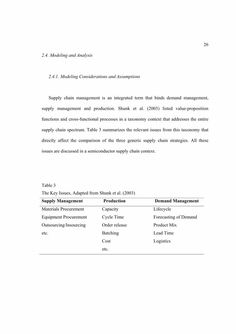
Supply chain management is an integrated term that binds demand management,
supply management and production. Shunk et al. (2003) listed value-proposition
functions and cross-functional processes in a taxonomy context that addresses the entire
supply chain spectrum. Table 3 summarizes the relevant issues from this taxonomy that
directly affect the comparison of the three generic supply chain strategies. All these
issues are discussed in a semiconductor supply chain context.
Table 3
The Key Issues, Adapted from Shunk et al. (2003)
Supply Management Production Demand Management
Materials Procurement
Equipment Procurement
Outsourcing/Insourcing
etc.
Capacity
Cycle Time
Order release
Batching
Cost
etc.
Lifecycle
Forecasting of Demand
Product Mix
Lead Time
Logistics

27
Everything starts with a forecast. There is sometimes confusion between two kinds of
forecasting: “what can be sold (WCBS)” and “what will be sold (WWBS)” (Montgomery
et al. 1990). The former represents possible market trends and unrestricted sales. The
latter always represents the company’s capacity, budget constraints and sales target.
Since capacity utilization is extremely important in the semiconductor industry, it is
always the WWBS forecast that triggers production. In this research two general demand
patterns are modeled: either ‘lack-for-sales’ (WCBS < WWBS) or ‘lack-for-capacity’
(WCBS > WWBS) (Figure 3.).
Figure 3 Demand patterns
Other demand factors are due-date lead time requirements and the mix of products.
Customers can possibly require a tight due-date lead time of several days as well as a
loose one of several weeks. As for product mix, in this research we consider a general
situation with two final products made from one single parent die. It is very common that
companies build parent dies in the front-end and assemble them in different packages to
fit different environmental requirements such as temperature, humidity and pressure. For
WWBS WCBS (Lack-for-capacity)
WCBS (Lack-for-sales)
t
Quantity
28
example, the same microprocessor used for laptop and for desktop computers are put into
different packages. Similar products for commodity and for military usage may have
differently required packages. The packaging costs for each final product are assumed to
be different. We also assume that each final product has an independent demand. As is
often the case, we assume that the cheaper product has higher demand volume and the
more expensive product has lower demand volume.
It is likely that all future semiconductor manufacturing facilities will be 300mm
production lines (TSMC 2002). One 300mm wafer can generate more than twice the
chips that a 200mm wafer produces. Our research focuses on 300mm wafer
manufacturing.
In our research, wafers are released in a lot size of 13, which is feasible for 300mm
wafer production (Seligson 1998). With laser technology, today’s wafers can be marked
with wafer identification numbers (wafer-ID’s) rather than lot-ID’s, therefore customer
orders can be satisfied with units of wafers rather than units of lots. We do not include the
lot-to-order matching issue (Fowler et al. 2000) for simplicity.
Investment in semiconductor manufacturing is beyond the reach of many companies.
More and more companies are running “fabless” today, e.g., Broadcom, NVIDIA,
QUALCOMM, VIA and Xilinx. Nevertheless, a contracted third party manufacturer or
foundry may not perform much different than a company’s own factory from a supply
chain perspective. Companies can freely choose to insource or outsource its fab, probe,
assemble and test processes and the overall supply chain performance should be
measured using many of the same metrics.

29
Without respect to whether the processes are insourced or outsourced, we model the
supply chain as three integrated processes: front-end, back-end and final product delivery
(Figure 4). Two key components of each process are its capacity and its cycle time. A
semiconductor factory always tries to fully utilize its capacity. There are often a large
number of different products running in the factory and they actually compete with each
other for factory resources. Thus, it is difficult to determine the true capacity for a certain
product in such a dynamic environment. Cycle time is a function of capacity and is
becoming a major part of the game. Besides capacity, there are many issues that can
affect the variance of cycle times, e.g., shortage of material, priority in lot release,
priority in scheduling, priority in dispatching, machine breakdown frequency, operator
error, etc. All these factors can also have interaction effects on cycle time. It is almost
impossible for a supply chain executive to have full knowledge of all the details within
the factory even though the company owns the factory or great collaboration is
established between the company and the third-party manufacturer. Therefore we model
the three processes as three “black-boxes” with a single integrated cycle time variability
characteristic.
Figure 4 The “black-box” processes
DeliveryProbeFinal
Goods
Fab Assembly TestDie
Bank Material
Front-end Back-end Delivery

30
In the front-end and the back-end processes, cycle time is the time between releasing
a lot to the factory and releasing the produced wafers to inventory. It is a sum of queueing
time, processing time, moving time and holding time. Note that transportation can also
cause variability since the processes could be globally distributed. Such effects are
modeled in the “black-box” as total cycle time variability.
The final product delivery is almost always performed by a third-party logistics
company (3PL) such as FedEx or UPS (Read 2002). The 3PL will pick up the goods
regularly and deliver to the customer quickly via air. The company may expect a longer
delivery time for specific customer locations. Also regional transportation methods and
traffic conditions can affect the delivery time since the airplanes cannot park at the front
door. A worse situation is that products could be held at customs for several days due to
international trade issues.
2.4.2. Performance Criteria
We measure supply chain performance as a combination of production costs,
inventory costs and service related costs. The key service issue in today’s semiconductor
supply chain is on-time delivery as described previously. Logistics costs are ignored
since semiconductor devices are very small products and the transportation costs are
relatively small.
The production costs can be estimated for certain products (either a per wafer price
charged by the third party foundry or a per wafer cost estimated for the wafers produced

31
in the company’s own factory). The inventory holding costs mainly come from the
opportunity cost of bank interest.
The service performance is put into a penalty cost. Each order has a cited due-date
lead time. If the order misses the cited due date, a penalty is incurred with the amount
based on how long the order is delayed. The penalty per unit time of delay, in essence, is
the weight on service performance that represents the importance of service. A
reasonable example for the penalty is a rebate given back to the customer when the order
delays.
In summery, the following factors need to be analyzed so that we can understand the
impact of demand uncertainty and process variability on semiconductor supply chain
performance under different strategies:
• Demand Factors:
o Demand Pattern (Lack-for-sales or lack-for-capacity)
o Lead Time Requirement
o Importance of On-time Delivery Service
• Process Factors:
o Cycle-time Variability
o Process Costs

32
2.4.3. Description of Simulation Model
Several research studies were conducted with simulation experiments as shown in
Table 1. Simulation modeling facilitates describing the overall supply chain processes,
helps capture the system dynamics with probability distributions, and helps compare
alternatives with “what-if” games in a cost-effective way (Chang and Makatsoris 2001).
The three strategies (push, pull and push-pull) are coded as discrete event simulation
models with Matlab 6.5 R13. Appendix A demonstrates a sample code for a push-pull
scenario.
In our model, forecasts are modeled with ramp-up, steady state, and drop-down stages.
Each stage lasts for 6 months, thus the product lifecycle is 18 months. This is a very
typical semiconductor product lifecycle. On a Pentium 4 - 1.9 GHz personal computer
with 1G RAM, the run-time for each replicate (18 months simulation time) varies from 1
second to 60 seconds depending on how many orders waited in queue for available
inventory.
Large uncertainty of demand exists due to upstream position of semiconductor
devices in the electronics supply chain. The simulation generates random time-between-
arrival (TBA) signals based on the market trends (WCBS forecasting). Order events are
generated based on the TBA signals. Orders are placed in units of wafers. Each order
contains a random quantity of wafers. The aggregate demand per unit time follows a
Poisson distribution. See Figure 3 for the two demand patterns discussed previously. The
low demand, or lack-for-sales scenario, is in essence the situation that demand is below

33
the capacity since the WWBS forecasting mostly represents the capacity. The high
demand, or lack-for-capacity scenario, is the situation that demand surpasses the capacity.
The essential difference between the models is where the inventory is held (i.e., the
location of the push-pull boundary). In the push portion of the system, the simulation
model simply releases works based on WWBS forecasting and generates factory output
events to build inventory after a process delay. (The pull strategy does not have this
portion. The replenishment of the material inventory is the factory’s business). The
inventory is checked when an order event occurs and if the inventory is available, the pull
processes will be activated to fulfill the order (for the push strategy this is the final
product delivery process) and the total lead time is measured. Otherwise, the order is held
in queue awaiting available inventory.
In the push portion, we simply assume that monthly production quantities are planned
based on WWBS forecasting. We also assume that factories operate 24 hours per day,
seven days per week, and 9 lots of the product are released every 8 hours until the
planned monthly quantity is satisfied. Note that the distinction between production plan
and shop floor control is fuzzy. Thus, the factory may or may not release the jobs
immediately as they are scheduled. Cycle time variability affects when each wafer comes
out of the factory and reaches the inventory.
A triangular distribution with “most likely”, “upper bound” and “lower bound” values
is suggested to model the semiconductor manufacturing cycle time characteristics (Duarte
2002). However we model the three integrated process cycle times with larger ranges of

34
variability than that was given in Duarte (2002) (see Table 4). The typical process has a
cycle time in between no variability and such big variability.
Table 4
High Variability Cycle Time Distribution in the Semiconductor Supply Chain Process Min Most Likely Max Mean
Front-end 35 45 55 45
Back-end 5 7 12 8
Final Product Delivery 2 3 7 4
Note: time is in days
The current 300mm raw wafer purchase price is about $400 per wafer. This
contributes to about 12% of $3200 front-end wafer processing cost (Seligson 1998). The
cost varies considerably for different IC designs and process technologies. It could be a
per-wafer production price charged by the outsourced foundry if the company runs
fabless or a per-wafer cost estimated for the company’s own factory. The back-end cost
varies based on the packaging technology. For instance, the assembly and test cost for
Intel’s FCPGA Pentium 4 microprocessor is around $8 (IC Knowledge 2003). One
300mm wafer can generate about 400 dies of such product. Thus, total back-end cost per
wafer is about $3200. This is quantitatively in the same scale as the front-end cost. In this
research, we consider a range of cost as shown in Table 5 following the illustrated cost
model provided by IC Knowledge (2003). Note that the delivery cost is ignored.
35
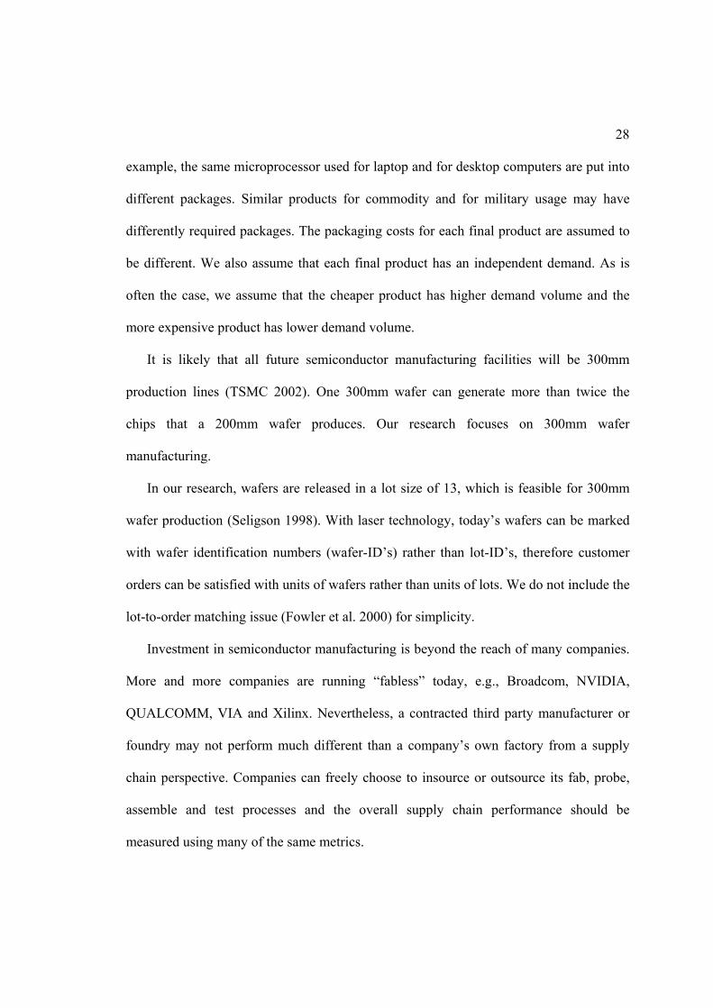
Table 5
Cost Structure Example Portion Low Cost High Cost
Front-end 2400 4000
Back-end for Commodity Goods 2400 4000
Back-end for Military Goods 4800 8000
Note: cost is in US dollar per wafer
Table 6 shows the service penalties based on different cited due-date lead times in our
model.
Table 6
Service Penalty vs. Due-Date Lead Time Level 1: Tight Level 2: Medium Level 3: Loose Due-date Lead Time or
Cited Lead Time 5 days 30 days 55 days Light Penalty
$55 $30 $5 Penalty per delayed hour Heavy
Penalty $275 $150 $25
The total inventory cost throughout the product life cycle is:
∫ ⋅⋅⋅=t
dttevelInventoryLWaferCostInterestostInventoryC )(
The penalty cost for each order is calculated as a weighted tardiness:
),0max( imeCitedLeadTLeadTimeTardiness −=
P = Penalty per unit time of delay
TardinessPtPenaltyCos ⋅=

36
The total penalty cost and the inventory cost are shared by each of the sold wafers. In
the push model, the total manufacturing cost is shared by all the sold wafers. Thus, the
overall cost per wafer sold in the push model is calculated as:
soldwafersNumber
tPenaltyCosostInventoryCtBackendCosstFrontendCoC orderproducedwafer
__
)(_
∑∑ +++=
In the push-pull model Product A and B share the same generic parents die in the die-
bank inventory. Only the total front-end manufacturing cost is shared by all the sold
wafers. The back-end cost is added only for each sold wafer. The overall cost per wafer
sold in the push-pull model is calculated as:
tBackendCossoldwafersNumber
tPenaltyCosostInventoryCstFrontendCoC orderproducedwafer +
++=
∑∑__
_
In the pull model the manufacturing costs is added for each sold wafer. The overall
cost per wafer sold in the pull model is calculated as:
tBackendCosstFrontendCosoldwafersNumber
tPenaltyCosC order ++=
∑__
2.4.4. Experimental Design and Analysis
The goal of the Design of Experiments (DOE) is to determine the impact of different
factors so that desired information may be gained cost-effectively. Table 7 provides an
overview of the DOE factors used to access the performance of the three strategies under

37
various operating conditions. The experimental design is implemented using Design-
Expert 6 (Montgomery 2001).
Table 7
The DOE Factors
Factors Level 1 Level 2 Level 3
Strategy Pull Push-Pull Push
Due-Date Lead Time Tight * Medium * Loose *
Penalty Weight Light * Heavy *
Demand of Product A Lack-for-sales (Low)** Lack-for-capacity (High)**
Demand of Product B Lack-for-sales (Low)** Lack-for-capacity (High)**
Front-end Cycle Time Variability Zero Variability *** High Variability ***
Back-end Cycle Time Variability Zero *** High ***
Delivery Time Variability Zero *** High ***
Front-end Mfg Cost Low **** High ****
Back-end Cost Product A Low **** High ****
Back-end Cost Product B Low **** High ****
Note: Product A and Product B are two final products packaged from the same parent die. * Use the data in Table 6 ** See Figure 3 for demand patterns. *** Use the triangular distribution in Table 4 as high variability. Use the mean
value as Zero variability **** Use the data in Table 5
Note that we have both 3-level factors and 2-level factors. We use two 2-level factors
to represent one 3-level factor. Thus, there are 13 factors and a 5132 − fractional factorial
design of experiments is conducted. This is a Resolution V Design so that no main effect
or two-factor interaction is aliased with any other main effect or two-factor interaction
(Montgomery 2001). Figure 5 is a Half Normal Plot for the results of this experiment for

38
Product A. The factors and interactions that are significant are the ones that are not on the
line. There are many significant terms. Wan et al. (2003) suggested a sequential
bifurcation analysis for simulation experiments since in simulation most of the factors
have some effects. Factors are grouped as either being important or being unimportant. In
each step only one group of factors is analyzed for importance leaving the other factors
for further step-down analysis. The significant main effects of front-end and back-end
costs are so obvious that we do not need to measure them at this step. Thus, in this global
experiment only the effects of strategy, service penalty, due-date lead time and their
interactions are captured for examination.
Figure 5 Effects of the global experiment
Important Group
Unimportant Group
Too obvious
Total cost per wafer sold -Product A
39
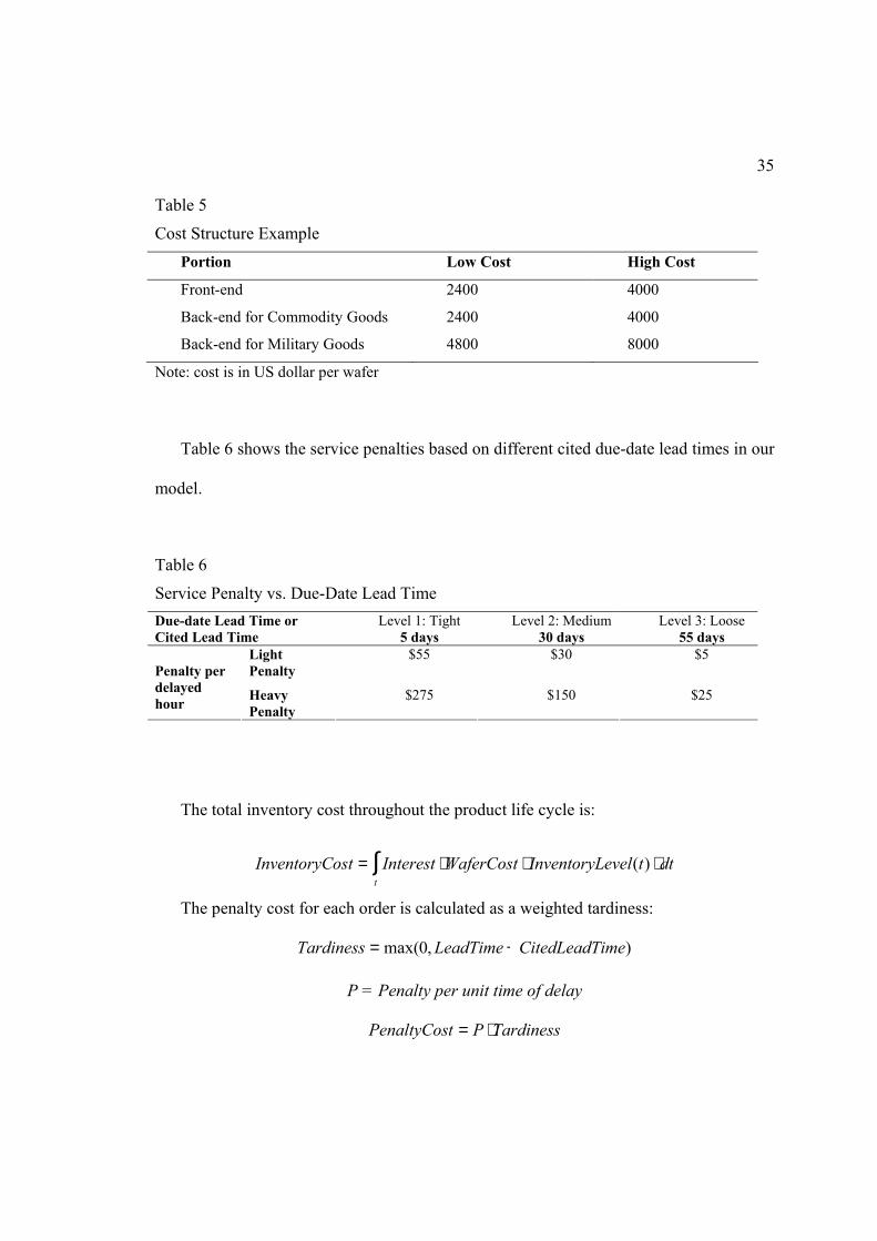
Therefore, the responses of total cost per wafer sold of Product A are examined under
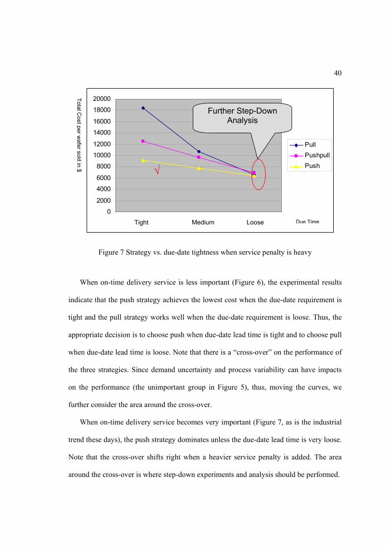
different patterns of due-date requirement and service penalty. Figure 6 and Figure 7
show the results of the three strategies under different due-date tightness. Figure 6 is the
results when service penalty is light; Figure 7, heavy.
Figure 6 Strategy vs. due-date tightness when service penalty is light
0
2000
4000
6000
8000
10000
12000
1 2 3
PullPushpullPush
Tight Medium Loose Due TimeTotal C
ost per wafer sold in $
Further Step-Down Analysis
√ √
40
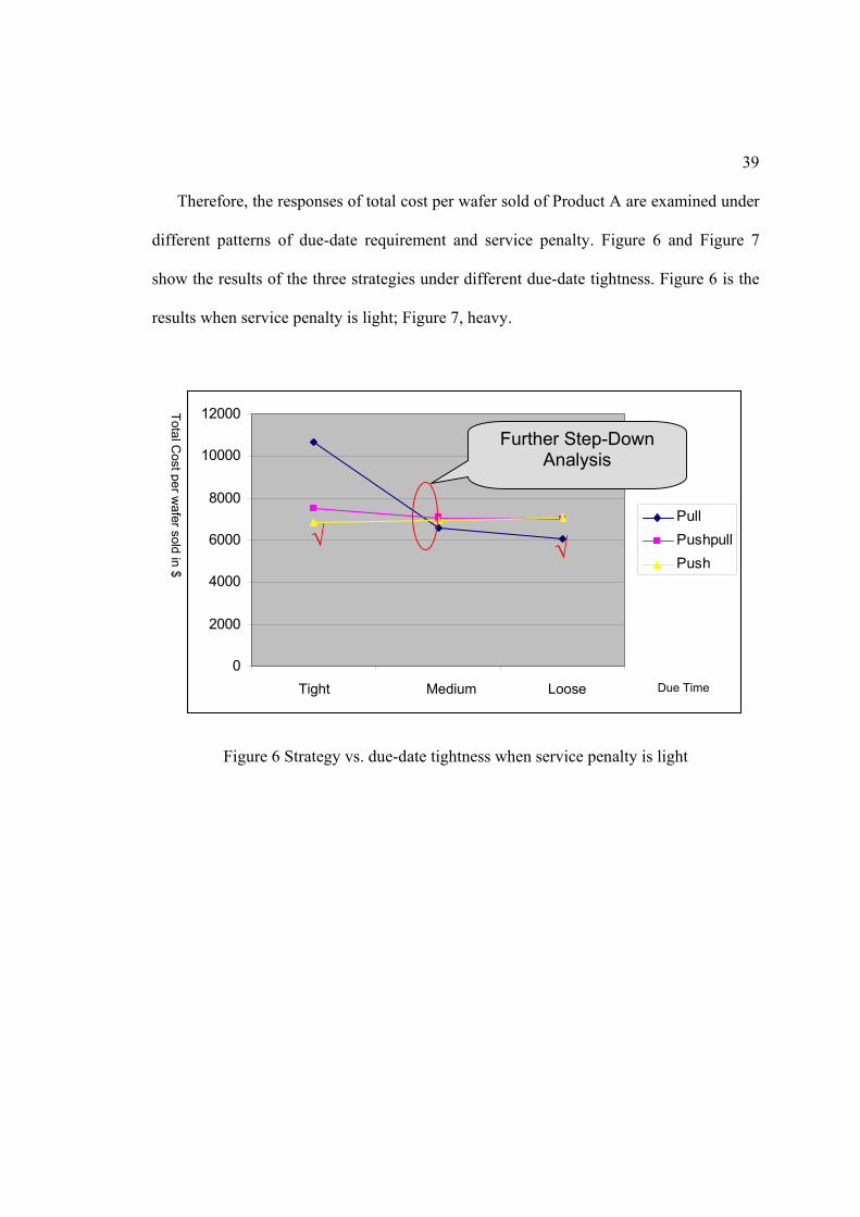
Figure 7 Strategy vs. due-date tightness when service penalty is heavy
When on-time delivery service is less important (Figure 6), the experimental results
indicate that the push strategy achieves the lowest cost when the due-date requirement is
tight and the pull strategy works well when the due-date requirement is loose. Thus, the
appropriate decision is to choose push when due-date lead time is tight and to choose pull
when due-date lead time is loose. Note that there is a “cross-over” on the performance of
the three strategies. Since demand uncertainty and process variability can have impacts
on the performance (the unimportant group in Figure 5), thus, moving the curves, we
further consider the area around the cross-over.
When on-time delivery service becomes very important (Figure 7, as is the industrial
trend these days), the push strategy dominates unless the due-date lead time is very loose.
Note that the cross-over shifts right when a heavier service penalty is added. The area
around the cross-over is where step-down experiments and analysis should be performed.
0
2000
4000
6000
8000
10000
12000
14000
16000
18000
20000
1 2 3
PullPushpullPush
Tight Medium Loose Due Time
Total Cost per w
afer sold in $ √
Further Step-Down Analysis

41
Two sets of step-down experiments are conducted.
• Set 1: Penalty = Light; Lead Time = 4 weeks
• Set 2: Penalty = Heavy; Lead Time = 8 weeks
All other factors remain the same. Two 2102 − experiments (Resolution VI Design) are
designed and implemented, still having two 2-level factors representing each 3-level
factor. Figure 8 clearly shows the factorial effects of Set 1 experiments.
Figure 8 Effects of the step-down experiments
The factorial effects of Set 2 experiments are very similar as those of Set 1 (Handling
in Figure 8). The most significant effects are main effects of costs. Again, we do not need
Total Cost per Wafer Sold – Product A
Strategy
42
to analyze them since they are obvious. Demand pattern (2-factor-interaction of EF in
Figure 8) and cycle time variability (main effect of C as well as interaction of CDJ in
Figure 8) appear to be important. Note that the 2-factor-interaction of the demand pattern
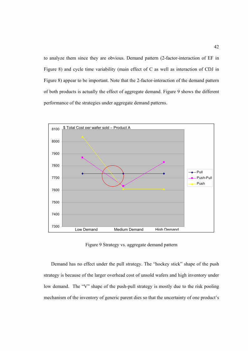
of both products is actually the effect of aggregate demand. Figure 9 shows the different
performance of the strategies under aggregate demand patterns.
Figure 9 Strategy vs. aggregate demand pattern
Demand has no effect under the pull strategy. The “hockey stick” shape of the push
strategy is because of the larger overhead cost of unsold wafers and high inventory under
low demand. The “V” shape of the push-pull strategy is mostly due to the risk pooling
mechanism of the inventory of generic parent dies so that the uncertainty of one product’s
7300
7400
7500
7600
7700
7800
7900
8000
8100
PullPush-PullPush
Low Demand Medium Demand High Demand
$ Total Cost per wafer sold – Product A

43
demand can be reduced by another’s. Note that the service weight and due-date are the
dominate drivers. The exact positions of the cross-over can be shifted based on how the
service penalty and due-date requirements are picked.
The large impact of cycle time variability (main effect of C as well as the interaction
of CDJ) cannot be deciphered clearly in this step of analysis. Thus, we establish further
step-down analysis to gain more detailed information.
Further step-down experiments are implemented to address the effects for the push,
push-pull and pull strategies separately. Figure 10 shows the effects of the push strategy
when it is a dominating or possible strategy.

44
Figure 10 The push effects – product A
Demand pattern (main effect of C in Figure 10) has a negative impact on overall cost
(makes performance worse) when service requirements are “tougher” (tighter due-date,
heavier penalty). Many penalties are added when the demand is high. Such impact turns
out to be positive (makes performance better), discussed following Figure 9, when
service requirements become “easier” (around the cross-overs of Figures 6 and 7) and
most of the orders can be caught up without delays under the push strategy. Demand
Heavy Penalty
n/a Push is not chosen here.
Light Penalty
Factors: A: FTime B: BTime C: Dmd A D: Dmd B E: Deliv T F: FCost G: BCostA H: BCostB Designs
Loose Due-Date Lead Time
Medium Due-Date Lead Time
Tight Due-Date Lead Time
Push Effects Product A
282 −

45
pattern and back-end variability can have an interaction effect under tougher service
requirements (refer to the interaction of BC in Figure 10). The back-end variability has a
positive impact on cost performance when demand is high (Figure 11). Such impact is
overcome by the main effect of the demand pattern when service requirements become
easier and the positive impact of demand pattern becomes more important.
0
2000
4000
6000
8000
10000
12000
Demand is LowDemand is High
Figure 11 Interactive effect of demand pattern and back-end variability for push
The push-pull strategy is also tested with a medium due-date lead time and a light
penalty as well as with a loose due-date and a heavy penalty.
Low Variability HIghVariability

46
Figure 12 The push-pull effects
Front-end variability can have a positive impact when due-dates are medium. Such
effect becomes less important when due-dates are loose. The aggregate demand, rather
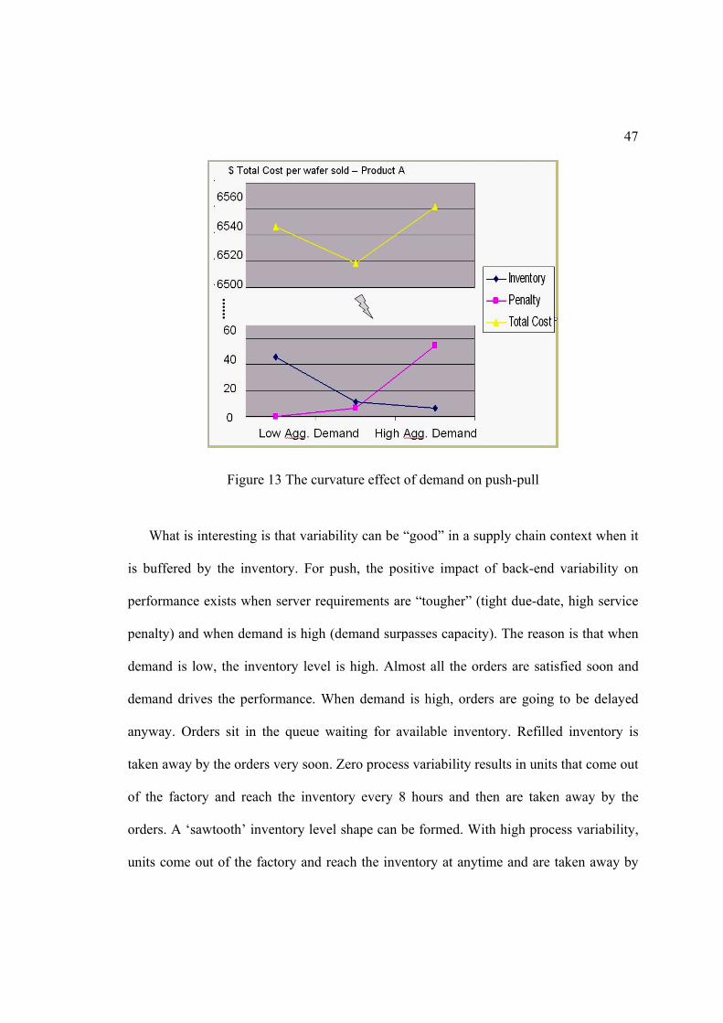
than the independent demand, has a significant curvature effect. The risk-pooling effect
of the push-pull strategy is dramatic as shown. The trade-off between inventory and
service affected by demand is distinctly shown in Figure 13.
n/a
n/a
Heavy Penalty
n/a
Light Penalty
Factors: A: FTime B: BTime C: Dmd A D: Dmd B E: Deliv T F: FCost
Full 62 Designs
Loose Due-Date Lead Time
Medium Due-Date Lead Time
Tight Due-Date Lead Time
Push-pull Effects Product A/B
47
Figure 13 The curvature effect of demand on push-pull
What is interesting is that variability can be “good” in a supply chain context when it
is buffered by the inventory. For push, the positive impact of back-end variability on
performance exists when server requirements are “tougher” (tight due-date, high service
penalty) and when demand is high (demand surpasses capacity). The reason is that when
demand is low, the inventory level is high. Almost all the orders are satisfied soon and
demand drives the performance. When demand is high, orders are going to be delayed
anyway. Orders sit in the queue waiting for available inventory. Refilled inventory is
taken away by the orders very soon. Zero process variability results in units that come out
of the factory and reach the inventory every 8 hours and then are taken away by the
orders. A ‘sawtooth’ inventory level shape can be formed. With high process variability,
units come out of the factory and reach the inventory at anytime and are taken away by
......

48
the order almost immediately. This apparently causes a lower mean inventory level. Total
inventory cost is the integration of the inventory level over time multiplying per unit per
time holding cost. Therefore, high process variability can achieve lower inventory cost.
Similarly, front-end variability can have a positive impact on cost performance under the
push-pull strategy since it can cause a smoother die-bank inventory.
The pull strategy is a feasible choice when due dates are loose. Neglecting the
obvious effect of process costs, cycle time variability has a significant negative impact on
cost performance when the due date lead time is greater than six weeks as shown in
Figure 14.
Figure14 Cycle time variability effects on pull
By clearly understanding the impacts of variability when analyzing the push, push-
pull and pull strategies separately, we can aggregate the impact of process variability on
the impact of demand uncertainty to have a more across-the-aboard view for the cross-
6350
6400
6450
6500
6550
6600
6650
CDE
Zero Variability
High Variability
$ Total Cost per wafer sold – Product A
Front-end Variability
Back-end Variability
Delivery Variability
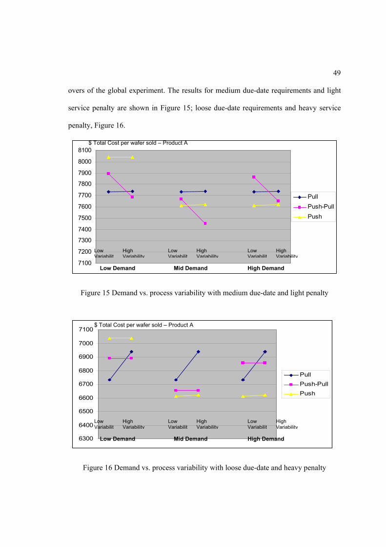
49
overs of the global experiment. The results for medium due-date requirements and light
service penalty are shown in Figure 15; loose due-date requirements and heavy service
penalty, Figure 16.
7100
7200
7300
7400
7500
7600
7700
7800
7900
8000
8100
PullPush-PullPush
Figure 15 Demand vs. process variability with medium due-date and light penalty
6300
6400
6500
6600
6700
6800
6900
7000
7100
PullPush-PullPush
Figure 16 Demand vs. process variability with loose due-date and heavy penalty
$ Total Cost per wafer sold – Product A
Low Demand Mid Demand High Demand
Low Variabilit
High Variability
Low Variabilit
High Variability
Low Variabilit
High Variability
$ Total Cost per wafer sold – Product A
Low Demand Mid Demand High Demand
Low Variabilit
High Variability
Low Variabilit
High Variability
Low Variabilit
High Variability
50
Such results can provide clearer view for choosing appropriate strategy under certain
demand and process patterns.
The previous analysis focused on Product A, which represents the semiconductor
devices for commodity usage. As for Product B, the analytical results indicate that the
effects are clearer. In the global experiment, the most important factors are the same.
Due-date requirements and service penalty are the driving issues. In the step-down
experiment sets, demand always has a large impact under the push strategy since back-
end costs are higher. Therefore, inventory contributes a larger portion to the cost.
Demand and cost have an interaction effect since costs are associated with inventory. The
impact of process variability is (relatively) not very important. Under the push-pull and
the pull strategies, the results for Product B are the same as those for Product A. In our
research, Product B represents more complex parts having higher cost and relatively
larger range of demand. Demand related factors are the issues to be considered for
choosing the supply chain strategy for Product B.
The analysis so far has clearly indicated that by knowing what is important and by
understanding the nature of the demand of the product as well as the underlying system
behavior of the process, proper identification of the semiconductor supply chain
strategies can be accomplished.

51
2.4.5. Validation and Verification
Sterman (2000) indicates that validation and verification of models like ours are
impossible. We are not quite as pessimistic. Verification is mainly debugging work and
in this research our model is simple enough that this is not difficult. As for validation,
extreme situations are tested as boundary adequacy tests. We attempt to use realistic data
in this research representing a general case in the industry. However, more
comprehensive validation testing by consulting with industrial experts to assess the
structure, input terms and output system behavior is desired.
Chapter 3
Conclusions and Future Research
3.1. Conclusions
The analysis of a general case study in the last chapter has clearly indicated that with
enough understanding of the nature of the demand of the product as well as the
underlying system behavior of the process, appropriate identification of the push, push-
pull and pull semiconductor supply chain strategies can be accomplished.
Though continuously improving the quality of information does not necessarily
improve the quality of the decision, we believe that the right information helps
understand the given semiconductor supply chain and helps achieve our goal. Information
availability, per se, demand visibility and supply visibility, is critical for making the
decision. The aggregation of demand and supply information as well as the analysis of
demand and supply information must be performed as this industry matures (Shunk 2003).
This research attempts to provide a conceptual framework to support the decision of
identifying appropriate semiconductor supply chain strategy. Figure 17 shows the first
layer of such a conceptual framework that implicates the driving factors. Lead time
requirements and the importance of on-time delivery services drive the strategic decision
in high priorities.

53
Figure 17 The first layer of the decision support framework
Layer Two consideration is desired for certain situations, specifically for medium
due-dates with low service weights, or loose due-dates with high service weights (cross-
overs in Figures 6 and 7). Table 8 summarizes the decision support framework at this
layer following the analytical results in Figures 15 and 16.
Table 8
Layer Two Framework
Layer Two Low Demand (Lack-for-sales)
Average Demand High Demand (Lack-for-capacity)
Low Mfg* Variability
Pull Push Push
High Mfg* Variability
Push-Pull Push-Pull Push
* Manufacturing variability contains both front-end and back-end variability
Due-Date Lead Time Tight Medium Loose Im
portance of on-time delivery service
Less Important
Far More Im
portant
Push
Pull
Step-down to Layer Two Comparison

54
Such a framework attempts to guide the thinking at the conceptual level rather than to
provide a definitive answer. Furthermore, some implementation issues are necessary to
be paid attention to:
Choosing push: Push works better when the service requirements are “tougher” (tight
due-dates, heavy penalty as in the lower-left corner of Figure 17) as well as when the
demand exceeds the capacity under an “easier” service requirement. From a
manufacturing perspective, variability is always bad. But since it is buffered by the
inventory, maybe the company could tolerate the status quo of the process variability
since reducing variability is never an easy job. When the demand is low (lack-for-sales),
more sales efforts (if the cost is not high) are probably necessary to be addressed to
gather bigger market-share.
Choosing push-pull: Push-pull can work well when the service requirements are not
extremely “tough” and demand is not very high with high front-end cycle time variability.
Again, the large front-end variability is buffered by the die-bank inventory. Demand
uncertainty is better pooled by the generic parent die inventory.
Choosing pull: Pull works when due-dates are loose and service is not very important.
Variability is absolutely bad here. Companies must make efforts to reduce process
variability even though it is a laborious job. Note that it is not unusual that the
semiconductor company runs a billion-dollar business on a certain product. A 5% cost
reduction is intensely noteworthy. Buying more capacity, which could help reduce the
variability, adds the cost so this needs to be carefully studied.

55
Poor delivery service mostly comes from mismatched demand and capacity as well as
from manufacturing process variability. Final product logistics process appears to have
little impact in our study.
Such conclusions are drawn for Product A, as defined in the last chapter representing
high-volume, commodity use semiconductor devices. Our comparison research indicated
that both the nature of the demand and the nature of the process affect the choice of the
semiconductor supply chain strategy. As for Product B, which represents low-volume
complex parts, the demand nature is the driving issue. The decision support framework
guides the direction of thinking. However, sometimes executives may need to access the
probability of being in each case and implement a decision analysis using our framework
to make the choice if it is not sure that in which case their businesses will be. They may
also want to do more detailed analysis to gain more accurate results which can better
support the decision especially at the “cross-overs”.
3.2. Future Research
It is possible to implement some combination of the strategies. For instance, it could
be reasonable for a semiconductor device or electronics component provider to satisfy
“tough” customers, who always place orders with very tight due-date requirements, with
a push strategy, and to satisfy “more friendly” customers with a push-pull or even a pull
strategy if the demand does not exceed the capacity. Real-time information can also
trigger a transition from one strategy to another. However, such a strategic transition may

56
require a lot of work in technology alteration and business process reengineering as well
as tremendous organizational support and cultural transformation. Future research work
can be conducted to address the transition issue. Other push-pull strategies involving
technology complications, such as the strategy that setting the push-pull boundary before
the interconnection process in the wafer fab, can also be studied.
Being aware of the physical relationship between cycle time and capacity, more
detailed simulation modeling with the integrated cycle time–throughput curve could
support better decision making especially at the “cross-overs”. The criticality of detailed
simulation in the semiconductor supply chain is studied by Jain et al. (1999), whereas the
question here is how deep we should go.

REFERENCES
Aitken, J., P. Childerhouse and D. Towill. 2003. The impact of product lifecycle on
supply chain strategy. International Journal of Production Economics 85: 127-140.
Bonney, M.C., Z. Zhang, M.A. Head, C.C Tien and R.J. Barson. 1999. Are push and pull
systems really so different? International Journal of Production Economics 59: 53–
64.
Brown, A.O., H.L. Lee, R. Petrakian. 2000. Xilinx improves its semiconductor supply
chain using product and process postponement. Interfaces 30(4): 65-80.
Chang, Y., and H. Makatsoris. 2001. Supply chain modeling using simulation.
International Journal of Simulation Vol.2 No.1
Dengiz, B. and K.S. Akbay. 2000. Computer simulation of a PCB production line:
metamodeling approach. International Journal of Production Economics 63: 195-205.
Duarte, B.M.. 2002. Parameterization of Fast and Accurate Simulations for Complex
Supply Networks. Master Thesis, Arizona State University
Fine, C.H. 1998. Clockspeed: winning industry control in the age of temporary
advantage. Perseus Books.
Fisher, M.L. 1997. What is the right supply chain for your product. Harvard Business
Review March–April: 105–116.
Fowler, J.W., G.L. Hogg and S.J. Mason. 2002. Workload control in the semiconductor
industry. Production Planning and Control 13(7): 568-578.
Fowler, J.W., K. Knutson and W.M. Carlyle. 2000. Comparison and evaluation of lot-to-
order matching policies for a semiconductor assembly and test facility. International
Journal of Production Research 38(8): 1841-1853.

58
Fowler, J.W., D.T. Phillips and G.L. Hogg. 1992. Real-time control of multi product
bulk-service semiconductor manufacturing processes. IEEE Transactions of
Semiconductor Manufacturing 5(2).
Hausman, W.H. 2002. Supply chain performance metrics. The Practice of Supplhy Chain
Management. Kluwer Academic Publishers.
Hirakawa, Y., 1996. Performance of a multi-state hybrid push/pull production control
system. International Journal of Production Economics 44: 129-135.
Hopp, W.J. and M.L. Spearman. 2000. Factory Physics. Irwin/McGraw-Hill.
Hoshino, K., 1996. Criterion for choicing order policies between fixed-size and fixed
interval, push-type and pull-type. International Journal of Production Economics 44:
91-95.
Hurley, S.F. and D.C. Whybark. 1999. Inventory and capacity trade-offs in a
manufacturing cell. International Journal of Production Economics 59: 203–212.
i2 Technologies. 2002. i2 High Tech Semiconductor Overview and i2 Solutions for the
Semiconductor Industry, available at
http://www.i2.com/solutionsbyindustry/hightech/semiconductor.cfm
IC Knowledge Inc. 2003. 2003 IC Cost Model. Available at
http://www.icknowledge.com/our_products/cost_model.html
Jacobs, F. R. 1984. OPT uncovered. Industrial Engineering 16: 32-35.
Jain, S., C.C. Lim, B.P. Gan and Y.H. Low. 1999. Criticality of Detailed Modeling in
Semiconductor Supply Chain Simulation. Proceeding of the 1999 Winter simulation
conference.

59
Kelle, P. and D. Peak. 1996. A comparison of fixed and adaptive type controls for multi-
product processing. International Journal of Production Economics 45: 139-146.
Kempf, K.G. 2003. Optimization of a semiconductor supply chain: technical and cultural
Issues. Proceedings of INFORMS Conference on OR/MS Practice.
Kimura, O. and H. Terada. 1981. Design and analysis of pull system: a method of multi-
stage production control. International Journal of Production Research 19(3): 241-
253.
Lee, H.L. and J. Amaral. 2002. Continuous and stainable improvement through supply
chain performance management. Stanford Global Supply Chain Management Forum
SGSCMF-W1-2002.
Lee, H.L., V. Padmanabhan and S. Whang. 1997. Information Distortion in a Supply
Chain: The Bullwhip Effect. Management Science 43(4).
Lee, Y.H., 2001. Supply chain model for the semiconductor industry of global market.
Journal of Systems Integration 10(3): 189-206.
Maltz, A.B., W.L. Grenoble, D.S. Rogers, R.M. Baseman, W. Grey and K.K. Katircioglu.
2001. Lessons from the semiconductor industry. Global Supply Chain - an Avnet, Inc.
Publication, Jan: p26-.
Mitra, D.,and I. Mitrani. 1990. Analysis of a kanban discipline for cell coordination in
production lines. Management Science 36(12): 1548-1566.
Monden, Y., 1983. Toyota production system. Industrial Engineering and Management
Press. Norcross, Georgia.
Montgomery, D.C. 2001. Design and Analysis of Experiments 5th Edition. Wiley.

60
Montgomery, D.C., L.A. ohnson and J.S. Gardiner. 1990. Forecasting and Time Series
Analysis 2nd edition. New York: McGraw-Hill.
Moore G.E., 1965. Cramming more components onto integrated circuits. Electronics
April.
Ou, J. and J. Jiang. 1997. Yield comparisons of push and pull control methods on
production systems with unreliable machine. International Journal of Production
Economics 50: 1-12.
Pandey P.C. and P. Khokhajaikiat. 1996. Performance modeling of multistage production
system operating under hybrid push/pull control. International Journal of Production
Economics 43: 17-28.
Ragatz, G.L. and V.A. Mabert. 1988. An Evaluation of order release mechanisms in a
job-shop environment. Decision Sciences 19 (1): 167-189.
Read, J. 2002. The semiconductor supply chain. Global Supply Chain - an Avnet, Inc.
publication. May
Savsar, M. 1997. Simulation analysis for a pull-push electronic assembly line.
International Journal of Production Economics 51: 205-214.
Schwarz, L.B., 2003. Supply-Chain Management: A View of the Future. Lecture Notes,
May.
Seligson, D. 1998. Planning for 300mm transition. Intel Technology Journal Q4'98.
Shunk D.L., 2003. A global test phase plan for establishing globally collaborative supply
network. Working Paper, Arizona State University.

61
Shunk, D.L., J. Carter, J. Hovis and A. Talwar. 2002. The drivers of intermediation and
disintermediation when the industry is under stress. Working paper, Arizona State
University.
Shunk, D.L., Y. Sun, A. Talwar and G. Sandhu. 2003. Establishing communities of
common interest in the US manufacturing society, Working Paper, Arizona State
University.
Simchi-Levi, D., P. Kaminsky and E. Simchi-Levi. 2003. Designing and managing the
supply chain: concepts, strategies, and case studies 2nd edition. McGraw-Hill/Irwin.
Spearman, M.L., D.L. Woodruff and W.J. Hopp. 1990. CONWIP: a pull alternative to
kanban. International Journal of Production Research 28(5): 879-894.
Sterman, J.D. 2000. Business dynamics: systems thinking and modeling for a complex
world. Irwin/McGraw-Hill.
Sugimori, Y.K., F.C. Kusukoki and S. Uchikawa. 1977. Toyota production system and
kanban system: materialisation of just-in-time and respect-for-human system.
International Journal of Production Research 15(6): 564-594.
Taiwan Semiconductor Manufacturing Co. Ltd. (TSMC). 2002. 300mm Wafer
Manufacturing: TSMC's Future. Available at
http://www.tsmc.com/download/enliterature/300mm_bro_2002.pdf
Wan, H., B. Ankenman and B.L. Nelson. 2003. Controlled sequential bifurcation: a new
factor-screening method for discrete event simulation. Proceedings of the 2003
Winter Simulation Conference.

APPENDIX A
SAMPLE CODE FOR PUSH-PULL MODEL

63
%%%%%%%%%%%%%%%%%%%%%%%%%%%%%%%%%%%%%%%%%%%% %This is a sample Matlab code for the %die-bank push-pull %semiconductor supply chain. %Yang Sun all rights reserved 2003 %All variables are global variables. %%%%%%%%%%%%%%%%%%%%%%%%%%%%%%%%%%%%%%%%%%%% % warning off MATLAB:divideByZero % %The experiment code is read in experiment control program. Experiment=[LA(runID)+LB(runID),LC(runID),LD(runID),LE(runID), ... LF(runID), LG(runID),LH(runID),LJ(runID),LK(runID)+LL(runID), ... LM(runID),LN(runID)] Model='push-pull' % %%%%%%%%%%%%%%%%%%%%%%%%%%%%%% %Mfg Release %6-month Ramp-up release(1:17280)=0; day=1081; for i=1:6 num=(i*2-1)*7; k=day; for j=1:num release(k)=9; k=k+8; end day=day+720; end %6-month Steady for i=1:6 num=84; k=day; for j=1:num release(k)=9; k=k+8; end day=day+720; end %6-month Drop-down for i=1:6 num=((7-i)*2-1)*7; k=day; for j=1:num release(k)=9; k=k+8; end day=day+720; end %mfg released %%%%%%%%%%%%%%%%%%%%%%%%%%%%%% % %set the due-date lead time pattern if LK(runID)==0 & LL(runID)==0

64
Due=5; elseif LK(runID)==1 & LL(runID)==1 Due=55; else Due=30; end % loop0=LE(runID)+LF(runID)+1; %set the aggregate demand pattern switch loop0 case 1 topd=7000; case 2 topd=9000; otherwise topd=11000; end % FCost=LJ(runID)*1600+2400; %Front-end cost BCostA=LM(runID)*1600+2400; %Back-end cost product A BCostB=LN(runID)*3200+4800; %Back-end cost product B Pen=(LH(runID)*4+1)*(60-Due); %Penalty per hour per order late % loop4=LC(runID)+1; switch loop4 case 1 %Push-Pull Steady Factory Output mfgout(1:17280)=0; mfgout(2161:15120)=release(1081:14040).*13; otherwise %Push-Pull Random Factory Output mfgout(1:17280)=0; for i=1:14040 if release(i)>0 for j=1:release(i) r=rand(1); if r<=(45-35)/(55-35) delay=round((35+sqrt((45-35)*(55-35)*r))*24); mfgout(i+delay)=mfgout(i+delay)+13; else delay=round((55-sqrt((55-45)*(55-35)*(1- ... r)))*24); mfgout(i+delay)=mfgout(i+delay)+13; end end end end end % loop5=LD(runID)+1; %back-end variability loop6=LG(runID)+1; %delivery variability % for loop10=1:1 % replicates % %%%%%%%%%%%%%%%%%%%%%%%%%%%%%%%%%%%%%%%%%%%%%%%TBA curve
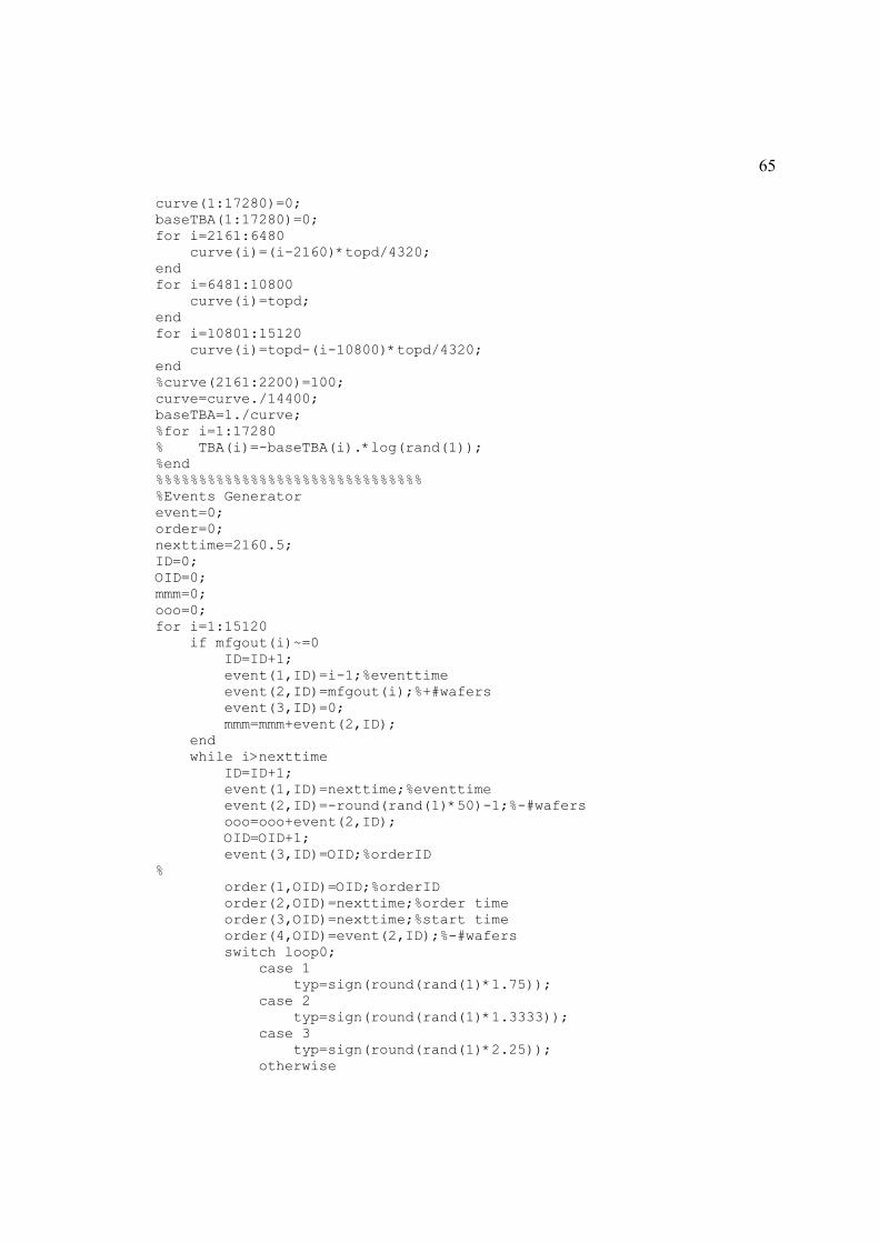
65
curve(1:17280)=0; baseTBA(1:17280)=0; for i=2161:6480 curve(i)=(i-2160)*topd/4320; end for i=6481:10800 curve(i)=topd; end for i=10801:15120 curve(i)=topd-(i-10800)*topd/4320; end %curve(2161:2200)=100; curve=curve./14400; baseTBA=1./curve; %for i=1:17280 % TBA(i)=-baseTBA(i).*log(rand(1)); %end %%%%%%%%%%%%%%%%%%%%%%%%%%%%%%% %Events Generator event=0; order=0; nexttime=2160.5; ID=0; OID=0; mmm=0; ooo=0; for i=1:15120 if mfgout(i)~=0 ID=ID+1; event(1,ID)=i-1;%eventtime event(2,ID)=mfgout(i);%+#wafers event(3,ID)=0; mmm=mmm+event(2,ID); end while i>nexttime ID=ID+1; event(1,ID)=nexttime;%eventtime event(2,ID)=-round(rand(1)*50)-1;%-#wafers ooo=ooo+event(2,ID); OID=OID+1; event(3,ID)=OID;%orderID % order(1,OID)=OID;%orderID order(2,OID)=nexttime;%order time order(3,OID)=nexttime;%start time order(4,OID)=event(2,ID);%-#wafers switch loop0; case 1 typ=sign(round(rand(1)*1.75)); case 2 typ=sign(round(rand(1)*1.3333)); case 3 typ=sign(round(rand(1)*2.25)); otherwise

66
typ=sign(round(rand(1)*1.6667)); end order(5,OID)=typ;%type order(6,OID)=0;%mark % nexttime=nexttime-max(-3000,baseTBA(i)*log(rand(1))); end end %%%%%%%%%%%%%%%%%%%%%%%%%%%%%%%%%%%% %simulation process inv=0; inven=0; que=0; ss=0; sss=0; res=0; len=length(event); for i=1:len if event(2,i)>0 inv=inv+event(2,i); %add inv if the event is a mfg output event % if ss>0 %try to release orders in queue for j=1:ss if inv>-que(4,j) inv=inv+que(4,j); order(3,que(1,j))=event(1,i); order(6,que(1,j))=1; que(1:6,j)=order(1:6,j); % tt(i)=order(3,que(1,j))-order(2,que(1,j)); res=res+1; end end tempque=0; temps=1; for j=1:ss if que(6,j)==0; tempque(1:6,temps)=que(1:6,j); temps=temps+1; end end que=0; que=tempque; ss=ss-res; res=0; end end % if event(2,i)<0 % check inventory for incoming orders inv=inv+event(2,i); % if inv<0 inv=inv-event(2,i); ss=ss+1;
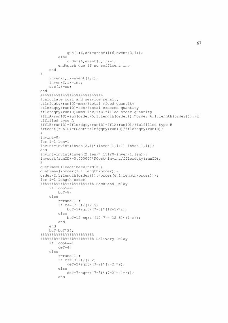
67
que(1:6,ss)=order(1:6,event(3,i)); else order(6,event(3,i))=1; end%push que if no sufficent inv end % inven(1,i)=event(1,i); inven(2,i)=inv; sss(i)=ss; end %%%%%%%%%%%%%%%%%%%%%%%%%%%% %calculate cost and service penalty ttlmfgqty(runID)=mmm;%total mfged quantity ttlordqty(runID)=ooo;%total ordered quantity fflordqty(runID)=mmm-inv;%fulfilled order quantity %fflA(runID)=sum(order(5,1:length(order)).*order(6,1:length(order)));%fulfilled type A %fflB(runID)=fflordqty(runID)-fflA(runID);%fulfilled type B frtcost(runID)=FCost*ttlmfgqty(runID)/fflordqty(runID); % invint=0; for i=1:len-1 invint=invint+inven(2,i)*(inven(1,i+1)-inven(1,i)); end invint=invint+inven(2,len)*(15120-inven(1,len)); invcost(runID)=0.000007*FCost*invint/fflordqty(runID); % quetime=0;leadtime=0;trdi=0; quetime=((order(3,1:length(order))-order(2,1:length(order))).*order(6,1:length(order))); for i=1:length(order) %%%%%%%%%%%%%%%%%%%%%%%% Back-end Delay if loop5==1 bcT=8; else r=rand(1); if r<=(7-5)/(12-5) bcT=5+sqrt((7-5)*(12-5)*r); else bcT=12-sqrt((12-7)*(12-5)*(1-r)); end end bcT=bcT*24; %%%%%%%%%%%%%%%%%%%%%%%% %%%%%%%%%%%%%%%%%%%%%%%% Delivery Delay if loop6==1 deT=4; else r=rand(1); if r<=(3-2)/(7-2) deT=2+sqrt((3-2)*(7-2)*r); else deT=7-sqrt((7-3)*(7-2)*(1-r)); end

68
end deT=deT*24; %%%%%%%%%%%%%%%%%%%%%%%% leadtime(i)=quetime(i)+bcT+deT; end trdi=max(0,leadtime-Due); pltcost(runID)=sum(trdi*Pen)/fflordqty(runID); % tempA=frtcost(runID)+invcost(runID)+pltcost(runID)+BCostA costA(runID)=tempA; tempB=frtcost(runID)+invcost(runID)+pltcost(runID)+BCostB costB(runID)=tempB; % end %loop10