comparison of dipole antenna designs for the lwa of dipole antenna designs for the lwa aaron kerkho...

Comparison of Dipole Antenna Designs for the LWA

Aaron Kerkhoff (ARL:UT)

August 25, 2007

1 Introduction

This report provides a comparison of a number of dipole antenna element designs, which couldbe used in the LWA. The antenna designs considered include the inverted-V dipole which is beingused as the low band antenna element in LOFAR, the wire-frame bow-tie dipole being used in theMWA low-frequency demonstrator (LFD), and the blade and fork dipoles, which are candidatedesigns for LWA. The designs not currently being considered for use in the LWA have been scaledin size to operate at LWA frequencies to simplify comparison. Other than scaling the size of some,no attempt has been made to optimize the performance of any of the antenna designs considered.Rather, the purpose of this report is to compare the basic properties of these different designs.

NEC2 was used to simulate the performance of each antenna. A number of metrics were then cal-culated from the simulation results. These include sky noise frequency response, radiation patternquality including beamwidth and axial ratio, effective collecting area at the zenith, and reception ofvertically polarized incident fields at the horizon. Though also important, neither the mechanicalcomplexity nor the monetary cost of each design are considered explicitly in this report. Scriptswere written to automate the generation of NEC antenna models, execution of NEC2, generationof all plots and figures, and generation of LATEX code to insert them into this report. Once written,these scripts enabled rapid evaluation of each antenna design for different sets of design parameters.

Some basic assumptions are made in order to simplify the analysis. First, all antennas are assumedto operate over an infinite, perfectly conducting ground. Additionally, only the performance ofa single dipole in isolation is considered. That is, no mutual coupling effects are included in theresults.

The organization of this report is as follows: first, all of the performance metrics considered aredefined. A description of the antenna geometry and the calculated metrics are provided in separatesection for each antenna design. Then, a comparison is made between all of the designs consideredfor each metric. Finally conclusions are given.

2 Definitions

Each of the performance metrics considered in this study are defined in this section. The formatsused to report each of the metrics are also described.

The equivalent sky noise temperature received by a lossless antenna, TSKY , is estimated using theexpression for Galactic background emissions in the Galactic polar regions given by Cane [1]. The

1

sky noise temperature of a real antenna is then given by

TANT = Tsky(1− |Γ|2)

Lg(1)

where Γ is the reflection coefficient of the antenna, (1− |Γ|2) is mismatch loss efficiency, and Lg isground loss. Since an infinite perfectly conducting ground is assumed in this study, Lg is set to one.TANT is calculated and plotted as a function of frequency. Results are provided for three differentinput matching impedances, ZL = 100 Ω, 200 Ω, and 400 Ω. Additionally, the frequency rangesover which TANT > 500 K, 1000 K, 1750 K, and 2500 K are calculated and provided in tabularform for each value of ZL. Given the assumed equivalent noise temperature for the pre-amp, thisdata can be used to determine the sky to system noise dominance bandwidths achieved with eachantenna.

The co- and cross- polarized gain patterns in both the E- and H-planes are calculated and plottedat the frequencies 10, 20, 38, 74, 80, 88 MHz; individual plots are made for each frequency. Fromthis data, other metrics are calculated at the same frequencies. The axial ratio of a crossed pair ofa given dipole design as a function of observation angle, (θ,φ), is estimated using

AR(θ, φ) = |GE,co(θ, φ)−GH,co(θ, φ)| (2)

where GE,co and GH,co are the co-polarized gain patterns in the E- and H-planes, respectively, ofa single dipole expressed in dB. Axial ratio as a function of observation angle is included withthe gain pattern plots at each frequency. Additionally, the maximum axial ratio for zenith angles|z| ≤ 74 is calculated at each frequency and provided in tabular format.

The half-power beamwidths (HPBW) in both the E- and H-planes are calculated at each frequencyby HPBW = 2 ∗ |z3dB| where z3dB is defined as follows

z3dB =

z|G(z) = G(z = 0) + 3dB if Gmax - G(z=0) > 3 dBz|G(z) = G(z = 0)− 3dB if Gmax - Gmin > 3 dBz|G(z) = Gmax − 3dB otherwise

(3)

where Gmax is the maximum gain and Gmin is the minimum gain over all z in the given plane. Ifthe maximum gain, which may or may not be at the zenith, (z=0), is within 3 dB of the gain atthe zenith, then the HPBW is defined by the zenith angle at which the gain is 3 dB down fromthe maximum gain (third case above). However, if the gain at the zenith is more than 3 dB belowthe maximum gain (i.e. there is a “deep” null at the zenith) then the HPBW is defined by thezenith angle at which the gain is 3 dB up from the gain at the zenith (first case above.) Also, if thedifference between the maximum and minimum gain is more than 3 dB (i.e. there is a “deep” nullbetween the mainlobe and a sidelobe), then the HPBW is defined by the zenith angle at which thegain is 3 dB down from the gain at the zenith (second case above). These last two cases essentially“penalize” patterns with any nulls not at the horizon deeper than 3 dB. While other definitions ofHPBW may be used, this definition was deemed useful as it “flags” patterns exhibiting undesirabledeep nulls, which can be a problem with dipole antennas operating at higher frequencies. Thepattern data, which is calculated in 3 steps is interpolated to estimate HPBW. HPBW data forboth planes and for the frequencies 10, 20, 38, 74, 80, 88 MHz are provided in tabular form.

Two different methods are used to calculate the effective collecting area, Ae, of an antenna. Thefirst uses the traditional definition of collecting area, which is based upon the gain of the antennawhen operated in a transmit mode (that is, the excitation source is placed at the antenna feed)

Ae,rec(θ, φ) = G(θ, φ)λ2

4π(1− |Γ|2)

Lg. (4)

2

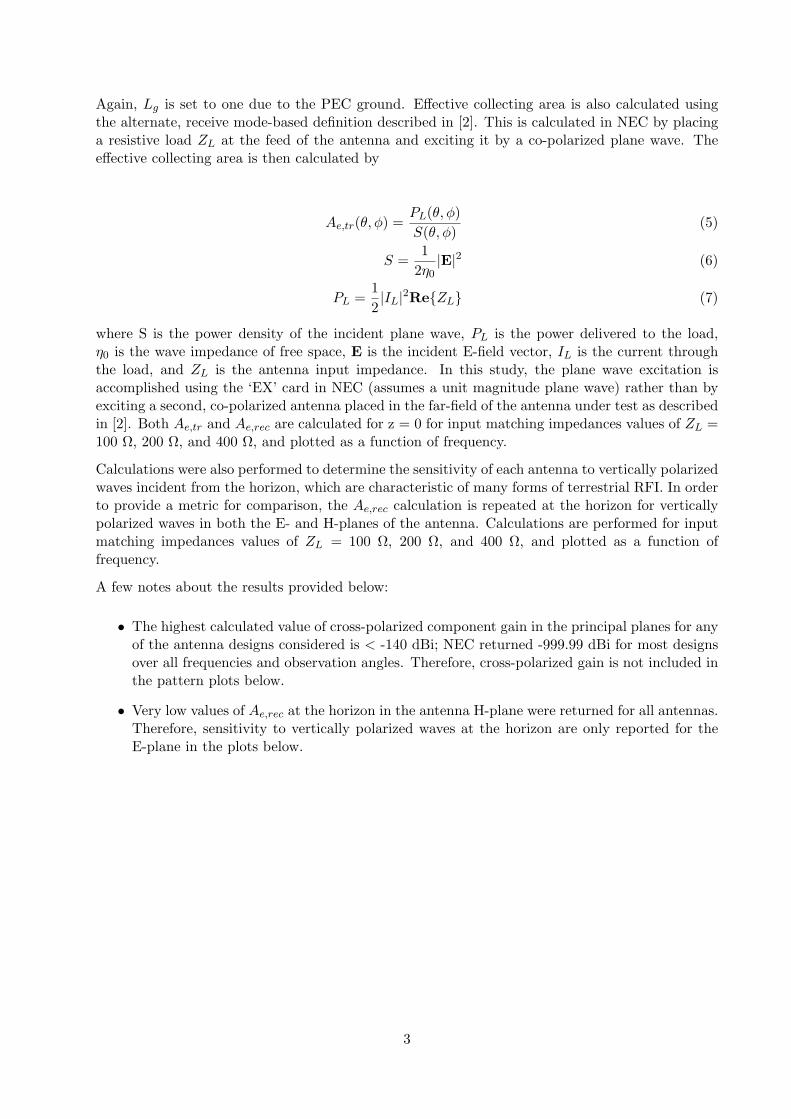
Again, Lg is set to one due to the PEC ground. Effective collecting area is also calculated usingthe alternate, receive mode-based definition described in [2]. This is calculated in NEC by placinga resistive load ZL at the feed of the antenna and exciting it by a co-polarized plane wave. Theeffective collecting area is then calculated by

Ae,tr(θ, φ) =PL(θ, φ)S(θ, φ)

(5)

S =1

2η0|E|2 (6)

PL =12|IL|2ReZL (7)

where S is the power density of the incident plane wave, PL is the power delivered to the load,η0 is the wave impedance of free space, E is the incident E-field vector, IL is the current throughthe load, and ZL is the antenna input impedance. In this study, the plane wave excitation isaccomplished using the ‘EX’ card in NEC (assumes a unit magnitude plane wave) rather than byexciting a second, co-polarized antenna placed in the far-field of the antenna under test as describedin [2]. Both Ae,tr and Ae,rec are calculated for z = 0 for input matching impedances values of ZL =100 Ω, 200 Ω, and 400 Ω, and plotted as a function of frequency.

Calculations were also performed to determine the sensitivity of each antenna to vertically polarizedwaves incident from the horizon, which are characteristic of many forms of terrestrial RFI. In orderto provide a metric for comparison, the Ae,rec calculation is repeated at the horizon for verticallypolarized waves in both the E- and H-planes of the antenna. Calculations are performed for inputmatching impedances values of ZL = 100 Ω, 200 Ω, and 400 Ω, and plotted as a function offrequency.

A few notes about the results provided below:

• The highest calculated value of cross-polarized component gain in the principal planes for anyof the antenna designs considered is < -140 dBi; NEC returned -999.99 dBi for most designsover all frequencies and observation angles. Therefore, cross-polarized gain is not included inthe pattern plots below.

• Very low values of Ae,rec at the horizon in the antenna H-plane were returned for all antennas.Therefore, sensitivity to vertically polarized waves at the horizon are only reported for theE-plane in the plots below.

3

3 Thin Wire Inverted-V Dipole

The LOFAR low band antenna, which is designed to operate nominally between 30 to 80 MHz,consists of a crossed pair of thin wire “inverted-V” dipoles as shown in Figure 1. Design informationfor this antenna was not available at the time this study was conducted, and thus, dimensions weresurmised from photos and the operating frequency range. The dimensions of the big blade dipole(see section 6), were used as a starting point. However, in order to make a more fair comparisonbetween the different designs, the length of the wire element (for one arm of dipole), L, was increasedfrom roughly 1.7 m to 1.9 m. This was done so that the electrical length of the wire is roughlyequal to that of the blade, which is approximately Lb + Wb/2 where Lb and Wb are the lengthand width, respectively of the blade element. It was then necessary to slightly increase the heightof the wire dipole above the ground, H, to 1.6 m so that the elements were not too close to theground. The droop angle, α, was set to 45 , and the feed gap, wf was set to 0.1 m as in the bigblade. Since the actual thickness of the wire used in the LOFAR low band antennas is unknown,it was assumed to be relatively thin, with a radius rw = 1.5 mm.

The NEC model used to simulate the inverted-V dipole is shown in 2. The calculated metrics forthe thin wire inverted-V dipole are provided in Figures 3-11 and Tables 1-3 in the remainder of thissection.

Figure 1: The LOFAR low band antenna [3].

When paired with a lower input impedance value such as 100 Ω, the thin wire inverted-V dipoleexhibits a relatively narrow-band response. However, a higher bandwidth can be achieved with thisantenna by increasing the input impedance. For example, the bandwidth for TANT ≥ 1000 K isincreased from 19.6 MHz wide to 39 MHz wide by increasing ZL from 100 Ω to 400 Ω.

At 38 MHz and below, the radiation patterns of the thin wire inverted-V in both planes exhibita single, wide beamwidth lobe with the maximum towards the zenith. While a null develops atthe horizon in the H-plane, one does not in E-plane, which is an effect of the PEC ground. Athigher frequencies, the H-plane pattern maintains its shape and increases in beamwidth up to 80MHz. By 74 MHz, however, the E-plane pattern develops a sidelobe at the horizon. At 80 MHz

4

Figure 2: The NEC model used for wire dipoles.

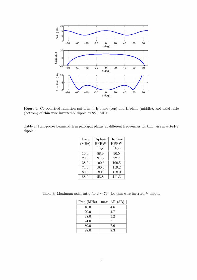
and above, the sidelobe is higher than the mainlobe. Since the difference between the peak andnull is less than 3 dB, high beamwidth is maintained in the E-plane at 74 and 80 MHz accordingthe definition given above. However, a deeper null (4 dB relative to the peak) develops at 88 MHzand the beamwidth is reduced, as can be seen in Table 2. An axial ratio of ≤ 3dB is achieved at allfrequencies < 88 MHz over |z| ≤ 60 . For all frequencies, however, the axial ratio increases rapidlyabove |z| = 60 , and the peak axial ratios reported all occur at |z| = 74 .

As with the sky noise metric, pairing a thin wire inverted-V dipole with a low input impedanceleads to very high values of effective collecting area at the zenith near the half-wave resonance point(near 37.5 MHz in this case), and relatively low values at other frequencies. By increasing ZL, theeffective area at higher and lower frequencies can be increased at the expense of the effective areanear resonance. For instance, by increasing ZL from 100 Ω to 400 Ω, the effective area at zenithis increased by a factor of 3.2 at 74 MHz. For each value of ZL, the transmit and receive-basedcalculations of effective area exhibit similar characteristics at all frequencies, though the transmitbased calculation is up to 4.3 % higher than the receive based calculation.

The thin wire inverted-V dipole is more sensitive to vertically polarized signals at the horizon nearthe half-wave resonance and less sensitive at other frequencies when a low value of input impedanceis used. Sensitivity is increased at higher and lower frequencies by increasing the input impedance.

Table 1: Frequency ranges (in MHz) over which given values of Tant are achieved with thin wireinverted-V dipole for different values of ZL.

TANT > 500 K TANT > 1000 K TANT > 1750 K TANT > 2500 KZL = 100 Ω 26.6 - 56.5 28.9 - 48.5 30.7 - 44.4 31.8 - 42.3ZL = 200 Ω 24.7 - 70.1 27.7 - 55.0 30.2 - 47.9 31.8 - 44.4ZL = 400 Ω 23.3 - 95.8 27.5 - 66.5 31.7 - 53.5 36.1 - 45.6

5

10 20 30 40 50 60 70 80 90 1000

500

1000

1500

2000

2500

3000

3500

4000

Frequency (MHz)

TA

NT (

K)

ZL = 100 Ω

ZL = 200 Ω

ZL = 400 Ω

Figure 3: Sky noise frequency response of thin wire inverted-V dipole for different values of ZL.

−80 −60 −40 −20 0 20 40 60 80−5

0

5

10

z (deg.)

Gai

n (d

Bi)

−80 −60 −40 −20 0 20 40 60 80−10

0

10

z (deg.)

Gai

n (d

Bi)

−80 −60 −40 −20 0 20 40 60 800

5

10

z (deg.)

Axi

al R

atio

(dB

)

Figure 4: Co-polarized radiation patterns in E-plane (top) and H-plane (middle), and axial ratio(bottom) of thin wire inverted-V dipole at 10.0 MHz.

6

−80 −60 −40 −20 0 20 40 60 80−5

0

5

10

z (deg.)G

ain

(dB

i)

−80 −60 −40 −20 0 20 40 60 80−10

0

10

z (deg.)

Gai

n (d

Bi)

−80 −60 −40 −20 0 20 40 60 800

5

10

z (deg.)

Axi

al R

atio

(dB

)


−80 −60 −40 −20 0 20 40 60 80−5

0

5

10

z (deg.)

Gai

n (d

Bi)

−80 −60 −40 −20 0 20 40 60 80−10

0

10

z (deg.)

Gai

n (d

Bi)

−80 −60 −40 −20 0 20 40 60 800

5

10

z (deg.)

Axi

al R

atio

(dB

)


7

−80 −60 −40 −20 0 20 40 60 80−5

0

5

10

z (deg.)G

ain

(dB

i)

−80 −60 −40 −20 0 20 40 60 80−10

0

10

z (deg.)

Gai

n (d

Bi)

−80 −60 −40 −20 0 20 40 60 800

5

10

z (deg.)

Axi

al R

atio

(dB

)


−80 −60 −40 −20 0 20 40 60 80−5

0

5

10

z (deg.)

Gai

n (d

Bi)

−80 −60 −40 −20 0 20 40 60 80−10

0

10

z (deg.)

Gai

n (d

Bi)

−80 −60 −40 −20 0 20 40 60 800

5

10

z (deg.)

Axi

al R

atio

(dB

)


8

−80 −60 −40 −20 0 20 40 60 80−5

0

5

10

z (deg.)

Gai

n (d

Bi)

−80 −60 −40 −20 0 20 40 60 80−10

0

10

z (deg.)

Gai

n (d

Bi)

−80 −60 −40 −20 0 20 40 60 800

5

10

z (deg.)

Axi

al R

atio

(dB

)


Table 2: Half-power beamwidth in principal planes at different frequencies for thin wire inverted-Vdipole.

Freq E-plane H-plane(MHz) HPBW HPBW

(deg) (deg)10.0 88.9 90.520.0 91.3 92.738.0 100.6 100.574.0 180.0 119.280.0 180.0 118.088.0 58.8 111.3

Table 3: Maximum axial ratio for z ≤ 74 for thin wire inverted-V dipole.

Freq (MHz) max. AR (dB)10.0 4.620.0 4.738.0 5.274.0 7.180.0 7.688.0 8.3

9

10 20 30 40 50 60 70 80 90 1000

5

10

15

20

25

Frequency (MHz)

Aef

f (m

2 )

ZL = 100 Ω, tran.

ZL = 200 Ω, tran.

ZL = 400 Ω, tran.

ZL = 100 Ω, rec.

ZL = 200 Ω, rec.

ZL = 400 Ω, rec.

Figure 10: Effective collecting area frequency response at boresight of thin wire inverted-V dipolefor different values of ZL.

10 20 30 40 50 60 70 80 90 1000

1

2

3

4

5

6

7

8

9

10

Frequency (MHz)

Aef

f (m

2 )

ZL = 100 Ω

ZL = 200 Ω

ZL = 400 Ω

Figure 11: Effective collecting area frequency response at horizon of thin wire inverted-V dipole fordifferent values of ZL.

10

4 Thick Wire Inverted-V Dipole

As it is expected that the bandwidth of the inverted-V dipole would increase by increasing theradius of the wire elements, all of the performance metrics were re-calculated assuming the radiusof the wire element was increased to 10.0 mm. This wire radius is intended to simulate a thick wirebraid as used in the fork dipole (see section 7). All other dimensions of the antenna were assumedto be the same as in section 3.

The calculated metrics for the thick wire dipole are provided in Figures 12-20 and Tables 4-6 inthe remainder of this section.

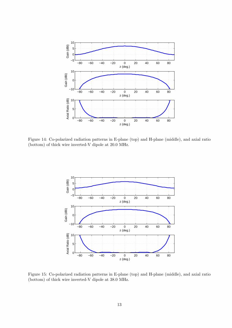
Similar trends with frequency and input impedance are seen in each of the performance metrics forthe thick wire inverted-V as those for the thin wire version. Noted differences between the resultsfor the two antennas are summarized below:

• As expected, the sky noise bandwidth of the thick wire inverted-V is higher than that of thethin wire version. For ZL = 100 Ω, the bandwidth is increased from 19.6 MHz wide for thethin wire dipole to 26.2 MHz wide for the thick wire dipole. For ZL = 400 Ω, the bandwidthis increased from 39 MHz wide to 48.6 MHz wide.

• The height of sidelobes and depths of nulls (up to 5 dB relative to the peak at 88 MHz)are greater for the thick wire dipole than the thin wire dipole. This causes the calculatedbeamwidths to be somewhat lower for the thick wire dipole.

• The maximum axial ratio values are slightly higher at all frequencies for the thick wire dipole.

• The thick wire dipole exhibits somewhat higher values of effective area at the zenith for allfrequencies and all values of input impedance. Interestingly, the receive-based calculation ofeffective area is higher (up to 9.2 %) than the transmit calculation for the thick wire dipole;the opposite was true for the thin wire dipole.

• Sensitivity to vertically polarized signals at the horizon is also higher at all frequencies andvalues of input impedance for the thick wire dipole than the thin wire dipole.

Table 4: Frequency ranges (in MHz) over which given values of Tant are achieved with thick wireinverted-V dipole for different values of ZL.

TANT > 500 K TANT > 1000 K TANT > 1750 K TANT > 2500 KZL = 100 Ω 23.7 - 65.4 26.3 - 52.5 28.4 - 46.6 29.8 - 43.8ZL = 200 Ω 21.8 -100.0 25.1 - 62.7 27.8 - 52.4 29.7 - 47.4ZL = 400 Ω 20.8 - 95.9 25.3 - 73.9 29.9 - 61.3 33.9 - 53.5

11

10 20 30 40 50 60 70 80 90 1000

500

1000

1500

2000

2500

3000

3500

4000

Frequency (MHz)

TA

NT (

K)

ZL = 100 Ω

ZL = 200 Ω

ZL = 400 Ω

Figure 12: Sky noise frequency response of thick wire inverted-V dipole for different values of ZL.

−80 −60 −40 −20 0 20 40 60 80−5

0

5

10

z (deg.)

Gai

n (d

Bi)

−80 −60 −40 −20 0 20 40 60 80−10

0

10

z (deg.)

Gai

n (d

Bi)

−80 −60 −40 −20 0 20 40 60 800

5

10

z (deg.)

Axi

al R

atio

(dB

)

Figure 13: Co-polarized radiation patterns in E-plane (top) and H-plane (middle), and axial ratio(bottom) of thick wire inverted-V dipole at 10.0 MHz.

12

−80 −60 −40 −20 0 20 40 60 80−5

0

5

10

z (deg.)G

ain

(dB

i)

−80 −60 −40 −20 0 20 40 60 80−10

0

10

z (deg.)

Gai

n (d

Bi)

−80 −60 −40 −20 0 20 40 60 800

5

10

z (deg.)

Axi

al R

atio

(dB

)


−80 −60 −40 −20 0 20 40 60 80−5

0

5

10

z (deg.)

Gai

n (d

Bi)

−80 −60 −40 −20 0 20 40 60 80−10

0

10

z (deg.)

Gai

n (d

Bi)

−80 −60 −40 −20 0 20 40 60 800

5

10

z (deg.)

Axi

al R

atio

(dB

)


13

−80 −60 −40 −20 0 20 40 60 80−5

0

5

10

z (deg.)G

ain

(dB

i)

−80 −60 −40 −20 0 20 40 60 80−10

0

10

z (deg.)

Gai

n (d

Bi)

−80 −60 −40 −20 0 20 40 60 800

5

10

z (deg.)

Axi

al R

atio

(dB

)


−80 −60 −40 −20 0 20 40 60 80−5

0

5

10

z (deg.)

Gai

n (d

Bi)

−80 −60 −40 −20 0 20 40 60 80−10

0

10

z (deg.)

Gai

n (d

Bi)

−80 −60 −40 −20 0 20 40 60 800

5

10

z (deg.)

Axi

al R

atio

(dB

)


14

−80 −60 −40 −20 0 20 40 60 80−5

0

5

10

z (deg.)

Gai

n (d

Bi)

−80 −60 −40 −20 0 20 40 60 80−10

0

10

z (deg.)

Gai

n (d

Bi)

−80 −60 −40 −20 0 20 40 60 800

5

10

z (deg.)

Axi

al R

atio

(dB

)


Table 5: Half-power beamwidth in principal planes at different frequencies for thick wire inverted-Vdipole.


(deg) (deg)10.0 89.5 90.620.0 91.9 92.638.0 103.0 100.374.0 180.0 115.680.0 83.0 113.488.0 56.0 105.2

Table 6: Maximum axial ratio for z ≤ 74 for thick wire inverted-V dipole.

Freq (MHz) max. AR (dB)10.0 4.720.0 4.838.0 5.474.0 7.980.0 8.388.0 8.8

15

10 20 30 40 50 60 70 80 90 1000

5

10

15

20

25

Frequency (MHz)

Aef

f (m

2 )

ZL = 100 Ω, tran.

ZL = 200 Ω, tran.

ZL = 400 Ω, tran.

ZL = 100 Ω, rec.

ZL = 200 Ω, rec.

ZL = 400 Ω, rec.

Figure 19: Effective collecting area frequency response at boresight of thick wire inverted-V dipolefor different values of ZL.

10 20 30 40 50 60 70 80 90 1000

1

2

3

4

5

6

7

8

9

10

Frequency (MHz)

Aef

f (m

2 )

ZL = 100 Ω

ZL = 200 Ω

ZL = 400 Ω

Figure 20: Effective collecting area frequency response at horizon of thick wire inverted-V dipolefor different values of ZL.

16

5 MWA-like Dipole

The antenna element design for the MWA LFD array is shown in Figure 21. It consists of a crossedpair of vertically oriented bow-tie dipoles. Design information for this antenna was provided byBrian Corey of Haystack Observatory. As this antenna operates nominally between 80 to 300 MHz,it is necessary to scale up its dimensions in order to compare it with antennas designed for use atLWA frequencies. A common scaling factor of 3.6 was applied to all of the dimensions of the MWAdipole, which provides a good fit to the LWA frequency range. The conductors of the scaled MWAdipole were assumed to be thick wires with a radius of 10 mm. This wire radius is intended tosimulate a thick wire braid as used in the fork dipole (see section 7).

The NEC model used to simulate the scaled MWA dipole is shown in Figure 22. The calculatedmetrics for the scaled MWA dipole are provided in Figures 23-31 and Tables 7-9 in the remainderof this section.

Figure 21: The MWA LFD antenna [4].

Unlike the wire dipoles considered above, the MWA dipole provides wide sky noise bandwidth withlower values of ZL. For instance, TANT ≥ 1000 K is achieved over 20.4 to 72.6 MHz with ZL =100 Ω. By increasing ZL to 200 Ω, which appears to provide the best trade-off for all values ofZL considered, TANT ≥ 1000 K is achieved over 19.8 to 84.6 MHz, which covers the entire LWAband. A “bump” is noted in the sky noise response at roughly 95 MHz, which may be due to aunexpected mode being set up in the antenna.

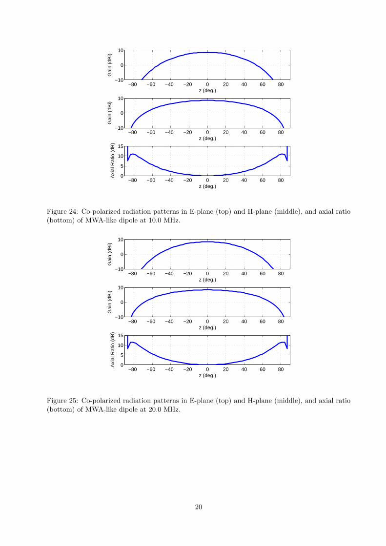
Nulls are exhibited at the horizon in both the E- and H-planes patterns of the MWA dipole, whichis unlike the wire dipoles. However, unlike the nulls in the H-plane which truly go to zero, theE-plane nulls of the MWA dipole are only 10 to 25 dB down from the pattern peaks. The E-plane nulls occur since the arms of the MWA dipole are not bent downward like the other dipole

17

Figure 22: The NEC model used for the MWA-like dipole.

design considered in this report. This aspect of the MWA dipole causes a number of undesirablecharacteristics in its radiation patterns:

• Very low HPBW values are exhibited in E-plane patterns at lower frequencies.

• The pattern shapes in the two principal planes are not well “matched”. This leads to veryhigh maximum axial ratio values, for example 23.9 dB at 74 MHz. Even for |z| ≤ 60 , theaxial ratio is > 5 dB for all frequencies ≤ 38 MHz and > 9 dB for all frequencies ≥ 74 MHz.

• For frequencies ≥ 74 MHz, nulls appear in the patterns at the zenith. Above 74 MHz, nullsare more than 3 dB down from the peak which reduces the pattern beamwidth according tothe definition used in this report.

High values of effective collecting area are achieved at the zenith over a wide frequency range foreach value of ZL. ZL = 200 Ω provides the best trade-off between high values of collecting areaand bandwidth. As with the thick wire dipole, the receive based calculation of collecting area isgreater than the transmit based calculation. Below 90 MHz, the typical difference between the twocalculations is between 6.5 to 8.0 %. However large differences, between 15 to 91 %, are notedbetween 90 to 100 MHz. This behavior is likely to be related to the “bump” noted earlier in thesky noise frequency response.

As compared with other dipole designs considered in this report, the MWA dipole exhibits verylow sensitivity to vertically polarized signals at the horizon over most frequencies. This is due tothe nulls at the horizon, which are evident in the E-plane patterns of the MWA dipole.

18

10 20 30 40 50 60 70 80 90 1000

500

1000

1500

2000

2500

3000

3500

4000

Frequency (MHz)

TA

NT (

K)

ZL = 100 Ω

ZL = 200 Ω

ZL = 400 Ω

Figure 23: Sky noise frequency response of MWA-like dipole for different values of ZL.

Table 7: Frequency ranges (in MHz) over which given values of Tant are achieved with MWA-likedipole for different values of ZL.

TANT > 500 K TANT > 1000 K TANT > 1750 K TANT > 2500 KZL = 100 Ω 17.6 -100.0 20.4 - 72.6 22.9 - 58.3 24.7 - 50.2ZL = 200 Ω 16.1 -100.0 19.8 - 84.6 23.5 - 67.8 26.5 - 58.6ZL = 400 Ω 16.5 -100.0 22.4 - 86.0 29.6 - 73.5 36.6 - 63.5

19

−80 −60 −40 −20 0 20 40 60 80−10

0

10

z (deg.)

Gai

n (d

Bi)

−80 −60 −40 −20 0 20 40 60 80−10

0

10

z (deg.)

Gai

n (d

Bi)

−80 −60 −40 −20 0 20 40 60 800

5

10

15

z (deg.)

Axi

al R

atio

(dB

)

Figure 24: Co-polarized radiation patterns in E-plane (top) and H-plane (middle), and axial ratio(bottom) of MWA-like dipole at 10.0 MHz.

−80 −60 −40 −20 0 20 40 60 80−10

0

10

z (deg.)

Gai

n (d

Bi)

−80 −60 −40 −20 0 20 40 60 80−10

0

10

z (deg.)

Gai

n (d

Bi)

−80 −60 −40 −20 0 20 40 60 800

5

10

15

z (deg.)

Axi

al R

atio

(dB

)


20

−80 −60 −40 −20 0 20 40 60 80−10

0

10

z (deg.)G

ain

(dB

i)

−80 −60 −40 −20 0 20 40 60 80−10

0

10

z (deg.)

Gai

n (d

Bi)

−80 −60 −40 −20 0 20 40 60 800

5

10

15

z (deg.)

Axi

al R

atio

(dB

)


−80 −60 −40 −20 0 20 40 60 80−10

0

10

z (deg.)

Gai

n (d

Bi)

−80 −60 −40 −20 0 20 40 60 80−10

0

10

z (deg.)

Gai

n (d

Bi)

−80 −60 −40 −20 0 20 40 60 800

5

10

15

z (deg.)

Axi

al R

atio

(dB

)


21

−80 −60 −40 −20 0 20 40 60 80−10

0

10

z (deg.)G

ain

(dB

i)

−80 −60 −40 −20 0 20 40 60 80−10

0

10

z (deg.)

Gai

n (d

Bi)

−80 −60 −40 −20 0 20 40 60 800

5

10

15

z (deg.)

Axi

al R

atio

(dB

)


−80 −60 −40 −20 0 20 40 60 80−10

0

10

z (deg.)

Gai

n (d

Bi)

−80 −60 −40 −20 0 20 40 60 80−10

0

10

z (deg.)

Gai

n (d

Bi)

−80 −60 −40 −20 0 20 40 60 800

5

10

15

z (deg.)

Axi

al R

atio

(dB

)


22

Table 8: Half-power beamwidth in principal planes at different frequencies for MWA-like dipole.


(deg) (deg)10.0 66.5 90.520.0 67.5 93.138.0 73.3 104.474.0 101.2 153.480.0 109.2 70.988.0 117.0 52.2

Table 9: Maximum axial ratio for z ≤ 74 for MWA-like dipole.

Freq (MHz) max. AR (dB)10.0 9.620.0 9.938.0 7.874.0 23.980.0 19.388.0 18.5

10 20 30 40 50 60 70 80 90 1000

5

10

15

20

25

Frequency (MHz)

Aef

f (m

2 )

ZL = 100 Ω, tran.

ZL = 200 Ω, tran.

ZL = 400 Ω, tran.

ZL = 100 Ω, rec.

ZL = 200 Ω, rec.

ZL = 400 Ω, rec.

Figure 30: Effective collecting area frequency response at boresight of MWA-like dipole for differentvalues of ZL.

23

10 20 30 40 50 60 70 80 90 1000

1

2

3

4

5

6

7

8

9

10

Frequency (MHz)

Aef

f (m

2 )

ZL = 100 Ω

ZL = 200 Ω

ZL = 400 Ω

Figure 31: Effective collecting area frequency response at horizon of MWA-like dipole for differentvalues of ZL.

24

6 Blade Dipole

The “big blade” dipole, which is a candidate antenna element design for LWA, is shown in Figure32. The dimensions assumed are Lb (length of element) = 1.72 m, Ltap (length of tapered sectionof element) = 0.35 m, β (taper angle of element) = 30 , Wb (width of element) = 0.42 m, α (droopangle) = 45 , H (height of antenna above ground)= 1.52 m, and wf (feed width) = 0.10 m.

The NEC model used to simulate the big blade dipole is shown in Figure 33. The wire radius usedin this model was chosen according to rw = dmesh/(2π) where dmesh is the grid spacing used in themodel. The calculated metrics for the big blade dipole are provided in Figures 34-42 and Tables10-12 in the remainder of this section.

Figure 32: The big blade antenna. Photo obtained from [5].

Figure 33: The NEC model used for the blade dipole.

25

Like the MWA dipole, the blade dipole achieves wide sky noise bandwidth with lower values of ZL.For ZL = 200 Ω, which appears to offer the best performance, TANT ≥ 1000 K is achieved over 20.3to 75.6 MHz. This covers most of the LWA operating band, but is a slightly narrower bandwidththan offered by the MWA dipole for the same value of TANT .

The blade dipole patterns exhibit all the same characteristics and trends with frequency that thewire inverted-V dipoles do. The radiation patterns are sidelobe free for frequencies ≤ 38 MHz, butdevelop sidelobes at 74 MHz and higher frequencies. For frequencies ≥ 80 MHz, the nulls are >3 dB down from the pattern peak, which causes a reduction in the calculated beamwidth. TheHPBW values for the blade dipole are similar to those of the thick wire inverted-V dipole at allfrequencies. The axial ratio values of the blade and thick wire inverted-V dipoles are also similarat all frequencies.

As with the MWA dipole, high values of effective collecting area are achieved at the zenith overa wide frequency range with ZL = 200 Ω giving the best performance. Unlike the thick wireinverted-V dipole and MWA dipoles, the transmit based calculation of effective area is higher thanthe receive based calculation by up to 16.8 %.

The blade exhibits relatively high sensitivity to vertically polarized signals incident from the horizonover a wide frequency range for each of the values of ZL considered.

10 20 30 40 50 60 70 80 90 1000

500

1000

1500

2000

2500

3000

3500

4000

Frequency (MHz)

TA

NT (

K)

ZL = 100 Ω

ZL = 200 Ω

ZL = 400 Ω

Figure 34: Sky noise frequency response of blade dipole for different values of ZL.

Table 10: Frequency ranges (in MHz) over which given values of Tant are achieved with blade dipolefor different values of ZL.

TANT > 500 K TANT > 1000 K TANT > 1750 K TANT > 2500 KZL = 100 Ω 17.4 -100.0 20.3 - 75.6 22.9 - 58.2 24.7 - 51.3ZL = 200 Ω 16.2 -100.0 20.0 - 77.9 23.8 - 65.7 26.8 - 58.7ZL = 400 Ω 17.2 - 86.1 23.3 - 73.8 29.6 - 66.0 34.3 - 61.1

26

−80 −60 −40 −20 0 20 40 60 80−5

0

5

10

z (deg.)

Gai

n (d

Bi)

−80 −60 −40 −20 0 20 40 60 80−10

0

10

z (deg.)

Gai

n (d

Bi)

−80 −60 −40 −20 0 20 40 60 800

5

10

z (deg.)

Axi

al R

atio

(dB

)

Figure 35: Co-polarized radiation patterns in E-plane (top) and H-plane (middle), and axial ratio(bottom) of blade dipole at 10.0 MHz.

−80 −60 −40 −20 0 20 40 60 80−5

0

5

10

z (deg.)

Gai

n (d

Bi)

−80 −60 −40 −20 0 20 40 60 80−10

0

10

z (deg.)

Gai

n (d

Bi)

−80 −60 −40 −20 0 20 40 60 800

5

10

z (deg.)

Axi

al R

atio

(dB

)


27

−80 −60 −40 −20 0 20 40 60 80−5

0

5

10

z (deg.)G

ain

(dB

i)

−80 −60 −40 −20 0 20 40 60 80−10

0

10

z (deg.)

Gai

n (d

Bi)

−80 −60 −40 −20 0 20 40 60 800

5

10

z (deg.)

Axi

al R

atio

(dB

)


−80 −60 −40 −20 0 20 40 60 80−5

0

5

10

z (deg.)

Gai

n (d

Bi)

−80 −60 −40 −20 0 20 40 60 80−10

0

10

z (deg.)

Gai

n (d

Bi)

−80 −60 −40 −20 0 20 40 60 800

5

10

z (deg.)

Axi

al R

atio

(dB

)


28

−80 −60 −40 −20 0 20 40 60 80−5

0

5

10

z (deg.)G

ain

(dB

i)

−80 −60 −40 −20 0 20 40 60 80−10

0

10

z (deg.)

Gai

n (d

Bi)

−80 −60 −40 −20 0 20 40 60 800

5

10

z (deg.)

Axi

al R

atio

(dB

)


−80 −60 −40 −20 0 20 40 60 80−5

0

5

10

z (deg.)

Gai

n (d

Bi)

−80 −60 −40 −20 0 20 40 60 80−10

0

10

z (deg.)

Gai

n (d

Bi)

−80 −60 −40 −20 0 20 40 60 800

5

10

z (deg.)

Axi

al R

atio

(dB

)


29

Table 11: Half-power beamwidth in principal planes at different frequencies for blade dipole.


(deg) (deg)10.0 88.7 90.520.0 91.5 92.538.0 104.9 99.374.0 180.0 110.780.0 79.6 111.988.0 54.8 115.6

Table 12: Maximum axial ratio for z ≤ 74 for blade dipole.

Freq (MHz) max. AR (dB)10.0 4.620.0 4.838.0 5.774.0 8.880.0 8.688.0 7.1

10 20 30 40 50 60 70 80 90 1000

5

10

15

20

25

Frequency (MHz)

Aef

f (m

2 )

ZL = 100 Ω, tran.

ZL = 200 Ω, tran.

ZL = 400 Ω, tran.

ZL = 100 Ω, rec.

ZL = 200 Ω, rec.

ZL = 400 Ω, rec.

Figure 41: Effective collecting area frequency response at boresight of blade dipole for differentvalues of ZL.

30

10 20 30 40 50 60 70 80 90 1000

1

2

3

4

5

6

7

8

9

10

Frequency (MHz)

Aef

f (m

2 )

ZL = 100 Ω

ZL = 200 Ω

ZL = 400 Ω

Figure 42: Effective collecting area frequency response at horizon of blade dipole for different valuesof ZL.

31

7 Fork Dipole

The fork dipole, which is also a candidate antenna element design for LWA was originally discussedin [5] and is shown in Figure 43. All of the dimensions provided in [5] have been assumed herewith the exception that a shorting braid has been added at the bottom of each element in orderto suppress a perturbation in the response near 60 MHz that was exhibited in the original design[6]. As mentioned in [5] a thick wire braid with a radius of approximately 10 mm was used in theoriginal fork design and is assumed here.

The NEC model used to simulate the fork dipole is shown in Figure 44. The calculated metrics forthe fork dipole are provided in Figures 45-53 and Tables 13-15 in the remainder of this section.

Figure 43: The fork antenna (without shorting braid across the bottom of each element). Photoobtained from [5].

While the fork dipole achieves a reasonable bandwidth for which TANT is > 1000K using ZL = 100Ω, the bandwidth is increased significantly to 22.4 to 83.3 MHz using ZL = 200 Ω, which coversmost of the LWA band and is slightly better than the blade dipole for this value of TANT .

Overall, the patterns for the fork dipole are very similar the those of the blade dipole. The nullsbetween the mainlobe and sidelobes at higher frequencies are somewhat reduced for the fork dipoleas compared with the blade dipole (< 3 dB down from peak for frequencies ≤ 80 MHz), however,which improves the calculated beamwidth of the fork dipole at those frequencies. Additionally, themaximum axial ratio for the fork dipole is lower than that of the big blade over all frequencies. Forexample, the improvement at 74 MHz is 29 %.

The frequency response of the effective collecting area at the zenith of the fork dipole is very similarto the blade dipole. Assuming ZL = 200 Ω, the collecting area of the blade dipole is somewhathigher below 67.5 MHz, while that of the fork dipole is higher at higher frequencies. Like the bladedipole, the transmit based calculation of effective area is higher than the receive based calculationfor the fork dipole by up to 14.1 %.

32

Figure 44: The NEC model used for the fork dipole.

While the frequency response of the sensitivity to vertically polarized signals at the horizon issimilar between the two types of antennas, the levels achieved by the fork dipole are lower by afactor of up to nearly two than those of the blade dipole.

10 20 30 40 50 60 70 80 90 1000

500

1000

1500

2000

2500

3000

3500

4000

Frequency (MHz)

TA

NT (

K)

ZL = 100 Ω

ZL = 200 Ω

ZL = 400 Ω

Figure 45: Sky noise frequency response of fork dipole for different values of ZL.

33

Table 13: Frequency ranges (in MHz) over which given values of Tant are achieved with fork dipolefor different values of ZL.

TANT > 500 K TANT > 1000 K TANT > 1750 K TANT > 2500 KZL = 100 Ω 19.9 -100.0 22.8 - 66.6 25.4 - 53.1 27.1 - 47.4ZL = 200 Ω 18.4 -100.0 22.4 - 83.3 26.3 - 63.7 29.6 - 53.8ZL = 400 Ω 19.1 -100.0 25.6 - 85.1 33.5 - 71.8 41.4 - 61.7

−80 −60 −40 −20 0 20 40 60 80−5

0

5

10

z (deg.)

Gai

n (d

Bi)

−80 −60 −40 −20 0 20 40 60 80−10

0

10

z (deg.)

Gai

n (d

Bi)

−80 −60 −40 −20 0 20 40 60 800

5

10

z (deg.)

Axi

al R

atio

(dB

)

Figure 46: Co-polarized radiation patterns in E-plane (top) and H-plane (middle), and axial ratio(bottom) of fork dipole at 10.0 MHz.

34

−80 −60 −40 −20 0 20 40 60 80−5

0

5

10

z (deg.)G

ain

(dB

i)

−80 −60 −40 −20 0 20 40 60 80−10

0

10

z (deg.)

Gai

n (d

Bi)

−80 −60 −40 −20 0 20 40 60 800

5

10

z (deg.)

Axi

al R

atio

(dB

)


−80 −60 −40 −20 0 20 40 60 80−5

0

5

10

z (deg.)

Gai

n (d

Bi)

−80 −60 −40 −20 0 20 40 60 80−10

0

10

z (deg.)

Gai

n (d

Bi)

−80 −60 −40 −20 0 20 40 60 800

5

10

z (deg.)

Axi

al R

atio

(dB

)


35

−80 −60 −40 −20 0 20 40 60 80−5

0

5

10

z (deg.)G

ain

(dB

i)

−80 −60 −40 −20 0 20 40 60 80−10

0

10

z (deg.)

Gai

n (d

Bi)

−80 −60 −40 −20 0 20 40 60 800

5

10

z (deg.)

Axi

al R

atio

(dB

)


−80 −60 −40 −20 0 20 40 60 80−5

0

5

10

z (deg.)

Gai

n (d

Bi)

−80 −60 −40 −20 0 20 40 60 80−10

0

10

z (deg.)

Gai

n (d

Bi)

−80 −60 −40 −20 0 20 40 60 800

5

10

z (deg.)

Axi

al R

atio

(dB

)


36

−80 −60 −40 −20 0 20 40 60 80−5

0

5

10

z (deg.)

Gai

n (d

Bi)

−80 −60 −40 −20 0 20 40 60 80−10

0

10

z (deg.)

Gai

n (d

Bi)

−80 −60 −40 −20 0 20 40 60 800

5

10

z (deg.)

Axi

al R

atio

(dB

)


Table 14: Half-power beamwidth in principal planes at different frequencies for fork dipole.


(deg) (deg)10.0 87.0 90.520.0 88.7 92.238.0 96.4 98.774.0 180.0 116.380.0 180.0 118.388.0 74.6 120.5

Table 15: Maximum axial ratio for z ≤ 74 for fork dipole.

Freq (MHz) max. AR (dB)10.0 4.220.0 4.338.0 4.974.0 6.880.0 6.988.0 6.9

37

10 20 30 40 50 60 70 80 90 1000

5

10

15

20

25

Frequency (MHz)

Aef

f (m

2 )

ZL = 100 Ω, tran.

ZL = 200 Ω, tran.

ZL = 400 Ω, tran.

ZL = 100 Ω, rec.

ZL = 200 Ω, rec.

ZL = 400 Ω, rec.

Figure 52: Effective collecting area frequency response at boresight of fork dipole for different valuesof ZL.

10 20 30 40 50 60 70 80 90 1000

1

2

3

4

5

6

7

8

9

10

Frequency (MHz)

Aef

f (m

2 )

ZL = 100 Ω

ZL = 200 Ω

ZL = 400 Ω

Figure 53: Effective collecting area frequency response at horizon of fork dipole for different valuesof ZL.

38

8 Comparison of Designs

Plots are provided in this section for each metric, which compare the responses of all the antennadesigns considered in this report.

If the pre-amp input impedance is constrained to be a low value such as 100 Ω, the broadbanddipoles considered offer significantly better sky noise bandwidth than do the wire inverted-V dipoles.The blade dipole and MWA dipole sky noise responses are nearly identical having TANT > 1000 Kbetween 20.3 to 75.6 MHz and 20.4 to 72.6 MHz, respectively. The bandwidth of the fork dipoleis slightly reduced with TANT > 1000 K between 22.8 to 66.6 MHz. Even with the thick wireinverted-V dipole, the bandwidth achieved is only 27.5 to 50 MHz.

However, when paired with the optimal value of ZL the results are somewhat different. Thoughthe blade dipole offers higher values of TANT over most the band, the fork and MWA dipoles offerslightly better bandwidths for TANT > 1000 K (19.8 to 84.6 MHz for the MWA dipole, 22.4 to 83.3MHz for the fork dipole, and 20.0 to 77.9 MHz for the blade.) When paired with ZL = 400 Ω, thethick wire dipole achieves TANT > 1000 K over 25.3 to 73.9 MHz, which is a significant portion ofthe LWA band.

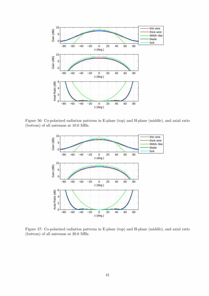
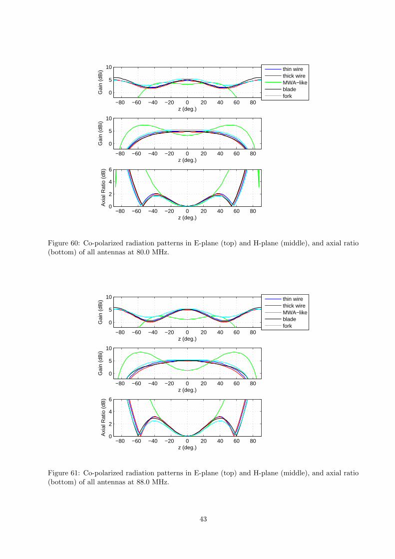
The radiation patterns of the MWA dipole are clearly much different and worse than those ofthe other antennas as discussed in Section 5. The patterns of the remaining antennas exhibitsimilar properties over all frequencies. Particularly at lower frequencies ≤ 38 MHz, it is difficult todiscern any significant differences. For frequencies ≥ 74 MHz, all of the antennas exhibit sidelobes.However, the fork dipole appears to be the best in terms of the ratio of mainlobe to sidelobe levelsand the depth of the null between the mainlobe and sidelobe. The blade appears to be the worst inboth regards. These characteristics cause the calculated beamwidth of the fork to be much higherat 80 MHz than the other antennas. Excepting the MWA dipole, all of the antennas have low axialratio values for |z| ≤ 60 , especially at or below 80 MHz. The fork and thin wire inverted-V dipolesgive the best axial ratio for |z| > 60 for all frequencies. The blade dipole typically exhibits theworst axial ratio for higher zenith angles.

The MWA dipole has the highest effective collecting area at the zenith over all frequencies and forboth values of ZL. This is due to the wideband matching and higher directivity patterns that thisdipole exhibits. Having a higher directivity implies that the collective area at angles away fromthe zenith, however, will be reduced compared to antennas with wider pattern beamwidths. ForZL = 100 Ω, the blade and fork dipoles both provide high collecting area over a wide frequencyrange, though the values of the blade are somewhat higher. The wire dipoles exhibit high peakcollecting area near their half-wave resonance, but very low values at other frequencies. With thebest value of ZL, the blade dipole offers the highest collecting area (besides the MWA antenna)below 60 MHz, while the fork dipole is somewhat better at higher frequencies. The collecting areasof the wire dipoles are still much worse at lower frequencies, though that of the thick wire versionwith ZL = 400 Ω is much more comparable at higher frequencies to the fork and blade dipoles.

For both values of ZL, the blade dipole gives the highest sensitivity to vertically polarized signalsat the horizon over nearly all frequencies. This is due to the higher sidelobes in the blade dipoleradiation patterns, which were noted in Section 6. On the other hand, the MWA dipole exhibitsmuch lower sensitivity than other antennas over nearly all frequencies for both values of ZL due tothe nulls it exhibits at the horizon in the E-plane as discussed in Section 5. With ZL = 100 Ω thewire dipoles exhibit high sensitivity near their half-wave resonance, but much lower sensitivity atother frequencies. The sensitivity of the fork dipole is lower than the blade dipole, but higher thanthe wire dipoles at frequencies away from the wire dipole resonances. When the best value of ZL

is used, the sensitivity of the fork dipole is greater than the thin wire inverted-V dipole, but less

39

than the thick wire version.

10 20 30 40 50 60 70 80 90 1000

500

1000

1500

2000

2500

3000

3500

4000

Frequency (MHz)

TA

NT (

K)

thin wirethick wireMWA−likebladefork

Figure 54: Sky noise frequency response of all antennas for ZL = 100 Ω.

10 20 30 40 50 60 70 80 90 1000

500

1000

1500

2000

2500

3000

3500

4000

Frequency (MHz)

TA

NT (

K)

thin wire, ZL = 400Ω

thick wire, ZL = 400Ω

MWA−like, ZL = 200Ω

blade, ZL = 200Ω

fork, ZL = 200Ω

Figure 55: Sky noise frequency response of all antennas with best value of ZL for each.

40

−80 −60 −40 −20 0 20 40 60 80

0

5

10

z (deg.)G

ain

(dB

i)

−80 −60 −40 −20 0 20 40 60 80

0

5

10

z (deg.)

Gai

n (d

Bi)

−80 −60 −40 −20 0 20 40 60 800

2

4

6

z (deg.)

Axi

al R

atio

(dB

)


Figure 56: Co-polarized radiation patterns in E-plane (top) and H-plane (middle), and axial ratio(bottom) of all antennas at 10.0 MHz.

−80 −60 −40 −20 0 20 40 60 80

0

5

10

z (deg.)

Gai

n (d

Bi)

−80 −60 −40 −20 0 20 40 60 80

0

5

10

z (deg.)

Gai

n (d

Bi)

−80 −60 −40 −20 0 20 40 60 800

2

4

6

z (deg.)

Axi

al R

atio

(dB

)



41

−80 −60 −40 −20 0 20 40 60 80

0

5

10

z (deg.)

Gai

n (d

Bi)

−80 −60 −40 −20 0 20 40 60 80

0

5

10

z (deg.)

Gai

n (d

Bi)

−80 −60 −40 −20 0 20 40 60 800

2

4

6

z (deg.)

Axi

al R

atio

(dB

)



−80 −60 −40 −20 0 20 40 60 80

0

5

10

z (deg.)

Gai

n (d

Bi)

−80 −60 −40 −20 0 20 40 60 80

0

5

10

z (deg.)

Gai

n (d

Bi)

−80 −60 −40 −20 0 20 40 60 800

2

4

6

z (deg.)

Axi

al R

atio

(dB

)



42

−80 −60 −40 −20 0 20 40 60 80

0

5

10

z (deg.)

Gai

n (d

Bi)

−80 −60 −40 −20 0 20 40 60 80

0

5

10

z (deg.)

Gai

n (d

Bi)

−80 −60 −40 −20 0 20 40 60 800

2

4

6

z (deg.)

Axi

al R

atio

(dB

)



−80 −60 −40 −20 0 20 40 60 80

0

5

10

z (deg.)

Gai

n (d

Bi)

−80 −60 −40 −20 0 20 40 60 80

0

5

10

z (deg.)

Gai

n (d

Bi)

−80 −60 −40 −20 0 20 40 60 800

2

4

6

z (deg.)

Axi

al R

atio

(dB

)



43

10 20 30 40 50 60 70 80 90 1000

5

10

15

20

25

Frequency (MHz)

Aef

f (m

2 )


Figure 62: Effective collecting area frequency response at boresight of all antennas for ZL = 100Ω. Note that receive based calculation used.

10 20 30 40 50 60 70 80 90 1000

5

10

15

20

25

Frequency (MHz)

Aef

f (m

2 )




blade, ZL = 200Ω

fork, ZL = 200Ω

Figure 63: Effective collecting area frequency response at boresight of all antennas with best valueof ZL for each. Note that receive based calculation used.

44

10 20 30 40 50 60 70 80 90 1000

1

2

3

4

5

6

7

8

9

10

Frequency (MHz)

Aef

f (m

2 )


Figure 64: Effective collecting area frequency response at horizon of all antennas for ZL = 100 Ω.

10 20 30 40 50 60 70 80 90 1000

1

2

3

4

5

6

7

8

9

10

Frequency (MHz)

Aef

f (m

2 )




blade, ZL = 200Ω

fork, ZL = 200Ω

Figure 65: Effective collecting area frequency response at horizon of all antennas with best valueof ZL for each.

45

9 Conclusions

It should be emphasized that no attempt has been made here to optimize the performance of any ofthe designs considered. Certainly the performance of each design could be improved in terms of atleast one performance metric at a time by changing its design parameters. Additionally, simplifyingassumptions have been made in using an infinite PEC ground and ignoring mutual coupling in thisanalysis. Despite these limitations, it is felt that some basic conclusions can be drawn from theresults presented in this report, and are given below.

• If a 100 Ω active balun input impedance is used, the blade and MWA dipoles provide the bestsky noise bandwidth, while the bandwidth of the fork is somewhat less. The bandwidths ofthe wire inverted-V dipoles considered are much less, and are not suitable given the activebalun noise temperatures being considered for LWA (175 K to 250 K).

• If reasonable active balun noise temperatures can be maintained with higher input impedancevalues, the sky noise bandwidths of the blade and fork dipoles can be improved somewhat,and that of the thick wire inverted-V dipole can be improved significantly to cover a largeportion of the LWA band.

• The radiation patterns of the MWA dipole exhibit very low E-plane beamwidths at low fre-quencies and very high axial ratio values over most frequencies, and therefore are unacceptablefor use in the LWA. The radiation patterns of the remaining antennas are reasonable and ex-hibit similar characteristics over the LWA band. Out of these antennas, the patterns of thefork dipole are somewhat better than the rest, and those of the blade dipole are somewhatworse than the rest in terms of the levels of sidelobes and nulls that appear in the patternsat higher frequencies.

• The fork and blade dipoles offer high values of effective collecting area at the zenith over awide range of frequencies, though the blade dipole values are generally somewhat higher. Ifa low active balun input impedance is used, wire dipoles offer high collecting area only neartheir half-wave resonance frequency. If this impedance can be increased, the collecting areaof the wire dipoles can be increased significantly at other frequencies.

• The blade dipole generally exhibits the highest sensitivity to vertically polarized signals in-cident at the horizon. The relative sensitivity between the fork dipole and the thick wireinverted-V dipole is dependent upon the active balun input impedance used.

Given these conclusions, it is recommended that future antenna studies be focused on blade andfork dipole antennas. If it is possible to achieve reasonable active balun performance with higherinput impedance values (400 Ω or more), then the thick wire dipole should be added to this list.

The simplifying assumptions made in this study should be removed in future studies. For instance,all calculations should be repeated having replaced the infinite PEC ground with a realistic groundscreen in the simulation. This will provide much more realistic radiation pattern calculations andwill include ground loss effects. It is also important to consider the effect of mutual coupling onantenna performance. Mutual coupling between two antennas can be calculated by simulationusing the techniques described in [7]. Additionally, a method for simulating the performance of alarge phased array assuming a particular antenna element design is described in [8]. These methodscould be used to compare the mutual coupling characteristics of different antenna designs.

Although useful for relative comparisons between different antenna designs, the effective collectingarea calculation provided in this report is difficult to relate to the calibratibility requirement for

46

LWA. In future studies, the expression provided in [9] to calculate the number of antenna elementsneeded to calibrate the LWA could be used to compare different candidate designs.

Finally, it was noted that the receive and transmit based calculations of effective collecting areafor a given antenna design generally give different results. The amount of difference between thecalculations varies significantly between designs. Additionally, the calculation that gives the highestvalue of collecting area is not consistent among all designs; that is, the receive calculation does notalways predict a higher collecting area than the transmit calculation, nor vice versa. Further effortshould be spent to better understand these results.

References

[1] H.V. Cane, “Spectra of the Non-Thermal Radio Radiation from the Galactic Polar Regions”,MNRAS, Vol. 189, p. 465, 1979.

[2] S. Ellingson, “Use of NEC-2 to Calculate Collecting Area”, LWA memo No. 65, Dec. 27, 2006.

[3] photo obtained from http://www.lofar.nl/photos .

[4] photo obtained from http://www.haystack.mit.edu/ .

[5] N. Paravastu, B. Hicks, P. Ray, W. Erickson, “A New Candidate Active Antenna Design forthe Long Wavelength Array”, LWA memo No. 88, May 30, 2007.

[6] Psersonal communication with N. Paravastu, July 12, 2007.

[7] A. Kerkhoff, “The Calculation of Mutual Coupling Between Two Antennas and its Applicationto the Reduction of Mutual Coupling Effects in a Pseudo-Random Array”, pending memo.

[8] S. Ellingson, “A Design Study Comparing LWA Station Arrays Consisting of Thin Inverted-VDipoles”, LWA memo No. 75, Jan. 28, 2007.

[9] S. Ellingson, “System Parameters Affecting LWA Calibration (Memo 52 Redux)”, LWA memoNo. 94, July 20, 2007.

47

comparison of dipole antenna designs for the lwa of dipole antenna designs for the lwa aaron kerkho...

Documents