0 1988 Alan R. Liss. Inc. Cytometry 9:291-298 (1988)

Comparison of Frequency Distributions in Flow Cytometry’ Christopher Cox, Jay E. Reeder, Roy D. Robinson, Sarah B. Suppes, and Leon L. Wheeless

Division of Biostatistics (C.C.) and Department of Pathology (J.E.R., R.D.R., S.B.S., L.L.W.), University of Rochester Medical Center, Rochester, New York 14642

Received for publication August 17,1987; accepted February 20, 1988

A number of methods have previously been considered for the statistical comparison of flow cytometric frequency distributions. For two distributions, the foremost of these is the Kolmogorov-Smirnov (K-S) test, which has been criticized as “too sensitive.”

We discuss some alternative methods based on the Poisson distribution. The assumption of Poisson variation within channels allows the use of channel-by-channel confidence in- tervals and chi-square tests. These are simple and more appropriate for discrete data than the K-S test. Graphical displays of these and other techniques are presented. We also at- tempt to set the problem in an appropriate context. We argue that any statistical proce-

dure must rest on a reasonable understanding of the nature of the variability in the system. This understanding takes the form of an ap- propriate probability model, which may be approximate but must provide a reasonably accurate description of the data. Incomplete Understanding of the data can lead to inap- propriate analysis. We discuss the assump- tions that underlie our techniques and consider extensions to more complex situations.

Key terms: Histogram comparison, Kolmo- gorov-Smirnov test, Poisson variation, chi- square test, graphical presentation

Data acquisition in flow cytometry is dependent upon the conversion of continuous biological measurements to discrete values. Accuracy is limited by the resolution available in the analog-to-digital conversion hardware that is being used. This conversion can be considered a primary data reduction step.

Data are obtained in this manner from large numbers of cells (lo4 to lo5) and conveniently presented graphi- cally as histograms or frequency polygons. In order for such frequency distributions to be truly representative, cells must be sampled randomly) so that any given cell has an equal chance of being selected for measurement. The use of frequency distributions for samples of this size allows a fairly complete representation of popula- tions of cells. We define the term population as a collec- tion of cells representing a biological system such as a tissue or organ, At this level of generality, such a popu- lation may include a number of subpopulations of differ- ent cell types. For the purposes of our discussion, however, we assume that the characteristics of this pop- ulation are relatively constant over short periods of time and are representative of the status of the biological system.

In many applications, there is a need to compare fre- quency distributions. Beyond the comparison of control to experimental samples, there is also the need to assess the stability and reproducibility of the measurement process. The use of a standard sample (biological or

synthetic, such as microspheres) is necessary for instru- ment alignment and calibration. Criteria for evaluating instrument performance using such standards may be arbitrary and subjective. A quantitative assessment of difference that is based on an understanding of the mea- surement process is needed. Quality control of the mea- surement process is essential for a particular application of flow cytometric technology to achieve widespread use. Statistical control of flow cytometric experiments re- quires the elimination of measurement bias, and estab- lishment of the precision at which true biological effects can be detected. (The term bias refers to systematic shifts as opposed to random measurement errors.)

Data analysis techniques have been developed with a strong dependence on graphical presentation. In some applications, the difference between two distributions is sufficient to allow easy visualization of differences through overlaid display of histograms. However) it is difficult to describe objectively what criteria are used in such an examination, and no quantitative measure of difference is derived.

~ ~

‘This work was supported by the National Cancer Institute under Grants CA33148 and CA41031.

Address reprint requests to Christopher Cox, Ph.D., University of Rochester Medical Center, Division of Biostatistics, Box 630, 601 Elm- wood Avenue, Rochester, NY 14642.

292 COX ET AL.

In this paper, we consider methods for the quantitative comparison of two frequency distributions. We begin with the Kolmogorov-Smirnov (K-S) test and then con- sider methods based on the Poisson distribution. The statistical tests are illustrated with sample data sets. These methods are likely to find application in the de- tection of effects of sample preparation modifications, determination of independence of two or more cell mark- ers, and assessment of the stability of an instrument over the course of an experiment.

STATISTICAL METHODS The K-S test was applied to flow-cytometry data by

Young (11). It is a standard, nonparametric statistical test that allows a quantitative comparison of two fre- quency distributions. Young, in his original paper, and Finch (4) have cautioned that while the test may detect a difference between two distributions, it should not be accepted blindly as a biological meaningful difference. We wish to discuss the correct use of this procedure by focusing on the underlying assumptions required for its validity. This approach will also allow us to address the question of biological vs. statistical significance.

Three primary assumptions are necessary for any com- parison of two frequency distributions. The first assump- tion is that there are two populations of individuals that we wish to study. Such populations may be somewhat hypothetical but should describe reasonably definite groups of individuals. The practical import of the popu- lation concept is to determine to what group of individ- uals the results of a given study apply (individuals who are like the members of the population).

A second and equally important assumption is that the data are randomly sampled from the parent popula- tion. A closely related notion is the representativeness of the data. This assumption is not valid if a systematic bias or random measurement error is present in the data. Young (11) warns of “artifacts of the stain or the flow methodology.” It is not correct to apply the K-S test or any of the other procedures that we shall discuss when such measurement errors are present. A correct analysis requires that bias or measurement error either be removed experimentally or accounted for in the anal- ysis. More complex statistical models that can estimate the nature of such disturbances and use such estimates to provide the appropriate standard of variability against which to evaluate experimental effects may be required.

A third assumption is that the underlying probability distributions for the two populations are continuous. Use of the K-S test with discrete or binned data is known to be conservative (6). This means that the true P value is really smaller than the value obtained from tables. The consequence is that real effects may be missed. Furthermore, the test is no longer nonparametric; that is, the P value depends on the underlying distribu- tions (7).

As an alternative to the K-S test, we consider methods of comparison that are appropriate for discrete, i.e.

test based on the multinomial distribution. In large sam- ples, however, we may utilize the fact that the distribu- tion of the cell count in a given channel is approximately Poisson (under the simple random sampling assump- tions mentioned earlier, and provided that the relative frequency is not too small). In channels with a reasona- ble number of counts (20 or more), we may use this approximate Poisson behavior to develop channel-by- channel confidence intervals and tests. If n l i and n2i are the counts in channel i from samples of size nl and n2, then the relative frequencies are:

(1)

Using properties of the Poisson distribution, we then have:

z i = ’li - p2i is approximately (2) Pli ~ p2i M k n2l

normally distributed with a mean of zero and variance one. We plot these normal deviates against channel number and note where they exceed the limits of k2. This provides a graphical comparison similar to that of

1 .0 1 0.9

c 0.8 U an u 0 . 1 1 a

0.6--

V

0.5 F r _ _ e 0.4

: i e 0.3

t Theoretical Raw Data Binned Data

- ............. - _ ~

K-S S t a t i s t i c

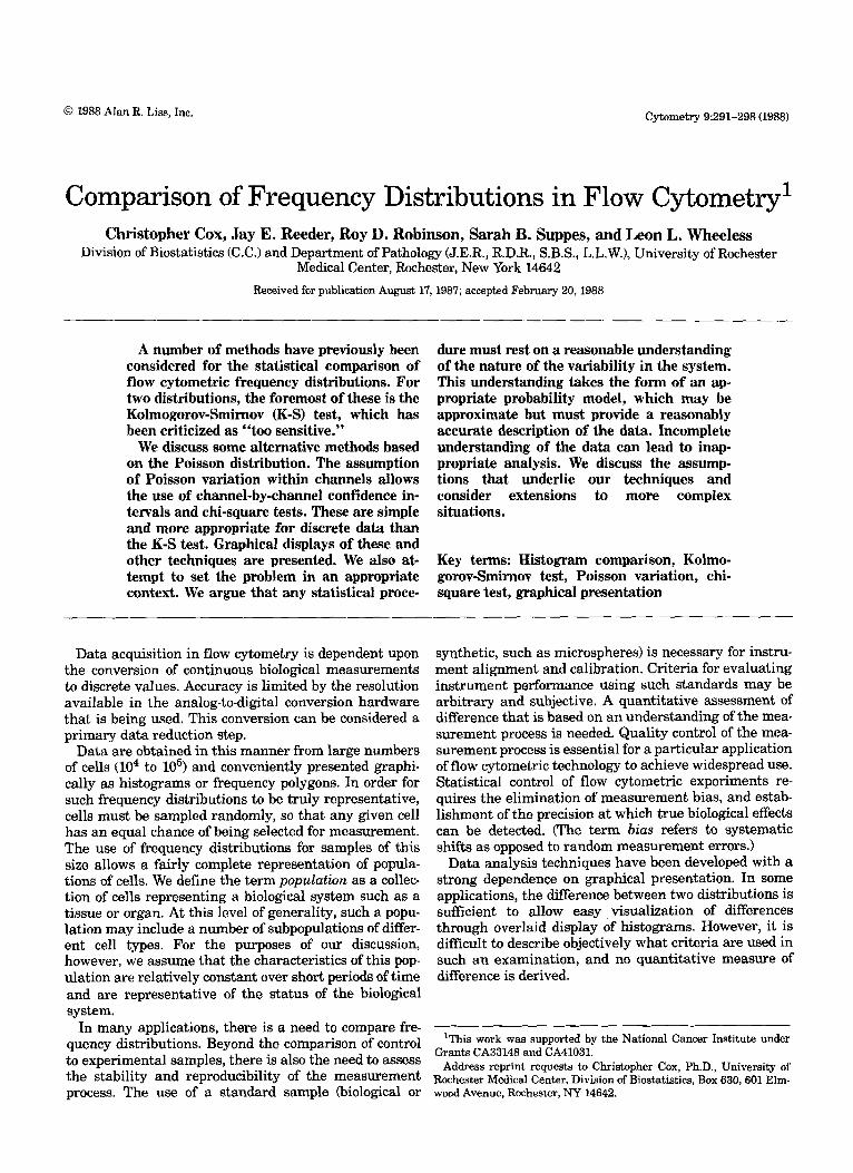
FIG. 1. Cumulative distribution of the Kolmogorov-Smirnov statis- tic. The solid line represents theoretical values. The dotted line repre- sents the distribution of the K-S statistic obtained for 200 sets of two groups of 5,000 normally distributed random numbers with a mean of 127 and a variance of 30. The dashed line illustrates the effect on the distribution of the K-S statistic of binning the data to whole numbers, resulting in approximately 30 bins. P values for the binned distribu- tions are always less than for the theoretical P value. The K-S test is

binned, data. The standard approach is the chi-square therefore conservative for binned data.

HISTOGRAM COMPARISON 293

1

4 0 60 8 0 100 120 20 0 . 0 0 2

I

0.08

0.07"

1 a

0.06"

V e

0.05 r e 4 0 . 0 4

e n

Y

U

0.03

0 . 0 2

0.01

-0.002 1 t i

- ........ Distribution 1

Distribution 2

-0.008 t

0.101 'A ' ' ' '

0.06

0 . 0 4

; 0.02

Y - , I 1 , - - I - . . - - : ; : , 0 . 0 0

' ' ' ' '

2 30 35 40 4 5 50 55 60 6 5 7 0 7 5 80 8 5

channel C

DistributiDn 1 DiBtKlbUtIOn 2

- .............

FIG. 2. Data are a result of SSFCM analysis of two aliquots of a human bladder irrigation and represent nuclear size. A Relative fre- quency distributions. The modal channel for both aliquots is 32. Distri- bution 1 has 15,091 cells, and distribution 2 has 15,279 cells. B: Cumulative frequencies and difference. The value of the K-S statistic is 0.71 (P = 0.69). C: Rebinned relative frequency distributions and

1.0 C U m u 0.8

a t

0 . 6

e

0 . 4

e ¶

c 0.2 n

Y

U

0.0

0.000

-0.002 D 1

- - -0 .004 ; f f

e - 0 . 0 0 6 n c

e

-0.008

I 1 J 0.000

- 0 . 0 0 4 ;

I ' -0.010

B Channel

Distribution 1 Distribution 2

- .............

0.2 0 . 4 0.6 0.8 1.0 U . 0

O D Ordered P-value -

P-Value Line of identity

.............

normal deviates. A minimum of 20 events is required for the chi- square and normal deviate analyses. The data are grouped to achieve this value. Normal deviate values greater than 2 or less than -2 are considered significant. D: Probability plot of P values for channel-by- channel chi-square values. Deviations from the line of identity indicate differences between the two samples,

294 COX ET AL.

0.01-

Y - 0.00

50 100 150 200 250 0.000

Channel

........... Distribution 1 Distribution 2

-

. . . . ................. . . . . . . . . . t

,i I 50 100 150 200 25

0.071

t 1 1

- 3

C Channel

............ Distribution 1 Distribution 2

-

1.0

n u 0.8

a t

0 . 6

e

0 . 4

e 9

e 0.2 n

Y

U

c

0.0

Channel

Distribution 1 Distribution 2

- .............

N 0 r m a 1

0

1 ; a

2 e t

C

0,005

0.000 I

I 1 B

' -0.005

- ............. p-value

Line of IdentIty

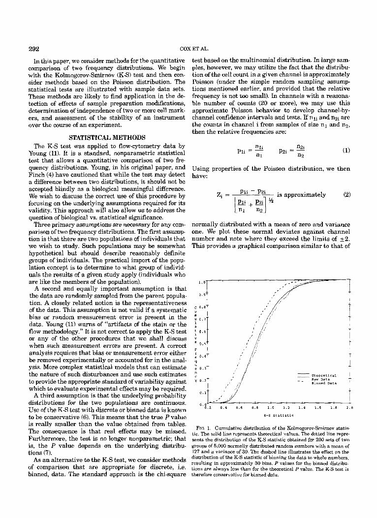
9,530 cells, and distribution 2 has 9,511 cells. B: Cumulative frequen- FIG. 3. Data are a result of SSFCM analysis of two aliquots of a human bladder irrigation and represent cellular DNA stained with propidium iodide. A. Relative frequency distributions. The modal chan- nel of distribution 1 is 48, and 47 for distribution 2. Distribution 1 has

'

cies and difference. The value of the K-S statistic is 2.25 (P < 0.0001). C: Rebinned relative frequency distributions and normal deviates. D: Probability plot of P-values for channel-by-channel chi-square values,

295 HISTOGRAM COMPARISON

Bagwell et al. (1). An overall test of significance may be obtained by squaring and summing the normal deviates to obtain an approximate chi-square statistic with de- grees-of-freedom (df) equal to the number of channels summed.

Further insight into the difference between the two histograms may be obtained by making a probability plot of the P values (9) from the single degree-of-freedom chi-square values obtained by squaring the individual normal deviates, Zi. This is basically a plot of the collec- tion of P values against what would be expected if there were no difference between the two distributions. We sort the P values and plot each one against its rank (as a fraction of the number of P values). If the two histo- grams represent the same population, then the P values will be randomly distributed over the interval from 0 to 1, and the plotted points should follow the line of identity.

The P-value plot provides an indication of the nature of the differences between two frequency distributions. One possible pattern is of a small number of channels where the difference between the two counts is large. This would result in a small number of unusually low P values. Another possibility is that there are a substan- tial number of channels, each with a moderate differ- ence. Either of these situations would contribute t o the magnitude of the overall chi-square statistic. The ap- pearance of the two P-value plots would be different, however. In practice, one would expect differences to occur over ranges of contiguous channels and to be in the same direction. A channel-by-channel plot of the data and P values is useful in examining such questions. An overall significance test is provided by the summary chi-square. It is possible to construct other significance tests based on the probability plot. One could, for exam- ple, perform a K-S test on the P values or some transfor- mation of them. Any such test, however, will be less sensitive than the overall chi-square test, which is de- signed specifically to detect differences between fre- quency counts within channels.

RESULTS A Monte Carlo study was performed to illustrate the

effect of binning the data on the P value of the K-S test. A total of 200 pairs of samples were generated using a computer-based random-number generator. The popula- tion distribution was the same for each pair of samples so that the null hypothesis of the K-S test would be true. The distribution was normal with a mean of 127 and variance 30 (S.D. = 5.48). Samples of 5,000 were gener- ated, and data were then binned to integer values. Thus, the entire sample is included in a range of 33 channels (+3 S.D.). Figure 1 displays a plot of the theoretical cumulative distribution of the K-S statistic together with the observed distribution obtained from the 200 simu- lated values. This agrees quite well with the population distribution. When the data are binned to the nearest integer, however, the resulting cumulative distribution curve moves to the left. The result is that the true P value of the test is much smaller than that given by the population distribution.

To illustrate the two statistical tests, we consider three different examples; the first consists of nuclear size data as measured on a slit-scan flow cytometer (SSFCM) (3,8,10) for two replicate aliquots of a human bladder irrigation sample, stained with propidium iodide. The two histograms are plotted in Figure 2A and are practi- cally identical except for a small shift at the mode and some unevenness in the right tail. The corresponding cumulative distributions are plotted in the first panel of Figure 2B and are indistinguishable. For this reason, we also plot the channel-by-channel differences from these curves, which we call the K-S plot, in the second panel of the figure. The maximum absolute difference is the value on which the K-S test is based. The plot re- veals that the maximum occurs near the modes of the two distributions (channel number 29). The value of the K-S statistic i s 0.71. This was obtained by dividing the maximum differences between the two cumulative fre- quency distributions by a scaling factor that depends on the two sample sizes (11). The P value is 0.69 as is indicated by the theoretical distribution in Figure 1. Thus, the two distributions are not different by this test.

Figure 2C shows the same data rebinned to have at least 20 counts in each channel. There is, of course, a certain amount of arbitrariness in any data-grouping procedure. For samples as large as those we consider, very little rebinning of this sort is typically necessary. The different appearance of Figure 2C illustrates the effect of g-rouping on the appearance of the histograms. The channel-by-channel normal deviates are plotted as error bars below the histograms. Values below -2 (- 1.96) or above +2 (1.96) indicate a statistically signif- icant difference at the 5% level for an individual chan- nel. We see only one such interval and no pattern in the occurrence of positive and negative differences. The overall chi-square statistic summarizing differences across all channels is 37.4 with 32 degrees-of-freedom (the number of bins after regrouping the data). The P value is 0.235, indicating no statistical difference be- tween the two distributions.

The P-value plot is shown in Figure 2D. As one would expect, the observed and expected distributions for the collection of P values agree closely, and the curve (solid) closely follows the line of identity (dotted).

Our second example consists of total (integrated) red fluorescence for two aliquots of a human bladder irriga- tion stained with propidium iodide and analyzed on the SSFCM. The two histograms are presented in Figure 3A. Some discrepancies, including a slight shift in the main peak, are evident.

The two cumulative distributions are difficult to dis- tinguish, but the K-S plot of the channel-by-channel differences shows a large deviation near channel 50, which is close to the modes of the two distributions (Fig. 3B). This difference is due to the shifi noted in Figure 3A. The value of the K-S statistic is 2.25 (P < 0.0001). We conclude that the shift, although slight, is statisti- cally highly significant by the K-S test.

This shift can also be seen in the plot of the channel- by-channel normal deviates (Fig. 3C). The two clusters

COX ET AL. 296

9 U 0.025

n c 0,020 Y

e

0.015

0.010

0.005

50 100 150 200 2 5 0 0.000' x channel

- Distribution 1 Distribution 2

..........

0 . 0 7 7

F + r 0 . 0 3 1 1

1

1 chacnel

............ Distribution 1 Distribution 2

C -

C U m

' -0.03 50 100 150 200 2 5 0

i y '0.02

1 ' - 0 . 0 3

Channel B

- ............. Distribution 1 Distribution 2

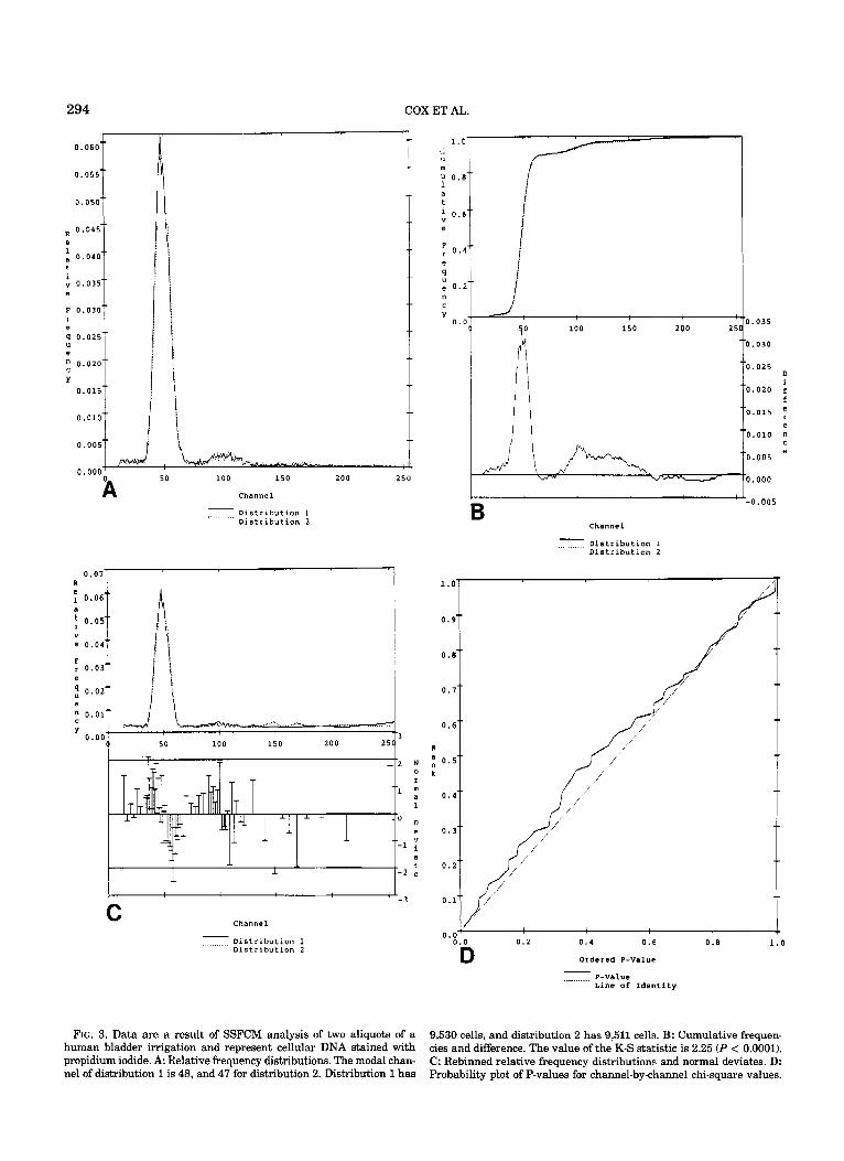
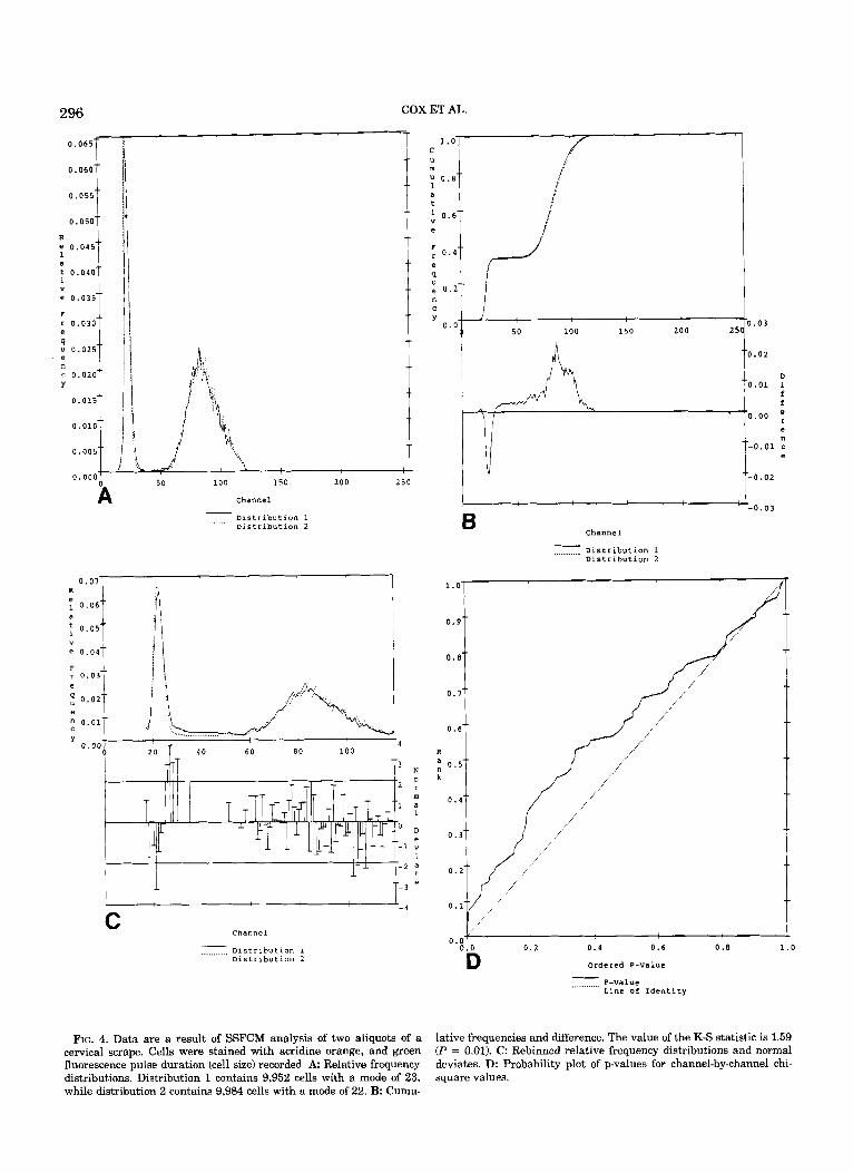
FIG. 4. Data are a result of SSFCM analysis of two aliquot8 of a cervical scrape. Cells were stained with acridine orange, and green fluorescence pulse duration (cell size) recorded A Relative frequency distributions. Distribution 1 contains 9,952 cells with a mode of 23, while distribution 2 contains 9,984 cells with a mode of 22. B: Cumu-

N 0

' r m a 1

' D e

-1 v

- 2 a t

~3

~4

0 . 2 0.4 0.6 0 . e 1.0

Ordered P-value

- P-value ............ Line of Identity

O D

lative frequencies and difference. The value of the K-S statistic is 1.59 (P = 0.01). C: Rebinned relative frequency distributions and normal deviates. D: Probability plot of p-values for channel-by-channel chi- square values.

HISTOGRAM COMPARISON 297

of intervals (one positive, one negative) clearly show the shift. A third possible cluster is seen to the right of these two, suggesting that the left-shifted distribution is catching up. The remaining large deviates reflect zigzag behavior in the right tails. The overall chi-square statis- tic for the grouped data is 80.69 with 73 df (P = 0.25). Thus, no significant difference is indicated.

The P-value plot (Fig. 3D) also indicates the similarity of the two distributions. Thus, we have an indication that the K-S test is more sensitive than the chi-square test to a uniform shift in the distribution of an entire population. The chi-square test, on the other hand, treats all deviations equally and gives no special emphasis to clusters of intervals occurring as the result of a shift.

Our third example involves two truly bimodal distri- butions. The data were obtained on the SSFCM and represent cell size as determined from the green fluores- cence slit-scan contour for two aliquots of a cervical scrape suspension stained with acridine orange. The histograms are shown in Figure 4A. A slight shift can be seen in the left peak and perhaps a very small shift with more up-and-down behavior in the right peak.

The cumulative distributions also reveal some shift- ing, and the K-S plot shows deviations in both peaks, with one distribution falling behind and catching up (Fig. 4B). The value of the K-S statistic is 1.59 (P = 0.011, indicating a significant difference between the two distributions.

The normal deviate plot (Fig. 4C) clearly shows the shift in the left peak but shows more erratic behavior in the right peak. The overall chi-square statistic is 138.24 with 75 df (P = 0.0001). As judged by the relative sizes of the P values, the chi-square test is more sensitive than the K-S in this example. This is probably due to the zigzag behavior of the two distributions in the sec- ond peak. In the P-value plot (Fig. 4D), considerable upward deviation from the line of identity is seen, indi- cating too many small P values for the null hypothesis to be accepted.

DISCUSSION We have illustrated two different statistical proce-

dures for comparing pairs of frequency distributions. One of these is the K-S test, which has been used previ- ously in flow cytometry. In contrast to concerns that the test may be overly sensitive, we have noted that it is conservative with binned data (6). The second approach that we have considered is based on the Poisson distri- bution. Under the assumption of Poisson variation within channels, we constructed channel-by-channel normal deviates. These were plotted to indicate regions (groups of channels) where the two distributions are different. Differences are summarized across channels by a chi-square statistic, which is the sum of the squares of the normal deviates. A probability plot of the individ- ual P values from the normal deviates also helps provide a global assessment. Based on a series of three different data sets, the K-S test appears quite sensitive to a uni- form shift in a population of cells. Alternately, the chi-

square test appears more sensitive to the overall amount rather than the particular pattern of the deviations.

We have also argued that the question of sensitivity must be judged in terms of the nature of the variation in the data. The K-S test may indeed appear too sensi- tive in situations where normal variation is in excess of the sampling variability to be expected when drawing a random sample from a single population. We stress that if such variation is present, then its source and magni- tude must be understood if an adequate statistical anal- ysis is to be possible. From a quality control point of view, one should not use any of the statistical procedures that we have discussed to detect differences between distributions unless the test does not indicate a differ- ence between standard samples.

From another point of view, one can ask about the biological interpretation of differences such as we have found. Young (11) and Finch (4) both caution against overinterpreting the results of statistical tests and em- phasize the distinction between biological and statistical significance. Finch uses the term normal variation to refer to %mall perturbations of the underlying distri- bution,” which presumably contain no biological inf‘or- mation. This term, however, suggests that the basic assumptions of the K-S test are violated in such in- stances. We would argue that the problem is not that the statistical test is too sensitive, but that the nature of the %orma1 variation” has not been properly under- stood. If differences declared significant by the K-S test are to be considered as part of normal variation then we are not simply sampling randomly from a single popu- lation. Sources of additional variation include variabil- ity due to specimen preparation and instrument variation. Whatever the source, this additional varia- tion must be incorporated into the statistical analysis in order to provide the appropriate estimate of variation against which to assess potential biological effects.

In order to ensure valid and ultimately meaningful results, the nature of bias and excess variability in the measurements must be understood and assessed (2). In particular, the presence of systematic shifts and other sources of bias in the measurement process need to be dealt with a t the experimental level.

LITERATURE CITED 1. Bagwell CB, Hudson JL, Irvin G L Nonparametric flow cytometry

analysis. J Histochem Cytochem 27:293-296, 1979. 2. Bailar BA: Quality issues in measurement. Int Stat Rev 53:123-

139,1985. 3. Cambier JL, Kay DB, Wheeless LL: A multidimensional slit-scan

flow system. J Histochem Cytochem 27:321-324, 1979. 4. Finch PD: Substantive difference and the analysis of histograms

from very large samples. J Histochem Cytochem 27:800, 1979. 5. McCullagh P, Nelder, JA: Generalized Linear Models. Chapman

and Hall, New York, 1983. 6. Noether GE: A note on the Kolmogorov-Smirnov statistic in the

discrete case. Metrika 7:115-116, 1963. 7. Pettitt AN, Stephens MA: The Kolmogorov-Smirnov goodness-of-

fit statistic with discrete and grouped data. Technometrics 19:205- 210,1977.

8. Robinson RD, Wheeless DM, Wheeless LL, Hespelt SJ: A system

298 COX ET AL.

for acquisition and real-time processing of multidimensional slit- scan flow cytometric data. Cytometry (submitted for publication).

9. Schweider T, Spyotvoll E: Plots of P values to evaluate many tests simultaneously. Biometrika 69:493-502, 1982.

10. Wheeless LL, Kay DB, Cambier JL: Three dimensional slit-scan

flow system. In: Flow Cytometry IV, Laerum OD, Lindmo T, Thu- rud E (eds). Universitetsforlaget, Oslo, 1980, pp 45-48.

11. Young IT: Proof without prejudice: Use of the Kolmogorov-Smirnov test for the analysis of histograms from flow systems and other sources. J Histochem Cytochem 25:935-941, 1977.