Received: 13 June 2021 Accepted: 26 September 2021

DOI: 10.1002/ppj2.20026

O R I G I N A L R E S E A R C H

Comparison of image georeferencing strategies for agriculturalapplications of small unoccupied aircraft systems

N. Ace Pugh1 Kelly R. Thorp2 Emmanuel M. Gonzalez1

Diaa Eldin M. Elshikha3,4 Duke Pauli1

1 School of Plant Sciences, Univ. of

Arizona, Tucson, AZ 85721, USA

2 USDA-ARS, U.S. Arid-Land Agricultural

Research Center, Maricopa, AZ 85138,

USA

3 Biosystems Engineering, Univ. of Arizona,

Tucson, AZ 85721, USA

4 Agricultural Engineering Dept., Faculty of

Agriculture, Mansoura Univ., Al Mansoura,

Egypt

CorrespondenceDuke Pauli, School of Plant Sciences, Univ.

of Arizona, Tucson, AZ 85721, USA.

Email: dukepauli@arizona.edu

Assigned to Associate Editor Daniel

Northrup.

Funding informationCotton Incorporated, Grant/Award Numbers:

#17-642, #18-384; Yuma Center of Excel-

lence Small Grants Program, Grant/Award

Number: #2019-04; University of Arizona,

Grant/Award Number: Start Up Funds

AbstractSmall unoccupied aircraft systems (sUAS) are becoming popular for mapping appli-

cations in agriculture, and photogrammetry software is available for developing

orthorectified imagery and three-dimensional surface models. Ground control points

(GCPs), which are objects or locations with known geographic coordinates, may be

required for accurate image georeferencing. However, few studies have compared

global position equipment among sUAS or investigated the effects of GCP num-

ber or arrangement on georeferencing accuracy. The objectives of this study were

to evaluate numbers and configurations of GCPs for georeferencing sUAS-acquired

images and determine the GCP requirements for sUAS with and without real-time

kinematic (RTK) global positioning equipment. The effects of varying numbers and

configurations of GCPs were investigated on both a 0.40-ha area the size of a typ-

ical plant breeding trial and a 64.7-ha area (i.e., a U.S. quarter section) the size of

a typical agricultural production field. Results demonstrated that four GCPs placed

at the corners of the breeding-scale field resulted in two-dimensional (2D) error of

±3 cm in the absence of RTK, with minimal improvements when including more

GCPs. The orthomosaics from the RTK-equipped sUAS demonstrated improved 2D

accuracy even without the use of GCPs, with a maximum mean error of 0.08 m. Four

GCPs were found to be sufficient to reduce altitudinal (Z) error, with maximum mean

error of only 0.05 and 1.98 m for the RTK and non-RTK flights, respectively, for the

production-scale field. Thus, using four GCPs, RTK-equipped sUAS, or a combina-

tion will result in improved georeferencing for photogrammetry products.

Abbreviations: DEM, digital elevation map; DSM, digital surface map;

GCP, ground control point; GNSS, global navigation satellite system; GPS,

global positioning system; ODM, OpenDroneMap; P4PRO, Phantom 4 Pro;

P4RTK, Phantom 4 RTK; RGB, red-green-blue; RTK, real-time kinematic;

SfM, structure from motion; sUAS, small unoccupied aircraft systems;

UTM, universal transverse mercator.

This is an open access article under the terms of the Creative Commons Attribution License, which permits use, distribution and reproduction in any medium, provided the original

work is properly cited.

© 2021 The Authors. The Plant Phenome Journal published by Wiley Periodicals LLC on behalf of American Society of Agronomy and Crop Science Society of America

1 INTRODUCTION

Remote sensing technologies are useful for agricultural

research scientists to map their experimental trials (Ander-

son et al., 2019; Araus & Cairns, 2014; Gracia-Romero

et al., 2019; Pauli, Andrade-Sanchez et al., 2016; Shi et al.,

2016). Small unoccupied aircraft systems (sUAS) are a novel

The Plant Phenome J. 2021;4:e20026. wileyonlinelibrary.com/journal/ppj2 1 of 19https://doi.org/10.1002/ppj2.20026

2 of 19 PUGH ET AL.

technology for high-throughput plant phenotyping, which is

the fast and accurate measurement of plant morphology and

properties (Li et al., 2020; Malambo et al., 2018; Pauli, Chap-

man et al., 2016; Sankaran et al., 2015; Singh et al., 2019;

Xie & Yang, 2020). Small unoccupied aircraft system plat-

forms have been used in numerous agricultural studies, imple-

mented in plant breeding programs, and applied in a multitude

of economically important crops worldwide including maize

(Zea mays L.), sorghum [Sorghum bicolor (L.) Moench], cot-

ton (Gossypium hirsutum L.), rice (Oryza sativa L.), and

wheat (Triticum aestivum L.) (Anderson et al., 2019; Gracia-

Romero et al., 2019; Pugh et al., 2018; Yeom et al., 2018;

Zhou et al., 2017). Rotary-wing sUAS, such as quad or hex-

acopters, equipped with red-green-blue (RGB) cameras were

deployed for many of these studies, because they are relatively

simple to use in field-based, agricultural research.

Orthomosaics generated from sUAS-based RGB imagery

can be used to delineate plants or plot boundaries and to

compute vegetation indices. Three-dimensional (3D) struc-

tural details can also be derived from digital surface maps

(DSMs) created using structure from motion (SfM), a process

by which 3D surfaces are reconstructed from a point cloud

created by imaging the scene from multiple angles (Schon-

berger & Frahm, 2016; Westoby et al., 2012). These pho-

togrammetry techniques are important for quantifying pheno-

typic variation in structural plant characteristics, such as plant

height and canopy cover, which are traits that estimate plant

growth and development during a growing season. However,

the geospatial accuracy of photogrammetric products and ulti-

mately plant phenotyping results requires proper georeferenc-

ing of the sUAS image data. The need for high geospatial pre-

cision and accuracy can be addressed using standard tools in

aerial photogrammetry such as ground control points (GCPs)

as well as newer technologies, such as sUAS, that incorporate

real-time kinematic (RTK)-global positioning system (GPS)

equipment (Ekaso et al., 2020; Przybilla et al., 2020). How-

ever, few studies have investigated the use of these techniques

in tandem and for agricultural applications, specifically.

Ground control points are physical objects or locations

for which accurate geographic coordinates are known; they

serve to anchor photogrammetric products to a known, phys-

ical coordinate system (Colomina & Molina, 2014; Rabah

et al., 2018; Westoby et al., 2012). By using GCPs for

which the accurate and precise coordinates are known a pri-

ori, subsequent processing and resulting orthomosaics and

DSMs can be properly georeferenced using a process known

as aerial triangulation (Rabah et al., 2018; Westoby et al.,

2012). This is crucial when the exact spatial relationship

between objects and centimeter-level accuracy is required,

as is frequently the case when image datasets must be

compared with other spatial data sources or when multiple

image sets must be compared over time. This level of accu-

racy is particularly important in studies conducted by plant

Core Ideas∙ Four ground control points are sufficient to georef-

erence aerial photogrammetry projects.

∙ Real-time kinematic positioning data can be used

instead of ground control points (GCPs) to georef-

erence projects.

∙ Using GCPs and real-time kinematic positioning

together results in highly accurate products.

∙ Popular photogrammetry software perform simi-

larly and can each be used for agriculture.

breeders to elucidate specific phenotypes in their chosen crop

or crops; however, many sUAS incorporate GPS that only

achieves meter-level accuracy and may not be suitable for this

purpose (Borra-Serrano et al., 2020; Kawamura et al., 2020;

Su et al., 2019). To obtain centimeter-level accuracy in geo-

referencing scenarios, sUAS must be able to geotag objects

and locations correctly. As noted previously, sUAS equipped

with RTK-GPS technology are becoming an option for sUAS

pilots; however, there has not been rigorous study into their

efficacy when used for plant breeding and agricultural pro-

duction applications.

Although GCPs are simple to implement and efficient to

use, they are nonetheless a primary bottleneck in photogram-

metry processing pipelines (Colomina & Molina, 2014; For-

lani et al., 2019). The choice of GCP material is often dic-

tated by its identifiability in images, how easy they are to

place in the field, and how obstructive they are to field

operations (Forlani et al., 2019). Although it is now widely

understood that multiple GCPs are required to properly geo-

reference imagery collected with sUAS, the number and

configuration of GCPs that are necessary to obtain accu-

rate results is less clear and must also be balanced with

the time required for manual GCP installation and incor-

poration of those GCP data into photogrammetry pipelines

(Villanueva & Blanco, 2019; Wang et al., 2012). Indeed,

the number and placement of GCPs that have been used

by researchers in photogrammetry studies vary widely, even

within the same crop species. For example, in a study con-

ducted in cotton by Thorp et al. (2018), 21 GCPs were iden-

tified from static features around a six-hectare study area,

whereas in another cotton study by Huang et al. (2016), four

GCPs were used to cover each of the 0.6-ha study areas

(Huang et al., 2016; Thorp et al., 2018). Though the usage

of GCPs for georeferencing sUAS imagery is commonplace,

there are few studies that have investigated the effects of GCP

number and configuration on the georeferencing accuracy of

photogrammetry products, and with respect to agricultural

and plant science research, even fewer (Agüera-Vega et al.,

2017; Martínez-Carricondo et al., 2018; Ren et al., 2020;

PUGH ET AL. 3 of 19

Sanz-Ablanedo et al., 2018; Tonkin & Midgley, 2016; Vil-

lanueva & Blanco, 2019; Zimmerman et al., 2020).

Ground control points have been used for image georef-

erencing for several decades, but sUAS capable of geotag-

ging using RTK-GPS, such as the DJI Phantom 4 RTK, have

only recently become available (Forlani et al., 2019; Taddia

et al., 2019). These RTK-equipped sUAS incorporate a sta-

tionary global navigation satellite system (GNSS) receiver

(i.e., base station), which is used to correct positions measured

with the rover GNSS receiver aboard the sUAS. Because the

precise knowledge of the stationary receiver is incorporated

into the triangulation calculations of the location of the rov-

ing receiver, centimeter-level accuracy can be achieved and

applied to the geotagging of images (Fazeli et al., 2016; For-

lani et al., 2018, 2019; Obanawa et al., 2019). Due to this

high level of geospatial accuracy, RTK-equipped sUAS may

permit collection of image data without the need for GCPs

(Rabah et al., 2018). More studies comparing the efficacy of

sUAS platforms with and without RTK technology are needed

to determine how well RTK technology performs, and the

effect of using RTK in tandem with GCPs is also important to

evaluate.

It is important to consider that sUAS merely assign coor-

dinates to image frames during data collection and the use of

photogrammetry software is required to process those image

frames. It is therefore exceedingly difficult to obtain data that

are useful for phenotyping applications from photogrammet-

ric products that do not use some external method to geo-

reference the images, either via GCPs or RTK positioning.

These photogrammetry programs use geotagged images to

develop sparse point clouds, and dense point clouds are devel-

oped using SfM (Schonberger & Frahm, 2016; Westoby et al.,

2012). From the orthomosaics produced by this processing,

researchers and producers can extract useful phenotypes for

their crop of choice. There are several choices of photogram-

metry software available for these sUAS applications, rang-

ing from free and open-source software to proprietary, com-

mercial software. Although researchers have many potential

options, a detailed comparison of the capabilities of each soft-

ware are necessary to identify differences in georeferenced

orthomosaics arising from choice of software.

The conventional wisdom for many agricultural researchers

has been to use as many GCPs as time and funding allows

to attempt to maximize the potential accuracy of photogram-

metry products; however, few studies have investigated GCP

usage and determined when accuracy thresholds are reached.

In addition, RTK technology has not yet been evaluated for

its use when implementing aerial photogrammetry techniques

in plant breeding programs or in agricultural production. To

address these needs, we sought to determine what the optimal

GCP number and configuration for different field scales is and

whether RTK technology could supplement or even replace

GCPs as a georeferencing method in the future. It was also

crucial that several popular photogrammetry software pro-

grams be evaluated and compared for the accuracy of their

products and ability to use those products to extract potential

phenotypes. To assess the impact of using different GCP con-

figurations and RTK technology and identify the best prac-

tices for georeferencing sUAS imagery of agricultural fields,

as well as the differences in the processed imagery between

three popular photogrammetry applications, the objectives of

this study were (a) to determine the most effective number

and configuration of GCPs for aerial photogrammetry from

sUAS, (b) to determine the effectiveness of RTK-equipped

sUAS platforms when compared with non-RTK sUAS, and

(c) to compare the georeferencing accuracy of current pho-

togrammetry software.

2 MATERIALS AND METHODS

2.1 Field site

The experiment used two field areas located at the Mari-

copa Agricultural Center in Maricopa, AZ. The first field

area was 0.4-ha, centered on the coordinates of 408242.279,

3661040.007 (WGS84/universal transverse mercator [UTM]

Zone 12N) and representative of typical plant breeding tri-

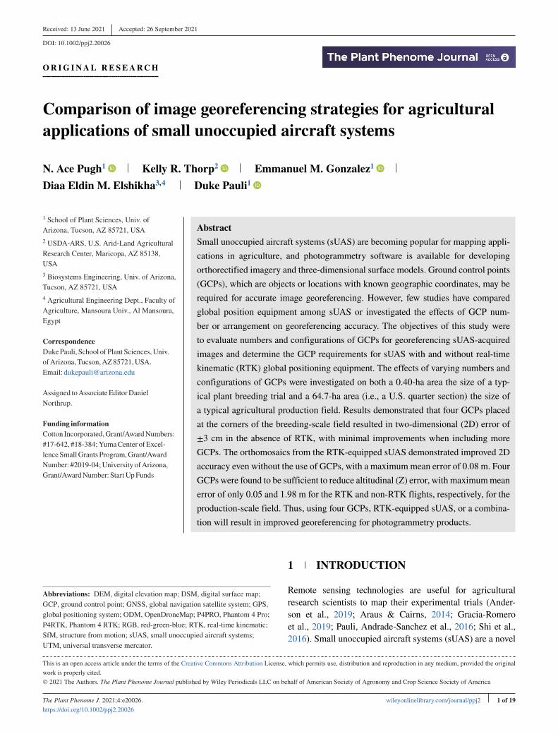
als (“breeding-scale field”, Figure 1a). A total of 63 ground

control points (GCPs) were arranged in a staggered grid pat-

tern with nine rows consisting of seven GCPs with each

row offset from the adjacent row(s) (Figure 1a). The spac-

ing between GCPs from east to west and from north to

south was approximately 7.6 m, and each alternating row

had an offset of approximately 3.8 m. The second field area

was 64.7-ha, a U.S. quarter-section, centered on the coordi-

nates of 408388.680, 3661075.562 (WGS84/UTM Zone 12N)

and representative of a production-scale agricultural field

(“production-scale field,” Figure 1b). A total of 25 GCPs were

placed in a grid pattern with five rows and five GCPs in each

row. The spacing between GCPs from east to west was approx-

imately 188 m, while the spacing from north to south was

approximately 196 m. Preliminary coordinate locations of the

25 GCPs were identified using a digital orthophoto quadran-

gle of the field area, and an RTK-enabled rover was used to

navigate the field area for GCP placement. The breeding-scale

field area was located within the boundaries of the production-

scale field area, but the two field areas did not share any GCPs

in common. Both fields were fallow throughout the entire

study, and a chisel plow had been used to eliminate weeds

prior to the collection of imagery.

White plastic bucket lids (Uline Inc.) with a diameter of

31 cm were used as the GCPs in both field areas, secured

by 30.5-cm metal stakes. To aid in subsequent GCP identi-

fication in photogrammetric software, black crosshairs were

spray painted on each of the GCPs using a stencil, and they

4 of 19 PUGH ET AL.

F I G U R E 1 Field areas and ground control point (GCP)

placement. Layout of GCPs in the 0.4-ha, breeding-scale field area (a)

and the 64.7-ha production-scale field area (i.e., a U.S. quarter section)

(b). Black markers represent the location of each GCP with numbers

representing the GCP identifier

were labeled with an industrial black marker before being

placed in their respective positions. The range of numbers

marked on the GCPs were 65–127 for the breeding-scale field,

and 149–173 for the production-scale field (Figure 1). After

placing all the GCPs in both field areas, geographic coordi-

nates (WGS84/UTM Zone 12N) were measured at the center

of each GCP using an RTK-GPS instrument (Model #5800,

Trimble Inc.).

2.2 Flight planning and image acquisition

Flight missions were conducted over the field areas using a

DJI Phantom 4 RTK (P4RTK; DJI) and a DJI Phantom 4 Pro

v.2 (P4PRO; DJI) (Table 1). For the flights conducted with

the P4PRO, Pix4Dcapture software (Pix4D, Version 4.12.1)

installed on an Apple iPad Mini 4 (Model #MK9P2LL/A;

Apple,) was used to conduct the flight missions. The P4RTK

flights used the onboard mission control software as provided

with the sUAS, and two configurations were tested: with RTK

GPS activated (RTK enabled) and with RTK GPS deacti-

vated (RTK disabled). The initial flights of the breeding-scale

field and the production-scale field were conducted from 16

Oct. to 18 Nov. 2019 (Table 1). An additional set of flights

of the breeding-scale field were also performed on 19 Jan.

2020 to provide a validation dataset using the P4RTK with

RTK enabled and RTK disabled (Table 1). All flights of the

breeding-scale field using both sUAS platforms were con-

ducted at six different altitudes above ground level (AGL): 25,

40, 60, 80, 100, and 120 m. An AGL of 25 m was the lowest

flight altitude permitted by the P4RTK flight control software,

and 120 m AGL was the maximum flight altitude permitted by

U.S. Federal Aviation Administration (FAA) regulations. To

ensure that photogrammetry software could accurately pro-

cess the images, the front and side image overlap was set at

80%. For the production-scale field, flights were conducted

with the P4PRO and the P4RTK with RTK enabled at alti-

tudes of 80, 100, and 120 m AGL, with side and front image

overlaps set at 80%. Flights were conducted during an oper-

ational window spanning 3 h before and after solar noon on

cloud-free days to minimize solar zenith angle, maximize illu-

mination, and minimize shadowing.

2.3 GCP configurations

A variety of GCP configurations were tested during image

processing to identify the optimum number and placement

of GCPs for each field area. The configurations and numbers

of GCPs that were chosen for this study were based on sev-

eral potential scenarios and were an attempt to capture the

minimum level of effective GCP coverage and the threshold

at which improvement in accuracy ceased. Several scenarios

were tested, including placing many GCPs in each area to sim-

ulate heavy GCP coverage, various configurations of four or

five GCPs, one GCP in the center or corner of the field, and

zero GCPs. The purpose of placing zero GCPs was to deter-

mine how effective RTK technology was for georeferencing

alone, and the purpose of placing one GCP was to determine

if the product gained any benefit from the inclusion of a single

GCP or if it was ineffective or detrimental for georeferencing

imagery. In total, eight GCP configurations were tested for the

breeding-scale field: (a) no GCPs; (b) one GCP placed in the

southwest corner of the field (GCP 65); (c) one GCP placed

in the center of the field (96); (d) four GCPs placed at the cor-

ners of the field (65, 71, 121, and 127); (e) four GCPs placed

at the corners and one placed at the center (65, 71, 121, 127,

and 96); (f) four GCPs placed in a box shape nearer to the cen-

ter of the field (89, 90, 103, and 104); (g) nine GCPs spread

evenly across the trial (65, 68, 71, 93, 96, 99, 121, 124, and

127); and (h) the entire set of 63 GCPs (65–127) (Figure 2).

For the production-scale field, six GCP configurations were

tested: (a) no GCPs; (b) one GCP placed at the southwest

corner of the field (169); (c) one center GCP (161); (d) four

PUGH ET AL. 5 of 19

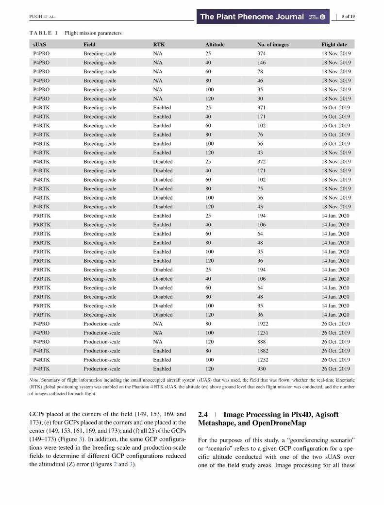
T A B L E 1 Flight mission parameters

sUAS Field RTK Altitude No. of images Flight dateP4PRO Breeding-scale N/A 25 374 18 Nov. 2019

P4PRO Breeding-scale N/A 40 146 18 Nov. 2019

P4PRO Breeding-scale N/A 60 78 18 Nov. 2019

P4PRO Breeding-scale N/A 80 46 18 Nov. 2019

P4PRO Breeding-scale N/A 100 35 18 Nov. 2019

P4PRO Breeding-scale N/A 120 30 18 Nov. 2019

P4RTK Breeding-scale Enabled 25 371 16 Oct. 2019

P4RTK Breeding-scale Enabled 40 171 16 Oct. 2019

P4RTK Breeding-scale Enabled 60 102 16 Oct. 2019

P4RTK Breeding-scale Enabled 80 76 16 Oct. 2019

P4RTK Breeding-scale Enabled 100 56 16 Oct. 2019

P4RTK Breeding-scale Enabled 120 43 18 Nov. 2019

P4RTK Breeding-scale Disabled 25 372 18 Nov. 2019

P4RTK Breeding-scale Disabled 40 171 18 Nov. 2019

P4RTK Breeding-scale Disabled 60 102 18 Nov. 2019

P4RTK Breeding-scale Disabled 80 75 18 Nov. 2019

P4RTK Breeding-scale Disabled 100 56 18 Nov. 2019

P4RTK Breeding-scale Disabled 120 43 18 Nov. 2019

PRRTK Breeding-scale Enabled 25 194 14 Jan. 2020

PRRTK Breeding-scale Enabled 40 106 14 Jan. 2020

PRRTK Breeding-scale Enabled 60 64 14 Jan. 2020

PRRTK Breeding-scale Enabled 80 48 14 Jan. 2020

PRRTK Breeding-scale Enabled 100 35 14 Jan. 2020

PRRTK Breeding-scale Enabled 120 36 14 Jan. 2020

PRRTK Breeding-scale Disabled 25 194 14 Jan. 2020

PRRTK Breeding-scale Disabled 40 106 14 Jan. 2020

PRRTK Breeding-scale Disabled 60 64 14 Jan. 2020

PRRTK Breeding-scale Disabled 80 48 14 Jan. 2020

PRRTK Breeding-scale Disabled 100 35 14 Jan. 2020

PRRTK Breeding-scale Disabled 120 36 14 Jan. 2020

P4PRO Production-scale N/A 80 1922 26 Oct. 2019

P4PRO Production-scale N/A 100 1231 26 Oct. 2019

P4PRO Production-scale N/A 120 888 26 Oct. 2019

P4RTK Production-scale Enabled 80 1882 26 Oct. 2019

P4RTK Production-scale Enabled 100 1252 26 Oct. 2019

P4RTK Production-scale Enabled 120 930 26 Oct. 2019

Note. Summary of flight information including the small unoccupied aircraft system (sUAS) that was used, the field that was flown, whether the real-time kinematic

(RTK) global positioning system was enabled on the Phantom 4 RTK sUAS, the altitude (m) above ground level that each flight mission was conducted, and the number

of images collected for each flight.

GCPs placed at the corners of the field (149, 153, 169, and

173); (e) four GCPs placed at the corners and one placed at the

center (149, 153, 161, 169, and 173); and (f) all 25 of the GCPs

(149–173) (Figure 3). In addition, the same GCP configura-

tions were tested in the breeding-scale and production-scale

fields to determine if different GCP configurations reduced

the altitudinal (Z) error (Figures 2 and 3).

2.4 Image Processing in Pix4D, AgisoftMetashape, and OpenDroneMap

For the purposes of this study, a “georeferencing scenario”

or “scenario” refers to a given GCP configuration for a spe-

cific altitude conducted with one of the two sUAS over

one of the field study areas. Image processing for all these

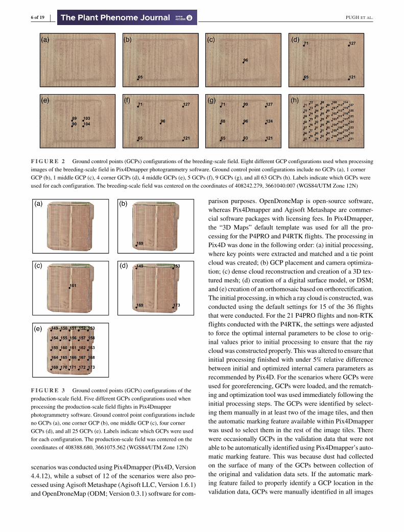
6 of 19 PUGH ET AL.

F I G U R E 2 Ground control points (GCPs) configurations of the breeding-scale field. Eight different GCP configurations used when processing

images of the breeding-scale field in Pix4Dmapper photogrammetry software. Ground control point configurations include no GCPs (a), 1 corner

GCP (b), 1 middle GCP (c), 4 corner GCPs (d), 4 middle GCPs (e), 5 GCPs (f), 9 GCPs (g), and all 63 GCPs (h). Labels indicate which GCPs were

used for each configuration. The breeding-scale field was centered on the coordinates of 408242.279, 3661040.007 (WGS84/UTM Zone 12N)

F I G U R E 3 Ground control points (GCPs) configurations of the

production-scale field. Five different GCPs configurations used when

processing the production-scale field flights in Pix4Dmapper

photogrammetry software. Ground control point configurations include

no GCPs (a), one corner GCP (b), one middle GCP (c), four corner

GCPs (d), and all 25 GCPs (e). Labels indicate which GCPs were used

for each configuration. The production-scale field was centered on the

coordinates of 408388.680, 3661075.562 (WGS84/UTM Zone 12N)

scenarios was conducted using Pix4Dmapper (Pix4D, Version

4.4.12), while a subset of 12 of the scenarios were also pro-

cessed using Agisoft Metashape (Agisoft LLC, Version 1.6.1)

and OpenDroneMap (ODM; Version 0.3.1) software for com-

parison purposes. OpenDroneMap is open-source software,

whereas Pix4Dmapper and Agisoft Metashape are commer-

cial software packages with licensing fees. In Pix4Dmapper,

the “3D Maps” default template was used for all the pro-

cessing for the P4PRO and P4RTK flights. The processing in

Pix4D was done in the following order: (a) initial processing,

where key points were extracted and matched and a tie point

cloud was created; (b) GCP placement and camera optimiza-

tion; (c) dense cloud reconstruction and creation of a 3D tex-

tured mesh; (d) creation of a digital surface model, or DSM;

and (e) creation of an orthomosaic based on orthorectification.

The initial processing, in which a ray cloud is constructed, was

conducted using the default settings for 15 of the 36 flights

that were conducted. For the 21 P4PRO flights and non-RTK

flights conducted with the P4RTK, the settings were adjusted

to force the optimal internal parameters to be close to orig-

inal values prior to initial processing to ensure that the ray

cloud was constructed properly. This was altered to ensure that

initial processing finished with under 5% relative difference

between initial and optimized internal camera parameters as

recommended by Pix4D. For the scenarios where GCPs were

used for georeferencing, GCPs were loaded, and the rematch-

ing and optimization tool was used immediately following the

initial processing steps. The GCPs were identified by select-

ing them manually in at least two of the image tiles, and then

the automatic marking feature available within Pix4Dmapper

was used to select them in the rest of the image tiles. There

were occasionally GCPs in the validation data that were not

able to be automatically identified using Pix4Dmapper’s auto-

matic marking feature. This was because dust had collected

on the surface of many of the GCPs between collection of

the original and validation data sets. If the automatic mark-

ing feature failed to properly identify a GCP location in the

validation data, GCPs were manually identified in all images

PUGH ET AL. 7 of 19

so that consistent use of GCPs was maintained among image

sets. The next stage of processing, where the point cloud and

3D textured mesh were constructed, was performed immedi-

ately after georeferencing was completed. Finally, a DSM and

an orthomosaic were generated that could be used for further

analyses.

After georeferencing in Pix4Dmapper was completed, the

image pixel coordinates of GCP locations in the image tiles,

as during Pix4DMapper processing, were exported from the

software, so identical GCP data could be used for process-

ing with other photogrammetry software. For example, to

georeference images in ODM, a text file (gcplist.txt) was

required to relate the geographic coordinates of the GCPs to

the image coordinates in each of the images that contained a

GCP. Because these data were available from prior process-

ing with Pix4DMapper, the information was reformatted to

the specifications required for ODM. This ensured that the

performance of the software was compared using identical

inputs to relate geographic and image coordinates for each

GCP. OpenDroneMap was run from the command line using

the software’s Docker image (Merkel et al., 2014). Default set-

tings were used except for the “orthophoto-resolution” setting,

which was specified to the resolution of orthomosaic output

from Pix4DMapper to facilitate fair comparisons between the

software. As with the commercial photogrammetry software,

the general workflow in ODM progressed in five steps: (a)

sparse point cloud of ties points using OpenSfM; (b) densi-

fication of the point cloud; (c) meshing to create a 3D sur-

face; (d) texturing using image overlay; and (e) orthophoto

construction.

Processing in Agisoft Metashape was done by following

a similar workflow that was used for Pix4Dmapper. Settings

were chosen to match the default settings used for 3D Maps

in Pix4Dmapper, and similar steps were taken to generate the

resulting orthomosaics. The general workflow in Metashape

progressed in five general steps: (a) tie point cloud construc-

tion, (b) GCP placement and camera optimization, (c) dense

cloud construction, (d) digital elevation map (DEM) construc-

tion, and (e) generation of the orthomosaic. The tie point

cloud, also referred to as the sparse point cloud, was con-

structed by aligning the photos with the key point, and tie

point limits increased from the default levels of 40,000 and

4,000 to 200,000 and 20,000, respectively. Once GCPs were

placed in each scenario, they were identified in at least two

images to ensure the software could automatically identify

their position in all other images in which they occurred. Once

all GCPs were placed into the scenario, cameras were opti-

mized based upon the GCP locations to correct for spatial

error in a similar fashion to the rematching and optimization

process in Pix4Dmapper. To accomplish this, all the cam-

eras were deselected and GCPs were selected before optimiza-

tion was used. To attempt to match the default settings for

the generation of 3D maps in Pix4Dmapper, the dense cloud

was processed at medium quality with aggressive depth fil-

tering. Once the dense point cloud was constructed, a DEM

was constructed using the dense point cloud with interpola-

tion enabled. The orthomosaic was based on the DEM and

was processed using the mosaic blending mode with hole fill-

ing enabled. The DEM and final orthomosaic were both con-

structed using the same UTM projection as the rest of the

georeferencing scenarios in this study (WGS84/UTM Zone

12N). The processing in Pix4Dmapper, ODM, and Agisoft

Metashape was performed using a computer with an Intel

Xeon® CPU E5-2630 v3 (two processors) and 256 GB of

installed RAM.

2.5 Extraction of X, Y, and Z location datausing QGIS software

To extract location data from each orthomosaic and DSM for

the image sets defined in Table 1, the orthomosaics gener-

ated in Pix4Dmapper, Metashape, and ODM were loaded into

QGIS software v.3.8.3 (https://www.qgis.org/ ). To estimate

two-dimensional (2D), horizontal accuracy (i.e., X/Y posi-

tional error), the GCP locations in each orthophoto were iden-

tified, manually marked, and added as a point feature in a new

point layer shapefile. To ensure that point features were placed

consistently, the project zoom was increased until a point that

best approximated the location of the center pixel of each GCP

could be selected. The UTM coordinates of each manually-

selected point were then exported from the attribute table of

the shapefile layer. These UTM coordinates were compared

with the known coordinates measured for each of the GCPs

in the field, as described in the Data Analysis and Statistics

section.

Altitudinal data (Z) were obtained for each GCP using the

DSM generated for each project in Pix4Dmapper. The loca-

tions of the GCPs identified in each of the orthomosaics were

used as the point for which altitude estimates were extracted.

Then, the DSM was placed in the QGIS project, and the alti-

tude estimates were extracted from the DSM using the Point

Sampling Tool plugin. As with the X/Y locations, these esti-

mates of altitude based on the DSM were then compared to

the altitude values that were recorded using the Trimble RTK-

GPS at GCP locations prior to the flight missions.

2.6 Data analysis and statistics

The GCP coordinates from each orthomosaic were exported

from QGIS, and they were associated with the measured GCP

coordinates as recorded by the RTK-GPS prior to the flight

missions. An estimate of two-dimensional horizontal error

was calculated using the following equation (i.e., the dis-

tance formula): d = √([x2 − x1]2 + [y2 − y1]2), where d is

8 of 19 PUGH ET AL.

the estimated two-dimensional error (in meters), x1 is the X

coordinate of the point exported from QGIS, x2 is the mea-

sured X coordinate at the physical center of the GCP in the

field, y1 is the Y coordinate of the point exported from QGIS,

and y2 is the measured Y coordinate the physical center of

the GCP in the field. To estimate Z error, the absolute value

of the difference between the field-measured altitude and the

altitude estimated from the DSM was used.

The means of the error estimates were graphed using the

ggplot2 package in R software (R Development Core Team,

2011; Wickham, 2016). In addition, postplots that showed

the spatial error among GCPs were produced in QGIS for

the breeding-scale field using the flights conducted with the

P4PRO and P4RTK at 60 m altitude AGL and for each GCP

configuration. The same process was used to produce post-

plots for altitudinal error in the production-scale field for

the flights conducted with the P4PRO and P4RTK at 100 m

altitude AGL and for each GCP configuration. To better

visualize differences between these configurations in the

breeding-scale and production-scale postplots, the diameter of

the postplot icons was specified as the computed error +1 m

and error +10 m, respectively.

To assess the consistency of X/Y spatial error estimates

for flights conducted in the fall of 2019 (the original data

set) versus those flights conducted in the early spring of

2020 (the validation data sets) over the breeding-scale field,

two-sided, paired t-tests were carried out using the “t.test”

function in R with a 95% confidence interval (R Development

Core Team, 2011). To carry out the tests, the error estimates

for each individual GCP from the six flight altitudes, GCP

configurations, and RTK settings were treated as paired

data with pairs being “original” and “validation” GCP error

estimates.

Comparisons of software processing time and performance

were carried out using the same above-mentioned worksta-

tion for processing. A subset of georeferencing scenarios

was selected amongst the two drone platforms, with RTK

enabled and disabled, at two flight altitudes (25 and 120 m),

and with four or zero GCPs used for georeferencing. After

completion of the processing for each scenario using each

of the respective software, the total processing time was

recorded and the georeferencing errors associated with indi-

vidual GCPs were compared. Nonparametric Kruskal-Wallis

tests were performed in Python v3.9 using the command

“scipy.kruskal” from the SciPy library to determine if there

were significant differences in the mean georeferencing errors

among the three software (Virtanen et al., 2020). To further

assess differences, nonparametric, pairwise comparisons of

georeferencing errors were performed using Conover tests

(if the Kruskal-Wallis null hypothesis was rejected) using

the “scikit_poshocs.posthoc_conover” from the Scikit library

(Terpilowski, 2019).

3 RESULTS

3.1 Two-dimensional georeferencingaccuracy

The flights conducted at all six altitudes over the breeding-

scale field using the P4PRO exhibited a similar pattern of

decreasing spatial error as the number of GCPs used for geo-

referencing increased from 0 to 63 (Figure 4a). Regardless of

flight altitude, it was clear that forgoing the use of GCPs led to

poor performance with spatial error estimates ranging from a

minimum of 1.48 m for the 40 m altitude up to 2.28 m for the

25 m altitude (Figure 4a). The use of one GCP, either in the

corner or center of the field, resulted in across-altitude mean

error estimates of 0.80 to 0.35 m, respectively. The four cor-

ner, five, and nine GCP configurations all had across-altitude

mean error estimates of 0.03 m while using all 63 GCPs

produced the same spatial mean error estimate of 0.03 m

(Figure 4). The configuration of four middle-of-the-field

GCPs resulted in a slight increase in georeferencing error with

a mean error estimate of 0.04 m. These results demonstrate

that, on average, increasing the number of GCPs used for geo-

referencing to more than four per 0.4-ha study area did not

provide any gain in geospatial accuracy.

For flights conducted using the P4RTK with RTK enabled,

a similar trend was observed as with the P4PRO. Configura-

tions using four or more GCPs resulted in an across-altitude

mean error estimate of 0.03 m while configurations using

only one GCP, either in the corner or the center, resulted in

spatial error accuracies of 0.06 m and 0.05 m, respectively

(Figure 4b). However, the largest difference for geospatial

accuracy when compared with the flights conducted with

P4PRO was observed for the zero GCP configuration; with

RTK enabled, the mean error estimate across altitudes was

0.07 m whereas for the P4PRO it was 1.77 m, a 25-fold

difference in accuracy. Furthermore, the error estimates for

the P4RTK with RTK enabled varied between 0.03–0.08 m

(SD = 0.02 m) among the GCP configurations (including zero

GCPs) compared with a range of 0.02–2.28 m (SD = 0.61 m)

using the P4PRO (Figure 4a, 4b). Not only was the range and

standard deviation of the error estimates for the P4RTK with

RTK enabled much smaller than that observed for the P4PRO,

but the addition of GCPs had less impact on reducing the

georeferencing error as well. The difference in across-altitude

mean error for zero GCPs and four corner GCPs was 0.04 m

for the P4RTK whereas for the P4PRO, that difference was

1.74 m. Thus, the use of GCPs results in an improvement in

georeferencing accuracy but it is less pronounced when using

the Phantom 4 RTK with RTK enabled.

For the P4RTK flights with RTK disabled, the use of four or

more GCPs was effective at improving georeferencing accu-

racy. The across-altitude error estimates were identical to that

PUGH ET AL. 9 of 19

F I G U R E 4 Mean geospatial accuracy. The mean error (m) and standard deviation (m) of the flights conducted for the breeding-scale field with

the Phantom 4 Pro (a), the breeding-scale field with the Phantom 4 real-time kinematic (RTK) with RTK enabled (b), the breeding-scale field with

the Phantom 4 RTK with RTK disabled (c), the production-scale field with the Phantom 4 Pro (d), and the production-scale field with the Phantom 4

RTK with RTK enabled (e). Accuracy was calculated using the Universal Transverse Mercator (UTM) coordinates of each ground control point

(GCP) postprocessing and the coordinates collected for each GCP on the ground using a Trimble RTK global positioning system (RTK-GPS). The

flights were conducted at altitudes of 25, 40, 60, 80, 100, and 120 m AGL for the breeding-scale field and at 80, 100, and 120 m AGL for the

production-scale field. Eight GCP configurations are shown: no GCPs (0), 1 corner GCP (1 C), 1 middle GCP (1 M), 4 corner GCPs (4 C), 4 middle

GCPs (4 M), 5 GCPs, 9 GCPs, and all 63 or 25 GCPs for the breeding-scale and production-scale fields, respectively (63 and 25)

of the P4PRO for four of the GCP configurations; the four cor-

ner, five, and nine GCP configurations resulted in an across-

altitude error estimates of 0.03 m, whereas the configura-

tion with four middle-of-the-field GCPs had an error esti-

mate of 0.04 m (Figure 4c). However, in stark contrast to the

P4PRO and P4RTK with RTK enabled, the accuracy of the

P4RTK with RTK disabled displayed greater errors for the

zero, one corner, and one center GCP configurations; the error

estimates were 1.58, 4.88, and 2.42 m, respectively. As dis-

cussed below, this result is likely related to issues of image

10 of 19 PUGH ET AL.

translation without rescaling that occurs when only one GCP

is used for georeferencing.

Georeferencing accuracy of P4PRO images over the

production-scale field followed similar trends to those

observed with the breeding-scale field; the use of four corner

GCPs achieved nearly the same georeferencing error as using

all 25 GCPs, 0.06 m and 0.04 m, respectively (Figure 4d). In

addition, this level of georeferencing accuracy, 0.04 m, for the

production-scale field using four GCPs was comparable with

that of the breeding-scale field, which had an across altitude

mean error estimate of 0.03 m. Although the error estimates

for four GCPs in the production-scale field was nearly double

that of the breeding-scale, 0.06 m vs. 0.03 m, the study area of

the production field was more than 160 times larger, highlight-

ing the efficacy of GCPs for georeferencing at multiple scales.

Interestingly, the largest georeferencing errors were not found

when GCPs were excluded from the processing but instead

were found when using only one GCP, either in the corner

or in the middle of field, for georeferencing the 120 m alti-

tude flights (Figure 4d). These two configurations produced

across-altitude error estimates of 18.75 m for the one corner

GCP and 16.64 m for the middle-of-the-field GCP layouts,

which were the highest observed spatial 2D error estimates

in the study. The increase in georeferencing error when using

only one GCP, either in the corner or middle of the field, is

likely related to the issue of image translation without neces-

sary rescaling, which is discussed below.

Georeferencing accuracy of the P4RTK images over the

production-scale field was improved compared with the

P4PRO—all configurations had across-altitude error esti-

mates less than 1 m with the highest observed error being

0.08 m (Figure 4e). In addition, the inclusion of four cor-

ner GCPs, the configuration with the lowest georeferencing

error, reduced the spatial error from 0.08 m for zero GCPs to

0.05 m (across altitude mean), a difference of only 3 cm. The

difference in georeferencing accuracy of the P4RTK relative

to the P4PRO was also quite significant for the production-

scale field; the P4PRO had error estimates ranging from 0.04

to 18.75 m (SD = 5.55 m), whereas the P4RTK had values

ranging from 0.04 to 0.08 m (SD = 0.02 m). The use of all

25 GCPs had the lowest georeferencing error estimates with

values of 0.04 m found for all three flight altitudes. As was

obtained for the P4RTK over the breeding-scale field, the dif-

ference in error between using no GCPs and using four was

small; a mean difference of 0.04 m was observed across the

three altitudes flown.

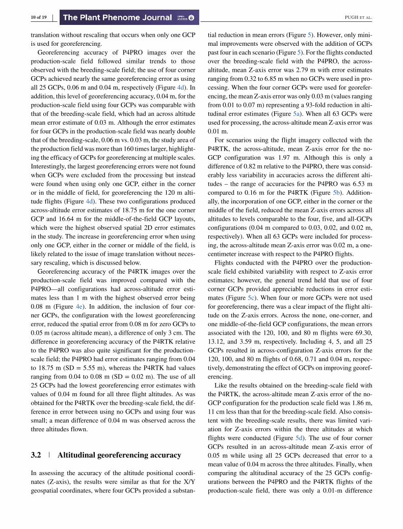
3.2 Altitudinal georeferencing accuracy

In assessing the accuracy of the altitude positional coordi-

nates (Z-axis), the results were similar as that for the X/Y

geospatial coordinates, where four GCPs provided a substan-

tial reduction in mean errors (Figure 5). However, only mini-

mal improvements were observed with the addition of GCPs

past four in each scenario (Figure 5). For the flights conducted

over the breeding-scale field with the P4PRO, the across-

altitude, mean Z-axis error was 2.79 m with error estimates

ranging from 0.32 to 6.85 m when no GCPs were used in pro-

cessing. When the four corner GCPs were used for georefer-

encing, the mean Z-axis error was only 0.03 m (values ranging

from 0.01 to 0.07 m) representing a 93-fold reduction in alti-

tudinal error estimates (Figure 5a). When all 63 GCPs were

used for processing, the across-altitude mean Z-axis error was

0.01 m.

For scenarios using the flight imagery collected with the

P4RTK, the across-altitude, mean Z-axis error for the no-

GCP configuration was 1.97 m. Although this is only a

difference of 0.82 m relative to the P4PRO, there was consid-

erably less variability in accuracies across the different alti-

tudes – the range of accuracies for the P4PRO was 6.53 m

compared to 0.16 m for the P4RTK (Figure 5b). Addition-

ally, the incorporation of one GCP, either in the corner or the

middle of the field, reduced the mean Z-axis errors across all

altitudes to levels comparable to the four, five, and all-GCPs

configurations (0.04 m compared to 0.03, 0.02, and 0.02 m,

respectively). When all 63 GCPs were included for process-

ing, the across-altitude mean Z-axis error was 0.02 m, a one-

centimeter increase with respect to the P4PRO flights.

Flights conducted with the P4PRO over the production-

scale field exhibited variability with respect to Z-axis error

estimates; however, the general trend held that use of four

corner GCPs provided appreciable reductions in error esti-

mates (Figure 5c). When four or more GCPs were not used

for georeferencing, there was a clear impact of the flight alti-

tude on the Z-axis errors. Across the none, one-corner, and

one middle-of-the-field GCP configurations, the mean errors

associated with the 120, 100, and 80 m flights were 69.30,

13.12, and 3.59 m, respectively. Including 4, 5, and all 25

GCPs resulted in across-configuration Z-axis errors for the

120, 100, and 80 m flights of 0.68, 0.71 and 0.04 m, respec-

tively, demonstrating the effect of GCPs on improving georef-

erencing.

Like the results obtained on the breeding-scale field with

the P4RTK, the across-altitude mean Z-axis error of the no-

GCP configuration for the production scale field was 1.86 m,

11 cm less than that for the breeding-scale field. Also consis-

tent with the breeding-scale results, there was limited vari-

ation for Z-axis errors within the three altitudes at which

flights were conducted (Figure 5d). The use of four corner

GCPs resulted in an across-altitude mean Z-axis error of

0.05 m while using all 25 GCPs decreased that error to a

mean value of 0.04 m across the three altitudes. Finally, when

comparing the altitudinal accuracy of the 25 GCPs config-

urations between the P4PRO and the P4RTK flights of the

production-scale field, there was only a 0.01-m difference

PUGH ET AL. 11 of 19

F I G U R E 5 Mean altitudinal accuracy. The mean error (m) and standard deviation (m) for altitude (m) above ground level (AGL) for the flights

over the breeding-scale field using a Phantom 4 Pro (a) over the breeding-scale field with the Phantom 4 real-time kinematic (RTK) with RTK

enabled (b), over the production-scale field with the Phantom 4 Pro (c), and over the production-scale field with the Phantom 4 RTK with RTK

enabled (d). The flights were conducted at altitudes of 25, 40, 60, 80, 100, and 120 m AGL for the breeding-scale field and at 80, 100, and 120 m

AGL for the production-scale field. Six ground control point (GCP) configurations are shown: no GCPs (0), one corner GCP (1 C), one middle GCP

(1 M), four corner GCPs (4), five GCPs (5), and all 63 or 25 GCPs for the breeding-scale and production-scale fields, respectively (63 and 25)

(mean accuracy of 0.05 m for the P4PRO and 0.04 m for the

P4RTK).

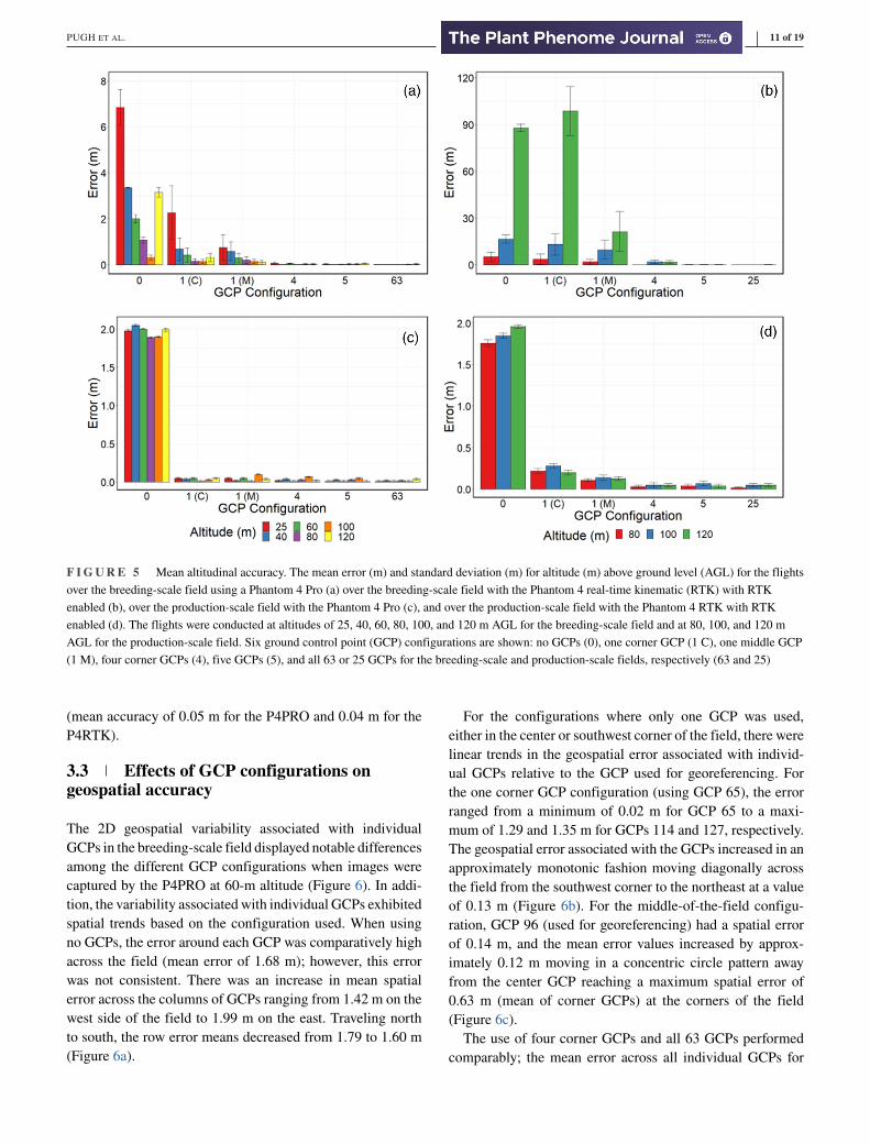
3.3 Effects of GCP configurations ongeospatial accuracy

The 2D geospatial variability associated with individual

GCPs in the breeding-scale field displayed notable differences

among the different GCP configurations when images were

captured by the P4PRO at 60-m altitude (Figure 6). In addi-

tion, the variability associated with individual GCPs exhibited

spatial trends based on the configuration used. When using

no GCPs, the error around each GCP was comparatively high

across the field (mean error of 1.68 m); however, this error

was not consistent. There was an increase in mean spatial

error across the columns of GCPs ranging from 1.42 m on the

west side of the field to 1.99 m on the east. Traveling north

to south, the row error means decreased from 1.79 to 1.60 m

(Figure 6a).

For the configurations where only one GCP was used,

either in the center or southwest corner of the field, there were

linear trends in the geospatial error associated with individ-

ual GCPs relative to the GCP used for georeferencing. For

the one corner GCP configuration (using GCP 65), the error

ranged from a minimum of 0.02 m for GCP 65 to a maxi-

mum of 1.29 and 1.35 m for GCPs 114 and 127, respectively.

The geospatial error associated with the GCPs increased in an

approximately monotonic fashion moving diagonally across

the field from the southwest corner to the northeast at a value

of 0.13 m (Figure 6b). For the middle-of-the-field configu-

ration, GCP 96 (used for georeferencing) had a spatial error

of 0.14 m, and the mean error values increased by approx-

imately 0.12 m moving in a concentric circle pattern away

from the center GCP reaching a maximum spatial error of

0.63 m (mean of corner GCPs) at the corners of the field

(Figure 6c).

The use of four corner GCPs and all 63 GCPs performed

comparably; the mean error across all individual GCPs for

12 of 19 PUGH ET AL.

F I G U R E 6 Geospatial accuracy of

individual ground control points (GCPs) Using

the Phantom 4 PRO. Spatial distribution of

georeferencing accuracy among GCPs in five

different GCPs configurations for flights

performed over the breeding-scale field at 60 m

above ground level. The radii of the circles

represent the error of each GCP increased by

adding a constant of 1 m for visual

enhancement. Five GCP configurations are

shown: no GCPs (a); one corner GCP, 65(b);

one middle GCP, 96 (c); four corner GCPs, 5,

71, 121, 127 (d); and all 63 GCPs (e). Green

indicates selected GCPs for georeferencing,

except for E where all 63 were used

both configurations was 0.03 m and both configurations had a

standard deviation of 0.02 m (Figure 6d, 6e). The mean error

for both rows and columns ranged from 0.02 to 0.04 m and

0.01 to 0.04 m, respectively, with no apparent spatial trend

in how errors were distributed, suggesting that the spatial

error was consistent throughout the field area in both con-

figurations. The geospatial variability associated with indi-

vidual GCPs from the P4RTK flights of the breeding-scale

flight at 60-m altitude did not exhibit significant differences

amongst the configurations tested nor were any spatial trends

apparent in the errors associated with GCPs across the field

area (Supplemental Figure S1). When no GCPs were used, the

mean spatial error associated with both the rows and columns

of GCPs was 0.06 m with minimal variation among them

(SD = 0.01 m; Supplemental Figure S1A). The one-corner

and middle-of-the-field GCP configurations performed simi-

larly; the mean error for both rows and columns of GCPs were

0.06 and 0.05 m, respectively, with no trend among the indi-

vidual rows/columns. The configurations utilizing the four

corner GCPs and all 63 of the GCPs produced similar results,

where mean spatial error across both rows and columns of

GCPs was 0.03 m with no observable trends across the field

in either direction highlighting the spatial consistency of the

georeferencing capabilities of the P4RTK.

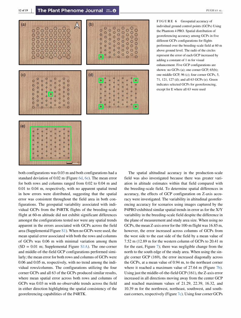
The spatial altitudinal accuracy in the production-scale

field was also investigated because there was greater vari-

ation in altitude estimates within that field compared with

the breeding-scale field. To determine spatial differences in

accuracy, the effects of GCP configuration on Z-axis accu-

racy were investigated. The variability in altitudinal georefer-

encing accuracy for scenarios using images captured by the

P4PRO exhibited similar spatial trends in error as for the X/Y

variability in the breeding-scale field despite the difference in

the plane of measurement and study area size. When using no

GCPs, the mean Z-axis error for the 100-m flight was 16.85 m,

however, the error increased across columns of GCPs from

the west side to the east side of the field by a mean value of

7.52 m (12.89 m for the western column of GCPs to 20.41 m

for the east, Figure 7); there was negligible change from the

north to the south edge of the study area. When using the sin-

gle corner GCP (169), the error increased diagonally across

the GCPs, at a mean value of 0.94 m, to the northeast corner

where it reached a maximum value of 27.64 m (Figure 7b).

Using just the middle-of-the-field GCP (161), the Z-axis error

increased in all directions moving away from the center GCP

and reached maximum values of 21.29, 22.39, 16.32, and

10.39 m for the northwest, northeast, southwest, and south-

east corners, respectively (Figure 7c). Using four corner GCPs

PUGH ET AL. 13 of 19

F I G U R E 7 Altitudinal accuracy for individual ground control points (GCPs) using the Phantom 4 Pro. Spatial distribution of georeferencing

accuracy for altitude among GCPs in five different GCPs configurations for flights performed over the production-scale field at 100 m above ground

level using the Phantom 4 Pro small unoccupied aircraft system (sUAS). The radii of the circles represent the altitudinal error of each GCP increased

by adding a constant of 10 m for visual enhancement. Five GCP configurations are shown: no GCPs (a); one corner GCP, 169 (b); one middle GCP,

161 (c); four corner GCPs, 149, 153, 169, 173 (d); and all 25 GCPs (e). Green indicates selected GCPs for georeferencing, except for E where all 25

were used

resulted in a mean Z-axis error of 1.98 m across the field, but

with respect to rows and columns, there were spatial trends.

Moving south to north (row 1 to row 5, respectively) across

rows of GCPs, mean Z-axis errors increased from 0.94 m for

row 1 to 3.03 m for row 3, and then finally back to 0.95 m

for row 5. This same trend was observed across columns of

GCPs as well; column 1 on the west side of the field had

a mean error of 1.01 m increasing to 2.87 m for column 3,

and finally 1.17 m for column 5 on the east side of the field

(Figure 7d). Finally, when all GCPs were used for processing,

the Z-axis mean error was 0.05 m, which was consistent across

the field without any trends or patterns observed (Figure 7e).

For the Z-axis error estimates from the imagery col-

lected with the P4RTK with RTK enabled, there were no

observed spatial trends in the altitudinal errors associated

with the individual GCPs for any of the GCP configura-

tions (Supplemental Figure S2). In fact, with respect to

row and column error means within each configuration, the

obtained mean altitudinal error values were nearly identical.

The only observed differences for mean error accuracy were

those associated with different GCP configurations discussed

above.

3.4 Validation of breeding-scale fieldaccuracy estimates

To assess the consistency of error estimates, a second set of

flights was conducted on the breeding-scale field in January of

2020 using the P4RTK with RTK both disabled and enabled

14 of 19 PUGH ET AL.

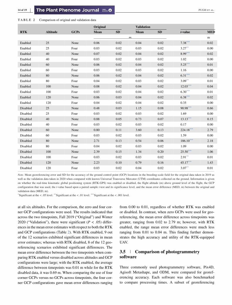
T A B L E 2 Comparison of original and validation data

Original ValidationRTK Altitude GCPs Mean SD Mean SD t-value MED

m m

Enabled 25 None 0.06 0.02 0.04 0.02 7.38*** 0.02

Enabled 25 Four 0.03 0.02 0.03 0.02 3.27** 0.00

Enabled 40 None 0.07 0.02 0.04 0.02 8.99*** 0.02

Enabled 40 Four 0.03 0.02 0.03 0.02 1.02 0.00

Enabled 60 None 0.06 0.02 0.04 0.02 5.25*** 0.01

Enabled 60 Four 0.03 0.02 0.03 0.02 1.16 0.00

Enabled 80 None 0.06 0.02 0.04 0.02 6.31*** 0.02

Enabled 80 Four 0.04 0.02 0.03 0.02 3.09** 0.01

Enabled 100 None 0.08 0.02 0.04 0.02 12.03*** 0.04

Enabled 100 Four 0.03 0.02 0.04 0.02 6.30*** 0.01

Enabled 120 None 0.06 0.03 0.04 0.02 6.38*** 0.02

Enabled 120 Four 0.04 0.02 0.04 0.02 0.35 0.00

Disabled 25 None 0.48 0.03 1.15 0.08 90.98*** 0.66

Disabled 25 Four 0.03 0.02 0.03 0.02 1.69 0.00

Disabled 40 None 0.88 0.05 0.73 0.07 13.13*** 0.15

Disabled 40 Four 0.03 0.02 0.03 0.02 0.17 0.00

Disabled 60 None 0.80 0.11 3.60 0.13 224.18*** 2.79

Disabled 60 Four 0.03 0.02 0.03 0.02 1.59 0.00

Disabled 80 None 2.71 0.13 0.54 0.06 186.10*** 2.18

Disabled 80 Four 0.04 0.02 0.03 0.02 1.09 0.00

Disabled 100 None 2.39 0.15 1.34 0.20 25.50*** 1.06

Disabled 100 Four 0.03 0.02 0.03 0.02 2.91** 0.01

Disabled 120 None 2.23 0.10 0.79 0.16 45.17*** 1.43

Disabled 120 Four 0.03 0.02 0.04 0.02 3.07** 0.01

Note. Mean georeferencing error and SD for the accuracy of the ground control point (GCP) locations in the breeding-scale field for the original data taken in 2019 as

well as the validation data taken in 2020 when compared with known Universal Transverse Mercator (UTM) coordinates collected on the ground. Information is given

on whether the real-time kinematic global positioning system (RTK-GPS) was enabled or disabled, the flight altitude (m) above ground level of the flight, the GCP

configuration that was used, the t-value based upon a paired sample t-test and its significance level, and the mean error difference (MED, m) between the original and

validation data (MED, m).*Significant at the < .05 level. **Significant at the < .01 level. ***Significant at the < .001 level.

at all six altitudes. For the comparison, the zero and four cor-

ner GCP configurations were used. The results indicated that

across the two timepoints, Fall 2019 (“Original”) and Winter

2020 (“Validation”), there were significant (P < .05) differ-

ences in the mean error estimates with respect to both the RTK

and GCP configurations (Table 2). With RTK enabled, 9 out

of the 12 scenarios exhibited significant differences in mean

error estimates; whereas with RTK disabled, 8 of the 12 geo-

referencing scenarios exhibited significant differences. The

mean error difference between the two timepoints when com-

paring RTK enabled versus disabled across altitudes and GCP

configurations were large; with the RTK enabled, the average

difference between timepoints was 0.01 m while for the RTK

disabled data, it was 0.69 m. When comparing the use of four

corner GCPs versus no GCPs across timepoints, the four cor-

ner GCP configurations gave mean error differences ranging

from 0.00 to 0.01, regardless of whether RTK was enabled

or disabled. In contrast, when zero GCPs were used for geo-

referencing, the mean error difference across timepoints was

greater, ranging from 0.02 to 2.79 m; however, with RTK

enabled, the range mean error differences were much less

ranging from 0.01 to 0.04 m. This finding further demon-

strates the high accuracy and utility of the RTK-equipped

UAV.

3.5 Comparison of photogrammetrysoftware

Three commonly used photogrammetry software, Pix4D,

Agisoft Metashape, and ODM, were compared for georef-

erencing accuracy. Each software was also benchmarked

to compare processing times. A subset of georeferencing

PUGH ET AL. 15 of 19

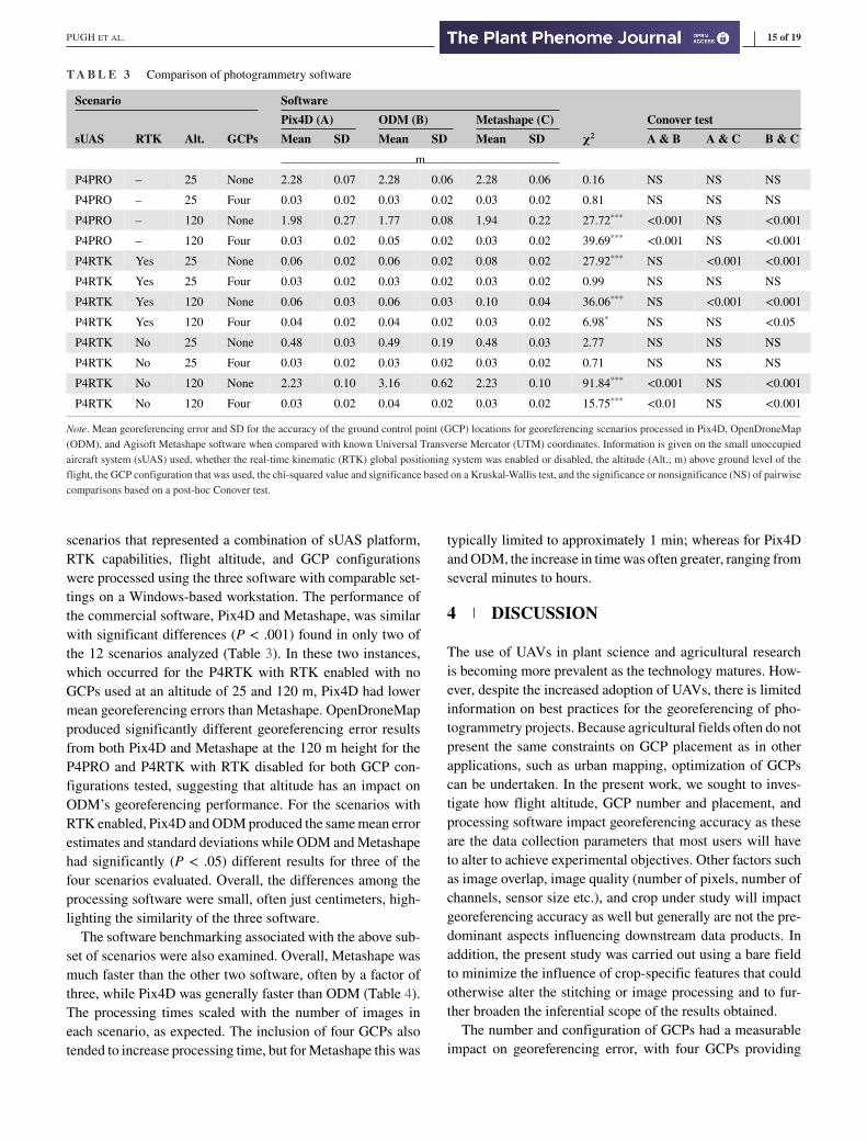
T A B L E 3 Comparison of photogrammetry software

Scenario SoftwarePix4D (A) ODM (B) Metashape (C) Conover test

sUAS RTK Alt. GCPs Mean SD Mean SD Mean SD χ2 A & B A & C B & Cm

P4PRO – 25 None 2.28 0.07 2.28 0.06 2.28 0.06 0.16 NS NS NS

P4PRO – 25 Four 0.03 0.02 0.03 0.02 0.03 0.02 0.81 NS NS NS

P4PRO – 120 None 1.98 0.27 1.77 0.08 1.94 0.22 27.72***<0.001 NS <0.001

P4PRO – 120 Four 0.03 0.02 0.05 0.02 0.03 0.02 39.69***<0.001 NS <0.001

P4RTK Yes 25 None 0.06 0.02 0.06 0.02 0.08 0.02 27.92*** NS <0.001 <0.001

P4RTK Yes 25 Four 0.03 0.02 0.03 0.02 0.03 0.02 0.99 NS NS NS

P4RTK Yes 120 None 0.06 0.03 0.06 0.03 0.10 0.04 36.06*** NS <0.001 <0.001

P4RTK Yes 120 Four 0.04 0.02 0.04 0.02 0.03 0.02 6.98* NS NS <0.05

P4RTK No 25 None 0.48 0.03 0.49 0.19 0.48 0.03 2.77 NS NS NS

P4RTK No 25 Four 0.03 0.02 0.03 0.02 0.03 0.02 0.71 NS NS NS

P4RTK No 120 None 2.23 0.10 3.16 0.62 2.23 0.10 91.84***<0.001 NS <0.001

P4RTK No 120 Four 0.03 0.02 0.04 0.02 0.03 0.02 15.75***<0.01 NS <0.001

Note. Mean georeferencing error and SD for the accuracy of the ground control point (GCP) locations for georeferencing scenarios processed in Pix4D, OpenDroneMap

(ODM), and Agisoft Metashape software when compared with known Universal Transverse Mercator (UTM) coordinates. Information is given on the small unoccupied

aircraft system (sUAS) used, whether the real-time kinematic (RTK) global positioning system was enabled or disabled, the altitude (Alt.; m) above ground level of the

flight, the GCP configuration that was used, the chi-squared value and significance based on a Kruskal-Wallis test, and the significance or nonsignificance (NS) of pairwise

comparisons based on a post-hoc Conover test.

scenarios that represented a combination of sUAS platform,

RTK capabilities, flight altitude, and GCP configurations

were processed using the three software with comparable set-

tings on a Windows-based workstation. The performance of

the commercial software, Pix4D and Metashape, was similar

with significant differences (P < .001) found in only two of

the 12 scenarios analyzed (Table 3). In these two instances,

which occurred for the P4RTK with RTK enabled with no

GCPs used at an altitude of 25 and 120 m, Pix4D had lower

mean georeferencing errors than Metashape. OpenDroneMap

produced significantly different georeferencing error results

from both Pix4D and Metashape at the 120 m height for the

P4PRO and P4RTK with RTK disabled for both GCP con-

figurations tested, suggesting that altitude has an impact on

ODM’s georeferencing performance. For the scenarios with

RTK enabled, Pix4D and ODM produced the same mean error

estimates and standard deviations while ODM and Metashape

had significantly (P < .05) different results for three of the

four scenarios evaluated. Overall, the differences among the

processing software were small, often just centimeters, high-

lighting the similarity of the three software.

The software benchmarking associated with the above sub-

set of scenarios were also examined. Overall, Metashape was

much faster than the other two software, often by a factor of

three, while Pix4D was generally faster than ODM (Table 4).

The processing times scaled with the number of images in

each scenario, as expected. The inclusion of four GCPs also

tended to increase processing time, but for Metashape this was

typically limited to approximately 1 min; whereas for Pix4D

and ODM, the increase in time was often greater, ranging from

several minutes to hours.

4 DISCUSSION

The use of UAVs in plant science and agricultural research

is becoming more prevalent as the technology matures. How-

ever, despite the increased adoption of UAVs, there is limited

information on best practices for the georeferencing of pho-

togrammetry projects. Because agricultural fields often do not

present the same constraints on GCP placement as in other

applications, such as urban mapping, optimization of GCPs

can be undertaken. In the present work, we sought to inves-

tigate how flight altitude, GCP number and placement, and

processing software impact georeferencing accuracy as these

are the data collection parameters that most users will have

to alter to achieve experimental objectives. Other factors such

as image overlap, image quality (number of pixels, number of

channels, sensor size etc.), and crop under study will impact

georeferencing accuracy as well but generally are not the pre-

dominant aspects influencing downstream data products. In

addition, the present study was carried out using a bare field

to minimize the influence of crop-specific features that could

otherwise alter the stitching or image processing and to fur-

ther broaden the inferential scope of the results obtained.

The number and configuration of GCPs had a measurable

impact on georeferencing error, with four GCPs providing

16 of 19 PUGH ET AL.

T A B L E 4 Software benchmarking for three photogrammetry programs

sUAS RTK AltitudeNo. ofimages

GCPconfiguration Pix4Dmapper OpenDroneMap Metashape

P4PRO N/A 25 374 None 2:50 13:57 1:31

P4PRO N/A 25 Four 3:37 16:00 1:30

P4PRO N/A 120 30 None 0:15 00:21 0:05

P4PRO N/A 120 Four 0:22 00:26 0:06

P4RTK Enabled 25 371 None 2:59 09:15 1:47

P4RTK Enabled 25 Four 4:50 10:33 1:48

P4RTK Enabled 120 43 None 0:20 00:26 0:06

P4RTK Enabled 120 Four 0:42 00:32 0:05

P4RTK Disabled 25 372 None 4:05 17:13 1:49

P4RTK Disabled 25 Four 4:09 19:27 1:51

P4RTK Disabled 120 43 None 1:08 00:30 0:08

P4RTK Disabled 120 Four 1:04 00:41 0:08

Note. Software benchmarking (hs:min) for each georeferencing scenario using three different photogrammetry software, Pix4Dmapper, OpenDroneMap, or Agisoft

Metashape. Shown is the small unoccupied aircraft system (sUAS) used for the flight, whether the real-time kinematic (RTK) global positioning system was enabled

or disabled, the altitude (m) above ground level, the ground control point (GCP) configuration that was used, and the total processing time for each georeferencing

scenario. sUAS, small unoccupied aircraft system.

optimal performance considering the ease of implementation

as well as performance across altitude and sUAS platforms.

When using no GCPs or only one GCP in either the corner or

middle of the field, the error was high and spatially variable

across the field, which roughly corresponded to the GCP con-

figuration used. In contrast, when four or more GCPs were

used, these patterns of spatial error were diminished or dis-

appeared entirely (Figures 6 and 7). Interestingly, geospatial

error was the highest in cases where only one GCP was used

rather zero GCPs. One hypothesis for why this occurred was

that the use of one geotagged GCP being used for georefer-

encing is not enough to adequately triangulate a position and

merely results in a translational shift of the imagery without

appropriate scaling. When using only one GCP, distortions

could be introduced due to this lack of scaling and the image

set could be “pulled” to the known coordinates of the single

GCP, as the image can be only be translated. The error when

using one GCP was often larger than when using no GCPs,

because georeferencing for the no GCP case was based on the

geotagged positioning data from the metadata of each image,

as recorded during the flight. Although this positioning data

were less accurate than the GCP positioning data, particularly

for the P4PRO and for the P4RTK with RTK disabled, it per-

mitted georeferencing with rescaling and therefore often led to

smaller georeferencing error than when using one GCP with

high positioning accuracy.

Based on the results presented for sUAS not equipped with

RTK, researchers that need centimeter-level georeferencing

accuracy only require four GCPs placed at the corners of the

study area regardless of flight altitude. This finding contrasts

with those reported in Oniga et al. (2020), wherein it was

found that using more GCPs could further improve results

until a plateau was reached when placing and using 20 GCPs

(Oniga et al., 2020). However, that study was conducted over a

∼1 ha urban area, and thus may not directly compare with the

present study, in which comparatively flat agricultural fields

were the focus. Given that Oniga et al. (2020) and the present

study have different visual features, this discrepancy is not sur-

prising (Oniga et al., 2020). In the present study, the threshold

reached upon using four GCPs holds true for the breeding-

scale field as well as the production-scale field, which indi-

cates that four georeferenced points should be sufficient and

allow centimeter-level accuracy in many common agricul-

tural scenarios, including at production-scale when compar-

ing large growing areas as well as at breeding-scale when

attempting to estimate specific phenotypes.

The use of the P4RTK with RTK enabled showed up to

25-fold reductions in spatial error as compared with the sce-

narios using the P4PRO. The accuracy of the scenarios using

RTK technology did improve in some cases with the addition

of GCPs, particularly regarding altitudinal accuracy; however,

the 2D accuracy was sufficient in most cases without the addi-

tion of any georeferenced points. The reduction in error in the

2D plane that was observed when using GCPs with the RTK

scenarios was minimal (Figures 4b and 5b). In addition, the

geospatial patterns of error associated with individual GCPs

that were observed in scenarios without RTK were greatly

minimized or removed entirely when using the P4RTK with

RTK enabled. The improvements in 3D accuracy were more

substantial for these scenarios when adding even just one GCP

(Figure 5b, 5d). These findings indicate that researchers that

have the resources to afford and implement a sUAS equipped

with RTK technology can forgo using GCPs altogether if their

only concern is the accuracy of objects in the 2D plane, and

PUGH ET AL. 17 of 19

they need only use one GCP to provide centimeter-level alti-

tudinal accuracy.

Remote sensing professionals that wish to use photogram-

metry for agricultural applications require software that can

perform the required tasks accurately and efficiently. As such,

analysis of three popular photogrammetry software packages

determined that there were key differences in their perfor-

mance (Tables 3 and 4). While Pix4Dmapper and Agisoft

Metashape performed most similarly of the three software

regarding processing benchmarks, ODM often took much

longer to process the same scenarios (Table 4). In similar fash-

ion, the georeferencing results of the three software packages

were different, with Pix4Dmapper and Metashape performing

most similarly, and ODM and Metashape showing the highest

number of significant differences in results (Table 3). Despite

these differences in processing benchmarks and performance,

it is important to note that ODM is open access, deployable

from the command line, and does not have licensing fees when

using the command line version, making it a viable option

for professionals that want accurate results without financial

input.

5 CONCLUSIONS

When using sUAS-based photogrammetry for agricultural

applications, a sufficient number and configuration of GCPs

is to use four locations in the corners of the field for proper

georeferencing. It is also important to note that using the entire

set of GCPs in either field offered virtually no increase in

accuracy along the X and Y planes and showed only minor

improvements along the Z plane. For sUAS equipped with

RTK, the technology can provide accurate georeferencing

with error less than 7 cm without need for GCPs; however,

GCPs should be used with an RTK-equipped sUAS if accu-

racy below 4 cm is required, such as in a breeding trial. Con-

versely, GCPs are likely not necessary at the production-scale

when an RTK-enabled sUAS is available, because researchers

and producers are often looking for differences on a larger

scale and the accuracy of RTK-enabled sUAS without GCPs

is likely sufficient. In summary, (a) no more than four GCPs

placed at the field corners are needed for centimeter-level

accuracy in the georeferencing of sUAS data at typical breed-

ing and production scales, (b) RTK-enabled sUAS have poten-

tial for accurate data without GCPs, and (c) available software

options are comparable, and choice depends on user prefer-

ence and available funds.

A C K N O W L E D G M E N T SThe authors would like to thank Sebastian Calleja, Matthew

Hagler, Suzette Maneely, and Bruno Rozzi for their direct con-

tributions to this study. Funding was provided Yuma Center of

Excellence Small Grants Program (Project #2019-04), Cotton

Incorporated (Project #17-642, Project #18-384), and Univer-

sity of Arizona Start Up Funds.

AU T H O R C O N T R I B U T I O N SN. Ace Pugh: Conceptualization; Data curation; Formal anal-

ysis; Investigation; Methodology; Software; Validation; Visu-

alization; Writing-original draft; Writing-review & editing.

Kelly R. Thorp: Conceptualization; Data curation; Formal

analysis; Investigation; Methodology; Resources; Supervi-

sion; Validation; Writing-review & editing. Emmanuel M.

Gonzalez: Formal analysis; Investigation; Software; Valida-

tion; Visualization; Writing-review & editing. Diaa Eldin

M. Elshikha: Data curation; Investigation; Methodology;

Resources; Validation; Writing-review & editing. Duke

Pauli: Conceptualization; Formal analysis; Funding acqui-

sition; Investigation; Methodology; Project administration;

Resources; Supervision; Validation; Visualization; Writing-

original draft; Writing-review & editing.

C O N F L I C T S O F I N T E R E S TThe authors declare no conflict of interest.

O R C I DN. Ace Pugh https://orcid.org/0000-0001-7129-6556

Kelly R. Thorp https://orcid.org/0000-0001-9168-875X

Emmanuel M. Gonzalez https://orcid.org/0000-0002-

3021-9842

Duke Pauli https://orcid.org/0000-0002-8292-2388

R E F E R E N C E SAgüera-Vega, F., Carvajal-Ramírez, F., & Martínez-Carricondo, P.

(2017). Assessment of photogrammetric mapping accuracy based

on variation ground control points number using unmanned aerial

vehicle. Measurement: The Journal of International MeasurementConfederation, 98, 221–227. https://doi.org/10.1016/j.measurement.

2016.12.002

Anderson, S. L., Murray, S. C., Malambo, L., Ratcliff, C., Popescu, S.,

Cope D., Chang A., Jung J., & Thomasson J. A. (2019). Prediction

of maize grain yield before maturity using improved temporal height

estimates of unmanned aerial systems. The Plant Phenome Journal,2(1), 1–15. https://doi.org/10.2135/tppj2019.02.0004

Araus, J. L., & Cairns, J. E. (2014). Field high-throughput phenotyping:

The new crop breeding frontier. Trends in Plant Science, 19(1), 52–

61. https://doi.org/10.1016/j.tplants.2013.09.008

Borra-Serrano, I., De Swaef, T., Quataert, P., Aper, J., Saleem, A., Saeys,

W., Somers B., Roldán-Ruiz, I., Lootens, P. (2020). Closing the phe-

notyping gap: High resolution UAV time series for soybean growth

analysis provides objective data from field trials. Remote Sensing,

12(10), 1644. https://doi.org/10.3390/rs12101644

Colomina, I., & Molina, P. (2014). Unmanned aerial systems for pho-

togrammetry and remote sensing: A review. ISPRS Journal of Pho-togrammetry and Remote Sensing, 92, 79–97. https://doi.org/10.1016/

J.ISPRSJPRS.2014.02.013

18 of 19 PUGH ET AL.

Ekaso, D., Nex, F., & Kerle, N. (2020). Accuracy assessment of real-

time kinematics (RTK) measurements on unmanned aerial vehicles

(UAV) for direct geo-referencing. Geo-spatial Information Science,

23(2), 165–181. https://doi.org/10.1080/10095020.2019.1710437

Fazeli, H., Samadzadegan, F., & Dadrasjavan, F. (2016). Evaluat-

ing the potential of RTK-UAV for automatic point cloud gen-

eration in 3D rapid mapping. In The International Archives ofthe Photogrammetry, Remote Sensing and Spatial Information Sci-ences, Volume XLI-B6, 2016 XXIII ISPRS Congress, 12–19 July2016, Prague, Czech Republic (pp. 221–226). International Society

for Photogrammetry and Remote Sensing. https://doi.org/10.5194/

isprsarchives-XLI-B6-221-2016

Forlani, G., Dall’Asta, E., Diotri, F., di Cella, U. M., Roncella, R., &

Santise, M. (2018). Quality assessment of DSMs produced from UAV

flights georeferenced with on-board RTK positioning. Remote Sens-ing, 10(2), 311. https://doi.org/10.3390/rs10020311

Forlani, G., Diotri, F., di Cella, U. M., & Roncella, R. (2019). Indirect

UAV strip georeferencing by on-board GNSS data under poor satel-

lite coverage. Remote Sensing, 11(15), 1765. https://doi.org/10.3390/

rs11151765

Gracia-Romero, A., Kefauver, S. C., Fernandez-Gallego, J. A., Vergara-

Díaz, O., Nieto-Taladriz, M. T., & Araus J. L. (2019). UAV and ground

image-based phenotyping: A proof of concept with durum wheat.

Remote Sensing, 11(10), 1244. https://doi.org/10.3390/rs11101244

Huang, Y., Brand, H. J., Sui, R., Thomson, S. J., Furukawa, T., & Ebel-

har, M. W. (2016). Cotton yield estimation using very high-resolution

digital images acquired with a low-cost small unmanned aerial vehi-

cle. Transactions of the ASABE, 59(6), 1563–1574. http://doi.org/10.

13031/trans.59.11831

Kawamura, K., Asai, H., Yasuda, T., Khanthavong, P., Soisouvanh, P.,

& Phongchanmixay, S. (2020). Field phenotyping of plant height

in an upland rice field in Laos using low-cost small unmanned

aerial vehicles (UAVs). Plant Production Science, 23(4), 452–465.

https://doi.org/10.1080/1343943X.2020.1766362

Li, F., Piasecki, C., Millwood, R. J., Wolfe, B., Mazarei, M., & Stew-

art, C. N., Jr. (2020). High-throughput switchgrass phenotyping

and biomass modeling by UAV. Frontiers in Plant Science, 11.

https://doi.org/10.3389/fpls.2020.574073

Malambo, L., Popescu, S. C., Murray, S. C., Putman, E., Pugh, N. A.,

Horne D. W., Richardson G., Sheridan R., Rooney W. L., Avant R.,

Vidrine M., McCutchen B., Baltensperger D., & Bishop M. (2018).

Multitemporal field-based plant height estimation using 3D point

clouds generated from small unmanned aerial systems high-resolution

imagery. International Journal of Applied Earth Observation andGeoinformation, 64, 31–42. https://doi.org/10.1016/J.JAG.2017.08.

014

Martínez-Carricondo, P., Agüera-Vega, F., Carvajal-Ramírez, F., Mesas-

Carrascosa, F. J., García-Ferrer, A., & Pérez-Porras, F.-J. (2018).

Assessment of UAV-photogrammetric mapping accuracy based on

variation of ground control points. International Journal of AppliedEarth Observation and Geoinformation, 72, 1–10. https://doi.org/10.

1016/j.jag.2018.05.015

Merkel, D. (2014). Docker: lightweight linux containers for consistent

development and deployment. Linux Journal, 2014(239), 2.

Obanawa, H., Sakanoue, S., & Yagi, T. (2019). Evaluating the applicabil-

ity of RTK-UAV for field management. In International Geoscienceand Remote Sensing Symposium (IGARSS) (pp. 9090–9092). Institute

of Electrical and Electronics Engineers.

Oniga, V. E., Breaban, A. I., Pfeifer, N., & Chirila, C. (2020). Deter-

mining the suitable number of ground control points for UAS images

georeferencing by varying number and spatial distribution. RemoteSensing, 12(5), 876. https://doi.org/10.3390/rs12050876

Pauli, D., Andrade-Sanchez, P., Carmo-Silva, A. E., Gazave, E., French,

A. N., Heun, J., Hunsaker, D. J., Lipka, A. E., Setter, T. L., Strand,

R. J., Thorp, K. R., Wang, S., White, J. W., & Gore, M. A. (2016).

Field-based high-throughput plant phenotyping reveals the tempo-

ral patterns of quantitative trait loci associated with stress-responsive

traits in cotton. G3 Genes. Genomes, Genet, 6(4), 865–879.

https://doi.org/10.1534/g3.115.023515

Pauli, D., Chapman, S. C., Bart, R., Topp, C. N., Lawrence-Dill, C.

J., Poland, J., & Gore, M. A. (2016). The quest for understanding

phenotypic variation via integrated approaches in the field environ-

ment. Plant Physiology, 172(2), 622–634. https://doi.org/10.1104/pp.

16.00592

Przybilla, H. J., Bäumker, M., Luhmann, T., Hastedt, H., & Eil-

ers, M. (2020). Interaction between direct georeferencing, con-

trol point configuration and camera self-calibration for RTK-based

UAV photogrammetry. The International Archives PhotogrammetryRemote Sensing and Spatial Information Sciences, 43(B1), 485–492.

https://doi.org/10.5194/isprs-archives-XLIII-B1-2020-485-2020

Pugh, N. A., Horne, D. W., Murray, S. C., Carvalho, G., Malambo, L.,

Jung, J., Chang A., Maeda, M., Popescu, S., Chu, T., Starek, M. J.,

Brewer, M. J., Richardson, G., & Rooney, W. L. (2018). Temporal

estimates of crop growth in sorghum and maize breeding enabled by

unmanned aerial systems. The Plant Phenome Journal, 1(1), 1–10.

https://doi.org/10.2135/tppj2017.08.0006

R Development Core Team. (2011). R: A language and environment forstatistical computing. R Core Team.

Rabah, M., Basiouny, M., Ghanem, E., & Elhadary, A. (2018). Using

RTK and VRS in direct geo-referencing of the UAV imagery. NRIAGJournal of Astronomy and Geophysics, 7(2), 220–226. https://doi.org/

10.1016/j.nrjag.2018.05.003

Ren, H., Zhao, Y., Xiao, W., Wang, X., & Sui, T. (2020). An improved

ground control point configuration for digital surface model construc-

tion in a coal waste dump using an unmanned aerial vehicle system.

Remote Sensing, 12(10), 1623. https://doi.org/10.3390/rs12101623

Sankaran, S., Khot, L. R., Espinoza, C. Z., Jarolmasjed, S., Sathuvalli,

V. R., Vandemark, G. J., Miklas, P. N., Carter, A. H., Pumphrey,

M. O., Knowles, N. R., & Pavek M. J. (2015). Low-altitude, high-

resolution aerial imaging systems for row and field crop pheno-

typing: A review. European Journal of Agronomy, 70, 112–123.

https://doi.org/10.1016/J.EJA.2015.07.004

Sanz-Ablanedo, E., Chandler, J., Rodríguez-Pérez, J., & Ordóñez, C.

(2018). Accuracy of unmanned aerial vehicle (UAV) and SfM

photogrammetry survey as a function of the number and loca-

tion of ground control points used. Remote Sensing, 10(10), 1606.

https://doi.org/10.3390/rs10101606

Schonberger, J. L., & Frahm, J. M. (2016). Structure-from-motion revis-

ited. In Proceedings of IEEE Conference on Computer Vision andPattern Recognition, Las Vegas, 27–30 June 2016 (pp. 4104–4113).

IEEE. https://doi.org/10.1109/CVPR.2016.445

Shi, Y., Thomasson, J. A., Murray, S. C., Pugh, N. A., Rooney, W.

L., Shafian, S., Rajan, N., Rouze, G., Morgan, C. L. S., Neely, H.

L., Rana, A., Bagavathiannan, M. V., Henrickson, J., Bowden, E.,

Valasek, J., Olsenholler, J., Bishop, M. P., Sheridan, R., Putman, E. B.,

. . . , Yang, C. (2016). Unmanned aerial vehicles for high-throughput

PUGH ET AL. 19 of 19

phenotyping and agronomic research. Plos One, 11(7), e0159781.

https://doi.org/10.1371/journal.pone.0159781

Singh, D., Wang, X., Kumar, U., Gao, L., Noor, M., Imtiaz, M., Singh, R.

P., & Poland, J. (2019). High-throughput phenotyping enabled genetic

dissection of crop lodging in wheat. Frontiers of Plant Science, 10,

394. https://doi.org/10.3389/fpls.2019.00394

Su, W., Zhang, M., Bian, D., Liu, Z., Huang, J., Wang, W., Wu, J., &

Guo, H. (2019). Phenotyping of corn plants using unmanned aerial

vehicle (UAV) images. Remote Sensing, 11(17), 2021. https://doi.org/

10.3390/rs11172021

Taddia, Y., Stecchi, F., & Pellegrinelli, A. (2019). Using DJI Phan-

tom 4 RTK drone for topographic mapping of coastal areas. Interna-tional Archives of the Photogrammetry, Remote Sensing and SpatialInformation Sciences, XLII-2/W13, 625–630. https://doi.org/10.5194/

isprs-archives-XLII-2-W13-625-2019

Terpilowski, M. (2019). scikit-posthocs: Pairwise multiple compari-

son tests in Python. Journal of Open Source Software, 4(36), 1169.

https://doi.org/10.21105/joss.01169

Thorp, K., Thompson, A., Harders, S., French, A., & Ward, R. (2018).

High-throughput phenotyping of crop water use efficiency via multi-

spectral drone imagery and a daily soil water balance model. RemoteSens, 10(11), 1682. https://doi.org/10.3390/rs10111682

Tonkin, T. N., & Midgley, N. G. (2016). Ground-control networks for

image based surface reconstruction: An investigation of optimum sur-

vey designs using UAV derived imagery and structure-from-motion

photogrammetry. Remote Sensing, 8(9), 786.

Villanueva, J. K. S., & Blanco, A. C. (2019). Optimization of ground

control point (GCP) configuration for unmanned aerial vehicle

(UAV) survey using structure from motion (SFM). The Interna-tional Archives of the Photogrammetry Remote Sensing and SpatialInformation Sciences, XLII-4/W12, 167–174. https://doi.org/10.5194/

isprs-archives-XLII-4-W12-167-2019

Virtanen, P., Gommers, R., Oliphant, T. E., Haberland, M., Reddy, T.,

Cournapeau, D., Burovski, E., Peterson, P., Weckesser, W., Bright, J.,

van der Walt, S. J., Brett, M., Wilson, J., Millman, K. J., Mayorov, N.,

Nelson, A. R. J., Jones, E., Kern, R., Larson, E., . . . , van Mulbregt, P.

(2020). SciPy 1.0: Fundamental algorithms for scientific computing

in Python. Nature Methods, 17(3), 261–272. https://doi.org/10.1038/

s41592-019-0686-2

Wang, J., Gea, Y., Heuvelink, G. B. M., Zhou, C., & Brus, D. (2012).

Effect of the sampling design of ground control points on the geo-

metric correction of remotely sensed imagery. International Journal

of Applied Earth Observation and Geoinformation, 18(1), 91–100.

https://doi.org/10.1016/j.jag.2012.01.001

Westoby, M. J., Brasington, J., Glasser, N. F., Hambrey, M. J., &

Reynolds, J. M. (2012). “Structure-from-motion” photogrammetry: A

low-cost, effective tool for geoscience applications. Geomorphology,

179, 300–314. https://doi.org/10.1016/j.geomorph.2012.08.021

Wickham, H. (2016). ggplot2: Elegant graphics for data analysis.

Springer-Verlag. https://ggplot2.tidyverse.org

Xie, C., & Yang, C. (2020). A review on plant high-throughput pheno-

typing traits using UAV-based sensors. Computers and Electronicsin Agriculture, 178, 105731. https://doi.org/10.1016/j.compag.2020.

105731

Yeom, J., Jung, J., Chang, A., Maeda, M., & Landivar, J. (2018). Auto-

mated open cotton boll detection for yield estimation using unmanned

aircraft vehicle (UAV) data. Remote Sens, 10(12), 1895. https://doi.

org/10.3390/rs10121895

Zhou, X., Zheng, H. B., Xu, X. Q., He, J. Y., Ge, X. K., Yao, X.,

Cheng, T., Zhu, Y., Cao, W. X., & Tian, Y. C. (2017). Predict-

ing grain yield in rice using multi-temporal vegetation indices from

UAV-based multispectral and digital imagery. ISPRS Journal of Pho-togrammetry and Remote Sensing, 130, 246–255. https://doi.org/10.

1016/j.isprsjprs.2017.05.003

Zimmerman, T., Jansen, K., & Miller, J. (2020). Analysis of UAS

flight altitude and ground control point parameters on DEM accuracy

along a complex, developed coastline. Remote Sensing, 12(14), 2305.

https://doi.org/10.3390/rs12142305

S U P P O R T I N G I N F O R M AT I O NAdditional supporting information may be found in the online

version of the article at the publisher’s website.

How to cite this article: Pugh, NA, Thorp, KR,

Gonzalez, EM, Elshikha, DEM, & Pauli, D.

Comparison of image georeferencing strategies for

agricultural applications of small unoccupied aircraft

systems. Plant Phenome J. 2021;4:e20026.

https://doi.org/10.1002/ppj2.20026