competition, cash holdings, and financing decisions - … · competition, cash holdings, and...

Competition, Cash Holdings, and Financing Decisions∗

Erwan Morellec† Boris Nikolov‡ Francesca Zucchi§

June 13, 2014

Abstract

We use a dynamic model of cash management in which firms face competitivepressure to show that competition increases corporate cash holdings as well asthe frequency and size of equity issues. In our model, these effects are drivenby small, financially constrained firms, in contrast with the theories based onstrategic interactions in which large leaders or incumbents value more cash. Wetest these predictions on Compustat firms for the period 1980-2007 and showthat product market competition has first order effects on the cash holdings andfinancing decisions of constrained firms, in ways consistent with our theory.

Keywords: product market competition; cash holdings; financing decisions.

JEL Classification Numbers: G32, G35.

∗First draft: 2009. This paper is based on a previous paper titled “Cash Holdings and Competition.”We thank Andrea Gamba, Dalida Kadyrzhanova, Michael Raith, Michael Roberts, Yuliy Sannikov,Ronnie Sircar, Norman Schurhoff, Clifford W. Smith, and seminar participants at Princeton University,the University of Lausanne, the University of Rochester, and the 2013 European Finance Associationmeetings for helpful comments. Erwan Morellec and Francesca Zucchi acknowledge financial supportfrom the Swiss Finance Institute.†Swiss Finance Institute, EPFL, and CEPR. E-mail: [email protected].‡University of Rochester. E-mail: [email protected]§Swiss Finance Institute and EPFL. E-mail: [email protected]

1 Introduction

In perfect capital markets, firms can instantly raise funds at no cost and there is no role

for internal capital. In the presence of capital market frictions, such as costs of raising

funds or capital supply uncertainty, survival or investment may depend on a firm’s cash

holdings. That is, when other sources of funds are costly, limited, or unavailable, firms

can use their cash holdings to fund capital expenditures or cover unexpected operating

losses to avoid inefficient closure. Consistent with this view, several studies report that

firms facing greater difficulties in obtaining external capital accumulate more cash and/or

save a greater fraction of their cash flow as cash (see e.g. Opler, Pinkowitz, Stulz, and

Williamson, OPSW 1999, or Almeida, Campello, and Weisbach, 2004).

Despite the substantial development of the literature on corporate cash holdings,

little attention has been paid so far to the effects of product market competition on

the decision to retain earnings or on the decision to issue securities for the purpose

of cash savings. Yet, since a monopolist is less likely to face financial difficulties than

a firm facing cutthroat competition, economic intuition suggests that product market

competition should be a prime determinant of these decisions. The purpose of this

paper is therefore twofold. First, we seek to understand when and how product market

competition affects corporate cash holdings. Second, we are interested in determining

its effects on the decision to issue equity for cash savings. To this end, we build a model

in which firms face competitive pressure and optimize their cash holdings as well as the

size and frequency of their equity issues. We then examine whether the predictions of

the model are supported by the data on firms’ cash management and financing decisions.

To develop our predictions on the relation between competition and cash holdings

and financing decisions, we start by formulating a model in which a firm operates a

set of assets that generate stochastic cash flows. In the model, the firm faces financing

constraints, in that raising outside funds to cover potential losses and avoid inefficient

1

closure is costly. The profitability of assets in place depends on the intensity of product

market competition and, hence, so does the risk that the firm will have to raise costly

external finance. Using this model, we show that the value of cash holdings increases

with the intensity of product market competition, so that firms should hold larger cash

balances and make larger equity issues when operating in more competitive industries.

We also demonstrate that product market competition has no bearings on cash holdings

or the size of equity issues in the absence of financing constraints. Lastly, we show that

even though product market competition increases target cash holdings and the size of

equity issues – which suggests that it should have a negative effect on the frequency

of equity issues – it also increases the frequency at which firms raise outside equity by

eroding firm profitability.

To test these predictions, we form a large sample of Compustat firms for the period

1980-2007. Our sample consists of 78,080 firm-year observations, in which industries

are defined using their 4-digit SIC code. For this sample, we estimate a series of cross-

sectional regressions relating cash holdings and the funds received from stock issues to

different measures of product market competition. In a first step of our analysis, we

estimate our empirical model on the full sample. In a second step, we re-estimate our

empirical specification on two subsamples comprising either financially constrained firms

or unconstrained firms. This allows us to assess the effects of financing constraints on

the relation between competition and cash holdings and financing decisions. To address

potential endogeneity concerns, we also estimate a series of IV regressions in which we

use import penetration as a measure of competition and instrument industry measures

of import penetration with import tariff rates and foreign exchange rates. Lastly, to test

our hypothesis on the relation between competition and the frequency of equity issues,

we estimate a mixed proportional hazard model relating product market competition to

a firm’s equity issuance hazard.

2

Our estimations reveal that cash holdings and equity issues are related to product

market competition in ways consistent with our theory. Notably, cash holdings are

positively associated with the intensity of product market competition as measured by

the price-to-cost margin of the firm (EPCM), the text based Herfindahl-Hirschman Index

(HHI TNIC), or the product market fluidity measure developed by Hoberg, Phillips,

and Prabhala (2012). The magnitude of the effect is substantial and larger than that

of firm characteristics, such as cash flow volatility, that have long been recognized as

prime determinants of cash management decisions. In addition, these results hold after

controlling for a host of variables. Also consistent with the model’s predictions, we

find that the association between competition and cash holdings is stronger for firms

facing greater financing constraints and that unconstrained firms’ cash holdings are not

systematically related to product market competition. Lastly, the IV approach confirms

our result that more competition results in higher cash holdings.

Turning to equity issues, our estimations reveal that a stronger competition results

in larger equity inflows. Here again, this result holds after controlling for a host of

variables, is stronger among firms facing tighter financing constraints, and is confirmed

by the IV approach. Because firms raise more funds when product market competition

is stronger, we could expect them to access capital markets less often. Yet, consistent

with our model’s prediction, we find that by eroding profitability competition increases

the frequency of equity issues. Notably, a one standard deviation decrease in the EPCM

measure results in an increase of the equity issuance hazard rate by 5.7%. If we measure

competition by HHI TNIC or fluidity, a one standard deviation increase in competition

results in an increase of the equity issuance hazard rate by 3.7% or 14.5%.

Our paper relates to the literature examining the relation between strategic interac-

tions and firms’ cash holdings and financing decisions. Most of the literature has either

tried to examine the effects of financial policies on predatory behavior (see e.g. Bolton

3

and Scharfstein, 1990, Chevalier, 1995, Kovenock and Phillips, 1997, or Campello, 2003)

or on potential entry by competitors (see Benoit, 1984, or Ma, Mello, and Wu, 2013).

The paper that is most closely related to ours in this literature is Fresard (2010) (see

also the recent papers by Fresard and Valta, 2013, and Lyandres and Palazzo, 2013).

In his empirical study, Fresard shows that larger relative-to-rivals cash reserves lead to

systematic future market share gains at the expense of industry rivals and that cash rich

firms may induce losses for financially weak firms and drive them out of the market,

thereby reducing competition. Thus, his empirical study suggests that cash policy com-

prises a substantial product market dimension and that there may be a negative relation

between the dispersion of cash holdings within an industry and the intensity of product

market competition.

Our paper complements the literature based on strategic interactions by showing

that there exists also an opposite, feedback effect of product market competition on the

level of cash holdings within an industry. Notably, our theoretical analysis demonstrates

that by reducing profitability, competition leads firms to hold more cash and to increase

the frequency and the size of their equity issues. Our empirical analysis shows that these

predictions are borne in the data and that the magnitude of the effects is substantial.

Importantly, theories in which cash holdings are motivated by purely strategic consider-

ations predict that large firms have greater incentives to hold cash and value more cash.

Indeed in these models, the value of cash typically arises due to a predatory motive or an

entry preemption motive and the firm engaging in predation or preemption is generally

the large or unconstrained incumbent. By contrast, our theory predicts that smaller and

more constrained firms facing competitive pressure value more cash. We find that this

prediction – that is unique to our model – is supported by the data.

Our paper also contributes to the line of research that uses dynamic models to exam-

ine the relation between product market competition and financing decisions. Several

4

papers examine the effects of competition on debt financing in oligopolies (see for ex-

ample Lambrecht, 2001, Morellec and Zhdanov, 2008, or Chu, 2012) or in perfectly

competitive industries (see Miao, 2005). However, to the best of our knowledge, there

is no paper in this literature that examines the relation between competition and firms’

financing and cash holdings decisions.

Lastly, our paper relates to the growing literature that uses dynamic models to

examine the determinants of corporate cash holdings (see for example Bolton, Chen,

and Wang, 2011, Decamps, Mariotti, Rochet, and Villeneuve, 2011, Boileau and Moyen,

2012, Hugonnier, Malamud, and Morellec, 2014, Eisfeldt and Muir, 2014, or Falato,

Kadhyrzanova, and Sim, 2013). The paper that is most closely related to ours in this

literature is Della Seta (2013). Della Seta examines the relation between cash holdings

and competition, assuming that firms cannot raise outside funds. By contrast, firms in

our model can raise outside funds, thereby allowing an analysis of the relation between

competition and financing decisions. In addition, Della Seta is a purely theoretical study

whereas our main focus is on the empirical relation between product market competition

and corporate decisions.

The paper is organized as follows. Section two describes the model and derives

our testable hypotheses. Section three describes the data. Section four presents our

empirical results. Section five concludes. All the proofs are gathered in the Appendix.

2 Model

2.1 Assumptions

Throughout the model, agents are risk-neutral and discount cash flows at a constant

rate ρ. We consider a set of i = 1, ..., n firms contemplating entry in an oligopolistic

market. Firms are ex-ante identical, and can produce a single consumption good with

5

their capital stock ki. Each unit of installed capital can produce one unit of output at a

cost Γ(qi) = γqi, where γ > 0 is the constant marginal cost of production. The produced

good is non-storable so that output equals demand. All the output is sold at a single

price, determined by the demand for the good and the total industry output, denoted

by Q = Σni qi. The inverse demand function of the industry is given by P (Q) = α − Q,

where α > 0 is a constant representing the maximum market clearing price (see Tirole,

1988 chapter 3, or Osborne, 2004 chapter 3). We assume that γ < α, to rule out cases

in which the marginal cost of production is always higher than the output price.

Each firm entering the industry chooses its output qi to maximize shareholder value,

given the output choice of its competitors. Firm i therefore installs the physical capital

ki = qi upon entry. (We examine the entry decision below.) Since all firms face the same

costs and demand function, we focus on a symmetric equilibrium in which firms initially

choose the same output level and commit to this level thereafter. Accordingly, we omit

the subscript i below.1 The operating cash flow of the firm at any time t > 0 increases

with the market clearing price P (Q), decreases with the marginal cost of production γ,

and is given by

dΠt = (P (Q)− γ) qdt+ σdWt

where σ is a positive constant and (Wt)t≥0 is a Brownian motion representing stochastic

shocks to cash flows. As in DeMarzo and Sannikov (2006) or DeMarzo, Fishman, He,

and Wang (2012), this specification implies that management controls the mean but not

1As firms do not adjust physical capital after entry, we focus on the open-loop Nash equilibrium of

our repeated Cournot game. In our model, initial investment in capital acts as a commitment device.

Indeed, because of the capacity constraint k?, firms cannot deviate and increase their output. It is not

optimal either to deviate and decrease output below q?, as this would increase the equilibrium price to

the benefit of the other firms in the industry. Therefore, any deviation from the maximum output q? is

suboptimal and the solution simplifies to the static Cournot game played at time zero, in which firms

initially decide on the equilibrium level of capital and output (see Fershtman and Kamien, 1987).

6

the volatility of the cash flow process Π.

Because of the Brownian shock W , the firm is exposed to potential operating losses

that can be covered either using cash reserves or by issuing new equity.2 Specifically,

we allow management to retain earnings inside the firm and denote by Ct the firm’s

cash holdings at any time t > 0. We assume that there is a cost of holding cash by

considering that cash reserves earn a constant interest rate r < ρ inside the firm. The

difference between ρ and r is a carry cost of liquidity.

We also allow the firm to increase its cash holdings or cover operating losses by raising

funds in the capital markets. We consider that when raising outside funds, the firm has

to pay a proportional cost p and a fixed cost f (see e.g. Altinkilic and Hansen, 2000,

or Kim, Palia, and Saunders, 2008, for evidence on issuance costs). Our specification

implies that when raising the amount (1 + p)ξ + f , the firm gets ξ. The net proceeds of

an issuance are then stored in the cash reserve, whose dynamics evolve as

dCt = rCtdt+ (P (Q)− γ) qdt+ σdWt − dDt + dGt − dΦt, Ct ≥ 0, (1)

where dDt represents the payouts to shareholders over the time interval [t, t + dt], dGt

represents the financing raised and dΦt represents issuance costs. Equation (1) shows

that cash reserves grow with earnings, with outside financing, and with the interest

earned on cash holdings and decrease with payouts to shareholders and issuance costs.

The firm can choose to abandon its assets at any time by distributing all of its cash.

Alternatively, it can be liquidated if its cash buffer reaches zero following a series of

negative shocks. We consider that the liquidation value of assets is given by θk? + Cτ ,

where 1− θ ∈ [0, 1] represents a liquidation cost and τ is the time of liquidation.

2The model can easily be extended to incorporate credit lines. Credit lines would allow the firm to

carry negative cash balances and would change the point at which firms issue equity. However, they

would have no qualitative effect on our predictions on the relation between product market competition

and firms’ cash holdings and financing decisions.

7

In the model, management acts in the best interest of shareholders and, conditional

on entering the industry, chooses the firm’s production (q), payout (D), financing (G),

and liquidation (τ) policies to maximize the present value of future dividends to incum-

bent shareholders. That is, management solves:

max(D,G,q,τ)

Ec[∫ τ

0

e−ρt (dDt − dGt) + e−ρτ (θk? + Cτ )

].

The first term in this expression represents the present value of payments to incumbent

shareholders until the liquidation time τ , net of the claim of new investors on future

cash flows. The second term represents the firm’s discounted liquidation value.

2.2 Solving management’s optimization problem

We solve the model using backward induction, i.e. starting with the value of a generic

firm in the industry, that we denote by V (c). We then use this value to derive the

condition under which entry is optimal.

To derive the value of an active firm, we start by assuming that issuance costs are

sufficiently low to guarantee that the condition

maxξ≥0{V (ξ)− (1 + p)ξ − f} > θk?, (2)

holds. Later in the analysis, we verify that this condition is always satisfied when firms

find it optimal to enter the industry. Under this condition, raising outside financing is

better than liquidating operations, because the continuation value net of the issuance

costs (the left hand side) is higher than firm value in liquidation (the right hand side).

In this case, the firm is infinitely lived and we have τ =∞. When this condition is not

satisfied, firms never raise funds and are liquidated as soon as c = 0.

When condition (2) is satisfied, management only needs to select the production,

payout, and financing policies that maximize the value of shareholders’ claim. Since

8

raising funds is costly and the only benefit of raising funds is to avoid liquidation,

management postpones equity issuances until cash reserves are exhausted (i.e. until

c = 0), as in Decamps, Mariotti, Rochet, and Villeneuve (2011). In addition, because

the marginal cost of cash holdings is constant and their marginal benefit is decreasing,

we conjecture that there exists some level C? for the cash buffer where the marginal cost

and benefit of cash holdings are equalized and it is optimal to start paying dividends.

Below C?, the optimal policy is to build up cash reserves by retaining earnings and to

raise outside funds when c = 0.

To solve for firm value, consider first the region (0, C?) over which it is optimal to

retain earnings. In this region, firm value satisfies:

ρV (c) = maxq≥0

{V ′(c) [rc+ (P (Q)− γ) q] +

σ2

2V ′′(c)

}. (3)

The left-hand side of this equation represents the required rate of return for investing in

the firm. The right-hand side is the expected change in firm value in the region where

the firm retains earnings. The first term captures the effects of cash savings on firm

value while the second one captures the effects of cash flow volatility.

The choice of production size q is made ex ante by management to maximize firm

value. The first order condition yields:

q? =α− γn+ 1

,

that is the static symmetric Nash solution when firms compete a la Cournot. Thus,

each firm installs k? = q? units of capital at time zero and total output in equilibrium is

Q = K = nn+1

(α− γ) < α−γ. This in turn guarantees a market clearing price given by

P (Q) =α + nγ

n+ 1= γ +

α− γn+ 1

,

and implies that the firm’s expected profit on any time interval [t, t+ dt] satisfies:

q? (P (Q)− γ) dt = k?α− γn+ 1

dt.

9

Plugging the expression for the expected profit of the firm in equation (3), we finally get

that firm value solves in the retention region (0, C?):

ρ V (c) =

[rc+ k?

α− γn+ 1

]V ′(c) +

σ2

2V ′′(c).

As long as the marginal value of cash is greater than one, it is optimal to retain

earnings. As cash reserves increase, the likelihood of costly equity financing decreases.

As a result, the marginal value of cash decreases until it reaches one and it is optimal

to start paying dividends. We then have the following boundary condition:

limc↑C?

V ′(c) = 1, (4)

where the value-maximizing dividend threshold C? satisfies the high-contact condition

limc↑C?

V ′′(c) = 0. (5)

If the firm has too much cash (i.e if c > C?), it is optimal to distribute all cash holdings

above C∗ with a specially designated dividend or a share repurchase and we have:

V (c) = V (C?) + c− C?.

Lastly, under condition (2), the firm raises equity every time its cash buffer is depleted

in order to avoid liquidation. Accordingly, the value-matching condition at zero is

V (0) = V (ξ?)− (1 + p)ξ? − f, (6)

implying that the value of the shareholders’ claim when raising outside financing is equal

to the continuation value less issuance costs. The value-maximizing amount of outside

financing ξ? is then determined by the first order condition:

V ′(ξ?) = 1 + p, (7)

which ensures that the marginal cost of outside funds is equal to the marginal benefits

of cash holdings at the post-issuance level of cash reserves.

Solving management’s optimization problem yields the following Proposition.

10

Proposition 1 The value V (c) of the financially constrained firm is given by

V (c) =

F ′′(C?)G(c)−G′′(C?)F (c)

2√rρ

σ3e(rC?+π?(n))2/(rσ2) if 0 ≤ c < C?

c− C? + V (C?) if c ≥ C?

where C? is the unique solution to equation (5), π?(n) ≡(α−γn+1

)2, the functions F and G

are defined in the Appendix, and firm value at the dividend threshold C? satisfies

V (C?) =1

ρ

{rC? + k?

α− γn+ 1

}.

In equilibrium, firm size is given by

k? =α− γn+ 1

,

and the size of new issues ξ? is the unique solution to equation (7).

Having derived the value of an active firm, we are now interested in determining

when entry is optimal. Suppose that firms have no cash initially. The optimal size of

the initial equity issue, given by ξ? + k?, is such that the marginal cost of outside funds

is equal to their marginal benefit and the entry condition can be written as

V (ξ?) ≥ (ξ? + k?) (1 + p) + f. (8)

Condition (8) implies that firms enter the industry as long as the fixed cost of raising

funds is below f defined by f ≡ V (ξ?) − (ξ? + k?) (1 + p). Lastly, note that condition

(8) implies that condition (2) holds since V (ξ?)− ξ?(1 + p)− f ≥ (1 + p)k? ≥ θk?. That

is, if a firm initially finds it profitable to enter the industry, it also finds it optimal to

raise funds whenever its cash buffer drops to zero instead of liquidating operations.3

3In our model, firms are symmetric and either all firms enter or no firm enters the market. Introducing

heterogeneity among firms through, e.g. asymmetric production costs as in Ledvina and Sircar (2012),

would allow us to get a richer industry structure. However, this would not change our predictions on

the relation between product market competition and cash holdings and financing decisions.

11

2.3 Empirical predictions

2.3.1 Optimal cash holdings

In the model, an active firm determines the optimal level of cash holdings by balancing

their cost with their benefits, i.e. the possibility to cover operating losses without having

to issue costly equity. As a result, a change in profitability – due to changes in n, α,

and γ – in the volatility of the cash flow shock σ, or in the costs of outside funds, p and

f , will lead to a change in the value-maximizing level of cash holdings C?. The follow-

ing Proposition provides a formal characterization of the effects of firm characteristics,

product market competition, and financing constraints on optimal cash holdings.

Proposition 2 Target cash holdings C? are increasing with cash flow volatility σ, the

number of firms in the industry n, the marginal cost of production γ, and issuance costs

p and f , and decreasing with firm size k? and the maximum clearing price α.

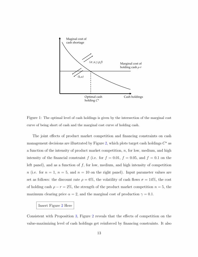
Figure 1 shows the marginal cost curve of being short of cash and the marginal cost

curve of holding cash. The marginal cost curve of being short of cash is downward

sloping and convex as the value of the firm is an increasing and concave function of

the firm’s cash reserves. The marginal cost of holding cash is constant, given by ρ− r.

Proposition 2 shows that an increase in product competition, in financing constraints, in

production costs, or in cash flow volatility shifts the marginal cost curve of being short

of cash to the right and increases the optimal level of cash holdings.

One question that naturally arises in our setup relates to the joint effects of product

market competition and financing constraints on target cash holdings. The following

Proposition provides a formal characterization of these effects.

Proposition 3 The effects of product market competition on target cash holdings in-

crease with the severity of financing constraints in that ∂2C?

∂n∂f> 0.

12

Marginal cost of holding cash ρ-r

Cash holdings

Maginal cost of cash shortage

Optimal cash holding C*

( ,n,γ,p,f)

(k,α)

Figure 1: The optimal level of cash holdings is given by the intersection of the marginal cost

curve of being short of cash and the marginal cost curve of holding cash.

The joint effects of product market competition and financing constraints on cash

management decisions are illustrated by Figure 2, which plots target cash holdings C? as

a function of the intensity of product market competition, n, for low, medium, and high

intensity of the financial constraint f (i.e. for f = 0.01, f = 0.05, and f = 0.1 on the

left panel), and as a function of f , for low, medium, and high intensity of competition

n (i.e. for n = 1, n = 5, and n = 10 on the right panel). Input parameter values are

set as follows: the discount rate ρ = 6%, the volatility of cash flows σ = 14%, the cost

of holding cash ρ− r = 2%, the strength of the product market competition n = 5, the

maximum clearing price α = 2, and the marginal cost of production γ = 0.1.

Insert Figure 2 Here

Consistent with Proposition 3, Figure 2 reveals that the effects of competition on the

value-maximizing level of cash holdings get reinforced by financing constraints. It also

13

shows that the effects of competition on cash holdings are quantitatively very strong.

In summary, our model produces the following unique predictions on corporate cash

holdings. First, as product market competition intensifies (as n increases), profitability

decreases and firms optimally respond by increasing their cash holdings. This leads to

the following testable hypothesis:

Hypothesis 1: Cash holdings increase with the strength of product market competition.

Second, when there are no financing constraints, firms can issue securities at no cost

and have no need for cash holdings. As financing constraints increase (i.e. as f increases),

the wedge between the costs of inside and outside equity increases. Firms optimally

respond by hoarding more cash. This leads to the following testable hypothesis:

Hypothesis 2: The effect of product market competition on optimal cash holdings

increases with the intensity of financing constraints.

At this stage it is important to note that theories in which cash holdings are motivated

by purely strategic considerations predict that large firms have greater incentives to hold

cash and value more cash. Indeed in these models, the value of cash typically arises due to

a predatory motive or an entry preemption motive and the firm engaging in predation

or preemption is generally the large or unconstrained leader or incumbent. Thus, a

distinguishing feature of our theory is that it predicts that smaller and more constrained

firms facing competitive pressure value more cash.

2.3.2 Financing decisions

When deciding on the size of equity issues, the firm balances the benefits of having

greater cash reserves following the issue with the costs of issuing equity. The follow-

ing Proposition provides a formal characterization of the effects of firm characteristics,

product market competition, and financing constraints on the size of equity issues.

14

Proposition 4 When issuing equity, the optimal issue size ξ? is increasing in cash

flow volatility σ, product market competition n, the marginal cost of production γ, and

issuance costs f , and decreasing in firm size k? and the maximum clearing price α.

The intuition underlying the effects of volatility, competition, firm size, marginal

costs of production, and the maximum clearing price on the optimal issue size is similar

to that underlying their effects on optimal cash holdings. The effect of fixed issuance

costs on the optimal issue size are related to the financing condition (2), which shows

that the larger f , the larger the amount that needs to be raised by the firm. Figure 2

illustrates the joint effects of competition and financing constraints on equity issues and

shows that the optimal issue size and target cash holdings respond in a similar fashion

to changes in the firm’s environment. We then have the following testable hypotheses:

Hypothesis 3: The optimal issue size increases with product market competition.

Hypothesis 4: The effect of product market competition on the optimal issue size

increases with the severity of financing constraints.

Another question of interest is whether product market competition affects the fre-

quency at which firms access financial markets and, therefore, the present value of is-

suance costs. Intuitively, the answer to this question is not clear since product market

competition has potentially two opposite effects on the frequency of equity issues. On

the one hand, competition increases target cash holdings and the size of equity issues,

which suggests that it should have a negative effect on the frequency of equity issues. On

the other hand, competition reduces profitability and hence makes it more likely that

the firm will make losses and will need to raise outside capital, everything else equal.

To address this question, we compute the probability of an equity issue over any given

horizon T > 0 as a function of the intensity of product market competition, defined as

P0 (t;T, c) ≡ P [τ0(C?) ≤ T |Ct = c] ,

15

where τ0(C?) is the first time that the cash reserves process with payouts at C? reaches

0. The Appendix shows how to compute this probability.


Figure 3 plots the probability of an equity issue as a function of the current cash

buffer (C ∈ [0.01, C?]) over an horizon of two (left panel) and five (right panel) years.

The solid line plots this probability for a monopolist (n = 1) while the long-dashed and

short-dashed lines plot these probabilities for industries with n = 5 and n = 10 firms,

respectively. Input parameter values are set as in Figure 2. Figure 3 shows that the

probability of an equity issue increases with competition (i.e. the profitability effect

dominates). As expected, this probability also increases with the horizon and decreases

with the financial strength of the firm, as measured by C.

This leads to the following testable hypothesis:

Hypothesis 5: Product market competition increases the frequency of equity issues.

In the remainder of the paper, we test hypotheses 1 through 5 on Compustat firms

for the period 1980-2007.

3 Data and methodology

3.1 Sample

Our sample of firms is based on Compustat Industrial Annual files. Following Bates,

Kahle and Stulz (BKS, 2009), we examine firms over the 1980-2007 period. We remove

firms from regulated industries (SIC 4900-4999) and financial firms (SIC 6000-6999). In

addition, following Clarke (1989), we remove firms with 4-digit SIC codes ending either

by 0 or 9 that group firms with not well defined industry. Observations with missing

16

SIC code, total assets, cash and short term investments, sales, and operating income are

deleted. We also drop observations with negative or zero total assets or sales, as well

as observations with a negative EBITDA larger than total assets (see Bris, Koskinen,

and Nilsson, 2009). The final sample consists of 78,080 firm-year observations, in which

industries are defined by their 4-digit SIC code.

We collect the data on imports, exports, and tariffs compiled by Feenstra (1996) and

Feenstra, Romalis, and Schott (2001). Data on imports, exports, and tariffs are avail-

able at the product level as defined by the Harmonized System (HS) established by the

World Customs Organization (WCO). Feenstra (1996) and Schott (2010) provide con-

cordance tables that map products to SIC codes. Using these tables, we define industry

level variables at the four-digit SIC level. These data are available for manufacturing

industries from 1980 to 1999. In addition, we collect data on domestic production from

the Bureau of Economic Analysis, data on foreign exchange rates from Datastream, and

data on Consumer Price Indices from the IMF. Finally, we collect data on firm industry

exposure from Compustat Segments.

3.2 Methodology

To test Hypotheses (1) and (2) on the relation between cash holdings and competition,

we estimate the following model:

Cashi,t = β1Competitionj,t−1 + β2FinConstrainti,t−1 + β3Yi,t−1 +ϕj + νt + εi,t. (9)

The subscripts i, j, and t represent firm, industry, and year, respectively. Equation (9)

relates cash holdings to the intensity of product market competition and the severity

of financing constraints. Competitionj,t−1 is the competition measure for industry j, in

year t−1, where firm i operates. FinConstrainti,t−1 is the financing constraint measure

for firm i at time t−1. Our main focus is on the coefficient estimates β1 and β2. The set

17

of control variables Yi,t−1 includes variables that are commonly believed to affect cash

holdings (see BKS, 2009, and OPSW, 1999). ϕj accounts for time-invariant industry

fixed effects. νt accounts for year fixed effects. The definition and construction of the

dependent, explanatory, and control variables are summarized in Table 1.

Insert Table 1 Here

In equation (9), cash holdings are measured as cash and short term investments

deflated by book assets, as in BKS. The cash ratio may be defined in various ways.

OPSW use cash deflated by book assets minus cash. Haushalter, Klasa, and Maxwell

(2008) use the log of the OPSW measure. The drawback of these measures is that they

generate extreme outliers. Unreported robustness checks show that our conclusions are

not affected by the definition of the dependent variable. Volatility is computed as the

mean of standard deviations of operating income before depreciation (OIBDP) deflated

by total assets (AT) over 10 years for firms in the same industry, as defined by the 4-digit

SIC code. Firm size is defined as the log of net sales (SALE).

Turning to the tests of Hypotheses (3) and (4) on the relation between issue size and

competition, we estimate the following model:

Issuei,t = β1Competitionj,t−1 +β2FinConstrainti,t−1 +β3Zi,t−1 +ϕj + νt + εi,t. (10)

The subscripts i, j, and t represent firm, industry, and year, respectively. In this equa-

tion, the set of control variables Zi,t−1 includes variables that are commonly believed to

affect equity issuances (see e.g. Baker and Wurgler, 2002, and McLean, 2011). Equity

issuances are defined as sales of common and preferred stock (SSTK) net of repurchase

(PRSTKC), deflated by total assets (AT). Therefore, Issuei,t represents funds received

from stock issuances at time t, as in McLean (2011). In unreported tests, we obtain

similar results when employing the net equity issues proxy in Baker and Wurgler (2002),

defined as the change in book equity minus the change in balance sheet retained earnings,

divided by assets.

18

In a first step, we estimate equations (9) and (10) to assess the effect of competi-

tion and financing constraints on cash and equity issues. In a second step, we examine

the effects of financing constraints by estimating the specification in equation (9) and

(10) when splitting the full sample in two subsamples comprising either financially con-

strained firms or unconstrained firms.

Finally, we also test Hypothesis (5) on the relation between the frequency of equity

issues and competition. To do so, we follow Leary and Roberts (2005) and estimate a

mixed proportional hazard model, for which the hazard function at time t for firm i with

covariates xi(t) is assumed to be

λi (t) = ωiλ0(t) exp(xi(t)′β). (11)

In this model, t is the time to equity issuance (or equivalently the length of the spell),

λ0(t) is the baseline hazard function, that we model as a non-parametric step function

of discrete spell lengths, and exp(xi(t)′β) is the relative risk associated with the set of

covariates xi(t). These covariates characterize observed differences between firms and β

is an unknown parameter vector. Lastly, ωi is a random variable representing unobserved

heterogeneity. We assume that the unobserved heterogeneity has a gamma distribution

with mean zero and variance s2. We estimate the model via maximum likelihood.

The baseline hazard is interpreted as the hazard function when all covariates are zero.

The covariates allow the hazard function to shift up or down depending on their values

and the parameter vector β. The covariates that we consider include our proxies for the

intensity of competition as well as control variables. ωi accounts for omitted covariates

so that the estimated hazard functions are not affected by unobserved heterogeneity.

Most firms in the Compustat dataset exhibit issuance activity every period. This

is in part due to continued exercise of stock options by executives (see McKeon, 2013).

For the duration analysis, we thus follow Leary and Roberts (2005) and focus on large

19

equity issues or spikes. An equity issuance spike occurs if equity issuance, defined as

sales of common and preferred stock (SSTK), deflated by total assets (AT), is greater

than 3%. In robustness tests, we change the equity issuance spike threshold to 5% or

7%. As an additional robustness test, we define equity issuance spikes in terms of the

deviation of the ratio of equity issuance to total assets from the firm level median of

this ratio (following Whited, 2006). This alternative definition for equity issuance spikes

does not have any material impact on our results.

3.3 Intensity of competition measures

We construct four measures to reflect the intensity of product market competition. First,

we use the excess price-cost margin (EPCM) (see e.g. Lindenberg and Ross, 1981,

Nickell, 1996, Aghion et al., 2005, or Gaspar and Massa, 2006). The price-cost margin

(PCM) is defined as operating income (before depreciation) over sales. EPCM is defined

as the difference between a firm’s PCM and the average PCM of its industry. We control

for industry PCM in order to account for inter-industry differences unrelated to market

power. In this specification, we assume that marginal and average costs are equivalent

(see Carlton and Perloff, 1989). The price-cost margin is used in most of the industrial

organization (IO) literature and refers to the ability of the firm to price above marginal

cost (see Lerner, 1934). A greater value of EPCM indicates a greater ability to extract

profits and, hence, a lower intensity of competition.

Our second proxy for the intensity of competition is the Herfindahl-Hirschman Index

(HHI). A higher HHI implies weaker competition. The HHI is a widely used proxy for

competition that is well grounded in industrial organization theory (see Tirole, 1988).

In our estimations, the HHI is based on the text-based network industry classification

(TNIC) available in the Hoberg and Phillips data library. This dynamic industry classifi-

cation is based on product descriptions from annual firm 10-K filings with the Securities

20

and Exchange Commission (SEC). Hoberg and Phillips (2011) use this new classification

and show that it is better at explaining the cross-section of firm characteristics (see also

Hoberg and Phillips, 2010). This proxy is available for the years 1996 to 2007.

Our third proxy for the intensity of competition is the product market fluidity mea-

sure developed by Hoberg, Phillips, and Prabhala (2012) and available in the Hoberg

and Phillips data library. Higher fluidity signals a more competitive environment. This

proxy is also based on business descriptions from firm 10-Ks and captures the structure

and evolution of the product space occupied by firms. In particular, it captures com-

petitive threats faced by firms in their product markets and the changes in rival firms’

products relative to the firm. This proxy is available for the years 1997 to 2007.

Lastly, we use foreign competition as measured by the degree of import penetration

(see Bertrand, 2004) to examine the effects of competition on cash holdings. Import

penetration (IP) is defined as total value of imports divided by imports plus domestic

production. In order to account for possible endogeneity between corporate decisions

and import penetration, we instrument import penetration with import tariffs and the

exchange rate. The ad valorem tariff rate is defined as the total value of duties collected

by the U.S. customs divided by the total free-on-board value of imports. The foreign ex-

change rate is the weighted average of the log real exchange rates of exporting countries.

It is expressed in foreign currency per U.S. dollar. The weights are defined as the share

of each foreign country exports over total imports. The real exchange rates are nominal

rates that are adjusted for the U.S and the foreign country Consumer Price Indices. All

measures are constructed at the four-digit SIC level. In addition, we compute firm level

measures. To do so, we construct weights for each firm that correspond to the fraction

of sales associated with each industry. The firm specific measures then correspond to

the weighed average of industry measures where the weights represent the exposure of

the firm to the industries it operates in.

21

3.4 Financing constraint measures

Financing constraints are unobservable at the firm level. As a result, empiricists have

proposed an array of methods to measure these constraints. Since there is no agreement

on which measure is the best proxy for financing constraints, we rely on four different

measures that complement each other.

The literature on financing constraints argues that a firm’s payout ratio may be

used to measure financial constraints (see Fazzari, Hubbard and Petersen, 1988). Thus,

for every year in our sample, we rank firms based on their payout ratio. Financially

constrained (unconstrained) firms are identified as being in the bottom (top) three deciles

of the annual payout ratio distribution. The payout ratio is defined as total distributions

(dividends and stock repurchases) deflated by operating income. All firms having the

same payout ratio are assigned to the same group.

The second measure we use for firms’ financing constraints is firm size (see Gilchrist

and Himmerlberg, 1995, and Erickson and Whited, 2000). Small firms are typically

young, less known, and more vulnerable to capital market imperfections and, thus, are

more likely to face financing difficulties. In addition, larger, more established firms

are more likely to have a well functioning treasury department and well established

relations with financial institutions rendering access to capital markets easier. For every

year, we rank firms based on their size. Financially constrained (unconstrained) firms

are identified as being in the bottom (top) three deciles of the annual size distribution.

Similar results are obtained if we use firm age instead of firm size.

We use the market assessment of firms’ credit risk as third measure of financing

constraints (see Whited, 1992, and Gilchrist and Himmelberg, 1995). We categorize firms

as financially constrained if the credit rating is either missing or non investment grade.

Financially unconstrained firms are firms with an investment grade rating. Similar

results are obtained if we use instead commercial paper rating.

22

We use the Whited and Wu financial constraints index as fourth measure (WW

index). Firms with high WW index are small firms, that rely mainly on equity financing,

exhibit low growth and have low cash flows. Formally, the index is defined as follows:

WW= −0.091CF−0.062DIVPOS+0.021TLTD−0.044LNTA+0.102ISG−0.035SG

where CF is cash flows from operations, DIVPOS is a dummy variable equal to 1 if the

firm pays dividends, TLTD is long term debt over assets, LNTA is the natural logarithm

of total assets, ISG is the three-digit SIC industry sales growth rate and SG is the firm

sales growth rate. We compute the WW index every year for each firm. Financially

constrained (unconstrained) firms are then identified as being in the top (bottom) three

deciles of the WW index annual distribution.

Insert Table 2 Here

Table 2 reports the number of firm-year observations classified as constrained or

unconstrained for the four financial constraints criteria. For example, there are 50,865

constrained firm-year observations and 25,937 unconstrained according to the payout

ratio criterion. Table 2 shows that the four criteria are positively but not perfectly

correlated. Indeed, out of the 50,865 payout constrained firm-year observations, 22,703

are considered constrained and 7,208 unconstrained with respect to the size criterion.

The remaining observations are considered as neither constrained nor unconstrained.

Each of the four measures of financing constraints thus conveys incremental information,

which contributes to the robustness of the analysis.

3.5 Descriptive statistics

Table 3 presents descriptive statistics of the sample. Our sample exhibits characteristics

similar to those in prior studies (see e.g. BKS, 2009, McLean, 2011, Hoberg, Phillips,

23

and Prabhala, 2013). Mean cash holdings are 0.17 with a standard deviation of 0.20,

whereas equity issues have a mean of 0.04 and a standard deviation of 0.13.

Insert Table 3 Here

The mean excess price-cost margin (EPCM), our first proxy for the intensity of

competition, is -0.17 with a standard deviation of 0.59. The mean EPCM is slightly

lower than those reported by Aghion et al. (2005) or Gaspar and Massa (2006) because

our sample period also includes more recent years. Turning to the Hoberg and Phillips

measures of competition, HHI TNIC has an average of 0.18 with a standard deviation

of 0.20, whereas product market fluidity is 7.30 with a standard deviation of 3.38. The

results are consistent with Hoberg, Phillips, and Prabhala (2013).


Figure 4 (left panel) plots firms’ cash holdings over the sample period. At the be-

ginning of the sample period in 1980, the average cash ratio for the firms in our sample

is 10%. At the end of the sample period in 2007, this ratio is more than 20%. The right

panel of Figure 4 illustrates the time trend in EPCM. We observe a decrease in EPCM

consistent with an increase of competition intensity (see also Gaspar and Massa, 2006).

This time-trend in EPCM can be attributed to market deregulation – which reduces

barriers to entry that enable market power (see Andrade, Mitchell, and Stafford, 2001)

– and market globalization (see Ryan, 1997, and Bernard, Jensen, and Schott, 2005).

4 Empirical results

4.1 Cash holdings and competition

We start the analysis by examining the relation between competition and cash holdings.

To do so, we estimate the specification in equation (9). Table 4 reports the estimation

24

results and shows that, consistent with Hypothesis (1), cash holdings increase with the

intensity of competition as proxied either by EPCM, HHI, or fluidity. Notably, a one

standard deviation change in the intensity of competition leads to a change of cash

holdings in the range of 2% to 3.7%.

Insert Table 4 Here

The table also shows that a one standard deviation change in the severity of financing

constraints leads to a change of cash holdings up to 4.3%.4 In addition, we find that

cash holdings increase with cash flow volatility. More precisely, a one standard deviation

change cash flow volatility leads to a change in cash holdings in the range of 1.8% to

2.4%, respectively. All coefficients are significant at the 1% level.

Across specifications, control variables have signs that are consistently in line with

those in prior contributions (see BKS, 2009, and OPSW, 1999). Specifically, we obtain

positive coefficients on market-to-book ratio, cash flow and R&D and negative coeffi-

cients on net working capital, capital expenditures, leverage and acquisitions.

Table 4 also reveals that the results are robust to the inclusion of year and industry

fixed effects. Year fixed effects control for common time trends in cash holdings across all

industries, while industry fixed effects control for time invariant differences in cash hold-

ings across industries. In addition, we estimate equation (9) based on Fama-MacBeth

approach. This alternative specification allows us to investigate cross-industry effects.

The estimated coefficients are all significant at the 1% level and of similar magnitudes

than under the baseline model.

Table 5 presents an additional set of robustness tests. In columns 1, 4, and 7, we

estimate the baseline model where we use an alternative measure of cash holdings. We

define cash holdings as the ratio of cash to net assets, where net assets equal total assets

4We do not include WW index as it is correlated with some of the control variables like firm size.

25

minus cash as in OPSW. This definition can generate extreme outliers. To control this

problem, we use the logarithm of this measure. We observe that across competition

measures, the estimated coefficient is negative and statistically significant, confirming

our prior results.

Insert Table 5 Here

In columns 2, 5, and 8, we run an alternative specification in which we introduce

additional control variables as in BKS (2009). Specifically, we control for proximity to an

IPO, as cash holdings should be higher immediately after raising capital and decreasing

as time goes by and the proceeds are spent. Moreover, we add a dummy equal to one

for firm-year observations registering operating losses, taking into account the evidence

in BKS (2009) that firms with negative net income keep more cash. The coefficients for

all our proxies for the intensity of competition and financial constraints have signs and

statistical significance in line with Table 4. In addition, the coefficients of the additional

controls are consistent with those reported in BKS (2009).

Next, in columns 3, 6, and 9, we estimate the model using a between regression ap-

proach. This specification constitutes an alternative to examine cross-industry effects.

Corroborating our prior results, the estimate on the competition measures are econom-

ically and statistically significant. Taken together, these first results provide strong

evidence that product market competition affects cash holdings. In the following, we

further characterize the nature of this “competition effect.”

Hypothesis (2) states that the impact of competition on cash holdings increases with

the severity of financing constraints. In order to formally test Hypothesis (2), we estimate

model (9) by splitting the sample into two groups: constrained and unconstrained firms.

To classify firm-year observations as constrainted or unconstrainted, we use the four

criteria reported in Section 3.4. Table 6 reports our estimates.

Insert Table 6 Here

26

We observe that the set of constrained firms displays significant coefficients on all

measures of Competition, while unconstrained firms show statistically or economically

insignificant coefficients. The inclusion of instruments for (the absence of) financing

constraints markedly increases (decreases) the effects of competition on cash holdings.

In particular, one standard deviation change in EPCM leads to a change of cash holdings

in the range of 7.6% to 9% for financially constrained firms (i.e. coefficients that are

three to four times larger than in Table 4). In addition, the tests for the difference

in coefficients between constrainted and unconstrainted firms confirm that the effect

of competition on cash is exacerbated by the intensity of financing constraint, as the

difference is always significant. We also find that the coefficients on the control variables

are not affected by these sample splits.

Our analysis so far indicates that cash holdings increase with competition, as mea-

sured either by EPCM, HHI TNIC, or product market fluidity. There is however the

concern of potential endogeneity. First, firms may affect their competitive environment

by adapting their cash hording behavior. See for example Fresard (2010). Second, there

could be an omitted variable problem. For example, risk averse managers may hold large

cash balances to reduce their exposure to idiosyncratic risk. To address these concerns,

we have to rely on a source of variation in competition that is independent of managerial

choices. We do so by examining the effect of foreign competition on cash holdings.

Specifically, we follow Bertrand (2004) and investigate how import penetration affects

cash holdings. In particular, to identify exogenous variation in foreign competition, we

instrument industry measures of import penetration with import tariff rates and foreign

exchange rates. The first instrument is motivated by the international trade literature.

Bernard, Jensen, and Schott (2006) and Tybout (2003) document that firms are more

exposed to foreign competition due to trade liberalization and to reductions in tariff

rates. Reductions in tariff rates reduce the cost for foreign firms of entering the U.S.

27

market and increase import penetration. Tariff rates are not under the discretion of

managers and thus constitute a valid instrument. The second instrument, the exchange

rate, is positively correlated with industry level measures of import competition.5 It is

reasonable to believe that the exchange rate is mainly determined by macroeconomic

factors but not affected by firm level characteristics.

To identify the causal effect of competition on cash holdings, we estimate equation

(9) using import penetration as a measure of competition. In particular, we estimate

a set of IV regressions that are constructed in two stages. In the first stage, import

penetration is regressed on lagged values of the two instruments, import tariff rates and

foreign exchange rates, and a set of control variables. In the second stage, we regress

cash holdings on the fitted values of import penetration implied from the first stage and

a set of control variables. All regressions control for year and industry fixed effects.

Insert Table 7 Here

Table 7 reports estimates of the effect of import penetration on cash holdings. In

specifications (1) and (2), we measure import penetration, tariff rates, and foreign ex-

change rates at the industry and firm level, respectively. The estimated coefficients range

from 0.201 to 0.498 and are significant at the 1% level. These effects are economically

large. A one standard deviation change in import penetration leads to an increase in

cash holdings in the range of 2.61% to 6.5%. The IV approach thus confirms the results

reported in Section 4 that more competition results in higher cash holdings.

The results of the first stage also confirm our intuition that tariff rates and foreign

exchange rates are respectively negatively and positively associated with import pen-

etration. The large R2 shows that the predictive power of the instruments is strong.

We also report a series of tests to support the validity of the IV approach. First, we

5Cunat and Guadalupe (2009) and Xu (2012) use a similar approach to examine the effect of com-

petition on the structure of compensation and incentives of executives and leverage ratios, respectively.

28

test the null hypothesis that all instruments are jointly equal to zero. The F -statistic

with a p-value < 0.01 rejects the null hypothesis and suggests that tariff rates and for-

eign exchange rates are strong instruments. Second, we implement a Hansen J-test of

overidentifying restrictions. J-statistics with p-values in the range of 0.30 to 0.27 do not

reject the null hypothesis that instruments are uncorrelated with the error term and can

be excluded from the second stage regression.

4.2 Equity issues and competition

To test Hypothesis (3) on the relation between the funds received from stock issuances

and competition, we start by estimating equation (10) on the full sample. Table 8 reports

the estimation results.

Insert Table 8 Here

Consistent with the model, Table 8 shows that the size of equity issues increases with

Competition, as measured either by EPCM, HHI TNIC, or product market fluidity. For

instance, a one standard deviation increase in the intensity of competition as measured

by EPCM (column 1 to 3) leads to an increase in the size of equity issues of 1.2%. All

the competition coefficients are significant at the 1% level, confirming our Hypothesis (3)

that competition is an important determinant of the funds received from stock issues.

In addition, we find that the coefficients of the control variables are in line with Baker

and Wurgler (2002) and McLean (2011). Namely, market-to-book is positively related

whereas firm size and cash flow is negatively related to the funds received from stock

issues. For instance, a one standard deviation in firm size leads to a decrease in the

size of equity issues in the range of 1.7% to 2.6%. The coefficients are highly significant

across specifications. Since large firms have easier access to capital markets, this result

supports our Hypothesis (4) about the relationship between the size of equity issues and

29

the severity of financing constraints. Table 8 also reveals that these results are robust

to the inclusion of year and industry fixed effects or to a Fama-MacBeth estimation.

Table 9 reports a set of additional robustness tests. First, we estimate an alternative

specification where we define equity issuance as sale of common and preferred stock

over total assets. This definition does not adjust for repurchases. Results in columns

1, 4, and 7 show that the estimates of Competition are all statistically significant at

the 1% and exhibit the same magnitudes as under the base specification. Next, we

estimate a specification where we add control variables that capture the precautionary

motive for equity issues, as in McLean (2011). Notably, to capture valuable investment

opportunities and financing needs, we follow the literature in using acquisitions and

capital expenditures. The results reported in columns 2, 5, and 8 show that our prior

findings are not affected by this alternative specification. The competition coefficients

remain highly significant. Finally, the results are also robust to an estimation based on

a between regression as shown in columns 3, 6, and 9.

Insert Table 9 Here

To further characterize the effects of financing constraints on the relation between

the size of equity issues and the intensity of competition, we re-estimate model (10)

by splitting the sample into two groups: constrained and unconstrained firms. Table 10

reports the estimates for the two groups of firms. The results show that constrained firms

have highly significant coefficients for our three measures of competition, across the four

different proxies of financial constraints. By contrast, the coefficients of Competition for

financially unconstrained firms are significantly lower in absolute value, as confirmed by

the results of the tests for difference in coefficients between the two groups of firms.

Insert Table 10 Here

The results in Table 10 confirm that the relation between competition and the size

of equity issues is magnified by the severity of financing constraints. For instance, a one

30

standard deviation change in EPCM leads to an increase in the size of equity issues of

3.8% to 5.2%, that is more than three times higher than in Table 8. While we do not

report the coefficients of the control variables to save space, their size and significance

are consistent with the results on the entire sample. Taken together, the results are

strongly supportive of our Hypothesis (4) that the effect of competition on the size of

equity issues is magnified by the severity of financial constraints.

As a last robustness test, we estimate equation (10) using import penetration as a

measure of competition. As in Table 7, we instrument import penetration with import

tariffs and the exchange rate to identify exogenous variation in foreign competition.

Table 11 reports estimates of the effect of import penetration on equity issuance. The

estimated coefficients range from 0.044 to 0.057 and are significant at the 5% level. The

IV approach again indicates that more competition results in larger equity inflows. A

p-value < 0.01 for the F -statistic and a p-value in the range of 0.47 to 0.51 for the

Hansen J-test provide strong support for the validity of the instruments.


In addition to its implications for the relation between competition and the size of

equity issues, the model has also implications for the frequency at which firms access

equity markets. We test Hypothesis (5) by examining the relation between product

market competition and the frequency of equity issues. To do so, we estimate the mixed

proportional hazard model described by equation (11). As discussed in section 3.2, we

follow Leary and Roberts (2005) and focus on equity issuance spikes. In our sample,

we observe firms without equity issuance spikes (censored firms) as well as firms with

several equity issuance spikes. There are a total of 24, 434 issuance spikes representing a

fraction of 30.23% of spikes in the data. The median time spell between equity issuance

spikes is 3 years and the median number of spikes per firm is 3.


31

Table 12 reports estimation results of the mixed proportional hazard model. The

estimated coefficients show in which direction and by how much every covariate shifts

the baseline hazard function. Consistent with Hypothesis (5), we observe in columns 1

to 3 that product market competition increases the frequency of equity issues. The coef-

ficients on the proxies for the intensity of competition are statistically and economically

significant. Notably, a one standard deviation decrease in the EPCM measure results in

an increase of the equity issuance hazard rate by 5.7% (i.e. (exp(−0.094×(−0.59))−1)×

100)). If we measure competition by HHI or fluidity, a one standard deviation increase

in competition results in an increase of the equity issuance hazard rate by 3.7% or 14.5%,

respectively. In addition, we find that the frequency of equity issues increases with the

market-to-book ratio and decreases with firm size and cash flow. The estimated coeffi-

cients on tangibility and leverage are not robust. The results for these control variables

are consistent with evidence reported by Leary and Roberts (2005). Also, the variance

of the gamma distribution, s2, is statistically significant across all specifications but one,

showing the importance of accounting for unobserved heterogeneity.

To assess the robustness of our results, we change the threshold for equity issuance

spikes from 3% to 5% or 7%. Columns 4 to 9 show that our results are robust to this

change. We observe that a one standard deviation increase in competition leads to an

increase of the equity issuance hazard in the range of 4.7% to 17.2% or 4.01% to 18.8%

if the threshold is set to 5% or 7%, respectively. Overall, our results provide strong

evidence that product market competition increases the frequency of equity issues.

5 Conclusion

This paper examines the effects of product market competition on firms’ cash holdings

and equity issuance decisions in the presence of financial constraints. To do so, we

build a dynamic cash management model in which firms face competitive pressure and

32

optimize the level of their cash holdings, the amount raised when issuing new equity, as

well as the frequency of equity issues. Using the model, we show that product market

competition reduces profitability and leads firms to increase their cash holdings and the

frequency and size of their equity issues. In addition, while the theories based on strategic

interactions predict that large and unconstrained firms have greater incentives to hold

cash to preempt entry or engage in predation, we show that the effects of competition

on financial decisions are driven by smaller or more constrained firms in our model.

We take the model to the data and find that firms operating in more competitive

industries hold more cash, access equity markets more often, and raise more funds from

outside investors, consistent with the predictions of the model. Also consistent with our

theory, we find that the effects of product market competition on firms’ cash holdings

and financing decisions are stronger for small firms and when financial constraints are

more severe. Importantly, the magnitude of the effects that we document is substantial.

We find for example that competition has much more impact on cash holdings than

many of the variables, such as cash flow volatility, that have long been recognized as

prime determinants of cash management decisions.

33

Appendix

A. Proof of Proposition 1

We start by deriving the function V (c) reported in Proposition 1. The optimal firm policy ischaracterized by a region (0 < c < C?) where it is optimal to retain earnings and a region(c ≥ C?) where it is optimal to make dividend payments. In the region (0 < c < C?), firmvalue satisfies

ρ V (c) = V ′(c) [rc+ π?(n)] +σ2

2V ′′(c), (12)

with π?(n) ≡(α−γn+1

)2.6 The change of variable V (c) = g

(− [rc+π?(n)]2

rσ2

)transforms equation

(12) for V (c) into the Kummer’s equation for g(.)

zg′′ + (b− z) g′ − ag = 0, (13)

where a ≡ − ρ2r , b ≡ 1/2, and z ≡ −(rc + π?(n))2/rσ2. According to standard results (see

Abramowitz and Stengun 1969, Chapter 13), the general solution to (13) can be found usingthe two linearly independent solutions

F (c) = M(a, b, z) = M

(− ρ

2r,1

2,−(rc+ π?(n))2

rσ2

)G(c) = z1−bM(1 + a− b, 2− b, z) =

rc+ π?(n)√rσ

M

(1

2

(1− ρ

r

),

3

2,−(rc+ π?(n))2

rσ2

)where M(.) is the confluent hypergeometric function (or Kummer’s function of the first kind).7

Therefore, the general solution takes the form

V (c) = γ1F (c) + γ2G (c) (14)

where the two constants γ1 and γ2 are identified by imposing the smooth-pasting and super-contact conditions at the dividend thresholds. To do so, we exploit the following lemma.

Lemma 5 The following relations between the two linearly independent solutions F (c) andG(c) of the ODE (12) hold:

F ′(c)G(c)− F (c)G′(c) = −√r

σe−(rc+π?(n))2/(rσ2)

F ′′(c)G(c)−G′′(c)F (c) =2

σ3

√r [rc+ π?(n)] e−(rc+π?(n))2/(rσ2)

F ′′(c)G′(c)− F ′(c)G′′(c) =2

σ3

√rρe−(rc+π?(n))2/(rσ2)

6The parameters α, γ, n enter in the free boundary problem only through π?. Therefore, throughoutthe proof we use π?(n) instead of these deep parameters of the model.

7For simplicity, we have left the imaginary root out of the expression of G(c), being like a constantand not altering the result.

34

Proof. The left hand side of the first relation is the wronskian. The right hand side follows fromAbel’s identity (see Hartman (1982, Section XI.2)). The second relation is the differentiationof the first one. The third relation follows from the fact that F (c) and G(c) solve equation(12) and satisfy the first relation.

Using conditions (4) and (5) and Lemma (5), it follows that the coefficients in (14) arerespectively

γ1 =−G′′(C?)σ3

2√rρ

e(rC?+π?(n))2/(rσ2) and γ2 =F ′′(C?)σ3

2√rρ

e(rC?+π?(n))2/(rσ2).

implying that, for any 0 ≤ c ≤ C?, firm value is given by

V (c) =F ′′(C?)G(c)−G′′(C?)F (c)

2√rρ

σ3e(rC?+π?(n))2/(rσ2).

This expression for V (c) is a function of the dividend threshold C?. By Lemma A.3 in Decamps,Mariotti, Rochet, and Villeneuve (DMRV, 2011), C? is the unique solution to (6), and in turnuniquely determines the optimal issuance amount ξ?(C?). This follows by the concavity of thevalue function, that holds by arguments similar to Lemma A.1 in DMRV (2011). Exploitingthese results, it follows that the unique solution to the free boundary problem (4)-(6) is

V (c) = V (c ∧ C?) + (c− C?)+.

B. Proof of Propositions 2, 3, and 4.

We now establish the properties of the target cash level C?, as reported in Proposition 2.Note that in the absence of financing costs, i.e. when p = f = 0, the payout threshold iszero and the value function is the line V ?(c) = π?(n)

ρ + c with slope 1, as it is optimal to payout all positive revenues and exploit the costless and infinitely elastic supply of equity. Fora financially constrained firm, p and f are strictly positive and it is optimal to keep a cashreserve. In the following, we let V be a function of cash holdings and of the parameters ofinterest, i.e. V (c, .), and we use the subscript to indicate partial derivatives. We start byproving the monotonicity with respect to the volatility of cash flows.

Lemma 6 Target cash holdings C? are monotone increasing in σ2.

Proof. To establish the result, we need to show that C?σ2(σ2) > 0. To do so, we define theauxiliary function

g(X,σ2) = V (X,σ2)− rX + π?(n)

ρ,

which is equal to zero when X = C?(σ2). Using this equality and the implicit function theorem,it follows that

C?σ2(σ2) = − gσ2(C?, σ2)

gC?(C?, σ2)= − ρ

ρ− rVσ2(C?, σ2).

35

To prove the claim we can equivalently show that Vσ2(c, σ2) < 0 for any c on the domain, andtherefore also at C?(σ2).8 Recall that V (c, σ2) satisfies the ordinary differential equation (12).Differentiating with respect to σ2, we get

ρ Vσ2(c, σ2)− Vcσ2(c, σ2) [rc+ π?(n)]− σ2

2Vccσ2(c, σ2) =

1

2Vcc(c, σ

2). (15)

The liquidation time is τ = ∞ under condition (2), and the cash reserves process hascontinuous path except at times τ0,i, denoting the i-th time that the reserves process hits zero.At any τ0,i, the reserves process jumps from 0 to ξ? as a consequence of the equity issuance.Keeping this in mind, we fix an arbitrary T ≥ 0 and, applying Ito’s formula, it follows that

e−ρTVσ2(CT , σ2) =Vσ2(C0, σ

2)−∫ T

0e−ρs

1

2Vcc(Cs, σ

2)ds+

∫ T

0e−ρsσVcσ2(Cs, σ

2)dWs

−∫ T

0e−ρsVcσ2(Cs, σ

2)dDs +[Vσ2(ξ?, σ2)− Vσ2(0, σ2)

]Στ0,i≤T e

−ρτ0,i .

(16)

In this equation, the second term on the right hand side follows from (15). The third term isa square integrable martingale because Vcσ2(c, σ2) is bounded on 0 < c ≤ C?. Turning to thefourth term, we recall that the optimal payout policy is such that D increases only when Chits C?, i.e. that the cash reserves process is reflected at C?. So, we need to determine thevalue of the term Vcσ2(c, σ2) at C?. Taking the derivative of Vc(c, σ

2) with respect to σ2, itfollows that Vcσ2(C?, σ2) = 0 because of the smooth-pasting and high-contact conditions atC?. Therefore, the fourth term on the right hand side is zero. Finally, by differentiating withrespect σ2 the value matching condition (6) at zero,

Vσ2(0, σ2) = Vc(ξ?, σ2)ξ?σ2(σ2) + Vσ2(ξ?, σ2)− (1 + p)ξ?σ2(σ2)

and recalling that Vc(ξ?, σ2) = 1 + p, it follows that Vσ2(0, σ2) = Vσ2(ξ?, σ2). Thus, the last

term on the right hand side of (16) turns out to be zero. It then follows that

Vσ2(c, σ2) = E[∫ T

0e−ρs

Vcc(Cs, σ2)

2ds

∣∣∣∣C0 = c

]+ E

[e−ρTVσ2

(CT , σ

2)∣∣C0 = c

]holds. In this equation the first term on the right hand side is non-positive, because of theconcavity of V over the interval 0 ≤ c < C? and Vcc(C

?, σ2) = 0. Turning to the second term,V has bounded derivatives so there exists a positive constant K such that |e−ρTVσ2(CT , σ

2)| ≤e−ρTK, implying that limT↑∞Ec

[e−ρTVσ2(CT , σ

2)]

= 0. It then follows that Vσ2(c, σ2) isnegative, and the claim follows.

We can use similar arguments to establish the monotonicity with respect to π?(n).

Lemma 7 Target cash holdings C? are monotone decreasing in π?(n).

8To ease the notation, in the following we just use C? instead of C?(σ2).

36

Proof. As before, we define the auxiliary function

h(X,π?(n)) = V (X,π?(n))− rX + π?(n)

ρ,

which is equal to zero when X = C?(π?(n)). By the implicit function theorem, it follows that

Cπ?(n)(π?(n)) = −

hπ?(n)(C?, π?(n))

hC?(C?, π?(n))=

ρ

ρ− r

(1

ρ− Vπ?(n)(C

?, π?(n))

).

To establish the required monotonicity, we need to prove that Cπ?(n)(π?(n)) is negative, or

equivalently that the Vπ?(n)(c, π?(n)) > 1

ρ for any c, and therefore also for c = C?. Differenti-ating (12) with respect to π?(n), we get

ρVπ?(n)(c, π?(n))−Vcπ?(n)(c, π

?(n)) [rc+ π?(n)]− σ2

2Vccπ?(n)(c, π

?(n)) = Vc(c, π?(n)). (17)

As in the proof of Lemma 6, it follows by Ito’s formula that

e−ρTVπ?(n)(CT , π?(n)) = Vπ?(n)(C0, π

?(n))−∫ T

0e−ρsVc(Cs, π

?(n))ds

+

∫ T

0e−ρsσVcπ?(n)(Cs, π

?(n))dWs −∫ T

0e−ρsVcπ?(n)(Cs, π

?(n))dDs

(18)

+[Vπ?(n)(ξ

?, π?(n))− Vπ?(n)(0, π?(n))

]Στ0,i≤T e

−ρτ0,i

holds for any T ≥ 0, where again we denote by τ0,i the i-th hitting time at which the reservesprocess reaches zero before T . The second term on the right hand side is motivated by (17),while the third term is a square integrable martingale because Vc,π?(n)(cπ

?(n)) is bounded on0 < c ≤ C?. The fourth term is zero because of the optimal payout policy and the fact thatVcπ?(n)(C

?, π?(n)) = 0 ( which follows from differentiating Vc(c, π?(n)) with respect to π?(n)

and using the fact that Vc(C?, π?(n)) = 1 and Vcc(C

?, π?(n)) = 0). Finally, the last term on theright hand side turn out to be zero, by differentiating with respect π?(n) the value matchingcondition (6), and recalling that Vc(ξ

?, π?(n)) = 1 + p. By taking expectations in (18), it thenfollows that

Vπ?(n)(c, π?(n)) = E

[∫ T

0e−ρsVc(Cs, π

?(n))ds

∣∣∣∣C0 = c

]+ E

[e−ρTVπ?(n)(CT )

∣∣C0 = c].

The first term on the right hand side is positive, as Vc > 1 over 0 ≤ c < C? and Vc(C?, π?(n)) =

1. Thus, the first term is not less than 1ρ , while limT↑∞Ec

[e−ρTVπ?(n)(CT , π

?(n))]

= 0 by

arguments similar to Lemma 6. Therefore, Vπ?(n)(c, π?(n)) > 1

ρ as required, and the claimfollows.

The parameters α, γ, n only enter in the free boundary problem through π?(n), defined byπ?(n) = (α−γn+1 )2. Thus, the result below follows from Lemma 7.

37

Lemma 8 Target cash holdings C? increase with n and γ and decrease with α and k.

Proof. We have

∂C? (π?(n, α))

∂α= C?π?(n,α) (π?(n, α))

2(α− γ)

(n+ 1)2< 0,

∂C? (π?(n))

∂n= C?π?(n) (π?(n))

2(α− γ)2

−(n+ 1)3> 0,

∂C? (π?(n, γ))

∂γ= C?π?(n,γ) (π?(n, γ))

2(γ − α)

(n+ 1)2> 0,

where the inequalities are motivated by the result in Lemma 7 and the parametric restrictionsα > γ and n > 0. Additionally, note that the Cournot equilibrium yields that π?(n) = (k?)2,k > 0, so the required monotonicity with respect to k follows.

We finally prove the monotonicity with respect to p and f .

Lemma 9 Target cash holdings C? are monotone increasing in p and f .

Proof. To prove the claim, we first establish that V (c) is decreasing in p and f , followingthe intuition in DMRV (2011). Consider a given decrease of the issuance costs either in theproportional or the fixed component or both, i.e. p ≤ p or f ≤ f with at least one strictinequality. Suppose that under this scenario the firm keeps the same dividend policy andissues new equity when reserves are depleted to reach the target level ξ?, i.e. the dynamics ofthe cash reserves are still the same as for p and f . Under this policy, the amount spent for theissuance is lower than before as equity is less costly. Thus, the policy yields a strictly higherfirm value, so that V (c) is strictly decreasing in p and f .

We now need to link the monotonicity of V (c) to the payout threshold C?. That is, giventhat V (c) decreases with p and f , if we show that V (c) decreases in C? the claim will follow.To do so, we consider the solutions φ0(c) and φ1(c) to the ODE

ρ φi(c) = φ′i(c) [rc+ π?(n)] +σ2

2φ′′i (c),

subject to φ0(0) = 1, φ1(0) = 0, φ′0(0) = 0, φ′1(0) = 1. Using these solutions, we can representthe function V as

V (c, C?) = V (0, C?)φ0(c) + V ′(0, C?)φ1(c).

Since we want to establish the monotonicity of V with respect to the payout threshold, we usethe value-matching and smooth-pasting conditions at C? to derive an expression for V (0, C?)and V ′(0, C?). Simple calculations yield

V (0, C?) =V (C?)φ′1(C?)− V ′(C?)φ1(C?)

φ′1(C?)φ0(C?)− φ1(C?)φ′0(C?)(19)

V ′(0, C?) =V ′(C?)φ0(C?)− V (C?)φ′0(C?)

φ′1(C?)φ0(C?)− φ1(C?)φ′0(C?)

38

where the denominator is the wronskian W (c) of the two linearly independent solution φ0(c)and φ1(c). Using Abel’s identity, we have that W (C?) = e−C

?(rC?+2π?(n))/(σ2) which is strictlypositive. By differentiating (19) with respect to C? it follows that VC?(0, C?) = r−ρ

ρ W (C?) φ′1(C?),

and since r < ρ we just need to prove that φ′1(C?) > 0 to infer the claim. To do so, recall thatφ1(0) = 0 and φ′1(0) = 1, and since

ρ φ1(c) = φ′1(c) [rc+ π?(n)] +σ2

2φ′′1(c),

holds for any c ≥ 0, we have φ′′1(0) = −2π?(n)σ2 < 0. This in turn implies that φ1 is increasing

and concave at zero. Note that φ1(c) does not admit a positive local maximum CM , because in

this case ρ φ1(CM ) = σ2

2 φ′′1(CM ) and the left hand side would be positive while the right hand

side negative. Therefore, a positive local maximum does not exist, and φ′1(c) is positive forany positive c, i.e. φ′1(C?) > 0. It then follows that VC?(0, C?) is negative, implying that anincrease in the dividend threshold lowers the firm value at zero. Exploiting similar arguments,we have that VcC?(0, C?) > 0, implying that an increase in the dividend threshold increase thefirst derivative at zero.

Now, take two dividend thresholds X1 < X2 and define k(c) = V (c,X1) − V (c,X2). Theresults derived above imply that k(0) > 0 and k′(0) < 0. In addition, we have

V (X2, X1) =rX1 + π?(n)

ρ+X2 −X1 >

rX2 + π?(n)

ρ= V (X2, X2)

as (ρ − r) (X2 −X1) > 0, implying that k(X2) > 0 and k′(X2) = 0. For any X1 ≤ c ≤ X2,we have k′(c) = 1− Vc(c,X2) < 0 and k′′(c) = −Vcc(c,X2) > 0. As a result, k(c) is decreasingand convex on this interval. In addition, k(c) cannot have a positive local maximum nor anegative local minimum on 0 < c < X1, implying that k(c) is nonnegative for any 0 < c ≤ X2,so V (c,X1) > V (c,X2) for any c. It follows that V (c) is decreasing in the dividend boundary.

The joint effects of competition and financing constraints on target cash holdings are illus-trated in the following lemma.

Lemma 10 The cross derivative ∂2C?

∂n∂f is positive.

Proof. We start by proving that Vc(c, f) is an increasing function of f for any c. Considertwo values of the fixed cost f2 > f1, and the function

k(c) = V (c, f2)− V (c, f1).

By Lemma 9 we have C?2 (f2) > C?1 (f1), and k(c) is always negative. At C∗1 , k′(C∗1 ) =V ′(C∗1 , f2) − 1 > 0 and k′′(C∗1 ) = V ′′(C∗1 , f2) < 0, so the function is increasing and con-

cave on [C?1 , C?2 ]. In addition, k(c) evolves as ρk(c) = k′(c) [rc+ π?(n)] + σ2

2 k′′(c) on [0, C?1 ], so

there cannot exists a negative local minimum (nor a positive local maximum) for the function,otherwise k < 0, k′ = 0, k′′ > 0 (k > 0, k′ = 0, k′′ < 0) and the ODE would not be satisfied.

39

This means that Vc(c, f2) > Vc(c, f1), for any c. By Lemma 7, Vπ?(n)(c, f2) > Vπ?(n)(c, f1), andthen C?π?(n)(c, f2) < C?π?(n)(c, f1). So, C?n(n, f2) > C?n(n, f1) by Lemma 8. The claim follows.

We finally characterize the properties of the issue size ξ?.

Lemma 11 For any given p > 0, the issue size ξ? is monotone increasing in n, σ2, f , and γ,and decreasing in k and α.

Proof. To prove the claim, let us define the function V (c,X) of a firm that distributesdividends to maintain its cash holdings below the level X. We first show that, for X1 < X2,we have that V ′(c,X1) ≤ V ′(c,X2) for any c. We define the auxiliary function

k(c) = V (c,X2)− V (c,X1),

that is negative by Lemma 9. By previous results, k(c) is also increasing and concave at X1.As the function evolves as [rc+ π?(n)]k′(c) + 0.5σ2k′′(c)− ρk(c) = 0 on [0, X1], it cannot haveneither a positive local maximum nor a negative local minimum (otherwise k′(c) = 0, k(c) < 0and k′′(c) > 0). It then follows that V ′(c,X1) ≤ V ′(c,X2) for any c. Therefore, we have that

V ′(ξ?(X1), X2) ≥ V ′(ξ?(X1), X1) = 1 + p

so that ξ?(X1) < ξ?(X2) because of concavity. Thus, if the payout threshold increases, thenξ? increases. Towards a contradiction, suppose that an increase in n leads to a decrease inξ?. Since the payout threshold is monotone increasing in n, the claim would mean that themonotonicity of ξ? with respect to the dividend boundary would not be satisfied, contradictingour result above. Analogous arguments can be extended to the other parameters of interest.

C. Probability of an equity issue.

We are interested in computing the probability that τ0 ≤ T , with τ0 = inf {t ≥ 0 : Ct = 0}.This probability is defined by

P0 (t;T, c) ≡ E [1τ0≤T |Ct = c] = H(t;T, c),

Using the Feynman-Kac formula, we have that H(t;T, c) solves

Ht(t;T, c) +Hc(t;T, c)(rc+ π∗) +Hcc(t;T, c)σ2

2= 0,

subject to H(t, T, 0) = 1, Hc(t;T,C?) = 0, and H(T ;T, c) = 0, ∀c ∈ (0, C?], where the second

boundary condition is due to the fact that the cash reserves process is reflected at the payoutthreshold C?.

40

References

Abramowitz, M., and I. Stengun, 1969, Handbook of Mathematical Functions, North Holland,

New York.

Aghion, P., N. Bloom, R. Blundell, R. Griffith, and P. Howitt, 2005, “Competition and

Innovation: An inverted U Relationship,” Quarterly Journal of Economics 120, 701-728.

Almeida, H., M. Campello, and M. Weisbach, 2004, “The Cash-Flow Sensitivity of Cash,”

Journal of Finance 59, 1777-1804.

Altinkilic, O., and R. Hansen, 2000, “Are There Economies of Scale in Underwriting Fees:

Evidence of Rising External Financing Costs,” Review of Financial Studies 13, 191-218.

Andrade, G., M. Mitchell, and E. Stafford, 2001, “New Evidence and Perspectives on Merg-

ers,” Journal of Economic Perspectives 15, 103-120.

Baker, M., and J. Wurgler, 2002, “Market Timing and Capital Structure ” Journal of Finance

57, 1-32.

Bates, T., K. Kahle, and R. Stulz, 2009, “Why Do U.S. Firms Hold so Much More Cash Than

They Used To?” Journal of Finance 64, 1985-2021.

Benoit, J.P., 1984, “Financially Constrained Entry in a Game with Incomplete Information,”

Rand Journal of Economics 15, 490-499.

Bernard, A. B., J. B. Jensen, and P. K. Schott, 2006, “Survival of the Best Fit: Exposure to

Low-Wage Countries and the (Uneven) Growth of U.S. Manufacturing Plants,” Journal

of International Economics 68, 219-237.

Bertrand, M., 2004, “From the Invisible Handshake to the Invisible Hand? How Import

Competition Changes the Employement Relationship,” Journal of Labor Economics 22,

723-765.

Boileau, M., and N. Moyen, 2012, “Corporate Cash Holdings and Credit Line Usage,” Working

paper, University of Colorado.

Bolton, P., H. Chen, and N. Wang, 2011, “A Unified Theory of Tobin’s q, Corporate Invest-

ment, Financing, and Risk Management,”Journal of Finance, 66, 1545-1578.

Bolton, P., and D. Schartfstein, 1990, “A Theory of Predation Based on Agency Problems in

financial contracting,” American Economic Review 80, 93-106.

Bris, A., Y. Koskinen, and M. Nilsson, 2009, “The Euro and Corporate Valuations,” Review

of Financial Studies 22, 3171-3209.

Campello, M., 2003, “Capital Structure and Product Market Interactions: Evidence from the

Business Cycles,” Journal of Financial Economics 68, 353–378.

41

Carlton, D., and J. Perloff, 1989, Modern Industrial Organization, Scott Foresman.

Chevalier, J., 1995, “Do LBO Supermarkets Charge More? An Empirical Analysis of the

Effects of LBOs on Supermarkets’ Pricing,” Journal of Finance 50, 1095-1112.

Chu, Y., 2012, “Optimal Capital Structure, Bargaining, and the Supplier Market Structure,”

Journal of Financial Economics 106, 411-426.

Clarke, R., 1989, “SICs as Delineators of Economic Markets,” Journal of Business 54, 17-31.

Cunat, V., and M. Guadalupe, 2009, “Globalization and the Provision of Incentives Inside

the Firm” Journal of Labor Economics 27, 179-212.

Decamps, J.P., T. Mariotti, J.C. Rochet, and S. Villeneuve, 2011, “Free Cash Flow, Issuance

Costs, and Stock Price Volatility,” Journal of Finance 66, 1501-1544.

Della Seta, M., 2013, “Cash and Competition,” Working paper, Tilburg University.

DeMarzo, P., Fishman, M., He, Z., and N. Wang, 2012, “Dynamic Agency and the q-Theory

of Investment,” Journal of Finance 67, 2295-2340.

DeMarzo, P., and Y. Sannikov, 2006, “A Continuous Time Agency Model of Optimal Con-

tracting and Dynamic Capital Structure,” Journal of Finance 61, 2681-2724.

Eisfeldt, A. and T. Muir, 2014, “Aggregate Issuance and Savings Waves,” Working paper,

Anderson School UCLA.

Erickson, T., and T. Whited, 2000, “Measurement Error and the Relationship Between In-

vestment and q,” Journal of Political Economy 108, 1027-1057.

Falato, A., D. Kadyrzhanova, and J. Sim, 2014, “Rising Intangible Capital, Shrinking Debt

Capacity, And the US Corporate Savings Glut,” Working paper, University of Maryland.

Fama, E. F., and J. D. MacBeth, 1973, “Risk, Return and Equilibrium: Empirical Tests,”

Journal of Political Economy 81, 607-636.

Fazzari S., R. G. Hubbard, and B. Petersen, 1988, “Financing Constraints and Corporate

Investment,” Brooking Papers on Economic Activity 1, 141-195.

Feenstra, R., 1996, “U.S. imports, 1972-1994: Data and Concordances,” Working paper,

University of California Davis.

Feenstra, R., Romalis, J., Schott, P., 2002, “U.S. Imports, Exports, and Tariff Data,” Working

paper, University of California Davis.

Fershtman, C, and M. Kamien, 1987, “Dynamic Duopolistic Competition with Sticky Prices,”

Econometrica 55, 1151-1164.

42

Fresard, L., 2010, “Financial Strength and Product Market Behavior: The Real Effects of

Corporate Cash Holdings,”Journal of Finance 64, 1097-1122.

Fresard, L., and P. Valta, 2013, “Competitive Pressure and Corporate Policies,”Working

Paper, University of Maryland.

Gaspar, J., and M. Massa, 2006, “Idiosyncratic Volatility and Product Market Competition,”

Journal of Business 79, 3125-3152.

Gilchrist, S. and C. Himmelberg, 1995, “Evidence on the Role of Cash Flow for Investment,”

Journal of Monetary Economics 36, 541-572.

Hartman, P. 1982. Ordinary Differential Equations. 2nd ed. Boston: Birkhauser.

Haushalter, D., S. Klasa, and W. Maxwell, “The Influence of Product Market Dynamics on

a Firm’s Cash Holdings and Hedging Behavior,” Journal of Financial Economics 84,

797-825.

Hoberg, G., and G. Phillips, 2010, “Product Market Synergies and Competition in Mergers

and Acquisitions,” Review of Financial Studies 23, 3773-3811.

Hoberg, G., and G. Phillips, 2011, “Text-Based Network Industries and Endogenous Product

Differentiation,” Working Paper, University of Maryland.

Hoberg, G., G. Phillips, and N. Prabhala, 2012, “Product Market Threats, Payouts, and

Financial Flexibility,” Journal of Finance Forthcoming.

Hugonnier, J., S. Malamud, and E. Morellec, 2014, “Capital Supply Uncertainty, Cash Hold-

ings, and Investment,” Working paper, EPFL.

Kim, D., D. Palia, and A. Saunders, 2008, “The Impact of Commercial Banks on Underwriting

Spreads: Evidence from Three Decades,” Journal of Financial and Quantitative Analysis

43, 975-1000.

Kovenock, D., and G. Phillips, 1997, “Capital Structure and Product Market Behavior: An

Examination of Plant Exit and Investment Decisions,” Review of Financial Studies 10,

767-803.

Lambrecht, B., 2001, “The Impact of Debt Financing on Entry and Exit in a Duopoly,”

Review of Financial Studies 14, 765-804.

Leary, M., and M. Roberts, 2005, “Do Firms Rebalance Their Capital Structures?” Journal

of Finance 60, 2575 - 2619.

Lerner, A., 1934, “The Concept of Monopoly and the Measurement of Monopoly Power,”

Review of Economic Studies 1, 157-175.

Ledvina, A., and R. Sircar, 2012, “Oligopoly Games under Asymmetric Costs and an Appli-

cation to Energy Production,” Mathematics and Financial Economics 6, 261-293.

43

Lindenberg, E., and S. Ross. 1981, “Tobin’s q Ratio and Industrial Organization,” Journal

of Business 54, 1-32.

Lyandres, E., and D. Palazzo, 2013, “Strategic Cash Holdings and R&D Competition: Theory

and Evidence,” Working Paper, Boston University.

Ma, L., A. Mello, and Y. Wu, 2013, “Industry Competition, Winner’s Advantage and Cash

Holdings,” Working Paper, University of Wisconsin Madison.

McKeon, S. B., 2013, “Firm-Initiated Versus Investor Initiated Equity Issues,” Working paper,

University of Oregon.

McLean, D., 2011, “Share Issuance and Cash Savings,”Journal of Financial Economics 99,

693-715.

Miao, J., 2005, “Optimal Capital Structure and Industry Dynamics,” Journal of Finance 60,

2621-2659.

Morellec, E., and A. Zhdanov, 2008, “Financing and Takeovers,” Journal of Financial Eco-

nomics 87, 556-581.

Nickell, S., 1996, “Competition and Corporate Performance,” Journal of Political Economy

104, 724-746.

Opler, T., L. Pinkowitz, R. Stulz, and R. Williamson, 1999, “The Determinants and Impli-

cations of Corporate Cash Holdings,” Journal of Financial Economics 51, 219-244.

Osborne, M., 2004, An Introduction to Game Theory, Oxford University Press.

Ryan, D., 1997, “Trends in Market Power and Productivity Growth Rates in U.S. and

Japanese Manufacturing,” Economic Letters 57, 183-187.

Schott, P., 2010, “U.S. Manufacturing Exports and Imports by SIC or NAICS Category and

Partner Country, 1972-2005,” Working paper, Yale School of Management.

Tirole, J., 1988, The Theory of Industrial Organization, MIT Press.

Tybout, J., 2003, “Plant- and Firm-Level Evidence on New Trade Theories” Handbook of

International Economics, Oxford.

Whited, T., 1992, “Debt, Liquidity Constraints and Corporate Investment: Evidence from

Panel Data,” Journal of Finance 47, 425-460.

Whited, T., and G. Wu, 2006, “Financial Constraints Risk,” Review of Financial Studies 19,

531-559.

Xu, J., 2012, “Profitability and Capital Structure: Evidence from Import Penetration” Jour-

nal of Financial Economics 106, 427-446.

44

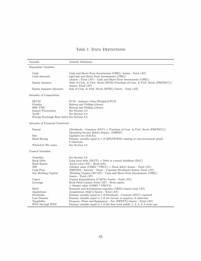
Table 1: Data Definitions

Variable Variable Definition

Dependent Variables

Cash Cash and Short-Term Investments (CHE)/ Assets - Total (AT)Cash alternate log(Cash and Short-Term Investments (CHE)/

(Assets - Total (AT) - Cash and Short-Term Investments (CHE))Equity Issuance (Sale of Com. & Pref. Stock (SSTK)-Purchase of Com. & Pref. Stock (PRSTKC))/

Assets- Total (AT)Equity Issuance alternate Sale of Com. & Pref. Stock (SSTK)/Assets - Total (AT)

Intensity of Competition

EPCM PCM - Industry Value-Weighted PCMFluidity Hoberg and Phillips LibraryHHI TNIC Hoberg and Phillips LibraryImport Penetration See Section 3.3Tariff See Section 3.3Foreign Exchange Rate Index See Section 3.3

Intensity of Financial Constraint

Payout (Dividends - Common (DVC) + Purchase of Com. & Pref. Stock (PRSTKC))/Operating Income Before Deprec. (OIBDP)

Size log(Sales net (SALE))Bond Rating Dummy variable equal to 1 if (SPLTICRM) missing or non-investment grade

0 otherwiseWhited & Wu index See Section 3.4

Control Variables

Volatility See Section 3.2Book Debt Long term debt (DLTT) + Debt in current liabilities (DLC)Book Equity Assets total (AT) - Book debtMB (Market value (CSHO * PRCC) + Book debt)/Assets - Total (AT)Cash Flow (EBITDA - Interest - Taxes - Common Dividend)/Assets- Total (AT)Net Working Captial (Working Capital (WCAP) - Cash and Short-Term Investments (CHE)/

Assets - Total (AT)Capex Capital Expenditures (CAPX)/Assets - Total (AT)Leverage Book Debt/(Assets Total (AT) - Book equity

+ Market value (CSHO * PRCC))R&D Research and development expenses (XRD)/Assets total (AT)Aquisitions Acquisitions (AQC)/Assets - Total (AT)Dividends Dummy variable equal to 1 if Dividends - Common (DVC) reportedLoss Dummy Dummy variable equal to 1 if net income is negative, 0 otherwiseTangibility Property, Plant and Equipment - Net (PPENT)/Assets - Total (AT)IPO1 through IPO5 Dummy variable equal to 1 if the firm went public 1, 2, 3, 4, 5 years ago

45

Tab

le2:

Const

raintTypeCross-C

orrelations

Tab

le2

rep

orts

const

rain

tty

pe

cros

s-co

rrel

atio

ns.

We

use

four

crit

eria

tocl

assi

fyfirm

-yea

rob

serv

atio

ns

asco

nst

rain

ed(C

)or

unco

nst

rain

ed(U

).T

he

sam

ple

isbas

edon

Com

pust

atA

nnual

Indust

rial

file

sov

erth

e19

80-2

007

per

iod.

Payou

tP

olicy

Fir

mS

ize

Bon

dR

ati

ng

WW

ind

ex(C

)(U

)(C

)(U

)(C

)(U

)(C

)(U

)

Payou

tP

olicy

Con

stra

ined

Fir

ms

(C)

45,0

44

Un

con

stra

ined

Fir

ms

(U)

33,0

36

Fir

mS

ize

Con

stra

ined

Fir

ms

(C)

20,1

28

3,3

06

23,4

34

Un

con

stra

ined

Fir

ms

(U)

6,2

80

17,1

54

23,4

34

Bon

dR

ati

ng

Con

stra

ined

Fir

ms

(C)

44,3

15

27,2

79

23,4

28

17,0

98

71,5

94

Un

con

stra

ined

Fir

ms

(U)

729

5,7

57

66,3

36

6,4

86

WW

ind

exC

on

stra

ined

Fir

ms

(C)

20,9

79

2,4

55

19,0

47

35

23,4

32

223,4

34

Un

con

stra

ined

Fir

ms

(U)

4,6

32

18,8

02

110

19,4

39

17,0

40

6,3

94

23,4

34

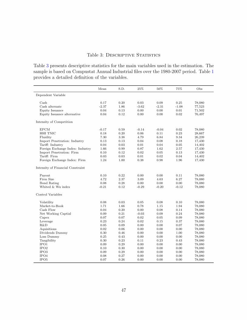
Table 3: Descriptive Statistics

Table 3 presents descriptive statistics for the main variables used in the estimation. Thesample is based on Compustat Annual Industrial files over the 1980-2007 period. Table 1provides a detailed definition of the variables.

Mean S.D. 25% 50% 75% Obs

Dependent Variable

Cash 0.17 0.20 0.03 0.09 0.25 78,080Cash alternate -2.37 1.86 -3.62 -2.31 -1.08 77,523Equity Issuance 0.04 0.13 0.00 0.00 0.01 71,502Equity Issuance alternative 0.04 0.12 0.00 0.00 0.02 76,497

Intensity of Competition

EPCM -0.17 0.59 -0.14 -0.04 0.02 78,080HHI TNIC 0.18 0.20 0.06 0.11 0.23 28,667Fluidity 7.30 3.38 4.79 6.84 9.34 26,239Import Penetration: Industry 0.13 0.13 0.04 0.08 0.18 17,430Tariff: Industry 0.04 0.03 0.01 0.04 0.05 14,402Foreign Exchange Index: Industry 1.66 0.99 0.87 1.62 2.57 17,430Import Penetration: Firm 0.10 0.12 0.02 0.05 0.13 17,430Tariff: Firm 0.03 0.03 0.01 0.02 0.04 14,402Foreign Exchange Index: Firm 1.24 1.00 0.38 0.98 1.96 17,430

Intensity of Financial Constraint

Payout 0.10 0.22 0.00 0.00 0.11 78,080Firm Size 4.72 2.37 3.09 4.63 6.27 78,080Bond Rating 0.08 0.28 0.00 0.00 0.00 78,080Whited & Wu index -0.21 0.12 -0.29 -0.20 -0.12 78,080

Control Variables

Volatility 0.08 0.03 0.05 0.08 0.10 78,080Market-to-Book 1.71 1.66 0.78 1.15 1.94 78,080Cash Flow 0.04 0.20 0.00 0.08 0.14 78,080Net Working Captial 0.09 0.21 -0.03 0.09 0.24 78,080Capex 0.07 0.07 0.02 0.05 0.09 78,080Leverage 0.23 0.24 0.02 0.15 0.37 78,080R&D 0.05 0.09 0.00 0.00 0.07 78,080Aquisitions 0.02 0.06 0.00 0.00 0.00 78,080Dividends Dummy 0.30 0.46 0.00 0.00 1.00 78,080Loss Dummy 0.25 0.43 0.00 0.00 0.00 78,080Tangibility 0.30 0.23 0.11 0.23 0.43 78,080IPO1 0.09 0.29 0.00 0.00 0.00 78,080IPO2 0.10 0.30 0.00 0.00 0.00 78,080IPO3 0.09 0.29 0.00 0.00 0.00 78,080IPO4 0.08 0.27 0.00 0.00 0.00 78,080IPO5 0.07 0.26 0.00 0.00 0.00 78,080

47

Tab

le4:

Cash

holdingsand

Competition

Tab

le4

rep

orts

coeffi

cien

tes

tim

ate

sof

regre

ssio

ns

that

exam

ine

the

effec

tof

com

pet

itio

nan

dfi

nan

cin

gco

nst

rain

tson

cash

hol

din

gs.

Th

esa

mp

leis

bas

edon

Com

pu

stat

An

nu

alIn

du

stri

alfi

les

over

the

1980

-200

7p

erio

d.

Rob

ust

stan

dar

der

rors

are

rep

ort

edu

nd

erth

eco

effici

ents

inp

are

nth

esis

.F

ama-

Mac

Bet

hst

and

ard

erro

rsar

ead

just

edfo

rfi

rst-

ord

erau

toco

rrel

atio

n.

Th

e

sym

bols

***,

**

and

*in

dic

ate

stat

isti

cal

sign

ifica

nce

atth

e1%

,5%

,an

d10

%le

vels

,re

spec

tive

ly.

(1)

(2)

(3)

(4)

(5)

(6)

(7)

(8)

(9)

No

fixed

Fix

edF

am

a-

No

fixed

Fix

edF

am

a-

No

fixed

Fix

edF

am

a-

effec

tseff

ects

MacB

eth

effec

tseff

ects

MacB

eth

effec

tseff

ects

MacB

eth

Com

pet

itio

n:

EP

CM

-0.0

58∗∗∗

-0.0

55∗∗∗

-0.0

44∗∗∗

(0.0

02)

(0.0

02)

(0.0

08)

Com

pet

itio

n:

HH

IT

NIC

-0.1

00∗∗∗

-0.1

17∗∗∗

-0.1

06∗∗∗

(0.0

05)

(0.0

06)

(0.0

10)

Com

pet

itio

n:

Flu

idit

y0.0

09∗∗∗

0.0

11∗∗∗

0.0

09∗∗∗

(0.0

00)

(0.0

00)

(0.0

01)

Siz

e-0

.003∗∗∗

-0.0

06∗∗∗

-0.0

05∗∗∗

-0.0

13∗∗∗

-0.0

18∗∗∗

-0.0

15∗∗∗

-0.0

12∗∗∗

-0.0

17∗∗∗

-0.0

13∗∗∗

(0.0

00)

(0.0

00)

(0.0

01)

(0.0

01)

(0.0

01)

(0.0

02)

(0.0

01)

(0.0

01)

(0.0

02)

Div

iden

d-0

.012∗∗∗

-0.0

08∗∗∗

-0.0

11∗∗

-0.0

21∗∗∗

-0.0

16∗∗∗

-0.0

17∗∗∗

-0.0

13∗∗∗

-0.0

06∗

-0.0

10∗∗

(0.0

01)

(0.0

01)

(0.0

03)

(0.0

02)

(0.0

02)

(0.0

03)

(0.0

02)

(0.0

02)

(0.0

02)

Bon

dR

ati

ng

-0.0

52∗∗∗

-0.0

47∗∗∗

-0.0

35∗∗∗

-0.0

43∗∗∗

-0.0

38∗∗∗

-0.0

39∗∗∗

-0.0

45∗∗∗

-0.0

36∗∗∗

-0.0

44∗∗∗

(0.0

02)

(0.0

02)

(0.0

06)

(0.0

03)

(0.0

03)

(0.0

05)

(0.0

03)

(0.0

03)

(0.0

04)

Vola

tili

ty0.7

15∗∗∗

0.7

83∗∗∗

0.6

60∗∗∗

0.7

51∗∗∗

0.7

82∗∗∗

0.7

46∗∗∗

0.5

95∗∗∗

0.6

05∗∗∗

0.5

86∗∗∗

(0.0

25)

(0.0

32)

(0.0

77)

(0.0

43)

(0.0

56)

(0.1

09)

(0.0

46)

(0.0

60)

(0.1

21)

Mark

et-t

o-B

ook

0.0

12∗∗∗

0.0

11∗∗∗

0.0

11∗∗∗

0.0

14∗∗∗

0.0

14∗∗∗

0.0

17∗∗∗

0.0

13∗∗∗

0.0

12∗∗∗

0.0

14∗∗∗

(0.0

01)

(0.0

01)

(0.0

01)

(0.0

01)

(0.0

01)

(0.0

02)

(0.0

01)

(0.0

01)

(0.0

02)

Cash

flow

0.1

06∗∗∗

0.1

12∗∗∗

0.1

25∗∗∗

0.0

15

0.0

28∗∗∗

0.0

19

0.0

29∗∗∗

0.0

42∗∗∗

0.0

34

(0.0

06)

(0.0

06)

(0.0

12)

(0.0

08)

(0.0

08)

(0.0

17)

(0.0

08)

(0.0

08)

(0.0

16)

Net

work

ing

cap

ital

-0.1

96∗∗∗

-0.1

97∗∗∗

-0.1

80∗∗∗

-0.2

54∗∗∗

-0.2

79∗∗∗

-0.2

40∗∗∗

-0.2

31∗∗∗

-0.2

63∗∗∗

-0.2

22∗∗∗

(0.0

03)

(0.0

04)

(0.0

06)

(0.0

06)

(0.0

08)

(0.0

16)

(0.0

07)

(0.0

08)

(0.0

17)

Cap

ex-0

.453∗∗∗

-0.4

00∗∗∗

-0.4

32∗∗∗

-0.5

94∗∗∗

-0.4

81∗∗∗

-0.5

63∗∗∗

-0.5

80∗∗∗

-0.5

04∗∗∗

-0.5

54∗∗∗

(0.0

08)

(0.0

09)

(0.0

16)

(0.0

16)

(0.0

17)

(0.0

35)

(0.0

17)

(0.0

19)

(0.0

39)

Lev

erage

-0.2

12∗∗∗

-0.2

13∗∗∗

-0.2

08∗∗∗

-0.2

48∗∗∗

-0.2

48∗∗∗

-0.2

37∗∗∗

-0.2

49∗∗∗

-0.2

50∗∗∗

-0.2

44∗∗∗

(0.0

03)

(0.0

03)

(0.0

09)

(0.0

05)

(0.0

05)

(0.0

10)

(0.0

05)

(0.0

05)

(0.0

09)

R&

D0.4

73∗∗∗

0.4

34∗∗∗

0.3

89∗∗∗

0.4

85∗∗∗

0.3

96∗∗∗

0.4

94∗∗∗

0.4

67∗∗∗

0.3

75∗∗∗

0.4

83∗∗∗

(0.0

13)

(0.0

13)

(0.0

30)

(0.0

19)

(0.0

20)

(0.0

47)

(0.0

19)

(0.0

20)

(0.0

49)

Acq

uis

itio

ns

-0.2

65∗∗∗

-0.2

43∗∗∗

-0.2

61∗∗∗

-0.3

47∗∗∗

-0.2

90∗∗∗

-0.3

48∗∗∗

-0.3

69∗∗∗

-0.3

01∗∗∗

-0.3

73∗∗∗

(0.0

08)

(0.0

08)

(0.0

22)

(0.0

13)

(0.0

13)

(0.0

31)

(0.0

13)

(0.0

14)

(0.0

32)

Yea

rfi

xed

effec

tsN

oY

esN

oN

oY

esN

oN

oY

esN

oIn

du

stry

fixed

effec

tsN

oY

esN

oN

oY

esN

oN

oY

esN

oO

bse

rvati

on

s67,1

23

67,1

23

67,1

23

23,5

99

23,5

99

23,5

99

21,4

61

21,4

61

21,4

61

Ad

just

edR

20.4

30.4

40.4

00.5

10.5

30.5

20.5

20.5

40.5

3

48

Tab

le5:

Cash

holdingsand

Competition:Robust

ness

Tab

le5

rep

ort

sco

effici

ent

esti

mat

esof

regr

essi

ons

that

exam

ine

the

effec

tof

com

pet

itio

nan

dfi

nan

cin

gco

nst

rain

tson

cash

hold

ings

.T

he

sam

ple

isb

ase

don

Com

pu

stat

An

nu

alIn

du

stri

alfi

les

over

the

1980

-200

7p

erio

d.

Rob

ust

stan

dar

der

rors

are

rep

orte

du

nd

erth

eco

effici

ents

inp

are

nth

esis

.T

he

sym

bol

s**

*,**

and

*in

dic

ate

stat

isti

cal

sign

ifica

nce

atth

e1%

,5%

,an

d

10%

level

s,re

spec

tive

ly.

(1)

(2)

(3)

(4)

(5)

(6)

(7)

(8)

(9)

Log(C

ash

/A

dd

itio

nal

Bet

wee

nL

og(C

ash

/A

dd

itio

nal

Bet

wee

nL

og(C

ash

/A

dd

itio

nal

Bet

wee

nA

sset

s-C

ash

)C

ontr

ols

regre

ssio

nA

sset

s-C

ash

)C

ontr

ols

regre

ssio

nA

sset

s-C

ash

)C

ontr

ols

regre

ssio

n

Com

pet

itio

n:

EP

CM

-0.2

87∗∗∗

-0.0

54∗∗∗

-0.0

69∗∗∗

(0.0

19)

(0.0

02)

(0.0

03)

Com

pet

itio

n:

HH

IT

NIC

-0.7

10∗∗∗

-0.1

12∗∗∗

-0.1

25∗∗∗

(0.0

55)

(0.0

06)

(0.0

13)

Com

pet

itio

n:

Flu

idit

y0.0

72∗∗∗

0.0

10∗∗∗

0.0

13∗∗∗

(0.0

04)

(0.0

00)

(0.0

01)

Siz

e-0

.005

-0.0

05∗∗∗

0.0

06∗∗∗

-0.0

81∗∗∗

-0.0

16∗∗∗

-0.0

14∗∗∗

-0.0

72∗∗∗

-0.0

16∗∗∗

-0.0

14∗∗∗

(0.0

04)

(0.0

00)

(0.0

01)

(0.0

07)

(0.0

01)

(0.0

02)

(0.0

07)

(0.0

01)

(0.0

02)

Div

iden

d-0

.096∗∗∗

-0.0

05∗∗∗

-0.0

19∗∗∗

-0.1

63∗∗∗

-0.0

11∗∗∗

-0.0

22∗∗

-0.1

05∗∗∗

-0.0

03

-0.0

07

(0.0

15)

(0.0

01)

(0.0

05)

(0.0

26)

(0.0

02)

(0.0

07)

(0.0

28)

(0.0

03)

(0.0

08)

Bon

dra

tin

g-0

.544∗∗∗

-0.0

44∗∗∗

-0.1

03∗∗∗

-0.4

65∗∗∗

-0.0

37∗∗∗

-0.0

55∗∗∗

-0.4

35∗∗∗

-0.0

35∗∗∗

-0.0

56∗∗∗

(0.0

22)

(0.0

02)

(0.0

10)

(0.0

36)

(0.0

03)

(0.0

11)

(0.0

38)

(0.0

03)

(0.0

11)

Vola

tility

7.6

03∗∗∗

0.7

65∗∗∗

0.6

39∗∗∗

8.5

86∗∗∗

0.7

80∗∗∗

0.4

46∗∗∗

7.4

18∗∗∗

0.6

26∗∗∗

0.3

37∗∗∗

(0.3

20)

(0.0

32)

(0.0

61)

(0.5

32)

(0.0

56)

(0.0

92)

(0.5

59)

(0.0

60)

(0.0

94)

Mark

et-t

o-B

ook

0.0

63∗∗∗

0.0

10∗∗∗

0.0

11∗∗∗

0.0

90∗∗∗

0.0

13∗∗∗

0.0

18∗∗∗

0.0

77∗∗∗

0.0

11∗∗∗

0.0

17∗∗∗

(0.0

04)

(0.0

01)

(0.0

01)

(0.0

05)

(0.0

01)

(0.0

02)

(0.0

05)

(0.0

01)

(0.0

02)

Cash

flow

0.7

86∗∗∗

0.1

29∗∗∗

0.1

34∗∗∗

0.2

31∗∗∗

0.0

67∗∗∗

0.0

38∗∗

0.3

17∗∗∗

0.0

69∗∗∗

0.0

59∗∗∗

(0.0

44)

(0.0

07)

(0.0

10)

(0.0

58)

(0.0

10)

(0.0

13)

(0.0

61)

(0.0

11)

(0.0

14)

Net

work

ing

cap

ital

-1.8

09∗∗∗

-0.1

93∗∗∗

-0.2

09∗∗∗

-2.2

92∗∗∗

-0.2

71∗∗∗

-0.2

94∗∗∗

-2.1

46∗∗∗

-0.2

58∗∗∗

-0.2

50∗∗∗

(0.0

40)

(0.0

04)

(0.0

08)

(0.0

68)

(0.0

08)

(0.0

14)

(0.0

72)

(0.0

08)

(0.0

14)

Cap

ex-3

.351∗∗∗

-0.4

15∗∗∗

-0.5

63∗∗∗

-3.4

68∗∗∗

-0.5

01∗∗∗

-0.7

67∗∗∗

-3.5

89∗∗∗

-0.5

17∗∗∗

-0.7

83∗∗∗

(0.0

98)

(0.0

09)

(0.0

23)

(0.1

80)

(0.0

18)

(0.0

39)

(0.1

92)

(0.0

19)

(0.0

40)

Lev

erage

-2.4

61∗∗∗

-0.2

10∗∗∗

-0.2

70∗∗∗

-2.7

89∗∗∗

-0.2

45∗∗∗

-0.3

12∗∗∗

-2.8

00∗∗∗

-0.2

47∗∗∗

-0.3

01∗∗∗

(0.0

32)

(0.0

03)

(0.0

09)

(0.0

57)

(0.0

05)

(0.0

14)

(0.0

60)

(0.0

05)

(0.0

14)

R&

D3.1

57∗∗∗

0.4

36∗∗∗

0.5

76∗∗∗

2.5

70∗∗∗

0.4

01∗∗∗

0.4

90∗∗∗

2.4

63∗∗∗

0.3

82∗∗∗

0.4

03∗∗∗

(0.0

96)

(0.0

13)

(0.0

22)

(0.1

34)

(0.0

19)

(0.0

30)

(0.1

35)

(0.0

20)

(0.0

30)

Acq

uis

itio

ns

-2.5

18∗∗∗

-0.2

55∗∗∗

-0.5

16∗∗∗

-2.7

32∗∗∗

-0.3

05∗∗∗

-0.6

02∗∗∗

-2.8

51∗∗∗

-0.3

12∗∗∗

-0.6

42∗∗∗

(0.1

02)

(0.0

08)

(0.0

38)

(0.1

45)

(0.0

13)

(0.0

48)

(0.1

52)

(0.0

14)

(0.0

48)

Loss

du

mm

y0.0

10∗∗∗

0.0

20∗∗∗

0.0

14∗∗∗

(0.0

02)

(0.0

04)

(0.0

04)

IPO

10.0

32∗∗∗

0.0

61∗∗∗

0.0

36∗∗∗

(0.0

03)

(0.0

07)

(0.0

09)

IPO

20.0

34∗∗∗

0.0

42∗∗∗

0.0

39∗∗∗

(0.0

02)

(0.0

05)

(0.0

06)

IPO

30.0

24∗∗∗

0.0

36∗∗∗

0.0

31∗∗∗

(0.0

02)

(0.0

05)

(0.0

05)

IPO

40.0

15∗∗∗

0.0

18∗∗∗

0.0

12∗

(0.0

02)

(0.0

05)

(0.0

05)

IPO

50.0

13∗∗∗

0.0

14∗∗

0.0

08

(0.0

02)

(0.0

05)

(0.0

05)

Yea

rfi

xed

effec

tsY

esY

esN

oY

esY

esN

oY

esY

esN

oIn

du

stry

fixed

effec

tsY

esY

esN

oY

esY

esN

oY

esY

esN

oO

bse

rvati

on

s66,6

38

67,1

23

67,1

23

23,4

37

23,5

99

23,5

99

21,3

17

21,4

61

21,4

61

Ad

just

edR

20.3

80.4

50.5

50.5

00.5

40.6

00.5

10.5

50.6

1

49

Table 6: Cash holdings and Competition: Sample Splits

Table 6 reports estimates of Competition from a set of estimations of equation (9). The

dependent variable is the cash to assets ratio. The sample is split with respect to the intensity

of financing constraint. We use four criteria to classify firm-year observations as constrained

(C) or unconstrained (U). The sample is based on Compustat Annual Industrial files over the

1980-2007 period. Robust standard errors are reported under the coefficients in parenthesis.

We test for differences in coefficients across equations. The associated p-values are reported in

brackets. The symbols ***, ** and * indicate statistical significance at the 1%, 5%, and 10%

levels, respectively.

Payout Size Rating WW index

EPCMUnconstrainted (U) -0.010 -0.082∗∗∗ -0.066∗∗∗ -0.122∗∗∗

(0.010) (0.008) (0.016) (0.012)

Constrainted (C ) -0.153∗∗∗ -0.150∗∗∗ -0.128∗∗∗ -0.136∗∗∗

(0.005) (0.007) (0.005) (0.006)

(C ) - (U) [0.000] [0.000] [0.000] [0.586]

HHI TNICUnconstrainted (U) -0.062∗∗∗ -0.056∗∗∗ -0.041∗∗∗ -0.057∗∗∗

(0.007) (0.006) (0.009) (0.007)

Constrainted (C ) -0.144∗∗∗ -0.154∗∗∗ -0.122∗∗∗ -0.127∗∗∗

(0.008) (0.013) (0.006) (0.009)

(C ) - (U) [0.000] [0.000] [0.000] [0.006]

FluidityUnconstrainted (U) 0.004∗∗∗ 0.003∗∗∗ 0.001∗ 0.004∗∗∗

(0.001) (0.001) (0.001) (0.001)

Constrainted (C ) 0.014∗∗∗ 0.018∗∗∗ 0.012∗∗∗ 0.015∗∗∗

(0.001) (0.001) (0.000) (0.001)

(C ) - (U) [0.000] [0.000] [0.000] [0.000]

50

Table 7: Cash holdings and Import Penetration

Table 7 presents results of IV regressions of cash holdings on the intensity of competition,

the severity of financing constraints, and control variables. The intensity of competition is

measured by import penetration. Import penetration is instrumented with the level of tariffs

and the foreign exchange rate. The sample is based on Compustat Annual Industrial files over

the 1980-2007 period. Robust standard errors are reported under the estimates in parenthesis.

The symbols ***, ** and * indicate statistical significance at the 1%, 5%, and 10% levels,

respectively.

Second Stage Estimation First Stage Estimation

Cash Cash IP IP(1) (2) (1) (2)

IP: Industry 0.498∗∗∗ Tariff: Industry -0.432∗∗∗

(0.143) (0.071)IP: Firm 0.201∗∗∗ FX rate: Industry 0.014∗∗∗

(0.061) (0.002)Tariff: Firm -0.337∗∗∗

(0.077)FX rate: Firm 0.038∗∗∗

(0.002)

Size -0.014∗∗∗ -0.013∗∗∗ -0.000 -0.002(0.002) (0.002) (0.001) (0.001)

Dividend -0.009∗∗∗ -0.009∗∗∗ 0.005 0.002(0.002) (0.003) (0.005) (0.004)

Bond Rating -0.009 -0.009 -0.001 -0.000(0.005) (0.005) (0.003) (0.003)

Volatility 0.910∗∗∗ 0.778∗∗∗ -0.197 0.027(0.144) (0.139) (0.112) (0.100)

Market-to-Book 0.010∗∗∗ 0.010∗∗∗ -0.000 -0.001∗

(0.002) (0.002) (0.000) (0.001)Cash flow 0.077∗∗∗ 0.075∗∗∗ -0.001 0.006

(0.015) (0.015) (0.004) (0.005)Net working capital -0.138∗∗∗ -0.138∗∗∗ -0.005 -0.015∗

(0.014) (0.014) (0.005) (0.006)Capex -0.236∗∗∗ -0.241∗∗∗ -0.005 0.002

(0.021) (0.021) (0.007) (0.009)Leverage -0.109∗∗∗ -0.109∗∗∗ -0.003 -0.002

(0.009) (0.009) (0.004) (0.005)R&D 0.184∗∗∗ 0.179∗∗∗ -0.024 -0.019

(0.046) (0.046) (0.012) (0.016)Acquisitions -0.141∗∗∗ -0.137∗∗∗ -0.004 -0.012

(0.019) (0.019) (0.007) (0.009)

Year fixed effects Yes Yes Yes YesIndustry fixed effects Yes Yes Yes YesObservations 12,510 12,510 12,510 12,510Adjusted R2 0.33 0.33 0.52 0.53

Hansen J-stat F-test that instruments(p-value) 0.30 0.27 jointly equal zero

(p-value) 0.00 0.00

51

Tab

le8:

EquityIssu

anceand

Competition

Tab

le8

rep

orts

coeffi

cien

tes

tim

ates

of

regr

essi

ons

that

exam

ine

the

effec

tof

com

pet

itio

non

equ

ity

issu

ance

.T

he

sam

ple

isb

ased

on

Com

pu

stat

An

nu

al

Ind

ust

rial

file

sov

erth

e19

80-2

007

per

iod

.R

obu

stst

and

ard

erro

rsar

ere

por

ted

un

der

the

coeffi

cien

tsin

par

enth

esis

.F

am

a-M

acB

eth

stan

dar

der

rors

are

adju

sted

for

firs

t-or

der

auto

corr

elat

ion

.T

he

sym

bol

s**

*,**

an

d*

ind

icat

est

ati

stic

al

sign

ifica

nce

atth

e1%

,5%

,an

d10

%le

vels

,re

spec

tive

ly.

(1)

(2)

(3)

(4)

(5)

(6)

(7)

(8)

(9)

No

fixed

Fix

edF

am

a-

No

fixed

Fix

edF

am

a-

No

fixed

Fix

edF

am

a-

effec

tseff

ects

MacB

eth

effec

tseff

ects

MacB

eth

effec

tseff

ects

MacB

eth

Com

pet

itio

n:

EP

CM

-0.0

20∗∗∗

-0.0

20∗∗∗

-0.0

19∗∗∗

(0.0

02)

(0.0

02)

(0.0

03)

Com

pet

itio

n:

HH

IT

NIC

-0.0

14∗∗∗

-0.0

15∗∗∗

-0.0

15∗∗∗

(0.0

04)

(0.0

04)

(0.0

03)

Com

pet

itio

n:

Flu

idit

y0.0

03∗∗∗

0.0

03∗∗∗

0.0

03∗∗∗

(0.0

00)

(0.0

00)

(0.0

01)

Siz

e-0

.007∗∗∗

-0.0

08∗∗∗

-0.0

07∗∗∗

-0.0

11∗∗∗

-0.0

11∗∗∗

-0.0

11∗∗∗

-0.0

10∗∗∗

-0.0

11∗∗∗

-0.0

11∗∗∗

(0.0

00)

(0.0

00)

(0.0

01)

(0.0

00)

(0.0

00)

(0.0

01)

(0.0

00)

(0.0

00)

(0.0

01)

Cash

flow

-0.0

89∗∗∗

-0.0

92∗∗∗

-0.0

78∗∗∗

-0.1

46∗∗∗

-0.1

47∗∗∗

-0.1

56∗∗∗

-0.1

37∗∗∗

-0.1

37∗∗∗

-0.1

48∗∗∗

(0.0

05)

(0.0

05)

(0.0

13)

(0.0

08)

(0.0

08)

(0.0

17)

(0.0

08)

(0.0

08)

(0.0

17)

Mark

et-t

o-B

ook

0.0

22∗∗∗

0.0

22∗∗∗

0.0

24∗∗∗

0.0

19∗∗∗

0.0

19∗∗∗

0.0

19∗∗∗

0.0

18∗∗∗

0.0

18∗∗∗

0.0

17∗∗∗

(0.0

01)

(0.0

01)

(0.0

02)

(0.0

01)

(0.0

01)

(0.0

01)

(0.0

01)

(0.0

01)

(0.0

01)

Tan

gib

ilit

y0.0

11∗∗∗

0.0

09∗∗

0.0

09∗

0.0

16∗∗∗

0.0

12∗

0.0

17∗∗

0.0

17∗∗∗

0.0

22∗∗∗

0.0

19∗∗

(0.0

02)

(0.0

03)

(0.0

04)

(0.0

04)

(0.0

05)

(0.0

05)

(0.0

04)

(0.0

05)

(0.0

05)

Lev

erage

0.0

03

-0.0

01

0.0

07∗

0.0

09∗∗

0.0

09∗∗

0.0

11

0.0

09∗∗

0.0

09∗

0.0

10

(0.0

02)

(0.0

02)

(0.0

03)

(0.0

03)

(0.0

03)

(0.0

06)

(0.0

03)

(0.0

04)

(0.0

06)

Yea

rfi

xed

effec

tsN

oY

esN

oN

oY

esN

oN

oY

esN

oIn

du

stry

fixed

effec

tsN

oY

esN

oN

oY

esN

oN

oY

esN

oO

bse

rvati

on

s63,0

35

63,0

35

63,0

35

21,1

50

21,1

50

21,1

50

19,2

74

19,2

74

19,2

74

Ad

just

edR

20.1

60.1

70.1

70.1

90.2

00.1

90.2

00.2

00.2

0

52

Tab

le9:

EquityIssu

anceand

Competition:Robust

ness

Tab

le9

rep

ort

sco

effici

ent

esti

mat

esof

regr

essi

ons

that

exam

ine

the

effec

tof

com

pet

itio

non

equ

ity

issu

ance

.T

he

sam

ple

is

bas

edon

Com

pu

stat

An

nu

al

Ind

ust

rial

file

sov

erth

e19

80-2

007

per

iod

.R

obu

stst

and

ard

erro

rsar

ere

por

ted

un

der

the

coeffi

-

cien

tsin

pare

nth

esis

.T

he

sym

bols

***,

**an

d*

ind

icat

est

atis

tica

lsi

gnifi

can

ceat

the

1%,

5%,

and

10%

leve

ls,

resp

ecti

vel

y.

(1)

(2)

(3)

(4)

(5)

(6)

(7)

(8)

(9)

Gro

ssA

dd

itio

nal

Bet

wee

nG

ross

Ad

dit

ion

al

Bet

wee

nG

ross

Ad

dit

ion

al

Bet

wee

nIs

sue

Contr

ols

regre

ssio

nIs

sue

Contr

ols

regre

ssio

nIs

sue

Contr

ols

regre

ssio

n

Com

pet

itio

n:

EP

CM

-0.0

25∗∗∗

-0.0

19∗∗∗

-0.0

15∗∗∗

(0.0

02)

(0.0

02)

(0.0

02)

Com

pet

itio

n:

HH

IT

NIC

-0.0

14∗∗∗

-0.0

14∗∗∗

-0.0

05

(0.0

04)

(0.0

04)

(0.0

08)

Com

pet

itio

n:

Flu

idit

y0.0

03∗∗∗

0.0

03∗∗∗

0.0

03∗∗∗

(0.0

00)

(0.0

00)

(0.0

00)

Siz

e-0

.005∗∗∗

-0.0

08∗∗∗

-0.0

05∗∗∗

-0.0

08∗∗∗

-0.0

11∗∗∗

-0.0

08∗∗∗

-0.0

08∗∗∗

-0.0

11∗∗∗

-0.0

09∗∗∗

(0.0

00)

(0.0

00)

(0.0

01)

(0.0

00)

(0.0

00)

(0.0

01)

(0.0

00)

(0.0

00)

(0.0

01)

Cash

flow

-0.1

26∗∗∗

-0.0

98∗∗∗

-0.1

34∗∗∗

-0.1

81∗∗∗

-0.1

49∗∗∗

-0.1

70∗∗∗

-0.1

73∗∗∗

-0.1

40∗∗∗

-0.1

46∗∗∗

(0.0

05)

(0.0

05)

(0.0

07)

(0.0

07)

(0.0

08)

(0.0

08)

(0.0

08)

(0.0

08)

(0.0

08)

Mark

et-t

o-B

ook

0.0

20∗∗∗

0.0

22∗∗∗

0.0

22∗∗∗

0.0

19∗∗∗

0.0

19∗∗∗

0.0

19∗∗∗

0.0

18∗∗∗

0.0

18∗∗∗

0.0

18∗∗∗

(0.0

01)

(0.0

01)

(0.0

01)

(0.0

01)

(0.0

01)

(0.0

01)

(0.0

01)

(0.0

01)

(0.0

01)

Tan

gib

ilit

y0.0

16∗∗∗

-0.0

13∗∗∗

0.0

11∗

0.0

20∗∗∗

-0.0

10

0.0

20∗∗

0.0

27∗∗∗

0.0

01

0.0

17∗

(0.0

03)

(0.0

03)

(0.0

05)

(0.0

05)

(0.0

06)

(0.0

07)

(0.0

05)

(0.0

06)

(0.0

07)

Lev

erage

-0.0

07∗∗∗

0.0

03

-0.0

13∗

-0.0

10∗∗

0.0

11∗∗∗

0.0

02

-0.0

11∗∗∗

0.0

11∗∗

0.0

07

(0.0

02)

(0.0

02)

(0.0

06)

(0.0

03)

(0.0

03)

(0.0

08)

(0.0

03)

(0.0

04)

(0.0

08)

Cap

ex0.1

34∗∗∗

0.1

30∗∗∗

0.1

20∗∗∗

(0.0

10)

(0.0

20)

(0.0

21)

Acq

uis

itio

ns

0.0

97∗∗∗

0.0

74∗∗∗

0.0

64∗∗∗

(0.0

10)

(0.0

13)

(0.0

13)

,Y

ear

fixed

effec

tsY

esY

esN

oY

esY

esN

oY

esY

esN

oIn

du

stry

fixed

effec

tsY

esY

esN

oY

esY

esN

oY

esY

esN

oO

bse

rvati

on

s67,2

13

63,0

35

63,0

35

23,6

84

21,1

50

21,1

50

21,5

43

19,2

74

19,2

74

Ad

just

edR

20.2

30.1

70.2

80.2

60.2

00.2

90.2

60.2

10.2

9

53

Table 10: Equity Issuance and Competition: Sample Splits

Table 10 reports estimates of Competition from a set of estimations of equation (10). The

dependent variable is equity issuance. The sample is split with respect to the intensity of

financing constraint. We use four criteria to classify firm-year observations as constrained

(C) or unconstrained (U). The sample is based on Compustat Annual Industrial files over the

1980-2007 period. Robust standard errors are reported under the coefficients in parenthesis.

We test for differences in coefficients across equations. The associated p-values are reported in

brackets. The symbols ***, ** and * indicate statistical significance at the 1%, 5%, and 10%

levels, respectively.

Payout Size Rating WW index

EPCMUnconstrainted (U) -0.041∗∗∗ -0.038∗∗∗ -0.023∗ -0.047∗∗∗

(0.009) (0.008) (0.009) (0.012)

Constrainted (C ) -0.064∗∗∗ -0.087∗∗∗ -0.073∗∗∗ -0.088∗∗∗

(0.010) (0.010) (0.011) (0.009)

(C ) - (U) [0.002] [0.000] [0.000] [0.000]

HHI TNICUnconstrainted (U) -0.010∗∗ -0.008∗ -0.009∗ -0.004

(0.004) (0.003) (0.004) (0.003)

Constrainted (C ) -0.015∗ -0.036∗∗∗ -0.018∗∗∗ -0.019∗∗

(0.007) (0.010) (0.005) (0.007)

(C ) - (U) [0.090] [0.002] [0.005] [0.000]

FluidityUnconstrainted (U) 0.002∗∗∗ 0.002∗∗∗ 0.001∗∗∗ 0.002∗∗∗

(0.000) (0.000) (0.000) (0.000)

Constrainted (C ) 0.004∗∗∗ 0.008∗∗∗ 0.004∗∗∗ 0.006∗∗∗

(0.001) (0.001) (0.000) (0.001)

(C ) - (U) [0.016] [0.000] [0.000] [0.000]

54

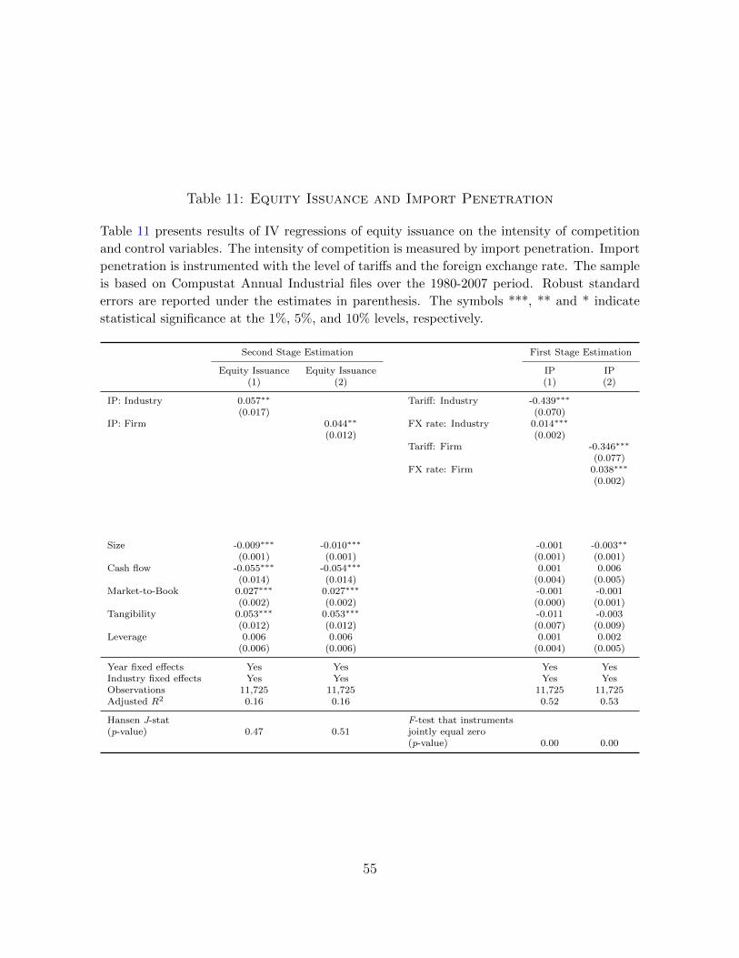
Table 11: Equity Issuance and Import Penetration

Table 11 presents results of IV regressions of equity issuance on the intensity of competition

and control variables. The intensity of competition is measured by import penetration. Import

penetration is instrumented with the level of tariffs and the foreign exchange rate. The sample

is based on Compustat Annual Industrial files over the 1980-2007 period. Robust standard

errors are reported under the estimates in parenthesis. The symbols ***, ** and * indicate

statistical significance at the 1%, 5%, and 10% levels, respectively.

Second Stage Estimation First Stage Estimation

Equity Issuance Equity Issuance IP IP(1) (2) (1) (2)

IP: Industry 0.057∗∗ Tariff: Industry -0.439∗∗∗

(0.017) (0.070)IP: Firm 0.044∗∗ FX rate: Industry 0.014∗∗∗

(0.012) (0.002)Tariff: Firm -0.346∗∗∗

(0.077)FX rate: Firm 0.038∗∗∗

(0.002)

Size -0.009∗∗∗ -0.010∗∗∗ -0.001 -0.003∗∗

(0.001) (0.001) (0.001) (0.001)Cash flow -0.055∗∗∗ -0.054∗∗∗ 0.001 0.006

(0.014) (0.014) (0.004) (0.005)Market-to-Book 0.027∗∗∗ 0.027∗∗∗ -0.001 -0.001

(0.002) (0.002) (0.000) (0.001)Tangibility 0.053∗∗∗ 0.053∗∗∗ -0.011 -0.003

(0.012) (0.012) (0.007) (0.009)Leverage 0.006 0.006 0.001 0.002

(0.006) (0.006) (0.004) (0.005)

Year fixed effects Yes Yes Yes YesIndustry fixed effects Yes Yes Yes YesObservations 11,725 11,725 11,725 11,725Adjusted R2 0.16 0.16 0.52 0.53

Hansen J-stat F-test that instruments(p-value) 0.47 0.51 jointly equal zero

(p-value) 0.00 0.00

55

Tab

le12

:EquityIssu

anceHazard

ModelEst

imates

Tab

le12

rep

ort

ses

tim

ate

sof

pro

port

ion

al

haz

ard

mod

els

for

equ

ity

issu

ance

.A

neq

uit

yis

suan

cesp

ike

occ

urs

ifeq

uit

y

issu

an

ced

eflate

dby

tota

lass

ets

isgr

eate

rth

an3%

,5%

,or

7%.

Th

esa

mp

leis

bas

edon

Com

pu

stat

An

nu

alIn

du

stri

alfi

les

over

the

1980

-200

7p

erio

d.s2

isth

eva

rian

ceof

the

gam

ma

dis

trib

uti

onth

atac

cou

nts

for

un

obse

rved

het

erog

enei

ty.

Sta

nd

ard

erro

rsar

ere

port

edin

pare

nth

esis

.T

he

sym

bol

s**

*,**

and

*in

dic

ate

stat

isti

cal

sign

ifica

nce

atth

e1%

,5%

,an

d10

%le

vel

s,

resp

ecti

vely

.

Issu

an

ceT

hre

shold

:3%

Issu

an

ceT

hre

shold

:5%

Issu

an

ceT

hre

shold

:7%

(1)

(2)

(3)

(4)

(5)

(6)

(7)

(8)

(9)

Com

pet

itio

n:

EP

CM

-0.0

94∗∗∗

-0.0

89∗∗∗

-0.0

68∗∗

(0.0

21)

(0.0

22)

(0.0

24)

Com

pet

itio

n:

HH

IT

NIC

-0.1

78∗

-0.2

26∗

-0.2

28∗

(0.0

83)

(0.0

97)

(0.1

15)

Com

pet

itio

n:

Flu

idit

y0.0

40∗∗∗

0.0

47∗∗∗

0.0

51∗∗∗

(0.0

05)

(0.0

06)

(0.0

07)

Siz

e-0

.036∗∗∗

-0.0

64∗∗∗

-0.0

65∗∗∗

-0.0

79∗∗∗

-0.1

19∗∗∗

-0.1

27∗∗∗

-0.1

01∗∗∗

-0.1

59∗∗∗

-0.1

62∗∗∗

(0.0

06)

(0.0

09)

(0.0

09)

(0.0

07)

(0.0

12)

(0.0

12)

(0.0

08)

(0.0

14)

(0.0

14)

Cash

Flo

w-0

.896∗∗∗

-0.8

02∗∗∗

-0.6

05∗∗∗

-1.0

92∗∗∗

-1.1

43∗∗∗

-0.8

95∗∗∗

-1.1

86∗∗∗

-1.3

00∗∗∗

-1.0

47∗∗∗

(0.0

65)

(0.0

78)

(0.0

83)

(0.0

69)

(0.0

92)

(0.0

98)

(0.0

77)

(0.1

09)

(0.1

15)

Mark

et-t

o-B

ook

0.2

69∗∗∗

0.2

07∗∗∗

0.1

95∗∗∗

0.2

29∗∗∗

0.2

04∗∗∗

0.1

90∗∗∗

0.2

09∗∗∗

0.2

04∗∗∗

0.1

81∗∗∗

(0.0

11)

(0.0

11)

(0.0

11)

(0.0

10)

(0.0

12)

(0.0

12)

(0.0

10)

(0.0

14)

(0.0

14)

Tan

gib

ilit

y-0

.061

-0.0

16

0.0

44

0.1

47∗∗

0.2

16∗

0.2

70∗∗

0.2

52∗∗∗

0.2

77∗

0.3

46∗∗

(0.0

52)

(0.0

79)

(0.0

83)

(0.0

57)

(0.0

93)

(0.0

98)

(0.0

64)

(0.1

10)

(0.1

13)

Lev

erage

-0.4

54∗∗∗

-0.8

09∗∗∗

-0.8

64∗∗∗

-0.2

10∗∗∗

-0.3

41∗∗

-0.3

85∗∗∗

-0.2

27∗∗

-0.1

24

-0.1

64

(0.0

58)

(0.0

98)

(0.1

03)

(0.0

62)

(0.1

11)

(0.1

16)

(0.0

70)

(0.1

28)

(0.1

33)

s20.4

35∗∗∗

0.1

01∗

0.1

10∗

0.2

68∗∗∗

0.1

28∗

0.1

42∗

0.1

71∗

0.1

59∗

0.1

04

(0.0

57)

(0.0

45)

(0.0

49)

(0.0

60)

(0.0

59)

(0.0

65)

(0.0

67)

(0.0

79)

(0.0

79)

Ob

serv

ati

on

s62,7

11

22,1

63

20,2

12

59,8

13

21,3

74

19,5

00

54,9

22

19,8

92

18,1

51

Log-l

ikel

ihood

26,5

57.8

2-9

,707.1

1-8

,981.3

3-2

1,5

01.9

6-7

,703.6

4-7

,057.9

4-1

7,0

82.8

4-6

,008.3

8-5

,476.8

4

56

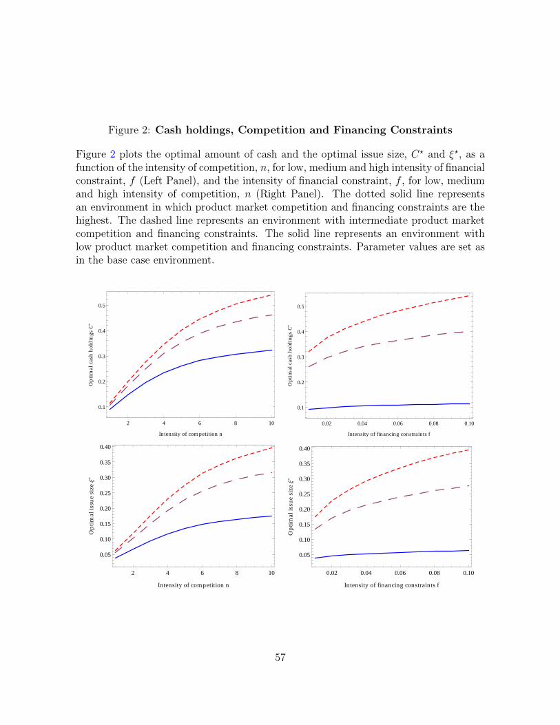
Figure 2: Cash holdings, Competition and Financing Constraints

Figure 2 plots the optimal amount of cash and the optimal issue size, C? and ξ?, as afunction of the intensity of competition, n, for low, medium and high intensity of financialconstraint, f (Left Panel), and the intensity of financial constraint, f , for low, mediumand high intensity of competition, n (Right Panel). The dotted solid line representsan environment in which product market competition and financing constraints are thehighest. The dashed line represents an environment with intermediate product marketcompetition and financing constraints. The solid line represents an environment withlow product market competition and financing constraints. Parameter values are set asin the base case environment.

2 4 6 8 10

0.1

0.2

0.3

0.4

0.5

Intensity of competition n

Op

tim

alcash

hold

ing

sC

*

0.02 0.04 0.06 0.08 0.10

0.1

0.2

0.3

0.4

0.5

Intensity of financing constraints f

Op

tim

alcash

hold

ing

sC

*

2 4 6 8 10

0.05

0.10

0.15

0.20

0.25

0.30

0.35

0.40

Intensity of competition n

Op

tim

alis

su

esiz

eΞ

*

0.02 0.04 0.06 0.08 0.10

0.05

0.10

0.15

0.20

0.25

0.30

0.35

0.40

Intensity of financing constraints f

Op

tim

alis

su

esiz

eΞ

*

57

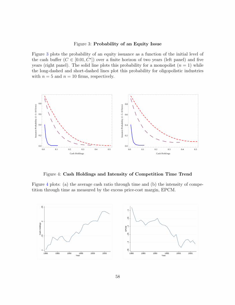
Figure 3: Probability of an Equity Issue

Figure 3 plots the probability of an equity issuance as a function of the initial level ofthe cash buffer (C ∈ [0.01, C?]) over a finite horizon of two years (left panel) and fiveyears (right panel). The solid line plots this probability for a monopolist (n = 1) whilethe long-dashed and short-dashed lines plot this probability for oligopolistic industrieswith n = 5 and n = 10 firms, respectively.

0.0 0.1 0.2 0.3 0.4 0.5

0.0

0.2

0.4

0.6

0.8

Cash Holdings

Issu

an

ce

Prob

ab

ilit

yH1

-5

-10

firm

sL

0.0 0.1 0.2 0.3 0.4 0.5

0.0

0.2

0.4

0.6

0.8

Cash Holdings

Issu

an

ce

Prob

ab

ilit

yH1

-5

-10

firm

sL

Figure 4: Cash Holdings and Intensity of Competition Time Trend

Figure 4 plots: (a) the average cash ratio through time and (b) the intensity of compe-tition through time as measured by the excess price-cost margin, EPCM.

.1.1

5.2

.25

Cas

h H

oldi

ngs

1980 1985 1990 1995 2000 2005 Year

-.35

-.3

-.25

-.2

-.15

-.1

EP

CM

1980 1985 1990 1995 2000 2005 Year

58

competition, cash holdings, and financing decisions - … · competition, cash holdings, and...

Documents