compilation techniques for high-performance...
TRANSCRIPT

Compilation Techniques for High-Performance
Embedded Systems with Multiple Processors
Bjorn Franke
TH
E
U N I V E RS
IT
Y
OF
ED I N B U
RG
H
Doctor of Philosophy
Institute for Computing Systems Architecture
School of Informatics
University of Edinburgh
2004


Abstract
Despite the progress made in developing more advanced compilers for embedded sys-
tems, programming of embedded high-performance computing systems based on Dig-
ital Signal Processors (DSPs) is still a highly skilled manual task. This is true for
single-processor systems, and even more for embedded systems based on multiple
DSPs. Compilers often fail to optimise existing DSP codes written in C due to the
employed programming style. Parallelisation is hampered by the complex multiple ad-
dress space memory architecture, which can be found in most commercial multi-DSP
configurations.
This thesis develops an integrated optimisation and parallelisation strategy that can
deal with low-level C codes and produces optimised parallel code for a homogeneous
multi-DSP architecture with distributed physical memory and multiple logical address
spaces. In a first step, low-level programming idioms are identified and recovered. This
enables the application of high-level code and data transformations well-known in the
field of scientific computing. Iterative feedback-driven search for “good” transforma-
tion sequences is being investigated. A novel approach to parallelisation based on a
unified data and loop transformation framework is presented and evaluated. Perfor-
mance optimisation is achieved through exploitation of data locality on the one hand,
and utilisation of DSP-specific architectural features such as Direct Memory Access
(DMA) transfers on the other hand.
The proposed methodology is evaluated against two benchmark suites (DSPstone
& UTDSP) and four different high-performance DSPs, one of which is part of a com-
mercial four processor multi-DSP board also used for evaluation. Experiments confirm
the effectiveness of the program recovery techniques as enablers of high-level trans-
formations and automatic parallelisation. Source-to-source transformations of DSP
codes yield an average speedup of 2.21 across four different DSP architectures. The
parallelisation scheme is – in conjunction with a set of locality optimisations – able to
produce linear and even super-linear speedups on a number of relevant DSP kernels
and applications.
iii

Declaration
I declare that this thesis was composed by myself, that the work contained herein is
my own except where explicitly stated otherwise in the text, and that this work has not
been submitted for any other degree or professional qualification except as specified.
(Bjorn Franke)
iv

Table of Contents
1 Introduction 1
1.1 High Performance Embedded Systems . . . . . . . . . . . . . . . . . 1
1.2 High Performance Digital Signal Processing . . . . . . . . . . . . . . 1
1.2.1 Parallelism in DSP Applications . . . . . . . . . . . . . . . . 3
1.2.2 Parallelism in DSP Architectures . . . . . . . . . . . . . . . . 4
1.3 Goals of this Thesis . . . . . . . . . . . . . . . . . . . . . . . . . . . 6
1.3.1 Contributions . . . . . . . . . . . . . . . . . . . . . . . . . . 7
1.4 Overview . . . . . . . . . . . . . . . . . . . . . . . . . . . . . . . . 8
2 Background 9
2.1 Digital Signal Processing . . . . . . . . . . . . . . . . . . . . . . . . 9
2.1.1 Applications . . . . . . . . . . . . . . . . . . . . . . . . . . 10
2.1.2 Algorithms . . . . . . . . . . . . . . . . . . . . . . . . . . . 11
2.1.3 Systems . . . . . . . . . . . . . . . . . . . . . . . . . . . . . 13
2.2 Embedded Processors . . . . . . . . . . . . . . . . . . . . . . . . . . 15
2.2.1 DSPs and Multimedia processors . . . . . . . . . . . . . . . 16
2.2.2 Memory System . . . . . . . . . . . . . . . . . . . . . . . . 16
2.2.3 Parallel DSP Architectures . . . . . . . . . . . . . . . . . . . 19
2.3 Data and Loop Transformations . . . . . . . . . . . . . . . . . . . . 22
2.3.1 Definitions . . . . . . . . . . . . . . . . . . . . . . . . . . . 22
2.3.2 Loop Transformations . . . . . . . . . . . . . . . . . . . . . 27
2.3.3 Data Transformations . . . . . . . . . . . . . . . . . . . . . . 30
2.4 Parallelisation . . . . . . . . . . . . . . . . . . . . . . . . . . . . . . 31
v

2.4.1 Parallelism in DSP Codes . . . . . . . . . . . . . . . . . . . 32
2.4.2 Definitions . . . . . . . . . . . . . . . . . . . . . . . . . . . 32
2.4.3 Instruction-Level Parallelism . . . . . . . . . . . . . . . . . . 33
2.4.4 Loop-Level Parallelism . . . . . . . . . . . . . . . . . . . . . 34
2.4.5 Task-Level Parallelism . . . . . . . . . . . . . . . . . . . . . 35
2.4.6 Parallelism Detection . . . . . . . . . . . . . . . . . . . . . . 36
2.4.7 Parallelism Exploitation . . . . . . . . . . . . . . . . . . . . 37
2.4.8 Locality Optimisations . . . . . . . . . . . . . . . . . . . . . 37
2.5 Summary . . . . . . . . . . . . . . . . . . . . . . . . . . . . . . . . 38
3 Infrastructure 39
3.1 DSP Benchmarks . . . . . . . . . . . . . . . . . . . . . . . . . . . . 39
3.1.1 DSPstone . . . . . . . . . . . . . . . . . . . . . . . . . . . . 39
3.1.2 UTDSP . . . . . . . . . . . . . . . . . . . . . . . . . . . . . 40
3.1.3 MediaBench . . . . . . . . . . . . . . . . . . . . . . . . . . 40
3.2 Digital Signal Processors . . . . . . . . . . . . . . . . . . . . . . . . 43
3.2.1 Analog Devices ADSP-21160 (SHARC) . . . . . . . . . . . 43
3.2.2 Analog Devices TS-101S (TigerSHARC) . . . . . . . . . . . 46
3.2.3 Philips TriMedia TM-1300 . . . . . . . . . . . . . . . . . . . 51
3.2.4 Texas Instruments TMS320C6201 . . . . . . . . . . . . . . . 52
3.3 Data and Loop Transformations . . . . . . . . . . . . . . . . . . . . 54
3.3.1 Unified Transformation Framework . . . . . . . . . . . . . . 55
3.4 Summary . . . . . . . . . . . . . . . . . . . . . . . . . . . . . . . . 58
4 Related Work 59
4.1 Program Recovery . . . . . . . . . . . . . . . . . . . . . . . . . . . 59
4.1.1 Balasa et al. (1994) . . . . . . . . . . . . . . . . . . . . . . . 59
4.1.2 Held and Kienhuis (1995) . . . . . . . . . . . . . . . . . . . 60
4.1.3 van Engelen and Gallivan (2001) . . . . . . . . . . . . . . . . 61
4.2 High-Level Transformations for DSP Codes . . . . . . . . . . . . . . 61
4.2.1 Su et al. (1999) . . . . . . . . . . . . . . . . . . . . . . . . . 61
4.2.2 Gupta et al. (2000) . . . . . . . . . . . . . . . . . . . . . . . 62
vi

4.2.3 Qian et al. (2002) . . . . . . . . . . . . . . . . . . . . . . . . 62
4.2.4 Falk et al. (2003) . . . . . . . . . . . . . . . . . . . . . . . . 62
4.2.5 Kulkarni et al. (2003) . . . . . . . . . . . . . . . . . . . . . . 63
4.3 Parallelisation of DSP Codes . . . . . . . . . . . . . . . . . . . . . . 64
4.3.1 Teich and Thiele (1991) . . . . . . . . . . . . . . . . . . . . 64
4.3.2 Kim (1991) . . . . . . . . . . . . . . . . . . . . . . . . . . . 65
4.3.3 Hoang and Rabaey (1992) . . . . . . . . . . . . . . . . . . . 66
4.3.4 Koch (1995) . . . . . . . . . . . . . . . . . . . . . . . . . . 67
4.3.5 Newburn and Shen (1996) . . . . . . . . . . . . . . . . . . . 67
4.3.6 Ancourt et al. (1997) . . . . . . . . . . . . . . . . . . . . . . 68
4.3.7 Karkowski and Corporaal (1998) . . . . . . . . . . . . . . . . 68
4.3.8 Wittenburg et al. (1998) . . . . . . . . . . . . . . . . . . . . 69
4.3.9 Kalavade et al. (1999) . . . . . . . . . . . . . . . . . . . . . 70
4.4 Summary . . . . . . . . . . . . . . . . . . . . . . . . . . . . . . . . 70
5 Program Recovery 73
5.1 Pointer Conversion . . . . . . . . . . . . . . . . . . . . . . . . . . . 74
5.1.1 Motivation . . . . . . . . . . . . . . . . . . . . . . . . . . . 75
5.1.2 Program Representation . . . . . . . . . . . . . . . . . . . . 77
5.1.3 Other Definitions . . . . . . . . . . . . . . . . . . . . . . . . 77
5.1.4 Assumptions and Restrictions . . . . . . . . . . . . . . . . . 79
5.1.5 Pointer Analysis Algorithm . . . . . . . . . . . . . . . . . . 84
5.1.6 Pointer Conversion Algorithm . . . . . . . . . . . . . . . . . 90
5.1.7 Example . . . . . . . . . . . . . . . . . . . . . . . . . . . . 91
5.2 Modulo Removal . . . . . . . . . . . . . . . . . . . . . . . . . . . . 94
5.2.1 Motivation . . . . . . . . . . . . . . . . . . . . . . . . . . . 94
5.2.2 Notation . . . . . . . . . . . . . . . . . . . . . . . . . . . . 95
5.2.3 Assumptions and Restrictions . . . . . . . . . . . . . . . . . 97
5.2.4 Modulo Removal Algorithm . . . . . . . . . . . . . . . . . . 97
5.2.5 Example . . . . . . . . . . . . . . . . . . . . . . . . . . . . 100
5.3 Running Example . . . . . . . . . . . . . . . . . . . . . . . . . . . . 105
5.3.1 Pointer Conversion . . . . . . . . . . . . . . . . . . . . . . . 106
vii

5.3.2 Modulo Removal . . . . . . . . . . . . . . . . . . . . . . . . 107
5.4 Summary . . . . . . . . . . . . . . . . . . . . . . . . . . . . . . . . 108
6 High-Level Transformations for Single-DSP Performance Optimisation 111
6.1 Introduction . . . . . . . . . . . . . . . . . . . . . . . . . . . . . . . 112
6.2 Motivation . . . . . . . . . . . . . . . . . . . . . . . . . . . . . . . . 114
6.3 High-Level Transformations . . . . . . . . . . . . . . . . . . . . . . 115
6.4 Example . . . . . . . . . . . . . . . . . . . . . . . . . . . . . . . . . 116
6.5 Transformation-oriented Evaluation . . . . . . . . . . . . . . . . . . 118
6.5.1 Pointer Conversion . . . . . . . . . . . . . . . . . . . . . . . 118
6.5.2 Unrolling . . . . . . . . . . . . . . . . . . . . . . . . . . . . 120
6.5.3 SIMD vectorisation . . . . . . . . . . . . . . . . . . . . . . . 124
6.5.4 Delinearisation . . . . . . . . . . . . . . . . . . . . . . . . . 124
6.5.5 Array padding . . . . . . . . . . . . . . . . . . . . . . . . . 127
6.5.6 Loop Tiling . . . . . . . . . . . . . . . . . . . . . . . . . . . 127
6.5.7 Scalar Replacement . . . . . . . . . . . . . . . . . . . . . . . 128
6.5.8 Summary . . . . . . . . . . . . . . . . . . . . . . . . . . . . 128
6.6 Iterative Search . . . . . . . . . . . . . . . . . . . . . . . . . . . . . 129
6.6.1 Iterative Optimisation Framework . . . . . . . . . . . . . . . 129
6.6.2 Iterative Search Algorithm . . . . . . . . . . . . . . . . . . . 130
6.7 Results and Analysis . . . . . . . . . . . . . . . . . . . . . . . . . . 132
6.7.1 Benchmark-oriented Evaluation . . . . . . . . . . . . . . . . 132
6.7.2 Architecture-oriented Evaluation . . . . . . . . . . . . . . . . 141
6.8 Related Work and Discussion . . . . . . . . . . . . . . . . . . . . . . 142
6.9 Conclusion . . . . . . . . . . . . . . . . . . . . . . . . . . . . . . . 144
7 Parallelisation for Multi-DSP 145
7.1 Motivation & Example . . . . . . . . . . . . . . . . . . . . . . . . . 146
7.1.1 Memory Model . . . . . . . . . . . . . . . . . . . . . . . . . 146
7.1.2 Example . . . . . . . . . . . . . . . . . . . . . . . . . . . . 147
7.2 Parallelisation . . . . . . . . . . . . . . . . . . . . . . . . . . . . . . 150
7.3 Partitioning and Mapping . . . . . . . . . . . . . . . . . . . . . . . . 150
viii

7.3.1 Notation . . . . . . . . . . . . . . . . . . . . . . . . . . . . 151
7.3.2 Partitioning . . . . . . . . . . . . . . . . . . . . . . . . . . . 152
7.3.3 Mapping . . . . . . . . . . . . . . . . . . . . . . . . . . . . 153
7.3.4 Algorithm . . . . . . . . . . . . . . . . . . . . . . . . . . . . 154
7.4 Address Resolution . . . . . . . . . . . . . . . . . . . . . . . . . . . 157
7.4.1 Algorithm . . . . . . . . . . . . . . . . . . . . . . . . . . . . 157
7.4.2 Synchronisation . . . . . . . . . . . . . . . . . . . . . . . . 158
7.5 Example . . . . . . . . . . . . . . . . . . . . . . . . . . . . . . . . . 158
7.5.1 Sequential program . . . . . . . . . . . . . . . . . . . . . . . 159
7.5.2 Partitioning . . . . . . . . . . . . . . . . . . . . . . . . . . . 159
7.5.3 Mapping . . . . . . . . . . . . . . . . . . . . . . . . . . . . 162
7.5.4 Address Resolution . . . . . . . . . . . . . . . . . . . . . . . 168
7.5.5 Modulo Removal . . . . . . . . . . . . . . . . . . . . . . . . 170
7.6 Related Work . . . . . . . . . . . . . . . . . . . . . . . . . . . . . . 172
7.7 Conclusion . . . . . . . . . . . . . . . . . . . . . . . . . . . . . . . 173
8 Localisation and Bulk Data Transfers 175
8.1 Motivation . . . . . . . . . . . . . . . . . . . . . . . . . . . . . . . . 176
8.2 Access Separation . . . . . . . . . . . . . . . . . . . . . . . . . . . . 181
8.2.1 Standard Approach . . . . . . . . . . . . . . . . . . . . . . . 181
8.2.2 Access Separation Based on Explicit Processor IDs . . . . . . 185
8.3 Local Access Optimisations . . . . . . . . . . . . . . . . . . . . . . 188
8.4 Remote Access Vectorisation . . . . . . . . . . . . . . . . . . . . . . 189
8.4.1 Load Loops . . . . . . . . . . . . . . . . . . . . . . . . . . . 189
8.4.2 Access Vectorisation . . . . . . . . . . . . . . . . . . . . . . 191
8.5 Example . . . . . . . . . . . . . . . . . . . . . . . . . . . . . . . . . 194
8.6 Empirical Results . . . . . . . . . . . . . . . . . . . . . . . . . . . . 200
8.6.1 Parallelism Detection . . . . . . . . . . . . . . . . . . . . . . 200
8.6.2 Partitioning and Address Resolution . . . . . . . . . . . . . . 202
8.6.3 Localisation . . . . . . . . . . . . . . . . . . . . . . . . . . . 203
8.7 Related Work . . . . . . . . . . . . . . . . . . . . . . . . . . . . . . 204
8.8 Conclusion . . . . . . . . . . . . . . . . . . . . . . . . . . . . . . . 206
ix

9 Future Work 207
9.1 High-Level Transformations . . . . . . . . . . . . . . . . . . . . . . 207
9.1.1 Transformation Selection based on Machine Learning . . . . 207
9.2 Communication Optimisation . . . . . . . . . . . . . . . . . . . . . . 208
9.2.1 Computation/Communication Pipelining . . . . . . . . . . . 208
9.2.2 Advanced DMA Modes . . . . . . . . . . . . . . . . . . . . 210
9.3 Extended Parallelisation . . . . . . . . . . . . . . . . . . . . . . . . 210
9.3.1 Exploitation of Task-Level Parallelism . . . . . . . . . . . . . 210
9.3.2 Iterative Parallelisation . . . . . . . . . . . . . . . . . . . . . 211
9.3.3 Combined Parallelisation and Single-Processor Optimisation . 212
9.4 Design Space Exploration . . . . . . . . . . . . . . . . . . . . . . . . 213
10 Conclusion 215
10.1 Contributions . . . . . . . . . . . . . . . . . . . . . . . . . . . . . . 215
10.1.1 Program Recovery . . . . . . . . . . . . . . . . . . . . . . . 215
10.1.2 High-Level Transformations for Single-Processor
Performance Optimisation . . . . . . . . . . . . . . . . . . . 216
10.1.3 Parallelisation for Multi-DSP . . . . . . . . . . . . . . . . . 217
10.1.4 Localisation and Bulk Data Transfers . . . . . . . . . . . . . 217
10.2 Conclusions . . . . . . . . . . . . . . . . . . . . . . . . . . . . . . . 218
A Refereed Conference and Journal Papers 221
B Fully ANSI C compliant example codes 223
Bibliography 225
x

Nomenclature
I S Set of iteration spaces
P Set of all programs
SP Sequential program
T Set oftransformations
T P Parallel target program
T S Set of space-time mappings
U Array access matrix
A Array index constraint matrix
B Iteration space constraint matrix
Idm m-dimensional identity matrix
L Generalised linearisation matrix
Ln1 Linearisation matrix
S Generalised strip-mine matrix
Sn1 Strip-mine matrix
TS Transformation matrix
U Unimodular matrix
xi

X Transformation matrix
aaa Array bounds vector
bbb Size vector
III,KKK Vectors of loop iterators
JJJ Array index vector
uuu Vector of constant offsets of an affine array reference
fn Flow function for node n
H(i) Alignment measure for index i
ik Loop iterator at level k
IN[n] Dataflow set at entry of node n
jk Array index at level k
L Dataflow lattice
LBk Lower bound at level k
OUT [n] Dataflow set at exit of node n
p Program
PG Code generation function
TA Adaptor transformations
TE Enabler transformations
TP Performer transformations
UBk Upper bound at level k
xii

Chapter 1
Introduction
1.1 High Performance Embedded Systems
High Performance Computing is not the exclusive domain of computational science.
Instead, high computational power is required in many devices, which are not built
with the primary goal of providing their users with a computer of any kind, but to
offer a service in which a powerful computer plays a central role. Medical imaging
is an example of the application of such a High Performance Embedded System. As
signals from an X-ray or magneto-resonance device come in at a very high rate, they
are processed by a computer to provide the radiologist with a visualisation suitable for
further diagnosis. Other examples include radar and sonar processing, speech synthesis
and recognition, and a broad range of applications in the fields of multimedia and
telecommunications.
In this thesis, embedded systems based on Digital Signal Processors (DSPs) are
investigated as one specific example of the many different system configurations in
use today. Real-time digital signal processing requires high-performance processors
due to the strict timing constraints imposed by the volatile nature of signals.
1.2 High Performance Digital Signal Processing
Digital Signal Processors (DSPs) are ubiquitous and increasingly important in the
1

2 Chapter 1. Introduction
telecommunications and electronics industry. The industry’s demand for short time-
to-market, high computational performance, low power consumption and flexibility
over the lifespan of their devices – e.g. to adapt to new standards, to add new fea-
tures or to correct bugs of earlier versions – make programmable DSPs the favourite
choice for many new electronic designs. For example, the business magazine EETimes
reports of impressive growth rates forecasts over the next three years:
EETimes (www.eetimes.com)(By Mark LaPedus, Semiconductor Business News, June 11, 2003 (7:01 p.m. ET)
DSPs also remain a sizzling market. This business is forecast to rise 27.7percent to $6.2 billion in 2003, 20.8 percent in 2004 to $7.5 billion, 21.0percent to $9.1 billion in 2005, and 6.0 percent to $9.6 billion in 2006.
From the constraints set by the DSP application domain arise some (partially mutu-
ally exclusive) requirements for signal processors distinct to those of general purpose
processors. DSPs have to be able to deliver enough computational power to cope
with demanding applications like image and video processing whilst meeting further
constraints such as low cost and low power. As a result, DSPs are usually highly spe-
cialised and adapted to their specific application domain, but notoriously difficult to
program.
DSPs find application in a broad range of different signal processing environments,
which are characterised by their algorithm complexity and predominant sampling rates.
An overview of these properties for different applications is given in figure 1.1.
DSP applications have sampling rates that vary by more than twelve orders of mag-
nitude (Glossner et al., 2000). Weather forecasting on the lower end of the frequency
scale has sampling rates of about 1/1000Hz, but utilises highly complex algorithms,
while demanding radar applications require sampling rates over a gigahertz, but ap-
ply relatively simple algorithms. Both extremes have in common that they rely on
high-performance computing systems, possibly based on DSPs, to meet the timing
constraints imposed on them. With the current state of processor technology, it is still
not possible to deliver the required compute power for some applications with just a
single DSP, but the combined power of several DSPs is needed. Unfortunately, such
multi-DSP systems are even more difficult to program than a single DSP.

1.2. High Performance Digital Signal Processing 3
Figure 1.1: DSP application complexity and sampling rates (Jinturkar, 2000)
1.2.1 Parallelism in DSP Applications
DSP and multimedia algorithms are often highly repetitive as incoming data streams
are uniformly processed. This regularity suggests that DSP and multimedia applica-
tions contain higher levels of parallelism than general purpose applications, possibly
at different granularities. Figure 1.2 shows the inherent parallelism of three classes of
workloads (general purpose, DSP, video). DSP and video codes contain larger amounts
of exploitable parallelism than general purpose codes, with video codes containing the
most parallelism. This fact not only simplifies the work of automatically parallelising
compilers, but more importantly it provides the basis for larger performance benefits
according to Amdahl’s Law. While general purpose codes can only experience theo-
retical speedups of up to 10 due to parallel execution, DSP and multimedia codes are
subject to more than an order of magnitude higher performance improvements.
In the past, DSP software was mainly composed of small kernels and software de-
velopment in assembly language was acceptable. Similar to other fields of computing,

4 Chapter 1. Introduction
Figure 1.2: Potential parallel speedup of different workloads (Jinturkar, 2000)
code complexity in the DSP area began to increase and application development using
high-level languages such as C became the norm. Recent DSP applications require ten
thousand or more lines of C code (Glossner et al., 2000).
Problems exploiting the parallelism in DSP codes arise from this use of C as the
dominating high-level language for DSP programming. C is particularly difficult to
analyse due to the large degrees of freedom given to the programmer. Even worse, C
permits a low-level, hardware-oriented programming style that is frequently used by
embedded systems programmers to manually tune their codes for better performance.
Without accurate analyses, however, success in detection and exploitation of program
parallelism is very limited. Against this background, optimising as well as parallelising
compilers must find a way to cope with idiosyncracies of the C programming language
and the predominant programming style in order to be successful.
1.2.2 Parallelism in DSP Architectures
DSP manufacturers’ response to the increased demand for computational power of
their devices was the adoption of the Very Large Instruction Word (VLIW) paradigm

1.2. High Performance Digital Signal Processing 5
Figure 1.3: Application performance requirements (Glossner et al., 2000)
to offer larger amounts of Instruction-Level Parallelism (ILP) in their processors. This
approach is very appealing as improved semiconductor manufacturing technology al-
lows for the integration of more functional units on the same chip whilst maintaining
the same sequential high-level programming model. However, it presents the compil-
ers for these architectures with the problems of identifying simultaneously executable
instructions and of constructing compact and efficient schedules.
Figure 1.3 shows the performance requirements of typical DSP applications. While
for most current end-user telecommunication applications a single DSP suffices, more
compute-intensive applications in the telecommunication infrastructure, multimedia
and speech processing domains require more computer power than an individual DSP
can deliver. To accommodate these demanding applications, provisions to combine in-
dividual DSPs to a multi-DSP were taken by their manufacturers. Nevertheless, mul-
tiprocessor capabilities of most commercial DSPs are very restricted due to cost when
compared with larger mainstream parallel computer systems. Again, manufacturers
follow their design philosophy to implement only the most frequently utilised func-

6 Chapter 1. Introduction
tionality in hardware. This minimal hardware support has significant consequences for
the design of parallel DSP software. Writing parallel code for a multi-DSP target is
still a highly skilled, manual task with associated costs due to person power, increased
time-to-market and reduced reliability.
1.3 Goals of this Thesis
This thesis aims to identify and eliminate some of the obstacles to compiler-based op-
timisation and parallelisation of real-world DSP codes written in C. The choice of C
as the input language is motivated by its wide-spread use in the DSP world. While
other languages might be more suitable for compiler analysis and transformation, they
lack the support of the DSP community. Heavily used idioms and constructs in exist-
ing DSP codes that defeat program analysis and transformation are identified. Based
on this, automatable program recovery techniques that reconstruct a more compiler-
friendly form from the original sources are developed. Later work in transforming and
parallelising DSP codes will rely on the success of this stage.
High-level transformations successful in the optimisation of scientific codes have
found little consideration in the DSP domain. Instead, embedded systems compiler
research has primarily focused on low-level techniques such as register allocation
and instruction selection to accommodate the unconventional and specialised micro-
architectures found in typical DSPs. As compilers become more mature, improvements
in low-level transformations deliver diminishing returns. In this thesis, the effective-
ness of a set of high-level source-to-source transformations well-known from other
areas of high-performance computing is evaluated in the context of compilation for
single DSPs. Starting with the hypothesis that the application of high-level transfor-
mations should significantly improve performance, while finding a “good” sequence
of transformations to achieve this goal is hard, a feedback-driven iterative approach to
performance optimisation is investigated.
Parallelisation of DSP applications is still in its infancy, despite the progress in au-
tomatic parallelisation in the last two decades (Banerjee et al., 1993). This is partly
due to the complexities of the C programming language, but can also be attributed to

1.3. Goals of this Thesis 7
the idiosyncracies of the DSP target processors. Unconventional memory models and
little hardware support for multiprocessing complicate parallelisation. Rather than ab-
stract away these details and develop parallelisation techniques on more conventional
Symmetric Multiprocessing (SMP) architectures, a commercially available, yet in its
features representative, multi-DSP platform was chosen to ensure real-world relevance
of this work. In this thesis, a methodology for the parallelisation of DSP codes is devel-
oped that takes into account the specific properties of existing multi-DSP architectures
and the C programming language.
Data locality is one of the key contributors to high performance. DSP specific
features such as a higher bandwidth to on-chip memory than to off-chip memory are
analysed to determine how they affect program performance under the aspect of data
locality. Mechanisms to exploit data locality and to integrate them into an overall
parallelisation strategy are developed.
1.3.1 Contributions
This thesis provides contributions to several relevant aspects in compiler-based DSP
code optimisation and parallelisation. The main achievements are in the following
fields:
• Program Recovery
Identification and elimination of frequently used idioms defeating program anal-
ysis and transformation.
• Single Processor Performance Optimisation
Evaluation of high-level code and data transformations embedded in an iterative
compilation framework against two important DSP benchmark suites and four
DSP architectures.
• Automatic Parallelisation
Development of a novel transformation enabling efficient parallelisation on mul-
tiple address space hardware whilst maintaining a single address space program-
ming model suitable for further single-processor optimisation.
8 Chapter 1. Introduction
• Locality Optimisations
Performance optimisation through exploitation of data locality and DSP-specific
hardware features.
1.4 Overview
This thesis is structured as follows. In chapter 2 background information on digital sig-
nal processing, embedded processors, data and loop transformations and program par-
allelism is provided. Chapter 3 presents more background information on the specific
infrastructure, i.e. benchmarks, architectures and program transformation frameworks,
used in this thesis. Related work is discussed in chapter 4. Two program recovery tech-
niques used later in this thesis are developed in chapter 5. An evaluation of high-level
transformations for single-processor performance improvement is contained in chapter
6. Parallelisation of DSP codes is the subject of chapter 7, before locality optimisa-
tions are presented in chapter 8. An outlook to future work is given in chapter 9, before
chapter 10 summarises and concludes.

Chapter 2
Background
This chapter presents background material in the areas of digital signal processing and
compiler optimisations, and is structured as follows. In section 2.1 a short introduction
to digital signal processing is given. This is followed by an overview of architectural
features of digital signal processors in section 2.2. Data and loop transformations are
the subjects of section 2.3, and, finally, parallelisation is covered in section 2.4.
2.1 Digital Signal Processing
Limitations of analogue signal processing operations and the rapid progress made in
the field of Very Large Scale Integration (VLSI) led to the development of techniques
for Digital Signal Processing (DSP). To enable DSP, an analogue signal is sampled
at regular intervals and each of the sample values is represented as a binary number,
which is then further processed by a digital computer (often in the form of a specialised
Digital Signal Processor (DSP)). In general, the following sequence of operations is
commonly found in DSP systems (Mulgrew et al., 1999):
• Sampling and Analogue-to-Digital (A/D) conversion.
• Mathematical processing of the digital information data stream.
• Digital-to-Analogue (D/A) conversion and filtering.
Among the many attractions of DSP the most important factors are:
• High achievable (and extendable) accuracy.
9

10 Chapter 2. Background
• Good repeatability.
• Insensitivity to noise.
• High processing speed.
• High flexibility.
• Realisation of complex operations (Linear phase filters, Fourier trans-form, matrix manipulations).
• Low manufacturing cost.
• Low power consumption.
• Low maintenance cost.
Usually, not all of these benefits can be realised simultaneously, i.e. they are par-
tially mutually exclusive. For example, extending the dynamic range (e.g. by use of
floating-point arithmetic) can have adverse effects on cost, processing speed and power
consumption. However, this and other disadvantages are often not severe and for many
system designers DSP technology is regularly the preferred choice for approaching
their specific task.
The following sections briefly present an overview of the wide spectrum of DSP
applications, and give a short introduction to signal representation, DSP algorithms and
their characteristics. This is followed by a presentation of DSP systems, in particular
digital signal processors, and their architectural features.
2.1.1 Applications
Digital signal processing is not a technique restricted to specific applications, but can
be found in very different application areas. Its application domain spans from the
ubiquitous GSM mobile phone with modest signal processing requirements to highly
compute-intensive radar signal generation and analysis. According to Mulgrew et al.
(1999) the generic DSP application areas are:
• Speech and Audionoise reduction (Dolby), coding, compression (MPEG), recognition, speechsynthesis.
• Musicrecording, playback and mixing, synthesis of digital music, CD players.

2.1. Digital Signal Processing 11
• Telephonyspeech, data and video transmission by wire, radio or optical fibre.
• Radiodigital modulators and modems for cellular telephony.
• Signal analysisspectrum estimation, parameters estimation, signal modelling and classifi-cation.
• Instrumentationsignal generation, filtering, signal parameter measurement.
• Image processing2-D filtering, enhancement, coding, compression, pattern recognition.
• Multimediageneration, storage and transmission of sound, motion pictures, digital TV,HDTV, DVD, MPEG, video conferencing, satellite TV.
• Radarfiltering, target detection, position and velocity estimation, tracking, imag-ing, direction finding, identification.
• Sonaras for radar but also for use in acoustic media such as sea.
• Controlservomechanisms, automatic pilots, chemical plant control.
• Biomedicalanalysis, diagnosis, patient monitoring, preventive health care, telemedicine.
• Transportvehicle control (braking, engine management) and vehicle speed measure-ment.
• Navigationaccurate position determination, global positioning, map display.
2.1.2 Algorithms
There are several textbooks on the subject of DSP algorithms (e.g. Mulgrew et al.,
1999; Smith, 1997; Proakis and Manolakis, 1995). From a compiler writer’s point
of view, it is not necessary to understand how these algorithms work. However, it is
important to know and to understand the characteristics of the algorithms and their
concrete implementations. These are the inputs supplied to a compiler, and affect the
ability of the compiler to generate efficient code.

12 Chapter 2. Background
The following two sections present the important characteristics of many DSP pro-
grams and their impact on the design of specialised digital signal processors.
2.1.2.1 Properties
The list below presents the most important characteristics of DSP algorithms relevant
to a compiler.
• Streaming Data
Most DSP algorithms exclusively access current data, i.e. data within a small spatial
neighbourhood progressing in time. Once the data has been processed and output, no
further references to it will take place.
• Sums of Products
Digital filters, for example, are frequently stated as sums of products, i.e. two vectors
are multiplied pairwise and then the products are accumulated to form a single number
as a result.
• Constant Iteration Count
As data is often processed in constant sized blocks, many loops have constant iteration
counts that do not depend on any result computed in the loop body.
• Data Independent Control Flow
Many DSP algorithms show very little if any variation in control flow. Often control
flow is only dependent on the size of the input, but not on the actual input values.
• Linear Array Traversals
Data access patterns are mainly linear, i.e. array index functions are affine. The most
prominent exception to this is the ubiquitous Fast Fourier Transform (FFT). This algo-
rithm shows highly non-linear data access patterns.
2.1.2.2 Architectural Implications
The previously listed properties of the most important DSP algorithms have affected
the design of highly adapted digital processors aimed at digital signal processing.

2.1. Digital Signal Processing 13
These Digital Signal Processors (DSP) are discussed later in this chapter in more de-
tail. At this point, only a brief overview of how DSP algorithms influence the design
of DSPs is given.
The high frequency at which multiply-accumulate operations are found in many
DSP algorithms has led to the integration of highly efficient Multiply-Accumulate
(MAC) instructions in the instruction set of almost all DSPs. MAC operations typi-
cally take two operands and accumulate the result of their multiplication in a dedicated
processor register. Thereby, sums of products can be implemented using very few, fast
instructions.
Further improvements come from Zero-overhead loops (ZOLs). A loop counter
can be initialised to a constant value which then determines how often the following
loop body is executed. This eliminates the need for potentially stalling conditional
branches in the implementation of loops with fixed iteration counts.
Streaming data as the main domain of DSP shows very little temporal locality. This
and the real-time guarantees required from many DSP systems make data caches un-
favourable. Instead, fast and deterministic on-chip memories are the preferred design
option.
Memory in DSPs is usually banked. Two independent memory banks and internal
buses allow for the simultaneous fetch of two operands as required by many arithmetic
operations, e.g. MAC.
Address computation is supported by Address Generation Units (AGUs), which
operate in parallel to the main data path. Thus, the data path is fully available for user
calculations and does not need to perform auxiliary computations.
2.1.3 Systems
In embedded systems processors usually work under tighter constraints than in a desk-
top environment. This is particularly true for DSPs, which are often faced with real-
time performance requirements on top of other system constraints.
DSP system engineering is not the issue of this thesis. However, it is important to
understand the main system requirements to avoid solutions that are feasible on their
own, but do not fit into the overall system design. For example, compiler transfor-

14 Chapter 2. Background
mations that blow up code size to such an extent that it does not fit into the restricted
on-chip memories differentiate embedded compiler construction from general-purpose
compilers where code size is less critical.
In the following section a short overview of DSP system requirements and the DSP
software design and implementation process are given.
2.1.3.1 System Requirements
DSPs often operate in highly specialised systems and must meet the systems’ over-
all constraints. The main requirements of DSP-based systems are summarised in the
following list.
• Real-Time (high bandwidth, low latency)
Most DSP systems work under real-time constraints, i.e. data must be processed at an
externally defined rate.
• Memory (deterministic, high bandwidth)
Memory access times must be deterministic in order to be able to reason about worst
case behaviour. This and high memory bandwidth is important to guarantee real-time
performance.
• Power/Energy (battery powered devices, cooling)
As many DSPs are embedded in battery powered devices with restricted battery capacity,
low energy consumption is paramount. Low power dissipation is a further requirement
originating from the need for passive processor cooling in embedded systems.
• Cost (Development/Manufacturing)
DSPs find use in large volume products as well as small scale applications, e.g. pro-
totypes. Both markets demand low cost solutions. However, for volume products the
manufacturing cost dominates the overall cost, whereas development cost dominates the
low volume domain.
• Time-to-Market
DSPs are a driving force behind many new technologies for which time-to-market is crit-

2.2. Embedded Processors 15
ical. Programmability in high-level programming languages, e.g. C, and high efficiency
of the compiler-generated code are important to reduce product development cycles.
• Physical size (Embedded)
Due to their embedded nature, DSPs must not take up too much space.
Of these, real-time performance, efficiency of memory accesses, low power and
development cost and time-to-market are important to compiler construction.
2.1.3.2 Software Design and Implementation
The DSP software design process has the peculiar property of being split into two
separate high-level and low-level stages. On the high level, simple algorithms are for-
mulated by means of equations which form basic blocks for the construction of more
complex algorithms. These high-level formulations are translated into Synchronous
Data Flow (SDF) Graphs (Lee, 1995) and implemented in high-level languages like
Matlab (Rijpkema et al., 1999). Due to performance reasons, proven high-level imple-
mentations are re-implemented on a lower level using programming languages like C
or C++ enhanced with system specific and non-standard features. Where performance
is still not sufficient, assembly is used to optimise performance bottlenecks.
In this work, the lower level of abstraction is considered. Programmers are pro-
vided with an optimising and parallelising C compiler, which saves him from manually
tuning and parallelising code for a specific target architecture.
2.2 Embedded Processors
The requirements of a processor powering a desktop computer and a processor embed-
ded in a device designed for one fixed application differ significantly. Depending on
the requirements to that specific device certain constraints such as performance, cost,
size, energy consumption and power dissipation must be met. Consequently, manufac-
turers have developed specialised processor architectures for different user profiles and
requirements. In this section an overview of embedded digital signal and multimedia
processors is presented.

16 Chapter 2. Background
2.2.1 DSPs and Multimedia processors
Leupers (2000) indentifies five classes of embedded processors: Microcontrollers,
RISC processors, Digital Signal Processors (DSPs), Multimedia processors and Ap-
plication Specific Instruction Set Processors (ASIPs). Of these five classes, only DSPs
and multimedia processors are of interest as the targeted application domain covers
DSP and multimedia workloads. According to Leupers (2000) DSPs are characterised
by special hardware to support digital filter and Fast Fourier Transform (FFT) imple-
mentation, a certain degree of instruction-level parallelism, special-purpose registers
and special arithmetic modes. Multimedia processors, on the other hand, are specially
adapted to the higher demands of video and audio processing in that they follow the
VLIW paradigm for statically scheduling parallel operations. To achieve a higher re-
source utilisation multimedia processors often offer SIMD instructions and conditional
instructions for the fast execution of if-then-else statements.
However, manufacturers have not generally adopted this classification and tend
to classify and name their products by the type of applications found in the market
they are aiming at. In particular, manufacturers refer to their processors aiming at
multimedia processing as DSPs, too. We adhere to the manufacturers’ classification
(DSP/multimedia processor) of their processors.
In the following two paragraphs the generic features of the memory systems found
in DSPs as well as frequently implemented approaches to parallel DSP architectures
are discussed. After that, four specific DSPs used as vehicles for experimentation in
this study are introduced and explained in more detail.
2.2.2 Memory System
Digital signal processors as specialised processor architectures have a memory system
which significantly differs from those found in general-purpose processors and com-
puting systems. In the following paragraph the main differences and idiosyncracies as
relevant to the rest of this thesis are briefly sketched.

2.2. Embedded Processors 17
2.2.2.1 On-Chip and Off-Chip Memory Banks
Most embedded DSPs comprise of several kilobytes of fast on-chip SRAM. This is due
to the fact that SRAM integrated on the same chip as the core processor allows for fast
access without wait states. Thus, processor performance is not impeded by the memory
system. Furthermore, on-chip SRAM allows for the construction of inexpensive and
compact DSP systems with a minimal number of external components.
Usually, a DSP’s internal memory is banked, i.e. distributed over several memory
banks, thereby allowing for parallel accesses. The reason for this physical memory
organisation comes from the fact that many operations in DSP applications require
two or sometimes three operands to compute a single result. Fetching these operands
sequentially leads to poor resource utilisation as the processor might have to wait until
all operands become available before it can resume computation. Parallel accesses
to operands are a way of matching processor and memory speed by providing higher
memory bandwidth. Hence, appropriate assignment of program variables to memory
banks is crucial to achieve good performance.
The on-chip storage capacity is not always sufficient to hold a program’s code and
data. In such a case, external memory can be connected to a DSP through an external
memory interface. Often the latency of external memory is higher than that of the
on-chip SRAM as a cheaper, but slower memory technology might be used (lower
cost and improved memory density). Additionally, bandwidth to external memory is
usually smaller as parallel internal buses are multiplexed onto a single external bus
(smaller pin count) operating at a slower clock rate (simpler board design, cheaper
external components). Avoiding excessive numbers of external memory accesses by
appropriate program/data allocation and utilisation of on-chip memory together with
the exploitation of efficient data transfer modes (e.g. Direct Memory Access (DMA))
are necessary to save program performance from severe degradation.
2.2.2.2 Address Generation Units
Many DSPs provide dedicated Address Generation Units (AGUs) (also known as Data
Address Generators (DAGs)) for parallel next-address computations (Leupers and Mar-
wedel, 1996). As these AGUs are not part of the data path and perform their compu-

18 Chapter 2. Background
tations simultaneously to it, instruction-level parallelism is increased. Auto-increment
addressing modes make the use of the AGUs explicit in the program code. Generation
of efficient addressing code is subject of e.g. Leupers and Marwedel (1996); Leupers
(2003).
Figure 2.1: Address generation unit of the SHARC 2106x DSP (Smith, 2000)
Figure 2.1 shows the address generation units of the Analog Devices SHARC
2106x DSP. Two separate units DAG1 and DAG2 are dedicated to data (DM) and
program (PM) memory, respectively. This allows for the simultaneous and indepen-
dent address computation for accesses to the two memory banks. Each unit contains
four banks of eight registers (length registers L, base registers B, index registers I, and
modify registers M).
DSP algorithms frequently traverse linear arrays. For the purpose of addressing
contiguous elements of such an array, an index register Ix is used to point to the current
element. An auto-increment access automatically updates the value in Ix so that it
points to the next element afterwards. To accomplish this, the element size as stored in
a modify register My is added to the current address in Ix. The result is stored back to
Ix.

2.2. Embedded Processors 19
Circular buffers as an algorithmic basis for digital filters are also directly supported
by the AGU. A length register Lx and a base register By contain the length and the start
address such that the necessary wrap-around is automatically performed by a modulo
unit when required.
Additional circuitry for bit-reversed addressing is available. This exotic address-
ing mode is mainly used in the efficient implementation of the FFT. However, most
compilers are not able to exploit this specific feature.
2.2.2.3 Direct Memory Access
Many DSP applications process streaming data at a very high throughput rate. In
order to keep up with the required I/O bandwidth, DSPs typically employ sophisticated
controllers for independently managing I/O and memory accesses.
Such a controller capable of reading and writing to or from memory without CPU
intervention is known as a Direct Memory Access (DMA) controller (Tanenbaum, 1999).
Once a DMA transfer has been initiated, the CPU can continue until it receives an in-
terrupt indicating the completion of the data transfer.
Using DMA for bulk data transfers between internal and external memory or be-
tween internal memories of different processors greatly improves the efficiency of
memory accesses for two reasons: First, bulk data transfers are faster than many in-
dividual transfers as the transfer setup costs (bus request and arbitration, etc.) are
incurred only once. Second, the CPU can continue normal operations and perform
useful work while the data transfer is in progress.
2.2.3 Parallel DSP Architectures
As technology limits the maximal clock rate and the application limits the available
instruction-level parallelism, the performance of a single DSP cannot be increased
arbitrarily. However, certain applications (e.g. radar/sonar processing) require more
compute power than a single DSP can deliver. The solution to this problem is to employ
multiple DSPs and let them co-operate on a common task under the assumption that
this task can be decomposed into sub-tasks which then can be approached by different

20 Chapter 2. Background
processors in parallel. Thus, it seems likely to experience a shorter processing time
and to meet the requirements a single processor could not fulfil.
Partitioning the original task into sub-tasks and mapping these onto a parallel tar-
get architecture generally requires some communication between the processors as the
sub-tasks are seldomly independent of each other. As the mode of inter-processor com-
munications depends on the logical memory organisation of the parallel computer, the
two dominating paradigms shared memory and distributed memory are briefly intro-
duced in the following paragraph and discussed in the context of their implications on
how processors communicate.
2.2.3.1 Inter-processor Communication
Inter-processor communication and memory organisation are intimately related as data
is transferred from the scope of one processor to another. Furthermore, logical and
physical memory organisation must be distinguished.
Common logical address space organisations are single address space and multiple
private address spaces. In the first programming paradigm, each program has the same
uniform view of the memory space and can access data arbitrarily. Communication is
performed via writing to and reading from this shared memory. In a multiple private
address space environment, each program maintains its own address space. Processes
communicate by explicitly sending and receiving data.
Physical memory organisation in existing computers can have many different forms.
Depending on whether a single physical address space is maintained, or multiple pri-
vate address spaces are provided, parallel computers can be classified as Shared Mem-
ory and Distributed Memory computers. However, this classification can be mislead-
ing as shared memory computers (i.e. with a single address space) are often based on
physically distributed memory banks.
Clearly, the logical address space must be mapped onto the physical memory or-
ganisation. This can be done either explicitly, i.e. under the control of the programmer,
or implicitly, i.e. by some extra layer of hardware or software. From a programmer’s
point of view the implicit model is preferable, because it saves one from explicit data
management. Performance, however, can suffer if the implementation of the address

2.2. Embedded Processors 21
space mapping is not very well tuned.
2.2.3.1.1 Distributed Memory In this approach to logical memory organisation,
each process maintains its own private address space, i.e. each process owns some
memory which no other process is able to address and, thus, to access. Frequently, the
physical memory organisation matches the logical organisation with each processor
having private, local memory attached.
Communication in-between processes is managed by explicitly introducing Send
and Receive instructions into the code, which initiate messages to be send from one
process to another. On the hardware side, these messages are passed via a communi-
cations network spanning the processors.
Parallel computers following the distributed memory paradigm are often consid-
ered to be more scalable as memory is not a single resource which can potentially be-
come a bottleneck. Furthermore, distributed memory computers are less cost-intensive
as no additional hardware creating a single address space is required. However, due to
the need for explicit Message Passing, programming in the distributed memory model
can be difficult and prone to errors.
2.2.3.1.2 Shared Memory This approach to logical memory organisation offers the
programmer a single address space, i.e. no matter where data is stored all processes can
access it using the same address. To prevent memory from becoming a bottleneck, the
physical implementation of the shared memory paradigm is often based on physically
distributed memory and additional circuitry to maintain a uniform address space.
Processes communicate by writing values to memory, which can then be read by
other processes. For the programmer, there is no distinction in-between local and
remote memory. With respect to performance, however, locality is an important issue
as accesses to local data are usually much faster than remote accesses.
Shared memory computers are less scalable due to the need to maintain a single
address space. Additional hardware or software can form a bottleneck and limit the
overall performance. However, from a programmer’s point of view shared memory
computers are preferable as the single address space makes programming much easier.

22 Chapter 2. Background
2.2.3.1.3 Hybrid Memory Organisation As the driving design philosophy of the
DSP domain is to keep hardware cheap, small and fast, existing DSP architectures
are either representatives of the distributed memory paradigm or some hybrid forms
with restricted shared memory support. Concrete examples of such architectures are
presented and discussed in the chapter 3.2.
2.3 Data and Loop Transformations
Restructuring a (possibly sequential) program can greatly improve its performance on a
single processor or enable its efficient execution on multiple processors. Restructuring
mainly focuses on program loops and data layout as DSP performance is dominated
by these structures.
Fundamental definitions are presented in the next section. Section 2.3.2 presents an
overview of loop transformations. Data transformations are discussed in section 2.3.3.
2.3.1 Definitions
To enable formal and systematic program restructuring, a formalism to describe pro-
gram loops, data declarations and accesses and also the transformations themselves is
required. In this section well-established algebraic representations for loop nests, array
declarations and different loop and data transformations are presented. These will be
used throughout this thesis.
2.3.1.1 Loop Nest Representation
Figure 2.2 shows a loop nest of depth n. Each of the loops is normalised, i.e. has unit
stride. To obtain unit stride for all loops of a given loop nest, loop normalisation can
be applied. After that, each loop iterates through a sequence of consecutive integer
numbers. The Iteration Space of a normalised loop nest is an ordered set of loop
iterations, in which each iteration is represented by the current values of the iterators
i1, . . . , in of the loops surrounding the loop body.
The loop iterators can be represented by a column vector III = [i1, . . . , in]T where

2.3. Data and Loop Transformations 23
for (i1 = LB1 ; i1 <= UB1 ; i1++) {
for (i2 = LB2(i1) ; i2 <= UB2(i1); i2++) {
· · ·
for (in = LBn(i1, . . . , in−1) ; i1 <= UBn(i1, . . . , in−1); in++)
· · ·
· · ·
}
}
Figure 2.2: Loop nest of depth n
[i1, . . . , in] denotes the transpose of the vector III. The loop ranges are then defined by
the following system of inequalities:
LB1 ≤ i1 ≤UB1 (2.1)
LB2(i1)≤ i2 ≤UB2(i1)...
LBn(i1, . . . , in−1)≤ in ≤UBn(i1, . . . , in−1)
Usually, the loop bounds LBk and UBk are restricted to affine expressions. With
this assumption of loop bound linearity, the Iteration Space of the loop nest is a finite
convex polyhedron in Zn. For convenience, this polyhedron is represented as
BIII ≤ bbb (2.2)
where B ∈ Z2n×n is called the iteration space constraint matrix, III the vector of loop
iterators ik,∀k ∈ 1, . . . ,n and bbb ∈ Z2n the constant size vector.
2.3.1.2 Data Representation
Formalising data layout transformations requires an algebraic description of the shape
of data, in particular arrays. This is achieved in a similar way as for loops. Array

24 Chapter 2. Background
bounds are described by a system of inequalities, which form a polyhedral Array Index
Space.
An m-dimensional array a[LB1 . . .UB1][LB2 . . .UB2] . . . [LBm . . .UBm] is described
by following system of inequalities
LB1 ≤ j1 ≤UB1 (2.3)
LB2 ≤ j2 ≤UB2...
LBm ≤ jm ≤UBm
Rewriting these inequalities in matrix representation, the Array Index Space is also
characterised by the polyhedral AJJJ ≤ aaa , where JJJ represents the array indices, and aaa
the array bounds. Often, arrays are assumed to be allocated statically, i.e. the array
bounds LBk and UBk are constant. In this case the array index space is rectangular.
2.3.1.3 Unimodular Transformations
Many different reordering transformations have been studied (Bacon et al., 1994) and
each of them has its own legality checks and transformation rules. To overcome this
difficulty, a unified framework of unimodular transformations based on unimodular
matrices has been suggested. It is able to describe transformations obtained from com-
bining loop interchange, loop skewing and loop reversal.
Unimodular transformations are unimodular linear mappings from one iteration
space into another. Thus, each transformation can be described as a unimodular matrix
and the application of a transformation corresponds to the multiplication of an index
vector by such a matrix.
Definitions of unimodular transformations and matrices are given, before a number
of important properties are listed. This section is based on the material in Banerjee
(1991, 1993) with some references also to Barnett and Lengauer (1992) and Yiyun
et al. (1998).
Definition 2.1 (Unimodularity) A transformation is unimodular if and only if
1. it is invertible,

2.3. Data and Loop Transformations 25
2. it maps integer points to integer points, and
3. its inverse maps integer points to integer points.
An integer matrix is unimodular if and only if it has a unit determinant.
From this definition a number of useful properties can be derived:
Property 2.1 (Combination) If U1,U2 are unimodular matrices, U = U1U2 is still a
unimodular matrix.
Property 2.2 (Inversion) If U is a unimodular matrix, its inverse U−1 is still a uni-
modular matrix.
Property 2.3 (Preservation) If a unimodular transformation is applied to a unit stride
normalised multi-nested loop, this loop keeps its normalisation and stride.
Property 2.4 (Decomposition) If U is a unimodular matrix, there exists a sequence
of fundamental unimodular matrices U1, . . . ,UT such that U = U1 . . .UT .
Property 2.5 (Fundamental Unimodular Matrices) A column-skewing matrix V can
be replaced by the multiple of a row-skewing matrix U and two interchange matri-
ces T1,T2: V = T1UT2. Therefore fundamental unimodular matrices include row-
skewing, interchange and reversal matrices.
The application of a unimodular transformation yields a correct program as long
as dependence relations are preserved, i.e. the lexicographical order of dependent
iterations is preserved in the new iteration space.
Unimodular transformations can be easily integrated into a transformation frame-
work (Wolf and Lam, 1991) and greatly simplify code generation as long as the appro-
priate unimodular transformation matrix can be found. However, unimodular transfor-
mations have certain shortcomings, too. It is difficult to apply them to non-perfectly
nested loops, and they cannot represent some important transformations like loop fu-
sion, loop distribution and statement reordering.

26 Chapter 2. Background
2.3.1.4 Non-Unimodular Transformations
Resigning from unimodularity opens the field for a large class of new transformations.
However, non-unimodular transformations can introduce non-unit loop strides and,
more serious than that, non-convex boundaries.
Kelly and Pugh (1993) have developed a unifying reordering framework that ad-
dresses this problem and incorporates unimodular and non-unimodular transforma-
tions such as loop interchange, distribution, skewing, index set splitting and statement
reordering.
The key concept in the paper of Kelly and Pugh (1993) is to introduce Schedules to
represent transformations. A schedule is a mapping from the original iteration space
into the new iterations space and has the following form
T : [i1, . . . , im]→ [ f1, . . . , fn]|C (2.4)
where the iteration variables i1, . . . , im represent the loop nest around the statement,
the f js are functions of the iteration variables, and C is an optional restriction on the
domain of schedules.
Schedules can be used to express unimodular transformations. This is the case
when all statements are mapped using the same schedule, the f js are linear functions
of the iteration variables, the schedule is invertible and unimodular, the old and the new
iteration space have the same dimensions and no further restrictions C to the domain
apply.
Relaxing these restrictions on schedules enables the representation of a broader
class of reordering transformations. The proposed generalisation includes the follow-
ing points: a separate schedule for each statement, a symbolic constant term in the f js,
invertible, but not necessarily unimodular schedules, different dimensionality of old
and new iteration space, piece-wise schedules, and inclusion of integer division and
modular operations (with constant denominators) in the f js.
Using this generalisation, transformations constructed from the following set of
fundamental transformations can be represented: loop interchange, loop reversal, loop
skewing, statement reordering, loop distribution, loop fusion, loop alignment, loop
interleaving, loop blocking, index set splitting, loop coalescing and loop scaling.

2.3. Data and Loop Transformations 27
Specific examples and further information on the construction and use of schedules
can be found in Kelly and Pugh (1993).
2.3.2 Loop Transformations
Concentrating program restructuring on the most frequently executed and thus most
profitable to optimise program segments leads immediately to Loop Transformations.
The objectives for transforming a loop can vary. They include improving locality by
changing a loop’s data access pattern, increasing parallelism on a certain loop level by
iteration reordering, minimising the size of the sequential loop level, improving load
balance and supporting or enabling later compiler stages by conditioning a loop in a
given way.
Loop transformation generally targets Fortran-style DO loops as they can be appro-
priately modelled using linear algebra. WHILE loops do not fit easily into this model,
because generally the iteration condition cannot be determined at compile-time.
2.3.2.1 Array Reference Representation
Most formalisms to describe array references are restricted to affine index functions.
Non-affine index expressions are beyond the scope of linear algebra and require more
advanced formalisms. The vast majority of array indices, however, are affine (Paek
et al., 2002).
An access to an m-dimensional array has the form a[ j1][ j2] . . . [ jm]. In an affine
model, each of the indices jk is determined by a function fk of the form
fk(i1, . . . , in) = ak,1× i1 +ak,2× i2 + . . .ak,n× in + ck (2.5)
where all ak,l and ck are constant. Thus, the entire access can be written as
UIII +uuu (2.6)
where U is an integer matrix and uuu is a vector.

28 Chapter 2. Background
2.3.2.2 Unimodular Loop Transformations
Unimodular loop transformations can be represented using an algebraic framework
based on unimodular matrices. Throughout this paragraph we follow the example of
Kulkarni and Stumm (1993) in the presentation of unimodular loop transformations.
Before any loop transformation is applied its legality is tested (Wolf and Lam,
1991). Legal transformations do not change the result that is produced by a loop, in
particular, dependent iterations must be executed in their lexicographic order.
A unimodular loop transformation is represented by a unimodular matrix U . This
matrix U maps an iteration vector III = [i1, . . . , in]T into a new iteration vector KKK =
[k1, . . . ,kn]T :
UIII = KKK (2.7)
Application of a loop transformation involves the computation of new array index
expressions and loop bounds. For the computation of the new index expressions, the
iterator III in the index function UIII +uuu is replaced by III = U−1KKK according to equation
2.7. Thus, the new index expression has the form:
UU−1KKK +uuu (2.8)
Determining the new loop bounds involves computing affine functions specifying
the convex polyhedron resulting from transforming the original iteration space BIII ≤ bbb.
Applying the identity transformation U−1U the iteration space can be rewritten as
BU−1
UIII ≤ bbb (2.9)
Using equation (2.7) gives
BU−1KKK ≤ bbb (2.10)
If B ′ = BU−1 is lower triangular, the new loop bounds can be directly obtained
from the rows of B ′. In general, Fourier-Motzkin variable elimination (Schrijver, 1986)
has to be applied on B′ to obtain the new bounds. This approach works well for loops
of any dimension as long as the original loop bounds are constant (Kumar et al., 1991),
but becomes more complex when the original loop bounds are linear.
2.3. Data and Loop Transformations 29
Avoiding these complications in determining the new loop bounds, equation 2.10
can be further transformed into
XBU−1KKK ≤ Xbbb, where X =
[
U 0
0 U
]
(2.11)
The new loop bounds are now of the form
B′KKK ≤ bbb′′′, where B
′ = XBU−1 and bbb′′′ = Xbbb (2.12)
2.3.2.3 List of Loop Transformations
Covering loop transformations in an algebraic or any other framework is not sufficient.
The most challenging problem remains to find a “good” sequence of loop transforma-
tions. Identifying a sequence of legal transformations that help exploit architectural
features of the hardware involves searching a potentially huge search space.
The following list contains some of the most important (not exclusively unimodu-
lar) loop transformations together with a short description of their potential usage. This
list is far from complete, but it reflects the broad field of applications in parallelisation,
locality optimisation, and other purposes.
Loop interchange exchanges two loop levels. This can expose parallelism at the inner
level enabling vectorisation or it can expose parallelism at the outer level.
Wavefront restructures a loop to execute sets of independent iterations. The new loop
construct comprises a sequential outer loop, and a parallel inner loop. Loop
skewing is one well-known instance of wavefront transformation.
Loop tiling divides the iteration space into smaller blocks, which are subsequently
iterated individually. This aims at increasing locality within the tiles and helps
to efficiently utilise data caches by reusing cached data.
Loop strip-mining splits a linear loop into an inner and an outer loop such that the
inner loop iterates over strips of fixed size and the outer loop enumerates the
individual strips. This transformation is traditionally used to match the size of a
vectorisable loop with the vector register size.

30 Chapter 2. Background
Loop unrolling duplicates the loop body a given number of times, and updates the in-
dex variable within these copies and the loop step accordingly. Due to the larger
number in the newly created loop body the scheduler has more flexibility and
can possibly construct a more efficient schedule. Furthermore, loop overhead is
reduced by loop unrolling.
More formal background on loop transformations can be found in e.g. Kulkarni
and Stumm (1993), and Bacon et al. (1994) comprises an extensive list of loop trans-
formations.
2.3.3 Data Transformations
Program performance is not only affected by its loop structure, but also data organisa-
tion plays an equally important role. Cost of data accesses are usually not uniform, i.e.
the time required to fetch data from memory depends on the location the data is stored
in. In computers with hierarchical memory organisation, data stored “closer” to a pro-
cessor can be accessed faster than remote data. Moving frequently accessed data closer
to the processor where it is processed, should thus increase overall performance. Data
Transformations aim at rearranging the data layout so as to minimise the overhead due
to access latency. This task is non-trivial as data access patterns often put incompatible
constraints on the relative data placement and distribution across processors.
Most DSP programs operate heavily on data stored in arrays. Therefore, the focus
of this work is on the reorganisation of array structures. For this, techniques from the
field of scientific computing are employed as codes from both domains have similar
properties.
While some data transformations can be expressed using unimodular transforma-
tions, most data transformations are highly specialised and require their own transfor-
mation framework. Therefore, no detailed description of unimodular data transforma-
tions is given. Specific examples can be found in e.g. Bacon et al. (1994) and Kulkarni
and Stumm (1993).
2.4. Parallelisation 31
2.3.3.1 List of Data Transformations
A large number of data transformations have been developed and have come to appli-
cation in modern compilers. A short list of some of the most important data transfor-
mations is given below.
Alignment aims to improve the relative placement of array elements of different ar-
rays. Array alignment reduces communication overhead as array elements are
placed on the same processor.
Data Distribution maps the array index space onto the processor space, i.e. an array
is distributed across a number of processors. When accesses to local memory are
significantly faster than to remote memory, data distribution can help improve
performance by minimising the number of remote references.
Delinearisation is the transformation of a linear array into an array with higher dimen-
sionality. Although the immediate benefits of this transformation are marginal,
it enables or supports further transformations such as the aforementioned data
distribution.
Padding inserts dummy elements either within an array or between different arrays.
Both intra-array padding and inter-array padding aim at reducing the number of
conflict-related cache misses.
Theory of data transformations is covered in O’Boyle and Hedayat (1992); Kulka-
rni and Stumm (1993), and Bacon et al. (1994) lists a number of data transformations
in the context of program parallelisation. Finally, Anderson et al. (1995) evaluate the
effectiveness of data transformations for multiprocessors.
2.4 Parallelisation
Parallelisation is the transformation of an algorithmic specification into a suitable par-
allel implementation (Karkowski and Corporaal, 1998). Automating this transforma-
tion of a sequential program into a parallel form is highly challenging and a subject

32 Chapter 2. Background
of on-going research in the area of High-Performance Computing (Padua and Wolfe,
1986; Wolfe, 1991; Zima and Chapman, 1990) .
2.4.1 Parallelism in DSP Codes
For the extraction of parallelism from existing DSP code, it is important to quantify
how much parallelism can be found in this kind of workload. A number of researchers
have conducted extensive studies to measure the amount of available concurrency in
DSP and multimedia codes.
Guerra et al. (1994) focus on Instruction Level Parallelism (ILP), i.e. simultane-
ously schedulable instructions, and consider various concurrency parameters in their
empirical study. They show that the maximum sustained parallelism in their set of 59
DSP benchmarks is notable, but not exceptionally high (range 3-33). However, after
applying a set of optimising transformations the maximum parallelism is dramatically
increased – for some examples several hundred instructions can be executed simultane-
ously. Concentrating on complex audio and video applications, Liao and Wolfe (1997)
have found theoretical speedups of over 1000 due to ILP. They also show, however,
that these speedups are difficult or even impossible to achieve on practical computers.
Downton (1994) studied the CCITT H.261 encoder algorithm and evaluated different
coarse-grain parallelisation schemes. Throughput scaling of up to a factor of 11 was
achieved on 16 processors.
2.4.2 Definitions
In this chapter, notation and basic definitions for the formal description of parallelisa-
tion are introduced. The presentation closely follows Karkowski and Corporaal (1998)
and Barnett and Lengauer (1992).
Starting with a sequential source program, SP , parallelisation aims at constructing
a parallel target program, T P . Loop nests in SP and T P are represented by their
iteration spaces I S and T S , respectively. Each iteration of the original program cor-
responds to a point in I S , and dependent iterations correspond to a direction vector in
I S . To guarantee correctness, the target program T P must respect these dependence

2.4. Parallelisation 33
relations, i.e. it must not change their lexicographic order. Parallelisation is then the
construction of the following functions
TS : I S → T S (2.13)
PG : (SP ,T )→ T P (2.14)
where TS is a transformation that distributes the iterations contained in I S in space
and time, under preservation of the dependences of SP . PG is a code generator that
takes a source program SP and a parallelising transformation T , and produces a par-
allel program in T P . Objective functions for the optimisation of the transformation T
include the minimisation of the extent of the temporal dimension of T S , the maximi-
sation of the spacial dimension of T S , or hybrid approaches. These general definitions
provide little insight into the construction of efficient parallelising transformations. For
this, a more specific view at different parallelisation methods is required.
Karkowski and Corporaal (1998) distinguish between two fundamental modes of
parallel execution: operation-parallel and data-parallel. Whereas in the operation-
parallel mode different operations of a program are executed in parallel, one or more
operations are simultaneously applied to many data items in data-parallel mode. For
loops operation-parallel mode leads to functional pipelining, i.e. the pipelined execu-
tion of statements within the loop body. Data-parallel mode of parallelisation applies
index set splitting for loops, i.e. individual iterations or groups of iterations are mapped
onto different processors. A combination of both modes can be achieved by hierarchi-
cal parallelisation.
Parallelism can be identified and exploited on different levels. Three possible lev-
els, i.e. instruction level, loop level, and task level, are described in the following
sections.
2.4.3 Instruction-Level Parallelism
As pointed out in section 2.4.1, DSP codes contain large amounts of Instruction-Level
Parallelism (ILP), i.e. instructions that can be scheduled simultaneously without vio-
lating dependence relations.
34 Chapter 2. Background
Extracting and exploiting ILP can be achieved using either a dynamic or static
approach. Dynamic approaches determine dependences during runtime and issue in-
structions from a certain instruction window out-of-order. However, this dynamic ap-
proach, which is employed in superscalar processors, adds to the complexity of the
target processor. This additional complexity may be undesirable for certain applica-
tions, in particular in embedded systems, due to cost and power consumption. Static
approaches rely on compilers to schedule parallel instruction bundles. Very Large In-
struction Word (VLIW) machines and many high-performance DSP architectures use
this approach due to the reduced hardware complexity. However, advanced compila-
tion techniques are required to construct compact and efficient schedules.
In embedded systems, compilers must additionally cope with specialised data paths,
addressing modes, domain specific instructions, tight memory requirements and must
still be able to deliver (real-time) performance (Gupta et al., 1999). In chapter 6 the
evaluation how high-level transformations can support a compiler to achieve these
goals is described.
2.4.4 Loop-Level Parallelism
Loop Parallelisation (Banerjee, 1994) aims at distributing iterations of a given loop
across processors to execute concurrently, i.e. in data parallel mode. Since many pro-
grams spend most of their time within a small number of loops, parallelising these
compute-intensive loops can have a significant impact on the overall performance.
However, concrete benefits depend on a number of factors: the amount of work (num-
ber of loop iterations and work within the loop body), dependence relations between
loop iterations, load balancing, the number of processors and the overhead for com-
munication and synchronisation. Obviously, loops with many iterations, similar work
within each iteration and no cross-iteration dependences benefit most from this scheme
when distributed evenly across the available processors.
Loop Vectorisation also exploits loop-level parallelism, but unlike loop paralleli-
sation it aims at executing all iterations of a loop on a single, but specialised vector
processor. Vectorisation only works on inner loops that can be expressed as a vector
expression.

2.4. Parallelisation 35
In contrast, loop parallelisation is often applied on outer loops to provide suf-
ficiently large blocks of computation and to minimise synchronisation. Often both
schemes cannot be exploited directly, but only become applicable after transforming a
loop nest to expose its parallelism.
More recently, processors equipped with short-vector units have appeared, e.g. the
TigerSHARC, which are capable of performing data-parallel operations (SIMD) on
vectors of very limited size, e.g. two or four. A parallel system constructed of these
processors must clearly trade off benefits from inner and outer loop parallelism.
In chapter 7 of this thesis, the primary focus is on loop-level parallelisation as
one goal of this thesis is to investigate methods for the automatic parallelisation of
compute-intensive DSP kernels, which consist of few, but frequently executed loops.
2.4.5 Task-Level Parallelism
At a higher level, independent tasks can be identified and executed in parallel. These
tasks can comprise of anything from a few instructions up to entire blocks of functions.
In order to be efficient, however, the time saved by parallel computation must outweigh
communication overheads.
The amount of task-level parallelism is a property inherent to a program and does
not, unlike loop-level parallelism, scale with the size of the data set. The consequence
of this is that the number of independent tasks does not increase with the input size, but
remains constant. Therefore, adding processors only improves program performance
as long as enough parallel tasks are available.
However, identifying task-level parallelism automatically usually amounts to ex-
tensive global data dependence analysis. This is necessary to prove independence of
tasks to be scheduled in parallel (Abdelrahman and Huynh, 1996). Manual approaches
to exploit task-level parallelism usually utilise programming languages able to explic-
itly express parallel tasks, such that the compiler does not need to perform advanced
analyses.
Hybrid parallelisation schemes exploiting both loop-level and task-level parallelism
simultaneously appear promising in the DSP domain, as many complex DSP applica-
tions are composed of interacting algorithm building blocks. The low-level program-

36 Chapter 2. Background
ming style, however, makes it difficult to extract sufficient task-level parallelism.
2.4.6 Parallelism Detection
Parallelism detection (Hall et al., 1995) amounts to the identification of program con-
structs that can potentially be executed in parallel, and the analysis of possible depen-
dences between those constructs. The identification of potential candidates, e.g. loops,
for parallelisation is usually not very difficult, whereas data dependence analyses to
verify independence can become highly complex.
Frequently, parallelism detection fails as either the identification stage or the em-
ployed dependence analysis expects the program to have a certain structure. In this
case, program transformations exposing the implicit parallelism are required. For ex-
ample, in order to vectorise a loop nest its innermost loop ought to be independent. If
this is not the case, loop transformations can be applied, e.g. loop interchange, that
convert the inner loop into the required form.
Whereas scalar dataflow analysis has a long tradition (Muchnick, 1997), and ar-
ray dependence analysis has caught up in the early nineties by the development of
the Omega test (Pugh and Wonnacott, 1992), data dependence checking on pointer-
based data structures is still not fully developed. Although many researchers have
approached pointer analysis, (e.g. Lu, 1998; Wilson, 1997), it is still not commonplace
in production compilers. This has two reasons: Pointer analysis techniques are rather
complex and expensive to implement, and many scientific codes that benefit most from
improved dependence information do not contain many pointer references.
Programmers’ adaption to their compilers has led to an interesting development in
the field of DSP codes. Since early compilers were restricted in their abilities to pro-
duce efficient addressing code, programmers made extensive use of pointer arithmetic
for linear array traversals. As compilers become more advanced, the excessive use
of pointers hampers their ability to analyse programs. In chapter 5 a Pointer Conver-
sion algorithm that reconstructs the original explicit array accesses from pointer-based
codes is presented. This recovery transformation enables further analyses and perfor-
mance enhancing code restructuring techniques.

2.4. Parallelisation 37
2.4.7 Parallelism Exploitation
Program parallelism can only be exploited if it can be efficiently mapped onto the
parallelism provided by the target machine. In the case of instruction-level parallelism,
the instruction scheduler uses the dependence information gathered earlier to construct
a schedule with as many parallel operations as possible. Failure to expose enough ILP
results in inefficient schedules and poor performance, whereas a processor not offering
parallel instruction execution will not benefit from independent instructions.
Similarly, detected coarse-grain parallelism must be matched to the available ma-
chine parallelism. A common approach is to partition the data based on some metric
and to map it onto the available processors. Computation follows the data based on
the owner-computes rule (Hiranandani et al., 1992). These partitioning and mapping
stages are of highest importance as they decide about the achievable performance.
2.4.8 Locality Optimisations
Parallel performance is often limited by the amount and cost of inter-processor com-
munication. Thus, minimising communication is of highest importance for achieving
good performance on a parallel computer. This is particularly true in the presence of
hierarchical memory architectures, where non-uniform memory access times exist.
A restructuring compiler has the chance to analyse a program and apply loop and
data layout transformations in such a way that the number of references to remote
memory locations is reduced. Enhancing parallelism and locality is the aim of a num-
ber of locality optimisations, e.g. Internalisation (Kulkarni et al., 1991; Kumar et al.,
1991). This technique aims at transforming a loop so that as many dependences as pos-
sible are independent of the outer loop, and so that the outer loop is as large as possible.
However, internalisation and many other locality increasing techniques assume coher-
ent data caches to implement hidden data transfers between processors. Unfortunately,
this is not necessarily a valid assumption for multi-DSP systems.

38 Chapter 2. Background
2.5 Summary
Digital signal processing is one of the most important application areas of embedded
computing systems. The DSP domain has distinctive characteristics, e.g. processing of
streaming data under tight timing constraints, low cost, low energy consumption etc.
to justify the existence of specialised digital signal processors. Unfortunately, many of
these processors are notoriously difficult to program, especially when a compiler for
a high-level programming language is used. To achieve good performance, an opti-
mising compiler must be able to address both machine- and language-specific issues.
Data and loop transformations achieve this goal by restructuring a program to make
efficient use of the available hardware, whilst maintaining its correctness. At a larger
scale, automatic parallelisation for multi-DSP also relies on program restructuring to
distribute available work over several parallel processors.

Chapter 3
Infrastructure
In this chapter the specific infrastructure used in this thesis is presented. Section 3.1
introduces the DSPstone and UTDSP DSP benchmarks. In section 3.2 four popular
digital signal processors are described in detail, and in section 3.3 a unified data and
loop transformation framework is introduced. Section 3.4 summarises.
3.1 DSP Benchmarks
As DSP systems significantly differ from other computing systems, the application of
established numerical or general-purpose benchmarks, e.g. SPEC, is of little use and
does not provide representative performance measures. For this reason, specialised
benchmarks representing typical DSP and multimedia workloads have been developed.
As DSP is a powerful method that enables applications over a broad range of charac-
teristics, this must be reflected in the set of benchmarks. In the following sections three
freely available and frequently used benchmark suites that cover DSP application char-
acteristics are introduced.
3.1.1 DSPstone
DSPstone (Zivojnovic et al., 1994) is a DSP benchmark originally developed to enable
the comparison of compiler generated code with hand-written assembly code. It con-
tains a set of DSP kernels, i.e. computational loops, that are frequently used within
39

40 Chapter 3. Infrastructure
larger applications and as such often dominate the runtime behaviour and performance
of these applications. A summary of the programs contained in DSPstone is shown in
figure 3.1.
To allow for the (manual) comparison DSPstone originally aimed at, the kernels
and, in particular, the data sets are kept very small. These artificially small data sets
make the use of DSPstone problematic as they do not represent realistic workloads.
However, after adapting the data set sizes to more representative values DSPstone is
very well suited to serve as a basis for benchmarking compute-intensive DSP loops.
Furthermore, most programs in DSPstone make heavy use of pointer arithmetic and
pointer accesses to linear arrays. This low-level programming style often obfuscates
the intention of the programmer and prevents compiler transformations. It is important
to note that DSPstone can only serve as a measure of raw compute power, as data
transfers to and from the DSP chip are not accounted for.
3.1.2 UTDSP
The UTDSP (Lee, 1998; Saghir et al., 1998) benchmark suite contains compute-in-
tensive DSP kernels as well as applications composed of multiple kernels. Similar to
DSPstone, the original goal behind UTDSP was to evaluate compiler performance for
DSP architectures. Two different data set sizes and the availability of pointer and array
based versions of most codes, however, make UTDSP a good choice for compiler
evaluation. In figures 3.2 and 3.3 the kernels and applications, respectively, within
UTDSP are listed.
3.1.3 MediaBench
MediaBench is a benchmark aiming at delivering representative workloads of multi-
media and communications systems written in a high-level language. MediaBench
contains 19 full applications from different domains like image and video processing,
audio and speech processing, encryption and computer graphics. Figure 3.4 briefly
describes the individual applications of the MediaBench suite.
As the application comprised in MediaBench mainly originate from the PC world,

3.1. DSP Benchmarks 41
Kernels Description
ADPCM Adaptive Differential Pulse Code Modulation
complex multiply Multiplication of two complex numbers
complex update Update of a complex number; similar to Multiply
Accumulate with complex numbers, but with arbitrary
destination
convolution Computation of a convolution sum
dot product Dot-product of a (1,2) and a (2,1) vector
fir FIR filter with parameterisable number of taps
fir2dim FIR filter for image filtering, i.e. the filter is applied to
matrix data rather than a sequence of values
biquad N sections IIR biquad filter with parameterisable number of sections
biquad one section Computations for one section of an IIR biquad filter
lms Implementation of an adaptive DLMS filter
matrix Two programs (matrix1, matrix2) for the multiplication
of two matrices of arbitrary dimensions
matrix1x3 Multiplication of a (3,3) matric by a (3,1) vector
n complex updates Updates of n complex numbers in a way similar to
Multiply-Accumulate
n real updates Updates of n complex numbers with values coming from
three different arrays and multiplication and addition
as operators
real update A single real update
Figure 3.1: DSPstone benchmark suite

42 Chapter 3. Infrastructure
Kernels Description
fft 1024Radix-2, in-place, decimation-in-time Fast Fourier Transform (FFT)
fft 256
fir 256 64Finite Impulse Response (FIR) filter
fir 32 1
iir 4 64Infinite Impulse Response (IIR) filter
iir 1 1
latnrm 32 64Normalised lattice filter
latnrm 8 1
lmsfir 32 64Least-mean-squared (LMS) adaptive FIR filter
lmsfir 8 1
mult 10 10Matrix multiplication
mult 4 4
Figure 3.2: UTDSP kernel benchmarks (Saghir et al., 1998)
Applications Description
G721 ATwo implementations of the ITU G.721 ADPCM speech transcoder
G721 B
V32.modem V.32 modem encoder/decoder
adpcm Adaptive Differential Pulse-Coded Modulation speech encoder
compress Image compression using Discrete Cosine Transform
edge detect Edge detection using 2D convolution and Sobel operators
histogram Image enhancement using histogram equalisation
lpc Linear Predictive Coding speech encoder
spectral Spectral analysis using periodogram averaging
trellis Trellis decoder
Figure 3.3: UTDSP application benchmarks (Saghir et al., 1998)
3.2. Digital Signal Processors 43
they tend to have a size and complexity unsuitable for compiler evaluation. Individual
effects are easily blurred and are hard to identify in a program’s overall behaviour. Due
to this reason the two other benchmarks (DSPstone & UTDSP) were chosen as a basis
for empirical evaluation in this thesis.
3.2 Digital Signal Processors
In the following four sections, four DSPs and multimedia processors are introduced
as examples of commercial DSP architectures. These processors are in wide-spread
industrial use and serve as platforms for empirical evaluations throughout this thesis.
3.2.1 Analog Devices ADSP-21160 (SHARC)
The ADSP-21160 is a member of Analog Devices’ second generation 32-bit SHARC
DSPs. It has two computational units each comprising an arithmetic-logic unit (ALU),
a barrel shifter, a multiply-accumulate unit (MAC) and a register file. The SHARC
processors are equipped for both 32-bit fixed-point and (32-bit, 40-bit) floating-point
arithmetic. The two computational units can be used either independently, i.e. per-
forming different operations on different data, or in short vector mode, i.e. perform-
ing the same operation on different data. This latter mode is also known as Single-
Instruction Multiple-Data (SIMD) processing. A block diagram of the Analog Devices
ADSP-21160N is shown in figure 3.5.
3.2.1.1 Memory System
The SHARC has integrated 4 Mbit of dual-ported on-chip static RAM (SRAM). This
memory is distributed across two banks individually connected to four internal buses
(address/data buses for program/data memory) such that independent accesses to both
banks become possible. The separation of data and program memory is not strict. It
is possible to store program instructions in data memory and vice versa. However,
as the next instruction is fetched at the same time as the current operation’s data, it
is generally advisable to keep data and instructions in separate memory banks. For

44 Chapter 3. Infrastructure
Applications Description
ADPCM A simple adaptive differential pulse code modulation coder
(rawcaudio) and decoder (rawdaudio)
EPIC An image compression coder (epic) and decoder unepic)
based on wavelets and including run-length/Huffman entropy
coding
G.721 Voice compression coder (encode) and decoder (decode) based
on the G.711, G.721 and G.723 standards
Ghostscript An interpreter (gs) for the PostScript language; performs file I/O
but no graphical display
GSM Full-rate speech transcoding coder (gsmencode) and decoder
(gsmdecode) based on the European GSM 06.10 provisional
standard
H-263 A very low bitrate video coder (h263enc) and decoder (h263dec)
based on the H.263 standard; provided by Telenor R&D
JPEG A lossy image compression coder (cjpeg) and decoder (djpeg)
for colour and grayscale images, based on the JPEG standard;
performs file I/O but no graphical display
Mesa A 3-D graphics library clone of OpenGL; includes three demo
programs (mipmap, osdemo, texgen); performs file I/O but no
graphical display
MPEG-2 A motion video compression coder (mpeg2enc) and decoder
(mpeg2dec) for high-quality video transmission, based on the
MPEG-2 standard; perform file I/O but no graphical display
MPEG-4 A motion video compression coder (mpeg4enc) and decoder
(mpeg4dec) for coding video using the video object model; based
on the MPEG-4 standard; perform file I/O but no graphical
display; provided by the European ACTS project MuMoSys
PEGWIT A public key encryption and authentication coder (pegwitenc)
and decoder (pegwitdec)
PGP A public key encryption coder (pgpenc) and decoder (pgpdec)
including support for signatures
RASTA A speech recognition application (rasta) that supports the PLP,
RASTA and Jah-RASTA feature extraction techniques
Figure 3.4: MediaBench benchmark suite (Fritts et al., 1999)

3.2. Digital Signal Processors 45
Figure 3.5: SHARC ADSP-21160N Block Diagram (Analog Devices, 2003)
operations that require simultaneous access to two operands from memory, a small
instruction cache capable of storing up to 32 instructions can help reduce bus and
memory bank conflicts.
Two address generation units (AGUs) (see also figure 2.1) implement complex
address arithmetic independently from the ALUs and, thus, keep the ALUs fully avail-
able for user operations. In addition to the standard addressing modes known from
RISC processors, the SHARC supports post-increment and modulo addressing. Using
these modes, linear data traversals and circular buffers can be implemented very effi-
ciently, as the necessary update of the address of the next item to fetch is computed
in parallel to the current operation. Bit-reversed addressing is a highly specialised ad-
dressing mode commonly utilised to implement the butterfly memory accesses of the
Fast Fourier Transform (FFT). If not used otherwise, the AGUs can also be used for
general integer computations.

46 Chapter 3. Infrastructure
3.2.1.2 Multiprocessing Support
The ADSP-21160 supports the construction of multiprocessor systems without any
external “glue logic”. Up to six SHARCs can be connected to a single system bus
and can share each others’ on-chip memory. In such a system setup, each SHARC in
the cluster has access to every SHARC’s internal memory either by means of single
load/store instructions or by block-wise accesses under control of the Direct Memory
Access (DMA) controller. However, unlike a true shared memory system no single
address space is maintained. The SHARC distinguishes between an internal memory
space for local accesses and a global memory space for remote accesses. As mem-
ory references to remote processors are performed via the slower external system bus,
the programmer must be aware of data locality to optimise memory system perfor-
mance. For multiprocessor systems with more than six systems, a distributed memory
approach is supported by six dedicated link ports enabling the implementation of point-
to-point connections. Links and clusters can be used at the same time, allowing for the
construction of hybrid multiprocessing systems with large numbers of processors.
3.2.2 Analog Devices TS-101S (TigerSHARC)
Analog Devices’ TigerSHARC TS-101S is a 32-bit floating-point DSP aiming at high-
performance applications such as 3G base stations, medical imaging, radar and sonar
processing etc. Although similar in some aspects to its predecessor ADSP-21160, it is
a completely new design with its own distinct features. A TS-101S based multi-DSP
board is used for most experiments and, therefore, this processor is described in more
detail than the other architectures. The following description is based on the block
diagram shown in figure 3.6.
A TS-101S contains a program sequencer, two data address generators, three in-
ternal memory banks, an external port, two processing elements, an I/O processor and
four link ports connected to a system of three pairs of address and data buses. Each
of the processing elements comprises a 32-entry register file, a floating-point ALU, a
multiplier and a shifter. Both processing elements can operate either independently or
in SIMD mode. In this latter mode, a single instruction drives both units to perform

3.2. Digital Signal Processors 47
the same operation, yet on different data. When executing independently, both units
consume an instruction and perform different operations. This last execution mode is
a variation of the VLIW paradigm1 in which operations of different functional units
are explicitly bundled within a long instruction word. More instruction level parallel
processing is offered by the TigerSHARCs capability to exploit subword parallelism.
Each of the two 32-bit processing elements can be directed to perform the same op-
eration on e.g. four 8-bit operands packed into a 32-bit word. Unlike other DSPs,
the TigerSHARC does not offer hardware loops, but comprises a Branch Target Buffer
(BTB) in the Program Sequencer to support efficient loop implementation.
The TigerSHARC contains the logic circuitry necessary to implement bus-based
shared-memory multiprocessor systems as well as distributed memory multiprocessors
based on point-to-point communications. The availability of this specific feature makes
the TigerSHARC an ideal candidate for a wide range of different multi-DSP configura-
tions. Details of the TigerSHARC’s multiprocessing capabilities are explained below.
3.2.2.1 Memory System and Multiprocessing Support
The memory system of the TigerSHARC and its multiprocessing support are closely
related and described together as they depend each other.
6 Mbit of on-chip SRAM are evenly divided into three 128-bit wide memory
blocks. This fast memory can keep up with the processors’ two-cycle delay, i.e. it
can supply the requested data two cycles after the corresponding fetch has been issued.
Three internal address/data bus pairs connect the three internal memory blocks to com-
putational units X and Y, the data address generators J and K, the program sequencer,
the external system bus, and to the DMA and link controllers. By spreading memory
accesses over the buses/memory banks, triple accesses every cycle with up to four 32-
bit words per bus/memory bank become possible. Ideally, program instructions and
data are kept in separate memory banks to avoid conflicting accesses.
Two non-pipelined integer units J and K serve as address generation units, or in
the Analog Devices nomenclature Data Address Generators (DAGs). Each DAG has a
32-port register file storing operands and results of operations. Addressing modes sup-
1Analog Devices calls this mode of operation static superscalar to distinguish it from pure VLIW.

48 Chapter 3. Infrastructure
Figure 3.6: TigerSHARC ADSP-TS101S Block Diagram (Analog Devices, 2003)

3.2. Digital Signal Processors 49
ported include indirect addressing with pre-modify without update or post-modify with
update. Circular buffer implementation is supported by automatic modulo addressing.
External memory is connected to the TigerSHARC through the Host Interface.
Furthermore, this interface implements a Cluster Bus Arbiter for the arbitration of
transactions of several TigerSHARCs on a common system bus. The host interface
to the external bus maps the TigerSHARC’s three internal buses to a single pair of
32-bit address and 64-bit data buses. This bandwidth reduction imposes a penalty to
all external accesses, either to external memory or internal memory of another Tiger-
SHARC connected to the same cluster bus. Additionally, latency of memory accesses
is increased in systems with multiple TigerSHARCs sharing the same bus, as bus arbi-
tration consumes additional cycles.
Transfers of larger data blocks in-between internal and external memory or in-
between different processors in a multiprocessor setting can be delegated to Direct
Memory Access (DMA) controller, which is designed to perform memory transfers
only interrupting the core processor to indicate the termination of such a transfer. As
the DMA controller does not rely on the processor core, data transfers and computation
can be overlapped.
Each TigerSHARC’s internal address space is organised as an unsegmented linear
space as shown in figure 3.7. The processor’s three internal memory banks and register
file are mapped to four non-contiguous areas of the address space with reserved spaces
in-between. In a cluster bus based multiprocessing system, the participating Tiger-
SHARCs’ memory spaces form an extended Global Memory space. Within this space,
each processor’s internal memory space has two representations. In the first case, the
internal memory space of each processor is embedded at the beginning of the global
address space independently of its processor ID. Thus, each processor can address its
own memory in the lower range of the address space. Updates to local data through
accesses to this range are not reflected on the cluster bus. A second representation of
a processor’s internal address space is in the multiprocessor address space. Each of
the up to eight processors has a dedicated address range in the global address space
at which it can be seen and its internal memory accessed from all other processors.
Accesses via this address range are reflected on the bus, and remote data is updated if

50 Chapter 3. Infrastructure
the write operation addresses another processor’s segment in the global address space.
Hence, direct accesses (reading as well as writing) to remote data are immediately vis-
ible to all processors without the need to maintain coherence as only a single copy of
each data item exists.
Figure 3.7: TigerSHARC Global Memory Map (Analog Devices, 2001a)
Four 8-bit link ports can be utilised to connect I/O devices to a TigerSHARC. Alter-
natively, these link ports can also be used to construct a distributed memory multipro-
cessing system with dedicated static links in-between several TigerSHARC processors.
The bi-directional TigerSHARC’s link ports are buffered and allow for data transfers
under control of the DMA controller. Any network topology with a node degree of
up to four can thus be constructed. The Transtech TS-P36 board used in this study
supports fully connected, mesh, and linear chain network configurations.

3.2. Digital Signal Processors 51
3.2.3 Philips TriMedia TM-1300
The Philips TriMedia TM-1300 is a media processor designed for the use as a stan-
dalone processor or as a coprocessor in a host-based system. The TM-1300 is a five-
issue slot Very Large Instruction Word (VLIW) processor with 27 pipelined functional
units. Most operations complete within one clock cycle. Its large homogeneous reg-
ister set comprising 128 32-bit general-purpose registers and a 32-bit linear address
space make the TriMedia a compiler-friendly target, almost like a RISC processor.
VLIW scheduling, highly specialised multimedia and DSP operations as well as SIMD
processing, however, require either manual programmer intervention or advanced com-
pilation techniques to realise the TriMedia’s full performance potential. A block dia-
gram of the TM-1300 is presented in figure 3.8.
Figure 3.8: Philips TriMedia TM-1300 Block Diagram (Alacron, 2003)

52 Chapter 3. Infrastructure
3.2.3.1 Memory System
Unlike most DSPs, the TriMedia does not have on-chip SRAM, but integrated data
(16kB) and instruction caches (32kB) and a main memory interface (MMI) to off-chip
synchronous DRAM (SDRAM). This reflects the fact that many multimedia applica-
tions have storage requirements too large to implement cost-efficiently on-chip. Bus
contention and non-deterministic I/O timing are prevented by dedicated digital video
and audio input/output units and ports.
3.2.3.2 Multiprocessing Support
As the TriMedia TM-1300 has been designed as a single processor solution to media
processing, there is little multiprocessor support available. In fact, the TriMedia’s built-
in data cache complicates the realisation of shared memory multiprocessor systems due
to cache coherence problems. However, distributed memory approaches are feasible
and can be implemented using the PCI/XIO interface. As this interface is much slower
than the TriMedia’s main memory interface, inter-processor communication is costly.
Nonetheless, Philips supplies a software-based shared-memory primitives in its Soft-
ware Development Environment (SDE) built on top of a message-passing architecture
(Philips, 2001b,a).
For video specific multiprocessor applications, a frequently implemented solution,
e.g. the Alacron FastImage1300 (Alacron, 2003), incorporates the digital video input
and output ports to create dedicated point-to-point video data communication paths.
3.2.4 Texas Instruments TMS320C6201
The Texas Instruments TMS320C6201 is a 32-bit fixed-point VLIW DSP issuing up
to eight instruction per clock cycle. The TMS320C6201 has two data paths, each
comprising four execution units (two ALUs, one multiplier, and one adder/subtracter),
sixteen general-purpose registers and paths for register-memory data transfers. Data
can be transfered in-between the two data paths through a bidirectional link. The
C62xx supports 32-bit and 40-bit arithmetic (using adjacent registers) and provides
support for barrel shifting, bit field extraction, exponent detection and normalisation

3.2. Digital Signal Processors 53
(Berkeley Design Technology, Inc., 2000). As hardware looping is not supported,
methods of exploiting instruction level parallelism in loops (e.g. software pipelining)
play a vital role in achieving high performance on this architecture. To keep complexity
low and, thus, increase the potential performance the TMS320C6201 does not have
hardware interlocks to prevent pipeline conflicts. It is the (non-trivial) task of the
compiler to create a valid and efficient instruction schedule.
A block diagram of the Texas Instruments TMS320C6201 is shown in figure 3.9.
Figure 3.9: Texas Instruments TMS320C6201 Block Diagram (Rutronik, 2003)
3.2.4.1 Memory System
The on-chip memory system of the TMS320C62xx series DSPs provides separate ad-
dress spaces for program and data memory. Program and data addresses are transfered
over one 32-bit wide program bus and two 32-bit wide data address buses, respec-
tively. To enable eight instructions to enter the processor simultaneously, the program

54 Chapter 3. Infrastructure
data bus is 256-bit wide. Each bus to data memory is 32-bit wide. The TMS320C6201
has 64kB of program RAM and 64kB of data RAM integrated on-chip.
Data addresses can be stored in any of the 32 general-purpose registers and address
arithmetic is performed by the adders/subtracters of the two data paths. As such, there
are no distinct address generation units, since the same units can also be utilised for
general computations.
External memory is accessed through one External Memory Interface (EMIF). Ad-
dress and data buses are multiplexed between program and data memory accesses.
This and the usually slower external RAM reduces the bandwidth to external memory
significantly.
3.2.4.2 Multiprocessing Support
Similar to the TriMedia, the TMS320C62xx does not directly support shared-memory
multiprocessing. However, the Host Port Interface (C6201), the Expansion Bus (C6202/
C6203/C6204) or the PCI Interface (C6205) can be used to construct distributed mem-
ory multiprocessor systems. Fast inter-processor communication is managed by a
DMA controller operating independently from the processor core.
3.3 Data and Loop Transformations
Performing loop and data transformations in isolation has the disadvantage that a
change in the one domain cannot be easily reflected in the other. A framework ca-
pable of expressing both loop and data transformations equally well provides a much
larger flexibility and simplifies the entire program, i.e. loop and data, restructuring
process.
In the following paragraph an integrated loop and data transformation framework
developed by O’Boyle and Knijnenburg (2002) is introduced. Based on extended ma-
trices and rank-modifying transformations, this algebraic framework allows for the
elimination of expensive array subscripts that may have been introduced as a result of
the application of data transformations by subsequently applying an inverse transfor-
mation to the affected loop.
3.3. Data and Loop Transformations 55
3.3.1 Unified Transformation Framework
The concepts of extended matrices and rank-modifying transformations are described
in this section. This paragraph is closely based on O’Boyle and Knijnenburg (2002),
from where the following definitions and theorems are restated.
3.3.1.1 Extended Matrices
Extended matrices are a generalisation of ordinary matrices, which allow individual
entries to be functions including integer division and modulo. Definition 3.1 gives
details of the properties of these additional terms, on entries of a singleton matrix.
Definition 3.1 (Integer Division and Modulo) For a and n ∈ Z, we define
[n× (·)] [a] = [n×a]
[(·)/n] [a] = [a/n]
[(·)%n] [a] = [a mod n]
Based on this notation for single entries, extended matrices are then defined as
follows.
Definition 3.2 (Extended Matrices) An n×m extended matrix is defined as an n×m
array of functions fi j : Z→ Z for 1≤ i≤ n and 1≤ j≤m where fi j is restricted to the
functions in definition 3.1.
Ordinary matrices can be multiplied with vectors. As the entries of extended matri-
ces are functions, function application rather than multiplication is the corresponding
concept for extended matrices. As extended matrices are a generalisation of ordinary
matrices, single entries ai j of a standard integer matrix become ai j×(·) in the extended
concept.
Definition 3.3 (Matrix-Vector Application) The application of an n×m extended
matrix A to a vector bbb ∈ Zm is a vector ccc = Abbb ∈ Z
m defined as follows. For all
1≤ k ≤ n,
ck =m
∑i=1
fkibi.

56 Chapter 3. Infrastructure
Standard integer matrices can be multiplied, and the result is a single integer ma-
trix. Standard matrix multiplication is associative, and not commutative. As before,
multiplication is replaced by function application for extended matrices. Due to the
non-linear nature of integer division and modulo, however, a sequence of combined
extended matrices cannot be reduced to a single extended matrix. Still, for linear ex-
tended matrices, i.e. matrices with linear entries, their composition yields a single
extended matrix. Associativity and non-commutativity remain.
Theorem 3.1 (Matrix Composition) In the case when the extended matrices A and
B are linear, then their composition A◦B can be written as one single extended matrix
C .
3.3.1.2 Rank-Modifying Transformations
Rank-modifying transformations can change the dimensionality of iteration or array
index spaces. As a consequence, loop levels and array dimensions, respectively, might
be added or removed by the application of an appropriate transformation.
Generalised strip-mining and linearisation are fundamental rank-modifying trans-
formations. In their simplest form, a 2-dimensional vector is mapped to a 1-dimensional
vector by the application of Ln1 , and the opposite mapping is performed by Sn1 . Ln1
and Sn1 can be expressed as
Ln1 =[
1 n1
]
and Sn1 =
[
(·)%n1
(·)/n1
]
(3.1)
where n1 is a constant corresponding to the size of the first index/iterator dimension.
Although Ln1 and Sn1 are singular and do not have any inverse, it is possible to
construct pseudo-inverses L†n1
and S†n1
, respectively. L†n1
and S†n1
are valid on a subset
D2 of Z2, i.e. L†
n1(Ln1(a)) = a,∀a ∈ D, which in practice corresponds to the index
and iteration domains of arrays and loops. The inverse matrices corresponding to the
matrices in equation 3.1 are
L†n1
=
[
(·)%n1
(·)/n1
]
and S†n1
=
[
1
n1
]
(3.2)

3.3. Data and Loop Transformations 57
Obviously, strip-mining and linearisation complement each other, i.e. Ln1 and S†n1
have the same form, as do Sn1 and L†n1
. Linearisation of the kth element of an N-
dimensional vector can be achieved by embedding Ln1 within an appropriately sized
general linearisation matrix L
L =
Idk−1 0 0
0 Ln1 0
0 0 IdN−k
(3.3)
where Idm is the the m-dimensional identity matrix. A similar embedding of Sn1 can
be used to construct a generalised strip-mining matrix S . Both L and S have inverse
matrices L† and S
†.
L and S can be used to perform both loop and data transformations. For loop
transformations, the matrices are applied to the iteration vectors of a loop, whereas
data transformations manipulate the index space of an array.
Given an m-dimensional loop iteration vector III, this can be mapped to a new k-
dimensional vector III′ by
III′ = LIII (3.4)
To account for the change of loop indices, each array access U within the transformed
loop must be updated
U′ = UL† (3.5)
Finally, the loop bounds must be adjusted. The new iteration space has the form B′III′≤
bbb′ and is computed as follows
B′ = XBL
† and bbb′ = Xbbb (3.6)
where
X =
[
L 0
0 L
]
(3.7)
Similarly, L and S can be used to transform the index space of a particular ar-
ray. This change must be reflected in all references to that array throughout the entire
program. Given an n-dimensional index vector JJJ, this can be mapped to a new k-
dimensional vector JJJ′ by
JJJ′ = LJJJ′ (3.8)

58 Chapter 3. Infrastructure
After that, each array access U to the reshaped array in the entire program must be
adjusted
U′ = LU (3.9)
Furthermore, the bounds of the new array index space A′JJJ ≤ aaa′ must be determined
A′ = XAL
† and aaa′ = Xaaa (3.10)
where
X =
[
L 0
0 L
]
(3.11)
Although loop and data transformations in the unified framework appear to be very
similar, their main difference is that data transformations are left-hand transformations
when applied to array access function, whereas loop transformations are right-hand
transformations. As rank-modifying transformations, i.e. both loop and data trans-
formations, do not change to order in which statements are executed, they are always
legal transformations.
This unified loop and data transformation framework is used in chapters 5 and 7
for high-level transformations and parallelisation, respectively.
3.4 Summary
The benchmark suites DSPstone and UTDSP cover a wide range of different DSP
kernels and applications, whilst still permitting compiler experimentation. Further-
more, the employed low-level coding style reflects many DSP programmers’ efforts
to manually tune their programs for better performance at the cost of increased code
complexity. Together, this makes the two benchmark suites ideal candidates for DSP
compiler research.
Empirical evaluation of the techniques developed later in this thesis is based on
four popular DSPs described in this chapter. The discussion of results in the following
chapters will often refer to this chapter for technical details.
The unified loop and data transformation framework introduced in this chapter is
used for various tasks throughout this thesis. Techniques as different as program re-
covery and locality optimisations can be expressed using a single framework.
Chapter 4
Related Work
In this chapter an overview of other researchers’ work in the same or related fields
is presented. Underlying assumptions and approaches are compared, and the conse-
quences thereof discussed. Furthermore, this chapter describes how the material pre-
sented in this thesis fits into the existing body of scientific work in the field of parallel
DSP compilation.
Section 4.1 gives an overview of Program Recovery techniques as relevant for DSP
domain C compilers. High-level transformations is a vast field, therefore in section
4.2 emphasis is put on DSP specific transformations. Similarly, section 4.3 covers
alternative approaches to parallelisation of DSP source codes.
The design of parallel DSP algorithms and architectures are other highly interest-
ing subjects, but both are beyond the scope of this thesis. In addtion, more specific
references to related work can be found at the end of each chapter in this thesis.
4.1 Program Recovery
4.1.1 Balasa et al. (1994)
In Balasa et al. (1994) a transformation method is introduced that aims at eliminat-
ing modulo expressions of affine indexing functions. This specialised framework is
based on Diophantine equations and Hermite normal forms to derive a sequence of
unimodular transformations and permutations. The resulting loop nest is of higher
59
60 Chapter 4. Related Work
dimensionality, but exhibits only affine indexing.
Elimination of modulo index expressions is also the goal of a method presented
in chapter 5.2 of this thesis. The approaches and their complexity, however, differ
significantly.
Although the method proposed by Balasa et al. (1994) can be carried out in poly-
nomial time using only integer arithmetic, deriving the transformation matrix is rather
complex and non-trivial to implement. Furthermore, affine array indices are obtained
at the cost of introducing non-affine loop bounds comprising integer division, floor and
ceil functions, respectively.
The Modulo Removal transformation presented in chapter 5.2, however, is part of
a larger transformation framework that is repeatedly used in the course of program
parallelisation. In its domain, it produces simpler loop bounds, yet eliminates the same
modulo index expressions in the loop body by introducing new loop levels.
4.1.2 Held and Kienhuis (1995)
The paper of Held and Kienhuis (1995) targets programs with integer division, floor,
ceil and modulo in expressions in non-unit stride loop nests. The transformation is part
of a conversion algorithm and tool (HiPars) that constructs single assignment form to
support data dependence analysis.
The presented transformation does not address modulo-based array index func-
tions, but only non-linear expressions determining the program control flow. In a first
step, the permitted non-linear expressions are expressed in terms of integer division.
The algorithm then replaces a div expressions in conditional statements by a sequence
of semantically equivalent IF-statements. As the main goal of the algorithm is not to
rewrite the program in a more compiler-friendly way, but to support subsequent data
dependence analysis a potential performance penalty due to repeated branching is not
relevant. The dependence graph of the transformed graph corresponds to the one of
the original program, which is further transformed.
When executed, programs transformed by this transformation will likely suffer
from severe performance degradation. Because of this, and the inability to deal with
array index functions, the proposed transformation is not suitable for the purpose of

4.2. High-Level Transformations for DSP Codes 61
recovering the class of programs investigated in this thesis.
4.1.3 van Engelen and Gallivan (2001)
The work of van Engelen and Gallivan (2001) is an extension of an early version of
the Pointer Conversion algorithm (Franke and O’Boyle, 2001). Based on induction
variable recognition it can handle a greater variety of recurrence relations amongst
pointers. In DSP and multimedia applications, however, those complex pointer recur-
rences are rarely found.
Restrictions and assumptions of the algorithm are similar to ours. Still, little con-
sideration is given to inter-procedural effects and conflicting index functions in the
presence of control-flow. This paper is a demonstration of the impact of our work in
the field of program recovery, in particular pointer-to-array conversion.
4.2 High-Level Transformations for DSP Codes
4.2.1 Su et al. (1999)
Software pipelining is an instruction scheduling technique for loops, in which sub-
sequent iterations are overlapped to achieve higher ILP. Su et al. (1999) present a
source-to-source loop transformation based on software pipelining. Although C lacks
the ability to express parallel statements, their approach aims at reordering C state-
ments such that manufacturers’ backend compilers can generate more efficient code.
They evaluate their technique on eight DSP kernels for a single target architecture
(Motorola 56300). Average speedups of 16% are achieved.
The rather small set of benchmarks and the restriction to a single target architecture
limits the usefulness of this survey. It is not clear how well their techniques performs
on different architectures or with more advanced compilers. Furthermore, previous
work (Franke, 2000) has shown that the benefits from source-level software pipelining
mainly originate from the increased flexibility in scheduling instructions of the larger
loop body and can easily be achieved (and even outperformed) with much easier to
implement loop unrolling.

62 Chapter 4. Related Work
4.2.2 Gupta et al. (2000)
An address optimisation based on a sequence of source-to-source transformations is
shown and evaluated in Gupta et al. (2000). This optimisation relies on explicit array
accesses and does not work with pointer-based programs. Here the pointer-conversion
algorithm can be applied as a preparatory stage that enables the further optimisation.
Although aiming at DSP applications the experimental results come from general-
purpose CPUs. It is not at all obvious if the transformation extends to DSPs as the
authors claim, and a demonstration of this is still outstanding.
4.2.3 Qian et al. (2002)
Qian et al. (2002) evaluate the effectiveness of high-level loop transformations such
as unroll-and-jam and loop unrolling in the context of clustered VLIW architectures,
e.g. the Texas Instruments TMS320C6x. Based on metrics borrowed from software
pipelining, they compute loop unroll factors and unroll-and-jam amounts to apply the
loop under inspection. Experimental results are collected on one simulated (URM)
and one real architecture (TI TMS320C64x), based on a set of 119 loops from a DSP
benchmark set. Speedups in the range of 1.4 to 1.7 were achieved on different machine
configurations.
Loop transformations in this paper are implemented in Memoria, a source-to-source
Fortran transformer based upon the DSystem. The benchmarks, however, are written in
C and were manually translated to Fortran to enable transformation. The transformed
codes were then manually translated back to C. It is not clear whether this translation
process could be automated, in particular, with respect to pointers and other low-level
constructs in the C source. Furthermore, loop unrolling in the TI backend compiler
was switched off for the experimental evaluation. Thus, it becomes not clear how well
their approach performs in comparison to TI’s implementation of loop unrolling.
4.2.4 Falk et al. (2003)
In Falk et al. (2003) two novel control flow transformations applicable to address-
dominated multimedia applications are developed. Aiming at the elimination of data

4.2. High-Level Transformations for DSP Codes 63
transfer and storage overheads introduced by previous transformation stages, Loop
Nest Splitting and Ring Buffer Replacement are partially integrated in the SUIF com-
piler. Loop nest splitting is a generalisation of conventional loop switching, which
makes it possible to deal with loop-dependent if-statements. Ring buffer replacement
tries to replace circular buffers of small size with a set of scalar variables, which in-
cur lower addressing overhead. The effectiveness of the transformations is evaluated
against seven different platforms and two selected benchmarks. Average gains in ex-
ecution time are in the range from 40.2% to 87.7% with average code size overhead
between 21.1% and 100.9%.
Although successful on the chosen benchmarks, both transformations appear to be
highly specific. Furthermore, loop nest splitting relies on a complex and expensive
genetic algorithm.
Ring buffer replacement shares some goals with the modulo removal algorithm pre-
sented in chapter 5.2. As ring buffer replacement employs loop unrolling to eliminate
copy instructions introduced in a previous scalarisation stage, it effectively produces
similar code as our strip-mining based approach at the cost of increased code size. The
strip-mining based technique does not automatically unroll a loop, but leaves this de-
cision to a later stage. Thus, applicability of our algorithm is not so strictly limited to
circular buffers of very small size.
4.2.5 Kulkarni et al. (2003)
Kulkarni et al. (2003) investigate the problem of finding effective optimisation phase
sequences and propose an interactive user guided approach to the phase ordering prob-
lem. As an alternative to manual optimisation, an automated approach based on a
genetic algorithm to search for the most efficient optimisation sequence based on spec-
ified fitness criteria is evaluated.
Among the optimisation stages considered are both high-level and low-level trans-
formations such as loop-invariant code motion and register allocation, respectively.
Unrolling, tiling, and other high-level transformations commonly employed in numer-
ical codes are, however, not considered. Additional measures to prevent interference
of high-level and low-level transformations are necessary, e.g. to prevent register al-

64 Chapter 4. Related Work
location before induction variable recognition has been performed. Results are pre-
sented for a relevant embedded benchmark suite (MiBench), but the target architecture
(SPARC) does not necessarily represent the characteristics of typical embedded pro-
cessors.
While the user guided approach to optimisation is a very effective tool for expert
users, the average user might not be able to fully exploit its potential. The automatic
genetic search algorithm marginally outperforms the fixed phase order baseline ap-
proach in some cases, but requires 100 or more generations to achieve this.
This paper presents a very interesting approach to feedback-directed iterative com-
pilation and optimisation for embedded systems. Unfortunately, empirical data is only
collected for a general-purpose CPU and not easily transferable to embedded architec-
tures.
4.3 Parallelisation of DSP Codes
4.3.1 Teich and Thiele (1991)
Teich and Thiele (1991) outline the architecture of a Compiler for Massive Parallel Ar-
chitectures (COMPAR) and point out similarities in the compilation and parallelisation
methodology for different architectures such as processor arrays and MIMD or vector
computers. Sequential programs are captured in a formalism called UNITY, which
employs enumerated quantified equations to express operations performed on linearly
indexed arrays. Stepwise refinement by applying a sequence of transformations aims
at exposing parallelism suitable for the target machine. For conventional multipro-
cessor computers, vectorisation and outer loop parallelisation are suggested, whereas
additional constraints are introduced for processor arrays due to their limited inter-
processor communication capabilities. In a locality maximising stage, data is mapped
onto a mesh of processing elements such that data dependences are mapped onto local
interconnects rather than remote ones. Resource allocation and task scheduling include
loop transformation techniques such as loop skewing for more conventional targets,
and scheduling techniques known from VLIW compilers for processor arrays. In a
control generation stage, conditionals contained in loop bodies are replaced by pred-

4.3. Parallelisation of DSP Codes 65
icated statements to cope with non-programmable nodes in processor arrays. Finally,
the transformed program is mapped to the available hardware by means of different
iteration space transformations.
Our approach to parallelisation of DSP sources follows the outline suggested in
this paper. However, major differences originate from alternative representations for
iteration/array index spaces and for transformations. Furthermore, the parallelisation
strategy in this thesis is far more specific (as a concrete programming language and a
well-defined target architecture is considered) and deals with multiple memory spaces
present in real-world multi-DSPs. As no attempt to unify parallelisation for wildly
different target architectures is taken, we are able to present a complete chain of com-
pilation, parallelisation and optimisation for representative benchmark sets.
4.3.2 Kim (1991)
A compiler exploiting ILP for a multi-DSP configuration is presented in Kim (1991).
The OSCAR32 target architecture is a synchronous multiprocessing system built using
AT&T WE-DSP32 processing elements. Interprocessor communication is achieved
through multiple banks of dual-port memory. Unlike many other approaches to DSP-
based parallel processing the OSCAR32 DSP multiprocessor aims at exploiting fine
grain parallelism, i.e. ILP. Each of the processors is a conventional single-issue DSP.
All processors together form a clustered architecture, not unlike more recent VLIW
DSPs, e.g. the TI TMS320C6x. This processor cluster is fed with instruction bundles
consisting of individual operations for each processor. Parallelisation in the OSCAR32
is essentially the identification of parallel instructions and the construction of an effi-
cient schedule.
Although a parallelising compiler, the emphasis of this work is clearly directed
on ILP and not on any form of coarse-grain parallelism. As DSP manufacturers have
adopted the VLIW paradigm in their current products and provide ILP exploiting com-
pilers for their processors, our work is different in that it aims at extracting and exploit-
ing parallelism on a higher level. Fine-grain parallelisation is left to the manufacturers’
backend compilers and supported by the application of sequences of high-level trans-
formations to their input.

66 Chapter 4. Related Work
4.3.3 Hoang and Rabaey (1992)
The McDAS software environment for the automatic parallelisation of sequentially
specified program for multiprocessor DSP is presented in Hoang and Rabaey (1992).
Starting with a sequential algorithm implementation in Silage, data dependence anal-
ysis is applied and control and data flow graphs are constructed. In a bottom-up tree
traversal computation time and memory requirements for individual nodes in the pro-
gram are estimated. Loop-level and task-level parallelism exploitation are unified as
independent loop iterations are treated as separate tasks. Special consideration is given
to potential bus contention in the scheduling stage, which takes a description of the
target multiprocessor to produce a static, throughput-maximising schedule. During
code generation circular buffers are inserted between communicating tasks, before C
code is generated as output of McDAS. The generated C output can be mapped onto
distributed-memory architectures as well as onto shared-memory machines. Perfor-
mance evaluations on a 14 processor Sequent Symmetry suggest good speedups and
accurate load balancing estimations.
This interesting compiler processes DSP programs written in Silage, a signal-flow
language developed especially for DSP specification. Unfortunately, Silage as many
other domain-specific languages have found little attention in industry, leaving C the
dominating programming language for actual DSP production system implementation.
The use of C, however, introduces complexities to parallelising compilers such as
the potential aliasing of pointers that obviously have not found consideration in the
McDAS compiler. The introduction of circular buffers as abstract and machine- and
language-independent communication mechanism greatly simplifies code generation,
but it remains unclear how these buffers can be efficiently mapped onto the target ar-
chitecture. The paper gives little indication whether this stage can be automated or was
performed manually. Performance evaluation on a shared-memory Sequent Symmetry
demonstrates the potential usefulness of this approach, however, it remains question-
able whether a real multi-DSP architecture will equally benefit from this approach.

4.3. Parallelisation of DSP Codes 67
4.3.4 Koch (1995)
Multiprocessor scheduling of sets of tasks for multi-DSP architectures is the subject
of Koch (1995) and also Bauer et al. (1995). In the thesis of Koch (1995), different
list scheduling heuristics are developed and compared to an approach based on simu-
lated annealing. Bauer et al. (1995) extend this by a genetic algorithm. Case studies
demonstrate the success of their approaches.
Both publications only consider a small part of the parallelisation process and have
restrictions that make them suitable only for a small class of real-world applications.
In the context of task-level parallelism exploitation, efficient scheduling strategies are
nonetheless a very important part of a larger parallelisation framework.
4.3.5 Newburn and Shen (1996)
The PEDIGREE compilation tool developed by Newburn and Shen (1996) is a post-
pass compiler which performs scheduling and partitioning for a multiprocessor. As
such, it does not work on the source codes of the program under inspection, but on
its sequential object code, in this case of the DEC/Compaq Alpha CPU. It tries to
identify program regions of different granularity that can be executed in parallel. This
computation partitioning is followed by a scheduling stage, which constructs a parallel
schedule minimising overall program latency, while taking synchronisation and com-
munication overhead into account. Speedups for 14 benchmarks from the Strategic
Defence Initiative Organization (SDIO) Signal and Data Processing benchmark suite
measured on a simulator show some speedups for two processors, but adding further
processors does not contribute much to the overall performance.
This non-standard, low-level approach to parallelisation assumes a NUMA shared-
memory target architecture. Therefore, computation partitioning without incorporat-
ing data layout has only very limited success. It seems likely that data partitioning
and transformations together with more accurate knowledge of data access patterns
than can be extracted from object code are necessary to achieve better performance, in
particular in presence of multiple address spaces.
68 Chapter 4. Related Work
4.3.6 Ancourt et al. (1997)
Ancourt et al. (1997) have developed an automatic mapping technique for DSP appli-
cations onto parallel machines with distributed memory. Using Concurrent Constraints
Logic Programming (CCLP) languages, they show how the simultaneous consideration
of architectural resource constraints and real-time constraints imposed by the overall
system can be integrated into a single framework. Parameterisable processor descrip-
tions and user-controlled system constraints are features to adapt the system to varying
environments. The result of the application of this constraint solver is a static task
mapping onto the available processors. However, construction of the input task graph
and implementation of the produced solution has to be done manually by the user.
Whereas the underlying assumptions about the target architecture closely match
existing architectures, the features of the applications do not seem to be particularly
close to practical needs. For example, only fully parallel nests and perfectly nested
loop are permitted. Loops that do not fall in this category are captured in macro blocks
(similar to library functions) not eligible for parallelisation. Experimental results are
promising, in particular, as the system not only performs parallelisation, but also a re-
stricted Design Space Exploration, i.e. it determines the minimal number of processors
that still satisfy the latency constraint and reduces memory cost.
4.3.7 Karkowski and Corporaal (1998)
A semi-automatic parallelisation framework for DSP codes written in ANSI C is pre-
sented in Karkowski and Corporaal (1998). It combines functional pipelining, data
set partitioning and source-to-source transformations to obtain hierarchical paralleli-
sations. This parallelisation framework is part of a design space methodology which
aims at finding different multi-processor configurations based on the Delft University
MOVE architecture.
As such, this work is probably most similar to ours, yet there are a number of
significant differences. The most important one is the lack of a data partitioning strat-
egy. Although the MOVE design space exploration framework supports physically
distributed memories and private address spaces, the paralleliser does not incorporate
4.3. Parallelisation of DSP Codes 69
any data partitioning stage. Instead, it allocates all data to a single processor, to which
other processors send their requests via dedicated bidirectional links. Still, this pes-
simistic communication model delivers reasonable performance. Comparing this with
results obtained on the similar multi-processor TigerSHARC architecture, it seems
likely that the underlying communication cost parameters in the MOVE multiproces-
sor model/simulator might be somewhat overly optimistic. Related to the problem
of lacking data partitioning is the absence of locality optimisations, which have been
shown to be a key factor in achieving high performance (compare chapter 8). How-
ever, this piece of work demonstrates how different parallelisation schemes can be
profitably combined in the context of DSP codes written in ANSI C. It remains unclear
whether the paralleliser can deal with low-level pointer-based codes or is restricted to
Fortran-like C code.
4.3.8 Wittenburg et al. (1998)
The paper of Wittenburg et al. (1998) describes the architecture and design of the
HiPAR-DSP, a SIMD controlled signal processor with parallel data paths, VLIW and
an unconventional memory design. As a speciality, the HiPAR-DSP is built around an
on-chip matrix memory with a virtual 2D address space, which allows for conflict free
accesses to the data stored in it. Each of the up to 16 processing elements has assigned
to it additional instruction and data caches.
The compiler for the HiPAR-DSP only exploits instruction-level parallelism for
the VLIW cores and leaves coarse-grain parallelisation to the programmer. It has inte-
grated non-standard extensions to the C programming language, which support parallel
operations and matrix memory access. Scalar variables can be extended to compound,
matrix type data types. Expressions using variables of this type result in parallel oper-
ation of all data paths on different components of this type.
Using this explicit approach to parallelisation simplifies the design of the compiler
for this architecture. Drawbacks are the increased cost for parallel software develop-
ment and the resulting non-portable code. Conceivably, the HiPAR-DSP would be a
very interesting target for an automatically parallelising compiler.

70 Chapter 4. Related Work
4.3.9 Kalavade et al. (1999)
A software environment for a multiprocessor DSP is described in Kalavade et al.
(1999). The target architecture considered in this paper is the single-chip multiproces-
sor Daytona DSP, a bus-based shared-memory computer that employs SIMD-enhanced
SPARC CPUs with 8kB of local memory as processing elements. This local memory
can be configured as instruction cache, data cache, and user-managed buffer. Unfor-
tunately, it is not clear whether this latter configuration results in the creation of a
separate address space or it is embedded in a unified, single address space. Parallelism
extraction and exploitation is fully controlled by the programmer, i.e. there is no sup-
port for automatic parallelisation available in this framework. On the lowest level, the
programmer has to specify vector data types in the code, suitable for the generation of
SIMD instructions by the compiler. On the task level, the user is expected to design the
application as a set of communicating tasks which are then scheduled by a real-time
operating system.
A highly interesting and complete approach to single-chip multiprocessing in the
DSP domain, this work follows more conventional tracks in the use of explicit con-
structs to make parallelism opaque to the programmer. Unlike the work presented in
this thesis, it relies on a real-time operating system to schedule explicitly parallel tasks.
Furthermore, the target architecture provides a single address space (at least when lo-
cal memory is used as cache) that simplifies software memory management. The use
of the SPARC architecture and the shared-memory approach to memory organisation,
however, let this chip-multiprocessor resemble more a conventional SMP computer on
a chip, than a cost and power sensitive multi-DSP.
4.4 Summary
While many compilers struggle with manually “tuned” codes, program recovery is
still a subject in its infancy. Little work has been done to recover more compiler-
friendly codes, while significantly more effort has been spent in more elaborate code
analyses. When these analyses are not integrated in the compiler for the current target,
performance is severely reduced. In such cases, program recovery techniques are very

4.4. Summary 71
valuable tools.
A number of researchers have investigated individual high-level transformations
for DSP codes. However, combined transformations and the search for “good” trans-
formation sequences have found little consideration. Given the vast body of work in
the scientific computing community and the equally numerically intensive character
of many DSP applications, the investigation of well-known high-level transformation
appears very promising.
Automatic parallelisation is a well established subject in scientific computing, but
only very little work has been done to transfer this knowledge to the embedded sys-
tem domain. Existing approaches often do not consider idiosyncracies of real DSP
architectures and the dominant C programming language. Both of which complicate
automatic parallelisation for multi-DSP targets and require specialised approaches.


Chapter 5
Program Recovery
Premature optimization is the root of all evil.
Tony Hoare and Donald E. Knuth
Frequently, optimising compilers are faced with programs making use of certain id-
ioms, which prohibit the immediate application of standard optimisation techniques.
Usually, these idioms are introduced by programmers with the intention to overcome
some specific restrictions of the chosen programming language or certain shortcomings
of the available compiler. However, when such convoluted code is presented to a more
advanced compiler, it often fails to deliver optimal performance since the artificially
introduced constructs cover the intended meaning of the program. In this chapter, two
Program Recovery Transformations that detect and remove two frequently encoun-
tered idiomatic constructs are presented. After their application advanced optimising
compilers can take full advantage of their built-in set of optimising transformations.
Pointer Conversion is a reverse-engineering technique that detects and converts
pointer-based linear array traversals. The transformed program uses easier to analyse
explicit array accesses. This enables the optimising compiler to apply Array Dataflow
Analyses, which in turn enable further Memory Access Optimisations. Programmers
use this problematic idiom because immature compilers could still generate efficient
AGU code (see section 2.2.2.2) for pointer arithmetic and pointer-based memory ac-
cesses. More recent compilers, however, have difficulties in dealing with pointer-based
73

74 Chapter 5. Program Recovery
array accesses as they defeat data dependence analysis.
Modulo Removal is a program recovery transformation substituting modulo opera-
tions in array index functions. Usually, modulo indexing is used to implement circular
buffers in C. As many signal processing algorithms rely on the efficient implementa-
tion of circular buffers, expensive indexing operations are not acceptable. However,
as C does not support circular addressing, programmers have little choice. For opti-
mising and parallelising compilers the situation is even worse, since standard Array
Dataflow Analyses can only handle affine index functions. Conservative assumptions
about data dependences are made in the presence of modulo indexing. Often these ap-
proximations are overly conservative and prevent the application of advanced memory
access optimisations (for single-processor systems) and data partitioning and layout
techniques (for multi-processor systems).
5.1 Pointer Conversion
One major difficulty in the use of high level transformations is the extensive usage
of pointer arithmetic (Liem et al., 1996; Zivojnovic et al., 1994; Numerix, 2000)
which prevents the application of well developed array-based dataflow analyses and
transformations. In fact, in Numerix (2000) programmers are actively encouraged to
use pointer-based code in the mistaken belief that the compiler will generate better
code. Although at one time, these pointer-based programs may have performed well
with the contemporary compiler technology, they frequently make matters worse for
the current generation of optimising compilers. This is precisely analogous to the
development of early scientific codes in Fortran where convoluted code was created to
cope with the inadequacies of the then current compilers but have now become “dusty
decks”, making optimisation much more challenging.
In this section a technique to transform pointer-based programs into an equivalent
array-based form is developed. This technique opens up the opportunity for the appli-
cation of other high-level transformations (see chapter 6).
Pointer conversion consists of two main stages. The first stage determines whether
the program is in a form amenable to conversion and consists of a number of checks.

5.1. Pointer Conversion 75
These checks err on the conservative side ensuring that any program satisfying these
constraints may be safely considered by the pointer conversion stage. The second
stage gathers information on arrays and pointer initialisation, pointer increments and
the properties of loop nests. This information is used to replace pointer accesses by
the corresponding explicit array accesses and to remove pointer arithmetic completely.
The overall structure of the algorithm is shown in figure 5.4.
The pointer conversion algorithm simply changes the representation of memory
accesses and is largely a syntactic change. Therefore, overlapping arrays and multiple
pointers to the same array that often prevent standard program analysis, do not interfere
with the conversion algorithm.
A motivating example is given in section 5.1.1. Descriptions of the program rep-
resentation formalism and other useful definitions are presented in sections 5.1.2 and
5.1.3. Section 5.1.4 describes the restricted form of programs considered in the algo-
rithm and the checks used to guarantee correctness. This is followed in sections 5.1.5
and 5.1.6 by the actual conversion algorithm based on a dataflow framework. Finally,
an example of the application of the entire algorithm is given in section 5.1.7.
5.1.1 Motivation
Pointer accesses to array data frequently occur in typical DSP programs. Many DSP
architectures have specialised AGUs (see section 2.2.2.2), but early compilers were
unable to generate efficient code for them, especially in programs containing explicit
array references. Programmers, therefore, used pointer-based accesses and pointer
arithmetic within their programs in order to give “hints” to the early compiler on how
and when to use auto-increment addressing modes available in AGUs. For instance,
consider figure 5.1, a kernel loop of the DSPstone benchmark matrix2.c. Here the
pointer increments “encourage” the compiler to utilise the post-increment addressing
modes of the AGU.
If, however, further analysis and optimisation is needed before code generation,
then such a formulation is problematic as such techniques rely on explicit array index
representations and cannot cope with pointer references. In order to maintain correct-
ness, compilers use conservative strategies, limiting the maximal performance of the

76 Chapter 5. Program Recovery
int *p a = &A[0] ;
int *p b = &B[0] ;
int *p c = &C[0] ;
for (k = 0 ; k < Z ; k++) {
p a = &A[0] ;
for (i = 0 ; i < X; i++) {
p b = &B[k*Y] ;
*p c = *p a++ * *p b++ ;
for (f = 0 ; f < Y-2; f++)
*p c += *p a++ * *p b++ ;
*p c++ += *p a++ * *p b++ ;
}
}
Figure 5.1: Original pointer-based array traversal
produced code.
Although general array access and pointer analysis are, without further restrictions,
intractable (Maydan et al., 1995), it is easier to find suitable restrictions of the array
data dependence problem while keeping the resulting algorithm applicable to real-
world programs. Furthermore, as array-based analysis is more mature than pointer-
based analysis within optimising compilers, programs containing arrays rather than
pointers are more likely to be efficiently implemented. In this section, a technique to
regenerate the original accesses with explicit indices is developed. These accesses are
then suitable for further analysis. This translation has been shown not to affect the
performance of the AGU (de Araujo, 1997; Leupers, 1998) and enables the application
of well known high-level code and data transformations.
Figure 5.2 shows the loop with explicit array indices that is semantically equivalent
to the previous loop in example 5.1. Not only it is easier to read and understand for a
human reader, but it is amendable to compiler array dataflow analyses (e.g. Duester-
wald et al., 1993).

5.1. Pointer Conversion 77
for (k = 0 ; k < Z ; k++) {
for (i = 0 ; i < X; i++) {
C[X*k+i] = A[Y*i] * B[Y*k];
for (f = 0 ; f < Y-2; f++)
C[X*k+i] += A[Y*i+f+1] * B[Y*k+f+1];
C[X*k+i] += A[Y*i+Y-1] * B[Y*k+Y-1];
}
}
Figure 5.2: After conversion to explicit array accesses
5.1.2 Program Representation
This section briefly describes the program representation used in the pointer to array
conversion algorithm.
The pointer conversion algorithm is a source-to-source transformation that requires
a high-level intermediate representation preserving C constructs. Therefore, along with
the standard Control-Flow Graph (CFG) a loop tree (Morgan, 1998) where loop struc-
tures, array accesses and pointer arithmetic are easily identifiable is used.
The loop tree represents a partial order on the loops contained in it. The relation
of two loops L1 and L2 of which L2 is contained in the loop body of L1, i.e. L2 is an
inner loop of L1, can be written as L2 ⊂ L1. The ⊂ relation is reflexive, transitive and
anti-symmetrical. An example of the loop tree representation is given in figure 5.3.
5.1.3 Other Definitions
For convenience, the innermost embracing loop of a node x is denoted by inner(x). If
the node x is outside of any loop, then inner(x) =⊥.
Let L be a loop nest, and l an integer specifying a level of the loop nest L. Then
Ll is the loop at level l of the loop nest L. The functions lower(Ll) and upper(Ll)
denote the lower and upper bounds of the loop Ll , and range(Ll) returns the range
of a normalised for loop Ll . These functions can be expressed using the algebraic

78 Chapter 5. Program Recovery
for(k=0; k<Z; k++)
p_a = &A[0] for(i=0; i<X; i++)
for(f=0; f<Y; f++) p_c++p_b = &B[k*Y]
*p_c = 0
p_c = &C[0]
*p_c += *p_a++ * *p_b++
Figure 5.3: DSPstone matrix1 C code and the corresponding loop tree
framework introduced in section 2.3 as
lower(Ll) = LBl (5.1)
upper(Ll) = UBl (5.2)
range(Ll) = upper(L)− lower(L) (5.3)
where LBl and UBl are the corresponding elements from equation 2.1. Alternatively,
the bound expressions can be reconstructed from the iteration space polyhedron BIII≤ bbb
(equation 2.2) using Fourier-Motzkin elimination (Schrijver, 1986). In cases where
the loop bounds are not constant, but expressions in outer iterators, these symbolic
expressions are returned for further processing.
Any node of the loop tree containing a loop header can be contracted to a special
summary node. This type of node is used to summarise the effects of the loop with its
possible inner loops on pointers variables. In later analysis steps, summary nodes can
be handled in the same way as ordinary nodes, i.e. as a single statement.

5.1. Pointer Conversion 79
5.1.4 Assumptions and Restrictions
In order to facilitate pointer conversion and to guarantee its correctness the overall
requirement can be broken into a number of checks in the first step of the algorithm.
5.1.4.1 Structured loops
Loops are restricted to a normalised iteration range spanning from the lower bound 0
to some upper bound UB with unit stride. We assume interprocedural constant propa-
gation (Callahan et al., 1986; Sagiv et al., 1995; Grove and Torczon, 1993) has taken
place and the upper bound may be a constant or an affine expression containing only
outer loop variables in the case of a loop nest. Structured loops must have single-
entry/single-exit property.
It is easy to determine that all loops conform to this restriction; after loop normal-
isation, all loops Li, i ∈ 1, . . . ,n are checked that upper(Li) is an affine expression of
syntactically enclosing loops L1, . . . ,Li−1, i.e. of the form described in equation 2.1.
5.1.4.2 Pointer assignments and arithmetic
Pointer assignment and arithmetic are restricted in the analysis stage. Pointers may be
initialised to an array element whose subscript is an affine expression of the enclosing
iterators and whose base type is scalar. Simple pointer arithmetic and assignment
are also allowed. Ensuring the restrictions on pointer assignment and arithmetic can
be broken into two stages, the first of which is syntactic. Pointer expressions and
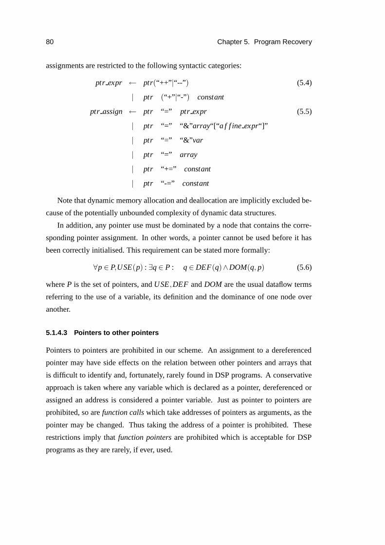
80 Chapter 5. Program Recovery
assignments are restricted to the following syntactic categories:
ptr expr ← ptr(“++”|“--”) (5.4)
| ptr (“+”|“-”) constant
ptr assign ← ptr “=” ptr expr (5.5)
| ptr “=” “&”array“[“a f f ine expr“]”
| ptr “=” “&”var
| ptr “=” array
| ptr “+=” constant
| ptr “-=” constant
Note that dynamic memory allocation and deallocation are implicitly excluded be-
cause of the potentially unbounded complexity of dynamic data structures.
In addition, any pointer use must be dominated by a node that contains the corre-
sponding pointer assignment. In other words, a pointer cannot be used before it has
been correctly initialised. This requirement can be stated more formally:
∀p ∈ P,USE(p) : ∃q ∈ P : q ∈ DEF(q)∧DOM(q, p) (5.6)
where P is the set of pointers, and USE,DEF and DOM are the usual dataflow terms
referring to the use of a variable, its definition and the dominance of one node over
another.
5.1.4.3 Pointers to other pointers
Pointers to pointers are prohibited in our scheme. An assignment to a dereferenced
pointer may have side effects on the relation between other pointers and arrays that
is difficult to identify and, fortunately, rarely found in DSP programs. A conservative
approach is taken where any variable which is declared as a pointer, dereferenced or
assigned an address is considered a pointer variable. Just as pointer to pointers are
prohibited, so are function calls which take addresses of pointers as arguments, as the
pointer may be changed. Thus taking the address of a pointer is prohibited. These
restrictions imply that function pointers are prohibited which is acceptable for DSP
programs as they are rarely, if ever, used.

5.1. Pointer Conversion 81
1. Check Program
(a) Ensure structured loops
(b) Ensure restricted pointer assignment and arithmetic
(c) Check no pointers to pointers
2. Transform
(a) IF legal THEN Gather pointer information using dataflow analysis
(b) IF legal THEN Translate pointers to arrays, remove redundant pointers arithmetic
Figure 5.4: Overall Algorithm
This pointer classification scheme can be realised as a simple, interprocedural non-
iterative algorithm. Any variable identified as a pointer either by its declaration or use,
is labelled as a pointer. The set of pointers is passed into any called function in which
any variable “contaminated” with an already recognised pointer is also included in the
pointer set. If the address of a pointer is taken or a pointed to variable assigned a
pointer value is discovered, the program is rejected. This simple pointer classification
algorithm, described in figure 5.5 will determine potential pointers to pointers occur-
rences. At present, pointer conversion is aborted if any potential pointer to pointer
cases are found.
5.1.4.4 Example
Figure 5.6 shows a program fragment illustrating legal and illegal constructs for pointer
to array conversion. The initialisations of pointers ptr1 and ptr2 are legal; ptr1 is
statically initialised and ptr2 is initialised repeatedly within a loop construct to an
array with an affine subscript.
Pointers ptra, ptrb and ptrc are examples of illegal initialisation; a block of
memory is dynamically allocated and assigned to ptra, whereas the initialisation of
ptrb is illegal because the subscript b[i] is not an affine expression. Finally, the
assignment to ptrc is illegal as there is no dominating definition of ptr.
Pointer arithmetic is restricted in the scheme; the constant increments to pointer

82 Chapter 5. Program Recovery
1. For each procedure P
(a) Forall statements s in the procedure P
i. IF a variable v is declared as a pointer, type * v, used as a pointer * v,assigned
an address of a var, v = & var THEN pointer = pointer ∪v.
(b) Forall statements s in the procedure P
i. IF v,w ∈ pointer and s is of the form * v = w or v = &w THEN my contam =
my contam ∪ { v,w}
ii. return contam = my contam ∩ argument pointers
2. Check (main, /0) where Check (P, inherited pointers) =
(a) Forall statements s in P
i. If s a function call, child contam =child contam ∪ check (s, pointers)
ii. my contam = my contam ∪ child contam
(b) return my contam ∩ arg pointers
3. Propagate (main, /0) where Propagate (P, inherited) =
(a) my contam = my contam ∪ inherited
(b) Forall statements s in P
i. If s a function call, Propagate (s, my contamin∩ actual args)
Figure 5.5: Pointer to pointer analysis

5.1. Pointer Conversion 83
int array1[100], array2[100];
int *ptr1 = &array1[5]; /* OK */
int *ptr2,*ptra,*ptrb,*ptrc,*ptr;
ptra = (int *) malloc(...); /* Not ok */
ptrc = ptr; /* Not ok */
for(i = 0; i < N; i++) {
ptrb = &a[b[i]]; /* Not ok */
ptr2 = &array2[i]; /* OK */
for(j = 0; j < M; j++) {
...
}
ptr1++; /* OK */
ptr1 += 4; /* OK */
}
ptr2 += x; /* Not ok */
ptr2 -= f(y); /* Not ok */
function1(ptr1); /* OK */
function2(&ptr1); /* Not ok */
Figure 5.6: Example of legal and illegal pointer usage

84 Chapter 5. Program Recovery
ptr1 are legal. However the modification of pointer ptr2 is illegal as they include
compile-time unknown values.
Finally, two examples of passing pointers to functions are also shown. function1
receives a pointer to the array, thus only the content of the array can be changed, but
not the pointer ptr1 itself. However, function2 may change the pointer ptr1, which
is not permissible.
5.1.5 Pointer Analysis Algorithm
Once the program has been checked, the second stage of the algorithm gathers infor-
mation on pointer usage before pointer conversion.
5.1.5.1 Dataflow Information
Information on pointer assignments and modifications is stored at each node of the loop
tree. In particular, for each declared pointer, the mapping between this pointer and an
array, including the position of the pointer within the array, is recorded . Additionally,
the label of the node containing the most recent assignment to each pointer is stored.
The data for a pointer p is stored in a tuple of the form ((a,x,n),o1, . . . ,ol) where
a is the array pointed to, x the index of a specific element p points to, n the node the
assignment to p occurred in, ok the movement of the pointer p in a loop k and l the
number of enclosing loops in the function to be analysed.
After initialisation the elements a,x,n and ok carry the default value ⊥ indicating
that no specific information is available. More precisely, ⊥ denotes the state that the
pointer has not been assigned any array element. Conversely, the value > is used to
express the conflict between different assignments. For example, consider the situation
in figure 5.7. Here, in a node of joining control paths the conflict between p pointing
to a along the one incoming path and p pointing to b along another path is resolved
by setting the corresponding element to >. From this it becomes clear that p has been
assigned at least along one control path, but the specific mapping of p is dependent on
the actual program execution path (denoted by > in the corresponding field).
The number of increments of a pointer must be equal across all control paths reach-
ing a particular statement in order that a pointer reference may be replaced by an array

5.1. Pointer Conversion 85
V
p=&a[x] p=&a[y]
p:((a,x,n1),o1) p:((a,y,n2),o2)
n1: n2:
n3:
p:((a,T,T),T)
Figure 5.7: Joining control flow and the meet operator
reference. If the number of increments is different on two joining paths, again this
is denoted by > in the appropriate field. Given this requirement, it is now possible
to define the meet operator, which combines the outcome of following one of two
distinct control-flow paths at the point at which they meet e.g. immediately after an
if-statement. The meet operatorV
is formally defined as follows
^
(((a1,x1,n1),o1,1, . . . ,o1,l),((a2,x2,n2),o2,1, . . . ,o2,l)) (5.7)
=
((a1,x1,n1),o1,1, . . . ,o1,l)
if ((a1,x1,n1),o1,1,...,o1,l)=((a2,x2,n2),o2,1,...,o2,l)
((a1,x1,n1),o1,1, . . . ,>, . . . ,o1,l)
if a1=a2,x1=x2,n1=n2,o1,k 6=o2,k
((a1,>,n1),>, . . . ,>)
if a1=a2,x1 6=x2,n1=n2
((>,>,>),>)
otherwise
This operator is used in section 5.1.5.3 to determine the effects of pointer usage
throughout the program.
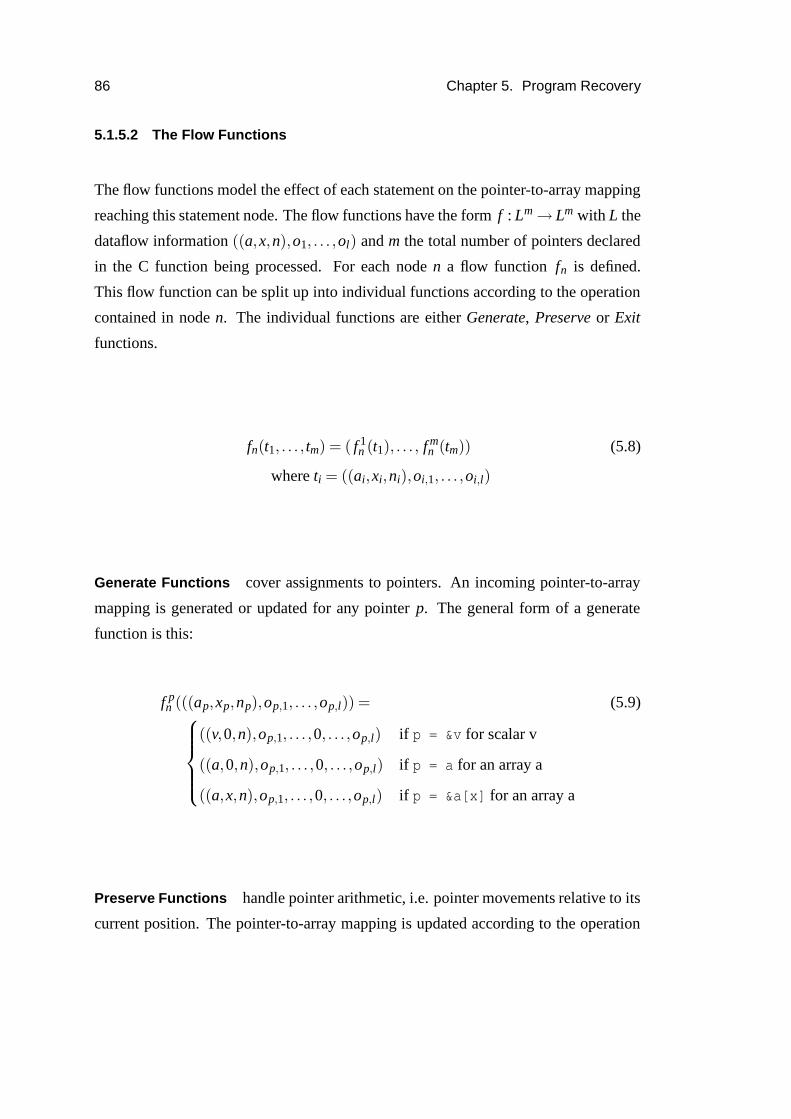
86 Chapter 5. Program Recovery
5.1.5.2 The Flow Functions
The flow functions model the effect of each statement on the pointer-to-array mapping
reaching this statement node. The flow functions have the form f : Lm→ Lm with L the
dataflow information ((a,x,n),o1, . . . ,ol) and m the total number of pointers declared
in the C function being processed. For each node n a flow function fn is defined.
This flow function can be split up into individual functions according to the operation
contained in node n. The individual functions are either Generate, Preserve or Exit
functions.
fn(t1, . . . , tm) = ( f 1n (t1), . . . , f m
n (tm)) (5.8)
where ti = ((ai,xi,ni),oi,1, . . . ,oi,l)
Generate Functions cover assignments to pointers. An incoming pointer-to-array
mapping is generated or updated for any pointer p. The general form of a generate
function is this:
f pn (((ap,xp,np),op,1, . . . ,op,l)) = (5.9)
((v,0,n),op,1, . . . ,0, . . . ,op,l) if p = &v for scalar v
((a,0,n),op,1, . . . ,0, . . . ,op,l) if p = a for an array a
((a,x,n),op,1, . . . ,0, . . . ,op,l) if p = &a[x] for an array a
Preserve Functions handle pointer arithmetic, i.e. pointer movements relative to its
current position. The pointer-to-array mapping is updated according to the operation

5.1. Pointer Conversion 87
of node n.
f pn (((ap,xp,np),op,1, . . . ,op,k, . . . ,op,l)) (5.10)
=
((ap,xp,np),op,1, . . . ,op,k +1, . . . ,op,l)
if p++ and k = inner(n)
((ap,xp,np),op,1, . . . ,op,k−1, . . . ,op,l)
if p-- and k = inner(n)
((ap,xp,np),op,1, . . . ,op,k + c, . . . ,op,l)
if p += c and k = inner(n)
((ap,xp,np),op,1, . . . ,op,k− c, . . . ,op,l)
if p -= c and k = inner(n)
((aq,xq,nq),oq,1, . . . ,oq,k, . . . ,oq,l)
if p = q and q a pointer...
((ap,xp,np),op,1, . . . ,op,k, . . . ,op,l)
otherwise
Exit Functions represent the transition from statement to loop level. Since Exit
nodes occur at the end of a loop body, exit functions have the task of summarising
the effects of the individual statements in the loop body. The result represents the
overall effect of a particular loop level on the pointer mapping.
f pn (((ap,xp,np),op,1, . . . ,op,k, . . . ,op,l)) = (5.11)
((ap,xp,np),op,1, . . . ,op,k, . . . ,op,l)
To compute the total effect of a statement performing pointer arithmetic in a loop
nest, the total number of iterations of each individual loop must be known. Given a
generic loop nest in figure 5.8, the total number of iterations of the innermost loop is
N
∑i0=0
f1(i0)
∑i1=0
f2(i0,i1)
∑i2=0
· · ·fn(i0,...,in−1)
∑in=0
1 (5.12)

88 Chapter 5. Program Recovery
for(i0 = 0; i0 < N; i0 ++)
{
\* pointer incremented by m0,pre * \
for(i1 = 0; i1 < f1(i0); i1 ++)
{
\* pointer incremented by m1,pre * \...
for(in = 0; in < fn(i0, . . . , in−1); in ++)
{
\* pointer incremented by mn *\
}
\* pointer incremented by m1,post * \
}
\* pointer incremented by m0,post * \
}
Figure 5.8: Loop nest with pointer increments

5.1. Pointer Conversion 89
where fk(i0, . . . ik−1) is the number of iterations of the kth nested loop, 1 ≤ k ≤ n. In
the same way, the total number of iterations of an inner loop in level k can be expressed
as
X(k) =N
∑i0=0
f1(i0)
∑i1=0
f2(i0,i1)
∑i2=0
· · ·fk(i0,...,ik−1)
∑ik=0
1 (5.13)
Such terms are frequently encountered in analysing loop nests and can be enumer-
ated using the Omega Calculator (Pugh, 1994) or methods based on Ehrhart polyno-
mials (Clauss, 1996).
Given equations 5.12 and 5.13, the total effect of the pointer increments of a pointer
p in the entire loop nest can be derived as follows:
X(n)×mn+ (5.14)
X(n−1)× (mm−1,pre +mn−1,post)+
. . .
X(0)× (m0,pre +m0,post) =
∑n−1k=0(X(k)×mk,pre +mk,post)+X(n)×mn
where mk,pre,mk,post is the size of the pointer increment in loop k before entering and
after exiting, respectively, the k +1 loop as shown in figure 5.8.
For rectangular iteration spaces and constant numbers of pointer increments on
each loop level, the total number of pointer increments evaluates to affine expressions
dependent on the iteration variables. Otherwise, if all upper loop bounds are affine
expressions in the outer index variables, the resulting expressions are polynomial func-
tions of the index variables.
Once the effects of individual loop levels have been analysed, the pointer conver-
sion algorithm can use this information and compute the total effect of a statement
containing pointer arithmetic in a loop nest. This computation based on the infor-
mation gathered in the analysis stage is part of the conversion algorithm described in
section 5.1.6.

90 Chapter 5. Program Recovery
5.1.5.3 Equation System
The flow functions specify the effects of a statement locally, i.e. on a per node or
statement basis. All flow functions together form an equation system whose solution
is the global dataflow solution. This solution has its representation in the IN[n] and
OUT [n] sets associated with each node.
Solving the dataflow equation starts with all pointers initialised to a default value,
i.e.
∀p : ((ap,xp,np),op,1, . . . ,op,l) = ((⊥,⊥,⊥),⊥) (5.15)
resulting in
IN[n] = (((⊥,⊥,⊥),⊥), . . . ,((⊥,⊥,⊥),⊥)) (5.16)
The equation system is solved by visiting all nodes in reverse postorder beginning
at the start node no and computing the IN[n] and OUT [n] sets as follows:
OUT [n] = fn(IN[n]) (5.17)
IN[n] =^
m∈pred(n)
OUT [m] (5.18)
Only a single iteration is required to propagate the pointer mapping values. Thus,
its runtime complexity is O(N) with N the number of nodes in the CFG. Unlike iterative
dataflow analysis this algorithm does not compute any fix point. The transition from
statement to loop level is done at the end of the loop body when the flow function of
the loop node is computed.
5.1.6 Pointer Conversion Algorithm
In a second pass over the CFG, step 2b in the algorithm, pointer accesses and arith-
metic are replaced and removed, respectively. Replacement is based on the dataflow
information gathered during the analysis stage. From this information, the index ex-
pressions of the array accesses are constructed.
A pointer reference can only be replaced if its array a and offset o components of
the tuple ((a,x, l),o1, . . . ,ol) are unambiguous. This is the case when a,o 6∈ {⊥,>}.

5.1. Pointer Conversion 91
The information required for the conversion of a pointer access into an array access
is contained in the computed dataflow values IN. The necessary components for the
construction of the array access are:
1. The array name A,
2. the initial offset at the location of the first pointer assignment offsetinit ,
3. and a linear expression in outer iterators f (i1, . . . , ilevel).
Figure 5.9 shows the pointer conversion algorithm. It operates on the loop nest
from the innermost loop to the outermost loop. On each level each pointer-based access
is analysed, and an explicit array access replacing the original access is constructed.
Information is gathered from the IN sets of the current node and the exit nodes of the
enclosing loops. Based on this information, the new access is computed.
If there are uses of the pointer following the transformed loop which cannot be
eliminated by the pointer conversion algorithm, an additional statement with an update
of the pointer taking into account the total effect of the loop on the pointer must be
inserted immediately after the loop.
The example in the following section illustrates the application of the pointer con-
version algorithm on the matrix1 program.
5.1.7 Example
In figure 5.10, each node of the matrix1 program together with its associated dataflow
information for the pointer p c is shown. The rightmost column (p c→ c) of figure
5.10 contains the expressions, which together form the explicit array access, and are
constructed during pointer conversion.
From the IN set of node 8, the mapping of pointer p c onto the array C can be read
off. Additionally, the initial offset offsetinit = 0 and the entry offset offsetentry = 0 are
stored at this node. The contributions to linear function f come from the exit nodes of
the surrounding loops. Putting together the subexpressions as described in the previous
section results in the explicit memory access C[k∗X + i] for node 8. In a similar way the
assignment *p c = 0 in node 6 can be replaced. After the replacement of all accesses

92 Chapter 5. Program Recovery
• From inner loop to outer loop:
1. For all pointer-based accesses in loop-level level
(a) Select next pointer-based access based on pointer p in node n
(b) Construction of explicit array reference A[I]
i. Inspect IN pn = ((a,x, l),o1 , . . . ,ol)),a,x, l,ok 6∈ {⊥,>}.
ii. Determine array A = a.
iii. Determine index I = offset init +offsetentry + f (i1, . . . , ilevel ).
A. Determine offset init = x.
B. Determine offsetentry = ∑leveli=1 oi.
C. Determine linear function f (i1, . . . , ilevel ).
f (i1, . . . , ilevel ) =
0, if ok =⊥,∀k
0, if ok = 0,∀k
∑levelk=1 X(k)×o′k where o′k from IN p
exitk
if inner(n) =⊥
∑levelk=1 X(k)× ck
if n is re-assigned in loop level l
and ck =
0, if k ≤ level
o′k from IN pexitk
,otherwise
(c) Replace pointer-based access with A[I]
2. Delete all pointer expressions modifying p from loop
Figure 5.9: Pointer Conversion Algorithm
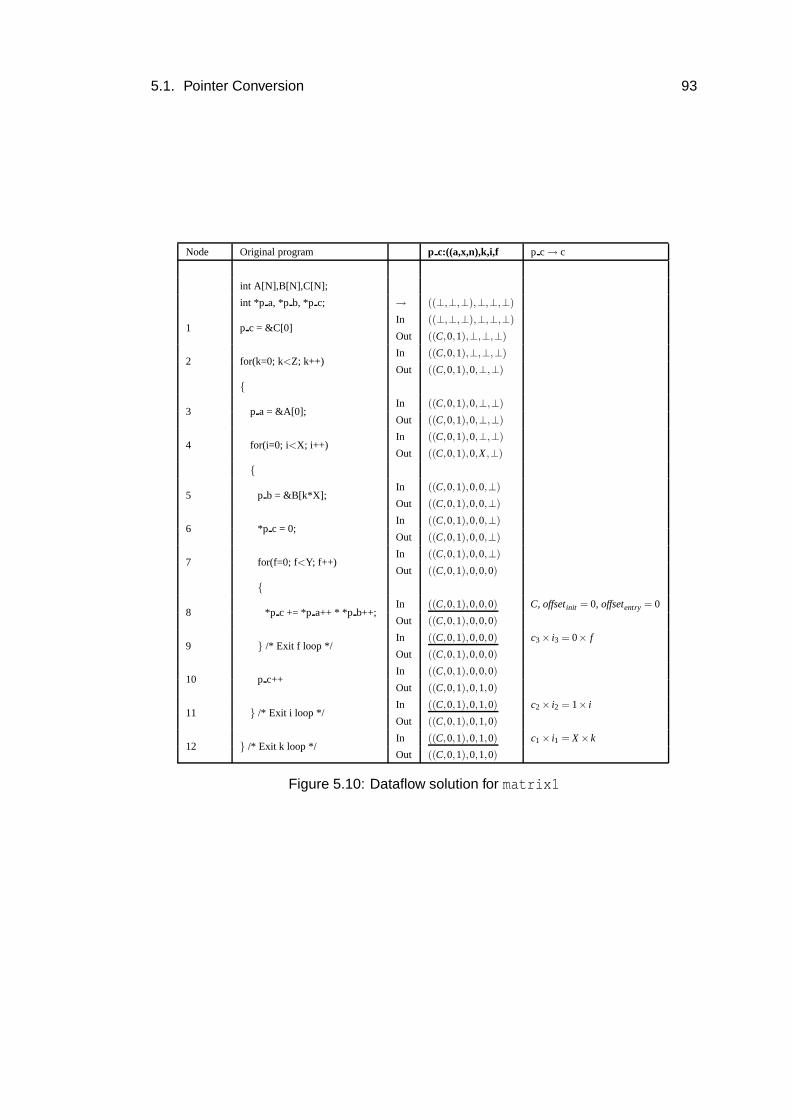
5.1. Pointer Conversion 93
Node Original program p c:((a,x,n),k,i,f p c→ c
int A[N],B[N],C[N];
int *p a, *p b, *p c; → ((⊥,⊥,⊥),⊥,⊥,⊥)
1 p c = &C[0]In ((⊥,⊥,⊥),⊥,⊥,⊥)
Out ((C,0,1),⊥,⊥,⊥)
2 for(k=0; k<Z; k++)In ((C,0,1),⊥,⊥,⊥)
Out ((C,0,1),0,⊥,⊥)
{
3 p a = &A[0];In ((C,0,1),0,⊥,⊥)
Out ((C,0,1),0,⊥,⊥)
4 for(i=0; i<X; i++)In ((C,0,1),0,⊥,⊥)
Out ((C,0,1),0,X ,⊥)
{
5 p b = &B[k*X];In ((C,0,1),0,0,⊥)
Out ((C,0,1),0,0,⊥)
6 *p c = 0;In ((C,0,1),0,0,⊥)
Out ((C,0,1),0,0,⊥)
7 for(f=0; f<Y; f++)In ((C,0,1),0,0,⊥)
Out ((C,0,1),0,0,0)
{
8 *p c += *p a++ * *p b++;In ((C,0,1),0,0,0) C, offsetinit = 0, offsetentry = 0
Out ((C,0,1),0,0,0)
9 } /* Exit f loop */In ((C,0,1),0,0,0) c3× i3 = 0× f
Out ((C,0,1),0,0,0)
10 p c++In ((C,0,1),0,0,0)
Out ((C,0,1),0,1,0)
11 } /* Exit i loop */In ((C,0,1),0,1,0) c2× i2 = 1× i
Out ((C,0,1),0,1,0)
12 } /* Exit k loop */In ((C,0,1),0,1,0) c1× i1 = X× k
Out ((C,0,1),0,1,0)
Figure 5.10: Dataflow solution for matrix1

94 Chapter 5. Program Recovery
via the pointer p c, the statements containing pointer arithmetic on p c can be deleted.
Finally, after ensuring that no further use of p c remains, the declaration of the pointer
can be discarded. p a and p b are treated in a similar manner. The final program is
shown in figure 5.2.
This example will be used as a running example throughout this thesis. In section
5.3, both the original and the transformed version of the the program are juxtaposed
and further discussed.
5.2 Modulo Removal
Modulo addressing is a frequently occurring idiom in DSP programs. In this section,
a new technique to remove modulo addressing by transforming the program into an
equivalent linear form, if one exists, is developed. This transformation uses rank-
modifying transformation framework (O’Boyle and Knijnenburg, 2002), which ma-
nipulates extended linear expressions including mods and divs. In O’Boyle and Kni-
jnenburg (2002) this was mainly used to reason about reshaped arrays, here it is used
to formalise a program recovery technique.
Modulo recovery is also considered in Balasa et al. (1994) where a large, highly
specialised framework based on Diophantine equations is presented to solve modulo
accesses. It, however, introduces costly floor, div and ceil functions and its effect
on other parts of the program is not considered.
In section 5.2.1, a simple example is used to motivate the following work. Before
the modulo removal algorithm is presented in section 5.2.4, a short introduction to the
used notation is given in section 5.2.2. Assumptions and known restrictions of the
modulo removal are described in 5.2.3. A larger example is given towards the end of
this chapter in section 5.2.5.
5.2.1 Motivation
The code in figure 5.11, box (1), is typical of C programs written for DSP processors
and contains fragments from the UTDSP benchmark suite. Circular buffer access is a
frequently occurring idiom in DSP programs and is typically represented as a modulo

5.2. Modulo Removal 95
expression in one or more of the array subscripts as can be seen in the second loop
nest. Such non-linear expressions will again defeat most data dependence techniques
and prevent further optimisation and parallelisation.
In the presented program recovery scheme, the modulo accesses are removed by
applying a suitable strip-mining transformation to give the new code in box (2), figure
5.11. Repeated strip-mining gives the code in box (3).
5.2.1.1 Benefit of Modulo Removal
The modulo-free form is now amendable to further analysis and transformation. Al-
though the new code contains linear array subscripts, these are easily optimised by
code hoisting and strength reduction in standard native compilers.
Another possibility of taking advantage of the modulo-free form of the program
comes from the fact that the order of memory accesses has not been changed by the
employed strip-mining transformation. This implies that any data flow information
valid for a modulo-free form is also valid for the original version of a given program.
As a consequence, results from an array data flow analysis (e.g. Duesterwald et al.,
1993) can be transferred from the modulo-free program back to the original code.
Knowledge of the dependence information enables other transformations, including
parallelisation, while retaining the modulo-based accesses for further processing (e.g.
exploitation of modulo-addressing modes of the AGUs, see 2.2.2.2).
5.2.2 Notation
Before the modulo removal algorithm is described, the notation used in this section is
introduced. The loop iterators can be represented by a column vector III = [i1, i2, . . . , iM]T
where M is the number of enclosing loops. Note the loops do not need to be perfectly
nested and occur arbitrarily in the program. The loop ranges are described by a system
of inequalities defining the polyhedron or iteration space BIII ≤ bbb. The data storage of
an array can also be viewed as a polyhedron. Array indices JJJ = [ j1, j2, . . . , jN]T are
used to describe the array index space. This space is given by the polyhedron AJJJ ≤ aaa.
It is assumed that the subscripts in a reference to an array can be written as UIII + uuu,
where U is an integer matrix and uuu is a vector. Thus in figure 5.11, box(3) the array

96 Chapter 5. Program Recovery
int e[32][32], f[32], g[32][8], h[32][4];
for (i = 0 ; i < 32 ; i++) {
for (j = 0 ; j < 32 ; j++) {
e[i][j] = f[i] * g[i][j%8] * h[i][j%4];
}
}
(1) Original Code
int e[32][32], f[32], g[32][8], h[32][4];
for (i = 0 ; i < 32 ; i++) {
for (j1 = 0 ; j1 < 4 ; j1++) {
for (j2 = 0 ; j2 < 8 ; j2++) {
e[i][8*j1+j2] = f[i] * g[i][j2] * h[i][j2%4];
}
}
}
(2) Code after strip-mining
int e[32][32], f[32], g[32][8], h[32][4];
for (i = 0 ; i < 32 ; i++) {
for (j1 = 0 ; j1 < 4 ; j1++) {
for (j2 = 0 ; j2 < 2 ; j2++) {
for (j3 = 0 ; j3 < 4 ; j3++) {
e[i][8*j1+4*j2+j3] = f[i] * g[i][4*j2+j3] * h[i][j3];
}
}
}
}
(3) Code after repeated strip-mining
Figure 5.11: Example showing Modulo Removal

5.2. Modulo Removal 97
declaration f[32] is represented by[
−1
1
]
[ j1]≤
[
0
31
]
(5.19)
i.e. the index j1 ranges over 0≤ i1 ≤ 31. The loop bounds are represented in a similar
manner and the subscript of f, f[i], is simply
[
1 0]
[
i1
i2
]
+
[
0
0
]
(5.20)
When discussing larger program structures, the notion of computation sets is use-
ful, where Q = (BIII ≤ bbb,(si|Qi)) is a computation set consisting of the loop bounds,
BIII ≤ bbb and either enclosed statements (s1, . . . ,sn) or further loop nests (Q1, . . . ,Qn).
5.2.3 Assumptions and Restrictions
The algorithm is restricted to simple modulo expressions of the syntactic form
(aρ× iρ)%cρ (5.21)
where iρ is an iterator, and aρ,cρ are constants and ρ∈ 1, . . . ,m is the index of the refer-
ence containing the modulo expression. More complex references are highly unlikely
but may be addressed by extending the approach below to include skewing.
Furthermore, it is assumed that all constants c j are integer multiples of each other,
i.e. ∃k : lcm(c1, . . . ,cm) = ck. Although this restriction might appear serious, prac-
tically it does not restrict the applicability and effectiveness of the modulo removal
algorithm. In fact, many DSP programs only maintain one circular buffer per loop and
even in those with more than one, the buffer sizes are often related as required.
5.2.4 Modulo Removal Algorithm
In this section, the modulo removal algorithm is described and discussed. The algo-
rithm itself is presented in figure 5.12. Essentially, the algorithm performs a number
of strip-mining transformations to eliminate modulo operations in index functions of
array accesses before it outputs the modulo-free program.

98 Chapter 5. Program Recovery
1. Construction of the Computation Set Q = (BIII ≤ bbb,(si|Qi))
(a) Construction of the Equation System of the loop under consideration
(b) Matrix Representation of the equation system BIII ≤ bbb
2. Construction of the Generalised Strip-Mining Matrix S
(a) Computation of the Least Common Multiple l = lcm(c1, . . . ,cm)
(b) Construction of the Special Transformation Matrix
Sl =
[
(.)/l
(.)%l
]
and the Special Pseudo-Inverse
S†l =
[
l 1]
(c) Construction of the Generalised Strip-Mining Matrix S and its Pseudo-Inverse S †
S =
Id k−1 0 0
0 Sl 0
0 0 IdN−k
and S† =
Id k−1 0 0
0 S†l 0
0 0 IdN−k
3. Computation of new Iteration Space and Loop Bounds
(a) Computation of new loop Bounds bbb′′′ =
[
Id 0
0 S
]
bbb
(b) Computation of new loop Iterators III′′′ = SIII
(c) Computation of new Coefficients B′ = XBS † , where X =
[
S 0
0 S
]
(d) Construction of new Equation System B ′III′′′ ≤ bbb′′′
4. Update of Array References
(a) Update all Array References U ′ = US † in si
5. Go to step 1, until all modulo operations in array accesses have been removed.
Then proceed with step 6.
6. Code Generation
Figure 5.12: Modulo Removal Algorithm

5.2. Modulo Removal 99
In step 1 of the algorithm, the computation set Q of the loop under consideration
is constructed. For this, an equation system describing the iteration space and loop
bounds is constructed (step 1a) and expressed in matrix representation (step 1b). Step
2 serves as a precomputation stage, in which the Generalised Strip-Mining Matrix
S and its Pseudo-Inverse S† are computed. These matrices are constructed of the
Special Strip-Mining Matrix Sl and its Pseudo-Inverse (step 2b), which in turn rely
on the least common multiple l of the constants c j from array index functions (a j×
i j)%c j (step 2a). Then a loop strip-mining transformation S is applied to the loop nest
(step 3). The particular formulation used is based on rank-modifying transformations
(O’Boyle and Knijnenburg, 2002), which unify loop and data transformations in an
algebraic transformation framework. New loop bounds B ′ (step 3a), iterators (step
3b) and coefficients (step 3c) are computed and together they describe the polyhedron
B′III′′′ ≤ bbb′′′. In step 4 the array accesses are updated to represent the new loop indices.
Remaining modulo operations are eliminated by iterating over steps 1-4 until no more
modulos can be found in any array index function. Finally, a code generation stage
outputs the transformed program for further processing.
As most DSP programs contain only a very small number of different modulo con-
stants c j, the algorithm usually terminates after only one or two iterations. In general,
the number of iterations is bounded by the number m of modulo accesses in the loop
body. The cost of a single iteration is dominated by the computation of the new coef-
ficients (step 3c), which is dependent on the size of the matrix S . As the size of the
matrix S is bounded by the dimension N of the index space (step 2c), the computation
in step 3c has asymptotic cost O(N3). Thus, the overall runtime of the modulo removal
algorithm is O(m×N3). Usually, both m and N are very small and fixed, such that the
algorithm has nearly constant runtime for almost all practical problems.
The memory requirements of the modulo removal algorithm mainly originate from
the matrices to be stored. As before, the cost are dominated by the matrix S . Conse-
quently, the overall memory requirement is bounded by O(N2).

100 Chapter 5. Program Recovery
5.2.5 Example
In this section, the previously presented algorithm is applied to the example in figure
5.11, box (1).
1. Construction of the Computation Set Q.
(a) Equation System.
(−1)i+0 j ≤ 0
0i+(−1) j ≤ 0
1i+0 j ≤ 31
0i+1 j ≤ 31
(b) Matrix Representation BIII ≤ bbb.
−1 0
0 −1
1 0
0 1
[
i
j
]
≤
0
0
31
31
2. Construction of the Generalised Strip-Mining Matrix S .
(a) Computation of the Least Common Multiple l.
Let l be the least common multiple of c j. In figure 5.11, box(1), it is c1 = 8,
c2 = 4 from the access to g and h and hence l = 8.
(b) Construction of Sl and S†l .
S8 =
[
(.)/8
(.)%8
]
S†8 =
[
8 1]

5.2. Modulo Removal 101
(c) Construction of S and S†.
S =
1 0
0 (.)/8
0 (.)%8
S† =
[
1 0 0
0 8 1
]
3. Computation of new Iteration Space and Loop Bounds
(a) Computation of bbb′′′ =
[
Id 0
0 S
]
bbb.
bbb′′′ =
1 0 0 0
0 1 0 0
0 0 0 0
0 0 1 0
0 0 0 (.)/8
0 0 0 (.)%8
0
0
31
31
=
0
0
0
31
3
7
(b) Computation of III′′′ = SIII.
III′′′ =
1 0
0 (.)/8
0 (.)%8
[
i
j
]
=
i
j/8
j%8
=
i
j1
j2

102 Chapter 5. Program Recovery
(c) Computation of B′ = XBS
†, where X =
[
S 0
0 S
]
.
B′ =
1 0 0 0
0 (.)/8 0 0
0 (.)%8 0 0
0 0 1 0
0 0 0 (.)/8
0 0 0 (.)%8
−1 0
0 −1
1 0
0 1
[
1 0 0
0 8 1
]
=
−1 0
0× (.)/8 −1× (.)/8
0× (.)%8 −1× (.)%8
1 0
0× (.)/8 1× (.)/8
0× (.)%8 1× (.)%8
[
1 0 0
0 8 1
]
=
−1 0 0
0 −1 0
0 0 −1
1 0 0
0 1 0
0 0 1
(d) Construction of Equation System B ′III′′′ ≤ bbb′′′.
−1 0 0
0 −1 0
0 0 −1
1 0 0
0 1 0
0 0 1
i
j1
j2
≤
0
0
0
31
3
7
4. Update of Array References
(a) Update all Array References U ′ = US† in si.

5.2. Modulo Removal 103
i. Array reference: e[i][j]
From this reference
UIII +uuu =
[
1 0
0 1
][
i
j
]
+
[
0
0
]
=
[
1i+0
1 j +0
]
and
U′ =
[
1 0
0 1
][
1 0 0
0 8 1
]
=
[
1 0 0
0 8 1
]
are constructed. So the new reference becomes U ′III′′′+uuu =
[
1 0 0
0 8 1
]
i
j1
j2
+
[
0
0
]
=
[
i
8 j1 +1 j2
]
i.e. e[i][8*j1+j2].
ii. Array reference: f[i]
The one-dimensional reference f[i] is considered as a shortform of
the multi-dimensional reference f[i][0]. As before
UIII +uuu =
[
1 0
0 0
][
i
j
]
+
[
0
0
]
=
[
1i+0
0 j +0
]
and
U′ =
[
1 0
0 0
][
1 0 0
0 8 1
]
=
[
1 0 0
0 0 0
]
are constructed. Thus, the new reference is U ′III′′′+uuu =
[
1 0 0
0 0 0
]
i
j1
j2
+
[
0
0
]
=
[
i
0
]
i.e. f[i][0] or f[i], respectively.
iii. Array reference: g[i][j%8]
Again,
UIII +uuu =
[
1 0
0 (.)%8
][
i
j
]
+
[
0
0
]
=
[
1i+0
0i+ j%8
]

104 Chapter 5. Program Recovery
and
U′ =
[
1 0
0 (.)%8
][
1 0 0
0 8 1
]
=
[
1 0 0
0 0 1
]
are constructed. The new reference becomes U ′III′′′+uuu =
[
1 0 0
0 0 1
]
i
j1
j2
+
[
0
0
]
=
[
i
j2
]
i.e. g[i][j2].
iv. Array reference: h[i][j%4]
Analogously,
UIII +uuu =
[
1 0
0 (.)%4
][
i
j
]
+
[
0
0
]
=
[
1i+0
0i+ j%4
]
and
U′ =
[
1 0
0 (.)%4
][
1 0 0
0 8 1
]
=
[
1 0 0
0 8(.)%4 1(.)%4
]
Thus, U ′III′′′+uuu =
[
1 0 0
0 8(.)%4 1(.)%4
]
i
j1
j2
+
[
0
0
]
=
[
i
8( j1)%4+1( j2%4)
]
Since 8( j1)%4 = 0,∀ j1 the new reference turns out to be h[i][j2%4].
5. At this stage all but one modulo operation in array references have been elim-
inated. The program has been transformed into the form shown in figure 5.11,
box (2). A further iteration of the strip-mining transformation (not presented
here) eliminates the last modulo expression.
6. Code Generation
The result of this stage is shown in figure 5.11, box (3).

5.3. Running Example 105
5.3 Running Example
In this section a real-world example program that will be used throughout this thesis
is introduced. It will be used to demonstrate different program transformation tech-
niques. matrix1 is a matrix multiplication kernel from the DSPstone benchmark suite
(Zivojnovic et al., 1994). Starting with the original pointer-based version, all transfor-
mations stages necessary to obtain a parallel high-performance implementation will be
shown in the following chapters of this thesis.
static TYPE A[X*Y] ;
static TYPE B[Y*Z] ;
static TYPE C[X*Z] ;
STORAGE CLASS TYPE *p a = &A[0] ;
STORAGE CLASS TYPE *p b = &B[0] ;
STORAGE CLASS TYPE *p c = &C[0] ;
STORAGE CLASS TYPE f,i,k ;
for (k = 0 ; k < Z ; k++)
{
p a = &A[0] ; /* point to the beginning of array A */
for (i = 0 ; i < X; i++)
{
p b = &B[k*Y] ; /* take next column */
*p c = 0 ;
for (f = 0 ; f < Y; f++) /* do multiply */
*p c += *p a++ * *p b++ ;
p c++ ;
}
}
Figure 5.13: Pointer-based matrix1 program from DSPstone

106 Chapter 5. Program Recovery
static TYPE A[X*Y] ;
static TYPE B[Y*Z] ;
static TYPE C[X*Z] ;
STORAGE CLASS TYPE f,i,k ;
for (k = 0 ; k < Z ; k++)
{
for (i = 0 ; i < X; i++)
{
C[k*X+i] = 0 ;
for (f = 0 ; f < Y; f++) /* do multiply */
C[k*X+i] += A[i*Y+f] * B[k*Y+f] ;
}
}
Figure 5.14: matrix1 after Pointer Conversion
5.3.1 Pointer Conversion
The initial matrix multiplication kernel matrix1 from the DSPstone benchmark suite is
presented in figure 5.13. Two matrices stored in the linear arrays A and B are multiplied,
and the resulting matrix is stored in the array C.
The code has been manually tuned to assist the compiler in effective address code
generation and vectorisation of the innermost loop. The code makes extensive use of
pointer arithmetic for array traversals such that even a simple compiler can immedi-
ately map pointer increments onto post-increment addressing operations provided by
DSP architectures. Furthermore, the matrix A is stored row-wise, whereas matrices
B and C are stored column-wise in linear arrays. As a result of this data layout, the
innermost loop is easily vectorisable for a DSP with SIMD capabilities. However,
these program transformations are only able to support relative poor compilers at the
cost of obfuscating the programmer’s original intention. More sophisticated compil-
ers with advanced built-in transformations are most likely to fail to achieve optimal

5.3. Running Example 107
performance, since their analyses are not designed to cope with code written in this
style.
Application of pointer conversion as described earlier in this chapter produces the
code in figure 5.14. The pointer-based accesses to the arrays A, B and C have been
replaced by equivalent explicit array accesses. Pointer declarations and initialisations
have been dropped. The array-based version of the code is amendable to array dataflow
analysis enabled transformations, whereas many compilers fail to optimise the pointer-
based code.
Details of the analysis and conversion of this example program can be found in
section 5.1.
5.3.2 Modulo Removal
Modulo removal is not only useful as a preprocessing stage, but can also support
eliminating modulo index expression introduced by other transformations. Again, the
matrix1 program is taken to illustrate this purpose.
During later stages of parallelisation the code presented in figure 5.15 is generated
(see also section 7.5.5). The arrays A, B and C have been transformed from originally
one dimension in figure 5.13 to three dimensions, and the references to the three arrays
have been adjusted. Due to strip-mining of the k-loop, two new loops have been cre-
ated: The outer k1-loop, which has been distributed across several processors and has
no explicit representation in the code in figure 5.15, and the inner k2-loop with Z/4
iterations. A constant MYID has been introduced to represent individual iterations of
the implicit k1 loop. References to arrays B and C are affine, but the reference to the
array A contains non-linear mod and div expressions.
Strip-mining the i loop by X/4 and updating the array references accordingly, re-
sults in the program shown in figure 5.16. Potentially expensive and analysis defeating
mod and div expressions have been traded in against another level of loop nesting.
The index expression of the reference to C has become slightly more complex, but is
still within the “compiler-friendly” class of affine expressions in outer loop induction
variables.
A step-by-step description of the calculations carried out to transform the program
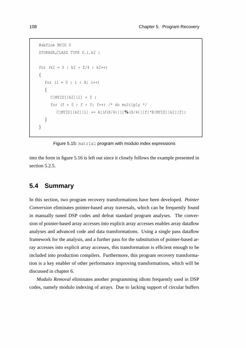
108 Chapter 5. Program Recovery
#define MYID 0
STORAGE CLASS TYPE f,i,k2 ;
for (k2 = 0 ; k2 < Z/4 ; k2++)
{
for (i = 0 ; i < X; i++)
{
C[MYID][k2][i] = 0 ;
for (f = 0 ; f < Y; f++) /* do multiply */
C[MYID][k2][i] += A[i/(X/4)][i%(X/4)][f]*B[MYID][k2][f];
}
}
Figure 5.15: matrix1 program with modulo index expressions
into the form in figure 5.16 is left out since it closely follows the example presented in
section 5.2.5.
5.4 Summary
In this section, two program recovery transformations have been developed. Pointer
Conversion eliminates pointer-based array traversals, which can be frequently found
in manually tuned DSP codes and defeat standard program analyses. The conver-
sion of pointer-based array accesses into explicit array accesses enables array dataflow
analyses and advanced code and data transformations. Using a single pass dataflow
framework for the analysis, and a further pass for the substitution of pointer-based ar-
ray accesses into explicit array accesses, this transformation is efficient enough to be
included into production compilers. Furthermore, this program recovery transforma-
tion is a key enabler of other performance improving transformations, which will be
discussed in chapter 6.
Modulo Removal eliminates another programming idiom frequently used in DSP
codes, namely modulo indexing of arrays. Due to lacking support of circular buffers

5.4. Summary 109
#define MYID 0
STORAGE CLASS TYPE f,i1,i2,k2 ;
for (k2 = 0 ; k2 < Z/4 ; k2++)
{
for (i1 = 0 ; i1 < 4; i1++)
{
for (i2 = 0; i2 < X/4; i2++)
{
C[MYID][k2][(X/4)*i1+i2] = 0 ;
for (f = 0 ; f < Y; f++) /* do multiply */
C[MYID][k2][(X/4)*i1+i2] += A[i1][i2][f] * B[MYID][k2][f];
}
}
}
Figure 5.16: matrix1 program after modulo removal
in the C programming language, programmers frequently resort to difficult to analyse
modulo-based array indexing. While this approach is portable, the resulting code is
often very inefficient. The modulo removal transformation introduced in this chapter
eliminates modulo indexing by strip-mining the surrounding loop appropriately. The
transformed index expressions are affine and can be analysed using standard array
dataflow analyses. This opens up the opportunity for further performance enhancing
transformations.
In chapter 6, the application and effectiveness of both program recovery transfor-
mations developed in this chapter are discussed based on the empirical evaluation of a
DSP-specific benchmark suite.


Chapter 6
High-Level Transformations for
Single-DSP Performance Optimisation
Efficient implementation of DSP applications is critical for many embedded systems.
Optimising C compilers largely focus on code generation and scheduling, which, with
their growing maturity, are providing diminishing returns. In this chapter another
approach based on high-level source-to-source transformations is empirically evalu-
ated. While program performance already benefits from the application of individual
transformations, the full potential is only realised when several transformations are
combined. However, the identification of a successful transformation sequence is a
non-trivial task and static approaches often fail due to the complex interaction be-
tween high-level transformations, the backend compiler and the target architecture.
Furthermore, static analysis is usually prohibited by the fact that compiler manufactur-
ers rarely document the low-level transformations applied by their compilers. Iterative
exploration of the transformation space, on the other hand, does not assume any knowl-
edge of the backend compiler and is yet able to find effective transformation sequences.
This is achieved by alternating transformation and execution stages and selecting the
best option afterwards.
High-level techniques are applied to the DSPstone benchmarks on four platforms:
TriMedia TM-1000, Texas Instruments TMS320C6201, Analog Devices SHARC ADSP-
21160 and TigerSHARC TS101. On average, the best transformations give a factor of
111

112 Chapter 6. High-Level Transformations for Single-DSP Performance Optimisation
2.21 improvement across the platforms. In certain cases a speedup of 5.48 is found
for the SHARC, 2.95 on the TigerSHARC, 7.38 for the TM-1 and 2.3 for the C6201.
These results certainly justify further investigation into the use of high-level techniques
for embedded systems compilers.
6.1 Introduction
Digital signal processing and media processing are performance critical applications
for embedded processors. This demand for performance has led to the development
of specialised architectures (see section 2.2), with application programs hand-coded in
assembly. More recently as the cost of developing an embedded system becomes dom-
inated by algorithm and software development, there has been a move towards the use
of high-level programming languages, in particular C. As in other areas of computing,
programming in C is much less time consuming than hand-coded assembler, but this
comes at the price of a less efficient implementation when compared to hand-coded
approaches (Frederiksen et al., 2000).
To trade off the often conflicting goals of reducing application development time
and increasing code performance there has been much interest in optimising compiler
technology, where the compiler is responsible for automatically “tuning” the program
(de Araujo, 1997; Leupers, 1998; Timmer et al., 1995; Sair et al., 1998; Bhattacharyya
et al., 2000). This work has primarily focused on efficient code generation or schedul-
ing of the low-level instructions.
However, code generation and to a lesser extent scheduling are platform specific.
More significant is the fact that they are relatively mature techniques and there is a
diminishing rate of return for increasingly sophisticated approaches. In Timmer et al.
(1995), for instance, a scheduler is developed for a particular in-house core that is
optimal in the majority of cases. Thus, if performance is to be increased further, it is
worth considering alternative approaches.
One such approach is to examine high-level transformations. These are inher-
ently portable and have been shown to give significant performance improvement for
general-purpose processors (Kisuki et al., 2000), yet there is little work on their im-
6.1. Introduction 113
pact on embedded applications perhaps due to the historical bottom-up approach to
embedded systems.
One major difficulty in the use of high-level transformations is that the preferred
application language is C, which is not very well suited to optimisations. Extensive
usage of pointer arithmetic (Liem et al., 1996; Zivojnovic et al., 1994; Numerix, 2000)
prevents the application of well developed array-based dataflow analyses and transfor-
mations. However, in section 5.1 of this thesis a technique to transform pointer-based
programs into an equivalent array-based form has been developed, which opens the
opportunity for the application of more extensive high-level transformations.
There has been limited work in the evaluation of high-level transformations on
embedded systems performance. In Bodin et al. (1998) the tradeoff between code
size and execution time of loop unrolling has been investigated and in Kandemir et al.
(2000) the impact of tiling on power consumption has been evaluated. Although power
consumption and also code size are very important issues for embedded systems they
are not the primary focus of this work. Rather the focus is on techniques to improve
execution time assuming a fixed amount of embedded memory. The impact of sev-
eral high-level transformations on the DSPstone (Zivojnovic et al., 1994) benchmark
suite is empirically evaluated on four different embedded processors. It is shown that
by selecting the appropriate sequence of transformations in an iterative transformation
framework, average execution time can be improved by a factor of 2.43, justifying fur-
ther investigation of high-level transformations within embedded systems compilers.
This chapter is organised as follows. Section 6.2 provides a motivating example
illustrating the application and effect of high-level transformations. Section 6.3 de-
scribes the transformations investigated and is followed in section 6.4 by an example.
The evaluation of individual transformations is covered in section 6.5. A description
of an iterative search strategy which finds “good” transformation sequences is given in
section 6.6. In section 6.7 the results for combined transformations are presented and
analysed. A discussion of related work can be found in section 6.8, and section 6.9
concludes.

114 Chapter 6. High-Level Transformations for Single-DSP Performance Optimisation
6.2 Motivation
Pointer conversion, a program recovery transformation presented and discussed in sec-
tion 5.1, is a key enabler of many other program transformations. For instance, con-
sider figure 6.11, a kernel loop of the DSPstone benchmark matrix2.c. In a misguided
attempt to “optimise” the code generation for this program, the programmer has in-
troduced pointer accesses to array elements and pointer arithmetic to express linear
array traversals. However, an advanced compiler with built-in array dataflow analyses
might often fail to achieve optimal performance due to conservative assumptions about
pointer aliasing.
int *p a = &A[0] ;
int *p b = &B[0] ;
int *p c = &C[0] ;
for (k = 0 ; k < Z ; k++) {
p a = &A[0] ;
for (i = 0 ; i < X; i++) {
p b = &B[k*Y] ;
*p c = *p a++ * *p b++ ;
for (f = 0 ; f < Y-2; f++)
*p c += *p a++ * *p b++ ;
*p c++ += *p a++ * *p b++ ;
}
}
Figure 6.1: Original pointer-based array traversal
Figure 6.2 shows the loop after pointer conversion, i.e. pointer-based accesses
and pointer arithmetic have been substituted by explicit array accesses. Once in an
array-based form, further program transformations may also be applied. Figure 6.3
shows the example loop after application of pointer conversion and delinearisation.
1For convenience reasons figures 5.1 and 5.2 from section 5.1 have been duplicated here.

6.3. High-Level Transformations 115
for (k = 0 ; k < Z ; k++) {
for (i = 0 ; i < X; i++) {
C[X*k+i] = A[Y*i] * B[Y*k];
for (f = 0 ; f < Y-2; f++)
C[X*k+i] += A[Y*i+f+1] * B[Y*k+f+1];
C[X*k+i] += A[Y*i+Y-1] * B[Y*k+Y-1];
}
}
Figure 6.2: After conversion to explicit array accesses
Delinearisation is the transformation of one-dimensional arrays into multi-dimensional
arrays (O’Boyle and Knijnenburg, 2002). In this example, the arrays A, B and C are now
two-dimensional arrays. This data representation enables more aggressive compiler
transformations such as data layout optimisations (O’Boyle and Knijnenburg, 2002).
for (k = 0 ; k < Z ; k++) {
for (i = 0 ; i < X; i++) {
C[k][i] = A[i][0] * B[k][0];
for (f = 0 ; f < Y-2; f++)
C[k][i] += A[i][f+1] * B[k][f+1];
C[k][i] += A[i][Y-1] * B[k][Y-1];
}
}
Figure 6.3: Example loop after delinearisation
6.3 High-Level Transformations
Converting pointer-based programs enables a number of powerful high-level transfor-
mations. The transformations investigated are selected based on the characteristics of

116 Chapter 6. High-Level Transformations for Single-DSP Performance Optimisation
the processors and the benchmark suite. As the benchmarks mostly perform numerical
processing of array data in loops, transformations extensively studied in the area of
scientific computation are chosen (Bacon et al., 1994). Initially, the impact of pointer
to array conversion is evaluated in isolation. Next, loop unrolling is selected as it can
increase the size of a loop body potentially exposing more instruction-level parallelism
(TM-1, C6201, TigerSHARC). This transformation is independent of previous pointer
conversion and is applied in isolation and also in combination with pointer conversion.
The remaining transformations rely on pointer to array conversion. Delinearisation,
tiling and padding potentially improve memory access times (TM-1,TigerSHARC),
vectorisation supports the exploitation of SIMD parallelism on the SHARC and, fi-
nally, scalar replacement reduces the number of accesses to memory (all architec-
tures).
The pointer conversion algorithm developed in chapter 5.1 is implemented in the
experimental Octave compiler. All other transformations are implemented in the SUIF
research compiler (Hall et al., 1996).
After applying the transformations on a source-to-source level, the resulting code
is input to the corresponding C compilers of the SHARC (VisualDSP++ 2.0, Release
3.0.1.3), TigerSHARC (VisualDSP++ 3.0, compiler version 6.2.0.7), the Philips Tri-
Media TM-1 (compiler version 5.3.4) and the Texas Instruments TMS320C6201 (com-
piler version 1.10). Generally, the most aggressive optimisation level is selected (for
both the baseline case and the transformed programs) to evaluate performance gains
from high-level transformations over built in low-level code optimisations. Perfor-
mance data is collected by executing the programs on the manufacturers’ simulators
(SHARC, TriMedia, C6201) or real hardware (TigerSHARC).
6.4 Example
Most of the transformations discussed in this chapter are well explained in advanced
textbooks on compiler construction (Muchnick, 1997; Appel, 1998). Only array delin-
earisation is somewhat special and usually not well covered in literature. The following
example demonstrates its application on the matrix1 program introduced in chapter

6.4. Example 117
5.3 and also prepares the program for parallelisation as described later in chapter 7.
After converting linear pointer-based array traversals into a semantically equivalent
form based on explicit array accesses, the matrix1 program is in a form shown in
figure 6.4. All arrays are one-dimensional, and the index computation for each access
is explicit.
static TYPE A[X*Y] ;
static TYPE B[Y*Z] ;
static TYPE C[X*Z] ;
STORAGE CLASS TYPE f,i,k ;
for (k = 0 ; k < Z ; k++)
{
for (i = 0 ; i < X; i++)
{
C[k*X+i] = 0 ;
for (f = 0 ; f < Y; f++) /* do multiply */
C[k*X+i] += A[i*Y+f] * B[k*Y+f] ;
}
}
Figure 6.4: Linear array based matrix1 program
Application of a data transformation originally devised in O’Boyle and Knijnen-
burg (2002) transforms the code into the form shown in figure 6.5. In this new version,
the arrays are two-dimensional, and the array address arithmetic is implicitly hidden in
the array references.
The immediate effect of this transformation very much depends on the compiler’s
ability to generate efficient code for single and multi-dimensional array accesses. Some
compilers might even produce identical code for both versions. In a larger context,
however, the benefits of array delinearisation originate from its role as an enabler of
other transformations, e.g. intra-array padding and further data layout transformations

118 Chapter 6. High-Level Transformations for Single-DSP Performance Optimisation
used in conjunction with parallelisation (see chapter 7).
static TYPE A[X][Y] ;
static TYPE B[Z][Y] ;
static TYPE C[Z][X] ;
STORAGE CLASS TYPE f,i,k ;
for (k = 0 ; k < Z ; k++)
{
for (i = 0 ; i < X; i++)
{
C[k][i] = 0 ;
for (f = 0 ; f < Y; f++) /* do multiply */
C[k][i] += A[i][f] * B[k][f] ;
}
}
Figure 6.5: Delinearised matrix1 program
6.5 Transformation-oriented Evaluation
In this section, the effects of each transformation in isolation are examined. Their
impact on the benchmarks’ behaviour is shown in figures 6.6 to 6.18.
6.5.1 Pointer Conversion
Converting pointers to arrays based on the algorithm described in section 5.1 enables
many high-level transformations and can often support the native compiler to perform
more accurate analysis such as dependence testing. It was successfully applied to all of
the benchmarks and its performance impact varies from program to program and across
the four platforms. The TriMedia often benefits from the transformation (see figure

6.5. Transformation-oriented Evaluation 119
6.6), while the SHARC consistently performs worse. It has a variable but usually ben-
eficial impact on the C6201 and the TigerSHARC. In the case of n complex updates
on the TriMedia, a 2.18 speedup can be observed, while there is a slowdown of 0.63
for the same program on the SHARC.
Figure 6.6: Performance implications of pointer conversion
Pointer to array conversion in isolation has a mixed impact. Examination of the
generated assembler code has revealed that the main benefit for the TriMedia comes
from improved data dependence analysis in nested loops. In the case of the C6201 and
the TigerSHARC, however, the generated code is frequently identical, perhaps due to
the greater maturity of the native compiler. In the case of the SHARC, the generated
code is similar but the AGU is not efficiently exploited. Most importantly, however, is
that pointer conversion enables further transformations discussed below. Apart form
unrolling, none of the remaining transformations can be applied without the use of

120 Chapter 6. High-Level Transformations for Single-DSP Performance Optimisation
pointer to array conversion. Furthermore, the largely negative impact of pointer to
array conversion for the SHARC is offset by SIMD vectorisation, which relies on an
array-based form of the program.
Although the focus is on performance rather than code size, it is worth noting that
the effect of pointer to array conversion varies across the benchmarks and platforms
giving in some cases upto a 10% reduction in object code size and a 34% increase in
one case.
6.5.2 Unrolling
Unrolling was applied to two versions of each program; with and without pointer re-
covery. Different unroll factors upto a maximum of 20 were evaluated and the best
results are shown in figure 6.7.
Loop unrolling can increase the ILP for VLIW machines, but is often not very ef-
fective for the SHARC. Here loop unrolling of the pointer-based versions of the lms
and n real updates programs deteriorates the performance. Just a rather small pro-
gram (mat1x3) can benefit from total unrolling, whereas loop unrolling shows little or
no effect on the other benchmarks. On the SHARC architecture, the array-based pro-
grams usually slow down after loop unrolling, apart from matrix1, matrix2, fir2dim
and mat1x3. On the TriMedia, the TigerSHARC and the C6201 it generally improves
performance and does best on the array form of the program. For these VLIW proces-
sors, loop unrolling increases the number of instructions in the loop body and, thus,
gives the scheduler more flexibility to construct an efficient schedule. On average,
the unrolled programs perform better after pointer conversion. However, the specific
benefits vary from program to program, and from architecture to architecture. More
advanced compilers, such as the compilers for the C6201 and the TigerSHARC, benefit
less and in a more unpredictable way from unrolling than simpler compilers do.
The best unroll factors are considered here, but performance does in fact vary with
respect to unroll factor as can be seen in figure 6.8. After some initial gains from
unrolling, performance stabilises from a certain point on. In more extreme cases of
unrolling, performance rapidly decreases after further unrolling if, for example, the
unrolled loop exceeds the size of the tiny instruction cache. Increased code size and

6.5. Transformation-oriented Evaluation 121
Figure 6.7: Performance of unrolled loops before (top) and after (bottom) pointer con-
version

122 Chapter 6. High-Level Transformations for Single-DSP Performance Optimisation
available instruction memory in embedded systems generally limits the unroll factor.
Figure 6.8: Influence of the unroll factor (n real updates, TriMedia)
Figure 6.9 juxtaposes the n real updates ADSP-21160 assembly codes gener-
ated after pointer conversion only and combined pointer conversion and loop unrolling,
respectively. Only the loop body of the loop under inspection performing the com-
putation D[i] = C(i) + A(i) * B(i) for all i is shown. Whereas the loop body
after pointer conversion takes six instructions and also utilises the ADSP-21160’s ca-
pabilities to execute an arithmetic operation in parallel with a memory operation, the
unrolled version is more complex. With its 26 instructions the code size has grown
by a factor of 4.33. Although the compiler is able to identify the sequential traver-
sal of the arrays and therefore generates a loop with a fixed number of iterations and
uses post-increment mode for memory accesses, it also generates unnecessary code for
the increment of the loop induction variable by two. Repeated loading, updating and
storing of index registers wastes additional cycles. The resulting performance of the
unrolled loop is far worse than of the loop after pointer conversion only. This exam-
ple shows that loop unrolling even with small unroll factors is not always beneficial,
especially on the ADSP-21160.
Due to the complex interaction with the manufacturer’s compiler and the under-

6.5. Transformation-oriented Evaluation 123
Pointer Conversion
lcntr=1024, do(pc, L$x-1) until lce;
r4=dm(i3,m6);
F12=F2*F4, r11=dm(i1,m6);
F1=F11+F12, r2=dm(i2,m6);
dm(i0,m6)=r1;
L$x:
Pointer Conversion and Loop Unrolling
lcntr=512, do(pc, L$x-1) until lce;
r2=dm(i2,2);
r4=dm(i3,2);
i4=dm(-5,i6);
F12=F2*F4, r11=dm(i1,2);
i5=dm(-6,i6);
F1=F11+F12, r13=i4;
r15=r13+r5, dm(i0,2)=r1;
r0=dm(i4,m5);
r6=dm(i5,m5);
F14=F0*F6, r8=i5;
i4=dm(-4,i6);
r12=R8+r5, r11=dm(i4,2);
i5=dm(-3,i6);
F7=F11+F14, r4=i4;
dm(-4,i6)=r4;
dm(i5,2)=r7;
r10=i5;
dm(-3,i6)=r10;
dm(-5,i6)=r15;
dm(-6,i6)=r12;
L$x:
Figure 6.9: Comparison of SHARC assembly code for n real updates after Pointer
Conversion and after Pointer Conversion and Loop Unrolling, respectively

124 Chapter 6. High-Level Transformations for Single-DSP Performance Optimisation
lying architecture, it is very hard to estimate the optimal unroll factor for the Tiger-
SHARC. In fact, Analog Devices recommends not to perform source-level loop un-
rolling, but to leave this task to their compiler (Analog Devices, 2001b). After in-
vestigating the effects of this high-level transformations for the TigerSHARC, it was
found that source-level loop unrolling can significantly improve performance despite
other claims. A careful choice of the unroll factor (e.g. in an iterative compilation
framework), however, is very important to improve program performance on this ar-
chitecture.
6.5.3 SIMD vectorisation
This transformation inserts explicit parallelisation directives and is only applicable on
the ADSP-21160 with its two coupled functional units. Where applicable it generally
gives good performance except in the two cases where the overhead of changing to
SIMD mode is greater than the work available. Both dot product and matrix1x3
have small trip counts and the cost of switching to SIMD mode outweighs the benefit
of vectorisation. Array recovery is necessary for this transformation even though, on
its own, array recovery decreases performance on the 21160, as shown in figure 6.7. In
one case, SIMD vectorisation gives a speedup up of 5.48, due to parallel use of both
vector units, use of both buses and improved code generation as a side effect of the
pointer to array conversion.
6.5.4 Delinearisation
Delinearisation transforms a one-dimensional array into a higher dimensional array
and is applicable to four of the benchmarks shown in figure 6.11. Those programs
contain previously linearised two-dimensional array traversals. Delinearisation sup-
ports dependence analysis, especially for the TriMedia, and allows further loop and
data transformations. Overall it is generally beneficial for the TriMedia and C6201,
but costly for the SHARC and TigerSHARC. The negative impact on the SHARC’s
performance is due to slightly more complex code generated for the two dimensional
array accesses preventing AGU exploitation.

6.5. Transformation-oriented Evaluation 125
Figure 6.10: Speedup due to SIMD processing on the ADSP-21160 (SHARC)

126 Chapter 6. High-Level Transformations for Single-DSP Performance Optimisation
Figure 6.11: Speedup due to Array Delinearisation

6.5. Transformation-oriented Evaluation 127
6.5.5 Array padding
This transformation is primarily used to reduce data cache conflicts and is as such only
suitable for the TriMedia. For this processor, it improves execution time in those cases
where it is applicable (see figure 6.12).
Although generally beneficial on the TriMedia and sometimes on the TigerSHARC,
array padding is effectively applicable to only three programs on two architectures and
hence may be of limited general use.
fir2dim matrix1 matrix2
Padding TriMedia 1.20 1.11 1.08
TilingTriMedia 1.21 1.00 1.00
C6201 0.99 2.11 0.68
Figure 6.12: Speedup due to Delinearisation, Padding and Tiling
6.5.6 Loop Tiling
Loop tiling improves data locality and increases cache utilisation for the TriMedia. It
also improves some codes on the TI C6201, although it is configured without any data
cache. In effect, the size of the working set is matched to the memory line size of
the local memory (see figure 6.12). In the case of matrix2, the slowdown is due to
the overhead of additionally introduced loops, which is not offset by increased locality.
This is also the case for the other cacheless architectures, where loop tiling consistently
degrades performance.
Loop tiling is a very important transformation for all architectures considered here
as soon as the data set does not fit into the on-chip memory as a whole and must be
stored in larger, but slower external memory. This is, however, beyond the scope of
this work and is subject of the large body of work in the field of software-controlled
caching, (e.g. Kondo et al., 2002).
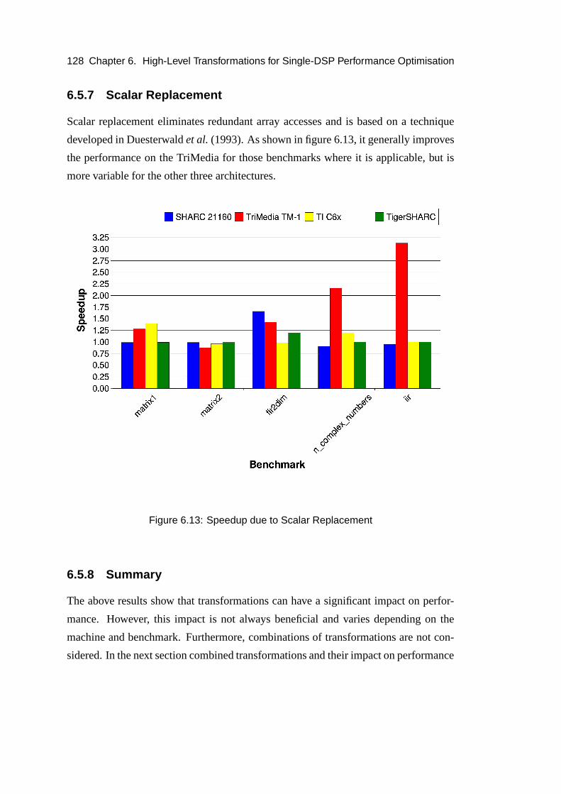
128 Chapter 6. High-Level Transformations for Single-DSP Performance Optimisation
6.5.7 Scalar Replacement
Scalar replacement eliminates redundant array accesses and is based on a technique
developed in Duesterwald et al. (1993). As shown in figure 6.13, it generally improves
the performance on the TriMedia for those benchmarks where it is applicable, but is
more variable for the other three architectures.
Figure 6.13: Speedup due to Scalar Replacement
6.5.8 Summary
The above results show that transformations can have a significant impact on perfor-
mance. However, this impact is not always beneficial and varies depending on the
machine and benchmark. Furthermore, combinations of transformations are not con-
sidered. In the next section combined transformations and their impact on performance

6.6. Iterative Search 129
are investigated.
6.6 Iterative Search
Most optimising compilers perform their transformations based on static program anal-
yses without incorporating feedback on the effectiveness of the applied transforma-
tions. Many of those compilers even perform a fixed sequence of transformations in
a static order. The reason for choosing such an approach is its low complexity. In the
general-purpose computing domain, it is often not desirable to let the compiler search
for an optimal transformation sequence for a program that takes just seconds to ex-
ecute even without any optimisations. In the DSP domain, however, the situation is
very different. Highly specialised processors perform time-critical tasks over and over
again, so that code performance is paramount. To a certain extent, increased compila-
tion and optimisation times are acceptable if the resulting code performs significantly
better than codes produced by standard compilation techniques. Based on this obser-
vation, an iterative feedback-driven approach to DSP high-level code transformation is
presented in this section.
6.6.1 Iterative Optimisation Framework
In figure 6.14 an overview of an iterative compilation and optimisation framework is
given. C source code enters the system and is translated into an Intermediate Represen-
tation (IR) by the front-end. The generated IR must be suitable to express high-level C
constructs such that a later stage can convert this IR back to C. The IR is then passed
on to a Transformation Engine. This transformation engine is driven by an Optimi-
sation Engine and fetches its Transformation Rules from an attached Transformation
Database. The transformation engine applies a transformation as directed by the op-
timisation engine to its input and passes the transformed program on to a C Code
Generator. This module translates the IR back to C code, which is then in turn fed into
an existing C compiler and linker for the target architecture. Linker information such
as the memory footprint of the compiled program is passed back to the optimisation
engine, which decides on the further optimisation strategy based on this and additional

130 Chapter 6. High-Level Transformations for Single-DSP Performance Optimisation
timing information gathered from profiled program execution.
Figure 6.14: Overview of the iterative compilation/optimisation framework
The implementation uses the infrastructure provided by the Stanford SUIF com-
piler (front-end, IR-to-C translator, transformations) and the DSP manufacturers’ C
compilers and simulators. In the following section a simple, but effective implementa-
tion of the iterative search algorithm as used in the optimisation engine of figure 6.14
is described.
6.6.2 Iterative Search Algorithm
For all but very small sets of transformations it is impossible to perform an exhaustive
search of all possible transformation sequences and parameters. Any practical search
algorithm must therefore trade in some “accuracy” for better runtime, i.e. it might not
find the optimal, but a sufficiently “good” solution in acceptable time.
6.6. Iterative Search 131
The iterative search algorithm employed in this work is based on following heuris-
tic principle: Individual transformations are explored first in isolation, then “success-
ful” candidates are concatenated to obtain potentially better combined transformation
sequences. Transformations are grouped in three categories according to their effect
on further transformations. Enablers are transformations that do not necessarily im-
prove a program’s performance on their own, but enable other performance-enhancing
transformations. Performers are the actual performance increasing transformations,
and Adaptors are transformations that are usually applied very late in a sequence of
transformations. Adapters usually adapt a program to a specific compiler or architec-
ture. Examples of enablers are pointer conversion and delinearisation, whereas loop
unrolling and scalarisation are examples of performers. The opposite of pointer con-
version, i.e. the conversion of array expressions into pointers (Liem et al., 1996), or
the substitution of specific patterns of C code with more efficient non-standard built-in
functions (Bodin et al., 1998) belong to the class of the adaptors. This search strategy
does not always find an optimal solution, but in practice it has proven to find good
solutions in reasonable time.
Different search strategies have been investigated by other researchers. In Fursin
et al. (2002), a random search strategy for numerical Fortran algorithms is evaluated,
and Falk (2001) proposes neural network based search and optimisation, but without
giving empirical results. Since the main goal of this work is to provide evidence of the
effectiveness of high-level transformations in the DSP domain, a simple, but effective
search algorithm has been chosen.
In figures 6.15 to 6.16 the iterative search algorithm is presented. The algorithm
maintains a working list L which initially only contains the original program. Itera-
tively enablers and a randomly selected performer are applied to member of the work-
ing list. The resulting program is stored back to the working list after transformation.
Results of enablers are always added to the working list, while programs transformed
by performers are only considered if their performance has been improved. After a pre-
defined number of iterations, this process terminates and the best program is selected
for further post-processing.
More formally, the algorithm can be described as follows. Let T = {T1,T2, . . . ,Tn}

132 Chapter 6. High-Level Transformations for Single-DSP Performance Optimisation
be a set of transformations and TE (Enablers), TP (Performers) and TA (Adaptors) dis-
tinct subsets of T such that TE ⊂ T , TP ⊂ T , TA ⊂ T and TE ∪ TP ∪ TA = T . A
transformation Tk is a function Tk : P×� n −→ P taking a program p ∈ P , where P is
the set of all programs, and n integer parameters2. Tk produces a transformed program
p′ ∈ P as its result.
6.7 Results and Analysis
Since the main focus of high-performance signal processing is on runtime perfor-
mance, emphasis during benchmarking is on execution time speedup. Code size and
power consumption are important constraints but are beyond the scope of this thesis.
Nonetheless, fixed memory size has been considered and restricts the legality of certain
transformations.
6.7.1 Benchmark-oriented Evaluation
In figure 6.17, the results for the selected set of benchmarks are summarised. For each
benchmark program and each architecture the maximum speedup achieved is shown.
Figure 6.18 lists the transformations needed to obtain these speedups.
Highlighting the best performance is justified by the fact that an expert programmer
or a feedback-directed compiler tries several different options before selecting the best
one.
6.7.1.1 matrix1
The matrix1 benchmark computes the product of two matrices. After pointer con-
version of the original program several different transformations and analyses can be
applied to this program. For the ADSP-21160 delinearisation and subsequent SIMD-
style parallelisation result in a speedup of 5.48. The transformed program utilises both
2In the interest of a simpler presentation, transformations are restricted to those with integer param-eters. This, however, does not restrict the generality of the presented iterative search algorithm, whichcan be easily extended to more general parameters of different types

6.7. Results and Analysis 133
Input: Program pin ∈ P , Bound B ∈ �Output: Program pout ∈ P
1. Measure baseline case.
Execute & profile pin;
tbaseline = time(pin);
2. Optimisation space exploration.
working list L = {(pin, tbaseline)};
steps = 0;
While (steps < B) Do
Select p ∈ L;
For all t ∈ TE
If t applied to p is legal Then
insert t(p) to L;
Select randomly t ∈ TP
If t applied to p is legal Then
Select r ∈ � n
Execute & profile tr(p);
If time(tr(p)) < time(p) Then
insert (tr(p), time(tr(p))) to L;
EndIf
steps = steps+1;
EndWhile
3. Machine and compiler specific post-processing.
Select program p ∈ L with minimal runtime tmin
Apply post-processing algorithm to p (see figure 6.16)
4. Output.
Return program p.
Figure 6.15: Iterative search algorithm for exploring the high-level transformation space

134 Chapter 6. High-Level Transformations for Single-DSP Performance Optimisation
Input: Program pin with runtime timein.
Output: Program pout with runtime timeout .
timemin = timein;
pmin = pin;
Select transformation t ∈ TA and parameters r ∈ � n
If tr is applicable and legal Then
p′ = tr(pmin);
Execute & profile p’;
if time(p′) < tmin then
pmin = p′;
tmin = time(p′);
Return (pmin, tmin)
Figure 6.16: Machine and compiler specific post-processing
datapaths of the Analog Devices processor and also its two memory banks can be used
in parallel, whereas the original program makes poor usage of the available resources.
The TriMedia benefits most from a delinearised version of the array-based program
to which scalarisation, loop unrolling and padding have been applied. Each transfor-
mation applied on its own already increases the performance, but in combination a
speedup of 3.82 can be observed. Loop unrolling increases the flexibility of the in-
struction scheduler to fill the five issue slots of the TM-1 with instructions since the
new loop body has more instructions to chose from. Scalarisation reduces the number
of memory accesses whereas padding reduces the number of cache conflicts. The situ-
ation is similar for the TI C6201 and the TigerSHARC, although the best performance
is achieved with just array recovery and loop unrolling together. The execution speed
can be more than doubled on the C6201 architecture, and increased by 37% on the
TigerSHARC.

6.7. Results and Analysis 135
Figure 6.17: Best overall performance for combined transformations

136 Chapter 6. High-Level Transformations for Single-DSP Performance Optimisation
BenchmarkArchitecture
SHARC 21160 TriMedia TM-1 TI C6201 TigerSHARC TS101
matrix1 PC,D,SIMD PC,D,S,P(1),U(9) PC,U(3) PC,U(6)
matrix2 (Original) PC,P(1),U(5),S PC,U(3) U(3)
matrix1x3 PC,U(total) PC,U(total) PC,U(total) U(2)
fir PC,SIMD(part.) PC,U(8) PC,U(15) PC,U(6)
fir2dim PC,S PC,D,S,U PC,S,U,AC PC,S,U(3)
convolution PC,SIMD U(10) U(8) (Original)
n real updates PC,SIMD PC,U(3) U(9) (Original)
n complex updates PC,SIMD(part.) PC,D,S,U(2) PC,D,S PC,U(6)
dot product (Original) PC,U(total) (Original) (Original)
iir biquad N sections PC,D,S PC,U(5) (Original) (Original)
lms PC,SIMD(part.) PC,U(11) PC,U(7) PC,U(6)
(PC = Pointer Conversion, U = Loop Unrolling (Factor), D = Delinearisation, P = Array Padding (Size), AC = Array Conversion)
Figure 6.18: Best transformation sequences for the DSPstone benchmark suite
6.7.1.2 matrix2
This program is based on the same matrix multiplication algorithm as matrix1, but in
this implementation the first and last iteration of the inner loop are peeled off. Origi-
nally intended as a hint to the compiler to create efficient code for the available AGUs
and to avoid the otherwise necessary accumulator clear operation before the loop, this
transformation prevents the exploitation of SIMD parallelism on the ADSP-21160.
Since the required double-word alignment of array data in SIMD loops is violated, the
matrix2 benchmark cannot take benefit of parallel loops unless it is “re-transformed”
back into the more regular form of matrix1. Still, pointer conversion and loop un-
rolling can be applied and yield a speedup of 1.16.
For VLIW architectures the situation is different. On the TriMedia a speedup of
3.52 can be achieved after array recovery, padding, scalarisation and 5-fold unrolling.
The TI DSP, unlike the SHARC, benefits from the differences of the matrix2 im-
plementation, after array recovery and 3-fold unrolling a speedup of 2.39 is possible.
6.7. Results and Analysis 137
This speedup mainly results from array recovery with unrolling contributing only a
small percentage. The inspection of the assembly code generated by the compiler re-
veals a more efficient inner loop due to a higher degree of instruction-level parallelism.
After array recovery the number of operations in the loop is not only smaller, but the
number of operations executed in parallel is higher. Explicit array accesses increase
the efficiency of the data dependence analysis supporting the compiler built-in software
pipelining transformation.
Unrolling can still improve the performance by 20% on the TigerSHARC. Never-
theless, the absolute performance of matrix2 does not reach that of matrix1 on this
architecture due to inferior data alignment.
6.7.1.3 matrix1x3
This program computes the matrix product of a 3× 3 matrix and a 3× 1 vector in a
simple loop with few iterations. For the ADSP-21160 array recovery and total loop
unrolling of the very small loop can speed up the execution by a factor of 1.93. The
largest speedup on the TriMedia can be achieved with total loop unrolling of either
the pointer or array-based version of the program. Although loop unrolling in general
increases the code size, it is well justified in this case as the loop iteration range as
well as the loop body are both very small. On the C6201 total loop unrolling of the
array-based code also can be accounted for the largest possible speedup, but the perfor-
mance gain on this architecture is smaller than on the TriMedia. On the TigerSHARC,
unrolling accounts for the largest performance improvement. Although padding helps
improve performance on its own, it does not contribute to any combined transforma-
tion. Several different unroll factors for the pointer as well as the array-based codes
yield the same maximal performance.
6.7.1.4 fir
This program is an implementation of a Finite Impulse Response (FIR) filter and con-
tains a single loop. After array recovery this loop is amendable to loop reversal and
loop splitting, before one of the resulting loops can be SIMD parallelised. After this
transformation, a speedup of 1.32 is achieved. Since the other loop contains a memory

138 Chapter 6. High-Level Transformations for Single-DSP Performance Optimisation
access to a non double-word aligned array element, this loop must be executed sequen-
tially. Further transformations in order to overcome this restriction are possible, but are
beyond standard compiler analysis. Loop unrolling of the array-based loop gives the
best results on the TriMedia and the TigerSHARC. 8-fold and 6-fold unrolling result in
speedups of 2.20 and 2.18, respectively. On the C6201 the same set of transformations
accounts for the largest speedup, which is 1.08. Again, the achieved speedup is smaller
on the TI processor than the TriMedia or the TigerSHARC.
6.7.1.5 fir2dim
This code is a two-dimensional FIR filter. In theory, the fir2dim benchmark could be
parallelised for the ADSP-21160, but the compiler is overly restrictive with the use of
the SIMD loop directive. In sequential execution mode, scalarisation can be applied
after array recovery of the program and a speedup of 1.66 is obtained. Unlike the other
programs where scalarisation cannot improve the performance, fir2dim benefits from
this transformation because it can be applied across the three inner loops where redun-
dant memory accesses are removed. The compiler is not able to remove these accesses
without this high-level code transformation. On the TriMedia a speedup of 7.38 is pos-
sible after array recovery, delinearisation, scalarisation and total unrolling of the three
small inner loops. Similarly, on the TigerSHARC a speedup of 2.95 can be realised by
pointer conversion, scalarisation and unrolling. For the C6201 a pointer-based version
of the program achieved the best performance, but only after it has been converted into
the array-based representation which allowed the application of array dataflow analy-
sis and scalarisation. After scalarisation and loop unrolling the program was converted
back into the pointer-based form which gave an overall speedup of 1.02. Although the
speedup is small, this example shows that it is possible to apply transformations that
could not be applied to the pointer-based program. In addition, it is possible to go back
to pointer-based code when this appears to improve the overall performance.
6.7.1.6 convolution
This convolution code can easily be parallelised for the ADSP-21160 after array recov-
ery and the execution time is reduced to 25.9% of the original time. For the TriMedia
6.7. Results and Analysis 139
10-fold loop unrolling does best, it results in a speedup of 3.56. Similarly, the largest
speedup on the C6201 is achieved with 8-fold unrolling. The increased size of the loop
body provides the TriMedia and TI compiler with an increased flexibility for instruc-
tion scheduling and reduces the number of NOP-operations. On the TigerSHARC the
unmodified, original program performs best.
6.7.1.7 n real updates
The main computational loop in this program can be easily parallelised for the ADSP-
21160 and a speedup of 3.91 is achieved. The TriMedia benefits most from pointer
conversion and unrolling. Array recovery helps the compiler to prove independence
of different memory accesses, whereas loop unrolling increases the number of instruc-
tions in the loop body. The maximum speedup achievable on the TriMedia is 3.78.
However, the maximum speedup on the C6201 is rather small, 1.02, and due to 9-
fold loop unrolling of the pointer-based code. Again, on the TigerSHARC the original
program exhibits the best performance.
6.7.1.8 n complex updates
Full SIMD parallelisation fails due to an overly restrictive compiler, but it is still pos-
sible to take advantage of the two functional units of the ADSP-21160 after array
recovery, loop splitting and parallelisation of one of the resulting loops. For the Tri-
Media array recovery once again was proven to be useful supporting other transforma-
tions such as delinearisation and scalarisation. Together with 2-fold loop unrolling, a
speedup of 2.52 was obtained. The same set of transformations but without unrolling
also achieved the largest speedup on the C6201. The TigerSHARC benefits most of
pointer conversion and 6-fold loop unrolling.
6.7.1.9 dot product
The original pointer-based program performs best on the ADSP-21160. SIMD par-
allelisation is applicable, but the overhead involved in switching from sequential to
SIMD mode and back is larger than the benefit obtained from parallel processing.

140 Chapter 6. High-Level Transformations for Single-DSP Performance Optimisation
Also loop unrolling is not beneficial as it increases the execution time. In contrast,
loop unrolling of either the pointer or array-based program results in a speedup of 4.6
on the TriMedia. This VLIW architecture clearly benefits and can take advantage of
the removal of the loop construct during instruction scheduling. The original loop with
just two iterations causes many NOP operations and branch penalties, which can be
eliminated by complete unrolling. The TI compiler handles the loop as well as the
unrolled straight-line code, so the runtime of the original program cannot be improved
by unrolling. The same is true for the TigerSHARC.
6.7.1.10 iir biquad N sections
This is a benchmark that implements an Infinite Impulse Response (IIR) filter with
N biquad sections. SIMD parallelisation cannot be applied to this program due to a
loop-carried data dependence in its loop body. However, the sequential version for the
ADSP-21160 can be improved by array recovery, delinearisation and scalarisation giv-
ing a speed up to a factor of 1.14. Array recovery and 5-fold unrolling gives the best
performance with a speedup of 4.41 on the TriMedia. An inspection of the compiler
generated assembly code shows a much tighter packing of operations into machine
instructions, i.e. the number of wasted issue slots filled with NOPs is significantly re-
duced. Experiments on the C6201 were less successful due to technical problems with
this program in the available simulation environment. However, initial results show
only small chances of achieving a significant speedup due to a good performance of
the original code. Once again, the TigerSHARC compiler produces the best perform-
ing executable from the unmodified, i.e. original source code.
6.7.1.11 lms
lms is the kernel of a Least Mean Square (LMS) filter. The lms program contains two
loops that can both benefit from SIMD parallelisation. After array recovery, loop rever-
sal is applicable, so that the Analog Devices compiler accepts the first loop as a SIMD
loop. An overall speedup of 1.70 is achieved on the ADSP-21160. The TriMedia, the
C6201 and also the TigerSHARC architecture benefit most from array recovery and
loop unrolling and speedups of 3.16, 1.56, and 2.70, respectively, are possible.

6.7. Results and Analysis 141
6.7.2 Architecture-oriented Evaluation
Overall the TriMedia benefits the most from high-level transformations with an av-
erage speedup of 3.69, the C6201 the least with a speedup of 1.39 and the SHARC
and TigerSHARC somewhere in between with an average speedups of 2.31 and 1.57,
respectively.
6.7.2.1 TriMedia
In all but one case, the best optimisation for each program required pointer to array
conversion. This alone can improve performance on the TriMedia as can be seen in
figure 6.6. The most important benefit of pointer conversion, however, is that it en-
ables further transformations such as delinearisation, padding and scalar replacement.
Although unrolling was useful in all cases, it required additional transformations in all
bar one case to give the best performance. The TriMedia, in general, benefited most
from the application of combined transformations. This is mainly due to its more com-
plex architecture, in particular the combination of a 5-way VLIW processor and an
on-chip cache. Finally, the success of high-level transformations on the TriMedia are
also in part due to its relatively immature compiler.
6.7.2.2 TI C6201
The C6201 benefits least of all from the application of high-level transformations. Yet
even with a mature native compiler, it is possible to get on average a speedup of 1.39. In
all but four cases pointer to array conversion was required to get the best performance,
two of those cases being when no optimisation gave any improvement. Unrolling was
once again useful in exposing ILP especially when combined with pointer to array
conversion. Unlike the TriMedia, shorter transformation sequences seemed to perform
best. The C6201 rarely benefited from scalar replacement as the native compiler was
largely capable of detecting redundant memory accesses in all but two cases.
142 Chapter 6. High-Level Transformations for Single-DSP Performance Optimisation
6.7.2.3 SHARC
The SHARC experiences the highest speedup when its SIMD capabilities can be ex-
ploited. Although pointer to array conversion always degrades performance in iso-
lation, when combined with SIMD vectorisation it provides significant performance
improvement. Overly restrictive requirements on the pragma directive prevented fuller
exploitation of the SHARC SIMD capabilities.
6.7.2.4 TigerSHARC
Although the TigerSHARC bears some similarity to its predecessor, the Analog De-
vices SHARC, it responds very differently to high-level transformations. The maturer
compiler does not expect the programmer to indicate the usage of SIMD parallelisation
any more, but performs this task automatically. Pointer conversion still is an impor-
tant transformation that either enables other high-level transformation or supports the
manufacturer’s compiler. All but four programs significantly gain performance from
combined transformations with pointer conversion and loop unrolling being the most
effective ones.
6.7.2.5 Summary
Overall, selecting the appropriate high-level transformation gives on average a 2.21
speedup across the four platforms investigated. In 31 out of 44 cases, pointer to array
conversion contributes to the increased performance and in only three cases the best
performance was gained with transformations other then pointer to array conversion.
6.8 Related Work and Discussion
There has been little work in evaluating the impact of transformation sequences on
real DSP processors. In Andreyev et al. (1996) a heuristic optimisation method is
presented that strongly relies on the information of how a certain compiler for a specific
processor exploits high-level program constructs for code generation. This approach is
very restricted in the sense that it cannot be easily transferred to a different processor or

6.8. Related Work and Discussion 143
even a different compiler for the same processor. Although aimed at DSP applications
the authors only present few results for a general-purpose processor (Intel Pentium).
An address optimisation based on a sequence of source-to-source transformations
is shown and evaluated in Gupta et al. (2000). This optimisation relies on explicit array
accesses and does not work with pointer-based programs. Here the pointer-conversion
algorithm can be applied as a preparatory stage that enables the further optimisation.
Although aiming at DSP applications the experimental results come from general-
purpose CPUs. It is not at all obvious if the transformation extends to DSPs as the
authors claim, and a demonstration of this is still outstanding.
Software pipelining as a source-to-source transformation in the context of DSP ap-
plications is investigated in Wang and Su (1998) and Su et al. (1999). The combined
effect of different optimisations is neglected apart from two normalisation transfor-
mations (renaming and loop distribution) needed by this approach. The evaluation of
the effectiveness of the presented transformation is performed on a single architecture
(Motorola DSP56300) where it achieved good results, albeit for a small set of bench-
mark programs.
The effect of unroll-and-jam and scalar replacement for imperfectly nested loops is
evaluated in Song and Lin (2000). A simple heuristic method is used to determine the
unroll factor and the results are compared with strip-mining, loop distribution and loop
unrolling. The SC140 processor serves as the target architecture for the experimental
evaluation. The results are promising, although the number of benchmark programs is
very small and only a single architecture has been considered.
One of the main reasons that there has been little evaluation of transformation
sequences is due to the pointer-based nature of many of the benchmarks. The pointer
conversion algorithm developed in this thesis allows for an efficient reconstruction of
explicit array accesses and enables many further transformations.
In this chapter it has been demonstrated that combining array recovery and high-
level transformations can lead to excellent single-processor performance. However,
finding a “good” transformation sequence is a difficult task. There has been much
work investigating the use of static analysis to determine the best transformation order
(Kandemir et al., 1999). This approach is highly attractive in the context of general-

144 Chapter 6. High-Level Transformations for Single-DSP Performance Optimisation
purpose computing as the analysis is typically a small fraction of the compilation time.
Transformation selection based on static analysis is a fast, but unfortunately frequently
inaccurate approach. Feedback-directed approaches have proved promising where ac-
tual runtime data is used to improve optimisation selection.
In the OCEANS project (Barreteau et al., 1998) high and low-level optimisations
within an iterative compilation framework for embedded VLIW processors were inves-
tigated. Experimental results for the TriMedia TM-1000 show that such an approach
has promise. More recently, the use of iterative compilation has been further investi-
gated, where different optimisations are selected and evaluated, with the eventual best
performing one selected (Kisuki et al., 2000). Such an approach has a much longer
compilation time, but this is not a major issue in embedded systems. Using such an
approach, a compiler can automatically find the best speedups shown in figure 6.17.
6.9 Conclusion
In this chapter, empirical evidence of the usefulness of the application of high-level
transformations to DSP applications has been given. The evaluation considers four dif-
ferent embedded platforms. Selecting the appropriate transformation using an iterative
transformation framework gives on average a 2.21 speedup across the four platforms
investigated. The programs considered are relatively straightforward kernels and fu-
ture work will investigate larger applications to determine where the potential scope
for high-level optimisations is even greater.
Key enabler of most of evaluated high-level transformations is the pointer conver-
sion transformation developed in chapter 5.1.
Given the empirical evidence justifying the use of high-level transformations, a
compiler strategy exploiting such transformations is proposed. An iterative approach to
optimisation selection has been investigated, implemented and found useful in practice.
Future work will consider the integration of high-level optimisation with low-level
code selection and scheduling, as well as more advanced search strategies.

Chapter 7
Parallelisation for Multi-DSP
Multi-processor DSPs offer a cost-effective method of achieving high performance
which is critical for many embedded application areas. However, porting existing uni-
processor applications to such parallel architectures is currently complex and time-
consuming. There are no commercially available compilers that will take existing
sequential DSP programs and map them automatically onto a multi-processor machine
(Rijpkema et al., 1999). Instead, users are typically required to rewrite their code as a
process network or a set of communicating sequential processes (Lee, 1995) . Such an
approach is well known to be highly non-trivial and error-prone, possibly introducing
deadlock.
Rewriting an application in a parallel manner is a highly specialised skill. What
is needed is a tool that takes existing programs and maps them automatically onto the
new multi-processor architecture efficiently. Although there has been over 20 years
of research into auto-parallelising compilation in scientific computing (Gupta et al.,
2000), this has not taken place in the embedded domain. This is due to two main rea-
sons: (i) DSP programs are written in C rather than Fortran (Hiranandani et al., 1992)
and make extensive use of pointer arithmetic and (ii) the distributed memory space of
multi-processor DSPs is difficult to compile for. These two problems are approached
by using the pointer conversion technique developed in section 5.1 and a new address
resolution technique, based on a novel data transformation scheme, that allows par-
allelisation for multiple address spaces without introducing complex (and potentially
deadlocking) message passing code. By embedding these two techniques into an over-
145

146 Chapter 7. Parallelisation for Multi-DSP
all parallelisation strategy, an auto-parallelising C compiler for DSP applications that
outperforms existing approaches has been developed.
This chapter is structured as follows. Section 7.1 provides a motivating example
and is followed in section 7.2 by a description of the auto-parallelisation scheme. Sec-
tion 7.3 describes the approach to partitioning in detail, and in section 7.4 a new data
address resolution technique is introduced. A larger example is given in section 7.5.
This is followed by a short review of related work in section 7.6 and some concluding
remarks in section 7.7.
7.1 Motivation & Example
Auto-parallelising compilers that take as input sequential code and produce parallel
code as output have been studied in the scientific computing domain for many years.
In the embedded domain, multi-processor DSPs are a more recent compilation target.
At first glance, DSP applications seem ideal candidates for auto-parallelisation; many
of them have static control-flow and linear accesses to matrices and vectors. However,
auto-parallelising compilers have not been developed due to the widespread practice of
using post-increment pointer accesses (Zivojnovic et al., 1994). Furthermore, multi-
processor DSPs typically have distributed address spaces removing the need for expen-
sive memory coherency hardware. This saving at the hardware level greatly increases
the complexity of the compiler’s task.
7.1.1 Memory Model
This work exploits the fact that although multi-processor DSP machines typically have
multiple address spaces, part of each processor’s memory space is visible from other
processors, unlike pure message-passing machines. However, unlike single address
space machines, a processor must know both the identity of the remote processor and
the location in memory of the required data value. For example, figure 7.21 shows
the global memory map of a multi-processor system comprising the Analog Devices
TigerSHARC processor. Each processor has its internal address space for accesses to
1Identical to figure 3.7 in chapter 2.2.

7.1. Motivation & Example 147
Original Code (1) Pointer Conversion (2)
for (i = 0 ; i <=15 ; i++)
*p_d++ = *p_c++ + *p_a++ * *p_b++ ;
for (i = 0 ; i <=15 ; i++)
D[i] = C[i] + A[i] * B[i] ;
Partitioned Data (3) Address Resolution(4)
#define z 0
for (i = 0; i<=7; i++)
D[z][i] = C[z][i] + A[z][i] * B[z][i];
#define z 0
int D0[8]; /* local */
extern int D1[8]; /* remote */
int *D[2] ={D0,D1};
for (i = 0; i<=7; i++)
D[z][i] = C[z][i] + A[z][i] * B[z][i];
Figure 7.1: Example showing partitioning and translation scheme
local data. These accesses are purely local and not reflected on the external bus. In
addition, the processors’ memories form a global address space where each processor
is assigned a certain range of addresses. This global address space is used for bus-
based accesses to remote data where the global address (or equivalently the remote
processor’s identity and the data’s local address) must be known.
A novel technique which combines single-address space parallelisation approaches
with a novel address resolution mechanism has been developed. For linear accesses,
it determines at compile time the processor and memory location of all data items.
Non-linear accesses are resolved during runtime by means of a simple descriptor data
structure.
7.1.2 Example
The example in figures 7.1 and 7.3 illustrates the main points of this chapter. The
code in figure 7.1, box (1) is typical of C programs written for DSP processors; it is

148 Chapter 7. Parallelisation for Multi-DSP
Figure 7.2: TigerSHARC global memory map (Analog Devices, 2001a)
part of the n real updates routine from the DSPstone benchmark suite. The use of
post-increment pointer traversal is a well know idiom (Zivojnovic et al., 1994). This
form, however, will prevent many optimising compilers from performing aggressive
optimisation and will prevent attempts at parallelisation. The second box (2) in figure
7.1 shows the program after pointer conversion.
Figure 7.3(a) presents a diagram showing the corresponding data layout of one of
the arrays, D. The pointers are replaced with array references based on the loop iterator.
SPMD owner-computes parallelisation based on data and computation partitioning and
distribution across the processor nodes is straightforward here. There is just one array
dimension and one loop, both of which are partitioned by the number of processors.
In this example, it is assumed there are two processors. Partitioning is achieved by
strip-mining (O’Boyle and Knijnenburg, 2002) each array to form a two-dimensional
array whose inner index corresponds to the two processors. For instance, the array D
is now partitioned such that D[0][0...7] resides on processor 0 and D[1][0...7]

7.1. Motivation & Example 149
Figure 7.3: Data layout for figure 7.1
resides on processor 1. The iterator is similarly partitioned to iterate over the work
allocated to it, 0 . . .7. The partitioned code for processor 0 (as specified by z) is shown
in figure 7.1, box (3). The code for processor 1 is identical except for #define z 1.
The diagram in figure 7.3(b) illustrates the new data layout for array D, where each row
of the strip-mined array resides on a separate processor.
Although there are other methods of partitioning code and data, this approach al-
lows for a simple translation to multiple address spaces. In fact, for single address
space machines, this would be sufficient. However, the programming model of multi-
DSPs requires remote, globally-accessible data to have a distinct name to local data2.
Thus, each of the sub-arrays are renamed: D[0][0...7] becomes D0[0...7] and
D[1][0...7] becomes D1[0...7]. On processor 0, D0 is declared as a variable re-
siding on that processor while D1 is declared extern. For processor 1, the reverse
declaration is made, i.e. D0 is extern.
2Otherwise they are assumed to be private copies.

150 Chapter 7. Parallelisation for Multi-DSP
To access both local and remote data, a local pointer array is set up on each pro-
cessor (see box (4) of figure 7.1). The array contains two pointer elements (as two
processors are assumed), which are assigned to the start address of the local arrays
on the two processors. The original name of the array D[][] is used as the name of
pointer array *D[] Then, this array is initialised to point to the two distributed arrays
int *D[2] = {D0,D1}. This is shown diagrammatically in figure 7.3(c). Using the
original name means that exactly the same array reference form in all uses of the ar-
ray D as in the single address case can be used. Hence, the array references shown in
figure 7.1, box(4), have not changed. This has been achieved by using the fact that
multi-dimensional arrays in C are arrays of arrays and that higher dimensions arrays
are defined as containing an array of pointers to sub-arrays3. From a code generation
point of view this greatly simplifies implementation and avoids complex and difficult
to automate message passing.
7.2 Parallelisation
The overall parallelisation algorithm is shown in figure 7.4. Pointer to array conversion
is first applied to enable data dependence analysis. Once the program is in a pointer-
free form, standard data dependence analysis is applied to determine if the program
is parallel and if so, a check to see if the amount available justifies parallelisation4 is
applied.
7.3 Partitioning and Mapping
Data parallelism in DSP programs is exploited by partitioning data and computation
across the processors using an owner-computes, SPMD model of computation. Choos-
ing the best data partition has been studied for many years (Lim et al., 1999) and is
NP-complete. In this work, a simple method exploiting parallelism and reducing com-
munication is used; more advanced partitioning schemes, e.g. affine partitioning (Lim
3As defined in section 6.5.2.1 of the ANSI C standard paragraphs 3 and 4.4Currently, the parallelised loop trip count is multiplied by the number of operations and checked
whether it is above a certain threshold before continuing.

7.3. Partitioning and Mapping 151
1. Convert pointers to arrays
2. IF pointer free THEN perform data dependence analysis
(a) IF parallel and worthwhile
i. Determine data partition
ii. Partition + transform data and code
iii. Perform address resolution
3. Parallel Code Generation
Figure 7.4: Overall parallelisation algorithm
et al., 1999), could also be used instead. The key point here is that the partitioning
and mapping approach makes the processor identifier explicit, which is exactly what is
needed to statically determine whether data is local or remote.
7.3.1 Notation
Before describing the partitioning and mapping approach, the notation used is briefly
described. The loop indices or iterators can be represented as an M×1 column vector
III = [i1, i2, . . . , iM]T where M is the number of enclosing loops. The loop ranges can
be described by a system of inequalities defining the polyhedron or iteration space
BIII ≤ bbb, where B is a (`×M) integer matrix and bbb a (`× 1) vector. The data storage
of an array A can also be viewed as a polyhedron. Formal indices JJJ = [ j1, j2, . . . , jN]T
are introduced, where N is the dimension of array A, to describe the array index space.
This space is given by the polyhedron AJJJ ≤ aaa, where A is a (2N×N) integer matrix
and aaa a (2N× 1) vector. It is assumed that the subscripts in a reference to an array
A can be written as UIII + uuu, where U is a (N×M) integer matrix and uuu is a (N× 1)
vector.

152 Chapter 7. Parallelisation for Multi-DSP
7.3.2 Partitioning
Data arrays are partitioned along those dimensions of the array that may be evaluated
in parallel and minimise communication. Determining those index dimensions that
may be evaluated in parallel, in general, gives a number of options and, therefore, a
simple technique to reduce communication based on data alignment is used.
If two array references have every element in a certain dimension corresponding
to the same index space points then they are aligned. i.e. a[i][j] and b[i][k] are
aligned on the first index but not on the second. If two arrays are aligned with respect to
a particular index, then no matter how those individual array elements are partitioned,
any reference with respect to this index will always be local. Partitioning based on
alignment tries to maximise the rows that are equal in a subscript matrix.
Let δ(x,y) be defined as follows:
δ(x,y) =
{
1 x = y∧ x 6= 0
0 otherwise(7.1)
This function determines whether two subscripts are non-zero and equal. The function
H(i) defined as:
H(i) = ∑t
δ(U1i ,Ut
i ) (7.2)
which measures how well a particular index i of an array use, U t , is aligned with the
array definition, U1. For each index the value of H is calculated, the index with the
highest value being the one to partition along.
This technique is applied across all statements and in general there will be conflict-
ing partition requirements. Currently, only those statements in the deepest nested loops
are considered as they dominate execution time and calculate the value of H across all
these statements for different parallel indices i. The index with highest value for H,
imax,H , determines the index to partition along.
A partition matrix P is constructed:
Pi =
{
eTi if i = imax,H
0 otherwise
}
(7.3)

7.3. Partitioning and Mapping 153
where eTi is the ith row of the identity matrix Id . Also a sequential matrix S containing
those indices not partitioned such that P +S = Id is constructed.
Original Code (1) Partitioned Code and Data (2) Address Resolution(3)
int y[32][32];
for (i=0; i<32; i++)
for (j=0; j<32; j++)
y[i][j]=a[i][j]
* h[31-i][j];
int y[4][8][32];
for(z=0; z<4; z++)
for (i=0; i<8; i++)
for (j=0; j<32; j++)
y[z][i][j]=a[z][i][j]
* h[3-z][7-i][j];
#define z 0
int y0[8][32];
extern int y1[8][32],
y2[8][32],
y3[8][32];
int *y[4] ={y0,y1,y2,y3};
for (i=0; i<8; i++)
for (j=0; j<32 ; j++)
y[z][i][j]=a[z][i][j]
* h[4-z][8-i][j];
Figure 7.5: Partition and translation with communication of array h
In the example in figure 7.5, box(1), H(0) = 1,H(1) = 2, imax,H = 1 and therefore
P =
[
0 0
0 1
]
and S =
[
1 0
0 0
]
(7.4)
7.3.3 Mapping
Once the array indices to partition along have been determined, strip-mining the in-
dices J based on the partition matrix P and strip-mine matrix Sp produces the new
domain J ′ where Sp is defined as
Sp =
[
(.)p
(.)%p
]
(7.5)
and p is the number of processors. Embedding of Sp produces a generalised strip-
mine matrix S . For further details see O’Boyle and Knijnenburg (2002). Let T be the

154 Chapter 7. Parallelisation for Multi-DSP
mapping transformation where
T = PS +S (7.6)
Thus the partitioned indices are strip-mined and the sequential indices left unchanged.
The new indices are given by
JJJ′′′ = TJJJ (7.7)
The new array bounds are then found:[
T O
O T
]
AT−1JJJ′′′ ≤
[
T O
O T
]
aaa (7.8)
and array accesses are updated accordingly
U′ = TU (7.9)
In general, without any further loop transformations, this will introduce mods and
divs into the array accesses. However, by applying a suitable loop transformation, in
this case T , this can be recovered.
Applying T to the enclosing loop iterators and updating the access matrices gives
III′′′ = T III (7.10)
where[
T O
O T
]
BT−1III′′′ ≤
[
T O
O T
]
bbb (7.11)
and
U′′ = TUT−1 (7.12)
7.3.4 Algorithm
In figures 7.6 and 7.7 detailed step-by-step descriptions of the proposed partitioning
and mapping algorithms are presented. They can be directly implemented in any
framework that supports extended matrices as introduced in O’Boyle and Knijnenburg
(2002).
Whereas the partitioning algorithm in figure 7.6 is independent of the specific target
architecture and computes the most suitable array index to partition along, the mapping
algorithm in figure 7.6 requires the number of processors to be known.

7.3. Partitioning and Mapping 155
1. Computation of alignment H(i) for all statements in the innermost loop body and all
indices i.
H(i) = ∑t
δ(U1i ,Ut
i )
2. Determination of imax,H .
Determine imax,H ∈ {i|∀ j : H(i)≥ H( j)}.
3. Construction of partition matrix P .
P =
{
eTi if i = imax,H
0 otherwise
}
where eTi is the ith row of the identity matrix Id .
4. Construction of sequential matrix S.
S = Id−P
Figure 7.6: Partitioning Algorithm

156 Chapter 7. Parallelisation for Multi-DSP
1. Construction of the Transformation Matrix T .
(a) Construction of the Strip-Mine Transformation Matrix
Sp =
[
(.)/p
(.)%p
]
and its Pseudo-Inverse
S†p =
[
p 1]
where p is the number of processors.
(b) Construction of the Generalised Strip-Mining Matrix S and its Pseudo-Inverse S †
S =
Id k−1 0 0
0 Sl 0
0 0 IdN−k
and S† =
Id k−1 0 0
0 S†l 0
0 0 IdN−k
(c) Construction of the Transformation Matrix T .
T = PS +S
2. Computation of new Array Index Space.
(a) Computation of new Array Indices JJJ′′′.
JJJ′′′ = T JJJ
(b) Computation of new Array Bounds A′JJJ′′′ ≤ aaa′′′.
[
T O
O T
]
AT−1JJJ′′′ ≤
[
T O
O T
]
aaa
3. Computation of new Iteration Space and Loop Bounds
(a) Computation of new loop iterators III′′′.
III′′′ = T III
(b) Computation of new loop bounds B ′III′′′ ≤ bbb′′′.
[
T O
O T
]
BT−1III′′′ ≤
[
T O
O T
]
bbb
4. Update of Array References U ′′III′′′+uuu.
Update all array references U ′′ = U′T−1 = TUT−1.
Figure 7.7: Mapping Algorithm
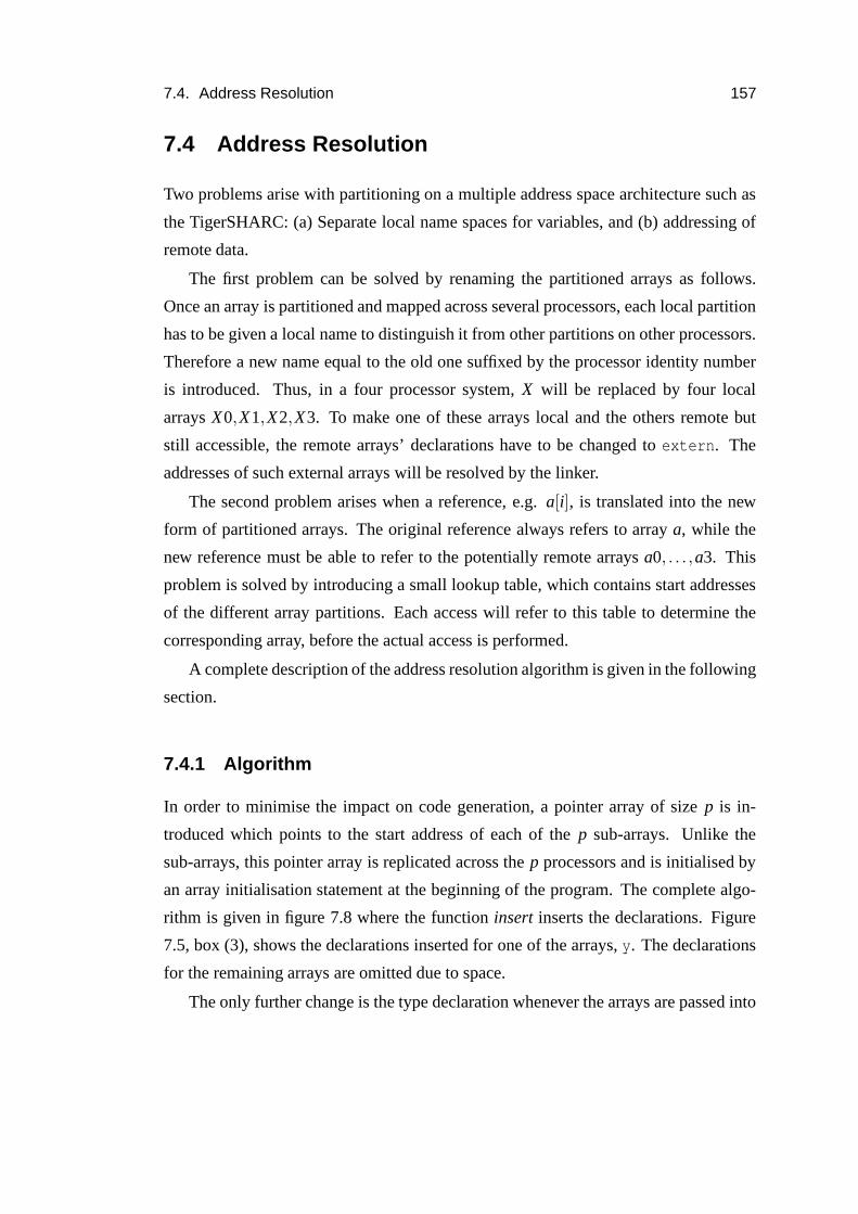
7.4. Address Resolution 157
7.4 Address Resolution
Two problems arise with partitioning on a multiple address space architecture such as
the TigerSHARC: (a) Separate local name spaces for variables, and (b) addressing of
remote data.
The first problem can be solved by renaming the partitioned arrays as follows.
Once an array is partitioned and mapped across several processors, each local partition
has to be given a local name to distinguish it from other partitions on other processors.
Therefore a new name equal to the old one suffixed by the processor identity number
is introduced. Thus, in a four processor system, X will be replaced by four local
arrays X0,X1,X2,X3. To make one of these arrays local and the others remote but
still accessible, the remote arrays’ declarations have to be changed to extern. The
addresses of such external arrays will be resolved by the linker.
The second problem arises when a reference, e.g. a[i], is translated into the new
form of partitioned arrays. The original reference always refers to array a, while the
new reference must be able to refer to the potentially remote arrays a0, . . . ,a3. This
problem is solved by introducing a small lookup table, which contains start addresses
of the different array partitions. Each access will refer to this table to determine the
corresponding array, before the actual access is performed.
A complete description of the address resolution algorithm is given in the following
section.
7.4.1 Algorithm
In order to minimise the impact on code generation, a pointer array of size p is in-
troduced which points to the start address of each of the p sub-arrays. Unlike the
sub-arrays, this pointer array is replicated across the p processors and is initialised by
an array initialisation statement at the beginning of the program. The complete algo-
rithm is given in figure 7.8 where the function insert inserts the declarations. Figure
7.5, box (3), shows the declarations inserted for one of the arrays, y. The declarations
for the remaining arrays are omitted due to space.
The only further change is the type declaration whenever the arrays are passed into

158 Chapter 7. Parallelisation for Multi-DSP
1. For each program qi ∈ 1, . . . p
(a) For each arrayName
i. For j ∈ 1, . . . , p
A. IF ( j 6= i) THEN insert (extern)
B. insert(TYPE arrayName j[N/p];)
ii. insert (TYPE *arrayName[p] = ()
iii. For j ∈ 1, . . . , p−1
A. insert (arrayName j ,)
iv. insert (arrayNamep ,);)
Figure 7.8: Address Resolution Algorithm
function. The type declaration is changed from int[][] to *int[] and this must be
propagated interproceduraly. Once this has been applied no further transformation or
code modification is required.
7.4.2 Synchronisation
It is beyond the scope of this thesis to describe synchronisation placement, though this
is essential for correct execution. All cross-processor dependences are marked and a
graph based algorithm is used to insert the minimal number of barrier synchronisations
(Tseng, 1995; Han and Tseng, 1998).
7.5 Example
In this section, a demonstration of the previously developed algorithm is given for a
larger example. Starting with the array recovered and delinearised matrix1 program
from the DSPstone benchmark suite, all parallelisation steps are shown. The resulting
parallel program can be either run directly, or further optimised (e.g. access localisa-
tion or single-processor optimisations).

7.5. Example 159
7.5.1 Sequential program
Figure 7.9 shows the sequential matrix1 program after pointer conversion and delin-
earisation. The parallelisation of this program is explained in the following paragraphs.
#define X 16
#define Y 16
#define Z 16
static TYPE A[X][Y] ;
static TYPE B[Z][Y] ;
static TYPE C[Z][X] ;
STORAGE CLASS TYPE f,i,k ;
for (k = 0 ; k < Z ; k++)
{
for (i = 0 ; i < X; i++)
{
C[k][i] = 0 ;
for (f = 0 ; f < Y; f++) /* do multiply */
C[k][i] += A[i][f] * B[k][f] ;
}
}
Figure 7.9: matrix1 program after Pointer Conversion and Delinearisation
In figures 7.10 and 7.11 the array declarations, individual array accesses and loop
bounds for the matrix1 program in figure 7.9 are shown in matrix representation.
These matrices will be used in the subsequent partitioning and mapping stages.
7.5.2 Partitioning
1. Computation of alignment H(i).
The innermost loop contains only one statement with four array references.

160 Chapter 7. Parallelisation for Multi-DSP
1. Array declarations AJJJ ≤ aaa
(a) A[X][Y]
−1 0
0 −1
1 0
0 1
[
j1
j2
]
≤
0
0
15
15
(b) B[Z][Y]
−1 0
0 −1
1 0
0 1
[
j1
j2
]
≤
0
0
15
15
(c) C[Z][X]
−1 0
0 −1
1 0
0 1
[
j1
j2
]
≤
0
0
15
15
2. Array accesses UIII +uuu
(a) A[i][f][
0 1 0
0 0 1
]
k
i
f
+
[
0
0
]
(b) B[k][f][
1 0 0
0 0 1
]
k
i
f
+
[
0
0
]
(c) C[k][i][
1 0 0
0 1 0
]
k
i
f
+
[
0
0
]
Figure 7.10: Array declarations and array accesses for matrix1

7.5. Example 161
1. Loop bounds BIII ≤ bbb
−1 0 0
0 −1 0
0 0 −1
1 0 0
0 1 0
0 0 1
k
i
f
≤
0
0
0
15
15
15
Figure 7.11: Loop bounds for matrix1
Three of those reference are uses, and one is a definition. In particular, the ref-
erences are U1 = C[k][i], U2 = C[k][i], U3 = A[i][f], U4 = B[k][f]. As
each of the array references has two indices, H(0) and H(1) must be computed.
It is H(0) = δ(U10 ,U1
0)+δ(U10 ,U2
0)+δ(U10 ,U3
0)+δ(U10 ,U4
0) = 1+1+0+1 =
3, and H(1) = δ(U11 ,U1
1)+δ(U11 ,U2
1)+δ(U11 ,U3
1)+δ(U11 ,U4
1) = 1+1+0+
0 = 2.
2. Determination of imax,H .
As the maximum value of H(i) is reached for i = 0, it is imax,H = 0. This means,
data partition is performed along the first index.
3. Construction of the partition matrix P .
Partitioning along the first index gives
P =
[
Id 0
0 0
]
4. Construction of the sequential matrix S.
Analogously, it is
S = Id −P =
[
0 0
0 Id
]

162 Chapter 7. Parallelisation for Multi-DSP
7.5.3 Mapping
1. Construction of the Transformation Matrix T .
(a) Construction of Sp and S†p
S4 =
[
(.)/4
(.)%4
]
and
S†4 =
[
4 1]
(b) Construction of S and S†
S =
Idk−1 0 0
0 Sl 0
0 0 IdN−k
and S† =
Id k−1 0 0
0 S†l 0
0 0 IdN−k
(c) Construction of T and T−1.
T =
(.)/4 0
(.)%4 0
0 1
and
T−1 =
[
4 1 0
0 0 1
]
for data transformations, and
T =
(.)/4 0 0
(.)%4 0 0
0 1 0
0 0 1
T−1 =
4 1 0 0
0 0 1 0
0 0 0 1
for loop transformations.

7.5. Example 163
2. Computation of new Array Index Space A′JJJ′′′ ≤ aaa′′′.
(a) Computation of new Array Indices JJJ′′′.
JJJ =[
j1 j2]T
is the original index vector. Its elements correspond to the
dimensions spanned by the array declarations A,B and C. The new array
indices are
JJJ′′′ = TJJJ =
(.)/4 0
(.)%4 0
0 1
[
j1
j2
]
=
( j1)/4
( j1)%4
j2
=
j′1j′′1j2
(b) Computation of new Array Bound A′JJJ′′′ ≤ aaa′′′.
[
T O
O T
]
AT−1JJJ′′′ ≤
[
T O
O T
]
aaa
• Array A[X][Y]
Applying the transformation above gives
A′ =
[
T O
O T
]
AT−1
=
(.)/4 0 0 0
(.)%4 0 0 0
0 1 0 0
0 0 (.)/4 0
0 0 (.)%4 0
0 0 0 1
−1 0
0 −1
1 0
0 1
[
4 1 0
0 0 1
]
=
−1 0 0
0 −1 0
0 0 −1
1 0 0
0 1 0
0 0 1

164 Chapter 7. Parallelisation for Multi-DSP
and
aaa′′′ =
[
T O
O T
]
aaa
=
(.)/4 0 0 0
(.)%4 0 0 0
0 1 0 0
0 0 (.)/4 0
0 0 (.)%4 0
0 0 0 1
0
0
15
15
=
0
0
0
3
3
15
and altogether
−1 0 0
0 −1 0
0 0 −1
1 0 0
0 1 0
0 0 1
j′1j′′1j2
≤
0
0
0
3
3
15
Thus, array A has the form A[4][4][16] after partitioning and map-
ping.
• Array B[Z][Y]
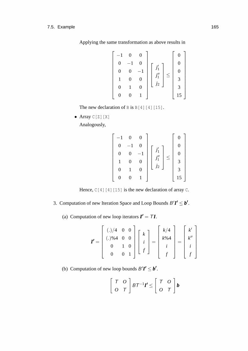
7.5. Example 165
Applying the same transformation as above results in
−1 0 0
0 −1 0
0 0 −1
1 0 0
0 1 0
0 0 1
j′1j′′1j2
≤
0
0
0
3
3
15
The new declaration of B is B[4][4][15].
• Array C[Z][X]
Analogously,
−1 0 0
0 −1 0
0 0 −1
1 0 0
0 1 0
0 0 1
j′1j′′1j2
≤
0
0
0
3
3
15
Hence, C[4][4][15] is the new declaration of array C.
3. Computation of new Iteration Space and Loop Bounds B ′III′′′ ≤ bbb′′′.
(a) Computation of new loop iterators III′′′ = T III.
III′′′ =
(.)/4 0 0
(.)%4 0 0
0 1 0
0 0 1
k
i
f
=
k/4
k%4
i
f
=
k′
k′′
i
f
(b) Computation of new loop bounds B ′III′′′ ≤ bbb′′′.
[
T O
O T
]
BT−1III′′′ ≤
[
T O
O T
]
bbb

166 Chapter 7. Parallelisation for Multi-DSP
Computing the left and right side of this inequality individually, this gives
B′ =
[
T O
O T
]
BT−1
=
[
T O
O T
]
−1 0 0
0 −1 0
0 0 −1
1 0 0
0 1 0
0 0 1
4 1 0 0
0 0 1 0
0 0 0 1
=
−1 0 0 0
0 −1 0 0
0 0 −1 0
0 0 0 −1
1 1 0 0
0 0 0 0
0 0 1 0
0 0 0 1
and similarly
bbb′′′ =
[
T O
O T
]
bbb
=
(.)/4 0 0 0 0 0
(.)%4 0 0 0 0 0
0 1 0 0 0 0
0 0 1 0 0 0
0 0 0 (.)/4 0 0
0 0 0 (.)%4 0 0
0 0 0 0 1 0
0 0 0 0 0 1
0
0
0
15
15
15
=
0
0
0
0
3
3
15
15

7.5. Example 167
i.e. the new loop bounds are
−1 0 0 0
0 −1 0 0
0 0 −1 0
0 0 0 −1
1 0 0 0
0 1 0 0
0 0 1 0
0 0 0 1
k′
k′′
i
f
≤
0
0
0
0
3
3
15
15
The upper loop bounds of the k′, k′′, i and f loops are 4, 4, 16 and 16,
respectively.
4. Update of array accesses U ′′III′′′+uuu.
U′′ = TUT−1
• Array access C[k][i]
U′′ =
(.)/4 0
(.)%4 0
0 1
[
1 0 0
0 1 0
]
4 1 0 0
0 0 1 0
0 0 0 1
=
1 0 0 0
0 1 0 0
0 0 1 0
i.e.
U′′III′′′+uuu =
1 0 0 0
0 1 0 0
0 0 1 0
k′
k′′
i
f
+
0
0
0
Hence, the access has the form C[k’][k’’][i].

168 Chapter 7. Parallelisation for Multi-DSP
• Array access A[i][f]
U′′III′′′+uuu =
0 0 (.)/4 0
0 0 (.)%4 0
0 0 0 1
k′
k“
i
f
+
0
0
0
Hence, the access has the form A[i/4)][i%4][f].
• Array access B[k][f]
U′′III′′′+uuu =
1 0 0 0
0 1 0 0
0 0 0 1
k′
k′′
i
f
+
0
0
0
Hence, the access has the form B[k’][k’’][f].
At this stage, the program shown in figure 7.12 is generated. Its data arrays are
partitioned and the outer loop is strip-mined. The next step is to parallelise this loop
across four processors, which is described in the following section.
7.5.4 Address Resolution
Figure 7.13 shows the matrix1 program (for processor 0 of a four processor machine)
after partitioning, mapping and address resolution. Following three relevant changes
have been made: (a) the outer (parallel) loop has been dropped and replaced by four
program copies with unique identifiers equal to the indices of the k1 loop, (b) the array
declarations have been replaced with distributed array declarations such that each of
the four programs and, therefore, each processor hosts only a single part of each array
locally, (c) descriptor data structures carrying the addresses as seen from a specific
processor have been introduced to all programs5.
5For the ease of presentation, certain type casts that are necessary to make the program in figure7.13 and in most subsequent examples fully ANSI-C compliant have been left out. A fully ANSI-Ccompliant versions of the program in figure 7.13 can be found in the appendix.
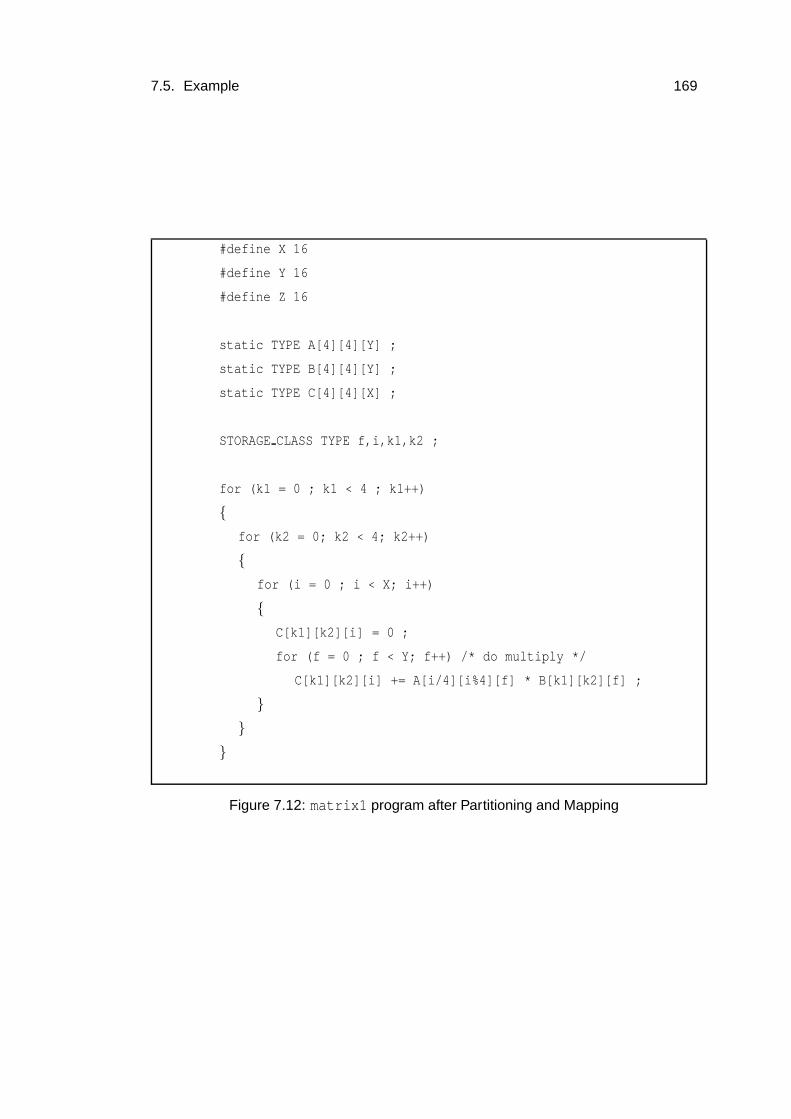
7.5. Example 169
#define X 16
#define Y 16
#define Z 16
static TYPE A[4][4][Y] ;
static TYPE B[4][4][Y] ;
static TYPE C[4][4][X] ;
STORAGE CLASS TYPE f,i,k1,k2 ;
for (k1 = 0 ; k1 < 4 ; k1++)
{
for (k2 = 0; k2 < 4; k2++)
{
for (i = 0 ; i < X; i++)
{
C[k1][k2][i] = 0 ;
for (f = 0 ; f < Y; f++) /* do multiply */
C[k1][k2][i] += A[i/4][i%4][f] * B[k1][k2][f] ;
}
}
}
Figure 7.12: matrix1 program after Partitioning and Mapping

170 Chapter 7. Parallelisation for Multi-DSP
The original declarations of the arrays A,B and C have been replace by more com-
plex declarations. Each array is split into four parts according to the previous par-
titioning and mapping stage. One part is declared to reside locally on processor 0.
The remaining parts of the arrays are declared extern, i.e. they are included into the
namespace of the program for processor 0, yet without allocating space for them. Fur-
thermore, an array of pointers is created for each distributed array. This array contains
as many entries as there are processors, i.e. four entries in this example. Unlike the
distributed arrays which reside on different processors without data replication, the de-
scriptor data structure is replicated on each processor and initialised with the addresses
of the partial data arrays. Any subsequent access to such a distributed array involves
two steps. E.g. the access C[k1][k2][i] first selects the k1-th element of the local
C data descriptor to determine the address (i.e. processor ID and local address) of the
relevant partial array, before the actual element is either locally or remotely accessed.
Each appearance of the index k1 is replaced by the unique ID MYID of the pro-
gram/processor. MYID represents exactly one value of the original k1 loop. Thus, each
instantiation of the program corresponds to one iteration of the dropped k1 loop. The
explicit k1 loop in figure 7.12 has been implicitly unrolled and distributed over four
program copies that run on different processors. Hence, the first index of each array
access does not only uniquely specify a particular iteration of the former k1 loop, but
also the location of the data.
7.5.5 Modulo Removal
In a final step, expensive modulo index expressions in the reference to array A are
eliminated. By strip-mining the i loop without applying any data transformation, the
mod and div expression disappear from the array reference and are replaced by more
“compiler-friendly” affine index expressions.
By construction, the transformation T which introduces mod and div index expres-
sions is known. Applying T to the enclosing loop iterators and updating the array
access matrices, however, recovers a modulo-free form. This transformation is applied
to the program in figure 7.13 where it eliminates integer division and modulo in the
reference to array A.
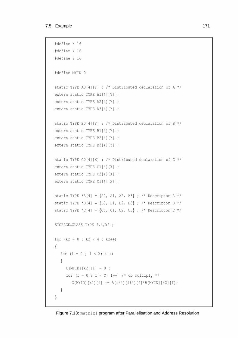
7.5. Example 171
#define X 16
#define Y 16
#define Z 16
#define MYID 0
static TYPE A0[4][Y] ; /* Distributed declaration of A */
extern static TYPE A1[4][Y] ;
extern static TYPE A2[4][Y] ;
extern static TYPE A3[4][Y] ;
static TYPE B0[4][Y] ; /* Distributed declaration of B */
extern static TYPE B1[4][Y] ;
extern static TYPE B2[4][Y] ;
extern static TYPE B3[4][Y] ;
static TYPE C0[4][X] ; /* Distributed declaration of C */
extern static TYPE C1[4][X] ;
extern static TYPE C2[4][X] ;
extern static TYPE C3[4][X] ;
static TYPE *A[4] = {A0, A1, A2, A3} ; /* Descriptor A */
static TYPE *B[4] = {B0, B1, B2, B3} ; /* Descriptor B */
static TYPE *C[4] = {C0, C1, C2, C3} ; /* Descriptor C */
STORAGE CLASS TYPE f,i,k2 ;
for (k2 = 0 ; k2 < 4 ; k2++)
{
for (i = 0 ; i < X; i++)
{
C[MYID][k2][i] = 0 ;
for (f = 0 ; f < Y; f++) /* do multiply */
C[MYID][k2][i] += A[i/4][i%4][f]*B[MYID][k2][f];
}
}
Figure 7.13: matrix1 program after Parallelisation and Address Resolution

172 Chapter 7. Parallelisation for Multi-DSP
The resulting program after modulo removal is shown in figure 7.14. The i has
been split into two new loops i1 and i2, and references to A, B and C have been updated
accordingly.
#define MYID 0
/* Array Declarations dropped */
STORAGE CLASS TYPE f,i1,i2,k2 ;
for (k2 = 0 ; k2 < 4 ; k2++)
{
for (i1 = 0 ; i1 < 4; i1++)
{
for (i2 = 0; i2 < 4; i2++)
{
C[MYID][k2][4*i1+i2] = 0 ;
for (f = 0 ; f < Y; f++) /* do multiply */
C[MYID][k2][4*i1+i2] += A[i1][i2][f] * B[MYID][k2][f];
}
}
}
Figure 7.14: matrix1 program after Modulo Removal
7.6 Related Work
Although a tremendous amount of work in automatic parallelisation can be found in the
world of High-Performance Computing, there is little work on parallelising compilers
for Multi-DSP.
A good overview of existing parallelisation techniques is given by Gupta et al.
(1999). Cache-coherent multiprocessors with distributed shared memory are the sub-

7.7. Conclusion 173
ject of Chandra et al. (1997). Although compilers for such machines must incorporate
data distribution and data locality increasing techniques (Carr et al., 1994; Tseng et al.,
1995), they are not faced with the problem of multiple, but globally-addressable ad-
dress spaces. Compiler-Implemented Shared Memory (CISM) as described by Larus
(1993) and Hiranandani et al. (1992) is a method to establish shared memory on
message-passing computers. However, these approaches assume separate distributed
address spaces and require complex run-time bookkeeping. Paraguin (Ferner, 2003) is
a compiler that generates message-passing code, but this compiler is still in its infancy
and requires user directives to drive its parallelisation.
An early paper (Teich and Thiele, 1991) described how DSP programs may be par-
allelised but gave no details or experimental results. Similarly, in Kalavade et al. (1999)
an interesting overall parallelisation framework is described but no mechanism or de-
tails of how parallelisation might take place is provided. In Lorts (2000) the impact of
different parallelisation techniques is considered, however, this was user-directed and
no automatic approach provided. In Karkowski and Corporaal (1998) a semi-automatic
parallelisation method to enable design-space exploration of different multi-processor
configurations based on the MOVE architecture is presented. However, no integrated
data partitioning strategy was available and data keeping is centralised. Furthermore,
in the experiments, communication was modelled in their simulator and thus the issue
of mapping parallelism combined with distributed address spaces was not addressed.
7.7 Conclusion
In this chapter a new compiler parallelisation approach that maps C programs onto
multiple address space multi-DSPs has been developed. Existing approaches to paral-
lelisation are not well suited for architectures with multiple visible address spaces. By
using a novel data transformation and an address resolution mechanism, single-address
space like parallel code can be generated for a multiple address space architecture with
resorting to message passing. The generated code is easy to read and amenable to
further sequential optimisation.

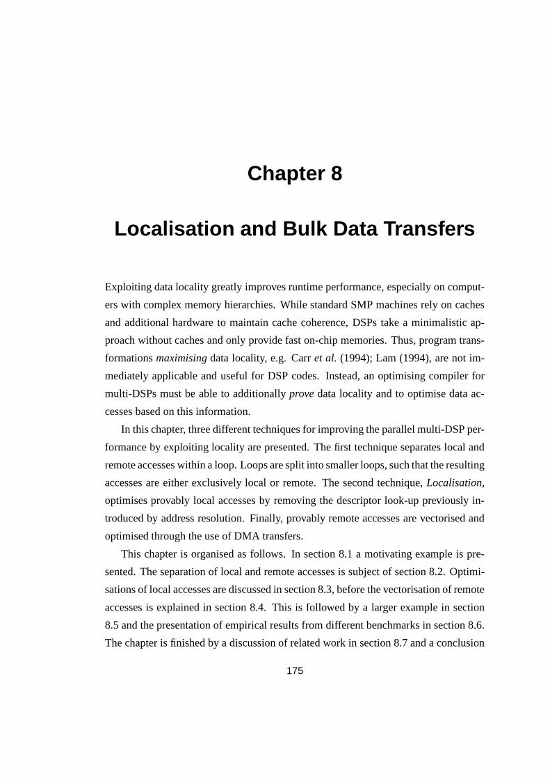
Chapter 8
Localisation and Bulk Data Transfers
Exploiting data locality greatly improves runtime performance, especially on comput-
ers with complex memory hierarchies. While standard SMP machines rely on caches
and additional hardware to maintain cache coherence, DSPs take a minimalistic ap-
proach without caches and only provide fast on-chip memories. Thus, program trans-
formations maximising data locality, e.g. Carr et al. (1994); Lam (1994), are not im-
mediately applicable and useful for DSP codes. Instead, an optimising compiler for
multi-DSPs must be able to additionally prove data locality and to optimise data ac-
cesses based on this information.
In this chapter, three different techniques for improving the parallel multi-DSP per-
formance by exploiting locality are presented. The first technique separates local and
remote accesses within a loop. Loops are split into smaller loops, such that the resulting
accesses are either exclusively local or remote. The second technique, Localisation,
optimises provably local accesses by removing the descriptor look-up previously in-
troduced by address resolution. Finally, provably remote accesses are vectorised and
optimised through the use of DMA transfers.
This chapter is organised as follows. In section 8.1 a motivating example is pre-
sented. The separation of local and remote accesses is subject of section 8.2. Optimi-
sations of local accesses are discussed in section 8.3, before the vectorisation of remote
accesses is explained in section 8.4. This is followed by a larger example in section
8.5 and the presentation of empirical results from different benchmarks in section 8.6.
The chapter is finished by a discussion of related work in section 8.7 and a conclusion
175

176 Chapter 8. Localisation and Bulk Data Transfers
in section 8.8.
8.1 Motivation
In the previously developed parallelisation scheme, descriptors to resolve accesses to
possibly remote arrays have been introduced. While these descriptors guarantee cor-
rectness of the parallel program, they introduce some indirection overhead for each
array access. Furthermore, the compiler cannot exploit lower latency and higher band-
width of local memory as each access can be potentially remote. Eliminating indirec-
tion for provably local accesses enables the compiler to identify local array access and
to optimise them accordingly. This is achieved during Localisation.
A second problem arises from the physically distributed organisation of memory in
multi-DSP. Unlike many other processors, DSPs usually do not contain (possibly co-
herent) caches, but contain fast software-managed on-chip memories, and, if required,
slower but larger off-chip memory. Data transfers between different memories and
processors can be sped up through the use Direct-Memory Access (DMA) engines that
operate autonomously and in parallel to the CPU core, once a transfer has been set
up. Under this scheme, transfers of infrequent, but large messages are favoured over
frequent, but small messages. To convert individual accesses to remote data into bulk
data transfers is the goal of Access Vectorisation (Li and Chen, 1991).
Naive SMP parallelisation is not sufficient to achieve any speedup over the sequen-
tial program. In particular, the additional overhead and excessive communication slow
down the matrix1 program to about 10% of its sequential performance (second bar in
figure 8.1). Partitioning and address resolution further penalise parallel performance
due to the increased number of memory accesses (third bar in figure 8.1). Combin-
ing partitioning, address resolution, localisation and access vectorisation, however,
improves performance dramatically. In fact, a linear performance increase on four
processors can be observed for this particular program (rightmost bar in figure 8.1).
The concepts presented in this chapter are illustrated in an example, before a the-
oretical framework is developed in the following sections. Figure 8.2 contains a small
program after parallelisation and address resolution. While this program has been cor-

8.1. Motivation 177
Figure 8.1: Impact of parallelisation, partitioning & address resolution and localisation
rectly parallelised, its performance is generally poor (see figure 8.1). The reason for
this lies in the backend compiler’s inability to distinguish between local and remote
accesses to arrays a, b and c. Further support is required to make local and remote
accesses explicit. Index set splitting can isolate local and remote accesses to c in sep-
arate loops, which are then amendable to further optimisation. Figure 8.3 shows the
effects of this transformations. The j1 loop effectively determines the location of the
access to c and has been split into three individual loops with ranges: 0 . . .(MYID−1),
MY ID, and (MYID+1) . . .4.
The array reference c[j1][j2] in the second loop of figure 8.3 is provably local,
since the only value j1 can take on is MYID. Therefore, the indirection step via the
data descriptor can be dropped and replaced by an immediate access to c0 (as MYID
= 0). This change is shown in figure 8.4. The locality of the access to c0 has been
made explicit for the backend compiler, which can, for example, generate accesses
considering higher bandwidth to and shorter latencies of local memory. In the first and
third loop, c[j1][j2] always references remote data since j1 never takes on the value
MYID. Hence, this remote access can be optimised based on this “remoteness” guar-

178 Chapter 8. Localisation and Bulk Data Transfers
#define MYID 0
int a0[8];
extern int a1[8],a2[8],a3[8];
int b0[8];
extern int b1[8],b2[8],b3[8];
int c0[8];
extern int c1[8],c2[8],c3[8];
int *a[4] = {a0,a1,a2,a2};
int *b[4] = {b0,b1,b2,b2};
int *c[4] = {c0,c1,c2,c2};
for(i = 0; i < 32; i++)
for(j1 = 0; j1 < 4; j1++)
for(j2 = 0; j2 < 8; j2++)
a[MYID][i] += b[MYID][i] * c[j1][j2];
Figure 8.2: Example program after parallelisation and address resolution (MYID = 0)

8.1. Motivation 179
#define MYID 0
/* Array Declarations dropped */
for(i = 0; i < 7; i++) {
/* a0, b0 local */
/* c remote */
for(j1 = 0; j1 < MYID; j1++)
for(j2 = 0; j2 < 8; j2++)
a[MYID][i] += b[MYID][i] * c[j1][j2];
/* a0, b0, c0 local */
for(j1 = MYID; j1 < MYID+1; j1++)
for(j2 = 0; j2 < 8; j2++)
a[MYID][i] += b[MYID][i] * c[j1][j2];
/* a0, b0 local */
/* c remote */
for(j1 = MYID+1; j1 < 4; j1++)
for(j2 = 0; j2 < 8; j2++)
a[MYID][i] += b[MYID][i] * c[j1][j2];
}
Figure 8.3: Example program after separation of local and remote accesses

180 Chapter 8. Localisation and Bulk Data Transfers
antee. The individual accesses to remote elements of c can be bundled or vectorised.
The difference to vectorisation in the message-passing world (Palermo et al., 1994) is,
however, that the presented method does not rely on message passing but perform a
simpler one-sided remote fetch operation (Message Passing Interface Forum, 1997).
#define MYID 0
/* Array Declarations dropped */
for(i = 0; i < 7; i++) {
/* a0, b0 local */
/* c remote */
for(j1 = 0; j1 < MYID; j1++)
for(j2 = 0; j2 < 8; j2++)
a0[i] += b0[i] * c[j1][j2];
/* a0, b0, c0 local */
for(j1 = MYID; j1 < MYID+1; j1++)
for(j2 = 0; j2 < 8; j2++)
a0[i] += b0[i] * c0[j2];
/* a0, b0 local */
/* c remote */
for(j1 = MYID+1; j1 < 4; j1++)
for(j2 = 0; j2 < 8; j2++)
a0[i] += b0[i] * c[j1][j2];
}
Figure 8.4: Example program after optimisation of local accesses
After index set splitting and localisation, only the first and the third of the j1 loops
contain remote accesses to array c. In the next step, these remote accesses are hoisted
and placed in separate Load Loops. Data is kept in local temporary buffers, which
are used in the Computational Loops instead. The effect of this transformation is

8.2. Access Separation 181
that the computational loops become entirely local, while the load loops can be further
optimised. Figure 8.5 contains the example program after the references to c[j1][j2]
have been isolated in separate load loops.
In the last transformation step, the individual accesses to remote data elements are
merged and replaced by calls to DMA routines. DMA transfers have the advantage
of requiring just a fixed, small number of bus transactions to request one large chunk
of remote data. Generally, the additional costs for setting up such a transfer amortise
already for small data block sizes. Consequently, many programs perform better (see
rightmost bar of figure 8.1) after this transformation due to a dramatic decrease of
communication latency. Figure 8.6 shows the example program after DMA transfers
have been inserted.
The final program as depicted in figure 8.6 is amendable to further transformations.
For example, the load loops can be hoisted out of the i loop at the cost of increased
memory requirements. Furthermore, despite the substantial modifications the program
is still amendable to the transformations evaluated in chapter 6.
8.2 Access Separation
Separation of local and remote accesses is the key factor to enable access optimisations
such as Localisation and DMA transfers. An approach to the Array Access Separation
Problem (AASP) that does not rely on expensive techniques such as Access Region
Analysis (Creusillet and Irigoin, 1995) is developed. Instead, it exploits properties of
the partitioning and mapping algorithm of chapter 7.3 to achieve the same result whilst
consuming fewer resources.
A brief overview of the standard approach to the AASP is given, before approach
exploiting explicit processor IDs is described.
8.2.1 Standard Approach
The standard approach to solving the AASP is to determine the range of loop index
values that produce references to local arrays. To achieve this, sophisticated techniques
that can deal with complex shapes of arrays, loops and index functions have been

182 Chapter 8. Localisation and Bulk Data Transfers
#define MYID 0
/* Array Declarations dropped */
for(i = 0; i < 7; i++) {
/* Load Loop */
/* Copy remote data to local temp buffer */
for(j1 = 0; j1 < MYID; j1++)
for(j2 = 0; j2 < 8; j2++)
temp[j1][j2] = c[j1][j2];
/* Compute Loop */
/* Reference to temp, entirely local */
for(j1 = 0; j1 < MYID; j1++)
for(j2 = 0; j2 < 8; j2++)
a0[i] += b0[i] * temp[j1][j2];
/* Compute Loop */
for(j1 = MYID; j1 < MYID+1; j1++)
for(j2 = 0; j2 < 8; j2++)
a0[i] += b0[i] * c0[j2];
/* Load Loop */
/* Copy remote data to local temp buffer */
for(j1 = MYID+1; j1 < 4; j1++)
for(j2 = 0; j2 < 8; j2++)
temp[j1][j2] = c[j1][j2];
/* Compute Loop */
/* Reference to temp, entirely local */
for(j1 = MYID+1; j1 < 4; j1++)
for(j2 = 0; j2 < 8; j2++)
a0[i] += b0[i] * temp[j1][j2];
}
Figure 8.5: Example program after introduction of load loops

8.2. Access Separation 183
#define MYID 0
/* Array Declarations dropped */
/* Compute Loop */
/* Reference to temp */
for(i = 0; i < 7; i++) {
/* Load Loop */
for(j1 = 0; j1 < MYID; j1++)
DMAget(&(temp[8*j1]), &(c[j1][0]), 8);
for(j1 = 0; j1 < MYID; j1++)
for(j2 = 0; j2 < 8; j2++)
a0[i] += b0[i] * temp[8*j1+j2];
/* Compute Loop */
for(j1 = MYID; j1 < MYID+1; j1++)
for(j2 = 0; j2 < 8; j2++)
a0[i] += b0[i] * c0[j2];
/* Load Loop */
for(j1 = MYID+1; j1 < 4; j1++)
DMAget(&(temp[8*j1]), &(c[j1][0], 8);
/* Compute Loop */
/* Reference to temp */
for(j1 = MYID+1; j1 < 4; j1++)
for(j2 = 0; j2 < 8; j2++)
a0[i] += b0[i] * temp[8*j1+j2];
}
Figure 8.6: Example program with inserted DMA transfers

184 Chapter 8. Localisation and Bulk Data Transfers
developed (Creusillet and Irigoin, 1995; Hoeflinger et al., 1996). A simple technique
for affine array index function is shown below. Given this restriction, the formulation
of the AASP is relatively easy. Using the same notation as in chapter 7, affine array
references can be described by UIII + uuu, the global and local array index spaces by
AJJJ ≤ aaa and A′JJJ ≤ aaa′′′, respectively, and the loop bounds by BIII ≤ bbb.
Substitution of JJJ in A′JJJ ≤ aaa′′′ by JJJ = UIII +uuu and extending the resulting constraint
system by BIII≤ bbb results in a description of the new loop bounds for which the accesses
are local. Substituting
JJJ = UIII +uuu (8.1)
in
(A′JJJ ≤ aaa′′′) = (A′(UIII +uuu)≤ aaa′′′) = A′UIII +A
′uuu≤ aaa′′′ (8.2)
results in
A′UIII ≤ aaa′′′−A
′uuu (8.3)
Incorporating the original loop bound constraints results in
[
A′UB
]
III ≤
[
aaa′′′−Auuu
bbb
]
(8.4)
which is the restricted range of the loop B ′III ≤ bbb′′′ in which it produces local array
accesses.
This iteration space B ′III ≤ bbb′′′ can be split from the original iteration space and the
corresponding loop further optimised. The main problem, however, is to compute the
iteration space of the resulting remote loop, i.e.
(BIII ≤ bbb)− (B ′III ≤ bbb′′′) (8.5)
This computation requires the subtraction of two sets (Hoeflinger et al., 1996), an
operation which is often prohibitive due to its high complexity.
To accomplish the full separation of local and remote accesses, the computation
above must be repeated for each array and each remote location (i.e. each processor).
That is, for each processor x and for all processors z ∈ {1, . . . , p}\{x}
BxIII ≤ bbbx∩ (BzIII ≤ bbbz∧ JJJz = UIIIz +uuu) (8.6)

8.2. Access Separation 185
must be determined. This approach is clearly not feasible for anything more complex
than most trivial examples.
An alternative approach to access separation which exploits a property of the em-
ployed partitioning scheme to reduce its complexity is presented in the following sec-
tion.
8.2.2 Access Separation Based on Explicit Processor IDs
Array access separation is greatly simplified when the explicit processor ID introduced
by partitioning and mapping algorithm of chapter 7 is incorporated. To identify local
accesses only the location determining indices of a given array reference must be con-
sidered. The relevant indices are known at this stage as they have been previously used
to construct the partition matrix P . The points in the iteration space of the embrac-
ing loop nest where these location determining indices equal the processor ID produce
local accesses.
Any such array reference identified as mixed local and remote is taken as a basis
for the splitting of the iteration set of its embracing loop. Despite the fact that this
transformation splits the iteration set of a loop, it is usually referred to as Index Set
Splitting (Griebl et al., 2000). Three new loops are constructed, which together cover
the entire iteration space of the original loop. The first loop spans from the lower
bound of the original loop to just below the current processor ID, MYID. The second
loop contains a single iteration for MYID, and the last loop covers the iterations from
MYID+1 to the upper bound of the original loop. If partitioning has been performed
along several dimensions, index splitting must also be performed on each of them.
In general, this loop transformation can be described as follows. For each dimen-
sion partitioned, the index set of the corresponding loop is split into three adjacent
subranges (before split point, on split point, and after split point) each of which is
represented by a new loop on the same nesting level as the original loop. The second
subrange, however, only consists of a single point, i.e. a single iteration. Thus, the
loop for this single iteration can be collapsed and its loop body exposed.
Theorem 8.1 Partitioning a loop nest along d dimensions produces n = 2× d + 1
resulting loops.

186 Chapter 8. Localisation and Bulk Data Transfers
Proof 8.1 The induction hypothesis to proof theorem 8.1 is n = 2×d +1 for d dimen-
sions to partition along.
1. Base case (d = 1)
Index set splitting along a single dimension splits a single loop into three adja-
cent subranges, i.e. the total number of loops after index set splitting is three. It
is n = 2×1+1 = 3.
2. Induction step (d→ (d +1))
It is assumed that index set splitting has been applied to d dimensions and that
n = 2×d +1 loops have been created on the outermost nesting level. Further in-
dex set splitting of inner loops of the “prologue” and “epilogue” loops does not
expose new loops to the outermost nesting level, but only increases the number of
loops in their loop bodies. Only the single iteration “middle” loop is dismantled
and contributes to the creation of three new loops on the outermost nesting level
(see figure 8.7). It holds n = 2×d +1−1+3 = 2×d +3 = 2× (d +1)+1 for
the number of resulting loops. �
In the example in figure 8.7, splitting is performed first along the dimension of the
i-loop, and then along the j-loop. The single loop nest in figure 8.7(a) is converted into
three loops in figure 8.7(b), and repeated index set splitting produces five loop nests
(loops 1, 2.1, 2.2, 2.3, and 3) in figure 8.7(c).
Technically, index set splitting is performed by appropriately constraining the iter-
ation set BIII ≤ bbb of the loop to split by a set of constraints C0, C1 and C2. These three
constraints represent the cases < MY ID, = MY ID and > MY ID where MY ID is the
ID of the current processor. Formally, for each remote reference, the original loop is
partitioned into n separate loop nests using index set splitting:
Q(BIII ≤ bbb,Q1) 7→ Qi(BIII ≤ bbb∧Ci,Q1),∀i ∈ 0, . . . ,n−1 (8.7)
where n = 2d + 1 and d is the number of dimensions partitioned. This transforma-
tion (7→) maps a computation set Q with the iteration space BIII ≤ bbb and an enclosed
computation set Q1 onto a sequence of n appropriately constrained computation sets
Qi.

8.2. Access Separation 187
00: for(i = 0; i < 4; i++) {
01: for(j = 0; j < 4; j++) {
02: for(k = 0; k < 4; k++) {
03: ...
04: }
05: }
06: }
07:
08:
09:
10:
11:
12:
13:
14:
15:
16:
17:
18:
19:
20:
21:
22:
23:
24:
25:
26:
27:
28:
29:
30:
31:
32:
33:
34:
35:
36:
37:
38:
39:
40:
41:
42:
43:
44:
45:
46:
47:
48:
49:
50:
51:
52:
53:
54:
55:
56:
(a) Original loop nest
00: /* Loop 1 */
01: for(i = 0; i < MYID; i++) {
02: for(j = 0; j < 4; j++) {
03: for(k = 0; k < 4; k++) {
04: ...
05: }
06: }
07: }
08:
09: /* Loop 2 */
10: for(j = 0; j < 4; j++) {
11: for(k = 0; k < 4; k++) {
12: ...
13: }
14: }
15:
16: /* Loop 3 */
17: for(i = MYID+1; i < 4; i++) {
18: for(j = 0; j < 4; j++) {
19: for(k = 0; k < 4; k++) {
20: ...
21: }
22: }
23: }
24:
25:
26:
27:
28:
29:
30:
31:
32:
33:
34:
35:
36:
37:
38:
39:
40:
41:
42:
43:
44:
45:
46:
47:
48:
49:
50:
51:
52:
53:
54:
55:
56:
(b) Splitting the i-loop
00: /* Loop 1 */
01: for(i = 0; i < MYID; i++) {
02: /* Loop 1.1 */
03: for(j = 0; j < MYID; j++) {
04: for(k = 0; k < 4; k++) {
05: ...
06: }
07: /* Loop 1.2 */
08: for(k = 0; k < 4; k++) {
09: ...
10: }
11: /* Loop 1.3 */
12: for(j = MYID+1; j < 4; j++) {
13: for(k = 0; k < 4; k++) {
14: ...
15: }
16: }
17: }
18:
19: /* Loop 2.1 */
20: for(j = 0; j < MYID; j++) {
21: for(k = 0; k < 4; k++) {
22: ...
23: }
24: }
25:
26: /* Loop 2.2 */
27: for(k = 0; k < 4; k++) {
28: ...
29: }
30: }
31:
32: /* Loop 2.3 */
33: for(j = MYID+1; j < 4; j++) {
34: for(k = 0; k < 4; k++) {
35: ...
36: }
37: }
38:
39: /* Loop 3 */
40: for(i = MYID+1; i < 4; i++) {
41: /* Loop 3.1 */
42: for(j = 0; j < MYID; j++) {
43: for(k = 0; k < 4; k++) {
44: ...
45: }
46: /* Loop 3.2 */
47: for(k = 0; k < 4; k++) {
48: ...
49: }
50: /* Loop 3.3 */
51: for(j = MYID+1; j < 4; j++) {
52: for(k = 0; k < 4; k++) {
53: ...
54: }
55: }
56: }
(c) Splitting the i- and j-loops
Figure 8.7: Example illustrating index set splitting

188 Chapter 8. Localisation and Bulk Data Transfers
For the program in figure 8.2 partitioning is performed along one dimension, hence
n = 3. The constraints resulting from intersecting 0, . . . ,3 with < MY ID, = MY ID and
> MY ID, respectively, are
C0 : 0≤ j1 ≤ (MYID−1) (8.8)
C1 : j1 = MY ID (8.9)
C2 : (MY ID+1)≤ j1 ≤ 3 (8.10)
From this, the program in figure 8.3 is generated.
Exploiting explicit processor IDs as introduced by the parallelisation scheme de-
scribed in chapter 7 eliminates the need for expensive access region analyses to sepa-
rate local and remote array references.
8.3 Local Access Optimisations
After separating local and remote references, accesses to local arrays can bypass the
array descriptor data structure introduced as part of the address resolution mechanism.
One level of indirection for each array access can be eliminated, thus the number of
memory accesses is reduced significantly. In addition, references to local data are made
explicit such that the backend compiler is enabled to produce more efficient code.
Checking each array reference whether it accesses local data is simple, once local
and remote accesses have been separated. It is assumed that single iteration loops as
introduced by index set splitting have been collapsed and their constant index propa-
gated. A simple check whether the location determining indices of an array reference
are constant and equal to the processor ID, MYID, is sufficient to prove an array access
local. If this is the case, the lookup in the data descriptor can be dropped and, instead,
the local array partition is accessed directly.
This is a simple syntactic transformation. Given an array reference X [UIII +uuu], the
dimension δ ∈ 0, . . . ,N− 1 of partitioning and the syntactic concatenation operator :
it is
X [UIII +uuu] 7→ X : uδ[UδIII +uuuδ] (8.11)

8.4. Remote Access Vectorisation 189
where X is the name of a descriptor array, uδ the δ’th component of uuu, and UδIII +
uuuδ the index vector resulting from removing the δ’th component of the vector UIII +
uuu (projection). This transformation replaces an indirect array reference based on a
descriptor lookup with an immediate reference to the corresponding local array.
For example, in figure 8.3 the reference a[MYID][i] with constant MY ID, e.g.
MY ID = 0, is replaced by a0[i]. Applying this to all references with constant first
index in the example in figure 8.3 produces the code in figure 8.4, where all accesses
to a0, b0 and c0 can be statically identified as local by the backend compiler.
8.4 Remote Access Vectorisation
Repeated reference to a remote data item will incur multiple remote accesses. Bundling
remote references in a bulk DMA data transfer gives better performance due to amor-
tised transfer costs. In this section, the isolation and subsequent transformation of
remote array accesses is explained. Temporal and spatial locality is considered, and
DMA-based data transfers are automatically inserted.
8.4.1 Load Loops
Load loops are introduced to separate local from remote accesses. Remote references
are hoisted from the original loop and placed inside the load loop, where the remote
data is copied into a locally allocated temporary buffer. The Compute Loop refers to
that buffer instead and operates entirely on local data.
The transformation is of the form
Q 7→ (Q1, . . . ,QK) (8.12)
where K− 1 is the number of remotely accessed arrays in Q. A single loop nest Q
is distributed so that there are now K loop nests, K− 1 of which are load loops. In
example 8.4, there is only one remote array, hence K = 2.
In general, there exists more than one loop embracing a remote reference. Hence,
there are several options on how far to hoist the reference as to maximise performance.
Given that data dependences permit, hoisting to the outermost level surely increases

190 Chapter 8. Localisation and Bulk Data Transfers
performance most as the number of transfers is minimised. However, the required
temporary buffer space also increases and the restricted amount of available memory
might be prohibitive.
Possible solutions to this problem is discussed in the following paragraph in the
context of data buffer allocation.
8.4.1.1 Data buffer allocation
Before any remote access optimisation can take place, sufficient storage to hold tem-
porary data must be allocated. Two methods for the allocation data buffer storage are
presented. The first one is fast, but entirely static and does not necessarily utilise all
available memory. The second approach is more flexible, but of higher complexity
since it requires two compilation passes. In the first pass, the remaining memory avail-
able for buffers is determined, and in the second pass the loop nest is split at a level
such that most benefit can be taken from the available storage.
A simple method for the allocation of data buffers is to chose a fixed size s of
available storage, and check that the remote data fits, i.e.
‖Ul,...,nIIIl,...,n‖ ≤ s (8.13)
where Ul,...,n and IIIl,...,n are the projected access matrix U and the projected iteration
vector III for a particular nesting level l of a loop nest. Equation 8.13 determines the
range of accessed array elements at levels l, . . . ,n of a loop nest and from this the
absolute memory requirements are determined.
In figure 8.8 an algorithm is presented that determines the level of hoisting for a
given fixed buffer size s. Starting at the outermost possible, i.e. legal with respect
to data dependences, loop of a loop nest the condition in equation 8.13 is repeatedly
checked until a level is reached where the available buffer is large enough to keep the
remote data. Further hoisting the load operation results in smaller number of expensive
remote accesses, but may increase the size of the temporary data buffer. Inspecting
loop nests from the outermost to the innermost level minimises the number of remote
accesses, whilst meeting the given buffer size constraint.
As this approach is not very flexible, another dynamic approach is proposed and
presented in figure 8.9. After compiling and linking the program without reserving

8.4. Remote Access Vectorisation 191
1. Parameters
Given: loop nest Q with depth n, access matrix U, buffer size constraint s.
2. Determine level of hoisting
(a) Level l = 1;
(b) While (‖Ul,...,nIIIl,...,n‖> s) And (l ≤ n) Do
l = l +1;
3. Code generation
(a) Insert load loops at level l.
(b) Allocate buffer of size s.
Figure 8.8: Static algorithm to determine level of hoisting
any data buffers, the total amount of memory used by the program can be determined
from the linker log files. Comparing this value to the known total memory of the target
processor gives the available size storage s available for buffering. With this value,
a buffer of maximal size can be allocated without exceeding the processor’s on-chip
memory limit. This value also determines the splitting level the loop nest as in the first
approach.
8.4.2 Access Vectorisation
Up to this point, remote accesses have been isolated and moved into separate Load
Loops. The following transformation sequence substitutes these loops with explicit
calls to DMA functions, which automate the transfer of larger data blocks.
First, temporal locality in the load loops is exploited such that redundant loops
can be dropped. Then, accesses to remote data must be transformed into unit stride
order allowing DMA engines to access the data sequentially. As local data buffers
are organised as linear arrays, but accesses in the compute loops might assume multi-
dimensional arrays, these accesses must be linearised to match the actual linear buffer

192 Chapter 8. Localisation and Bulk Data Transfers
1. Code generation
Generate program without load loops and temporary data buffers.
2. Compile and link
Compile program, generate memory usage log.
3. Determine buffer size
Determine remaining memory space in data memory segment.
4. Allocate buffer
Determine level of hoisting, generate load loops and allocate temporary buffer as in
algorithm 8.8.
Figure 8.9: Dynamic data buffer allocation algorithm
organisation. Finally, strip-mining the load loops and replacing the assignment state-
ments of the innermost loop with DMA functions convert the loop into its final form.
8.4.2.1 Locality Optimisation
Temporal locality in the load loops corresponds to an invariant access iterator or the
null space of the access matrix, i.e. N (U). There always exists a transformation T ,
found by reducing U to Smith-Normal form (Ayres, 1962) that transforms the iteration
space such that the invariant iterator(s) is innermost and can be removed by Fourier-
Motzkin elimination (Schrijver, 1986). There are no invariant iterators in the load
loops of figure 8.5.
8.4.2.2 Unit-Stride Transformation
To copy a block of remote data in a single transfer, it must be accessed in unit stride
order. This can be created by a simple loop transformation T , T = U.
In example 8.5, T is the identity transformation as the accesses in the load loop is
already in stride-1 order.

8.4. Remote Access Vectorisation 193
8.4.2.3 Access Linearisation
All remote data is finally copied into the same linear temporary buffer. The original
remote arrays, however, might be of higher dimension. If this linear buffer organisation
is not yet present, the temporary array and all the accesses to it must be linearised
throughout the program. This is done with following data transformation
U′t = LUt (8.14)
In the example, L =[
8 1]
. Array accesses are transformed from temp[j1][j2]
to temp[8*j1+j2] in figure 8.6.
8.4.2.4 DMA Transfers
A DMA transfer requires the addresses of the remote data and the local buffer, and the
amount of data to be transferred. Insertion of a DMA call effectively vectorises the
load loop and replaces the innermost loop. The start address of the remote data can be
computed using the array base address and the lower loop bound. The vector stride is
equal to the loop range. Thus, the remote array reference is transformed as follows
UM = 0,uM = min(Im) (8.15)
where the M’th row corresponding to the innermost index is deleted in the array ac-
cess matrix U and min(Im) denotes the lower loop bound of the innermost loop. The
reference to the temporary array is similarly updated, and Im is eliminated by Fourier-
Motzkin elimination. Also non-constant lower loop bounds are subject to Fourier-
Motzkin elimination. Constant non-zero offsets to the temporary buffer are adjusted
by shifting of the corresponding elements of the constant offset vector uuu and propagat-
ing this index shift to the sites of its use. Finally, the assignment statement is replaced
by a generic DMA transfer call DMAget(&tempref, &remoteref, size) to the pro-
duce the final code.
For example, the j2 loop in the first load loop in figure 8.5 is vectorised by the
insertion of a DMA call. As a consequence, the loop is dropped and the reference
c[j1][j2] is converted to c[j][0] as shown in figure 8.6. The vector stride in this
example is eight as this is the loop range of the eliminated j2 loop.

194 Chapter 8. Localisation and Bulk Data Transfers
8.5 Example
In this section, the matrix multiplication kernel matrix1 is again used to demonstrate
the transformation developed in this chapter.
The initial parallel matrix1 program after partitioning, mapping, address resolu-
tion and parallelisation is shown in figure 8.10. In this program, accesses to array A are
not constantly local or remote, because of their dependence on the loop iterator i1 in
the first position of the reference A[i1][i2][f]. Index set splitting is applied on the
i1 loop to separate local and remote accesses to A.
#define MYID 0
/* Array Declarations dropped */
STORAGE CLASS TYPE f,i1,i2,k2 ;
for (k2 = 0 ; k2 < 4 ; k2++)
{
for (i1 = 0 ; i1 < 4; i1++)
{
for (i2 = 0; i2 < 4; i2++)
{
C[MYID][k2][4*i1+i2] = 0 ;
for (f = 0 ; f < 16; f++) /* do multiply */
{
C[MYID][k2][4*i1+i2] += A[i1][i2][f] * B[MYID][k2][f];
}
}
}
}
Figure 8.10: Initial parallel matrix1 program
Figure 8.11 shows the program after the i1 loop has been split into three separate

8.5. Example 195
loops, of which the second one contains only one iteration and is entirely local. As
there is only one iteration, the loop header of this second loop can be dropped, and all
occurrences of i1 in the loop body can be substituted by MYID. Identifying the local
array accesses is straightforward, since this amounts to searching for array references
with a constant first index equal to the current processor ID (MYID). Descriptor lookups
for local accesses are dropped, because local data arrays can always be accessed di-
rectly. The result of this localisation optimisation is also shown in figure 8.11. Since
MYID = 0 is assumed in this example, references to A[MYID], B[MYID] and C[MYID]
are converted to A0, B0 and C0, respectively.
The second loop of the program in figure 8.11 and the accesses to B and C in the
other loops are now entirely local. Only the first and third loop contain remote refer-
ences to A. As the array A is referenced element-wise, many cycles are wasted in bus
transactions. Vectorising remote accesses greatly improves efficiency. In a first step,
the accesses to the array A are hoisted from the relevant loops and placed in Load Loop.
Remote data is copied to a local temporary buffer, which is then used in the Compute
Loop. In the example in figure 8.11, there are four different options as to where to
place the load loop:
1. In front of the f loop, or
2. in front of the i2 loop, or
3. in front of the i1 loop, or
4. in front of the k2 loop.
Each of the possible options has its specific advantages and disadvantages as sum-
marised in figure 8.12.
Hoisting the accesses to A out of the outermost loop k2 clearly minimises the num-
ber of transactions, but might easily exceed the memory resources since the entire A
matrix must fit onto each processor in addition to the partitions of B and C. Obviously,
the savings on memory resources from placing the load loop in front of the i1 loop
are minimal over placement in front of the k2 loop. The number of bus transactions
is increased significantly, while the memory requirements on individual processors are
196 Chapter 8. Localisation and Bulk Data Transfers
#define MYID 0
/* Array Declarations dropped */
STORAGE CLASS TYPE f,i1,i2,k2 ;
for (k2 = 0 ; k2 < 4 ; k2++) {
for (i1 = 0 ; i1 < MYID; i1++) {
for (i2 = 0; i2 < 4; i2++) {
C0[k2][4*i1+i2] = 0 ;
for (f = 0 ; f < 16; f++) /* do multiply */
C0[k2][4*i1+i2] += A[i1][i2][f] * B0[k2][f];
}
}
/* i1 loop dropped */
for (i2 = 0; i2 < 4; i2++) {
C0[k2][4*MYID+i2] = 0 ;
for (f = 0 ; f < 16; f++) /* do multiply */
C0[k2][4*MYID+i2] += A0[i2][f] * B0[k2][f];
}
for (i1 = MYID+1 ; i1 < 4; i1++) {
for (i2 = 0; i2 < 4; i2++) {
C0[k2][4*i1+i2] = 0 ;
for (f = 0 ; f < 16; f++) /* do multiply */
C0[k2][4*i1+i2] += A[i1][i2][f] * B0[k2][f];
}
}
}
Figure 8.11: matrix1 program after separation of local/remote accesses and optimisa-
tion of local array accesses

8.5. Example 197
Option # of transactions Local buffer size Comments
(in front of)
f 3× Z4 ×
X4 Y One remote row of A buffered locally
i2 3× Z4
X4 ×Y One remote block of A buffered locally
i1 3× Z4 up to 3× X
4 ×Y A completely stored locally on some processors
k2 3 3× X4 ×Y A completely stored locally on all processors
(original) 3× Z4 ×
X4 ×Y 1 One remote element of A fetched at a time
Figure 8.12: Memory requirements and total number of communications for different
Load Loop placements in the matrix1 example
not reduced. Placing the load loops in front of the i2 and f loops, respectively, further
increases the number of transactions, but reduces the storage requirements to the local
temporary buffer.
For the subsequent transformations it is assumed that up to X4 ×Y elements can
be buffered locally without exceeding any processor’s on-chip memory limit. Thus,
remote accesses can be safely hoisted out the f and i2 loops, but not further.
In the program in figure 8.13 remote accesses have been isolated in load loop,
but are still performed element-wise. In the next step, the two innermost loops are vec-
torised and replaced by a call to a DMA transfer routine. The effect of this replacement
is that only one transfer per remote processor is performed within the i1 loop rather
than one transfer per remote data element. This dramatically reduces the communi-
cation time, and, therefore, improves the overall performance. Figure 8.14 shows the
corresponding code excerpt. Furthermore, all accesses to the temporary buffer temp
have been linearised for more flexible use.
Neither the k loop nor the i2 loop of the example in figure 8.13 cause a temporal
reuse of elements of the array A. Therefore, no further transformation is necessary at
this stage. However, if the load operations had been hoisted out of the k2 loop instead,
it would have been necessary to eliminate that outer loop from the generated load loop.
At this stage, the generated program is optimised to exploit local and remote ac-
cess efficiently. Local buffers and DMA calls have been inserted to make use of higher
bandwidth to local memory and available DMA controllers, while hard memory con-
straints are still met. In chapter 9.2.1 further communication optimisations, e.g. over-

198 Chapter 8. Localisation and Bulk Data Transfers
for (k2 = 0 ; k2 < 4 ; k2++) {
for (i1 = 0 ; i1 < MYID; i1++) {
/* Load Loop */
for (i2 = 0; i2 < 4; i2++)
for (f = 0 ; f < 16; f++)
temp[i2][f] = A[i1][i2][f];
/* Compute Loop */
for (i2 = 0; i2 < 4; i2++) {
C0[k2][4*i1+i2] = 0 ;
for (f = 0 ; f < 16; f++) /* do multiply */
C0[k2][4*i1+i2] += temp[i2][f] * B0[k2][f];
}
}
/* i1 loop dropped */
/* Local Compute Loop */
for (i2 = 0; i2 < 4; i2++) {
C0[k2][4*MYID+i2] = 0 ;
for (f = 0 ; f < 16; f++) /* do multiply */
C0[k2][4*MYID+i2] += A0[i2][f] * B0[k2][f];
}
for (i1 = MYID+1 ; i1 < 4; i1++) {
/* Load Loop */
for (i2 = 0; i2 < 4; i2++)
for (f = 0 ; f < 16; f++)
temp[i2][f] = A[i1][i2][f];
/* Compute Loop */
for (i2 = 0; i2 < 4; i2++) {
C0[k2][4*i1+i2] = 0 ;
for (f = 0 ; f < 16; f++) /* do multiply */
C0[k2][4*i1+i2] += temp[i2][f] * B0[k2][f];
}
}
}
Figure 8.13: matrix1 program after introduction of load loops

8.5. Example 199
for (k2 = 0 ; k2 < 4 ; k2++) {
for (i1 = 0 ; i1 < MYID; i1++) {
/* Load Loop */
DMAget(&(temp[0]),&(A[i1][0][0]),4*16);
/* Compute Loop */
for (i2 = 0; i2 < 4; i2++) {
C0[k2][4*i1+i2] = 0 ;
for (f = 0 ; f < 16; f++) /* do multiply */
C0[k2][4*i1+i2] += temp[4*i2+f] * B0[k2][f];
}
}
/* Local Compute Loop */
for (i2 = 0; i2 < 4; i2++) {
C0[k2][4*MYID+i2] = 0 ;
for (f = 0 ; f < 16; f++) /* do multiply */
C0[k2][4*MYID+i2] += A0[i2][f] * B0[k2][f];
}
for (i1 = MYID+1 ; i1 < 4; i1++) {
/* Load Loop */
DMAget(&(temp[0]),&(A[i1][0][0]),4*16);
/* Compute Loop */
for (i2 = 0; i2 < 4; i2++) {
C0[k2][4*i1+i2] = 0 ;
for (f = 0 ; f < 16; f++) /* do multiply */
C0[k2][4*i1+i2] += temp[4*i2+f] * B0[k2][f];
}
}
}
Figure 8.14: matrix1 program after temporary buffer access linearisation and DMA
transfer insertion

200 Chapter 8. Localisation and Bulk Data Transfers
lapping communication and computation, are outlined.
8.6 Empirical Results
The effectiveness of the parallelisation scheme is evaluated against two different bench-
mark sets: DSPstone1 (Zivojnovic et al., 1994) and UTDSP (Lee, 1998). The programs
were executed on a Transtech TS-P36N board with a cluster of four cross-connected
250MHz TigerSHARC TS-101 DSPs, and all additionally sharing the same external
bus and 128MB of external SDRAM. The programs were compiled with the Analog
Devices VisualDSP++ 2.0 Compiler (version 6.1.18) with full optimisation; all timings
are cycle accurate.
8.6.1 Parallelism Detection
Figure 8.17 shows the set of loop-based DSPstone programs. Initially, the compiler
fails to parallelise these programs because they make an extensive use of pointer arith-
metic for array traversals, as shown in the second column. However, after applying
array recovery (column 3) most of the programs become parallelisable (column 4). In
fact, the only program that cannot be parallelised after array conversion (biquad) con-
tains a cross-iteration data dependence that does not permit parallelisation. adpcm is
the only program in this benchmark set that cannot be recovered due to its complex-
ity. The fifth column of figure 8.17 shows whether or not a program can be profitably
parallelised. Programs comprising of only very small loops such as dot product and
matrix1x3 perform better when executed sequentially due to the overhead associated
with parallel execution and are filtered out, at stage 2, by the parallelisation algorithm.
As far as UTDSP is concerned, many of the programs are available in their original
pointer-based form as well as in an array-based form. Wherever possible, the array-
based programs are taken as a starting point for parallelisation2. The impact of modulo
removal can be seen in figure 8.18. Four of the UTDSP programs (iir, adpcm, fir and
1Artificially small data set sizes have been selected by its designers to focus on code generation; ascaled version is used wherever appropriate.
2Array recovery on the pointer programs gives an equivalent array form

8.6. Empirical Results 201
Figure 8.15: Total Speedup for DSPstone benchmarks
lmsfir) can be converted into a modulo-free form through program recovery. Modulo
removal has a direct impact on the paralleliser’s ability to successfully parallelise those
programs – three out of four programs could be parallelised after the application of
this transformation. ADPCM cannot be parallelised after modulo removal due to data
dependences.
Although program recovery is used largely to facilitate parallelisation and multi-
processor performance, it can impact sequential performance as well. The first two
columns of each set of bars in figures 8.15 and 8.16 show the original sequential time
and the speedup after program recovery. Three out of the eight DSPstone benchmarks
benefit from this transformation, whereas only a single kernel (fir) experiences a per-
formance degradation after program recovery. In fir2dim,lms and matrix2, array

202 Chapter 8. Localisation and Bulk Data Transfers
Figure 8.16: Total Speedup for UTDSP benchmarks
recovery has enabled better data dependence analysis and allowed a tighter scheduling
in each case. fir has a very small number of operations such that the slight over-
head of enumerating array subscripts has a disproportional effect on its performance.
Figure 8.16 shows the impact of modulo removal on the performance of the UTDSP
benchmark. Since a computation of a modulo is a comparatively expensive operation,
its removal positively influences the performance of the three programs wherever it is
applicable.
8.6.2 Partitioning and Address Resolution
The third column of each set of bars in figures 8.15 and 8.16 shows the effect of blindly
using a single-address space approach to parallelisation without data distribution on a
multiple-address space machine. Not surprisingly, performance is universally poor.

8.6. Empirical Results 203
Figure 8.17: Exploitable Parallelism in DSPstone
The fourth column in each figure shows the performance after applying data partition-
ing, mapping and address resolution. Although some programs experience a speedup
over their sequential version (convolution and fir2dim), the overall performance is
still disappointing. After a closer inspection of the generated assembly codes, it ap-
pears that the Analog Devices compiler cannot distinguish between local and remote
data. It conservatively assumes all data is remote and generates “slow” accesses, dou-
ble word instead of quad word, to local data. An increased memory access latency
is accounted for in the produced VLIW schedule. In addition, all remote memory
transactions occur element-wise and do not effectively utilise the DMA engine.
8.6.3 Localisation
The final columns of figures 8.15 and 8.16 show the performance after the locality
optimisations are applied to the partitioned code. Accesses to local data are made ex-
plicit, so the compiler can identify local data and is able to generate tighter and more
efficient schedules. In addition, remote memory accesses are grouped to utilise the
DMA engine. In the case of DSPstone, linear or superlinear speedups are achieved for
all programs bar one (fir), where the number of operations is very small. Superlinear
speedup occurs in precisely those cases where program recovery has given a sequen-

204 Chapter 8. Localisation and Bulk Data Transfers
Figure 8.18: Exploitable Parallelism in UTDSP
tial improvement over the pointer based code. The overall speedups vary between 1.9
(fir) and 6.5 (matrix2), their average is 4.28 on four processors. The overall speedup
for the UTDSP benchmarks is less dramatic, as the programs are more complex, in-
cluding full applications, and have a greater communication overhead. These programs
show speedups between 1.33 and 5.69, and an average speedup of 3.65. LMSFIR and
Histogram fail to give significant speedup due to the lack of sufficient data paral-
lelism inherent in the programs. Conversely, FIR, MULT(large), Compress and JPEG
Filter give superlinear speedup due to improved sequential performance of the pro-
grams after parallelisation. As the loops are shorter after parallelisation, it appears that
the native loop unrolling algorithm performs better on the reduced trip count.
8.7 Related Work
There is an extremely large body of work on compiling Fortran dialects for multi-
processors. A good overview can be found in Gupta et al. (1999). Compiling for

8.7. Related Work 205
message-passing machines had largely focused on the HPF programming language
(Mellor-Crummey et al., 2002). The main challenge is inserting correctly, efficient
message-passing calls into the parallelised program (Mellor-Crummey et al., 2002;
Gupta et al., 1996) without requiring complex run-time bookkeeping.
Although when compiling for distributed shared memory (DSM), compilers must
incorporate data distribution and data locality optimisations (Chandra et al., 1997; An-
derson et al., 1995), they are not faced with the problem of multiple, but globally-
addressable address spaces. Compiling for DSM has moved from primarily loop-based
parallelisation (Hall et al., 1996) to approaches that combine data placement and loop
optimisation (Kandemir et al., 1999) to exploit parallelism effectively. Both message-
passing and DSM platforms have benefitted from the extensive work in automatic data
partitioning (Bixby et al., 1994) and alignment (Bau et al., 1994; Knobe et al., 1990),
potentially removing the need for HPF pragmas for message-passing machines and
reducing memory and coherence traffic in the case of DSMs.
The work closest to our approach (Paek et al., 1998), examines auto-parallelising
techniques for the Cray T3D. To improve communication performance, it introduces
private copies of shared data that must be kept consistent using a complex linear mem-
ory array access descriptor. In contrast, no copies of shared data are kept in our ap-
proach, instead an access descriptor is used as a means of having a global name for
data. In Paek et al. (1998), an analysis is developed for nearest neighbour communica-
tion, but not for general communication. Unlike previous approaches, the partitioning
scheme proposed in this thesis exposes the processor ID, eliminates the need for any
array section analysis and handles general global communication.
In the area of auto-parallelising C compilers, SUIF (Hall et al., 1996) is the most
significant work, though it targets single-address space machines. There is a large body
of work on developing loop and data transformations to improve memory access (Kan-
demir et al., 1999; Carr et al., 1994). In Anderson et al. (1995), a data transformation,
data tiling, is used to improve spatial locality, but the representation does not allow
easy integration with other loop and data transformations.
As far as DSP parallelisation is concerned in Kalavade et al. (1999) an interesting
overall parallelisation framework is described, but no mechanism or details of how par-

206 Chapter 8. Localisation and Bulk Data Transfers
allelisation might take place is provided. In Lorts (2000), the impact of different par-
allelisation techniques is considered, however, this was user-directed and no automatic
approach provided. In Karkowski and Corporaal (1998), a semi-automatic parallelisa-
tion method to enable design-space exploration of different multi-processor configura-
tions is presented. However, no integrated data partitioning strategy was available and
central data storage was assumed in the example codes.
8.8 Conclusion
Multiple-address space embedded systems have proved a challenge to compiler ven-
dors and researchers due to the complexity of the memory model and idiomatic pro-
gramming style of DSP applications. This chapter, together with chapter 7, has devel-
oped an integrated approach that gives an average of 3.78 speedup on four processors
when applied to 17 benchmarks from the DSPstone and UTDSP benchmarks. This is a
significant finding and suggests that multi-DSPs can be a cost effective solution to high
performance embedded applications and that compilers can exploit such architectures
automatically.

Chapter 9
Future Work
In this chapter, possible extensions to the optimisation and parallelisation scheme de-
veloped in this thesis are outlined. While some these extensions represent minor im-
provements over the existing concepts, others – especially the compiler-based design
space exploration proposed in section 9.4 – constitute new directions of future research
in the area of embedded systems compilers.
9.1 High-Level Transformations
High-level program transformations have been proven to be very effective in optimis-
ing DSP programs. Still, finding good transformations is difficult and potentially very
time-consuming. Future research must address this issue and focus on speeding up this
search.
9.1.1 Transformation Selection based on Machine Learning
In the presented approach to selecting high-level transformations, a simple algorithm
based on random search is employed. While this works well for small examples, it
does not build up any knowledge from the exploration of the transformation spaces
of the compiled programs. Incorporating techniques from Machine Learning into the
iterative compilation framework, a compiler could be trained on a training set of pro-
grams (Stephenson et al., 2002), e.g. a benchmark suite. After this training period, the
207

208 Chapter 9. Future Work
compiler would be able to use the acquired knowledge to derive good transformations
for future compilation runs faster. While the strength of the compiler is not improved,
it potentially reduces the time to find effective transformation sequences.
9.2 Communication Optimisation
With increasing numbers of processors and stricter timing requirements, communica-
tion performance is of highest importance (Bacon et al., 1994). In the following two
sections, two advanced communication optimisations are proposed.
9.2.1 Computation/Communication Pipelining
In the current approach to communication optimisation, stages of communication and
computation alternate. Repeatedly waiting for a communication transaction to finish
before entering the subsequent computation stage, however, unnecessarily wastes ma-
chine cycles. Pipelining communication and computation avoids this problem and can
improve performance in certain situations.
In this section, a simple example showing how non-blocking communication and
overlapping communication and computation stages would affect the matrix1 pro-
gram is given. Double buffering is used to fetch data from a remote processor whilst
still processing data fetched earlier. Obviously, a second buffer increases the mem-
ory requirements of the program, possibly at an unacceptable extend. The decision
whether double buffering is acceptable depends on the available on-chip memory and
on the memory footprint of the entire program and its data set.
In the example in figure 9.1 non-blocking DMA transfers (DMAget NB) are used to
fetch remote data. After the transfer has been initialised, the function DMAget NB re-
turns and program execution resumes in parallel to the data transfer. A call to DMAwait
temporarily pauses program execution until the current data transfer terminates. The
pipelined matrix1 program uses two data buffers temp[0] and temp[1]. While the
current data is processed from one buffer, the other buffer is filled in the background.
Buffer switching is performed at the end of the compute loop.

9.2. Communication Optimisation 209
for (k2 = 0 ; k2 < 4 ; k2++)
{
/* Prologue */
...
DMAget NB(0,&(temp[0][0]),&(A[0][0][0]),4*16);
DMAget NB(1,&(temp[1][0]),&(A[1][0][0]),4*16);
buffer = 0;
for (i1 = 0 ; i1 < MYID-2; i1++) {
/* Wait for data to come in */
DMAwait(buffer);
/* Compute Loop */
for (i2 = 0; i2 < 4; i2++) {
C0[k2][4*i1+i2] = 0 ;
for (f = 0 ; f < 16; f++) /* do multiply */
C0[k2][4*i1+i2] += temp[buffer][4*i2+f] * B0[k2][f];
}
DMAget NB(&(temp[buffer][0]),&(A[i1+2][0][0]),4*16);
buffer ˆ= 1;
}
/* Epilogue */
...
/* Local Compute Loop */
for (i2 = 0; i2 < 4; i2++) {
C0[k2][4*MYID+i2] = 0 ;
for (f = 0 ; f < 16; f++) /* do multiply */
C0[k2][4*MYID+i2] += A0[i2][f] * B0[k2][f];
}
...
}
Figure 9.1: matrix1 with pipelined communication/computation stages

210 Chapter 9. Future Work
Pipelining communication and computation improves data throughput whilst af-
fecting latency only very little. Ideally, communication and computation stages are
balanced, i.e. require roughly the same amount of time. As this is presumably rarely
the case, full processor utilisation cannot always be achieved. In general, however,
utilisation will increase with pipelining.
9.2.2 Advanced DMA Modes
More sophisticated DSPs comprise DMA controllers that support advanced transmis-
sion modes, one of which is two-dimensional transfer. In this mode, a two-dimensional
partition of a larger two-dimensional data array is automatically transferred once the
DMA transfer parameters have been set.
Currently, there exists no compiler technique to take advantage of two-dimensional
transfers. Instead, the programmer has to identify potential 2-d transfers and configure
the DMA controller manually on a very low level.
The separation of communication and computation loops described in the previous
chapter can potentially simplify the exploitation of advanced DMA modes. A compiler
can easily analyse the loop nest loading data from a remote processor and extract the
two innermost loop levels. As the necessary information on the layout of the remote
data array is available in the parallelisation stage, the innermost loops can be eliminated
and an appropriate call to a DMA routine inserted.
9.3 Extended Parallelisation
In this thesis, a basic approach to loop-level parallelisation of DSP codes has been
developed. Possible extensions to this work are described in this section.
9.3.1 Exploitation of Task-Level Parallelism
The approach to parallelisation taken in this thesis exploits loop-level parallelism.
While this is adequate for compute-intensive DSP kernels, larger embedded applica-
tions conceivably show additional worthwhile to exploit forms of program parallelism.

9.3. Extended Parallelisation 211
In particular, task-level parallelism appears as an ideal candidate as many DSP and
multimedia applications are constructed from small independent algorithm “building
blocks”. Advances in global data dependence analyses make it possible to identify
these independent routines and to incorporate them into a larger parallelisation frame-
work.
Furthermore, hybrid parallelisation combining task-level and loop-level parallelisa-
tion is an appealing approach to automatic parallelisation for multi-DSP targets. Form-
ing parallel tasks on a higher level which in turn contain parallel loops could be used,
for example, to equalise the duration of different pipeline stages. Exploiting loop-level
parallelism in the slowest stage of the pipeline and allocating more processors to it
increases the overall efficiency. While this hybrid parallelisation is not very common
in the scientific computing community, it could be very valuable to the throughput and
efficiency oriented high-performance DSP field.
9.3.2 Iterative Parallelisation
In this and most other researchers’ publications parallelisation is a static process, i.e. it
does not involve feedback-driven decisions derived from test runs of the program under
inspection. While this is a sensible approach in an environment with several users
sharing a single parallel computer and limited allocations to that machine, a single-
purpose custom-built parallel embedded system allows for much more experimentation
to achieve better parallel performance.
Parallelisation usually has far fewer degrees of freedom than single-processor opti-
misation, i.e. the search space to explore is much smaller and contains more exploitable
structure. Thus, it is easier for a parallelising compiler to produce efficient parallel
code than for an optimising compiler to produce efficient sequential code. However,
the automatically parallelised code is frequently not optimal, but still good enough
for many users’ requirements. While this non-optimality is not a big problem in gen-
eral parallel computing, multi-DSP developers aiming at the highest efficiency of their
systems cannot tolerate obvious inefficiencies. Furthermore, more generous time allo-
cations for code optimisation in this area not only make iterating over different possible
parallelisation schemes and parameters feasible, but the norm.

212 Chapter 9. Future Work
Parameters in an iterative parallelisation framework for multi-DSPs are the paral-
lelisation level, different code and data partitionings and mappings, scheduling deci-
sions, and also the number of processors to allocate for a given task. Investigating the
contributions of iterative parallelisation in a multi-DSP setting seems very interesting
for future research projects.
9.3.3 Combined Parallelisation and Single-Processor Optimisation
Parallelisation for multi-DSP and high-level transformation for single processor per-
formance optimisation are not isolated techniques, but have much in common and are
frequently used in combination. Many multi-DSP systems comprise only a modest
number of processors. This fact necessitates a high single-processor resource utilisa-
tion to achieve good overall system performance.
A combined approach to parallelisation and single-processor performance optimi-
sation could first apply a sequence of high-level transformations to the sequential code
to expose more parallelism. In the next step, the transformed program is parallelised
before further high-level transformations are finally applied to the individual codes
constituting the parallel program.
The parallelisation strategy developed in chapter 7 of this thesis is particularly well
suited for this combination with high-level code and data transformations as it pro-
duces easy to maintain and to analyse single address space code. Furthermore, many
analyses would become redundant because information available in the parallelisation
stage could be easily transferred to subsequent transformation stages. The explicit
processor ID introduced during parallelisation is one example of such an information
transfer. Using the same unified loop and data transformation framework for paralleli-
sation and single-processor high-level transformations also conceptually unifies paral-
lelisation and single-processor transformations.
Future research might focus on how parallelisation and transformations for single
processor performance optimisation interact with each other, and how good transfor-
mation sequences can be found in such an extended search space.

9.4. Design Space Exploration 213
9.4 Design Space Exploration
Usually, a compiler or paralleliser assumes a fixed target architecture. While this as-
sumption is more than reasonable in general computing, the design process especially
of fixed application multi-processor embedded systems repeatedly iterates over stages
of hardware and software co-design. That is, the hardware is not necessarily com-
pletely fixed, but allows for changes whilst the software is already being developed.
System-level design tools aim at supporting the designers of such systems with high
variability during the design process.
So far, compilers are at best retargetable, i.e. they can be adapted to a new ar-
chitecture with more or less effort depending on the compiler writers’ anticipation of
later changes of the target. They do not provide, however, any guidance to the user
on how to construct a target architecture best suitable to meet certain criteria for the
currently compiled program. Future work in compiler-centric design space exploration
will likely investigate compilers not only translating and optimising code for a fixed
architecture. In addition, a compiler can adapt the target architecture to the program to
meet certain additional constraints such as performance, cost, power consumption etc.


Chapter 10
Conclusion
In this thesis, a strategy for the combined recovery, high-level transformation and effi-
cient parallelisation of DSP codes written in C targeted at a class of real-world multi-
DSP architectures has been presented. A novel approach has been developed, which
takes into account both the dominating programming language in the DSP domain and
architectural properties of existing commercially available embedded processors.
10.1 Contributions
In the following four paragraphs the contributions of this thesis to individual fields of
compiler research are summarised.
10.1.1 Program Recovery
Two frequently used idioms inhibiting program analysis and transformation have been
identified in a large number of DSP codes: pointer-based array traversals and modulo
array indexing. While pointers are employed by programmers to “support” immature
compilers to generate efficient addressing code, modulo array indexing is the result
of lacking support for circular buffers in the C programming language. Both idioms
have in common, however, that they defeat standard program analysis, a prerequisite
for many program transformations.
215

216 Chapter 10. Conclusion
To tackle this problem Program Recovery techniques, in particular Pointer Con-
version and Modulo Removal, have been developed as early enablers of other, more
advanced high-level transformations. Both techniques have been shown to be very
successful in conditioning existing DSP codes for further compiler analysis. While
being developed with the primary goal of cleaning up “dusty deck” codes, pointer con-
version and modulo removal on their own have the potential to contribute significantly
to the overall performance optimisation in certain cases.
10.1.2 High-Level Transformations for Single-Processor
Performance Optimisation
While compiler research for embedded systems has mainly focused on low-level code
generation issues dealing with the idiosyncracies of many embedded processors, auto-
mated high-level source-to-source transformations have been largely ignored by the
DSP compiler community. Instead, DSP programmers have acquired highly spe-
cialised skills to manually tune their codes for a specific architecture. Currently, the
search for a “good” sequence of transformations (including their parameters) is still a
time-intensive manual task.
Against this background, a number of high-level transformations borrowed from
the scientific computing domain have been evaluated against two sets of DSP bench-
mark codes. As a result of this evaluation, it was found that the considered transfor-
mations are very well suited for DSP code optimisation. While standard approaches
usually apply fixed and often far from optimal transformation sequences, a feedback-
driven iterative approach to program transformations has been investigated. The results
are very promising, an average speedup of 2.21 can be achieved across four different
platforms.
As short compilation times are not as important for DSP compilers as for general-
purpose compilers, the compiler can afford to spend more time on the search for a
transformation sequence that maximises performance whilst meeting strict require-
ments to code size. Future DSP software development will see less manual interven-
tion and will rely more on advanced and possibly also iterative compiler optimisations.

10.1. Contributions 217
10.1.3 Parallelisation for Multi-DSP
Automatic parallelisation for multi-DSP architectures is a highly complex task. This
is due to three reasons: The restricted hardware support for multiprocessing, com-
plex memory architectures, and the requirement to achieve the highest efficiency in a
real-time environment. These three factors together let standard compiler-based paral-
lelisation fail for multi-DSPs.
The parallelisation strategy developed in this thesis tries to overcome the problems
imposed by the processor and memory architecture. Combining data partitioning and
mapping in a single transformation framework makes the processor ID explicit. This
and the introduction of a novel descriptor data structure allow for a single address space
programming model on top of multiple address space hardware. The small size of the
new data structure accounts for the restricted amount of available on-chip memory in
typical DSPs. The single address space programming model of the generated parallel
code is particularly well suited for communication and single-processor optimisations
to further improve performance.
While previous approaches to multi-DSP parallelisation mainly exploit task-level
parallelisation and, therefore, do not scale, the novel automatic parallelisation scheme
for compute-intensive DSP loops and kernels scales with the number of available pro-
cessors.
Automated program parallelisation is one of the key enablers of future (single-chip)
multi-DSP systems as software development costs often exceed that of the hardware
already.
10.1.4 Localisation and Bulk Data Transfers
While the parallelisation strategy primarily deals with the data distribution across sev-
eral processors and address spaces, it uses data descriptors to maintain single address
space like code. This measure guarantees correctness of the parallel code, but neglects
data locality and additional overhead introduced by frequent table lookups. To realise
the target architecture’s full performance potential a number of locality and data trans-
fer optimisations have been developed.

218 Chapter 10. Conclusion
By exploiting the explicit processor ID introduced in the parallelisation stage, no
analysis to determine data’s storage site has to be performed. This highly efficient
way of deciding data locality allows for the separation and individual optimisation of
local and remote accesses in loops. For provably local accesses no table lookups need
to be performed and, as a consequence higher bandwidth to on-chip memory can be
exploited. Remote accesses are bundled in separate vectorisable load loops. DMA
based data transfers reduce communication costs.
Combining program recovery, parallelisation and locality optimisations has been
shown to be very effective. Linear or close to linear for most and super-linear speedups
for a number of benchmarks from two relevant DSP-specific benchmark suites impres-
sively demonstrate the high potential of the proposed approach to automatic paralleli-
sation for high-performance multi-DSPs.
10.2 Conclusions
In this thesis, an integrated parallelisation and optimisation strategy has been devel-
oped, which can process existing sequential DSP codes written in C and produces
optimised parallel code for a multi-DSP target architecture. It combines several dif-
ferent techniques at various stages in the compilation chain. The consideration of C
as the dominating programming language for the implementation of high-performance
embedded systems and the development of a complete optimisation and parallelisation
framework targeting a class of wide-spread commercial architectures not only deepens
the scientific insight into compiler technology, but also provides valuable knowledge
to the embedded systems industry.
Automatic optimisation and parallelisation for embedded systems based on high-
performance DSPs are now feasible. Major obstacles to high-level transformation and
parallelisation resulting from poor programming style have been identified and sys-
tematic methods to overcome these problems have been developed. High-level trans-
formations largely ignored in the past have been shown to be highly successful in the
context of DSP codes and an iterative feedback-driven optimisation strategy has been
proposed. A novel parallelisation framework comprising data distribution and locality

10.2. Conclusions 219
optimisations has been devised and empirically evaluated against relevant DSP bench-
marks.
Important contributions to the development of novel compilation techniques for
high-performance embedded systems, based on single processors as well as on multi-
ple processors have been made. It is likely that we will see more research in this area
as future Systems-On-Chip will comprise larger numbers of heterogeneous processors
with non-standard memory architectures, which will challenge existing compiler tech-
nology.
in magnis et voluisse sat est.
Sextus Propertius, Elegiae (II, 10, 6)


Appendix A
Refereed Conference and Journal
Papers
• Bjorn Franke and Michael O’Boyle
Compiler Parallelization of C Programs for Multi-Core DSPs with Multiple Ad-
dress Spaces. In Proceedings of the 1st IEEE/ACM/IFIP International Confer-
ence on Hardware/Software Codesign & System Synthesis (CODES-ISSS ’03),
Newport Beach, CA, USA, October 2003.
• Bjorn Franke and Michael O’Boyle
Combining Program Recovery, Auto-Parallelisation and Locality Analysis for
C Programs on Multi-Processor Embedded Systems. In Proceedings of 12th
International Conference on Parallel Architectures and Compilation Techniques
(PACT’03), New Orleans, LA, USA, September/October 2003.
• Bjorn Franke and Michael O’Boyle
Array Recovery and High-Level Transformations for DSP Applications. ACM
Transactions on Embedded Computing Systems (TECS), Volume 2, Number 2,
pp. 132–162, May 2003.
• Bjorn Franke and Michael O’Boyle
Combining Array Recovery and High-Level Transformations: An Empirical
Evaluation for Embedded Systems. In Proceedings of the 10th Workshop on
221

222 Appendix A. Refereed Conference and Journal Papers
Compilers for Parallel Computers (CPC ’03), Amsterdam, The Netherlands,
January 2003.
• Bjorn Franke and Michael O’Boyle
An Empirical Evaluation of High-Level Transformations for Embedded Proces-
sors. In Proceedings of the International Conference on Compilers, Architecture,
and Synthesis for Embedded Systems (CASES ’01), Atlanta, GA, USA, Novem-
ber 2001.
• Bjorn Franke and Michael O’Boyle
Compiler Transformation of Pointers to Explicit Array Accesses in DSP Appli-
cations. In Proceedings of Joint European Conferences on Theory and Practice
of Software - International Conference on Compiler Construction (ETAPS CC
’01), Genova, Italy, April 2001.
• Bjorn Franke and Michael O’Boyle
Towards Automatic Parallelisation for Multiprocessor DSPs. In Proceedings of
the Workshop on Software & Compilers for Embedded Systems (SCOPES ’01),
St. Goar, Germany, March 2001.
• Bjorn Franke and Michael O’Boyle
Automatic Array Access Recovery in Pointer-Based DSP Codes. In Proceed-
ings of the 33rd Symposium on Microarchitecture - 2nd Workshop on Media
Processors and DSPs (MICRO-33 / MP-DSP ’00, Monterey, CA, USA, Decem-
ber 2000.

Appendix B
Fully ANSI C compliant example codes
STORAGE CLASS TYPE f,i,k2 ;
for (k2 = 0 ; k2 < 4 ; k2++) {
for (i = 0 ; i < X; i++) {
(*C[MYID])[k2][i] = 0 ;
for (f = 0 ; f < Y; f++) /* do multiply */
(*C[MYID])[k2][i] += (*A[i/4])[i%4][f] * (*B[MYID])[k2][f];
}
}
Figure B.1: ANSI-C compliant code to program in figure 7.13
223

224 Appendix B. Fully ANSI C compliant example codes
#define X 16
#define Y 16
#define Z 16
#define MYID 0
static TYPE A0[4][Y] ; /* Distributed declaration of A */
extern static TYPE A1[4][Y] ;
extern static TYPE A2[4][Y] ;
extern static TYPE A3[4][Y] ;
static TYPE B0[4][Y] ; /* Distributed declaration of B */
extern static TYPE B1[4][Y] ;
extern static TYPE B2[4][Y] ;
extern static TYPE B3[4][Y] ;
static TYPE C0[4][X] ; /* Distributed declaration of C */
extern static TYPE C1[4][X] ;
extern static TYPE C2[4][X] ;
extern static TYPE C3[4][X] ;
/* Descriptor A */
static int (*A[4])[4][16] = (int (*)[4][Y])A0,
(int (*)[4][Y])A1,
(int (*)[4][Y])A2,
(int (*)[4][Y])A3;
/* Descriptor B */
static int (*B[4])[4][16] = (int (*)[4][Y])B0,
(int (*)[4][Y])B1,
(int (*)[4][Y])B2,
(int (*)[4][Y])B3;
/* Descriptor C */
static int (*C[4])[4][16] = (int (*)[4][X])C0,
(int (*)[4][X])C1,
(int (*)[4][X])C2,
(int (*)[4][X])C3;
Figure B.2: ANSI-C compliant declarations to program in figure 7.13

Bibliography
Abdelrahman, T. and Huynh, S. (1996). Exploiting task-level parallelism using pTask.
In Proceedings of the International Conference on Parallel and Distributed Pro-
cessing Techniques and Applications (PDPTA ’96), pages 252–263, Sunnyvale, CA,
USA.
Alacron (2003). Philips TriMedia TM-1300 data book. http://www.alacron.com.
Analog Devices (2001a). TigerSHARC DSP hardware specification. Norwood, MA,
USA.
Analog Devices (2001b). Tuning C source code for the TigerSHARC DSP compiler.
Engineer To Engineer Note EE-147.
Analog Devices (2003). ADSP-TS101S block diagram. http://www.analog.com.
Ancourt, C., Barthou, D., Guettier, C., Irigoin, F., Jeannet, B., Jordan, J., and Mattioli,
J. (1997). Automatic data mapping of signal processing applications. In Proceedings
of the International Conference on Application-Specific Array Processors (ASAP
’97), pages 350–362, Zurich, Switzerland.
Anderson, J., Amarasinge, S., and Lam, M. (1995). Data and computation transfor-
mations for multiprocessors. In Proceedings of 5th ACM SIGPLAN Symposium
on Principles and Practice of Parallel Programming (PPoPP ’95), pages 166–178,
Santa Barbara, CA, USA.
Andreyev, A., Balyakhov, D., and Russakov, V. (1996). The technique of high-level
optimization of DSP algorithms implementation. In Proceedings of International
225

226 Bibliography
Conference on Signal Processing Applications & Technology (ICSPAT ’96), Boston,
MA, USA.
Appel, A. (1998). Modern Compiler Implementation in Java. Cambridge University
Press, Cambridge, UK.
Ayres, F. (1962). Theory and Problems of Matrices, chapter 24 – Smith Normal Form,
pages 188–195. Schaum, New York.
Bacon, D., Graham, S., and Sharp, O. (1994). Compiler transformations for high-
performance computing. ACM Computing Surveys, 26(4), 345–420.
Balasa, F., Franssen, F., Catthoor, F., and De Man, H. (1994). Transformation of nested
loops with modulo indexing to affine recurrences. Parallel Processing Letters, 4(3),
271–280.
Banerjee, U. (1991). Unimodular transformations of double loops. In A. Nicolau,
D. Gelernter, T. Gross, and D. Padua, editors, Advances in Languages and Compilers
for Parallel Processing, chapter 10, pages 192–219. The MIT Press.
Banerjee, U. (1993). Loop Transformations for Restructuring Compilers. Kluwer
Academic Publishers.
Banerjee, U. (1994). Loop Parallelization. Kluwer Academic Publishers.
Banerjee, U., Eigenmann, R., and Nicolau, N. (1993). Automatic program paralleliza-
tion. Proceedings of the IEEE, 81(2), 211–243.
Barnett, M. and Lengauer, C. (1992). Loop parallelization and unimodularity. Tech-
nical Report ECS-LFCS-92-197, Laboratory for Foundations of Computer Science,
Department of Computer Science, University of Edinburgh.
Barreteau, M., Bodin, F., Brinkhaus, P., Chamski, Z., Charles, H.-P., Eisenbeis, C.,
Gurd, J., Hoogerbrugge, J., Hu, P., Jalby, W., Knijnenburg, P., O’Boyle, M., Rohou,
E., Sakellariou, R., Seznec, A., Stohr, E., Treffers, M., and Wijshoff, H. (1998).
OCEANS: Optimising compilers for embedded applications. In Proceedings of
Euro-Par ’98 (LNCS 1470), pages 1123–1130, Southampton, UK.

Bibliography 227
Bau, D., Kodukla, I., Kotlyar, V., Pingali, K., and Stodghill, P. (1994). Solving align-
ment using elementary linear algebra. In Proceedings of 7th International Workshop
on Languages and Compilers for Parallel Computing (LCPC ’94), LNCS892, pages
46–60, Ithaca, NY, USA.
Bauer, T., Ejlersen, O., and Larsen, N. (1995). GENETICAS: A Genetic Algorithm for
Multiprocessor Scheduling. Master’s thesis, Department of Communication Tech-
nology, Aalborg University.
Berkeley Design Technology, Inc. (2000). Texas Instruments TMS320C62xx.
http://www.bdti.com.
Bhattacharyya, S., Leupers, R., and Marwedel, P. (2000). Software synthesis and
code generation for signal processing systems. IEEE Transactions on Circuits and
Systems II: Analog and Digital Signal Processing, 47(9), 849–875.
Bixby, B., Kennedy, K., and Kremer, U. (1994). Automatic data layout using 0-1
integer programming. In Proceedings of Parallel Architectures and Compiler Tech-
nology (PACT ’94), Montreal, Canada.
Bodin, F., Chamski, Z., Eisenbeis, C., Rohou, E., and Seznec, A. (1998). GCDS: A
compiler strategy for trading code size against performance in embedded applica-
tions. Technical Report RR-3346, INRIA, France.
Callahan, D., Cooper, K., Kennedy, K., and Torczon, L. (1986). Interprocedural con-
stant propagation. In Proceedings of the SIGPLAN Symposium on Compiler Con-
struction (SCC ’86), pages 152–161, Palo Alto, CA, USA.
Carr, S., McKinley, K., and Tseng, C.-W. (1994). Compiler optimizations for improv-
ing data locality. In Proceedings of the Sixth International Conference on Architec-
tural Support for Programming Languages and Operating Systems (ASPLOS-VI),
pages 252–262, San Jose, CA, USA.
Chandra, R., Chen, D.-K., Cox, R., Maydan, D., Nedeljkovic, N., and Anderson, J.
(1997). Data distribution support on distributed shared memory multiprocessors. In

228 Bibliography
Proceedings of the SIGPLAN ’97 Conference on Programming Language Design
and Implementation (PLDI ’97), pages 334–345, Las Vegas, NV, USA.
Clauss, P. (1996). Counting solutions to linear and nonlinear constraints through
Ehrhart polynomials: Applications to analyze and transform scientific programs.
In Proceedings of the 1996 International Conference on Supercomputing (ICS ’96),
pages 278–285, Philadelphia, PA, USA.
Creusillet, B. and Irigoin, F. (1995). Interprocedural array region analyses. In
Eighth International Workshop on Languages and Compilers for Parallel Comput-
ing (LCPC ’95), pages 4/1 – 4/15, Columbus, OH, USA.
de Araujo, G. (1997). Code Generation Algorithms for Digital Signal Processors.
Ph.D. thesis, Princeton University, Department of Electrical Engineering.
Downton, A. (1994). Generalised approach to parallelising image sequence coding
algorithms. IEE Proceedings Part I (Vision, Image and Signal Processing), 141(6),
438–445.
Duesterwald, E., Gupta, R., and Soffa, M. (1993). A practical data flow framework for
array reference analysis and its use in optimizations. In Proceedings of the SIGPLAN
Conference on Programming Languages Design and Implementation (PLDI ’93),
pages 68–77, Albuquerque, NM, USA.
Falk, H. (2001). An approach for automated application of platform-dependent source
code transformations. http://ls12-www.cs.uni-dortmund.de/˜falk/.
Falk, H., Ghez, C., Miranda, M., and Leupers, R. (2003). High-level control flow trans-
formations for performance improvement of address-dominated multimedia appli-
cations. In Proceedings of the 11th Workshop on Synthesis and System Integration
of Mixed Information Technologies (SASIMI ’03), Hiroshima, Japan.
Ferner, C. (2003). Paraguin compiler for distributed systems. Available online:
http://people.uncw.edu/cferner/Paraguin/.

Bibliography 229
Franke, B. (2000). Program Analyses and Transformations Exploiting Parallelism in
DSPs. Master’s thesis, Department of Computer Science, University of Edinburgh.
Franke, B. and O’Boyle, M. (2001). Compiler transformation of pointers to explicit
array accesses in DSP applications. In Proceedings of Joint European Conferences
on Theory and Practice of Software - International Conference on Compiler Con-
struction (ETAPS CC ’01), pages 69–85, Genova, Italy.
Frederiksen, A., Christiansen, R., Bier, J., and Koch, P. (2000). An evaluation of
compiler-processor interaction for DSP applications. In Proceedings of the 34th
IEEE Asilomar Conference on Signals, Systems, and Computers, Pacific Grove, CA,
USA.
Fritts, J., Wolf, W., and Liu, B. (1999). Understanding multimedia application char-
acteristics for designing programmable media processors. In Proceedings of SPIE
Photonics West, Media Processors ’99, pages 2–13, San Jose, CA, USA.
Fursin, G., O’Boyle, M., and Knijnenburg, P. (2002). Evaluating iterative compilation.
In Proceedings of Languages and Compilers for Parallel Computers (LCPC’02),
College Park, MD, USA.
Glossner, J., Moreno, J., Moudgill, M., Derby, J., Hokenek, E., Meltzer, D., Shvadron,
U., and Ware, M. (2000). Trends in compilable DSP architecture. In Proceedings of
the IEEE Workshop on Signal Processing Systems (SiPS ’00), Lafayette, LA, USA.
Griebl, M., Feautrier, P., and Lengauer, C. (2000). Index set splitting. International
Journal of Parallel Programming, 28(6), 607–631.
Grove, D. and Torczon, L. (1993). Interprocedural constant propagation: A study of
jump function implementations. In Proceedings of the ACM SIGPLAN ’93 Con-
ference on Programming Language Design and Implementation (PLDI ’93), pages
90–99, Albuquerque, NM, USA.
Guerra, L., Potkonjak, M., and Rabaey, J. (1994). Concurrency characteristics in
DSP programs. In Proceedings of the IEEE International Conference on Acoustics,

230 Bibliography
Speech and Signal Processing (ICASSP ’94), volume 2, pages II/433–436, Adelaide,
SA, Australia.
Gupta, M., Schonberg, E., and Srinivasan, H. (1996). A unified framework for opti-
mizing communication in data-parallel programs. IEEE Transaction on Parallel and
Distributed Systems, 7(7), 689–704.
Gupta, R., Pande, S., Psarris, K., and Sakar, V. (1999). Compilation techniques for
parallel systems. Parallel Computing, 25(13–14), 1741–1783.
Gupta, S., Miranda, M., Catthoor, F., and Gupta, R. (2000). Analysis of high-level ad-
dress code transformations for programmable processors. In Proceedings of Design
and Test in Europe Conference (DATE ’00), pages 9–13, Paris, France.
Hall, M., Amarasinghe, S., Murphy, B., Liao, S.-W., and Lam, M. (1995). Detecting
coarse-grain parallelism using an interprocedural parallelizing compiler. In Pro-
ceedings of the 1995 ACM/IEEE International Conference on Supercomputing (ISC
’95), San Diego, CA, USA.
Hall, M., Anderson, J., Amarasinghe, S., Murphy, B., Liao, S.-W., Bugnion, E., and
Lam, M. (1996). Maximizing multiprocessor performance with the SUIF compiler.
IEEE Computer, 29(12), 84–89.
Han, H. and Tseng, C.-W. (1998). Compile-time synchronization optimizations for
software DSMs. In Proceedings of the First Merged Symposium IPPS/SPDP ’98),
pages 662–669, Orlando, FL, USA.
Held, P. and Kienhuis, A. (1995). Div, floor, ceil, mod and step functions in nested loop
programs and linearly bounded lattices. In M. Moonen and F. Catthoor, editors,
Algorithms and Parallel VLSI Architectures III, pages 271–282. Elsevier Science
B.V.
Hiranandani, S., Kennedy, K., and Tseng, C.-W. (1992). Compiling Fortran D for
MIMD distributed-memory machines. Communications of the ACM, 35(8), 66–80.

Bibliography 231
Hoang, P. and Rabaey, J. (1992). A compiler for multiprocessor DSP implementa-
tion. In Proceedings of International Conference on Acoustics Speech and Signal
Processing (ICASSP ’92), pages V581–V584, San Francisco, CA, USA.
Hoeflinger, J., Paek, Y., and Padua, D. (1996). Region-based parallelization using the
region test. Technical Report 1514, Univ. of Illinois at Urbana-Champaign, Center
for Supercomputing.
Jinturkar, S. (2000). Introduction to digital signal processors. Lecture Note 6,
www.eecs.lehigh.edu/˜jintu.
Kalavade, A., Othmer, J., Ackland, B., and Singh, K. (1999). Software environment for
a multiprocessor DSP. In Proceedings of the 36th ACM/IEEE Design Automation
Conference (DAC ’99), New Orleans, LA, USA.
Kandemir, M., Ramanujam, J., and Choudhary, A. (1999). Improving cache locality by
a combination of loop and data transformations. IEEE Transactions on Computers,
48(2), 159–167.
Kandemir, M., Vijaykrishnan, N., Irwin, M. J., and Kim, H. S. (2000). Experimen-
tal evaluation of energy behavior of iteration space tiling. In Proceedings of the
13th International Workshop on Languages and Compilers for Parallel Computing
(LCPC’00), pages 142–157, Yorktown Heights, NY, USA.
Karkowski, I. and Corporaal, H. (1998). Exploiting fine- and coarse-grain parallelism
in embedded programs. In Proceedings of International Conference on Parallel
Architectures and Compilation Techniques (PACT ’98), pages 60–67, Paris, France.
Kelly, W. and Pugh, W. (1993). A framework for unifying reordering transformations.
Technical Report UMIACS-TR-93-134,CS-TR-3193, Department of Computer Sci-
ence, University of Maryland.
Kim, B. (1991). Compilation Techniques for Multiprocessors Based on DSP Micro-
processors. Ph.D. thesis, Georgia Institute of Technology.

232 Bibliography
Kisuki, T., Knijnenburg, P., and O’Boyle, M. (2000). Combined selection of tile sizes
and unroll factors using iterative compilation. In Proceedings of Parallel Archi-
tectures and Compiler Technology (PACT ’00), pages 237–248, Philadelphia, PA,
USA.
Knobe, K., Lukas, J., and Steele, G. (1990). Data optimization: Allocation of arrays
to reduce communication on SIMD machines. Journal of Parallel and Distributed
Computing, 8(2), 102–118.
Koch, P. (1995). Strategies for Realistic and Efficient Scheduling of Data Indepen-
dent Algorithms onto Multiple Digital Signal Processors. Ph.D. thesis, The DSP
Research Group, Institute for Electronic Systems, Aalborg University.
Kondo, M., Fujita, M., and Nakamura, H. (2002). Software-controlled on-chip mem-
ory for high-performance and low-power computing. ACM Computer Architecture
News, 30(3), 7–8.
Kulkarni, D. and Stumm, M. (1993). Loop and data transformations: A tutorial.
Technical Report CSRI-337, Computer Systems Research Institute, University of
Toronto.
Kulkarni, D., Kumar, K., Basu, A., and Paulraj, A. (1991). Loop partitioning for
distributed memory multiprocessors as unimodular transformations. In Proceedings
of the 1991 ACM International Conference on Supercomputing (ICS ’91), pages
206–215, Cologne, Germany.
Kulkarni, P., Zhao, W., Moon, H., Cho, K., Whalley, D., Davidson, J., Bailey, M.,
Paek, Y., and Gallivan, K. (2003). Finding effective optimization phase sequences.
In Proceedings of the 2003 ACM SIGPLAN conference on Language, Compiler, and
Tools for Embedded Systems (LCTES ’03), San Diego, CA, USA.
Kumar, K., Kulkarni, D., and Basu, A. (1991). Generalized unimodular loop trans-
formations for distributed memory multiprocessors. In Proceedings of the Interna-
tional Conference on Parallel Processing (ICPP ’91), volume II, Software, pages
II–146–II–149, St.Charles, IL, USA. CRC Press.

Bibliography 233
Lam, M. (1994). Locality optimizations for parallel machines. In Conference on
Algorithms and Hardware for Parallel Processing (CONPAR ’94 - VAPP VI), pages
17–28, Linz, Austria.
Larus, J. (1993). Compiling for shared-memory and message-passing computers. ACM
Letters on Programming Languages and Systems, 2(1–4), 165–180.
Lee, C. (1998). UTDSP benchmark suite. http://www.eecg.toronto.edu/˜corinna/
DSP/infrastructure/UTDSP.html.
Lee, E. (1995). Dataflow process networks. Proceedings of the IEEE, 83(5), 773–801.
Leupers, R. (1998). Novel code optimization techniques for DSPs. In Proceedings of
2nd European DSP Education and Research Conference, Paris, France.
Leupers, R. (2000). Code Optimization Techniques for Embedded Processors. Kluwer
Academic Publishers, Boston.
Leupers, R. (2003). Offset assignment showdown: Evaluation of DSP address code
optimization algorithms. In Proceedings of the 12th International Conference on
Compiler Construction (CC ’03), pages 290–302, Warsaw, Poland.
Leupers, R. and Marwedel, P. (1996). Algorithms for address assignment in DSP code
generation. In Proceedings of the International Conference on Computer-Aided
Design (ICCAD ’96), pages 109–112, San Jose, CA, USA.
Li, J. and Chen, M. (1991). Compiling communication-efficient programs for mas-
sively parallel machines. IEEE Transactions on Parallel and Distributed Systems,
2(3), 361–376.
Liao, H. and Wolfe, A. (1997). Available parallelism in video applications. In Pro-
ceedings of the 30th International Symposium on Microarchitecture (MICRO-30),
pages 321–329, Research Triangle Park, NC, USA.
Liem, C., Paulin, P., and Jerraya, A. (1996). Address calculation for retargetable com-
pilation and exploration of instruction-set architectures. In Proceedings of 33rd

234 Bibliography
ACM Design Automation Conference (DAC ’96), pages 597–600, Las Vegas, NV,
USA.
Lim, A., Cheong, G., and Lam, M. (1999). An affine partitioning algorithm to max-
imize parallelism and minimize communication. In Proceedings of 13th ACM-
SIGARCH International Conference on Supercomputing (ICS ’99), pages 228–237,
Rhodes, Greece.
Lorts, D. (2000). Combining parallelization techniques to increase adaptability and
efficiency of multiprocessing DSP systems. In Proceedings of Ninth DSP Workshop
(DSP 2000) - First Signal Processing Education Workshop (SPEd 2000), Hunt, TX,
USA.
Lu, J. (1998). Interprocedural Pointer Analysis for C. Ph.D. thesis, Department of
Computer Science, Rice University.
Maydan, D., Hennessy, J., and Lam, M. (1995). Effectiveness of data dependence
analysis. International Journal of Parallel Programming, 23(1), 63–81.
Mellor-Crummey, J., Adve, V., Broom, B., Chavarria-Miranda, D., Fowler, R., Jin, G.,
Kennedy, K., and Yi, Q. (2002). Advanced optimization strategies in the Rice dHPF
compiler. Concurrency-Practice and Experience, 14(8–9), 741–767.
Message Passing Interface Forum (1997). MPI-2: Extensions to the message-passing
interface. http://www.mpi-forum.org.
Morgan, R. (1998). Building an Optimizing Compiler. Butterworth-Heinemann.
Muchnick, S. (1997). Advanced Compiler Design and Implementation. Morgan Kauf-
mann Publishers.
Mulgrew, B., Grant, P., and Thompson, J. (1999). Digital Signal Processing – Con-
cepts & Applications. Palgrave, Houndmills, Basingstoke, Hampshire.
Newburn, C. and Shen, J. (1996). Automatic partitioning of signal processing pro-
grams for symmetric multiprocessors. In Proceedings of the IEEE Conference on

Bibliography 235
Parallel Architectures and Compilation Techniques (PACT ’96), pages 269–280,
Boston, MA, USA.
Numerix (2000). Numerix-DSP programming guidelines. http://www.numerix-
dsp.com/c coding.pdf.
O’Boyle, M. and Hedayat, G. (1992). Data alignment: Transformations to reduce
communication on distributed memory architectures. In Proceedings of the Scalable
High Performance Computing Conference (SHPCC ’92), pages 366–371, Williams-
burg, VA, USA.
O’Boyle, M. and Knijnenburg, P. (2002). Integrating loop and data transformations for
global optimisation. Journal of Parallel and Distributed Computing, 62(4), 563–
590.
Padua, D. and Wolfe, M. (1986). Advanced compiler optimizations for supercomput-
ers. Communications of the ACM, 29(12), 1184–1201.
Paek, Y., Navarro, A., Zapata, E., and Padua, D. A. (1998). Parallelization of bench-
marks for scalable shared-memory multiprocessors. In Proceedings of Parallel Ar-
chitectures and Compiler Technology (PACT ’98), Paris, France.
Paek, Y., Hoeflinger, J., and Padua, D. (2002). Efficient and precise array access
analysis. ACM Transactions on Programming Languages and Systems, 24(1), 65–
109.
Palermo, D., Su, E., Chandy, J., and Banerjee, P. (1994). Communication optimiza-
tions used in the Paradigm compiler for distributed-memory multicomputers. In
Proceedings of International Conference on Parallel Processing (ICPP ’94), pages
II:2–10, St. Charles, IL, USA.
Philips (2001a). TriMedia software development environment, version 2.
http://www.semiconductors.philips.com.
Philips (2001b). TriMedia TM-1300 programmable media processor.
http://www.semiconductors.philips.com.

236 Bibliography
Proakis, J. and Manolakis, D. (1995). Digital Signal Processing: Principles, Algo-
rithms and Applications. Prentice Hall.
Pugh, W. (1994). Counting solutions to presburger formulas: How and why. In Pro-
ceedings of the SIGPLAN Conference on Programming Languages Design and Im-
plementation (PLDI ’94), pages 121–134, Orlando, FL, USA.
Pugh, W. and Wonnacott, D. (1992). Eliminating false data dependences using the
Omega test. Technical Report CS-TR-3191, Department of Computer Science, Uni-
versity of Maryland.
Qian, Y., Carr, S., and Sweany, P. (2002). Optimizing loop performance for clustered
VLIW architectures. In Proceedings of the 11th IEEE International Conference
on Parallel Architectures and Compiler Techniques (PACT ’02), pages 271–280,
Charlottesville, VA, USA.
Rijpkema, E., Deprettere, E., and Kienhuis, B. (1999). Compilation from Matlab to
process networks. In Second International Workshop on Compiler and Architecture
Support for Embedded Systems (CASES ’99), Wyndham City Centre, Washington,
DC, USA.
Rutronik (2003). TMS320C6201 block diagram. http://www.rutronik.com.
Saghir, M., Chow, P., and Lee, C. (1998). A comparison of traditional and VLIW DSP
architecture for compiled DSP applications. In International Workshop on Compiler
and Architecture Support for Embedded Systems (CASES ’98), Washington, DC,
USA.
Sagiv, M., Reps, T., and Horwitz, S. (1995). Precise interprocedural dataflow analysis
with applications to constant propagation. In Proceedings of the Sixth International
Joint Conference on the Theory and Practice of Software Development (TAPSOFT
’95), pages 49–61, Arhus, Denmark.
Sair, S., Kaeli, D., and Meleis, W. (1998). A study of loop unrolling for VLIW-based
DSP processors. In Proceedings of the 1998 IEEE Workshop on Signal Processing
Systems (SiPS ’98), pages 519–527, Boston, MA, USA.

Bibliography 237
Schrijver, A. (1986). Theory of Linear and Integer Programming. Wiley, Chichester.
Smith, M. (2000). The SHARC in the C. Circuit Cellar Online.
Smith, S. (1997). The Scientist and Engineer’s Guide to Digital Signal Processing.
California Technical Publishing.
Song, Y. and Lin, Y. (2000). Unroll-and-jam for imperfectly-nested loops in DSP
applications. In Proceedings of the ACM International Conference on Compilers,
Architectures, Synthesis for Embedded Systems (CASES ’00), pages 148–156, San
Jose, CA, USA.
Stephenson, M., Amarasinghe, S., Martin, M., and O’Reilly, U. (2002). Meta-
optimization: Improving compiler heuristics with machine learning. Technical Re-
port MIT-LCS-TM-634.
Su, B., Wang, J., and Esguerra, A. (1999). Source-level loop optimization for DSP code
generation. In Proceedings of 1999 IEEE International Conference on Acoustic,
Speech and Signal Processing (ICASSP ’99), volume 4, pages 2155–2158, Phoenix,
AZ, USA.
Tanenbaum, A. (1999). Structured Computer Organization. Prentice-Hall Interna-
tional, London.
Teich, J. and Thiele, L. (1991). Uniform design of parallel programs for DSP. In
Proceedings of IEEE International Symposium Circuits and Systems (ISCAS ’91),
pages 344a–347a, Singapore.
Timmer, A., Strik, M., van Meerbergen, J., and Jess, J. (1995). Conflict modelling and
instruction scheduling in code generation for in-house DSP cores. In Proceedings
of Design Automation Conference (DAC ’95), pages 593–598, San Francisco, CA,
USA.
Tseng, C.-W. (1995). Compiler optimizations for eliminating barrier synchronization.
In Proceedings of 5th ACM SIGPLAN Symposium on Principles and Practice of
Parallel Programming (PPoPP ’95), pages 144–155, Santa Barbara, CA, USA.

238 Bibliography
Tseng, C.-W., Anderson, J., Amarasinghe, S., and Lam, M. (1995). Unified compi-
lation techniques for shared and distributed address space machines. In Proceed-
ings of the International Conference on Supercomputing (ICS ’95), pages 67–76,
Barcelona, Spain.
van Engelen, R. and Gallivan, K. (2001). An efficient algorithm for pointer-to-array
access conversion for compiling and optimizing DSP applications. In Proceedings of
International Workshop on Innovative Architecture (IWIA ’01), pages 80–89, Maui,
HI, USA.
Wang, J. and Su, B. (1998). Software pipelining of nested loops for real-time DSP
applications. In Proceedings of 1998 IEEE International Conference on Acoustic,
Speech and Signal Processing (ICASSP ’98), Seattle, WA, USA.
Wilson, R. (1997). Efficient Context-Sensitive Pointer Analysis for C Programs. Ph.D.
thesis, Computer Systems Laboratory, Stanford University.
Wittenburg, J., Hinrichs, W., Kneip, J., Ohnmacht, M., Berekovic, M., Lieske, H.,
Kloos, H., and Pirsch, P. (1998). Realization of a programmable parallel DSP for
high performance image processing applications. In Proceedings of the 35th ACM
Design Automation Conference (DAC ’98), pages 56–61, San Francisco, CA, USA.
Wolf, M. and Lam, M. (1991). A loop transformation theory an an algorithm to max-
imise parallelism. IEEE Transactions on Parallel and Distributed Systems, 2(4),
452–471.
Wolfe, M. (1991). Optimizing Supercompilers for Supercomputers. The MIT Press.
Yiyun, Y., Qi, W., Binyu, Z., Wu, S., Chuan-Qi, Z., and D’Hollander, E. (1998). In-
teractively studying the unimodular loop parallelizing transformations using PEFPT
programming environment. In Proceedings of the International Seminar on Soft-
ware for Parallel Computing, Programming Paradigms, Development Environment
and Debugging, pages 173–198, Clausthal, Germany.
Zima, H. and Chapman, B. (1990). Supercompilers for Parallel and Vector Computers.
ACM Press, New York.

Bibliography 239
Zivojnovic, V., Velarde, J., Schlager, C., and Meyr, H. (1994). DSPstone: A DSP-
oriented benchmarking methodology. In Proceedings of the International Confer-
ence on Signal Processing Applications & Technology (ICSPAT ’94), pages 715–
720, Dallas, TX, USA.

Index
Abdelrahman and Huynh (1996), 35
access region analysis, 181
access separation, 181
access vectorisation, 176, 189
address generation unit, 13, 17
address resolution, 157, 168
AGU, 45
alignment, 31, 152
ALU, see arithmetic logic unit
Ancourt et al. (1997), 68
Anderson et al. (1995), 31, 205
application-specific instruction set pro-
cesssor, 16
arithmetic logic unit, 45
array access separation problem, 181
array dataflow analysis, 73
array index space, 24
array reference representation, 27
ASIP, see application-specific instruc-
tion set processsor
de Araujo (1997), 76
Bacon et al. (1994), 24, 30, 31, 208
Balasa et al. (1994), 59, 94
Banerjee (1991), 24
Banerjee (1993), 24
Banerjee (1994), 34
Barnett and Lengauer (1992), 24, 32
Bau et al. (1994), 205
benchmark, 39
bit-reverse addressing, 19, 45
Bixby et al. (1994), 205
branch target buffer, 47
bus arbitration, 49
Callahan et al. (1986), 79
Carr et al. (1994), 173, 175, 205
Chandra et al. (1997), 173, 205
circular buffer, 19, 45, 74
Clauss (1996), 89
combination, 25
computational loops, 180
compute loop, 189
control-flow graph, 77
Creusillet and Irigoin (1995), 181
data address generator, see address gen-
eration unit, 47
data buffer allocation, 190
data descriptor, 168
data distribution, 31
data memory, 18, 43
data transformation, 54
240

INDEX 241
data transformations, 22, 30
data-parallel, 33
dataflow equations, 90
dataflow lattice, 84
decomposition, 25
delinearisation, 31, 158
dependence relation, 25
design space exploration, 213
digital signal processing, 9
digital signal processor, 1, 9
direct memory access, 19, 175, 193
distributed memory, 20, 21
DMA, 19, see direct memory access, 46
Downton (1994), 32
DSP, see digital signal processing/processor,
16
DSPstone, 39, 148
Duesterwald et al. (1993), 76, 95
Ehrhart polynomials, 89
embedded processor, 15
van Engelen and Gallivan (2001), 61
exit function, 87
exit node, 87
extended matrices, 55
fast fourier transform, 16
Ferner (2003), 173
FFT, see fast fouriertransform, 19, 45
flow functions, 86
Franke and O’Boyle (2001), 61
function pointer, 80
functional pipelining, 33
fundamental unimodular matrices, 25
generate function, 86
global memory space, 49
Griebl et al. (2000), 185
Grove and Torczon (1993), 79
Guerra et al. (1994), 32
Gupta et al. (1996), 205
Gupta et al. (1999), 34, 172, 204
Gupta et al. (2000), 145
Hall et al. (1995), 36
Hall et al. (1996), 205
Han and Tseng (1998), 158
Held and Kienhuis (1995), 60
hierarchical parallelisation, 33
High Performance Computing, 1
high performance embedded system, 1
high-level transformations, 61
Hiranandani et al. (1992), 37, 145, 173
Hoeflinger et al. (1996), 184
index set splitting, 26, 33, 185
index vector, 24
instruction level parallelism, 32
instruction-level parallelism, 33
integer division, 26
inter-processor communication, 20
internalisation, 37
interrupt, 19
inversion, 25
iteration space, 22–24
iterative parallelisation, 211
242 INDEX
Kalavade et al. (1999), 173, 205
Kandemir et al. (1999), 205
Karkowski and Corporaal (1998), 31–
33, 68, 173, 206
Kelly and Pugh (1993), 26, 27
Knobe et al. (1990), 205
Kulkarni and Stumm (1993), 28, 30, 31
Kulkarni et al. (1991), 37
Kumar et al. (1991), 28, 37
Lam (1994), 175
Larus (1993), 173
Lee (1995), 15, 145
Lee (1998), 40, 200
Leupers (2000), 16
Leupers (2003), 18
Leupers and Marwedel (1996), 17
Leupers (1998), 76
lexicographical order, 25
Li and Chen (1991), 176
Liao and Wolfe (1997), 32
Liem et al. (1996), 74
Lim et al. (1999), 150
Lim et al. (1999), 151
linearisation, 56
load loop, 189
load loops, 180
localisation, 175
locality optimisations, 37
loop alignment, 26
loop blocking, 26
loop coalescing, 26
loop distribution, 25, 26
loop fusion, 25, 26
loop interchange, 24, 26, 29
loop interleaving, 26
loop iterators, 22
loop nest representation, 22
loop parallelisation, 34
loop reversal, 24, 26
loop scaling, 26
loop skewing, 24, 26
loop strip-mining, 29
loop tiling, 29
loop transformation, 54
loop transformations, 22, 27
loop tree, 77
loop unrolling, 30
loop vectorisation, 34
loop-level parallelism, 34
Lorts (2000), 173, 206
Lu (1998), 36
MAC, see multiply-accumulate
machine learning, 207
mapping, 153, 162
Maydan et al. (1995), 76
MediaBench, 40
Mellor-Crummey et al. (2002), 205
memory access optimisation, 73
memory bank, 17
memory organisation
logical memory organisation, 20
physical memory organisation, 20

INDEX 243
message passing, 21, 145
message vectorisation, 180
microcontroller, 16
modulo indexing, 74
modulo removal, 74, 94, 170
Morgan (1998), 77
MOVE, 68, 173
Message Passing Interface Forum (1997),
180
Muchnick (1997), 36
multimedia processor, 16
multiple private address spaces, 20
multiply-accumulate, 13
multiprocessing, 46
multiprocessor address space, 49
non-unimodular transformations, 26
Numerix (2000), 74
O’Boyle and Hedayat (1992), 31
O’Boyle and Knijnenburg (2002), 54,
55, 94, 148, 153, 154
off-chip memory, 17
Omega calculator, 89
Omega test, 36
on-chip memory, 17
operation-parallel, 33
owner-computes rule, 37
padding, 31
Padua and Wolfe (1986), 32
Paek et al. (2002), 27
Paek et al. (1998), 205
Palermo et al. (1994), 180
parallelisation, 31, 64, 145, 150
parallelism detection, 36
partition matrix, 152
partitioning, 152, 159
pipelining, 208
pointer analysis, 84
pointer arithmetic, 79
pointer assignment, 79
pointer conversion, 73, 150
pointer conversion algorithm, 90
poinver conversion, 158
preservation, 25
preserve function, 86
program memory, 18, 43
program recovery, 59, 73
program sequencer, 47
pseudo-inverse, 56
Pugh and Wonnacott (1992), 36
Pugh (1994), 89
rank-modifying transformations, 56
reduced instruction set computer, 16
retargetable compilers, 213
Rijpkema et al. (1999), 15, 145
RISC, see reduced instruction set com-
puter, 45
Saghir et al. (1998), 40
Sagiv et al. (1995), 79
schedules, 26
Schrijver (1986), 28, 78
send/receive, 21

244 INDEX
SHARC 2106x, 18
SHARC 21160, 43
shared memory, 20, 21
SIMD, see single instruction multiple
data, 43
single address space, 20
single instruction multiple data, 16
Smith (2000), 18
SPMD, 150
SRAM, see static RAM, 43
statement reordering, 25, 26
static RAM, 17
Stephenson et al. (2002), 207
strip-mining, 56
synchronisation, 158
Tanenbaum (1999), 19
task-level parallelism, 35, 210
Teich and Thiele (1991), 64, 173
TigerSHARC, 146
TigerSHARC TS-101, 46
TMS320C6201, 52
TriMedia TM-1300, 51
Tseng (1995), 158
Tseng et al. (1995), 173
unimodular matrices, 24
unimodular transformations, 24
unimodularity, 24
UTDSP, 40
very large instruction word, 16, 34, 51
very large scale integration, 9
VLIW, see very large instruction word,
see very large instruction word
VLSI, see very large scale integration
wavefront, 29
Wilson (1997), 36
Wolf and Lam (1991), 25, 28
Wolfe (1991), 32
Yiyun et al. (1998), 24
zero-overhead loop, 13
Zima and Chapman (1990), 32
Zivojnovic et al. (1994), 39, 74, 146,
200
ZOL, see zero-overhead loop