Lukas Meier, Seminar für Statistik

Completely Randomized Designs (CRD)

One-Way ANOVA

Researcher wants to investigate the effect of packaging

on bacterial growth of stored meat.

Some studies suggested controlled gas atmospheres as

alternatives to existing packaging.

Different treatments (= packaging types) Commercial plastic wrap (ambient air)

Vacuum package

1% CO, 40% O2, 59% N

100% CO2

Experimental units: 12 beef steaks (ca. 75g).

Measure effectiveness of packaging by measuring how

successful they are in suppressing bacterial growth.

1

Example: Meat Storage Study (Kuehl, 2000, Example 2.1)

Current techniques (control groups)

New techniques

Three beef steaks were randomly assigned to each of

the packaging conditions.

Each steak was packaged separately in its assigned

condition.

Response: (logarithm of the) number of bacteria per

square centimeter.

The number of bacteria was measured after nine days of

storage at 4 degrees Celsius in a standard meat storage

facility.

2

Example: Meat Storage Study

If very few observations: Plot all data points.

With more observations: Use boxplots (side-by-side)

Alternatively: Violin-plots, histogram side-by-side, …

See examples in R: 02_meat_storage.R

3

First Step (Always): Exploratory Data Analysis

Such plots typically give you the same (or even

more) information as a formal analysis (see later).

Categorical variables are also called factors.

The different values of a factor are called levels.

Factors can be nominal or ordinal (ordered)

Hair color: {black, blond, …} nominal

Gender: {male, female} nominal

Treatment: {commercial, vacuum, mixed, CO2} nominal

Income: {<50k, 50-100k, >100k} ordinal

Useful functions in R: factor

as.factor

levels

4

Side Remark: Factors

Compare 𝑔 treatments

Available resources: 𝑁 experimental units

Need to assign the 𝑁 experimental units to 𝑔 different

treatments (groups) having 𝑛𝑖 observations each, 𝑖 =1,… , 𝑔.

Of course: 𝑛1 + 𝑛2 + … + 𝑛𝑔 = 𝑁.

Use randomization: Choose 𝑛1 units at random to get treatment 1,

𝑛2 units at random to get treatment 2,

...

This randomization produces a so called completely

randomized design (CRD).

Completely Randomized Design: Formal Setup

5

Need to set up a model in order to do statistical

inference.

Good message: problem looks rather easy.

Bad message: Some complications ahead regarding

parametrization.

6

Setting up the Model

Model

𝑋𝑖 i. i. d. ∼ 𝑁 𝜇𝑋, 𝜎2 , 𝑖 = 1,… , 𝑛

𝑌𝑗 i. i. d. ∼ 𝑁 𝜇𝑌, 𝜎2 , 𝑗 = 1,… ,𝑚

𝑋𝑖, 𝑌𝑗 independent

𝒕-Test

𝐻0: 𝜇𝑋 = 𝜇𝑌

𝐻𝐴: 𝜇𝑋 ≠ 𝜇𝑌 (or one-sided)

𝑇 =( 𝑋𝑛− 𝑌𝑚)

𝑆𝑝𝑜𝑜𝑙1

𝑛+

1

𝑚

∼ 𝑡𝑛+𝑚−2 under 𝐻0

Allows us to test or construct confidence intervals for

the true (unknown) difference 𝜇𝑋 − 𝜇𝑌.

Note: Both groups have their “individual” mean but they

share a common variance (can be extended to other

situations). 7

Remember: Two Sample 𝑡-Test for Unpaired Data

In the meat storage example we had 4 groups.

Hence, the 𝑡-test is not directly applicable.

Could try to construct something using only pairs of

groups (e.g., doing all pairwise comparisons).

Will do so later. Now we want to expand the model that

we used for the two sample 𝑡-test to the more general

situation of 𝑔 > 2 groups.

As we might run out of letters, we use a common letter

(say 𝑌) for all groups and put the grouping and replication

information in the index.

8

From Two to More Groups

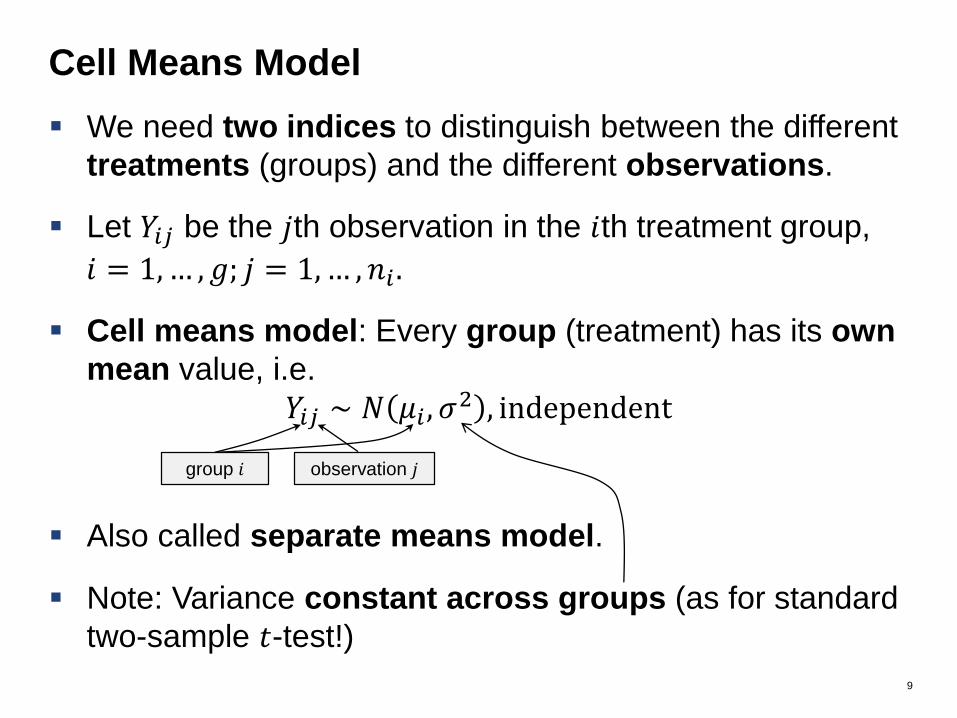
We need two indices to distinguish between the different

treatments (groups) and the different observations.

Let 𝑌𝑖𝑗 be the 𝑗th observation in the 𝑖th treatment group,

𝑖 = 1,… , 𝑔; 𝑗 = 1,… , 𝑛𝑖 .

Cell means model: Every group (treatment) has its own

mean value, i.e.

𝑌𝑖𝑗 ∼ 𝑁 𝜇𝑖 , 𝜎2 , independent

Also called separate means model.

Note: Variance constant across groups (as for standard

two-sample 𝑡-test!)

9

Cell Means Model

group 𝑖 observation 𝑗

See R-Code: 02_model_illustration.R

Or visit

https://gallery.shinyapps.io/anova_shiny_rstudio/

Why cell means? Have a look at meat storage data:

10

Illustration of Cell Means Model

Commercial Vacuum Mixed CO2

7.66

6.98

7.80

5.26

5.44

5.80

7.41

7.33

7.04

3.51

2.91

3.66

cell

We can “extract” the deterministic part in 𝑌𝑖𝑗 ∼ 𝑁(𝜇𝑖 , 𝜎2).

Leads to

𝑌𝑖𝑗 = 𝜇𝑖 + 𝜖𝑖𝑗

with 𝜖𝑖𝑗 i. i. d. ∼ 𝑁 0, 𝜎2 .

The 𝜖𝑖𝑗 ’s are random “errors” that fluctuate around zero.

In the regression context: 𝑌 is the response.

Treatment is a categorical predictor (a factor).

Hence, this is nothing else than a regression model with a

categorical predictor.

11

Cell Means Model: Alternative Representation

We can also write 𝜇𝑖 = 𝜇 + 𝛼𝑖 , 𝑖 = 1,… , 𝑔.

E.g., think of 𝜇 as a “global mean” and 𝛼𝑖 as the

corresponding deviation from the global mean.

𝛼𝑖 is also called the 𝑖th treatment effect.

This looks like a needless complication now, but will be

very useful later (with factorial treatment structure).

Unfortunately this model is not identifiable anymore.

Reason: 𝑔 + 1 parameters (𝜇, 𝛼1, … , 𝛼𝑔) for 𝑔 different

means…

12

Yet Another Representation (!)

Need side constraint: many options available.

Sum of the treatment effects is zero, i.e.

𝛼𝑔 = − 𝛼1 + ⋯𝛼𝑔−1

(R: contr.sum)

Sum of weighted treatment effects is zero: …

(R: do manually)

Set 𝜇 = 𝜇1, hence 𝛼1 = 0, 𝛼2 = 𝜇2 − 𝜇1, 𝛼3 = 𝜇3 − 𝜇1, …

i.e. a comparison with group 1 as reference level.(R: contr.treatment)

Only 𝑔 − 1 elements of the treatments effect are allowed to

vary freely. We also say that the treatment effect has 𝑔 − 1degrees of freedom (df).

13

Ensuring Identifiability

The encoding scheme (i.e., the side constraint being used)

of a factor is called contrast in R.

To summarize: we have a total of 𝑔 parameters:

𝜇, 𝛼1, … , 𝛼𝑔−1 to parametrize the 𝑔 group means 𝜇1, … , 𝜇𝑔.

The interpretation of the parameters 𝜇, 𝛼1, … , 𝛼𝑔−1 strongly

depends on the parametrization that is being used.

We will re-discover the word “contrast” in a different way

later…

14

Encoding Scheme of Factors

Choose parameter estimates 𝜇, 𝛼1, … , 𝛼𝑔−1 such that

model fits the data “well”.

Criterion: Choose parameter estimates such that

𝑖=1𝑔

𝑗=1𝑛𝑖 𝑦𝑖𝑗 − 𝜇 − 𝛼𝑖

2

is minimal (so called least squares criterion, exactly as

in regression).

The estimated cell means are simply

𝜇𝑖 = 𝜇 + 𝛼𝑖

15

Parameter Estimation

See blackboard (incl. definition of residual)

16

Illustration of Goodness of Fit

Rule: If we replace an index with a dot (“⋅”) it means that we

are summing up values over that index.17

Some Notation

Symbol Meaning Formula

𝑦𝑖⋅ Sum of all values in group 𝒊 𝑦𝑖⋅ =

𝑗=1

𝑛𝑖

𝑦𝑖𝑗

𝑦𝑖⋅ Sample average in group 𝒊 𝑦𝑖⋅ =1

𝑛𝑖

𝑗=1

𝑛𝑖

𝑦𝑖𝑗 =1

𝑛𝑖𝑦𝑖⋅

𝑦⋅⋅ Sum of all observations 𝑦⋅⋅ =

𝑖=1

𝑔

𝑗=1

𝑛𝑖

𝑦𝑖𝑗

𝑦⋅⋅ Grand mean 𝑦⋅⋅ =𝑦⋅⋅

𝑁

“Obviously”, the 𝜇𝑖’s that minimize the least squares

criterion are 𝜇𝑖 = 𝑦𝑖⋅.

Means: Expectation of group 𝑖 is estimated with sample

mean of group 𝑖.

The 𝛼𝑖′𝑠 are then simply estimated by applying the

corresponding parametrization, i.e.

𝛼𝑖 = 𝜇𝑖 − 𝜇 = 𝑦𝑖⋅ − 𝑦⋅⋅

18

Parameter Estimates, the Other Way Round

The fitted values 𝜇𝑖 (and the residuals) are

independent of the parametrization, but the

𝛼𝑖’s (heavily) depend on it!

We denote residual (or error) sum of squares by

𝑆𝑆𝐸 = 𝑖=1𝑔

𝑗=1𝑛𝑖 𝑦𝑖𝑗 − 𝑦𝑖⋅

2

Estimator for 𝜎2 is 𝑀𝑆𝐸, mean squared error, i.e.

𝜎2 = 𝑀𝑆𝐸 =1

𝑁−𝑔𝑆𝑆𝐸 =

1

𝑁−𝑔 𝑖=1

𝑔𝑛𝑖 − 1 𝑠𝑖

2

This is an unbiased estimator for 𝜎2 (reason for 𝑁 − 𝑔instead of 𝑁 in the denominator).

We also say that the error estimate has 𝑁 − 𝑔 degrees of

freedom (𝑁 observations, 𝑔 parameters) or

𝑁 − 𝑔 = 𝑖=1𝑔

(𝑛𝑖 − 1 ).

19

Parameter Estimation

empirical variance

in group 𝑖

Standard errors for the parameters (using the sum of

weighted treatment effects constraint)

Therefore, a 95% confidence interval for 𝛼𝑖 is given by

𝛼𝑖 ± 𝑡𝑁−𝑔0.975 ⋅ 𝜎

1

𝑛𝑖−

1

𝑁

20

Estimation Accuracy

Parameter Estimator Standard Error

𝜇 𝑦⋅⋅ 𝜎/ 𝑁

𝜇𝑖 𝑦𝑖⋅ 𝜎/ 𝑛𝑖

𝛼𝑖 𝑦𝑖⋅ − 𝑦⋅⋅ 𝜎1

𝑛𝑖−

1

𝑁

𝜇𝑖 − 𝜇𝑗 = 𝛼𝑖 − 𝛼𝑗 𝑦𝑖⋅ − 𝑦𝑗⋅ 𝜎1

𝑛𝑖+

1

𝑛𝑗

97.5% quantile of 𝑡𝑁−𝑔 distribution𝑁 − 𝑔 degrees of freedom because of

degrees of freedom of 𝑀𝑆𝐸

Extending the null-hypothesis of the 𝑡-test to the situation

where 𝑔 > 2, we can (for example) use the (very strong)

null-hypothesis that treatment has no effect on the

response.

In such a setting, all values (also across different

treatments) fluctuate around the same “global” mean 𝜇.

Model reduces to: 𝑌𝑖𝑗 i. i. d. ∼ 𝑁(𝜇, 𝜎2)

Or equivalently: 𝑌𝑖𝑗 = 𝜇 + 𝜖𝑖𝑗 , 𝜖𝑖𝑗 i. i. d. ∼ 𝑁 0, 𝜎2 .

This is the single mean model.

21

Single Mean Model

Note: Models are “nested”, single mean model is a

special case of cell means model.

Or: Cell means model is more flexible than single mean

model.

Which one to choose? Let a statistical test decide.

22

Comparison of models

Cell means model

Single mean model

Classical approach: decompose “variability” of response

into different “sources” and compare them.

More modern view: Compare (nested) models.

In both approaches: Use statistical test with global null

hypothesis

versus the alternative

𝐻0 says that the single mean model is ok.

𝐻0 is equivalent to 𝛼1 = 𝛼2 = … = 𝛼𝑔 = 0.

23

Analysis of Variance (ANOVA)

𝐻0: 𝜇1 = 𝜇2 = ⋯ = 𝜇𝑔

𝐻𝐴: 𝜇𝑘 ≠ 𝜇𝑙 for at least one pair 𝑘 ≠ 𝑙

See blackboard.

24

Decomposition of Total Variability

25

Illustration of Different Sources of Variability

CO2 Commercial Mixed Vacuum

34

56

7

y

-

- -

-Between groups (“signal”)

Within groups (“noise”)Grand mean

26

ANOVA table

Present different sources of variation in a so called

ANOVA table:

Use 𝑭-ratio (last column) to construct a statistical test.

Idea: Variation between groups should be substantially

larger than variation within groups in order to reject 𝐻0.

This is a so called one-way ANOVA.

Source df Sum of squares (SS) Mean Squares (MS) F-ratio

Treatments 𝑔 − 1 𝑆𝑆𝑇𝑟𝑡 𝑀𝑆𝑇𝑟𝑡 =𝑆𝑆𝑇𝑟𝑡

𝑔−1

𝑀𝑆𝑇𝑟𝑡

𝑀𝑆𝐸

Error 𝑁 − 𝑔 𝑆𝑆𝐸 𝑀𝑆𝐸 =𝑆𝑆𝐸

𝑁 − 𝑔

because only one factor involved

It can be shown that 𝐸 𝑀𝑆𝑇𝑟𝑡 = 𝜎2 + 𝑖=1𝑔

𝑛𝑖𝛼𝑖2/(𝑔 − 1)

Hence under 𝐻0: 𝑀𝑆𝑇𝑟𝑡 is also an estimator for 𝜎2

(contains no “signal” just “error”).

Therefore, under 𝐻0: 𝐹 =𝑀𝑆𝑇𝑟𝑡

𝑀𝑆𝐸≈ 1.

If we observe a value of 𝐹 that is “much larger” than 1,

we will reject 𝐻0.

What does “much larger” mean here?

We need to be more precise: we need the distribution of

𝐹 under 𝐻0.

27

More Details about the 𝐹-Ratio

Under 𝐻0 it holds that 𝐹 follows a so called 𝑭-distribution

with 𝑔 − 1 and 𝑁 − 𝑔 degrees of freedom: 𝐹𝑔−1, 𝑁−𝑔.

The 𝑭-distribution has two degrees of freedom

parameters: one from the numerator and one from the

denominator mean square (treatment and error).

Technically: 𝐹𝑛, 𝑚 =1

𝑛(𝑋1

2+⋯𝑋𝑛2)

1

𝑚(𝑌1

2+⋯𝑌𝑚2 )

where 𝑋𝑖 , 𝑌𝑗 are i.i.d. 𝑁(0,1).

Illustration and behaviour of quantiles: see R-Code.

We reject 𝐻0 if the corresponding 𝒑-value is small enough

or if 𝐹 is larger than the corresponding quantile (the 𝐹-test

is always a one-sided test).

28

𝐹-Distribution

It holds that 𝐹1,𝑛 = 𝑡𝑛2 (the square of a 𝑡𝑛-distribution)

It can be shown that the 𝐹-test for the 𝑔 = 2 case is

nothing else than the squared 𝑡-test.

The 𝐹-test is also called an omnibus test (Latin for "for

all“) as it compares all group means simultaneously.

29

More on the 𝐹-Test

Use function aov to perform “analysis of variance”

When calling summary on the fitted object, an ANOVA

table is printed out.

30

Analysis of Meat Storage Data in R

Reject 𝐻0 because p-

value is very small

Coefficients can be extracted using the function coef or

dummy.coef

Compare with fitted values (see R-Code).31

Analysis of Meat Storage Data in R

Useless if encoding

scheme unknown.

Interpretation for

computer trivial.

For you?

Coefficients in terms of

the original levels of the

coefficients rather than

the “coded” variables.

𝜇CO2= 5.9 − 2.54 = 3.36

𝜇Commercial = 5.9 + 1.58 = 7.48𝜇Mixed = 5.9 + 1.36 = 7.26

𝜇Vacuum = 5.9 − 0.40 = 5.50

Because 𝑆𝑆𝑇 = 𝑆𝑆𝑇𝑟𝑡 + 𝑆𝑆𝐸 we can rewrite the nominator

of the 𝐹-ratio as

(𝑆𝑆𝑇 − 𝑆𝑆𝐸)/(𝑔 − 1)

Or in other words, 𝑆𝑆𝑇𝑟𝑡 is the reduction in residual sum

of squares when going from the single mean to cell

means model.

If we reject the 𝐹-test, we conclude that we really need

the more complex cell means model.

32

ANOVA as Model Comparison

Residual sum of squares of

single mean model

Residual sum of squares of

cell means modelDifference in number of

model parameters

Statistical inference (e.g., 𝐹-test) is only valid if the model

assumptions are fulfilled.

Need to check

Are the errors normally distributed?

Are the errors independent?

Is the error variance constant?

We don’t observe the errors but we have the residuals as

proxy.

Will use graphical assessments to check assumptions. QQ-Plot

Tukey-Anscombe plot (TA plot)

Index plot

…

33

Checking Model Assumptions

Plot empirical quantiles of residuals vs. theoretical

quantiles (of standard normal distribution).

Points should lie more or less on a straight line if

residuals are normally distributed.

R: plot(fit, which = 2)

If unsure, compare with (multiple) simulated versions from

normal distribution with the same sample size

qqnorm(rnorm(nrow(data))

Outliers can show up as isolated points in the “corners”.

34

QQ-Plot (is normal distribution good approximation?)

35

QQ-Plot (Meat Storage Data)

-1.5 -1.0 -0.5 0.0 0.5 1.0 1.5

-1.5

-0.5

0.5

Theoretical Quantiles

Sta

nd

ard

ize

d r

esid

ua

ls

aov(y ~ treatment)

Normal Q-Q

211

3

Plot residuals vs. fitted values

Checks homogeneity of variance and systematic bias

(here not relevant yet, why?)

R: plot(fit, which = 1)

“Stripes” are due to the data structure (𝑔 different groups)

36

Tukey-Anscombe Plot (TA-Plot)

37

Tukey-Anscombe Plot (Meat Storage Data)

4 5 6 7

-0.6

-0.4

-0.2

0.0

0.2

0.4

Fitted values

Re

sid

ua

ls

aov(y ~ treatment)

Residuals vs Fitted

211

3

38

Constant Variance?

2 4 6 8 10 12 14

-1.5

-0.5

0.0

0.5

1.0

1.5

Group

Re

sid

ua

l

Plot residuals against time index to check for potential

serial correlation (i.e., dependence with respect to time).

Check if results close in time too similar / dissimilar?

Similarly for potential spatial dependence.

39

Index Plot

Transformation of response (square root, logarithm, …)

to improve QQ-Plot and constant variance assumption.

Carefully inspect potential outliers. These are very

interesting and informative data points.

Deviation from normality less problematic for large

sample sizes (reason: central limit theorem).

Extend model (e.g., allow for some dependency

structure, different variances, …)

Many more options…

More details: Exercises and Oehlert (2000), Chapter 6.

40

Fixing Problems