Complex dynamics of a unidirectional optical oscillator based on a liquid-crystal gain medium

A. Montina,1 U. Bortolozzo,2 S. Residori,3 J. P. Huignard,4 and F. T. Arecchi11Dipartimento di Fisica, Università di Firenze, Via Sansone 1, 50019 Sesto Fiorentino, Firenze Italy

2Laboratoire de Physique Statistique de l’ENS, 24 rue Lhomond, 75231 Paris Cedex 5, France3INLN, CNRS, Université de Nice Sophia-Antipolis, 1361 route des Lucioles, 06560 Valbonne, France

4Thales Research and Technology, RD 128 91767 Palaiseau Cedex, France�Received 17 July 2007; published 24 September 2007�

A unidirectional optical oscillator consists of an optical amplifier whose outgoing field is reinjected into theincoming one by means of a ring cavity. We used recently a liquid crystal light valve as optical amplifier andreported experimental evidence of cavity field oscillations. The light-valve provides a high gain and a widetransverse size, activating a large number of cavity modes, both transverse and longitudinal. A mean-fieldapproximation along the cavity axis is not suitable for this system, thus we introduce a model which accountsfor the activation of different transverse and longitudinal modes and shows numerically that their interactiongenerates three-dimensional spatiotemporal pulses localized along the cavity axis. The generation of thesepulses is experimentally verified.

DOI: 10.1103/PhysRevA.76.033826 PACS number�s�: 42.65.Sf, 05.45.�a, 42.70.Df, 61.30.�v

I. INTRODUCTION

A laser is a positive feedback optical amplifier. The activemedium with population inversion acts as the light amplifierby means of stimulated emission and the cavity supplies thefeedback �1�. The two-wave mixing �2WM� in nonlinearphotorefractive crystals provides another mechanism of lightamplification �2� and has been intensively used to observe arich variety of spatiotemporal dynamics of the transversecavity modes �3�. Because of the limited transverse size ofphotorefractive crystals, the number of activated modes isrelatively small, typically about few tens. Recently, we pro-vided experimental evidence of optical oscillations with ahuge number of modes using a liquid crystal light valve�LCLV� as the two-wave mixing device �4�.

In this paper we present the full derivation of the modelfor the unidirectional optical oscillator based on the LCLV asthe gain medium. Experimental results, such as the three-dimensional �3D� spatiotemporal pulses, are presented andcompared to the theoretical predictions. The model is derivedstarting from the Maxwell equations for the light propagationin the cavity and from the theory of the LCLV. The maindifferences with respect to existing models of cavity oscilla-tors �5–7� are due to the specific features of the gain medium.Indeed, due to the large gain and transverse size of theLCLV, a huge number of transverse and longitudinal modescan be simultaneously activated, preventing the use of amean-field approximation along the cavity axis. Thus, ourmodel considers the effects of different longitudinal modesand accounts for longitudinal variations of the cavity field.We show that the field displays spatiotemporal pulses local-ized in the transverse and longitudinal directions. Anotherimportant difference with previous models for photorefrac-tive ring cavities is the second-order nonlinear coefficient ofthe refractive index; in photorefractive media it is generallyimaginary, but for the LCLV it is always real. This has im-portant consequences on the saturation mechanisms and thedynamical interplay among different modes.

In Sec. II, we give a brief description of the experimentalsetup. In Sec. III, we introduce the equations for the LCLV

and the cavity field. In Sec. IV we analyze the model in theone-mode approximation and recover the mean-field ap-proximation in the limit of a suitably small number ofmodes. In Sec. V, simulations are presented for a one trans-verse dimension and a large number of modes, showing thepresence of a longitudinal pattern of the cavity field. In Sec.VI, we report the experimental data and provide evidence oflongitudinal multimode effects. Finally, in Sec. VII we givethe conclusions. Five movies of both numerical and experi-mental dynamics are available online �8�. Their descriptionwill be given in Secs. V and VI.

II. DESCRIPTION OF THE EXPERIMENTAL SETUP

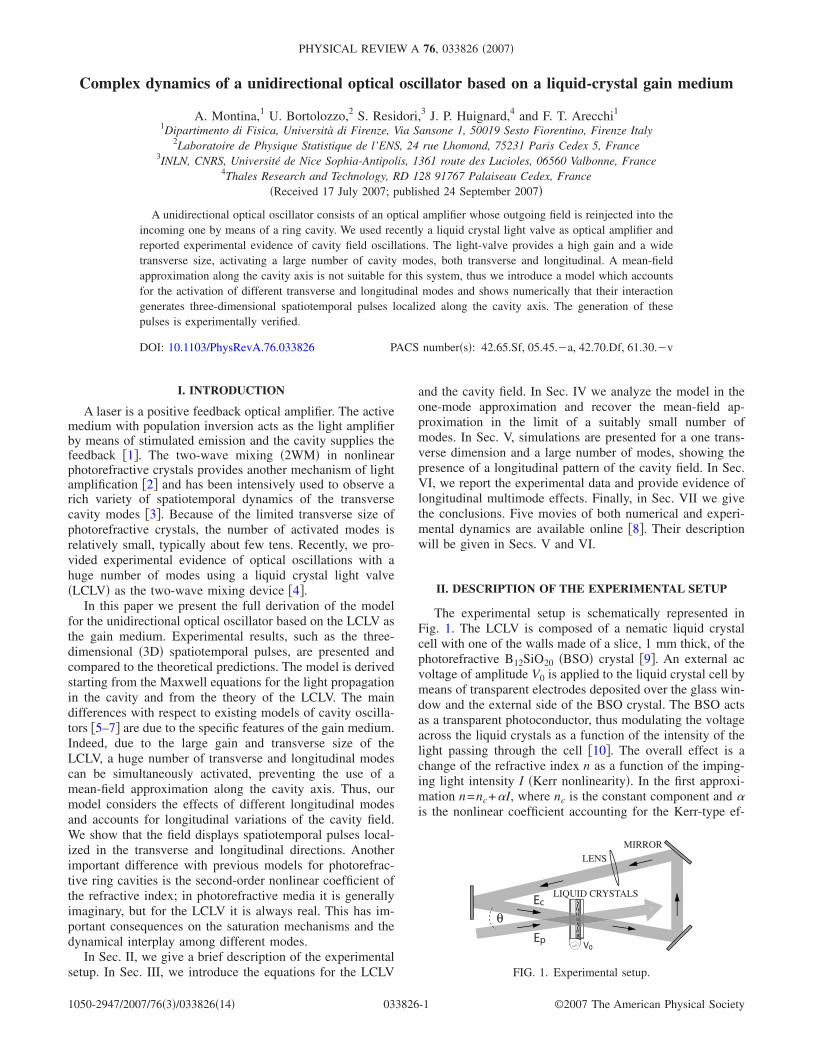
The experimental setup is schematically represented inFig. 1. The LCLV is composed of a nematic liquid crystalcell with one of the walls made of a slice, 1 mm thick, of thephotorefractive B12SiO20 �BSO� crystal �9�. An external acvoltage of amplitude V0 is applied to the liquid crystal cell bymeans of transparent electrodes deposited over the glass win-dow and the external side of the BSO crystal. The BSO actsas a transparent photoconductor, thus modulating the voltageacross the liquid crystals as a function of the intensity of thelight passing through the cell �10�. The overall effect is achange of the refractive index n as a function of the imping-ing light intensity I �Kerr nonlinearity�. In the first approxi-mation n=nc+�I, where nc is the constant component and �is the nonlinear coefficient accounting for the Kerr-type ef-

LENS

LIQUID CRYSTALS

θ

MIRROR

V0Ep

Ec

FIG. 1. Experimental setup.

PHYSICAL REVIEW A 76, 033826 �2007�

1050-2947/2007/76�3�/033826�14� ©2007 The American Physical Society033826-1

fect. The advantages of the LCLV with respect to other non-linear media are the high value of � and the large transversesize �in our valve the cell area is 20�30 mm2�, allowing thesimultaneous amplification of a large number of cavitymodes, both transverse and longitudinal.

The LCLV is positioned inside a ring cavity consisting ofthree high-reflectivity dielectric mirrors. A lens with focallength f is inserted in the cavity in order to fulfill the stabilitycondition 4f �Lcav and have a discrete spectrum for thetransverse modes. The total length of the cavity is Lcav=240 cm and the lens has a f =70 cm focal length. TheLCLV is pumped by a plane-wave optical beam provided bya diode pumped solid state laser ��=532 nm� and propagat-ing at an angle ��30 mrad with respect to the cavity axis.

The light amplification in the cavity is based on two-wavemixing interactions in the liquid crystals �9�. The pump po-larization is linear and parallel to the liquid crystal directororientation, which is vertical. The pump induces in the liquidcrystal a homogeneous variation of the refractive indexn�r���, r�� being the transverse coordinates of the two-dimensional layer. Because of inhomogeneous thermal fluc-tuations of n�r���, a small fraction of light is scattered in thedirection of the cavity axis and, after a turn in the ring, itadds to the pump field creating a small grating in n�r���. Ifthe losses in the cavity are sufficiently small, this gratingscatters a larger fraction of the pump field into the ring andan exponential growth of the cavity field occurs, until satu-ration effects become relevant. The spontaneously generatedcavity field is polarized along the vertical direction, sinceonly the extraordinary waves are amplified by the 2WM �9�.

The Fresnel number of the cavity, which is the ratio of thediffraction limiting aperture to the area of the fundamentalGaussian mode, is controlled by a diaphragm placed behindthe lens and can be changed from F=1 to approximately F=500, which implies changing from a single transverse modeoscillation to a regime where a huge number of modes areinteracting. The number of oscillating modes can be changedalso by varying the voltage V0 applied to the LCLV. Indeed,V0 changes the uniform refractive index of the LCLV, thus itacts directly on the frequency detuning between the cavityfield and the pump beam, which, as we will see in the fol-lowing, is the main mechanism of mode selection.

For the purpose of visualization, a small fraction �4%� ofthe cavity field is extracted by a beam sampler and, afterpassing through a lens, is separated into three distinct opticalpaths. Three charge-coupled device CCD cameras record thetransverse intensity distributions at three different planes,chosen in such a way to image the cavity field at three dif-ferent planes situated at different z coordinates along thecavity axis.

III. THEORY OF THE MANY-MODE LIQUID CRYSTALOSCILLATOR

In Sec. III A we study the two-wave mixing interaction inthe LCLV and show that it provides an amplification mecha-nism when one of the fields is much larger than the otherone. In Sec. III B, we complete the model of the liquid crys-

tal optical oscillator �LCO� introducing the equations for thering cavity feedback.

The model is derived by coupling the Maxwell equationswith a Debye relaxation equation for the refractive index inthe liquid crystal layer. We anticipate that we will end upwith two medium equations, one for the slowly varying com-ponent of the refractive index, describing the self-interactionof the cavity field, and one for the spatial grating, giving the2WM mechanism of photon injection inside the cavity. Thedynamics of the refractive index depends on the field inten-sity impinging on the photoconductor side of the LCLV, thusthe two medium equations are coupled to an evolution equa-tion for the cavity field, which accounts also for the longitu-dinal variations along the propagation direction. Because ofthe large scale separation between the liquid crystal responsetime and the light round-trip time in the cavity, the fieldevolution is slaved to that of the refractive index. In Appen-dix A we describe a numerical method that efficiently solvesthe cavity field equation.

A. The LCLV as a light amplifier

Let r��, z be the transverse and normal coordinates of theliquid crystal layer, respectively. The origin of z is positionedat the entrance side of the liquid crystal layer. In a widerange of parameters, the LCLV is characterized by a nearlyconstant coefficient �. Thus, for a constant impinging lightintensity I�r���, the uniform refractive index is n�r���=nc

+�I�r���. Because of the finite relaxation time � and thecharge carrier diffusion in the photoconductor layer, fortime-dependent I the refractive index obeys the followingrelaxation equation:

�n�r��,t� = �− 1 + l02��

2 �n�r��,t� + �I�r��,t� + nc, �1�

where l0 is the diffusion length of the charge carriers �11�.Let the impinging light be the superposition of a strong

pump beam and a weak one with wave numbers k�p and k�c,respectively. The angle � between them is small and they arenearly orthogonal to the LCLV. We take a plane pump waveand write the overall electric field as follows:

E�r�,t� = Epei�k�p·r�−�pt� + Ec�r�,t�ei�k�c·r�−�pt� �z 0� , �2�

where Ep is a constant amplitude and Ec is slowly varying intime and space with respect to the carrier ei�k�cr�−�p·t�, with�p�c �k�p � �c �k�c�.

The light intensity arriving at the photoconductive side ofthe LCLV is

�E�r�,t��2 = �Ep�2 + �Ec�r�,t��2 + �Ep*Ec�r�,t�e−iK� �·r� + c.c.� ,

�3�

where K� ��k�p−k�c, which is nearly parallel to the liquid crys-tal layer. The first two terms generate a slowly varying re-fractive index, whereas the last one produces a grating with

wave number K� �. If the spatial spectral width of Ec is suffi-

ciently smaller than �K� ��, the refractive index can be decom-posed as

MONTINA et al. PHYSICAL REVIEW A 76, 033826 �2007�

033826-2

n�r��,t� = n + n0�r��,t� + �n1�r��,t�e−iK� �·r�� + c.c.� , �4�

where n�nc+�Ip is a constant term, Ip��Ep�in��2 being the

pump intensity at the entrance of the LCLV �z=0�. Replacingthis equation into Eq. �1�, we obtain the equations for theenvelope fields n0 and n1,

�n0 = �− 1 + l02��

2 �n0 + ��Ec�in��r��,t��2, �5�

�n1 = �− c1 − 2il02K� � · �� � + l0

2��2 �n1 + �Ep

�in�*Ec�in��r��,t� ,

�6�

where Ec�in��r�� , t� is the cavity field at z=0 �entrance side of

the LCLV� and c1�1+ l02�K� ��2.

Now, we must evaluate the outgoing fields. If the higherscattering orders are negligible, the main effect of the modu-lation of the refractive index consists in coupling Ep and Ec.A photon in the pump beam can scatter into the cavity fieldand vice versa. However, if �k�p�d�n1� is not much smaller than2, multiple scatterings into higher orders occur and a pho-ton can acquire a transverse wave number which is a mul-

tiple of K� �, as schematically depicted in Fig. 2. Because ofthe high gain of the LCLV, we must account for these higherorder scatterings and write the field in the liquid crystal asfollows:

E�r�,t� = ei�nk�p·r�−�pt� �m=−�

�

Em�r�,t�e−imK� �·r� �z � 0� , �7�

where m is the order of the scattered wave. At z=0, E0

=Ep�in�, E1=Ec

�in� and the other components are zero. Note thatwe have multiplied the wave number k�p by the uniform re-fractive index n.

In order to fulfill the continuity condition of E and itsderivative at the boundary between regions with differentrefractive index, we should account for reflections. Howevertheir effect can be included in the overall losses, which weneglect for the moment. The electric field E in the liquidcrystal satisfies the equation

�2E�r�,t� −n2�r��

c2

�2E�r�,t��t2 = 0. �8�

We assume that the component Ec is nearly constant withrespect to the optical frequency and neglect the time depen-dence of the components Em �adiabatic approximation�. Fur-thermore, the small thickness of the liquid crystal layer and

smallness of n0 and n1 enable us to neglect the diffractiveterms �2Em and the squares n0

2 and n12. Since only the first

scattering orders are relevant, we can assume the vectors

k�p−mK� � nearly parallel to k�p in the terms with the gradientof Ec. With these approximations, Eq. �8� becomes

�Em�r��,z��z

= ik �l=−1

1

nlEm−l�r��,z� , �9�

where k��k�p���k�c�. The eigenmodes are Em�s��r���

=F�s��r���eism, where s� �0,2� and F is a complex function.The corresponding eigenvalues are

��s��r��� � ik �l=−1

1

nl�r���e−ils. �10�

The general solution of Eq. �9� is

Em�r��,z� = 0

2

dsF�s��r���e��s��r���zeism. �11�

For z=0, E0=Ep�in�, E1=Ec

�in� and the remaining componentsare zero, thus we have that

F�s��r��� =1

2�Ep

�in� + Ec�in�e−is� . �12�

By performing the integration in Eq. �11�, we find the out-going fields of Ep and Ec,

Ep�out� = ein0J0�2�n1��Ep

�in� − in1

*

�n1�J−1�2�n1��Ec

�in�� , �13�

Ec�out� = ein0J0�2�n1��Ec

�in� + in1

�n1�J1�2�n1��Ep

�in�� , �14�

where Jl are the Bessel functions of order l and where wehave introduced the rescaling of the refractive indices

kdnl → nl. �15�

In general, when there are many input fields El�in�, the

outgoing fields are

El�out� = ein0�

m�i

n1

�n1� m

Jm�2�n1��El−m�in� . �16�

The limit �n1� 1 corresponds to the first diffraction order,where photons undergo at most only one scattering process.In this limit, Eqs. �13� and �14� become �with �Ep

�in��� �Ec�in���

Ep�out� � eikn0dEp

�in�, �17�

Ecout�r��� � eikn0d�Ec

�in��r��� + ikn1dEp�in�� , �18�

where J12�2k�n1�d���k�n1�d�2 is the grating diffraction effi-

ciency in the limit of small n1.Equations �5�, �6�, and �14� are the first ingredients of the

optical oscillator model. They give the dynamics of the out-going field Ec

�out� as a function of Ec�in�. In the following sec-

tion, we consider the effect of the cavity and evaluate Ec�in� as

a function of Ec�out�.

Ep

Ec

in

in

K+2

-1

+1

0

kp

kc

kc - ks = (m-1) K(m)

FIG. 2. Multiple scatterings from the refractive index grating;ks

�m� is the wave vector of the m order scattered beam.

COMPLEX DYNAMICS OF A UNIDIRECTIONAL OPTICAL… PHYSICAL REVIEW A 76, 033826 �2007�

033826-3

In order to illustrate that the LCO can provide an ampli-fication of Ec, we consider the limit �n1� 1 and suppose thatthe incoming field Ec

�in� is much slower than n1. Thus, n1

follows adiabatically Ec�in� and can be eliminated. Neglecting

the spatial derivative in Eq. �6�, we have that n1

��Ep�in�*Ec

�in� and from Eq. �18�,

Ecout�r��� � eikn0d�1 + i�kd�Ep

�in��2�Ec�in�. �19�

Since �1+ i�kd�Ep�in��2�=�1+ ��kd�2�Ep

�in��4 is greater than 1,the LCLV acts as a light amplifier of the field Ec

�in�. Indeed,from Eq. �19� we derive the usual expression for the 2WMgain in a thin medium �10�, that is, Ic�out� / Ic�in�=1+ ��kdIp�2, where Ic= �Ec�2. It is interesting to note an impor-tant difference between the LCLV and a photorefractive crys-tal. In the latter one, � is generally an imaginary number−i�, thus its amplification factor is 1+�kd�Ep

�in��2, i.e., linearin � and for some values smaller than 1. Conversely, in theLCLV the amplification factor is quadratic in � and alwaysgreater than 1, as already pointed out in Ref. �10�.

B. Field propagation and amplification in the ring cavity

In the preceding section, we have evaluated the outgoingfields from the liquid crystal when two nearly parallel lightbeams are injected into the LCLV and shown that the deviceamplifies linearly the weaker field Ec. Now we study the casewhere this amplifier is inserted in a ring cavity, which rein-jects the field Ec

�out� into Ec�in�. When the cavity losses are

smaller than the LCLV gain and for suitable cavity detun-ings, a spontaneous growth of Ec is triggered by small ther-mal fluctuations of the refractive index, giving rise to cavityoscillations. In Eq. �14� the field Ec

�out� is a function of Ec�in�

and nk. By solving the field equation in the ring, we expressthe reinjected field Ec

�in� as a function of Ec�out�, thus eliminat-

ing the Ec�out� dependence in Eq. �14� and closing the model.

We assume Ep�in� constant in space and time. The cavity

field in vacuum satisfies the equation

��2 −1

c2

�2

�t2 Ec�r�,t�ei�k�c·r�−�pt� = 0. �20�

The carrier must be a continuous function along the ring,thus

�k�c��Lcav − d� + n�k�c�d = 2N , �21�

where N is an integer number to be chosen in such a way thatthe condition �k�c��k=�p /c is satisfied. Note that n is theuniform refractive index, which depends on the workingpoint of the LCLV through the applied voltage V0 and theinput pump intensity Ip.

If the loss rate is much larger than 1/�, we can use also inthis case the adiabatic approximation and neglect the timederivative of Ec. In the paraxial approximation we neglectthe second derivative in z of Ec and have

�Ec�r���z

= � i

2k��

2 + i��/c Ec�r�� , �22�

where ����p−c�k�c� is the frequency detuning of the Eccarrier with respect to the pump and depends on Ep by meansof n. By linearizing Eq. �21� we have

�� = ��c + n�pd

Lcav, �23�

where ��c depends on the cavity configuration and the sec-ond term is the contribution of the uniform refractive indexn=nc+��Ep

�in��2.The evolution operator through a distance L is

ei��L/cA�L� � e�iL/2k���2 +�i��L/c�. �24�

In analogy with quantum mechanics, we define an operatorwhich describes the field evolution when it passes throughthe lens. The vacuum evolution operator i

2k��2 is analogous

to the inertial operator of a nonrelativistic particle, whichcorresponds classically to the Hamiltonian 1

2k p��2 . This classi-

cal limit is equivalent to the geometrical optics limit of theMaxwell equations. A ray can be considered as the trajectoryof a particle with momentum p�� and transverse coordinater��. In our case, z corresponds to time. For rays parallel to thecavity axis, p�� is zero. The corresponding equations of mo-tion are

dr��

dz=

1

kp��, �25�

dp��

dz= 0. �26�

Their integration from z=z0 to z1 gives linear equationswhose coefficients are the ABCD matrix elements of the raytransfer matrix �12�

�1 �z1 − z0�/k0 1

�27�

�here we take the angle between the cavity axis and the ray inrad�k unit�. A lens modifies the direction of rays, i.e., thevalue of p��. This effect can be described by the equations

dr��

dz= 0, �28�

dp��

dz= − �r��, �29�

integrated over a length dL. They correspond to the Hamil-tonian �r�

2 /2. Since parallel rays are focused at the focaldistance f , we find that dL�=k / f . Thus, the field evolutionthrough the lens is described by the operator

B�f� � e�−ik/2f�r�2

, �30�

apart from an unimportant phase factor.The overall evolution operator through the ring cavity is

MONTINA et al. PHYSICAL REVIEW A 76, 033826 �2007�

033826-4

C � �1/2ei�SsmA�Lcav − L1�B�f�A�L1� , �31�

where L1 is the distance between the LCLV and the lens,

�1−�� is the fraction of lost photons in a round trip, and S isthe specular operator, sm being the number of mirrors of the

cavity. S exchanges r�� with −r�� and obviously commutes

with A and B. The phase detuning � depends on n as �see Eq.�23��

� = �c + kdn , �32�

where �c is set by the cavity. The field Ec�out� evolves through

a round trip to CEc�out�=Ec

�in�, and from Eq. �14� we obtain theequality

Cein0J0�2�n1��Ec�in� + i

n1

�n1�J1�2�n1��Ep

�in�� = Ec�in�, �33�

with C the cavity operator defined in Eq. �31�. When solvingfor Ec, we obtain

�1 − D�Ec�in��r��� = GEp

�in�, �34�

where

D � Cein0J0�2�n1�� �35�

is the operator describing the mutual coupling between thecavity modes, accounting also for losses due to scattering outof the cavity axis, and

G � Cein0in1

�n1�J1�2�n1�� �36�

is the operator accounting for the two-wave mixing processof photon injection inside the cavity. Since the eigenvalues

of D are complex numbers with modulus smaller than 1,

�1− D�−1 can be written as a Taylor series, then we have thefollowing solution for Ec

�in�:

Ec�in��r��� = �

s=0

�

DsGEp�in�. �37�

Equations �5�, �6�, and �37� constitute our model. The firsttwo equations describe the dynamics of n0 and n1 and con-tain the cavity field Ec

�in�, given by the last equation as func-tion of the refractive indices. Equation �37� has a simplephysical interpretation. The first term with s=0 gives thefield scattered by the liquid crystal into the cavity withEc

�in�=0 and its subsequent evolution through a round trip.The other terms are the contribution of this field after s re-turns to the LCLV. Because of the cavity losses, this seriesconverges and can be approximated by a finite number ofterms. The relative error with N terms is of the order of �N/2,thus with �=0.8 and 40 iterations the relative error is about1%. In Appendix A we show that it can be further reducedwhen the value of Ec

�in��t−dt� at the previous time t−dt isused as an estimate of Ec

�in��t�. The evolution given by the

cavity operator C can be numerically implemented by meansof fast Fourier transforms.

Note that the thickness of the liquid crystal layer is aparameter of the model. With the rescaling of the refractiveindices kdnl→ nl, it can be absorbed by �, defined as

� = kd� . �38�

In this way, we have eliminated in Eq. �37� the dependenceon d.

IV. ANALYSIS OF THE MODEL

In the linear regime the cavity field grows exponentiallyabove a threshold value of the pump intensity, until satura-tion terms become relevant. In Sec. IV A we analyze themodel for the LCO in the one-mode approximation evaluat-ing the threshold value and identifying the saturation mecha-nisms. In Sec. IV C we recover the familiar mean-field equa-tions under suitable conditions.

A. One-mode approximation

We assume that only one longitudinal, one transversemode of the cavity is nearly resonant and undergoes oscilla-tions. This condition can be experimentally obtained by set-ting a diaphragm inside the cavity and by closing it in such away that only the fundamental transverse mode is selected.The selection of the longitudinal mode takes place throughthe frequency detuning with respect to the pump field, as itfollows from the analysis below. In the one-mode approxi-mation the operator equation �34� is replaced by the scalarone

Ec�in� =

in1

�n1��1/2ei��0+n0�J1�2�n1��

1 − �1/2ei��0+n0�J0�2�n1��Ep

�in�, �39�

where �0 is the phase acquired by the cavity field in a roundtrip, i.e., �0c /Lcav��0 is the frequency detuning of the cav-ity mode with respect to the pump field. Let us assume thatthe eigenmode is smooth with respect to the diffusion lengthl0 and neglect the derivative terms in Eqs. �5� and �6�, whichbecome

�n0

dt= − n0 + ��Ec

�in��2, �40�

�n1

dt= − c1n1 + �Ep

�in�*Ec�in�. �41�

We now linearize Eqs. �40� and �41�, in order to study thestability of the stationary solution n0= n1=0 and find thethreshold condition for the cavity oscillation. The first equa-tion gives �dn0 /dt=−n0, thus we can take n0=0 and consideronly the second equation, which yields

�n1

dt= �− c1 + �Ip

i�1/2ei�0

1 − �1/2ei�0 n1 � c2n1. �42�

The threshold condition is Re�c2��0, i.e.,

− c1 − �Ipsin �0

1 + � − 2�1/2 cos �0� 0. �43�

The second term is an odd function of �0, is zero at �0=0,and has a maximum at

COMPLEX DYNAMICS OF A UNIDIRECTIONAL OPTICAL… PHYSICAL REVIEW A 76, 033826 �2007�

033826-5

�0M = − sgn���asin

1 − �

1 + �. �44�

With �0=�0M, the threshold value of �Ip is minimal and given

by

���Ipthr =

1 − �

�1/2 c1. �45�

As noted in Sec. III A, � is imaginary in photorefractivecrystals, thus the real part of c2 is even and has a maximumat �0=0. Conversely, in LCLV the overall gain is alwaysnegative for �0=0, since there is a phase mismatch betweenthe triggering grating n1 and the grating generated by thefeedback field. With regard to this consideration, note that inEq. �19� the outgoing field Ec

�out� is equal to the incoming oneplus a contribution with phase detuning /2, when n0=0.

For cavities with very small losses, �0M is much smaller

than 1, thus for Ip of the order of Ipthr the threshold condition

becomes

ch

c1� − 1 −

�Ip

c1

�0

�2 + �02 � 0, �46�

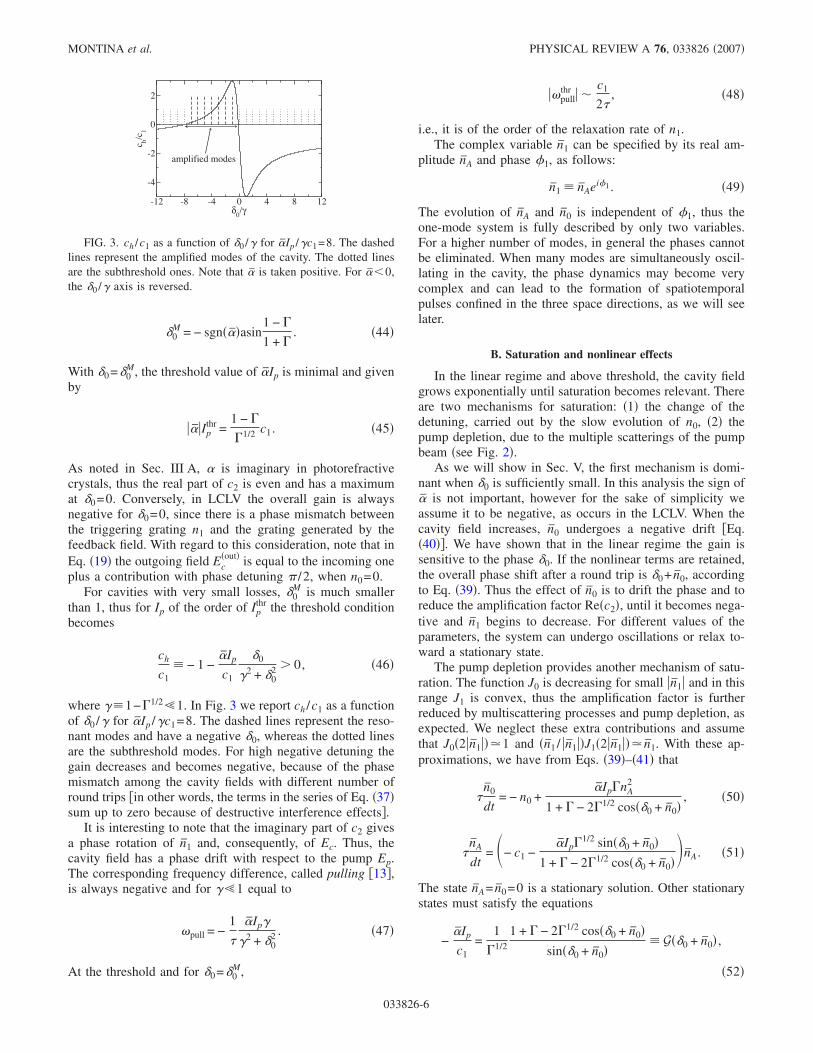
where ��1−�1/2 1. In Fig. 3 we report ch /c1 as a functionof �0 /� for �Ip /�c1=8. The dashed lines represent the reso-nant modes and have a negative �0, whereas the dotted linesare the subthreshold modes. For high negative detuning thegain decreases and becomes negative, because of the phasemismatch among the cavity fields with different number ofround trips �in other words, the terms in the series of Eq. �37�sum up to zero because of destructive interference effects�.

It is interesting to note that the imaginary part of c2 givesa phase rotation of n1 and, consequently, of Ec. Thus, thecavity field has a phase drift with respect to the pump Ep.The corresponding frequency difference, called pulling �13�,is always negative and for � 1 equal to

�pull = −1

�

�Ip�

�2 + �02 . �47�

At the threshold and for �0=�0M,

��pullthr � �

c1

2�, �48�

i.e., it is of the order of the relaxation rate of n1.The complex variable n1 can be specified by its real am-

plitude nA and phase �1, as follows:

n1 � nAei�1. �49�

The evolution of nA and n0 is independent of �1, thus theone-mode system is fully described by only two variables.For a higher number of modes, in general the phases cannotbe eliminated. When many modes are simultaneously oscil-lating in the cavity, the phase dynamics may become verycomplex and can lead to the formation of spatiotemporalpulses confined in the three space directions, as we will seelater.

B. Saturation and nonlinear effects

In the linear regime and above threshold, the cavity fieldgrows exponentially until saturation becomes relevant. Thereare two mechanisms for saturation: �1� the change of thedetuning, carried out by the slow evolution of n0, �2� thepump depletion, due to the multiple scatterings of the pumpbeam �see Fig. 2�.

As we will show in Sec. V, the first mechanism is domi-nant when �0 is sufficiently small. In this analysis the sign of� is not important, however for the sake of simplicity weassume it to be negative, as occurs in the LCLV. When thecavity field increases, n0 undergoes a negative drift �Eq.�40��. We have shown that in the linear regime the gain issensitive to the phase �0. If the nonlinear terms are retained,the overall phase shift after a round trip is �0+ n0, accordingto Eq. �39�. Thus the effect of n0 is to drift the phase and toreduce the amplification factor Re�c2�, until it becomes nega-tive and n1 begins to decrease. For different values of theparameters, the system can undergo oscillations or relax to-ward a stationary state.

The pump depletion provides another mechanism of satu-ration. The function J0 is decreasing for small �n1� and in thisrange J1 is convex, thus the amplification factor is furtherreduced by multiscattering processes and pump depletion, asexpected. We neglect these extra contributions and assumethat J0�2�n1���1 and �n1 / �n1��J1�2�n1��� n1. With these ap-proximations, we have from Eqs. �39�–�41� that

�n0

dt= − n0 +

�Ip�nA2

1 + � − 2�1/2 cos��0 + n0�, �50�

�nA

dt= �− c1 −

�Ip�1/2 sin��0 + n0�1 + � − 2�1/2 cos��0 + n0�

nA. �51�

The state nA= n0=0 is a stationary solution. Other stationarystates must satisfy the equations

−�Ip

c1=

1

�1/2

1 + � − 2�1/2 cos��0 + n0�sin��0 + n0�

� G��0 + n0� ,

�52�

-12 -8 -4 0 4 8 12δ0/γ

-4

-2

0

2

c h/c 1

amplified modes

FIG. 3. ch /c1 as a function of �0 /� for �Ip /�c1=8. The dashedlines represent the amplified modes of the cavity. The dotted linesare the subthreshold ones. Note that � is taken positive. For �0,the �0 /� axis is reversed.

MONTINA et al. PHYSICAL REVIEW A 76, 033826 �2007�

033826-6

nA2 = −

sin��0 + n0�n0

c1�1/2 . �53�

In Fig. 4 we report the phase diagram in �0 and ���Ip /c1,for �0 and �=0.85. The continuous curve represents thesolutions of Eq. �52� for n0=0 and above it the zero fieldstate is unstable, as previously shown. The minimum is at�0=�0

M and takes the value ���Ipthr /c1. �0

M and Ipthr are defined

by Eqs. �44� and �45�, respectively. It is clear that Eqs. �52�and �53� have two solutions when Ip� Ip

thr. Conversely, nosolution exists if Ip Ip

thr and the system decays always to-wards the zero cavity field state. This case corresponds to thesubthreshold region below the dotted line in Fig. 4. Note thatby changing the value of � the boundaries between the dif-ferent regions can be modified, however, the existence of theregions remains unaffected.

We determine the stability conditions for the two nonzerostationary states above the threshold Ip

thr. We linearize Eqs.�50� and �51� around the two stationary solutions and find theeigenvalues

�± = −B

2�A±

�B2 + 4An0c1�4c1 + 2A cot��0 + n0��

2�A,

�54�

where A� �Ip0 and B� A−2c1n0. n0 is one of the twononzero solutions of Eq. �52�. The product An0 being posi-tive, the stability condition Re��±�0 is satisfied if

A − 2c1n0 0,

4c1 + 2A cot��0 + n0� 0. �55�

The second inequality is satisfied if and only if 0�0+ n0�0

M. Thus, the solution with higher overall phase shift isalways a saddle node. The other one is stable if the first

inequality is satisfied. The values of ���Ip /c1 and �0 with A−2c1n0=0 are given by the following parametric equations:

�0 = q + G�q�/2,

���Ipthr/c1 = G�q� ,

0 q �0M , �56�

and they are represented by the dashed line in Fig. 4. Aboveit the system has a stable solution with nonzero cavity field.Thus, we have identified five distinct regions. The subthresh-old region is below the dotted line, where only the zero fieldsolution is stationary and every trajectory moves towards it.The �I–IV� regions are characterized by two additional sta-tionary states with nonzero field; one of them is always asaddle node. In region I the other state is stable and the zerofield configuration is unstable. In region II there is no stablesolution and the system has a stable limit cycle. The transi-tion from region I to region II takes place through a Hopfbifurcation. In region III only the zero field is a stable solu-tion. However, it is possible that in a subset of this region thesystem has a stable limit cycle, as shown in Sec. V. In thiscase we have a bistability between a fixed point and a limitcycle. In region IV the system is bistable with two stablefixed points. These different situations will be studied nu-merically in Sec. V, where we will consider also the multi-scattering processes and pump depletion.

C. Mean-field approximation

In the preceding section we have shown that near thresh-old the activated modes have a frequency detuning �0 in anarrow interval around � / tc, tc�Lcav/c being the cavityround-trip time. In this section we set the system in thisinterval and obtain under suitable conditions the mean-fieldequations.

In Appendix B, we evaluate the frequencies of the cavitymodes, that are �Eq. �B13��

�p,q,l = ���p + q� + ��l , �57�

where �� and �� are the frequency spacings of the transverseand longitudinal modes, respectively, and p, q, l are non-negative integer numbers.

The phase factor of a cavity eigenmode after a round tripis �see Eq. �31� and �B12��

Frt � e−i���p+q�tc+i�, �58�

where � is given by Eq. �32�. In Sec. IV A, we have seen thatslightly above threshold only the modes which have

Frt � e−i�ctc/2 �59�

are activated. If �ctc 1, this implies that �����p+q�tc

−��mod 2� 1. If the 2WM device has a sufficiently smalltransverse dimension, only the transverse modes with smallp and q are activated, thus

����p + q�tc − �� 1, �60�

once we assume ��� 2. In the limit of kd�n0,1� 1, we have

the following approximation for D:

0 0.2 0.4 0.6 0.8δ0

0

0.5

1

1.5

2

|α|I p/c 1

0 0.1 0.16

0.2

subthreshold region

(I) (II)

(III)

(IV)(III)

FIG. 4. Phase diagram in �0 and ���Ip /c1, for �0. The zerofield configuration is the only stationary solution below the dottedline, whereas two additional solutions are present above it. Abovethe continuous line the zero field solution becomes unstable. At theleft of the dashed line, one of the two additional solutions is stable,whereas the other one is always a saddle node. The inset shows amagnification of the bistable region �IV� close to threshold.

COMPLEX DYNAMICS OF A UNIDIRECTIONAL OPTICAL… PHYSICAL REVIEW A 76, 033826 �2007�

033826-7

D � 1 −�cLcav

2c+ i� −

iCdtc

2��

2 +iCltc

2r�

2 + ikdn0, �61�

where Cd and Cl are defined in Appendix B. Similarly, we

approximate G with ikdn1 and obtain from Eq. �34� the fol-lowing:

�−�cLcav

2c+ i� −

iCdtc

2��

2 +iCltc

2r�

2 + ikdn0 Ec = − ikdn1Ep.

�62�

In the limit of f →�, we have �Appendix B�

ic2

2�p��

2 + �i�c

Lcav−

�c

2 + i

�pd

Ln0�Ec = − i

�pd

Ln1Ep,

�63�

which is the time-independent equation of the cavity field inthe mean-field approximation and for a plane cavity �6�. It isclear that this approximation is broken when the nonlinearmedium has a large transverse dimension and the approxima-tion of Eq. �60� is no more appropriate.

V. NUMERICAL SIMULATIONS

In this section we report some numerical simulations ofthe LCO model. In Sec V A we integrate the one-mode equa-tions �50� and �51� and consider the �I–IV� regions, identifiedin the preceding section. In Sec. V B we study the multimodecase and show that the interference among the cavity modesgenerates spatiotemporal pulses.

A. One-mode simulations

In the simulations of the one-mode system we have fixedthe following parameters: �=0.15 s, �=0.85, and c1=2.58.In Fig. 5 we report the dynamics of �n0� and �n1� for �Ip /c1=0.3 and �0=0.1 �region I�. The dotted line is the stationaryvalue of n0. Note that �n1� reaches the local maxima when�n0� crosses the dotted line, i.e., when the coefficient on theright-hand side of Eq. �51� is zero. During the transient timethe refractive indices undergo damped oscillations aroundthe stationary state. This implies that the argument of the

square root in Eq. �54� is negative and the eigenvalues �± arecomplex with the real part negative.

For smaller �0 and Ip we observe that n0 collapses towardsits stationary value without oscillations. In this case the ar-gument of the square root is positive and the eigenvalues arereal and negative. This occurs, for example, with �0=0.05and �Ip /c1=0.19.

Figure 6 is the same as Fig. 5, but with �0=0.25 �regionII�. The solid and dashed lines are �n0� and �n1�, respectively.In this case there is no stable point and the dynamics be-comes oscillatory after a transient time. Note that n1 hasmaxima of the order of 0.15, thus the multiscatterings andpump depletion give relevant contributions. The dotted lineis n0, evaluated including the Bessel functions in the dynami-cal equations. With this correction there is still a stable limitcycle, but the oscillation amplitude is smaller.

In the preceding section we have shown that in region IIIonly the state with zero field is a stable stationary state.However, for some values of the parameters this state coex-ists with a stable limit cycle. In Fig. 7�a� we report �n1� as afunction of time for �Ip /c1=0.21 and �0=0.2 �region III�. Atthe initial time, �n1� is zero and stable. At a subsequent timea small pulse with Gaussian temporal shape is added to thepump field, centered at t=5 s and with the standard deviation

0

0.05

0.1

|n k|

|n1|

|n0|

0 14.03.5 7.0 10.5t /τ

FIG. 5. �n0� and �n1� as functions of time for �Ip /c1=0.3 and�0=0.1 �region I of Fig. 4�.

0

0.1

0.2

0.3

0.4

|n k|

0 14.03.5 7.0 10.5t /τ

FIG. 6. The same as Fig. 5, but with �0=0.25 �region II�. Thesolid and dashed lines are �n0� and �n1�. The dotted line is n0, evalu-ated including the Bessel functions in the dynamical equations.

0

0.05

0.1

|n 1|

0

0.04

0.08

|n 1| (b)

(a)

0 16040 80 120t /τ

FIG. 7. �n1� as a function of time, for �Ip /c1=0.21, �0=0.2 �a�and �Ip /c1=0.17, �0=0.13 �b�. In both cases a positive pulse and anegative one are added to the pump at t=5 and 27 s, respectively. In�a� �region III� we have bistability between a stable fixed point anda limit cycle. In �b� �region IV� there are two stable fixed point.

MONTINA et al. PHYSICAL REVIEW A 76, 033826 �2007�

033826-8

equal to about 0.1 s. The peak intensity variation is about30% of Ip and is sufficient to make the zero field state un-stable. This pulse carries the system into the stable limitcycle. Finally a dark pulse of the pump field is generated att=22 s and the system goes into the original state. This simu-lation has been performed including the multiscatterings andthe pump depletion. An identical behavior is obtained alsowith the approximate equations �50� and �51�.

In region IV the system has two stable fixed points, asshown in Fig. 7�b�. Also in this case we have added a posi-tive and negative pulse to the pump field at different times,but with �Ip /c1=17 and �0=0.13. After the first pulse thesystem goes into the stable state with n1�0. After the secondpulse, it returns into the original state. Also, for this simula-tion we have used in the equations the Bessel functions.They slightly change the dynamics, but the qualitative be-havior remains unchanged.

We have shown numerically the existence of different dy-namical regimes, as identified in Sec. IV by means of Eqs.�50� and �51�. The more precise inclusion of multiscatteringsand pump depletion effects change quantitatively the dynam-ics and distort the boundaries of the regions in Fig. 4, mainlyfor high �0, but the different regimes do not disappear. It isevident that the corrections are more relevant when �0 islarger, since n0 tends to counterbalance �0 so as to carry theoverall phase shift �0+ n0 to the value G−1����Ip /c1� �Eq.�52��, where the inverse of G is defined taking into consider-ation only the left branch of the continuous curve in Fig. 4.Note that the argument of the Bessel functions contains �n1�,which increases by increasing n0 �Eq. �53��.

B. Multimode simulations

We consider the multimode theory previously introducedfor the configuration of the experiment discussed in the nextsection. For the sake of simplicity, we study the case withone transverse dimension. The cavity has a length Lcav=240 cm, it is composed of three mirrors �sm=3� and a lenswith focal length f =70 cm. The pump beam is generated bya diode pumped solid state laser ��=532 nm� with an inten-sity of about 2 mW/cm2. The liquid crystal thickness d isequal to 15 �m. We assume that the fraction of lost photonsin a round trip is 25%, i.e., �=0.75, and set c1=5.5, l0=3�10−2, and �=0.15 s.

The frequency spacing of the transverse modes is givenby Eq. �B11� and in our case we have ��=96.9�106 s−1. IfL1=Lcav/2 and the liquid crystal is in the waist of the cavity,

the eigenstates of the operator C in Eq. �31� are the Hermite

functions En�x�=Hn�csx�e−�cs2x2/2�, where cs��Cd /Cl�1/4, Cd

and Cl being defined in Appendix B. If L1�Lcav/2, the

eigenstate is the evolved field En�e−�i/2k��L1−Lcav/2���2En. The

corresponding phase shift after a round trip is �n��ho�1/2+n�− /2+�, where �ho���Lcav/c=0.775 rad.

We have shown that a single mode can display differentdynamical regimes, depending on the phase shift of the fieldafter a round trip and on the pump intensity. The mode withphase shift equal to �0

M has the maximal gain. If we set �=�0

M + /2−�ho�1/2+N0�, where N0 is an integer number,

and the pump intensity is not too high, only the cavity modeN0 is triggered. In Fig. 8, we report the spatiotemporal dis-tribution of the cavity field intensity �Ec

�in��2, for N0=2 andIp=1.5Ip

thr. At the initial time the mode E2 grows and hasdamped oscillations around a stationary nonzero value, as itoccurs in the one-mode case of Fig. 5. After a transient time,higher modes are activated and a complex spatiotemporalstructure appears.

In order to clarify this behavior, we have decomposed thecavity field in eigenmodes and evaluated the mode ampli-tudes as a function of time. In Fig. 9 we report the squaredamplitudes of the cavity modes as a function of time. At theinitial times, only the mode 2 is dominant, subsequently itsamplitude decreases and seven other modes are activated.Because of the large value of �ho with respect to �, adjacentmodes cannot be simultaneously activated, but this is pos-sible for modes whose index distance is equal to 8, the cor-responding phase shift difference being 8�ho�0.987�2.Note that the modes 51 and 59 are the first activated ones,since the phase shift distance from the mode 2 is smaller thanthat of the lower modes. The higher modes are suppressedbecause of the spatial diaphragms inside the cavity. It is in-teresting to note that the jump from the low mode 2 to thehigher ones is triggered by the growing n0, which modifiesthe cavity detuning. This is another peculiarity of the LCLVwith respect to photorefractive crystals.

From Fig. 9 we see that there are eight predominantmodes, corresponding to the high intensity bands on the plot.However, in the graph are plotted the square amplitudes ofthe modes, so that even the modes represented by low levels

FIG. 8. Spatiotemporal intensity distribution of the cavity field�Ec

�in��2 for �=�0M + /2−�ho�1/2+2� and Ip=1.5Ip

thr.

FIG. 9. Squared amplitudes of the cavity modes for the dynam-ics of Fig. 8.

COMPLEX DYNAMICS OF A UNIDIRECTIONAL OPTICAL… PHYSICAL REVIEW A 76, 033826 �2007�

033826-9

of intensity cannot be neglected and they indeed participateto the dynamics. Thus, the total number of active modes isapproximately 60. An extension to a two-dimensional �2D�model will lead to approximately 3600 active modes, whichis consistent with the huge number of modes observed in theexperiment.

These results clearly show that our model accounts in anatural way for longitudinal modes and that the mean-fieldapproximation is inappropriate to describe the consideredsystem. It is valid when the phase shift differences of theactive modes are much smaller than 2. The breakdown ofthe mean-field approximation is due to both the particulargeometry of the cavity and the large transverse dimension ofthe LCLV. Its consequence is a pattern structure of the cavityfield along the z axis, as shown in Fig. 10, where we reportthe intensity distribution of the cavity field in the x-z plane.Two movies of the dynamics in the x-z plane are available�8�. The simulations in files “theory�1.mp4” and“theory�2.mp4” have been performed for Ep=7Ep

thr and Ep=5Ep

thr, respectively.

VI. EXPERIMENTAL RESULTS

The experiments were performed by using the setupshown in Fig. 1. In Fig. 11 we show a sequence of instanta-neous snapshots of the transverse intensity distributionsIc�x ,y�, where x ,y are the coordinates in the transverseplane, taken for a low Fresnel number, F=3, when the cavityfield consists of a small number of transverse modes arounda single longitudinal mode. A few low-order Gauss-Laguerremodes alternate during the time. This behavior is similar to

dynamical regimes previously observed in photorefractiveoscillators �3�. In our model, the alternation between modesis explained by the �0 shift due to the dynamics of n0. Fol-lowing the slow evolution of n0, each single mode lasts for afew seconds before changing to another one. Depending onthe control parameters, namely, the voltage V0 applied to thelight valve and the pump intensity Ip, the alternation may beperiodic or chaotic.

In the single mode regime, we have measured the fre-quency detuning between the pump and the cavity field. Thisis done by making the interference of the cavity field with areference beam having the same frequency of the pump. Thedisplacement of the interference fringes corresponds to a de-tuning, of approximately 1 Hz, which is the same for thedifferent transverse modes and corresponds to the pullingpredicted by Eq. �48�.

In a second series of experiments, we have fixed a largeFresnel number F=500, and we have investigated the dy-namical behavior of the cavity for different V0 and differentpump intensities Ip. The experimental phase diagram is re-ported in Fig. 12. Cavity field oscillations are in the largergrey area. The darker and smaller area marks the regionwhere we observe spatiotemporal pulses �4�. The low V0regimes are similar to those observed for low F, character-ized by the alternation of low-order Gauss-Laguerre modes,one pure mode at time. By changing V0 we change the uni-form refractive index of the LCLV, thus the frequency detun-ing between the fundamental Gaussian mode and the pumpfield is varied. When V0 increases, the detuning also in-creases, therefore out-of-axis emission is favored and alarger number of modes comes into play �14�. As a conse-quence, the transition to the high V0 regimes is accompaniedby the emission of high order and out-of-axis symmetricalmodes.

In Fig. 13 we show a regime where an intermediate num-ber of modes are active. The cavity field oscillations arecharacterized by the simultaneous presence of high- and low-order transverse modes, sometimes belonging to differentlongitudinal modes, as we can verify by making the interfer-ence with a reference beam and by observing different fringedisplacements in different regions of the spatial pattern. InFig. 14 we show a regime with a large number of modes butoutside the region of existence of spatiotemporal pulses. Fig-ure 14�a� displays a regime of high V0 and low Ip. In thiscase the detuning is large, so that wide ring patterns develop

FIG. 10. Intensity distribution of the cavity field in the x-z planeat t=3.5 s �a� and t=4 s �b�. Because of the activation of high ordermodes, the field is inomogeneous along z and a mean-field approxi-mation along the cavity axis is unsuitable. The lens is positioned atz=1.3 m.

a) b) c) d)

FIG. 11. Instantaneous snapshots showing the low-order Gauss-Laguerre modes alternating during the time for F=3; �a� TEM00, �b�TEM10, �c� TEM11, �d� TEM06.

FIG. 12. Experimental phase diagram in the V0 versus Ip space;G indicates the zone of low-order Gaussian modes whereas R marksthe region of wide ring patterns.

MONTINA et al. PHYSICAL REVIEW A 76, 033826 �2007�

033826-10

with depletion of the oscillations close to the cavity axis.Nevertheless, the number of active modes is large so that aspatiotemporal chaotic dynamics takes place along the ring.Figures 13�b�–13�d� correspond to a slight decrease of V0,allowing for other longitudinal modes to come into play andpopulate the central area of the pattern.

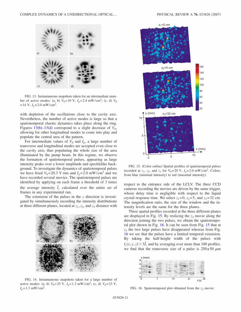
For intermediate values of V0 and Ip, a large number oftransverse and longitudinal modes are accepted even close tothe cavity axis, thus populating the whole size of the areailluminated by the pump beam. In this regime, we observethe formation of spatiotemporal pulses, appearing as largeintensity peaks over a lower amplitude and specklelike back-ground. To investigate the dynamics of spatiotemporal pulseswe have fixed V0=20.3 V rms and Ip=2.0 mW/cm2 and wehave recorded several movies. The spatiotemporal pulses areidentified by applying on each frame a threshold of 3 times

the average intensity Ic calculated over the entire set offrames in any experimental run.

The extension of the pulses in the z direction is investi-gated by simultaneously recording the intensity distributionsat three different planes, located at z1 ,z2, and z3 distance with

respect to the entrance side of the LCLV. The three CCDcameras recording the movies are driven by the same trigger,whose delay time is negligible with respect to the liquidcrystal response time. We select z1=0, z2=5, and z3=32 cm.The magnification ratio, the size of the window and the in-tensity levels are the same for the three planes.

Three spatial profiles recorded at the three different planesare displayed in Fig. 15. By reslicing the z2 movie along thedirection joining the two pulses, we obtain the spatiotempo-ral plot shown in Fig. 16. It can be seen from Fig. 15 that atz3 the two large pulses have disappeared whereas from Fig.16 we see that the pulses have a limited temporal extension.By taking the half-height width of the pulses with

Ic�x ,y ,z��3Ic and by averaging over more than 100 profiles,we find that the transverse size of a pulse is 250±50 �m

a) b)

c) d)

FIG. 13. Instantaneous snapshots taken for an intermediate num-ber of active modes: �a, b� V0=10 V, Ip=2.4 mW/cm2; �c, d� V0

=14 V, Ip=2.0 mW/cm2.

a) b)

c) d)

FIG. 14. Instantaneous snapshots taken for a large number ofactive modes: �a, b� V0=25 V, Ip=1.3 mW/cm2; �c, d� V0=23 V,Ip=1.3 mW/cm2.

x (mm)

y (mm)

160

140

120

100

80

60

40

20

0 5100

5

10

z2=5 cm

z3=32 cm

z1=0 cm

FIG. 15. �Color online� Spatial profiles of spatiotemporal pulsesrecorded at z1, z2, and z3 for V0=20 V, Ip=2.0 mW/cm2. Colors,from blue �minimal intensity� to red �maximal intensity�.

0 7 14 21 28t (s)

0

2

4

6

8x (mm)

FIG. 16. Spatiotemporal plot obtained from the z2 movie.

COMPLEX DYNAMICS OF A UNIDIRECTIONAL OPTICAL… PHYSICAL REVIEW A 76, 033826 �2007�

033826-11

whereas its average lifetime is around 0.5±0.1 s. As for thelongitudinal extension, by inspecting several movies taken atdifferent z3, we estimate it around 30 cm, which is consistentwith the results of the 2D numerical simulations.

Three experimental movies are available online �8�. Thefirst movie, recorded for V0=10 V and Ip=2.4 mW/cm2,shows the alternation among a few low-order Gaussianmodes, all belonging to the same longitudinal mode. Thesecond movie was recorded for V0=14 V and Ip=2.0 mW/cm2 and shows an increased number of transversemodes corresponding to a few different longitudinal modes.The third movie, recorded for V0=20 V and Ip=2.0 mW/cm2, corresponds to a regime when a high numberof transverse and longitudinal modes are simultaneouslypresent.

VII. CONCLUSIONS

In conclusion, we have shown that a type of nonlinearoptical oscillator can be built by using a liquid crystal lightvalve as the gain medium. We have developed a theoreticalmodel that takes into account the Kerr nonlinearity of themedium as well as the two-wave-mixing mechanism of pho-ton injection inside the cavity. At variance with the usualtreatments, where the mean-field approximation is used toeliminate the z dependence of the field, our model keeps thisdependence, thus allowing for the formation of 3D patterns.We have shown that the simultaneous presence of longitudi-nal and transverse modes leads to the appearance of spa-tiotemporal pulses, which is confirmed by numerical simula-tions and experimental results.

ACKNOWLEDGMENTS

One of the authors �U.B.� acknowledges support of theEU Contract No. MEIF-CT-2006–041594. One of the au-thors �A. M.� acknowledges support from the Ente Cassa diRisparmio di Firenze, under the project “dinamiche cerebralicaotiche.”

APPENDIX A: NUMERICAL EVALUATION OF THECAVITY FIELD

We have seen that the cavity field Ec can be evaluated asthe stationary solution of the cavity and the two-wave mixingdevice, because of the slow dynamics of the liquid crystals.Thus, Ec on the surface of the photorefractive crystal is adia-batically slaved by nk and given by Eq. �37�. In this appendixwe present a strategy to efficiently reduce the numerical er-rors due to the truncation of the series in Eq. �37�.

The operator D has eigenvalues �k with modulus equal to�1/2, � being the fraction of lost photons in each cavity roundtrip. The series is convergent since �1/21 and can be ap-proximated by a finite number N of terms.

Let us assume J0�2 � n1 � ��1 and J1�2 � n1 � �n1 / �n1 � � n1.The root-mean-square error is

ErmsR �N� �� dr���

k�s=N

�

�ksWk�2

dr���k

�s=0

�

�ksWk�2 = �N/2, �A1�

where Wk are non-normalized cavity eigenmodes, such that

�kWk= GEp. For large cavity losses, a small number of termsare necessary since many round trips of photons are improb-able. Conversely, for high qualities of the cavity, many termsof the series must be evaluated. For �=0.8 and 40 iterationsthe relative error on Ec is about 1%. This error can be furtherreduced if an estimate of Ec is known, as occurs in ourmodel. Equation �37� must be solved at every time step andEc�t� differs slightly from Ec�t−dt�, thus the previous valuecan be used as an estimate of Ec�t�. The difference betweenthe exact Ec and the sum of the first N terms is

�s=N

�

DsGEp = DN�s=0

�

DsGEp = DNEc � �N/2Ec. �A2�

Thus,

Ec = �s=0

N−1

DsGEp + DNEc, �A3�

where the second term on the right-hand side is a small cor-

rection of the order of �N/2Ec. Let Ec=Ec+O�dt� be the valueestimated at the previous time step, then we have that

Ec = �s=0

N−1

DsGEp + DNEc + �N/2O�dt� . �A4�

The second term reduces the relative error by a factor of theorder of dt. Furthermore, its evaluation increases onlyslightly the computation time, as shown by the followingalgorithm, used to solve Eq. �A4�:

K0 = GEp + DEc,

K1 = DK0 + GEp,

K2 = DK1 + GEp, … ,

Ec � KN−1 = DKN−2 + GEp. �A5�

Thus, the error reduction strategy with Eq. �A4� requires to

evaluate merely the additional term DEc in the equation forK0. More precise algorithms are obtained by second-order

estimates of Ec. In our simulations, we achieved typical pre-cisions of 10−6 with merely five terms of the series. The

operators D and G can be easily evaluated by means of fastFourier transforms, which diagonalize the differential opera-tors in the exponents.

MONTINA et al. PHYSICAL REVIEW A 76, 033826 �2007�

033826-12

APPENDIX B: CAVITY EIGENMODES

In this appendix we evaluate the cavity eigenmodes with-out the LCLV and with zero losses. They are the solutions ofthe following eigenvalue equation:

UEk = e−i�kEk, �B1�

where �k is the phase shift of the eigenmode k after a roundtrip and

U � SsmA�Lcav − L1�B�f�A�L1� . �B2�

Equation �B1� is equivalent to

USEk = e−i�kEk, �B3�

where

US � SsmA�Lcav/2�B�f�A�Lcav/2� ,

Ek = e�i�L1−Lcav/2�/2k���2Ek. �B4�

In order to find the eigenmodes, it is convenient to reduce the

operator US to the exponential of a Hermitian operator. Forsuitable values of the coefficients Cd and Cl, we have, apartfrom a unimportant phase factor,

US = e−itc��−Cd/2���2 +�Cl/2�r�

2 �, �B5�

where tc�Lcav/c is the propagation time in one round trip.The cavity with lens is equivalent to a harmonic oscillatorwith frequency ��=�CdCl. We must evaluate Cd and Cl. In

the ray limit, the operators A�Lcav/2�, B�f� and S correspond,respectively, to the following ABCD matrices of the raytransfer matrix analysis �see Sec. III B�,

A�Lcav/2� = �1 Lcav/2k

0 1 , B�f� = � 1 0

− k/f 1

S = �− 1 0

0 − 1 . �B6�

Thus, the overall unitary operator US is associated to thefollowing ABCD matrix,

US = �− 1�sm�1 −Lcav

2f

Lcav

2k�2 −

Lcav

2f

−k

f1 −

Lcav

2f� . �B7�

On the other hand, the ABCD matrix US from Eq. �B5� is

US = � cos ��tc �Cd

Clsin ��tc

−�Cl

Cdsin ��tc cos ��tc

� . �B8�

From these equations we find that

�� = sgn�hc���� −

tc��− gc� , �B9�

where

hc � 1 −Lcav

2f,

gc � �1 −Lcav

2f �− 1�sm,

�� =1

tcasin��Lcav

f�1 −

Lcav

4f , �B10�

and � is the Heaviside function. There are two interestingcases: �a� the number of mirrors sm is even and f �Lcav/2;�b� the number of mirrors is odd and Lcav/4 f Lcav/2. Inboth cases, Eq. �B9� reduces to

�� =sgn�hc�

tcasin�Lcav

f�1 −

Lcav

4f . �B11�

�� goes to zero for both f →� �plane cavity� and f

→ �Lcav/4�+ �spherical cavity�. The eigenvalues of US are

e−i�k = e−i���p+q�tc �B12�

and

�k = ����p + q� + ��l�tc, �B13�

where p, q, and l are integer numbers and �� �2c /Lcav. Thetwo terms ���p+q� and ��l are the transverse and longitu-dinal cavity frequencies. The corresponding eigenmodes arethe Gauss-Hermite functions or, equivalently, the Gauss-Laguerre functions.

The product CdCl is equal to ��2 and has been evaluated

by the diagonal elements of Eqs. �B7� and �B8�. The ratioCd /Cl can be obtained by the off-diagonal elements. In thelimit of f →�, Cd is obviously equal to Lcav/k and Cl is zero.

�1� A. E. Siegman, Lasers �Oxford University Press, Oxford,1986�.

�2� J. L. Bougrenet de la Tocnaye, P. Pellat-Finet, and J. P. Huig-nard, J. Opt. Soc. Am. B 3, 315 �1986�.

�3� F. T. Arecchi, G. Giacomelli, P. L. Ramazza, and S. Residori,Phys. Rev. Lett. 65, 2531 �1990�.

�4� U. Bortolozzo, A. Montina, F. T. Arecchi, J. P. Huignard, andS. Residori, Phys. Rev. Lett. 99, 023901 �2007�.

COMPLEX DYNAMICS OF A UNIDIRECTIONAL OPTICAL… PHYSICAL REVIEW A 76, 033826 �2007�

033826-13

�5� G. D’Alessandro, Phys. Rev. A 46, 2791 �1992�.�6� F. T. Arecchi, S. Boccaletti, G. P. Puccioni, P. L. Ramazza, and

S. Residori, Chaos 4, 491 �1994�.�7� B. M. Jost and B. E. A. Saleh, Phys. Rev. A 51, 1539 �1995�.�8� See EPAPS Document No. E-PLRAAN-76-029710 for two

numerical and three experimental movies. In the numericalones the evolution of the field intensity in the x-z plane isshown for two different values of the parameters. The experi-mental ones show the intensity field in the transverse plane forthree dynamical regimes. For more information on EPAPS, seehttp://www.aip.org/pubservs/epaps.html.

�9� U. Bortolozzo, S. Residori, and J. P. Huignard, Opt. Lett. 31,2166 �2006�.

�10� A. Brignon, I. Bongrand, B. Loiseaux, and J. P. Huignard, Opt.Lett. 22, 1855 �1997�.

�11� U. Bortolozzo, S. Residori, A. Petrosyan, and J. P. Huignard,Opt. Commun. 263, 317 �2006�.

�12� A. Yariv, Optical Waves in Crystals �Wiley, New Jersey, 2003�.�13� See, e.g., Laser Handbook, edited by T. Arecchi and E. O.

Schulz-Dubois �North-Holland, Amsterdam, 1972�.�14� U. Bortolozzo, P. Villoresi, and P. L. Ramazza, Phys. Rev. Lett.

87, 274102 �2001�.

MONTINA et al. PHYSICAL REVIEW A 76, 033826 �2007�

033826-14