Proceedings World Geothermal Congress 2015

Melbourne, Australia, 19-25 April 2015

1

Results from a Worldwide Proficiency Test on the Determination of Carbonic Species

Concentration in Natural Waters

Mahendra P. Verma1,*

, Enrique Protugal1, Sophie Gangloff

2, Ma. Aurora Arimenta

3, D. Chandrasekharam

4, Mayela

Sanchez5, Roberto E. Renderos

6, Miguel Tuanco

7, Robert van Geldern

8

1Geotermia, Instituto de Investigaciones Eléctricas, Reforma 113, Col. Palmira, Cuernavaca, Mor., C.P. 62490, Mexico.

2Laboratoire d’Hydrologie et de Géochimie de Strasbourg, Université de Strasbourg/EOST, CNRS, 1 rueBlessig, F-67000

StrasbourgCedex, France

3Instituto de Geofísica, UNAM, Circuito Exterior, C.U., México 04510 D.F.

4Department of Earth Sciences, Indian Institute of Technology Bombay, Mumbai, 400076, India.

5Dirección de Geotermia, ENEL Central Intersección de Pista Juan Pablo II y Prolongación de Avenida Bolívar, Managua-

Nicaragua

6Laboratorio Geoquímico, Gerencia de Estudios y Evaluación, LaGeo S.A. de C.V., 15 Avenida Sur, Colonia Utila Santa Tecla, La

Libertad, El Salvador, Centro America, El Salvador

7Instituto de Ciencias Agrarias CSIC C/Serrano 115 dupl 20 28006 Madrid, Spain.

8GeoZentrum Nordbayern, Applied Geosciences, Friedrich-Alexander-University Erlangen-Nuremberg, Schlossgarten 5, 91054

Erlangen, Germany

*Corresponding author’s email: mahendra@iie.org.mx

Keywords: Acid-base titration, analytical method, CO2 chemistry, inter-laboratory comparison, natural waters.

ABSTRACT

The results of an international inter-laboratory proficiency test for the determination of carbonic species concentration are

presented. Eight laboratories performed the analysis of twelve water samples (four synthetic waters, one lake water, four

geothermal waters, one seawater, and two petroleum waters) by two methods: (a) individual laboratory analytical procedure and (b)

acid-base titration curves in tabular form. From the titration curves the concentrations of carbonic species are calculated using the

Hydrologist method, Geochemist’s method and initial pH and total alkalinity method. The titration curves of all laboratories yield

very similar results (i.e., concentration of carbonic species for each sample). In contrast, the individual laboratory reported values

showed high dispersion about the mean. This implies that there are some laboratories, which have problem in their concentration

calculation procedure. To apply the Hydrologist and/or Geochemist methods it is necessary to locate always two equivalence points

(e.g., NaHCO3EP and H2CO3EP) even for samples which have pH lower than that of NaHCO3EP. In addition, the backward

titration curve with NaOH after complete removal of CO2 is strictly necessary to decide for the applicability of the Hydrologist

method or the Geochemist method. In cases where the complete analyses of species that contribute to the alkalinity are known, the

initial pH and total alkalinity method is appropriate.

1. INTRODUCTION

The geochemistry of natural systems is much more complex than that of any synthetic system studied in the laboratory. When we

extend our geochemistry knowledge acquired through laboratory experiments to natural systems, we face certain limitations.

Mankind adopts an empirical approach based on creating an analytical database for similar systems around the world. This

implicitly demands for reliable analytical measurements in every laboratory. Extensive efforts are in progress worldwide to create

reference materials (standards) for each chemical species and to calibrate analytical techniques with such materials to achieve

accuracy and consistency in the analytical database on natural geological systems.

Carbon dioxide (CO2) plays a fundamental role in governing the geological and environmental processes on Earth. The distribution

of carbonic species (H2CO3, HCO3- and CO3

2-) in natural waters permits the examination of CO2 exchange between atmosphere and

water bodies, the evaluation of buffering mechanisms and the definition of their acid-base neutralizing capacity (Stumm and

Morgan 1996). Similarly, measurements of total alkalinity and carbonic alkalinity are of great importance in analyses of ocean,

marine, lake and river waters, and other samples. The knowledge of aquatic CO2 chemistry is fundamental for the removal of

anthropogenic CO2 from atmosphere (NASA 2012), incrustation of calcite in the reservoir and production wells during geothermal

exploitation. Recently, Torres-Alvarado et al. (2012) presented the propagation of analytical uncertainty (error) in the determination

of carbonic species concentration of separated water at the weir box in the pH calculation of geothermal reservoir fluids.

Verma (2013) performed the statistical analysis of the results of inter-laboratory comparisons of chemical analysis of geothermal

waters, conducted under the quality assurance and quality control programs of International Association of Geochemistry and

Cosmochemistry (IAGC) and International Atomic Energy Agency (IAEA). There was an overall uncertainty of ±13% and

difficulty in defining the appreciable improvement in the analytical quality in the successive inter-laboratory comparisons. This is

probably due to the existence of systematic errors in the measurements from some laboratories. Specifically, there were some

problems with sampling and analytical procedures for SiO2 and HCO3-. In case of SiO2, Verma et al. (2012, 2015) found that one of

the major reasons for high dispersion in the measured values among laboratories was associated with minor differences in the

individual analytical procedures of the participating laboratories. van Geldern et al. (2013) presented an inter-laboratory

Verma et al.

2

comparison of the determination of isotopic composition (13C) of the total dissolved inorganic and organic carbon of different

types of waters.

To further investigate the analytical challenges with carbonic species analyses the present study was initiated. It consists of a

worldwide inter-laboratory comparison for the determination of carbonic species concentration in 12 water samples (four synthetic

waters, one lake water, four geothermal waters, one seawater, and two petroleum waters), distributed among eight participating

laboratories.

2. PREVIOUS INTER-LABORATORY COMPARISON FOR CARBONIC SPECIES

Ellis (1976) reported the results of first inter-laboratory comparison of chemical analysis of seven water samples, including a

geothermal water sample. However, he reported only the statistics of the dataset without the individual measured value of each

chemical parameter. The IAEA conducted a series of inter-laboratory comparisons for the chemistry of geothermal waters within

the framework of the project, “Coordinated Research Program on the Application of Isotope and Geochemical Techniques in

Geothermal Exploration” (Giggenbach et al. 1992, Gerardo-Abaya et al. 1998, Alvis-Isidro et al. 1999, 2000, 2002, Urbino and

Pang 2004) and concluded that the dispersion (scatter) in the measured values among laboratories was a consequence of water

sample alteration during transportation and storage.

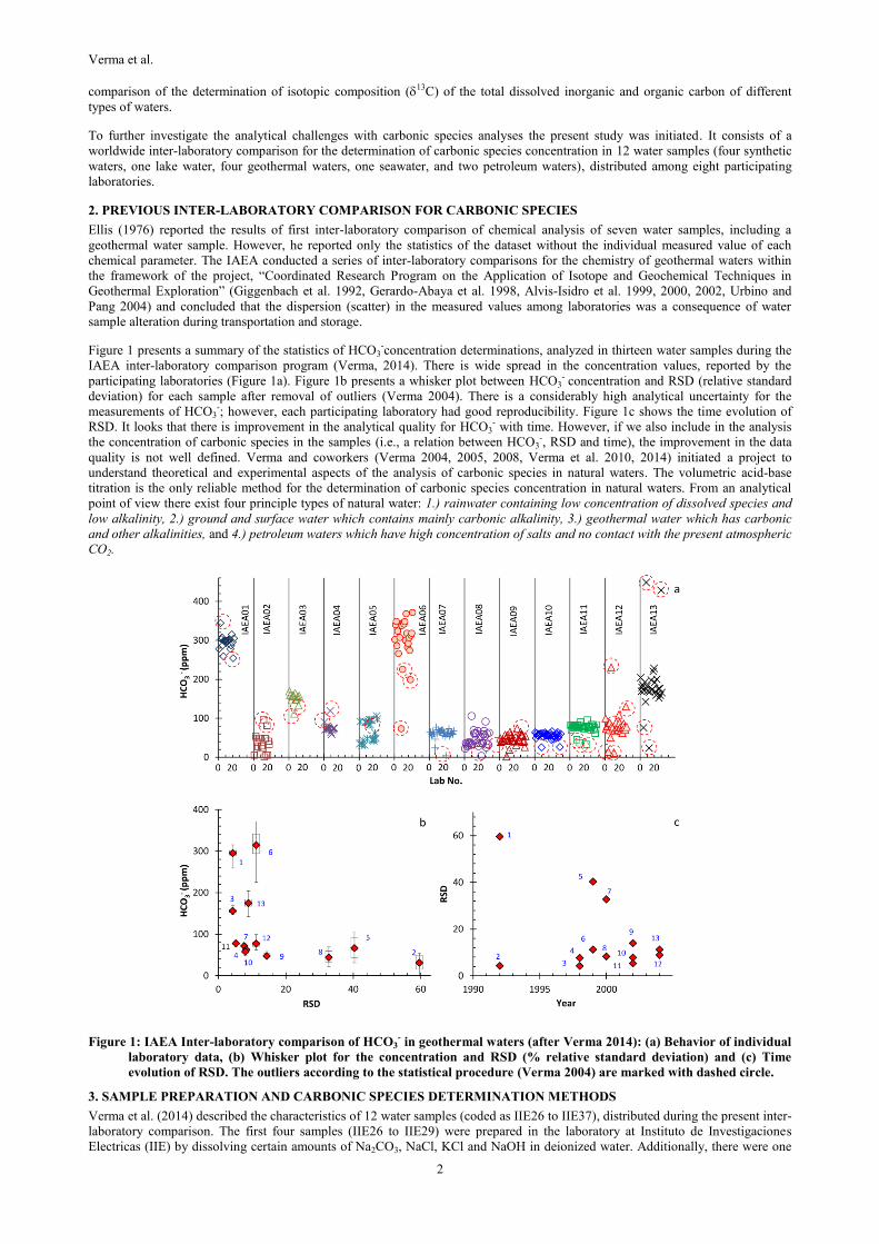
Figure 1 presents a summary of the statistics of HCO3-concentration determinations, analyzed in thirteen water samples during the

IAEA inter-laboratory comparison program (Verma, 2014). There is wide spread in the concentration values, reported by the

participating laboratories (Figure 1a). Figure 1b presents a whisker plot between HCO3- concentration and RSD (relative standard

deviation) for each sample after removal of outliers (Verma 2004). There is a considerably high analytical uncertainty for the

measurements of HCO3-; however, each participating laboratory had good reproducibility. Figure 1c shows the time evolution of

RSD. It looks that there is improvement in the analytical quality for HCO3- with time. However, if we also include in the analysis

the concentration of carbonic species in the samples (i.e., a relation between HCO3-, RSD and time), the improvement in the data

quality is not well defined. Verma and coworkers (Verma 2004, 2005, 2008, Verma et al. 2010, 2014) initiated a project to

understand theoretical and experimental aspects of the analysis of carbonic species in natural waters. The volumetric acid-base

titration is the only reliable method for the determination of carbonic species concentration in natural waters. From an analytical

point of view there exist four principle types of natural water: 1.) rainwater containing low concentration of dissolved species and

low alkalinity, 2.) ground and surface water which contains mainly carbonic alkalinity, 3.) geothermal water which has carbonic

and other alkalinities, and 4.) petroleum waters which have high concentration of salts and no contact with the present atmospheric

CO2.

Figure 1: IAEA Inter-laboratory comparison of HCO3- in geothermal waters (after Verma 2014): (a) Behavior of individual

laboratory data, (b) Whisker plot for the concentration and RSD (% relative standard deviation) and (c) Time

evolution of RSD. The outliers according to the statistical procedure (Verma 2004) are marked with dashed circle.

3. SAMPLE PREPARATION AND CARBONIC SPECIES DETERMINATION METHODS

Verma et al. (2014) described the characteristics of 12 water samples (coded as IIE26 to IIE37), distributed during the present inter-

laboratory comparison. The first four samples (IIE26 to IIE29) were prepared in the laboratory at Instituto de Investigaciones

Electricas (IIE) by dissolving certain amounts of Na2CO3, NaCl, KCl and NaOH in deionized water. Additionally, there were one

Verma et al.

3

natural lake water (IIE30), four geothermal waters (IIE31 to IIE34), one seawater (IIE35) and two petroleum waters (IIE36 and

IIE37). Each sample was filled in 250 ml Nalgene (high-density polyethylene, HDPE) bottles to distribute among the participating

laboratories. Similarly, the CO2 partial pressure of each sample was lower than the atmospheric partial pressure of CO2 and samples

were treated in the closed containers during preparation. Alteration due to the atmospheric CO2 was therefore unlikely. The sample

preparation and handling procedure was to insure the stability and homogeneity of the samples; however, no specific test was

performed to verify them.

For chemical analysis of carbonic species, each laboratory was asked to report the preparation and calibration of standards, and

analyses of the samples with two procedures: (a) regular laboratory procedure (or conventional procedure) and (b) forward and

backward titration curves of each sample in tabular form. After the forward titration at pH<3 the titrand was left with magnetic

stirring for 5 minutes for its CO2 removal. This procedure for complete removal of CO2 from the titration was used by Verma

(2004) instead of bubbling with pure nitrogen or air with NaOH scrubber after the forward titration (Giggenbach and Goguel 1989,

PNOC 2001). Then the backward titration was performed up to the original pH. Most of the laboratories ran the samples in

duplicate and their repeated values were very close (good repeatability of individual laboratory).

From the titration curves the concentrations of carbonic species are calculated using the (1) Hydrologist’s method, (2)

Geochemist’s method and (3) initial pH and total alkalinity method. Verma et al. (2014) reviewed the analytical procedures to

optimize laboratory procedures for precise and accurate determination of carbonic species concentration in various types of waters.

To apply the Hydrologist’s and/or Geochemist’s methods it is necessary to locate always two equivalence points (EP) for

NaHCO3EP and H2CO3EP, even for samples with pH lower than that of NaHCO3EP. In addition, the backward titration curve with

NaOH after complete removal of CO2 is strictly necessary to decide for the applicability of the Hydrologist’s method or the

Geochemist’s method. In cases where the complete analyses of species that contribute to the alkalinity are known, the initial pH

and total alkalinity method is appropriate.

4. RESULTS AND DISCUSSION

Each laboratory reported the results using its own laboratory procedure and acid-base titration data in tabular form using a

standardized procedure instruction for the acid-base titration. The organizer recalculated the reported parameters from the titration

curves for all the participating laboratories and presented a comparative statistical evaluation of the results. Although all

laboratories followed the general procedure for the acid-base titration curves, the participating laboratories were free to choose

sample volume and concentration of acid-base standards according to their routine practice. Therefore, all titration datasets were

converted first for the analysis of 25 ml sample volume. Some of the participating laboratories reported slightly different initial pH

value of same sample in the datasets for the acid-base titration curves and the lab method. We considered the initial pH of acid-base

titration curves as the sample pH in this work. Based on their origin, the water samples are classified into five groups:

4.1 Synthetic Samples

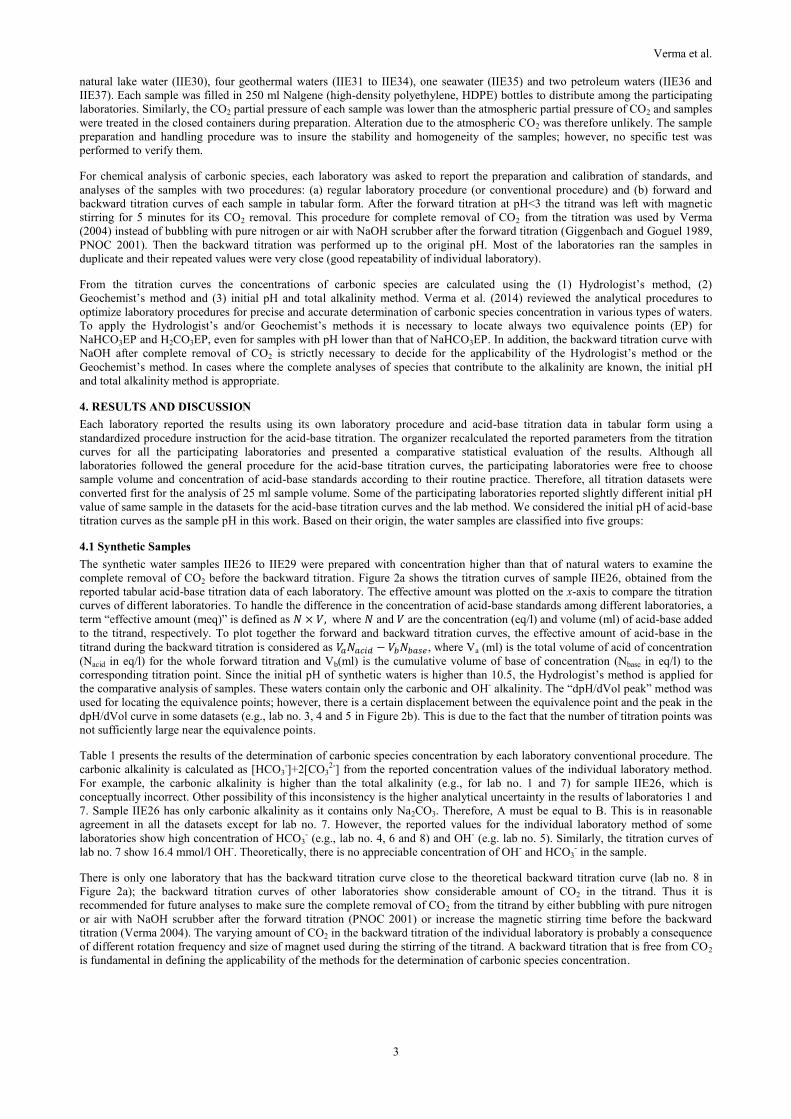
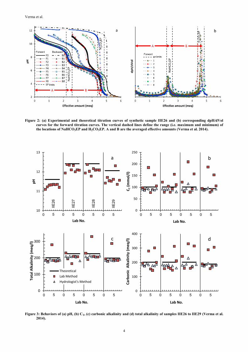
The synthetic water samples IIE26 to IIE29 were prepared with concentration higher than that of natural waters to examine the

complete removal of CO2 before the backward titration. Figure 2a shows the titration curves of sample IIE26, obtained from the

reported tabular acid-base titration data of each laboratory. The effective amount was plotted on the x-axis to compare the titration

curves of different laboratories. To handle the difference in the concentration of acid-base standards among different laboratories, a

term “effective amount (meq)” is defined as where and are the concentration (eq/l) and volume (ml) of acid-base added

to the titrand, respectively. To plot together the forward and backward titration curves, the effective amount of acid-base in the

titrand during the backward titration is considered as , where Va (ml) is the total volume of acid of concentration

(Nacid in eq/l) for the whole forward titration and Vb(ml) is the cumulative volume of base of concentration (Nbase in eq/l) to the

corresponding titration point. Since the initial pH of synthetic waters is higher than 10.5, the Hydrologist’s method is applied for

the comparative analysis of samples. These waters contain only the carbonic and OH- alkalinity. The “dpH/dVol peak” method was

used for locating the equivalence points; however, there is a certain displacement between the equivalence point and the peak in the

dpH/dVol curve in some datasets (e.g., lab no. 3, 4 and 5 in Figure 2b). This is due to the fact that the number of titration points was

not sufficiently large near the equivalence points.

Table 1 presents the results of the determination of carbonic species concentration by each laboratory conventional procedure. The

carbonic alkalinity is calculated as [HCO3-]+2[CO3

2-] from the reported concentration values of the individual laboratory method.

For example, the carbonic alkalinity is higher than the total alkalinity (e.g., for lab no. 1 and 7) for sample IIE26, which is

conceptually incorrect. Other possibility of this inconsistency is the higher analytical uncertainty in the results of laboratories 1 and

7. Sample IIE26 has only carbonic alkalinity as it contains only Na2CO3. Therefore, A must be equal to B. This is in reasonable

agreement in all the datasets except for lab no. 7. However, the reported values for the individual laboratory method of some

laboratories show high concentration of HCO3- (e.g., lab no. 4, 6 and 8) and OH- (e.g. lab no. 5). Similarly, the titration curves of

lab no. 7 show 16.4 mmol/l OH-. Theoretically, there is no appreciable concentration of OH- and HCO3- in the sample.

There is only one laboratory that has the backward titration curve close to the theoretical backward titration curve (lab no. 8 in

Figure 2a); the backward titration curves of other laboratories show considerable amount of CO2 in the titrand. Thus it is

recommended for future analyses to make sure the complete removal of CO2 from the titrand by either bubbling with pure nitrogen

or air with NaOH scrubber after the forward titration (PNOC 2001) or increase the magnetic stirring time before the backward

titration (Verma 2004). The varying amount of CO2 in the backward titration of the individual laboratory is probably a consequence

of different rotation frequency and size of magnet used during the stirring of the titrand. A backward titration that is free from CO2

is fundamental in defining the applicability of the methods for the determination of carbonic species concentration.

Verma et al.

4

Figure 2: (a) Experimental and theoretical titration curves of synthetic sample IIE26 and (b) corresponding dpH/dVol

curves for the forward titration curves. The vertical dashed lines define the range (i.e. maximum and minimum) of

the locations of NaHCO3EP and H2CO3EP. A and B are the averaged effective amounts (Verma et al. 2014).

Figure 3: Behaviors of (a) pH, (b) CT, (c) carbonic alkalinity and (d) total alkalinity of samples IIE26 to IIE29 (Verma et al.

2014).

10

11

12

13

pH

Lab No.

0

50

100

150

200

250

CT

(mm

ol/

l)

Lab No.

0

100

200

300

Tota

l Alk

alin

ity

(me

q/l

)

Lab No.

Theoretical

Lab Method

Hydrologist's Method

0

100

200

300

400

Car

bo

nic

Alk

alin

ity

(me

q/l

)

Lab No.

a

0 5 0 5 0 5 0 5

IIE

26

IIE

29

IIE

28

IIE

27

0 5 0 5 0 5 0 5

0 5 0 5 0 5 0 5 0 5 0 5 0 5 0 5

b

c d

Verma et al.

5

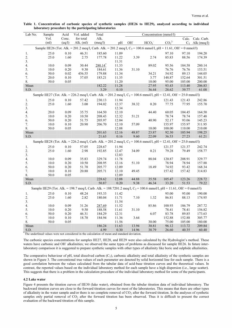
Table 1. Concentration of carbonic species of synthetic samples (IIE26 to IIE29), analyzed according to individual

laboratory procedure by the participating laboratories

Lab No. Sample

Vol.

(ml)

Acid

Conc.

(eq/l)

Vol. added

for total

Alk. (ml)

Total

Alk.

(meq/l) pH

Concentration (mmol/l)

Calc. Carb.

Alk (meq/l) OH- HCO3- CO3

2- Calc.

CT

Sample IIE26 (Tot. Alk. = 201.2 meq/l, Carb. Alk. = 201.2 meq/l, CT = 100.6 mmol/l, pH = 11.61, OH- = 0 mmol/l)

1. 25.0 0.10 46.31 185.60 11.09 97.10 97.10 194.20

2. 25.0 1.60 2.75 177.78 11.22 3.39 2.74 85.83 88.56 174.39

3. 11.31

4. 10.0 0.09 30.44 280.14* 11.33 89.02 95.56 184.58 280.14

5. 10.0 0.20 9.30 184.61 11.36 31.10 76.76 76.76 153.51

6. 50.0 0.02 456.55 179.88 11.34 34.21 54.92 89.13 144.05

7. 20.0 0.10 37.05 183.21 11.35 3.77 148.87 152.64 301.51

8. 50.0 0.05 11.20 10.00 95.00 105.00 200.00

Mean 182.22 11.28 27.95 93.43 113.40 206.83

S.D. 3.29 0.10 36.44 28.62 39.77 61.08

Sample IIE27 (Tot. Alk. = 226.2 meq/l, Carb. Alk. = 201.2 meq/l, CT = 100.6 mmol/l, pH = 12.41, OH- = 25.0 mmol/l)

1. 25.0 0.10 57.42 230.13 11.94 121.43 121.43 242.86

2. 25.0 1.60 3.00 194.02 12.37 38.32 0.20 77.75 77.95 155.70

3. 12.34

4. 20.0 0.09 35.75 164.50 12.10 44.40 60.05 104.45 164.50

5. 10.0 0.20 10.50 208.43 12.32 51.21 78.74 78.74 157.48

6. 50.0 0.20 51.75 205.97 12.04 40.90 52.17 93.06 145.23

7. 10.0 0.10 20.90 206.70 12.10 57.09 155.97 155.97 311.95

8. 50.0 0.05 12.08 10.00 100.00 110.00 210.00

Mean 201.63 12.16 48.87 23.87 92.30 105.94 198.25

S.D. 21.63 0.16 9.60 22.09 36.53 27.23 61.21

Sample IIE28 (Tot. Alk. = 226.2 meq/l, Carb. Alk. = 201.2 meq/l, CT = 100.6 mmol/l, pH = 12.41, OH- = 25.0 mmol/l)

1. 25.0 0.10 57.05 228.67 11.94 121.37 121.37 242.74

2. 25.0 1.60 2.98 192.85 12.47 34.09 0.21 79.28 79.49 158.77

3. 12.03

4. 10.0 0.09 35.83 329.74 11.78 88.04 120.87 208.91 329.77

5. 10.0 0.20 10.50 208.95 12.16 51.10 78.94 78.94 157.88

6. 50.0 0.20 51.70 205.77 12.09 18.49 74.92 93.42 168.34

7. 10.0 0.10 20.80 205.71 12.10 49.45 157.42 157.42 314.83

8. 50.0 0.05 12.09

Mean 228.62 12.08 44.88 35.58 105.47 123.26 228.72

S.D. 50.87 0.20 9.38 46.34 33.20 51.53 79.22

Sample IIE29 (Tot. Alk. = 198.7 meq/l, Carb. Alk. = 188.7201.2 meq/l, CT = 100.6 mmol/l, pH = 11.61, OH- = 0 mmol/l)

1. 25.0 0.10 48.24 193.33 11.42 95.00 95.00 190.00

2. 25.0 1.60 2.82 180.04 11.71 7.10 1.32 86.81 88.13 174.95

3. 11.54

4. 10.0 0.09 31.26 287.69 11.52 85.86 100.93 186.79 287.72

5. 10.0 0.20 9.50 188.58 11.61 31.10 78.41 78.41 156.82

6. 50.0 0.20 46.31 184.29 12.31 6.07 83.78 89.85 173.63

7. 10.0 0.10 18.70 184.94 11.36 3.64 152.88 152.88 305.77

8. 50.0 0.05 11.56 30.00 75.00 105.00 180.00

Mean 186.24 11.63 13.94 30.81 96.12 113.72 209.84

S.D. 4.99 0.30 14.96 38.79 26.60 40.35 60.40 * The underlined values were not considered in the calculation of mean and standard deviation.

The carbonic species concentrations for samples IIE27, IIE28, and IIE29 were also calculated by the Hydrologist’s method. These

waters have carbonic and OH- alkalinities; we observed the same types of problems as discussed for sample IIE26. In future inter-

laboratory comparison it is suggested to prepare synthetic samples with other types of alkalinity like boric and sulphide alkalinities.

The comparative behaviour of pH, total dissolved carbon (CT), carbonic alkalinity and total alkalinity of the synthetic samples are

shown in Figure 3. The conventional true values of each parameter are denoted by solid horizontal line for each sample. There is a

good correlation between the values calculated from the tabular data of acid-base titration curves and the theoretical values. In

contrast, the reported values based on the individual laboratory method for each sample have a high dispersion (i.e., large scatter).

This suggests that there is a problem in the calculation procedure of the individual laboratory method for some of the participants.

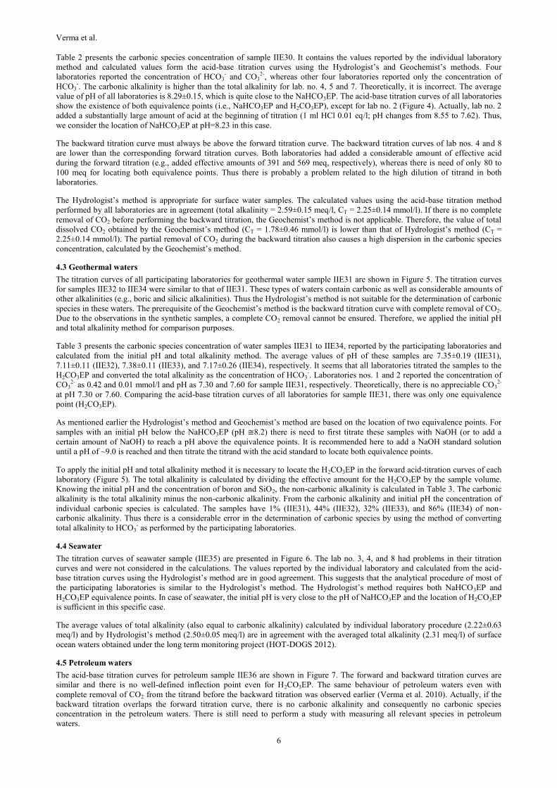
4.2 Lake water

Figure 4 presents the titration curves of IIE30 (lake water), obtained from the tabular titration data of individual laboratory. The

backward titration curves are close to the forward titration curves for most of the laboratories. This means that there are other types

of alkalinity in the water sample and/or there is no complete removal of CO2 after the forward titration. In the analyses of synthetic

samples only partial removal of CO2 after the forward titration has been observed. Thus it is difficult to present the correct

evaluation of the backward titration of this sample.

Verma et al.

6

Table 2 presents the carbonic species concentration of sample IIE30. It contains the values reported by the individual laboratory

method and calculated values form the acid-base titration curves using the Hydrologist’s and Geochemist’s methods. Four

laboratories reported the concentration of HCO3- and CO3

2-, whereas other four laboratories reported only the concentration of

HCO3-. The carbonic alkalinity is higher than the total alkalinity for lab. no. 4, 5 and 7. Theoretically, it is incorrect. The average

value of pH of all laboratories is 8.29±0.15, which is quite close to the NaHCO3EP. The acid-base titration curves of all laboratories

show the existence of both equivalence points (i.e., NaHCO3EP and H2CO3EP), except for lab no. 2 (Figure 4). Actually, lab no. 2

added a substantially large amount of acid at the beginning of titration (1 ml HCl 0.01 eq/l; pH changes from 8.55 to 7.62). Thus,

we consider the location of NaHCO3EP at pH=8.23 in this case.

The backward titration curve must always be above the forward titration curve. The backward titration curves of lab nos. 4 and 8

are lower than the corresponding forward titration curves. Both laboratories had added a considerable amount of effective acid

during the forward titration (e.g., added effective amounts of 391 and 569 meq, respectively), whereas there is need of only 80 to

100 meq for locating both equivalence points. Thus there is probably a problem related to the high dilution of titrand in both

laboratories.

The Hydrologist’s method is appropriate for surface water samples. The calculated values using the acid-base titration method

performed by all laboratories are in agreement (total alkalinity = 2.59±0.15 meq/l, CT = 2.25±0.14 mmol/l). If there is no complete

removal of CO2 before performing the backward titration, the Geochemist’s method is not applicable. Therefore, the value of total

dissolved CO2 obtained by the Geochemist’s method (CT = 1.78±0.46 mmol/l) is lower than that of Hydrologist’s method (CT =

2.25±0.14 mmol/l). The partial removal of CO2 during the backward titration also causes a high dispersion in the carbonic species

concentration, calculated by the Geochemist’s method.

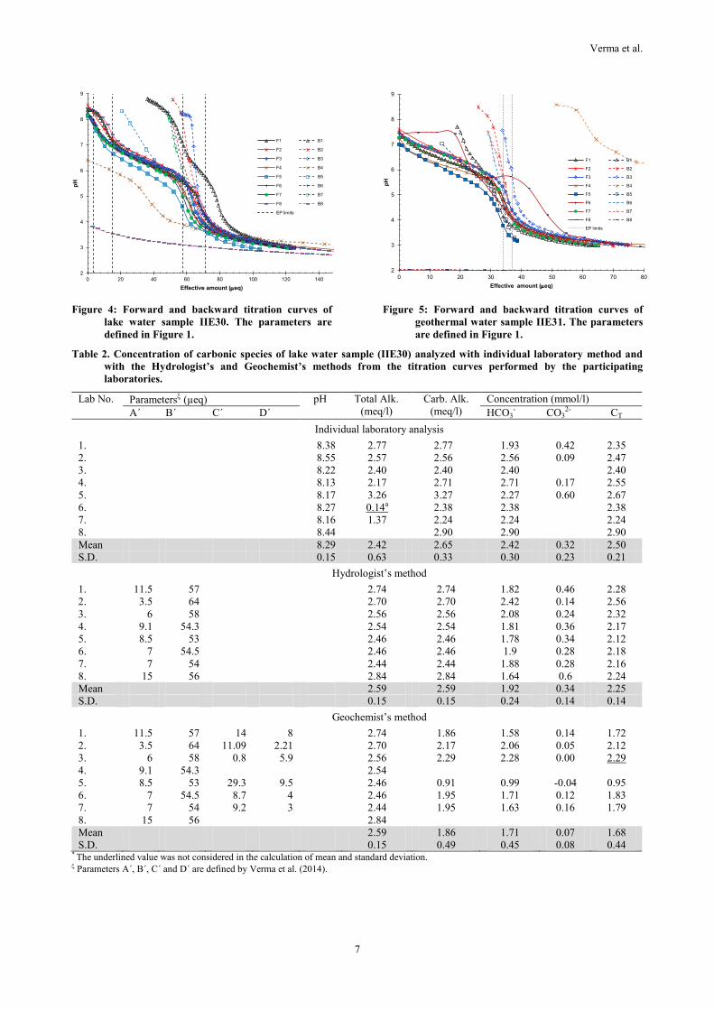
4.3 Geothermal waters

The titration curves of all participating laboratories for geothermal water sample IIE31 are shown in Figure 5. The titration curves

for samples IIE32 to IIE34 were similar to that of IIE31. These types of waters contain carbonic as well as considerable amounts of

other alkalinities (e.g., boric and silicic alkalinities). Thus the Hydrologist’s method is not suitable for the determination of carbonic

species in these waters. The prerequisite of the Geochemist’s method is the backward titration curve with complete removal of CO2.

Due to the observations in the synthetic samples, a complete CO2 removal cannot be ensured. Therefore, we applied the initial pH

and total alkalinity method for comparison purposes.

Table 3 presents the carbonic species concentration of water samples IIE31 to IIE34, reported by the participating laboratories and

calculated from the initial pH and total alkalinity method. The average values of pH of these samples are 7.35±0.19 (IIE31),

7.11±0.11 (IIE32), 7.38±0.11 (IIE33), and 7.17±0.26 (IIE34), respectively. It seems that all laboratories titrated the samples to the

H2CO3EP and converted the total alkalinity as the concentration of HCO3-. Laboratories nos. 1 and 2 reported the concentration of

CO32- as 0.42 and 0.01 mmol/l and pH as 7.30 and 7.60 for sample IIE31, respectively. Theoretically, there is no appreciable CO3

2-

at pH 7.30 or 7.60. Comparing the acid-base titration curves of all laboratories for sample IIE31, there was only one equivalence

point (H2CO3EP).

As mentioned earlier the Hydrologist’s method and Geochemist’s method are based on the location of two equivalence points. For

samples with an initial pH below the NaHCO3EP (pH 8.2) there is need to first titrate these samples with NaOH (or to add a

certain amount of NaOH) to reach a pH above the equivalence points. It is recommended here to add a NaOH standard solution

until a pH of ~9.0 is reached and then titrate the titrand with the acid standard to locate both equivalence points.

To apply the initial pH and total alkalinity method it is necessary to locate the H2CO3EP in the forward acid-titration curves of each

laboratory (Figure 5). The total alkalinity is calculated by dividing the effective amount for the H2CO3EP by the sample volume.

Knowing the initial pH and the concentration of boron and SiO2, the non-carbonic alkalinity is calculated in Table 3. The carbonic

alkalinity is the total alkalinity minus the non-carbonic alkalinity. From the carbonic alkalinity and initial pH the concentration of

individual carbonic species is calculated. The samples have 1% (IIE31), 44% (IIE32), 32% (IIE33), and 86% (IIE34) of non-

carbonic alkalinity. Thus there is a considerable error in the determination of carbonic species by using the method of converting

total alkalinity to HCO3- as performed by the participating laboratories.

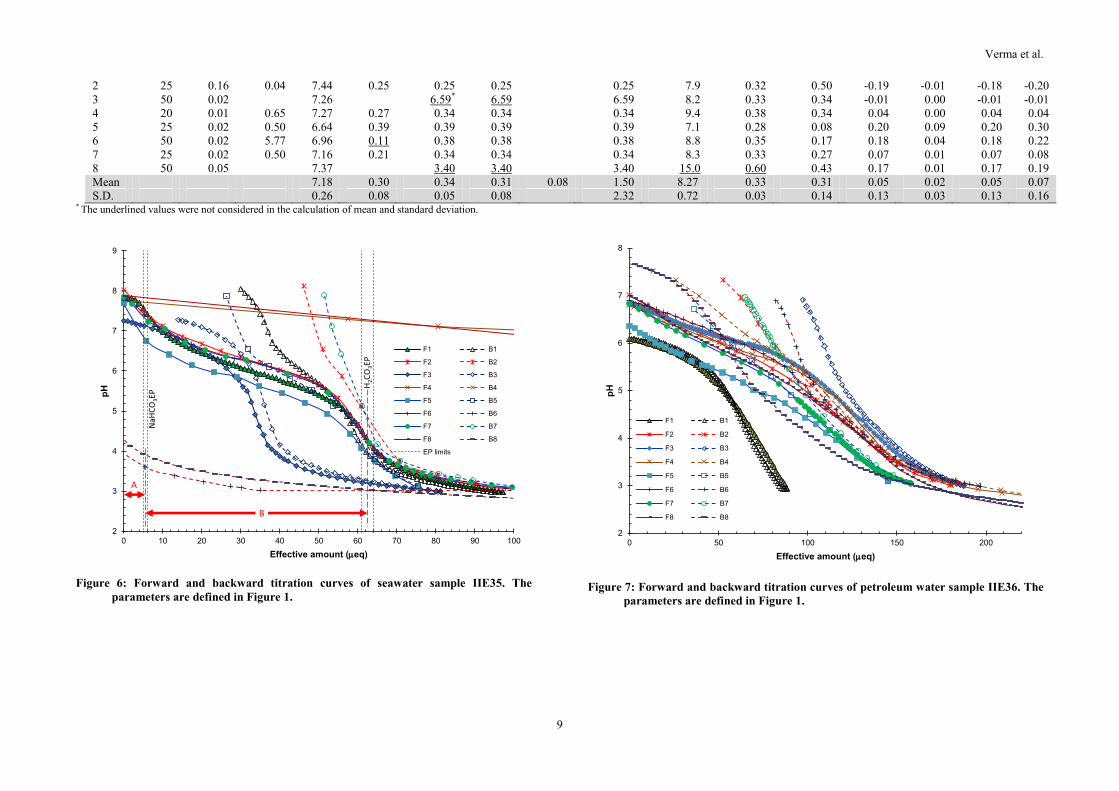
4.4 Seawater

The titration curves of seawater sample (IIE35) are presented in Figure 6. The lab no. 3, 4, and 8 had problems in their titration

curves and were not considered in the calculations. The values reported by the individual laboratory and calculated from the acid-

base titration curves using the Hydrologist’s method are in good agreement. This suggests that the analytical procedure of most of

the participating laboratories is similar to the Hydrologist’s method. The Hydrologist’s method requires both NaHCO3EP and

H2CO3EP equivalence points. In case of seawater, the initial pH is very close to the pH of NaHCO3EP and the location of H2CO3EP

is sufficient in this specific case.

The average values of total alkalinity (also equal to carbonic alkalinity) calculated by individual laboratory procedure (2.22±0.63

meq/l) and by Hydrologist’s method (2.50±0.05 meq/l) are in agreement with the averaged total alkalinity (2.31 meq/l) of surface

ocean waters obtained under the long term monitoring project (HOT-DOGS 2012).

4.5 Petroleum waters

The acid-base titration curves for petroleum sample IIE36 are shown in Figure 7. The forward and backward titration curves are

similar and there is no well-defined inflection point even for H2CO3EP. The same behaviour of petroleum waters even with

complete removal of CO2 from the titrand before the backward titration was observed earlier (Verma et al. 2010). Actually, if the

backward titration overlaps the forward titration curve, there is no carbonic alkalinity and consequently no carbonic species

concentration in the petroleum waters. There is still need to perform a study with measuring all relevant species in petroleum

waters.

Verma et al.

7

Figure 4: Forward and backward titration curves of

lake water sample IIE30. The parameters are

defined in Figure 1.

Figure 5: Forward and backward titration curves of

geothermal water sample IIE31. The parameters

are defined in Figure 1.

Table 2. Concentration of carbonic species of lake water sample (IIE30) analyzed with individual laboratory method and

with the Hydrologist’s and Geochemist’s methods from the titration curves performed by the participating

laboratories.

Lab No. Parameters (µeq) pH Total Alk.

(meq/l)

Carb. Alk.

(meq/l)

Concentration (mmol/l)

A´ B´ C´ D´ HCO3- CO3

2- CT

Individual laboratory analysis

1. 8.38 2.77 2.77 1.93 0.42 2.35

2. 8.55 2.57 2.56 2.56 0.09 2.47

3. 8.22 2.40 2.40 2.40 2.40

4. 8.13 2.17 2.71 2.71 0.17 2.55

5. 8.17 3.26 3.27 2.27 0.60 2.67

6. 8.27 0.14a 2.38 2.38 2.38

7. 8.16 1.37 2.24 2.24 2.24

8. 8.44 2.90 2.90 2.90

Mean 8.29 2.42 2.65 2.42 0.32 2.50

S.D. 0.15 0.63 0.33 0.30 0.23 0.21

Hydrologist’s method

1. 11.5 57 2.74 2.74 1.82 0.46 2.28

2. 3.5 64 2.70 2.70 2.42 0.14 2.56

3. 6 58 2.56 2.56 2.08 0.24 2.32

4. 9.1 54.3 2.54 2.54 1.81 0.36 2.17

5. 8.5 53 2.46 2.46 1.78 0.34 2.12

6. 7 54.5 2.46 2.46 1.9 0.28 2.18

7. 7 54 2.44 2.44 1.88 0.28 2.16

8. 15 56 2.84 2.84 1.64 0.6 2.24

Mean 2.59 2.59 1.92 0.34 2.25

S.D. 0.15 0.15 0.24 0.14 0.14

Geochemist’s method

1. 11.5 57 14 8 2.74 1.86 1.58 0.14 1.72

2. 3.5 64 11.09 2.21 2.70 2.17 2.06 0.05 2.12

3. 6 58 0.8 5.9 2.56 2.29 2.28 0.00 2.29

4. 9.1 54.3 2.54

5. 8.5 53 29.3 9.5 2.46 0.91 0.99 -0.04 0.95

6. 7 54.5 8.7 4 2.46 1.95 1.71 0.12 1.83

7. 7 54 9.2 3 2.44 1.95 1.63 0.16 1.79

8. 15 56 2.84

Mean 2.59 1.86 1.71 0.07 1.68

S.D. 0.15 0.49 0.45 0.08 0.44 * The underlined value was not considered in the calculation of mean and standard deviation.

Parameters A´, B´, C´ and D´ are defined by Verma et al. (2014).

2

3

4

5

6

7

8

9

0 20 40 60 80 100 120 140

pH

Effective amount (eq)

F1 B1

F2 B2

F3 B3

F4 B4

F5 B5

F6 B6

F7 B7

F8 B8

EP limits

2

3

4

5

6

7

8

9

0 10 20 30 40 50 60 70 80

pH

Effective amount (eq)

F1 B1

F2 B2

F3 B3

F4 B4

F5 B5

F6 B6

F7 B7

F8 B8

EP limits

Verma et al.

8

Table 3. Concentration of carbonic species of geothermal water samples (IIE31 to IIE34) analyzed with individual laboratory method, and with the initial pH and total alkalinity method

using the titration curves performed by the participating laboratories.

Lab

No.

Laboratory method Initial pH and total alkalinity method using titration curves of individual laboratory

Sample

Vol (ml)

Acid

(eq/l)

Acid

Vol

(ml)

pH Alkalinity

(meq/l)

Concentration

(mmol/l)

Effective

amount

(µeq)

Alkalinity

(meq/l)

Concentration

(mmol/l)

Total Alk Car. Alk. HCO3- CO3

2- CT Total Alk. Non Carb.

Alk.

Carb.

Alk.

H2CO3 HCO3- CT

Sample IIE31 (SiO2= 2.16 mmol/l, B=0.31 mmol/l)

1 25 0.10 0.69 7.30 2.77 1.40 1.16 0.12 1.28 34.8 1.40 1.01E-2 1.38 0.14 1.38 1.52

2 25 0.16 0.20 7.60 1.27 1.27 1.26 0.01 1.27 35.5 1.42 2.01E-2 1.40 0.07 1.39 1.47

3 50 0.02 7.45 1.42 1.42 1.42 35.9 1.44 1.42E-2 1.42 0.10 1.42 1.52

4 20 0.01 2.76 7.23 1.44 1.44 1.44 1.44 35.2 1.41 8.62E-3 1.40 0.16 1.40 1.56

5 10 0.02 0.80 7.00 1.51 1.55 1.55 1.55 34.0 1.36 5.09E-3 1.35 0.27 1.35 1.62

6 50 0.02 4.80 7.51 1.89 1.55 1.55 1.55 37.0 1.48 1.64E-2 1.46 0.09 1.46 1.55

7 25 0.02 2.00 7.28 1.58 1.30 1.30 1.30 37.0 1.48 9.67E-3 1.47 0.15 1.47 1.62

8 50 0.05 7.41 2.20 2.20 2.20

Mean 7.35 1.74 1.42 1.38 0.07 1.40 35.63 1.43 0.01 1.41 0.14 1.41 1.55

S.D. 0.19 0.54 0.11 0.145 0.12 1.11 0.04 0.01 0.04 0.07 0.04 0.06

Sample IIE32 (SiO2= 15.76 mmol/l, B=51.64 mmol/l)

1 25 0.10 0.25 7.15 1.01 1.00 1.00 1.00 24.1 0.96 0.46 0.50 0.07 0.50 0.58

2 25 0.16 0.13 7.30 0.84 0.83 0.83 0.83 23.2 0.93 0.65 0.28 0.03 0.28 0.31

3 50 0.02 7.16 24.4 0.98 0.47 0.50 0.07 0.50 0.57

4 20 0.01 1.91 7.03 0.79 0.99 0.99 0.99 25.0 1.00 0.35 0.65 0.12 0.65 0.77

5 25 0.02 1.45 6.95 1.10 1.11 1.11 1.11 28.0 1.12 0.29 0.83 0.19 0.83 1.01

6 50 0.02 18.68 7.03 0.37 0.88 0.88 0.88 24.1 0.96 0.35 0.61 0.11 0.61 0.73

7 25 0.02 1.45 7.08 0.57 0.93 0.93 0.93 23.0 0.92 0.39 0.53 0.09 0.53 0.62

8 50 0.05 7.16 1.80 1.80 1.80 24.0 0.96 0.47 0.49 0.07 0.49 0.56

Mean 7.11 0.78 0.96 0.96 0.96 23.97 0.96 0.43 0.55 0.09 0.55 0.64

S.D. 0.11 0.27 0.10 0.10 0.10 0.68 0.03 0.11 0.16 0.05 0.16 0.20

Sample IIE33 (SiO2= 17.46 mmol/l, B=33.76 mmol/l)

1 25 0.10 0.29 7.38 1.16 1.16 1.16 1.12 28.0 1.12 0.53 0.59 0.05 0.58 0.63

2 25 0.16 0.13 7.55 0.87 0.87 0.87 1.05 26.3 1.05 0.78 0.27 0.01 0.27 0.28

3 50 0.02 7.46 1.14 28.5 1.14 0.64 0.50 0.03 0.50 0.53

4 20 0.01 2.23 7.23 0.93 1.16 1.16 1.16 29.0 1.16 0.38 0.78 0.09 0.78 0.87

5 10 0.02 0.70 7.23 1.32 1.33 1.33 1.08 27.0 1.08 0.38 0.70 0.08 0.70 0.78

6 50 0.02 18.72 7.43 0.37 0.57 0.57 1.07 26.7 1.07 0.60 0.47 0.03 0.47 0.50

7 25 0.02 1.60 7.33 0.63 1.03 1.03 1.09 27.2 1.09 0.48 0.61 0.06 0.61 0.67

8 50 0.05 7.41 1.00 1.00 1.21 30.3 1.21 0.57 0.64 0.05 0.64 0.69

Mean 7.38 0.98 1.09 1.09 1.02 27.88 1.12 0.55 0.57 0.05 0.57 0.62

S.D. 0.11 0.27 0.16 0.16 0.25 1.34 0.05 0.14 0.16 0.03 0.16 0.18

Sample IIE34 (SiO2= 15.54 mmol/l, B=27.38 mmol/l)

1 25 0.10 0.09 7.30 0.36 0.35 0.19 0.08 0.27 8.2 0.33 0.36 -0.04 0.00 -0.04 -0.04

Verma et al.

9

2 25 0.16 0.04 7.44 0.25 0.25 0.25 0.25 7.9 0.32 0.50 -0.19 -0.01 -0.18 -0.20

3 50 0.02 7.26 6.59* 6.59 6.59 8.2 0.33 0.34 -0.01 0.00 -0.01 -0.01

4 20 0.01 0.65 7.27 0.27 0.34 0.34 0.34 9.4 0.38 0.34 0.04 0.00 0.04 0.04

5 25 0.02 0.50 6.64 0.39 0.39 0.39 0.39 7.1 0.28 0.08 0.20 0.09 0.20 0.30

6 50 0.02 5.77 6.96 0.11 0.38 0.38 0.38 8.8 0.35 0.17 0.18 0.04 0.18 0.22

7 25 0.02 0.50 7.16 0.21 0.34 0.34 0.34 8.3 0.33 0.27 0.07 0.01 0.07 0.08

8 50 0.05 7.37 3.40 3.40 3.40 15.0 0.60 0.43 0.17 0.01 0.17 0.19

Mean 7.18 0.30 0.34 0.31 0.08 1.50 8.27 0.33 0.31 0.05 0.02 0.05 0.07

S.D. 0.26 0.08 0.05 0.08 2.32 0.72 0.03 0.14 0.13 0.03 0.13 0.16 * The underlined values were not considered in the calculation of mean and standard deviation.

Figure 6: Forward and backward titration curves of seawater sample IIE35. The

parameters are defined in Figure 1.

Figure 7: Forward and backward titration curves of petroleum water sample IIE36. The

parameters are defined in Figure 1.

2

3

4

5

6

7

8

9

0 10 20 30 40 50 60 70 80 90 100

pH

Effective amount (eq)

F1 B1

F2 B2

F3 B3

F4 B4

F5 B5

F6 B6

F7 B7

F8 B8

EP limits

NaH

CO

3EP

H2C

O3E

P

A

B

2

3

4

5

6

7

8

0 50 100 150 200

pH

Effective amount (eq)

F1 B1

F2 B2

F3 B3

F4 B4

F5 B5

F6 B6

F7 B7

F8 B8

Verma et al.

10

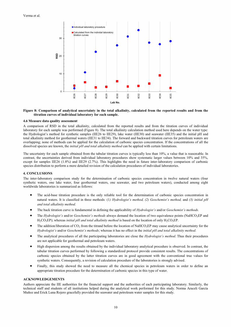
Figure 8: Comparison of analytical uncertainty in the total alkalinity, calculated from the reported results and from the

titration curves of individual laboratory for each sample.

4.6 Measure data quality assessment

A comparison of RSD in the total alkalinity, calculated from the reported results and from the titration curves of individual

laboratory for each sample was performed (Figure 8). The total alkalinity calculation method used here depends on the water type:

the Hydrologist’s method for synthetic samples (IIE26 to IIE29), lake water (IIE30) and seawater (IIE35) and the initial pH and

total alkalinity method for geothermal waters (IIE31 to IIE34). The forward and backward titration curves for petroleum waters are

overlapping; none of methods can be applied for the calculation of carbonic species concentration. If the concentrations of all the

dissolved species are known, the initial pH and total alkalinity method can be applied with certain limitations.

The uncertainty for each sample obtained from the tabular titration curves is typically less than 10%, a value that is reasonable. In

contrast, the uncertainties derived from individual laboratory procedures show systematic larger values between 10% and 35%,

except for samples IIE26 (1.8%) and IIE29 (2.7%). This highlights the need in future inter-laboratory comparison of carbonic

species distribution to perform a more detailed revision of the calculation procedures of individual laboratories.

4. CONCLUSIONS

The inter-laboratory comparison study for the determination of carbonic species concentration in twelve natural waters (four

synthetic waters, one lake water, four geothermal waters, one seawater, and two petroleum waters), conducted among eight

worldwide laboratories is summarized as follows:

The acid-base titration procedure is the only reliable tool for the determination of carbonic species concentration in

natural waters. It is classified in three methods: (1) Hydrologist’s method, (2) Geochemist’s method, and (3) initial pH

and total alkalinity method.

The back titration curve is fundamental in defining the applicability of Hydrologist’s and/or Geochemist’s methods.

The Hydrologist’s and/or Geochemist’s methods always demand the location of two equivalence points (NaHCO3EP and

H2CO3EP); whereas initial pH and total alkalinity method is based on the location of only H2CO3EP.

The addition/liberation of CO2 from the titrand before the location of NaHCO3EP may cause analytical uncertainty for the

Hydrologist’s and/or Geochemist’s methods; whereas it has no effect in the initial pH and total alkalinity method.

The analytical procedures of all the participating laboratories are close the Hydrologist’s method. Thus their procedures

are not applicable for geothermal and petroleum waters.

High dispersion among the results obtained by the individual laboratory analytical procedure is observed. In contrast, the

tabular titration curves performed by following a standardized protocol provide consistent results. The concentrations of

carbonic species obtained by the latter titration curves are in good agreement with the conventional true values for

synthetic waters. Consequently, a revision of calculation procedure of the laboratories is strongly advised.

Finally, this study showed the need to measure all the chemical species in petroleum waters in order to define an

appropriate titration procedure for the determination of carbonic species in this type of water.

ACKNOWLEDGEMENTS

Authors appreciate the IIE authorities for the financial support and the authorities of each participating laboratory. Similarly, the

technical staff and students of all institutions helped during the analytical work performed for this study. Norma Araceli García

Muñoz and Erick Luna Rojero gracefully provided the seawater and petroleum water samples for this study.

0

10

20

30

40

RS

D

Lab No.

Individual laboratory procedure

Calculated from the individal laboratorytitration curves

IIE2

6

IIE2

7

IIE2

8

IIE2

9

IIE3

0

IIE3

1

IIE3

2

IIE3

3

IIE3

4

IIE3

5

Verma et al.

11

REFERENCES

Alvis-Isidro, R., Urbino, G.A., and Gerardo-Abaya, J.: 1999 interlaboratory comparison of geothermal water chemistry under IAEA

regional project RAS/8/075, Report, IAEA, Vienna (1999).

Alvis-Isidro, R., Urbino, G.A., and Pang, Z.: Results of the 2000 IAEA interlaboratory comparison of geothermal water chemistry,

Report, IAEA, Vienna (2000).

Alvis-Isidro, R., Urbino, G.A., and Pang, Z.: 2001 interlaboratory comparison of geothermal water chemistry, Report, IAEA,

Vienna (2002).

Ellis, A.J.: The IAGC interlaboratory water analysis comparison programme, Geochimica et Cosmochimica Acta, 40, (1976) 1359-

1374.

Gerardo-Abaya, J., Schueszler, C. and Gröening, M.: Results of the interlaboratory comparison for water chemistry in natural

geothermal samples under RAS/8/075., Report, Vienna, IAEA (1998).

Giggenbach, W.F. and Goguel, R.L.: Collection and analysis of geothermal water and volcanic water and gas discharges, 4th

Edition. Department of Scientific and Industrial Researsh, Petone, New Zealand (1989).

Giggenbach, W.F., Goguel, R.L. and Humphries, W.A. IAEA interlaboratory comparative geothermal water analysis program.

Geothermal Investigations with Isotope and Geothermal Techniques in Latin America, IAEA-TECDOC-641, Vienna, (1992)

439-456.

HOT-DOGS: Hawaii Ocean Time-series Data Organization & Graphical System. http://hahana.soest.hawaii.edu/hot/hot-dogs/

(Accessed on October 1, 2012).

NASA: Carbon cycle, http://science.nasa.gov/earth-science/oceanography/ocean-earth-system/ocean-carbon-cycle/ (Accessed in

October 1, 2012).

PNOC (Philippine National Oil Company): Bicarbonate, carbonate and total carbon dioxide. Laboratory Procedure Manual,

Philippines (2001).

Stumm, W. and Morgan, J.J.: Aquatic chemistry: Chemical equilibria and rates in natural waters, John Wiley & Sons, Inc., New

York (1996).

Torres-Alvarado, I.S., Verma, M.P., Opondo, K., Nieva, D., Haklidir, F.T., Santoyo, E., Barragán, R.M. and Arellano, V.:

Estimates of geothermal reservoir fluid characteristics:GeoSys.Chem and WATCH, Revista Mexicana de Ciencias

Geológicas, 29, (2012) 713–724.

Urbino, G.A., and Pang, Z.: 2003 interlaboratory comparison of geothermal water chemistry, Report, PNOC, Philippines (2004).

van Geldern, R., Verma, M.P., Carvalho, C.M., Grassa, F., Delgado-Huertas, A., Monvoisin, G. and Barth, J.A.C.: Stable carbon

isotope analysis of dissolved inorganic carbon (DIC) and dissolved organic carbon (DOC) in natural waters – Results from a

worldwide proficiency test, Rapid Communications in Mass Spectrometry, 27, (2013) 2099–2107.

Verma, M.P.: A revised analytical method for HCO3- and CO3

2- determinations in geothermal waters: an assessment of IAGC and

IAEA interlaboratory comparisons, Geostandards and Geoanalytical Research, 28, (2004) 391–409

Verma M.P.: Revised analytical methods for the determination of carbonic species in rain, ground and geothermal waters,

Proceedings, World Geothermal Congress, Antalya, Turkey (2005).

Verma, M.P.: IAGC and IAEA Interlaboratory Comparisons of Geothermal Water Chemistry: the propagation of errors in the

reservoir pH calculation, Geostandards and Geoanalytical Research, 32, (2008) 317-330.

Verma, M.P.: IAEA Inter-laboratory Comparisons of Geothermal Water Chemistry: Critiques on Analytical Uncertainty and

Accuracy, and Geothermal Reservoir Modeling, Journal of Iberian Geology, 39, (2013)57-72.

Verma M.P.: Compositional Statistical Analysis of Inter-laboratory Comparison of Geothermal Water Chemistry. Proceedings,

Geostatistical and Geospatial approaches for the characterization of natural resources in the environment: challenges,

processes and strategies, New Delhi (2014).

Verma, M.P., Birkle, P. and Sánchez, D. Theoretical and Analytical Aspects of Carbonic Species Determination in Rain, Ground,

Geothermal and Petroleum Waters, Proceedings, World Geothermal Congress, Bali, Indonesia (2010).

Verma, M.P., Izquierdo, G., Urbino, G.A., Gangloff, S., Garcia, R., Aparicio, A., Conte, T., Armienta, M.A., Sanchez, M., Gabriel,

J.R.P., Fajanela, I.D., Renderos, R., Acha, C.B.A., Prasetio, R., Grajales, I.C, Delgado, L.R., Opondo, K., Esparza, R.Z.,

Panama, L.A., Salazar, R.T., Lim, P.G., Javino, F.: Inter-laboratory comparison of SiO2 analysis for geothermal water

chemistry, Geothermics, 44, (2012)32-42.

Verma, M.P., Izquierdo, G., Sangloff, S., Reyes-Delgado, L., Armienta, M.A., Sanchez, M., Garcia, R. and Turdiaman, D.:

Proficiency testing statistics on Si-determinations in geothermal waters, in preparation (2015).

Verma, M.P., Portugal, E., Gangloff, S., Armienta, Ma.A., Chandrasekharam, D., Sanchez, M., Renderos, R.E., Junaco, M., van

Geldern, R.: Determination of carbonic species concentration in natural waters - Results from a worldwide proficiency test,

Geostandards and Geoanalytical Research (2014). Article first published online: 26 AUG 2014 | DOI: 10.1111/j.1751-

908X.2014.00306.x.