Complex Numbers and ColorsIn this eleventh edition of “Complex Beauties” we follow our established tradition of presenting aspecial function each month. On the front page, we show the phase portrait and, on the back pa-ge, we provide an exposition of the mathematical background. We try to make these explanationsaccessible to the general public, but unfortunately this is not always feasible. We hope that it is stillpossible for many people to admire the images and to get an impression of the magic of the world ofmathematical structures. We also include biographical sketches of the mathematicians whose workhas contributed to the understanding of the functions presented.

We thank this year’s guest authors: Andre Weideman (Stellenbosch University, South Africa)writes about a special function with many names and many applications; the contribution of MarcoFasondini (Imperial College London) is about the Ising model and a solution of the third Painleveequation. Discussions on these topics started when the authors were in residence at the programon Complex analysis: techniques, applications and computations that was held at the Isaac NewtonInstitute for Mathematical Sciences, Cambridge, UK, Sept-Dec 2019.

The construction of phase portraits is based on the interpretation of complex numbers z as pointsin the Gaussian plane. The horizontal coordinate x of the point representing z is called the real partof z (Re z) and the vertical coordinate y of the point representing z is called the imaginary part of z(Im z); we write z = x + iy. Alternatively, the point representing z can also be given by its distancefrom the origin (|z|, the modulus of z) and an angle (arg z, the argument of z).

The phase portrait of a complex function f (appearing in the picture on the left) arises whenall points z of the domain of f are colored according to the argument of the value w = f (z). Moreprecisely, in the first step, in the complex w-plane,we use the color wheel to assign the same colorto points on a ray emanating from the origin (asin the picture on the right). Thus, points with thesame argument (or the same phase w/|w|) areassigned the same color. In the second step, eve-ry point z in the domain of f is assigned the colorof f (z) in the w-plane.

z

f→

f (z)

The phase portrait can be thought of as the fingerprint of the function. Although only one part ofthe data is encoded (the argument) and another part is suppressed (the modulus). An important classof functions (“analytic” or, more generally, “meromorphic” functions) can be reconstructed uniquely upto normalization. Certain modifications of the color coding allow us to see properties of the function

f→ f→

more easily. In this calendar we use three different coloring schemes: the phase portrait as describedabove and two variations shown in the second row of pictures. The variation on the left adds contourlines of the modulus of the function to the representation. The version on the right encodes themodulus using grey tones: light colors correspond to large moduli and dark colors to small ones.

An introduction to function theory illustrated with phase portraits can be found in E. Wegert, VisualComplex Functions – An Introduction with Phase Portraits, Springer Basel 2012. Further informationabout the calendar (including previous years) and the book is available at

www.mathcalendar.net, www.visual.wegert.com.

We thank all our faithful readers and the Verein der Freunde und Forderer der TU Bergakademie Freiberg e. V.for their valuable support of this project. We are grateful to Lloyd N. Trefethen and Felix Ballani for suggestingthe topics of June and September and for valuable discussions.

©Elias Wegert and Gunter Semmler (TU Bergakademie Freiberg), Pamela Gorkin and Ulrich Daepp (Bucknell University, Lewisburg)

E. N. Laguerre JanuarySu Mo Tu We Th Fr Sa Su Mo Tu We Th Fr Sa

1 2 3 4 5 6 7 8 910 11 12 13 14 15 16 17 18 19 20 21 22 2324 25 26 27 28 29 30 31

Laguerre PolynomialsFor a real number α and a nonnegative integer n the linear second order differential equation

xy′′ + (α + 1− x)y′ + ny = 0 (1)

has a polynomial solution of degree n. Laguerre first studied this in 1879 for the case of α = 0.In this case, equation (1) is called the Laguerre differential equation. Its polynomial solution Ln(x)is called a Laguerre polynomial. If α , 0, then we still have polynomial solutions that are calledgeneralized (or associated) Laguerre polynomials. If n is not a positive integer, the solutions to thedifferential equation are called Laguerre functions. The Laguerre polynomials have many interestingproperties. The sequence (Ln) is orthogonal with respect to an inner product with weight e−x/2 onthe positive real axis. This makes the Laguerre polynomials excellent building blocks for a basisof various spaces. There are different ways to derive this sequence: using a recursive formula, anexplicit formula, continued fractions, or a contour integral. Some of these properties were exploredby Laguerre (in the case of α = 0).

It was only after Laguerre’s time that Laguerre polynomials became important in mathematicalphysics. In particular, they are used extensively in quantum theory. Generalized Laguerre polynomi-als describe the eigenfunctions of the radial waves for the Coulomb potential in quantum mechanics.In more recent work, the Laguerre-Gaussian modes, which are functions involving the generalizedLaguerre polynomials, constitute a complete orthonormal basis for the paraxial propagation equati-on, a basic building block in quantum state tomography.

The picture on the left inthe inset shows the first se-ven Laguerre polynomials Ln.The picture on the right showsthe products of Ln with theweight function e−x/2 for thesame values of n. The pic-ture of the month is the phaseportrait of the complex func-tion e−z/2L8(z) in the domain−10 ≤ Re (z) ≤ 40 and−25 ≤ Im (z) ≤ 25.

Edmond Nicolas Laguerre (1834 – 1886)was born in Bar-le-Duc in the Lorraine. Throughout his life, he was of poor health but managed tostudy at the Ecole Polytechnique in Paris. He graduated in 1854. For the next ten years he pursued amilitary career in manufacturing of armaments. When he resigned his commission, he returned to theEcole Polytechnique, first as a tutor and then as an examiner. In 1883, he was appointed professorof mathematical physics at the College de France.

Laguerre’s mathematical work is quite extensive, considering that he only worked 22 years in thefield. He considered himself a geometer. One of his lasting results is a formula for the measure ofan angle between two lines that uses the projective geometry concept of cross-ratio. Much of hiswork is now overshadowed by more general theories, in particular Lie group theory. Today, he ismostly known for his work in analysis: the Laguerre polynomials. He was elected to the Academiedes Sciences.

Laguerre was described as a quiet person who was dedicated to mathematics and to his family,in particular to the education of his two daughters. Health issues forced him to give up his position inearly 1886. He returned to Bar-le-Duc, where he died six months later.E. Merzbacher, Quantum Mechanics, Wiley, New York 1970.A. Nicolas et al. Quantum state tomography of orbital angular momentum photonic qubits via a projection-based technique. New Journal of Physics 17 (2015), 033037.J. J. O’Connor and E. F. Robertson, Edmond Nicolas Laguerre, MacTutor History of Mathematics, (University of St Andrews, Scotland, 2004).

J. d’Alembert FebruarySu Mo Tu We Th Fr Sa Su Mo Tu We Th Fr Sa

1 2 3 4 5 6 7 8 9 10 11 12 1314 15 16 17 18 19 20 21 22 23 24 25 26 2728

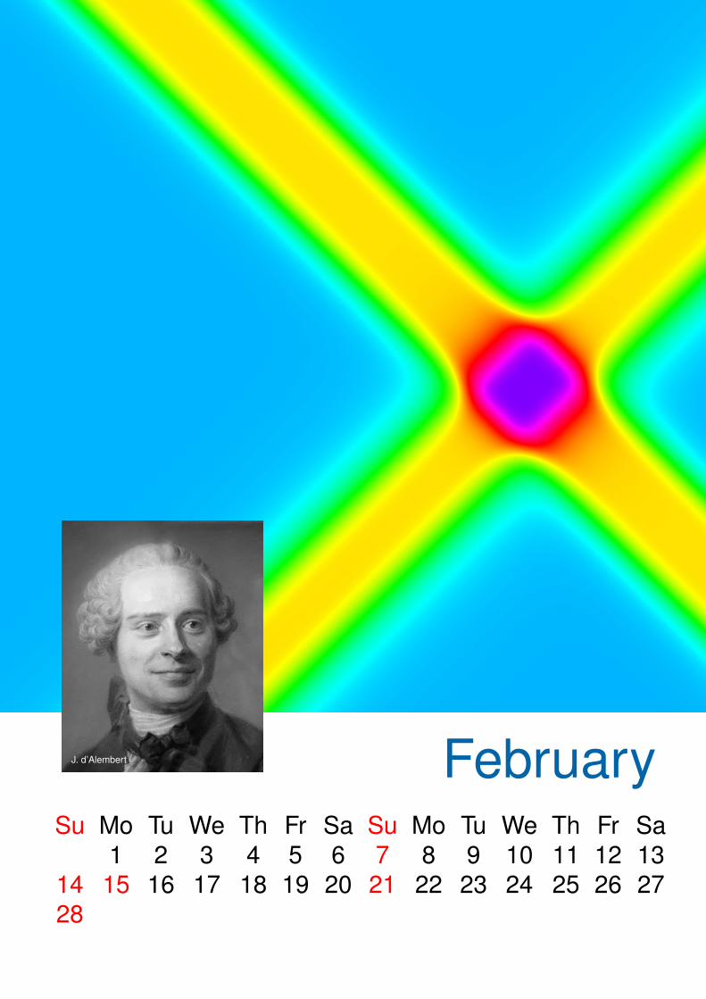
D’Alembert’s FormulaOne of the fundamental partial differential equations of mathematical physics is the one-dimensionalwave equation for a function u(t, x):

utt(t, x) = c2uxx(t, x).

This equation could describe the vibration of a string at time t and the location x, for instance, orit may represent the mechanical tension in a longitudinally extended rod. The positive constant cdepends on the material properties of the string or the rod. Allowing the interval of consideration toextend to infinity, we may take x to be any real number. Displacement and displacement velocity attime t = 0 are prescribed by the functions

u(0, x) = ϕ(x) and ut(0, x) = ψ(x).

The solution of this initial value problem is given by d’Alembert’s formula

u(t, x) =12(ϕ(x− ct) + ϕ(x + ct)) +

12c

∫ x+ct

x−ctψ(s) ds.

Denoting an antiderivative of ψ by Ψ we may express this formula as

u(t, x) =12(ϕ(x− ct) + ϕ(x + ct)) +

12c

(Ψ(x + ct)−Ψ(x− ct)) .

Thus, the solution is a superposition of four waves with two of them propagating to the left, twoof them propagating to the right, and all of them with constant speed of propagation c. By twos,these waves are shifts along the x-axis of otherwise identical-looking function graphs. The picture

x

x 7→ ϕ(x + ct2)x 7→ ϕ(x + ct3) x 7→ ϕ(x + ct1)

on the left shows the graph of x 7→ ϕ(x + ct)for three values t1 < t2 < t3. The picture ofthe month shows exp(iu) as a function of thecomplex variable x + it for ψ ≡ 0. Here onlytwo propagating waves intersect each other.

Jean Le Rond d’Alembert (1717 – 1783)was abandoned on the steps of Saint Jean Le Rond (at the time a side chapel of Notre-Dame deParis) by his mother Claudine Guerin de Tencin, a salonniere. The artillery officer Louis CamusDestouches made sure he found a home, got a good education, and, in 1726, at Destouches’ deathhe left d’Alembert with a lifelong allowance. Because of this, for a long time he was assumed to bed’Alembert’s father. Newer theories speculate that Destouches acted on behalf of the imperial fieldmarshal Duke of Arenberg. In fact, d’Alembert went by the name of Jean d’Aremberg and only laterchanged it to Jean d’Alembert.

While attending the College des Quatre-Nations, d’Alembert augmented his mathematics lessonswith self-study but decided on a career in law. He earned his law degree in 1738 and turned tomedicine briefly before settling on mathematics. In 1739 he presented his first paper to the Academiedes Sciences in Paris and two years later he was admitted to this academy. In 1754, he was elected tothe Academie Francaise, the French literary academy. But he declined the presidency of the BerlinerAkademie der Wissenschaften.

D’Alembert worked in fluid dynamics and mechanics (d’Alembert’s prinicple of inertial forces). In1747 he published the wave equation. Together with Diderot he became editor of the Encyclopediefor which he wrote more than 1700 articles, most of them in the sciences. He defined the derivativeas a limit of difference quotients and he discovered the ratio test for the convergence of a series.D’Alembert contributed to the proof of the fundamental theorem of algebra, which is often namedafter him in French. In addition, he published in the theory of music, astronomy, and philosophy, andhe translated antique scripts from Latin into French. Since he was an avowed atheist he was buriedin an unmarked grave.Francoise Launay: Les identites de D’Alembert, Recherches sur Diderot et sur l’Encyclopedie, 47, 2012, accessed 8/18/2020 on http://journals.openedition.org/rde/4949.

D. Bernoulli MarchSu Mo Tu We Th Fr Sa Su Mo Tu We Th Fr Sa

1 2 3 4 5 6 7 8 9 10 11 12 1314 15 16 17 18 19 20 21 22 23 24 25 26 2728 29 30 31

Plane Waves and their SuperpositionVibrating strings were first studied by Jean Le Rond d’Alembert, Leonhard Euler, Daniel Bernoulli,and Joseph-Louis Lagrange, among others. The one-dimensional wave equation was discoveredin 1746 by d’Alembert (see February). Here we consider the version that is two-dimensional withrespect to space:

utt(t, x, y) = c2 (uxx(t, x, y) + uyy(t, x, y))

,

where c is a positive real constant. A solution of this partial differential equation is a function u(t, x, y)with t a time parameter and x and y space parameters.

The wave equation is linear, which means that if u1(t, x, y) and u2(t, x, y) are two solutions of theequation, then for all constants a1 and a2, the linear combination a1u1(t, x, y) + a2u2(t, x, y) is also asolution. This fundamental insight is called the superposition principle. According to Leon Brillouin, itwas first stated by Daniel Bernoulli in 1753.

On the left and in the middle of the pictures inset below are two basic solutions u1(t0, x, y) andu2(t0, x, y) at some fixed time t0. The waves propagate in the direction of the arrows and both havethe same amplitude. The superposition u1(t0, x, y) + 1.5u2(t0, x, y) at the same time t0 appears onthe right. This month’s title picture shows the same function but uses grey tones to highlight the wavepropagation.

Waves are of fundamental importance in many fields of physics and engineering. There are lightwaves, sound waves, water waves; and waves occur in electromagnetics, fluid dynamics, quantummechanics, geophysics, and many other fields. Shortly after d’Alembert’s discovery, Euler generali-zed to the three-dimensional wave equation. Since it is still a linear partial differential equation, thesuperposition principle holds, even though Euler did not think so at first. It was Fourier who helpedthe principle gain widespread acceptance.

Daniel Bernoulli (1700 – 1782)was born in Groningen, in the Netherlands. When he was five, the family returned to their native townof Basel, Switzerland. His father made him study medicine but taught him mathematics on the side.After studying in Basel, Heidelberg, and Strasbourg, Daniel graduated with a PhD in anatomy andbotany and a deep understanding of mathematics.

In 1725, Daniel and his brother Nicolaus II went to St. Petersburg where they both held professor-ships in mathematics. But, within a year of their arrival, his brother died. To lessen Daniel’s despair,his father sent him one of his pupils to St. Petersburg – a friend of Daniel’s from Basel by the nameof Leonhard Euler. The two of them worked closely together and it was the time of Daniel’s bestwork. Nevertheless, Daniel was very unhappy in this rough climate and in 1733 he returned to Basel,where he held positions at the university, first in botany, then in physiology, and finally in physics.

Daniel is one of the eight outstanding mathematicians of the Bernoulli family, including his fatherand his two brothers. But his father was jealous of his son’s work and their relationship deteriorated.Daniel Bernoulli worked in many areas of mathematics and physics, he is known for the Bernoulliprinciple, and his main work is the book Hydrodynamica. He was an elected member of most of theleading scientific societies and he won the Grand Prize of the Paris Academy ten times.Brillouin, L. Wave propagation in periodic structures, Dover 2003.J. J. O’Connor and E. F. Robertson, Daniel Bernoulli, MacTutor History of Mathematics, (University of St Andrews, Scotland, 1998).

H. Hankel AprilSu Mo Tu We Th Fr Sa Su Mo Tu We Th Fr Sa

1 2 3 4 5 6 7 8 9 1011 12 13 14 15 16 17 18 19 20 21 22 23 2425 26 27 28 29 30

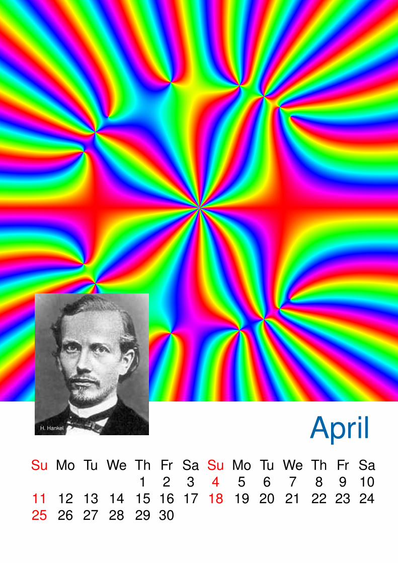
The Hankel DeterminantIn his thesis, Hankel introduced objects that are now known as Hankel matrices, or square matricesin which the elements on the skew-diagonal from lower left to upper right are constant. A 4× 4 Hankelmatrix looks like this:

a b c db c d ec d e fd e f g

Hankel matrices appear in various settings, often making an appearance when using the relationshipbetween polynomials and matrix computations to develop numerical algorithms. In particular, then × n matrix Hn = (Hij) where Hij = 1/(i + j − 1), called the Hilbert matrix, is an example ofa Hankel matrix. Matrices of the form Hn were studied by Hilbert in connection with a problem inapproximation theory and studied extensively in the early days of digital computing.

In his thesis, Hankel also discussed the computation of determinants of Hankel matrices. Deter-minants are computed using the entries of the matrix and can be defined recursively, beginning withthe determinant of a 2× 2 matrix:

det(

a bc d

)= ad− bc.

Determinants encode properties of the matrix; for example, det(A) = 0 if and only if the matrix A issingular. The determinant of the Hilbert matrix is known to be:

det (Hn) =(1!2! · · · (n− 1)!)4

1!2! · · · (2n− 1)!∼ 2−2n2

.

You can see that for n large, this determinant is very close to zero, and so numerical algorithmsmay show that the matrix is singular. However, theoretical computations show that the determinant isactually always positive. This month’s picture shows the Hankel determinant introduced in Hankel’sthesis for a 3× 3 matrix. Hankel’s choice of the entries, which are functions of a variable z, makeseven this low-degree case somewhat complicated. The function is displayed in the square |Re z| <1.5, |Im z| < 1.5.

Hermann Hankel (1839 – 1873)was born in Halle, Germany. He attended the University of Leipzig, where he studied under MoritzDrobisch, August Ferdinand Mobius, and his own father, Wilhelm Gottlieb Hankel. He also studiedin Gottingen, where he was a student of Riemann. In addition, he studied with Weierstrass andKronecker in Berlin. He held positions in Leipzig, Erlangen, and Tubingen.

Hankel worked on the theory of complex numbers, function theory, and the history of mathema-tics. In addition to Hankel matrices (and operators), his name is also attached to the Hankel trans-form. This transform is one that expresses a given function as a weighted sum of an infinite number ofBessel functions of the first kind and it appears when writing the multidimensional Fourier transformin hyperspherical coordinates. For this reason, it is often useful in problems that involve cylindricalor spherical symmetry. Hankel is also known for his work, Theorie der complexen Zahlensysteme,published in 1867, in which he both recognized the importance of Hermann Grassman’s work andhelped make these ideas better known. In function theory, his main contributions included reformu-lating Riemann’s criterion for integrability, “placing the emphasis upon measure-theoretic propertiesof sets of points. . . . Although he confounded the notions of sets of zero content and nowhere-densesets, his work marked an important advance toward modern integration theory.” He died on August29, 1873 in Schramberg, in the Black Forest in Germany.

https://www.encyclopedia.com/science/dictionaries-thesauruses-pictures-and-press-releases/hankel-hermann.

V. N. Faddeeva MaySu Mo Tu We Th Fr Sa Su Mo Tu We Th Fr Sa

1 2 3 4 5 6 7 89 10 11 12 13 14 15 16 17 18 19 20 21 2223 24 25 26 27 28 29 30 31

Vera Faddeeva and the w-Function (by Andre Weideman)The function defined by

w(z) = e−z2erfc(−iz) = e−z2

(1 +

2i√π

∫ z

0et2

dt)

, z ∈ C

goes by many names: plasma dispersion function, complex error function, Kramp function, Faddeevafunction, or simply w-function. Equally numerous are the fields of application: plasma waves, dilutedgases, subatomic particles, spectroscopy, and many others.

The w-function is related to the Mittag-Leffler function, namely w(z) = E1/2(iz) (CB July 2014).It can also be obtained as a Hilbert transformation of the Gauss function (density function of thenormal distribution) or, equivalently, the convolution of the Gauss function with the density functionof the Cauchy-Lorentz distribution. These integral representations are the basis of many numericalalgorithms for the calculation of values w(z). It was also the concept used by Vera Faddeeva and hercolleague N.M. Terentev for their impressive work “Tables of values of the function w(z) for complexargument” that appeared in 1954 in Russian and was translated into English in 1961.

Gauss’ error function, erf, and w are both entire functions. The decision to tabulate the w-function,rather than one of the other related ones, was likely made because from the values of the w-functionin the first quadrant one can easily derive the values at all other places as well as the values for theerror function erf, the Dawson integral, the Fresnel integrals (CB October 2013), the Voigt functions,and several others.

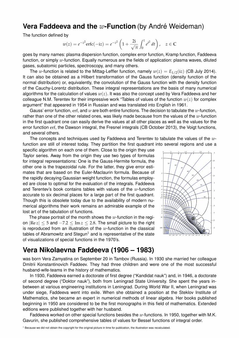
The concepts and techniques used by Faddeeva and Terentev to tabulate the values of the w-function are still of interest today. They partition the first quadrant into several regions and use aspecific algorithm on each one of them. Close to the origin they useTaylor series. Away from the origin they use two types of formulasfor integral representations: One is the Gauss-Hermite formula, theother one is the trapezoidal rule. For the latter, they give error esti-mates that are based on the Euler-Maclaurin formula. Because ofthe rapidly decaying Gaussian weight function, the formulas employ-ed are close to optimal for the evaluation of the integrals. Faddeevaand Terentev’s book contains tables with values of the w-functionaccurate to six decimal places for a large part of the first quadrant.Though this is obsolete today due to the availability of modern nu-merical algorithms their work remains an admirable example of thelost art of the tabulation of functions.

The phase portrait of the month shows the w-function in the regi-on |Re z| ≤ 5 and −7.2 ≤ Im z ≤ 2.8. The small picture to the rightis reproduced from an illustration of the w-function in the classicaltables of Abramowitz and Stegun1 and is representative of the stateof visualizations of special functions in the 1970’s.

.2

.3

.4

.5

.6

.7

.8

.91.0

2

345

10

100

10◦20◦

30◦

40◦

50◦

60◦

70◦

80◦

90◦

120◦60◦0◦−60◦−120◦±180◦120◦60◦0◦−60◦−120◦±180◦120◦

0 .5 1 1.5 2 2.5 3

−2

−1.5

−1

−.5

0

.5

1

1.5

2

2.5

3

Vera Nikolaevna Faddeeva (1906 – 1983)was born Vera Zamyatina on September 20 in Tambov (Russia). In 1930 she married her colleagueDmitrii Konstantinovich Faddeev. They had three children and were one of the most successfulhusband-wife-teams in the history of mathematics.

In 1930, Faddeeva earned a doctorate of first degree (“Kandidat nauk”) and, in 1946, a doctorateof second degree (“Doktor nauk”), both from Leningrad State University. She spent the years in-between at various engineering institutions in Leningrad. During World War II, when Leningrad wasunder siege, Faddeeva went into exile. When she obtained a position at the Steklov Institute ofMathematics, she became an expert in numerical methods of linear algebra. Her books publishedbeginning in 1950 are considered to be the first monographs in this field of mathematics. Extendededitions were published together with her husband.

Faddeeva worked on other special functions besides the w-functions. In 1950, together with M.K.Gavurin, she published comprehensive tables of values for Bessel functions of integral order.1 Because we did not obtain the copyright for the original picture in time for publication, the illustration was recalculated.

E. K. Abbe JuneSu Mo Tu We Th Fr Sa Su Mo Tu We Th Fr Sa

1 2 3 4 5 6 7 8 9 10 11 1213 14 15 16 17 18 19 20 21 22 23 24 25 2627 28 29 30

The Poisson Point ProcessA point process is a procedure to distribute points randomly in a one- or multi-dimensional region B,for instance in a square. A Poisson point process is characterized by two properties:

– The points do not influence each other; that is, their positions are stochastically independent.– The random number of points in a subset M of B has a Poisson distribution with parameter

λ(M) (compare CB June 2020).Here λ is a measure on B, called the intensity measure of the process. If λ(B) is finite, then theprobability that M will be hit by a point is λ(M)/λ(B). If λ(M) is proportional to the volume of Mthen we call it a homogeneous or stationary Poisson process.

Even though Simeon Denis Poisson never studied this process, it was named after him dueto its connection to the Poisson distribution. One of the pioneers in analyzing the process wasErnst Abbe. In 1879, he studied the reliability of a microscopic instrument used to count bloodcells. Further developments are attributed to Andrey Kolmogorov (CB September 2020), NorbertWiener, William Feller, Aleksandr Khinchin and Paul Levy.

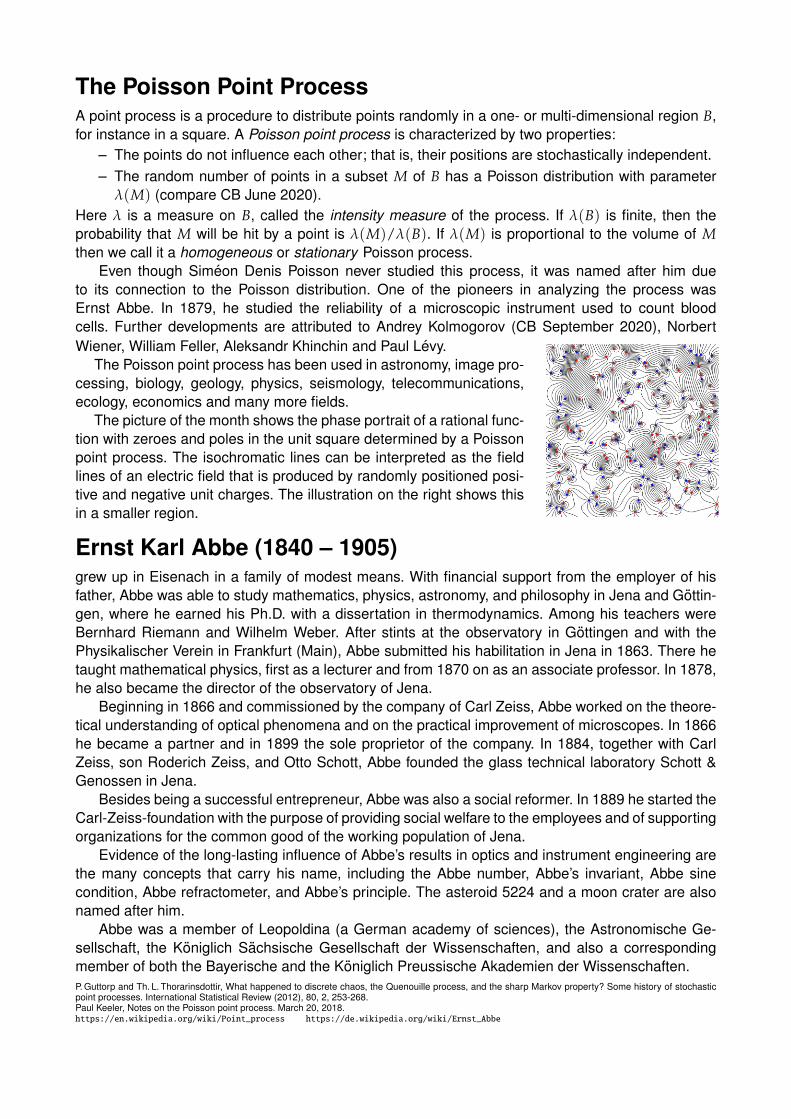
The Poisson point process has been used in astronomy, image pro-cessing, biology, geology, physics, seismology, telecommunications,ecology, economics and many more fields.

The picture of the month shows the phase portrait of a rational func-tion with zeroes and poles in the unit square determined by a Poissonpoint process. The isochromatic lines can be interpreted as the fieldlines of an electric field that is produced by randomly positioned posi-tive and negative unit charges. The illustration on the right shows thisin a smaller region.

Ernst Karl Abbe (1840 – 1905)grew up in Eisenach in a family of modest means. With financial support from the employer of hisfather, Abbe was able to study mathematics, physics, astronomy, and philosophy in Jena and Gottin-gen, where he earned his Ph.D. with a dissertation in thermodynamics. Among his teachers wereBernhard Riemann and Wilhelm Weber. After stints at the observatory in Gottingen and with thePhysikalischer Verein in Frankfurt (Main), Abbe submitted his habilitation in Jena in 1863. There hetaught mathematical physics, first as a lecturer and from 1870 on as an associate professor. In 1878,he also became the director of the observatory of Jena.

Beginning in 1866 and commissioned by the company of Carl Zeiss, Abbe worked on the theore-tical understanding of optical phenomena and on the practical improvement of microscopes. In 1866he became a partner and in 1899 the sole proprietor of the company. In 1884, together with CarlZeiss, son Roderich Zeiss, and Otto Schott, Abbe founded the glass technical laboratory Schott &Genossen in Jena.

Besides being a successful entrepreneur, Abbe was also a social reformer. In 1889 he started theCarl-Zeiss-foundation with the purpose of providing social welfare to the employees and of supportingorganizations for the common good of the working population of Jena.

Evidence of the long-lasting influence of Abbe’s results in optics and instrument engineering arethe many concepts that carry his name, including the Abbe number, Abbe’s invariant, Abbe sinecondition, Abbe refractometer, and Abbe’s principle. The asteroid 5224 and a moon crater are alsonamed after him.

Abbe was a member of Leopoldina (a German academy of sciences), the Astronomische Ge-sellschaft, the Koniglich Sachsische Gesellschaft der Wissenschaften, and also a correspondingmember of both the Bayerische and the Koniglich Preussische Akademien der Wissenschaften.P. Guttorp and Th. L. Thorarinsdottir, What happened to discrete chaos, the Quenouille process, and the sharp Markov property? Some history of stochasticpoint processes. International Statistical Review (2012), 80, 2, 253-268.Paul Keeler, Notes on the Poisson point process. March 20, 2018.https://en.wikipedia.org/wiki/Point_process https://de.wikipedia.org/wiki/Ernst_Abbe

W. K. Hayman JulySu Mo Tu We Th Fr Sa Su Mo Tu We Th Fr Sa

1 2 3 4 5 6 7 8 9 1011 12 13 14 15 16 17 18 19 20 21 22 23 2425 26 27 28 29 30 31

The Growth of Entire FunctionsA function f is said to be entire if it is holomorphic in the whole complex plane C. Typically, thefunction values f (z) of entire functions grow rapidly as |z| → ∞. If an entire function f is boundedon C, then f is constant (Liouville’s theorem). For a more in-depth analysis of the growth propertiesof entire functions one considers their maxima and minima on circles of radius r,

M(r, f ) = max{| f (z)| : |z| = r}, m(r, f ) = min{| f (z)| : |z| = r}.If the growth of M(r, f ) as r → ∞ is not faster than the growth of rn for some positive integer n, thenf is a polynomial of degree at most n. Interesting questions arise when M(r, f ) grows faster thanany power of r.

It was noted early on that m(r, f ) and M(r, f ) are not independent of each other. But an exactdescription of their relationship turned out to be difficult. In 1918, Anders Wiman conjectured that foreach entire function f and each positive ε there exists an arbitrarily large r such that

m(r, f ) > M(r, f )−1−ε.

It wasn’t until 1952 that Walter Hayman disproved this conjecture by constructing an intricate coun-terexample. Hayman’s function f has the form of an infinite product whose factors are scaled powersof a special “base function.” The zeroes of these factors are on rays emanating from the origin. Theirmultiplicities double from one factor to the next. The images below are modified phase portraits of theproducts f3, f5, and f7 with 3, 5, and 7 factors, respectively. Dark (light) colors correspond to small(large) values of | f |. The picture of the month shows a pure phase portrait of f7 in which the zerosand their multiplicities are clearly visible.

Walter Kurt Hayman (1926 – 2020)was born in Koln, where his father was a law professor. His maternal grandfather was the mathema-tician Kurt Hensel, himself the grandson of the composer Fanny Hensel, nee Mendelssohn. BecauseHayman’s father was Jewish, his father lost his position in 1935, and in 1938 the family fled to GreatBritain. In Scotland, Hayman attended the famous Gordonstoun School that was founded by KurtHahn, a nephew of his mother. At St. John’s College of Cambridge University Hayman studied withJohn E. Littlewood (CB April 2018) and Mary Cartwright (CB April 2016). The latter became his the-sis advisor. After positions in Newcastle and Exeter, Hayman was appointed to a professorship atthe Imperial College in London in 1956. After his retirement in 1985 he took a part-time position atthe University of York until 1993. Beginning in 1995 he was a Senior Research Fellow at the ImperialCollege again.

Hayman’s fields of work were function and potential theory. He published more than 200 papers,among them a proof of the asymptotic Bieberbach conjecture and the “Hayman alternative” in Nev-anlinna theory. Among his influential books are “Multivalent Functions” (1958, 1994), “MeromorphicFunctions” (1964), “Subharmonic Functions” (1976, 1989), “Research Problems in Function Theory”(1967, 2019), and his autobiography “My Life and Functions” (2014). Since 1956 he was a memberof the Royal Society and he was an invited speaker at the International Congress of Mathematicianstwice. Inspired by a visit to Moscow and together with his wife Margaret Hayman he founded theBritish Mathematical Olympiad in 1966.

St. Ruscheweyh AugustSu Mo Tu We Th Fr Sa Su Mo Tu We Th Fr Sa1 2 3 4 5 6 7 8 9 10 11 12 13 1415 16 17 18 19 20 21 22 23 24 25 26 27 2829 30 31

Ruscheweyh DerivativesConsider two functions, f and g, holomorphic on the unit disk D. Their Hadamard product, denotedf ∗ g, is defined using the power series representations as follows:

f (z) =∞

∑k=0

akzk, g(z) =∞

∑k=0

bkzk, ( f ∗ g)(z) =∞

∑k=0

akbkzk.

Ruscheweyh and Sheil-Small showed that the Hadamard product preserves the class of convexfunctions (that is, the class of univalent conformal mappings of the unit disk onto convex domains).The Ruscheweyh derivative, which was introduced by Ruscheweyh in connection with this work, isdefined for α > −1 by

Dα f (z) =z

(1− z)α+1 ∗ f (z).

In case α = n is a positive integer, the Ruscheweyh derivative can indeed be expressed in terms ofthe usual derivative, namely

Dn f (z) =zn!

dn

dzn

(zn−1 f (z)

).

If f (0) = 0, then we also have D0 f = f (not however, if f (0) , 0). The Ruscheweyh derivatives arerelated to geometric properties of conformal maps.

The inset figure below shows the phase plot of the tangent function f (z) = tan z on the left, itsRuscheweyh derivative D1 f in the middle, and D2 f on the right. These are graphed in the square|Re z| < 7, |Im z| < 7. The picture of the month is D5 f for the same function f .

Stephan Ruscheweyh (1944 – 2019)was born in Zwickau, a town in Saxony, Germany. He studied in Freiburg, Kiel, and Bonn and hisfirst position was an associate professorship at the University of Dortmund. He then became a fullprofessor at the University of Wurzburg, where he remained until his retirement in 2012.

Between 1973 and 1980 Ruscheweyh held visiting positions at the University of Kabul. Afterthe end of the Taliban regime, he returned there almost yearly. During the time in which visits toAfghanistan were impossible, Ruscheweyh directed activities in India, Nepal, Chile, Canada, and theUSA. He spent a great deal of time in Chile, where he worked with his frequent collaborator, LuisSalinas. It was in Chile that the idea to create “Computational Methods in Function Theory” (CMFT)conferences first arose; so far there have been eight such conferences, each one in a differentcountry. Ruscheweyh also played a key role in founding the journal by the same name.

In his obituary, his colleagues write, “Stephan had a true gift of understanding and explainingthe interdependence of algebra, analysis, and geometry, using tools from convolution theory, diffe-rential equations, special function theory, operator theory, and approximation theory.”1 He served assupervisor for 13 Ph.D. students.1. R. Barnard, W. Bergweiler, I. Laine, Computational Methods and Function Theory (2019) 19:541–544.

J.-P. Kahane SeptemberSu Mo Tu We Th Fr Sa Su Mo Tu We Th Fr Sa

1 2 3 4 5 6 7 8 9 10 1112 13 14 15 16 17 18 19 20 21 22 23 24 2526 27 28 29 30

Random Power SeriesA random variable is a variable Z whose values depend on outcomes of a random phenomenon.For example, if tossing a fair six-sided die, the number showing, Z, is a random variable. It takeson the values k = 1, . . . , 6, each with probability P(Z = k) = 1/6. For some random variables,the probability that one particular number occurs is zero. In these cases we have to ask for theprobability that a particular value belongs to a (Borel) subset A ⊆ C. If this probability is given by

P(Z ∈ A) =1

2π

∫A

e−|z|2/2dσ(z),

where dσ denotes Lebesgue measure, then the random va-riable Z has a (standard) normal distribution. The integralmay be interpreted as the volume of the solid above A andbelow the Gaussian bell-shaped surface (image to the right).

We now focus on power series with random coefficients; more precisely, power series of the form

F(z) =∞

∑n=0

Zn an zn, (1)

where Zn are independent and normally distributed random variables and an are fixed positive realnumbers satisfying lim supn→∞

n√

an = 1. The latter condition ensures that the radius of convergenceof the deterministic power series ∑ anzn is 1. That is, this series converges if |z| < 1 and it divergesif |z| > 1. The radius of convergence R of the series (1) is a random variable and F is a randomfunction.

It can be shown that we have R = 1 with probability 1; that is, the event R = 1 happens almostsurely. Likewise it is almost surely the case that the natural boundary of F(z) is the unit circle T,meaning that F cannot be continued analytically past any arc of T. If ∑ a2

n < ∞, then the series (1)will converge almost surely almost everywhere on T. On the other hand, if ∑ a2

n = ∞, then F willbehave very wildly at the boundary of the unit disk: the series (1) will almost surely diverge almosteverywhere on T. In the latter case, according to a theorem by Kahane, f (D) fills the whole complexplane.

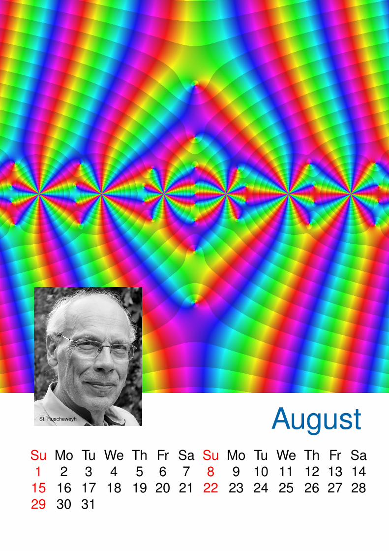
The picture of the month shows the result of such a random experiment with an = 1/√

n. Forthe series (1) we used the first 1000 terms. In this case, ∑ a2

n is the divergent harmonic series –the emergence of the natural boundary of the function F is already clearly visible in the picture. Incoloring the phase portrait we used brightness to show the modulus of the function values; in regionsthat are almost white, the modulus is very large.

Jean-Pierre Kahane (1926 – 2017)was born in Paris, the son of a professor of biochemistry. He studied at the Ecole normale superieurin Paris. He started research at the Centre national de la recherche scientifique, and, in 1954, heearned a Ph.D. under the supervision of Szolem Mandelbrojt. That same year, he started as a lecturerat L’Universite de Monpellier eventually becoming a professor. In 1961 he moved to the UniversiteParis-Sud, Orsay, where he stayed to his retirement in 1994.

Despite his extensive scientific work, Kahane held several administrative positions. Among themwere the presidency of the Societe mathematique de France (1972–1973), the presidency of the Uni-versite Paris-Sud, Orsay (1975–1978), and membership of the Academie des sciences. Throughouthis life he was a very engaged member of the French communist party.

Kahane’s main areas of research were harmonic analysis and Fourier series (e.g., the Kahane–Katznelson–de-Leeuw theorem: to (cn) ∈ `2 there is a continuous function f with Fourier coefficients| f (n)| ≥ |cn|), functional analysis (e.g., the theorem of Gleason-Kahane-Zelazko about the charac-terization of multiplicative linear functionals on a complex Banach algebra), probabilistic methodsin analysis and Brownian motion (e.g., proving properties of Mandelbrot martingales), and numbertheory (e.g., a proof of the Bateman-Diamond conjecture about Beuerling generalized primes).S.-P. Kahane: Some random series of functions, 2nd edition, Cambridge University Press 1985.J. Barral, J. Peyriere, H. Queffelec: ICMI column – the mathematical legacy of Jean-Pierre Kahane. Eur. Math. Soc. Newsl. No. 108 (2018), 43–47.

E. Schroder OctoberSu Mo Tu We Th Fr Sa Su Mo Tu We Th Fr Sa

1 2 3 4 5 6 7 8 910 11 12 13 14 15 16 17 18 19 20 21 22 2324 25 26 27 28 29 30 31

Schroder’s Functional EquationIn a paper entitled Ueber iterierte Functionen published in Mathematische Annalen in 1870, Schroderintroduced what is now called Schroder’s functional equation:

f ◦ ϕ = s f , where ϕ and f are functions and s is a constant.

In the context of a composition operator Cϕ that acts on some function space and is defined byCϕ( f ) = f ◦ ϕ, Schroder’s equation can be viewed as the eigenvalue equation of the operator:Cϕ( f ) = s f . Composition operators play an important role in mathematics and have been studiedextensively. The original proof of the Bieberbach conjecture depended on composition operators andthey are fundamental to the theory of dynamical systems.

In his 1870 paper, Schroder was interested in explicit formulas for the iteration of a function. Hewas looking for functions ϕ and f satisfying his functional equation with the additional property that fwould be invertible in at least some domain. In this case we have ϕ = f−1 ◦ (s f ), which gives rise tothe iteration ϕn = f−1 ◦ (sn f ). He did not come up with a general theory but he gave some interestingexamples, one of them being the function ϕ(z) = 2z/(1 + z2). He showed that for this function s = 2and f (z) = arctan(iz). Below we show the phase portraits, enhanced with the modulus for Schroder’sexample ϕ, f , f−1, and the composition f−1 ◦ (2 f ). The latter is the same as the function ϕ. Iteratedfunctions are central objects in the study of fractals and in the theory of dynamical systems. Theyare widely applied in computer science and in physics.

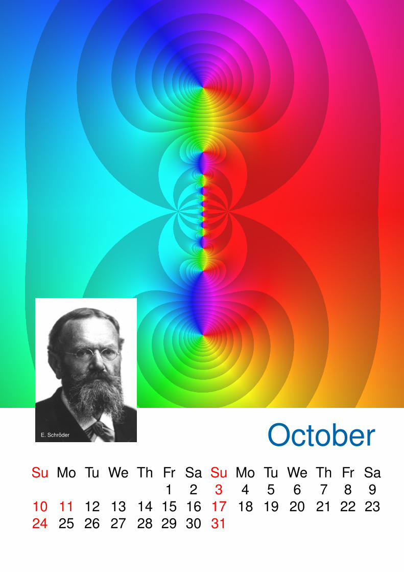
This month’s cover image is the phase portrait with the modulus of the third iteration of Schroder’sfunction introduced above, ϕ3 = f−1 ◦ (8 f ) on |Re z| < 8 and |Im z| < 8.

Friedrich Wilhelm Karl Ernst Schroder (1841 – 1902)was born the son of a science teacher at a gymnasium in Mannheim. For two years, when he wasyoung, Ernst lived with his maternal grandfather, a pastor, who gave him a solid educational basiswith emphasis on Latin. Also influenced and taught by his father, Ernst Schroder showed exceptionaltalent in languages, sciences, and mathematics. After graduating from the Lyceum in Mannheim,he studied in Heidelberg, earning his Ph.D. in 1862 in mathematics with Otto Hesse as his advi-sor. Schroder spent two years studying mathematical physics in Konigsberg, before submitting hishabilitation at the ETH in Zurich, Switzerland. He stayed there for four years working as a lecturerand climbing difficult routes in the Swiss alps. In 1870, he returned to Germany, first as a teacherin a gymnasium, then as professor in Darmstadt, and eventually as professor of mathematics at theTechnische Hochschule in Karlsruhe where he remained for the next 33 years to his death.

Schroder started out being interested in mathematical physics and his early paper cited abovewas fundamental for the new field of dynamical systems. But his interest soon shifted to logic. Hethought of himself as a (Boolean) algebraist and he developed a system of logical calculus. His threevolume work “Vorlesungen uber die Algebra der Logik” (Lectures on the algebra of logic) was finishedposthumously and turned out to be very influential.

Schroder is described as having been a gentle even-tempered person. He was active in manydifferent sports and was often seen biking all over Karlsruhe and its surroundings. He never marriedand gave his full attention to his position at the Technische Hochschule, where he was the directorfor the year 1890-91.C. C. Cowen, B. D. MacCluer, Composition Operators on Spaces of Analytic Functions, CRC Press, Boca Raton, FL, 1995.J. J. O’Connor and E. F. Robertson, Ernst Schroder, MacTutor History of Mathematics, (University of St Andrews, Scotland, 2009).

E. Ising NovemberSu Mo Tu We Th Fr Sa Su Mo Tu We Th Fr Sa

1 2 3 4 5 6 7 8 9 10 11 12 1314 15 16 17 18 19 20 21 22 23 24 25 26 2728 29 30

The Ising Model and Painleve Functions (by Marco Fasondini)

The phenomenon of ferromagnetism (permanent magnets) had to await breakthroughs in quantumand statistical mechanics in the 1920s and 1940s before it could be understood from first principles.Before this, Wilhelm Lenz, who had proposed a quantum mechanical model for ferromagnetism in1920, assigned his doctoral student Ernst Ising the task of explaining the appearance of a ferroma-gnetic state in a three-dimensional (3D) solid. Ising’s 1924 thesis presented a 1D quantum statisticalmodel of elementary magnetic units and showed that ferromagnetism is not possible in his model.Ising entertained the possibility of ferromagnetism in higher dimensions but exact solutions to hismodel in 2D or 3D were not tractable at the time.

Onsager published the most interesting result in theoretical physics during the second world war(according to Pauli) when he derived an exact solution to the 2D Ising model. In 1948, Onsagerannounced after a talk that he and Kaufman had derived the spontaneous magnetisation of the2D Ising model. This established conclusively the existence of a phase transition from non-vanishingmagnetisation below the critical temperature (T < Tc) to vanishing magnetisation for T > Tc. Onsagerand Kaufman did not publish their result; Chen-Ning Yang was the first to do so in 1952.

In the 1970s, in the work of Barouch, McCoy, Tracy and Tai Tsun Wu, it was shown that the spin-spin correlation functions of the 2D Ising model can be expressed in terms of solutions to the thirdPainleve equation. This was among the first of the thenceforth numerous instances of a Painlevefunction (a nonlinear special function) in mathematical physics.

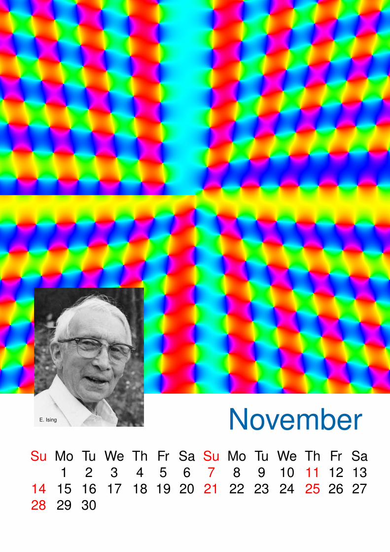
The Painleve equations are intro-duced in the month of November, 2014of the Complex Beauties calendar. Theimage on the right shows a solutionto the third Painleve equation that ap-pears in a spin-spin correlation func-tion of the 2D Ising model. The verti-cal spikes are the pole singularities ofthe solution. This month’s calendar pic-ture shows this same solution analyti-cally continued into another sheet of itsRiemann surface.

Ernst Ising (1900 – 1998)was born in Cologne to a Jewish mother and a gentile father. He studied mathematics and physicsat Gottingen and continued his studies at Bonn and Hamburg. He completed his doctoral researchin 1924 under the guidance of Wilhelm Lenz who at the time employed Pauli as his assistant. Apartfrom Ising’s 1950 paper “Goethe as Physicist”, he did not publish again after his doctoral thesis,however the model that bears his name has spawned tens of thousands of publications.

Ising worked for the patent office of General Electric in Berlin from 1925–26 after which he beca-me a high school teacher. He was headmaster of a school for Jewish children in Caputh near Pots-dam which was destroyed on Kristallnacht in 1938. In 1939, Ising was interrogated by the Gestapoand dismissed after he promised he and his wife would leave Germany. They fled to Luxembourgwhere their son was born. They had to postpone their planned emigration to the US until after the warbecause of a quota on US immigration. Ising was one of only 36 Jews in Luxembourg who were notdeported because of a secret directive by Adolf Eichmann in 1942 to prepare for the deportation ofJews, “... except for Jewish spouses of German-Jewish married couples.” Ising and his family arrivedin New York in 1947. He spent a year as a teacher at the State Teacher’s College in Minot, NorthDakota, before he was appointed in 1948 as Professor of Physics at Bradley University in Peoria,Illinois, where he remained until his retirement in 1976.

H. Stahl DecemberSu Mo Tu We Th Fr Sa Su Mo Tu We Th Fr Sa

1 2 3 4 5 6 7 8 9 10 1112 13 14 15 16 17 18 19 20 21 22 23 24 2526 27 28 29 30 31

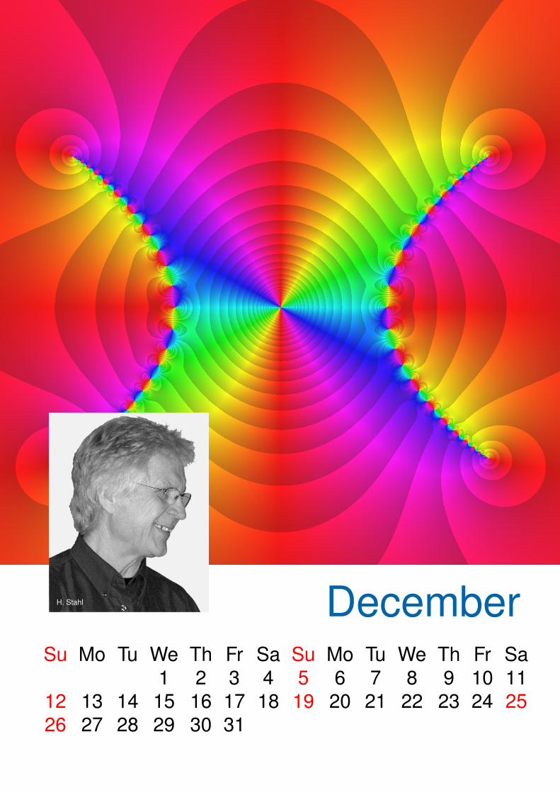
Natural Branch CutsIn an analytic continuation of a function one sometimes runs into the problem of multivalency: Con-tinuations along different paths lead to different outcomes. Among the simplest examples of thisphenomenon are the complex logarithmic function f (z) = log z (see CB May 2011) and generalpower functions f (z) = za (CB January 2011). To solve the problem one has two possibilities: Onecan look at the function on Riemann surfaces (CB December 2015) or introduce branch cuts (CBMarch 2018).

The Riemann surfaces are well-defined, but the placement of the branch cuts is somewhat ar-bitrary. It is standard to use the negative real line as the branch cut for the logarithmic function andits derived power functions. Using this convention we get the phase portrait below on the left for thefunction

f (z) =√(1− z1/z)(1− z2/z)(1− z3/z)(1− z4/z),

where z1 = −z2 = −z3 = z4 = eiπ/5. Interchanging the extraction of the root with the multiplication(totally allowable for real numbers), one obtains the phase portrait in the middle. Finally, the phaseportrait on the right belongs to the function

g(z) =√−i(1− z1/z)

√i(1− z2/z)

√i(1− z3/z)

√−i(1− z4/z).

Does there exist an “optimal” choice for a branch cut S? In a sequence of fundamental papers,Herbert Stahl answered this in the affirmative: To every function f meromorphic in a neighborhoodat infinity, there is a unique “extremal domain” G such that f can be extended meromorphically onG, where a domain G is called extremal (for f ), if S = C \ G is of the smallest possible “logarith-mic capacity” (a measure of its size). For the examples above, S is a system of “natural branchcuts” of the function extended out from infinity. This extension is, in fact, constructive. Certain Padeapproximations (see CB March 2017) of f at the point of infinity converge on G to the maximal me-romorphic continuation. The picture of the month shows such an approximation of f (and g): p/qwith deg p = 66 and deg q = 64. As the degree of the approximation increases, its zeroes and polesaccumulate along S, revealing the natural branch cuts. Here they consist of two arcs, connecting z1with z4 and z2 with z3.

Herbert Robert Stahl (1942 – 2013)was born in Fehl-Ritzhausen (Rheinland-Pfalz). From 1958 to 1964 he worked as an electrician. Aftera short stint as a sailor he studied at the Technische Universitat Berlin where he earned his Ph.D.working with Christian Pommerenke. In the middle of the 1980s he proved a 10-year-old conjectureby Nuttall about the convergence of Pade approximations. This brought him wide recognition.

Stahl’s main work was in function theory, approximation theory, potential theory and orthogonalpolynomials, but he also wrote papers in statistics and sociology. While in retirement, in 2011, heproved a 35-year-old conjecture about Hermitian matrices, known as the BMV conjecture.

Despite his two doctoral degrees, a habilitation, and being certified to lecture in mathematics,statistics, and electronic data processing, he did not obtain a professorship at the Technische Uni-versitat Berlin. He worked at the Technische Fachhochschule Berlin from 1986 until his retirement in2008.

A. Aptekarev, P. Nevai, V. Totik, In memoriam: Herbert Stahl August 3, 1942 – April 22, 2013. J. Approx. Theory 183 (2014) A1–A26.