jens kortus [email protected] tu...
TRANSCRIPT

Quantum Theory I
Jens Kortus [email protected]
TU Bergakademie Freiberg
Some recommendations : A.C. Phillips, Introduction to Quantum Mechanics Sakurai & Napolitano, Modern Quantum Mechanics Feynman, Lectures Greiner, Quantum Mechanics: An Introduction Konishi & Paffuti: Quantum Mechanics: A New Introduction many more

2
Warning! This script may contain errors. Warning! It is strongly recommended to check all derivations andFormulas themselves..
Please send any corrections and comments [email protected]
Pictures: If not stated explicitly otherwise, the pictures are fromhttp://de.wikipedia.org/ or have been created by the author.
3
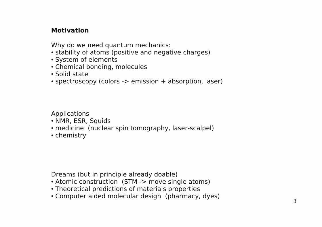
Why do we need quantum mechanics: stability of atoms (positive and negative charges) System of elements Chemical bonding, molecules Solid state spectroscopy (colors -> emission + absorption, laser)
Applications NMR, ESR, Squids medicine (nuclear spin tomography, laser-scalpel) chemistry
Dreams (but in principle already doable) Atomic construction (STM -> move single atoms) Theoretical predictions of materials properties Computer aided molecular design (pharmacy, dyes)
Motivation
4
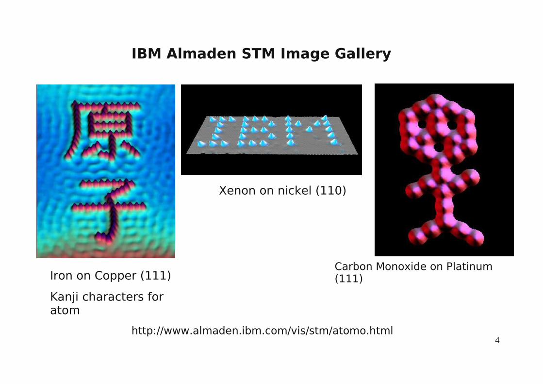
Xenon on nickel (110)
http://www.almaden.ibm.com/vis/stm/atomo.html
Carbon Monoxide on Platinum (111) Iron on Copper (111)
Kanji characters for atom
IBM Almaden STM Image Gallery

5
1. Some experimental observations1.1 Planck radiation law (black body radiation)
Thermal radiation (e.g. iron shows different colors with increasing temperature) IR (heat) → red → yellow → white
Interestingly, the colors depend only on temperature but not on the material.
T
Oven
Black body radiation: because there is no radiationat T = 0
Which frequencies and intensities will occur?
Rayleigh-Jeans law: classical electrodynamics (dipole radiation) and statistics (equal partition)
At thermal equilibrium each degree of freedom contains an energy of kT/2.
Calculation of the energy of the electromagnetic field in the oven Due to reflecting boundary conditions there will be standing electromagnetic waves Each wave has energy kT (kT/2 electric, kT/2 magnetic) , k=Boltzmann constant Need to count the number of such waves in a frequency interval [v + dv]

6
Cube with length a standing electric waves have minima at the walls standing magnetic waves have maxima at the walls
α
y
x
x cos=n1/2y cos =n2 /2z cos=n3/2
Standing waves are created, if they can fit an integer number times there wavelength/2 into the box.
λ/2
n1=2aλ cosα n2=
2aλ cosβ n3=
2aλ cosγ
using cos2α+cos2β+cos2 γ=1n1
2+n22+n3
2=(2 aλ )
2=(2a νc )
2 λ ν=c
ν= c2a √(n1
2+n22+n3
2)
Frequencies between 0 und v are within a sphere with radius 2av/c.However, there are only positive integer n, so that in case of a>>λ,the number of frequencies is equal to 1/8 of the volume of such sphere.
N (ν)=18
4 π3(2a νc)
3
d N (ν)=4 πa3 ν2
c3d ν
spectral energy densityωνd ν=2kT d N (ν)∼T ν2 d ν
7
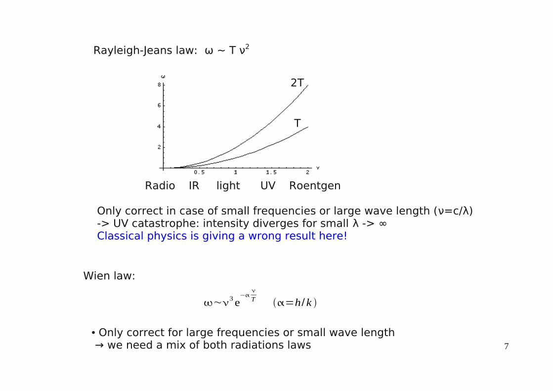
T
2T
Only correct in case of small frequencies or large wave length (ν=c/λ)-> UV catastrophe: intensity diverges for small λ -> ∞Classical physics is giving a wrong result here!
Rayleigh-Jeans law: ω ~ T ν2
Radio IR light UV Roentgen
Wien law:
~3 e−
T =h/k
Only correct for large frequencies or small wave length → we need a mix of both radiations laws

8
Planck radiation law (1900)
Interpolation between Rayleigh-Jeans and Wien law.
Interpretation: Atoms behave like harmonic oscillators and can only have discreteenergies
E=hv (n+ ½) = ћω (n+½)
The oscillators can only accept or emit energies equal to an integer n times a constant.
h = Planck quantum = 6.626 10-34 Js ћ=h/2π
ω∼ ν3
ehνkT−1
ν large(eh ν/kT≫1):∼ν3e−hνkT
νsmall(ex=1+ x+ ...):∼ν2kT
Max Karl Ernst Ludwig Planck* 23. April 1858 in Kiel † 4. Oktober 1947 in GöttingenNobelpreis 1918
9
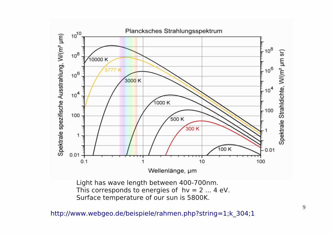
Light has wave length between 400-700nm.This corresponds to energies of hv = 2 ... 4 eV. Surface temperature of our sun is 5800K.
http://www.webgeo.de/beispiele/rahmen.php?string=1;k_304;1

10
1.2 Stability of atomsErnest Rutherford 1st Baron Rutherford of NelsonAugust 30, 1871 – October 19, 1937Nobelpreis Chemie 1908
Scattering of α-particles (He2+) at atoms in a gold foil.
+ Some α-particles were scattered back to the source. This means that there should be heavy positively charged centers in the gold.
According to classical pictures electrons move around the core like planets around the sun.However, movement along a circle is an accelerated motion. According to classical electrodynamics: Any accelerated charge will emit EM-radiation, which results in a loss of energy, so that the electron will fall into the core.This would result in a radiation decay of atoms during a time span of about 10-8 – 10-10 s.

11
1.3 Photoelectric effect
Metal plate in vacuum radiated with UV-light.
1) There is a minimal frequency for each metal below no photo-electrons can be found.2) Very fast process (<10-9s) 3) kinetic energy of the electrons for v>v
min
proportional to the frequency v of the light.4) Number of electrons proportional to intensity.
Explanation by Einstein 1905
Light = particles with energy E=hv (photon) Each photon kicks an electron from the metal. hv
min corresponds to the binding energy of the electron in the
metal. Electron number is proportional to the number of photons (intensity). Kinetic energy is proportional to h(v-v
min)
Albert Einstein* 14.3. 1879 Ulm † 18. 4. 1955 PrincetonNobelpreis Physik 1921

12
1.4 Particle-wave dualism
a) Wave character of lightInterference and diffraction (Huygens 1678)
Christiaan Huygens
* 14. April 1629 in Den Haag † 8. Juli 1695
Diffraction at single slit Double slit
Light is an electromagnetic field, fields can be superposed.
Er= E1 E 2
The intensity is the energy density ~ |E|2. Intensities can not be superposed. Picture is not sum of single pictures
I= E r⋅E r=∣ E r∣2=∣ E 1 E2∣
2≠∣ E1∣
2∣ E 2∣
2
b) Particle character of light -> see photo-electric effect

13
Waves of matter: de Broglie 1924 (Dissertation)
Applications: electron microscopy, Neutron scatteringQuantum optics, Quantum communication, Quantum computer, Quantum teleportation ...
All particles (atoms, molecules, solids) can have wave properties.
The de Broglie wave length of moving particles with momentum p is
λ=hp
Waves: Amplitude and phase, direction, polarization, wave length easy to measurematter-waves: direction in direction of momentum, de-Broglie Wellenlänge Phase velocity can not be measured
Louis-Victor Pierre Raymond de Broglie * 15. August 1892 in Dieppe, Normandie† 19. März 1987 in LouveciennesNobelpreis Physik 1929
Indivisibleness of particles: there will always be complete electrons in contrastto light (reflected and diffracted ray).
e.g. electrons with 10 keV kinetic energy have λ=0.12Å (Röntgen radiation).
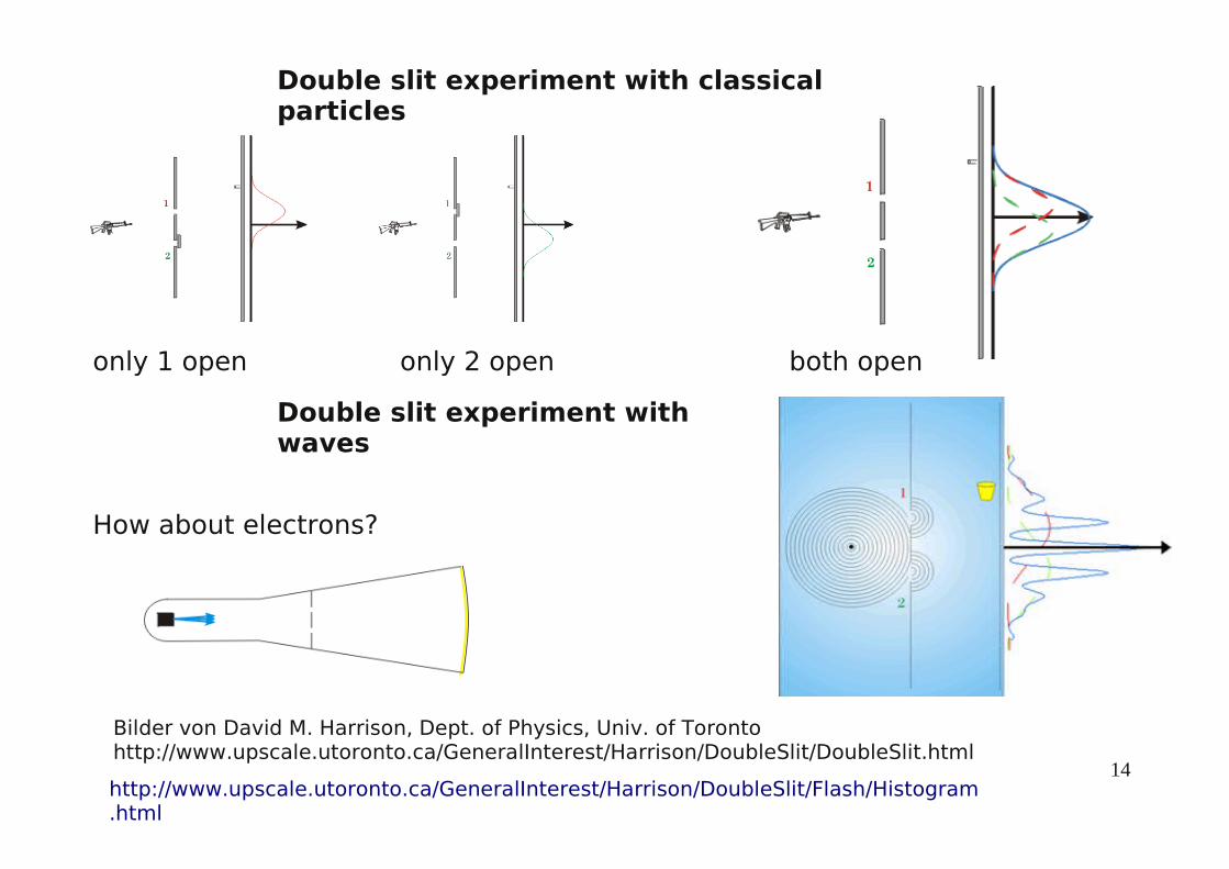
14http://www.upscale.utoronto.ca/GeneralInterest/Harrison/DoubleSlit/Flash/Histogram.html
Double slit experiment with classical particles
only 1 open only 2 open both open
Double slit experiment with waves
How about electrons?
Bilder von David M. Harrison, Dept. of Physics, Univ. of Toronto http://www.upscale.utoronto.ca/GeneralInterest/Harrison/DoubleSlit/DoubleSlit.html

15
Wave character of electrons
1927 Electron diffraction using a Ni-crystal (Davisson & Germer)1961 Double slit experiment with electrons Claus Jönsson, Tübingen, Zeitschrift für Physik 161, 454 (1961)
The Jönsson experiment has been selected in September 2002 by the journal 'Physics World' as the most beautiful experiment of all times. http://physicsweb.org/articles/world/15/9/2
Electrons show particle or wave properties similar to light.

16
"Wave-particle duality of C60" Markus Arndt et al., Nature 401, 680-682, 14.October 1999
Wave-particle dualism for molecules: C60

17
Based on the particle-wave duality we can describe the state of any physical systemwith help of a wavefunction ψ(r,t).The square |ψ(r,t)|2=ψ*ψ is the probability density to find a particle at location r at time t.
2. Wave equation for free particles2.1 Wavefunction
The wavefunction ψ(r,t) is a complex scalar, because there was no polarization foundIn contrast to electromagnetic waves.
The probability to find the particle at time t in a volume element d3r located at r is given by
w(r,t) d3r =|ψ(r,t)|2d3r=ψ*ψ d3r.
Probability density w(r,t) =|ψ(r,t)|2=ψ*ψ
A single particle has to be somewhere in a given volume, therefore: ∫w(r,t) d3r =∫|ψ(r,t)|2d3r=∫ψ*ψ d3r=1
Normalization: If the above condition is not fulfilled for ψ(r,t) then we can always normalize to 1, by:
r ,t =∣ r , t ∣2
∫∣ r ,t ∣2 d3r

18
Wavefunction ψ(r,t)
Probabilities are positive definite numbers. Only the square has a real physicalinterpretation. The wavefunction (also called probability amplitude) ψ(r,t) itselfcan not be measured and no real physical interpretation.
For many equal photons (bosons) the intensity is given by the square of the wavefunction resulting from the superposition of the single photons |ψ(r,t)|2 = large -> many photons |ψ(r,t)|2=0 no photons
One possible interpretation of the wavefunction of matter is a statistical interpretation.
A single measurement will always detect a single particle, however the distribution in space and time is given by the square of the wavefunction.
There is no certainty to find a particle at a given location and time, but only a probability.
If there are alternative possibilities which will result in the same result then therewill be interference phenomena observed in QM. If the experimental setup is changed, so that the alternate possibilities can not be realized, the interference will vanish too.

19
Goal: To find the equation which gives as solution the wavefunction for particles.
Schrödingers equation can not be derived directly from first principles.
Therefore we try to 'guess' Schrödingers equation based on the wave-particle duality in analogy to light waves.
Wave-particle duality well proofed experimentally All particles with constant momentum have a wavelength (de Broglie 1924) QM as a general theory should contain the macroscopic correct classical mechanic in certain limits (Hamilton-Jacobi theory)
Motivation Schrödingers equation

20
2.2 Light waves (classical electrodynamics)
Wave equation from the Maxwell equations in case of the electric field:
E r , t =1c2
∂2
∂ t 2E r , t = ∂
2
∂ x 2∂
2
∂ y2∂
2
∂ z2
Ansatz: plane wavesE r , t = E0e
i k⋅r− t
will be a solution if ω=c k Wave vector k points in the direction of motion.
e.g. k || x-Axis E(x, t)=E0 cos(k x -ωt)
Period τ : E(x,t+τ)=E(x,t) -> ωτ = 2π ω = 2π/τ = 2π v Wavelength λ: E(x+λ,t)=E(x,t) -> kλ = 2π k = 2π/λ ω=c k -> 2π v = c 2π/λ -> v λ = c
Interference: E will be added (super position), because Maxwell eq. are linear differential equations
Intensity: ~ Energy-current density (Poynting vector) ~ |Re E|2
∣Re E1Re E2∣2=∣Re E1∣
2∣Re E2∣22 Re E1⋅Re E2
Intensity can not be superposed!

21
Remark on theory of special relativity
ED is a relativistic theory (c= speed of light), so that a relativistic wave equationresults into quantum electrodynamics.E=mc2
E2 = m2c4 = p2 c2 + m0
2c4
Energy and mass increase with momentum (velocity).Transition to classical mechanics in case of small p (c>>|v|)
E=m02c4p2c2=m0c
21 p2c2
m02c 4~m0c
2112p2c2
m02c4 =m0c
212p2
m01x ~11
2x ...
Light m0=0 photons have no rest mass but momentum
-> E2 = p2 c2 E = |p|c p=|p|
E = hv = ћω = ћ c k = p c -> p= ћk ( p = ћk )
E = ћω Energy photonp = ћk momentum photon
Therefore any particle with fixedmomentum has a well definedwave length.
because k=|k|=2π/λ p= ћk = ћ 2π/λ = h / λ de Broglie 1924
22
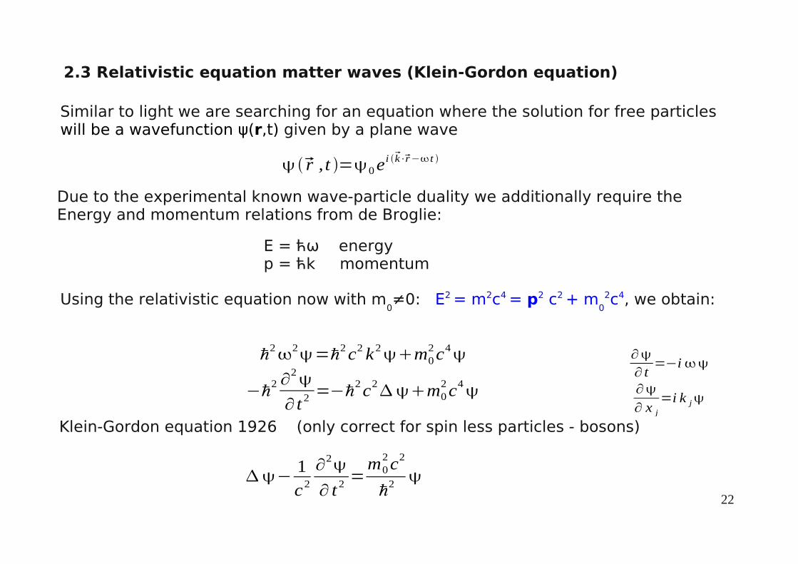
2.3 Relativistic equation matter waves (Klein-Gordon equation)
Similar to light we are searching for an equation where the solution for free particleswill be a wavefunction ψ(r,t) given by a plane wave
r ,t =0ei k⋅r− t
Due to the experimental known wave-particle duality we additionally require theEnergy and momentum relations from de Broglie:
E = ћω energyp = ћk momentum
Using the relativistic equation now with m0≠0: E2 = m2c4 = p2 c2 + m
02c4, we obtain:
ℏ22=ℏ2c2 k2m02c4
−ℏ2 ∂
2
∂ t 2 =−ℏ2c2m0
2c4
Klein-Gordon equation 1926 (only correct for spin less particles - bosons)
−1
c2
∂2
∂ t 2=m0
2c2
ℏ2
∂
∂ t=−i
∂
∂ x j
=i k j
23
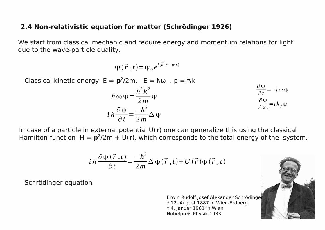
2.4 Non-relativistic equation for matter (Schrödinger 1926)
We start from classical mechanic and require energy and momentum relations for lightdue to the wave-particle duality.
r ,t =0ei k⋅r− t
Classical kinetic energy E = p2/2m, E = ћω , p = ћk
ℏ=ℏ
2k 2
2m
i ℏ∂
∂ t=−ℏ2
2m
∂
∂t=−i
∂
∂ x j
=i k j
In case of a particle in external potential U(r) one can generalize this using the classical Hamilton-function H = p2/2m + U(r), which corresponds to the total energy of the system.
i ℏ∂ r ,t ∂ t
=−ℏ
2
2mr ,t U r r , t
Schrödinger equation
Erwin Rudolf Josef Alexander Schrödinger * 12. August 1887 in Wien-Erdberg† 4. Januar 1961 in WienNobelpreis Physik 1933

24
Coherence length = Length of the wave
In reality wave have mo infinite extension like plane waves, but are rather given by Wave packets. Interference will only occur if the coherence length l
c is large
compared to the dimension of the measurement apparatus. e.g. realistic life times for radiation of a photon from an atom are about τ~10-8s. This corresponds to a coherence length l
c=c*τ ~ 3m of the wave packet.
2.5 Wave packets and coherence length
A Gauss wave packet is a wave modulated by a Gauss-function (Multiplication of the wavefunction by a Gauss-function).
ψ ψ*ψ

25
3. Wavefunction, Schrödinger equation and operators
The state of a QM system will be described by its wavefunctionψ(r,t)=wavefunction=state function
Probability density to find an electron at location r and time t is defined by the squareof wavefunktion.
w( r , t)=∣ψ( r , t)∣2
∫∣ψ( r , t)∣2 d3 r=
ψ*( r , t)ψ( r , t)
∫ψ*( r , t)ψ( r , t )d3 r
The wavefunction is the solution of the Schrödinger equation.
i ℏ∂ r ,t ∂ t
=H =−ℏ
2
2m r , t U r r ,t
H = Hamilton-operator (Operator: Function -> Function)Build from the Hamilton-function as defined in classical mechanics.

26
Example: free particle in large volume V
free = no acting forces -> potential energy U(r)=0Schrödinger equation:
i ℏ∂ r , t ∂ t
=H =−ℏ2
2m r , t
Solution will be plane waves:
ψ( r , t)=ψ0 ei( k⋅r−ωt ) with ℏω=
(ℏ k )2
2mi ℏ−i=
−ℏ2
2m− k 2
ℏ=ℏ2 k 2
2m
Normalization of the wavefunction
∫ *d3 r=∫0
*e−i k⋅r− t
0ei k⋅r− t d3 r=∫ 0
*0 d
3 r=0*0∫d3 r= 0
* 0V=1
∣0∣=1
VWe get a plane wave with fixed energy E = ћω and momentum p = ћk wave vector k || p and group velocity
v g k =d
dk=ℏ km=v
Where do we find the particle? |ψ(r,t)|2 = 1/VThe probability is equal in all points of space.

27
3.1 Operators and measurements
Momentum operator: classical momentum p will be replaced by QM operator pop
pop=ℏ
i ∂
∂ x,∂
∂ y,∂
∂ z =ℏ
igrad=
ℏ
i∇
pop2 = pop⋅ pop= ℏi ∇ ⋅
ℏ
i∇ =−ℏ2∇⋅∇=−ℏ2=−ℏ2 ∂
2
∂ x2∂2
∂ y2∂2
∂ z2 Position (space) operator: classical position r will be replaced by QM position operator r
op
r -> rop
= just multiplication with value r
Function depending on coordinates U(r) -> Uop
(r) multiplication with value of function
Index op will not be used further!
The order of operators can not be permuted in the general case!
x p x r , t =x p x r , t =x ℏi∂ r , t ∂ x
p x x r , t = p x x r , t = ℏi ∂∂ x x r , t =ℏ
i r , t x∂ r , t ∂ x
x p x− p x x r , t =−ℏ
ir , t

28
Eigenvalues of operators correspond to physical values of measurements.
A) momentum measurement for plane waves:
Eigenvalue equation from linear algebra
a11 a12
a21 a22 x1
x2= x1
x2 A x= x
pop=ℏ
igrad=p p=ℏk nach de Broglie
r ,t =0ei k⋅r− t
QM: Operator function = Number function
B) Hamilton operator free particle
H op=−ℏ2
2m=
pop2
2m
H op=pop
2
2m=
ℏ2 k 2
2m=E
Eigenvalues of the Hamilton operator are just possible values of the energy.
C) general case: Operator A corresponds to a certain physical measurement
Eigenvalue equation A ψ=aψ
Eigenvaluea=possible value of measurement
29
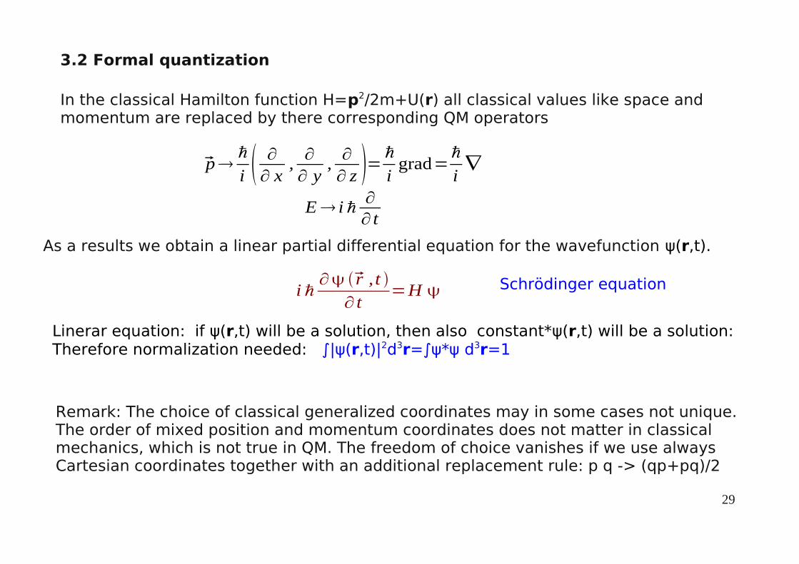
In the classical Hamilton function H=p2/2m+U(r) all classical values like space and momentum are replaced by there corresponding QM operators
3.2 Formal quantization
pℏ
i ∂
∂ x,∂
∂ y,∂
∂ z =ℏ
igrad=
ℏ
i∇
E i ℏ∂∂ t
As a results we obtain a linear partial differential equation for the wavefunction ψ(r,t).
i ℏ∂ r ,t ∂ t
=H
Linerar equation: if ψ(r,t) will be a solution, then also constant*ψ(r,t) will be a solution:Therefore normalization needed: ∫|ψ(r,t)|2d3r=∫ψ*ψ d3r=1
Remark: The choice of classical generalized coordinates may in some cases not unique.The order of mixed position and momentum coordinates does not matter in classicalmechanics, which is not true in QM. The freedom of choice vanishes if we use alwaysCartesian coordinates together with an additional replacement rule: p q -> (qp+pq)/2
Schrödinger equation

30
3.3 Stationary (time independent) states
In case of an Hamilton operator which does not depend on time, it is possible to derive from the full time-dependent Schrödinger equation a stationary Schrödinger equation.
iℏ∂ψ( r , t)∂ t
=H ψ=−ℏ
2
2mΔ ψ( r , t)+ U ( r )ψ( r , t)
Ansatz: Separation of variables ψ( r , t)=f (t )ϕ( r )
iℏϕ( r )∂ f (t )∂ t
=H f (t)ϕ( r )
Dividing by ψ(r,t) one obtains the stationary Schrödinger equation H Φ(r) = E Φ(r). The solution Φ(r) are called stationary states which have fixed energy.The time part equals to f(t)=e-iωt with E = ћω.
w( r , t)=ψ*( r , t )ψ( r , t)=eiω tϕ*
( r )e−iω tϕ( r )=ϕ*( r )ϕ( r )=w( r )
The probability density is time independent, even if the wavefunction is stilltime dependent ψ(r,t) = e-iωt Φ(r)
31
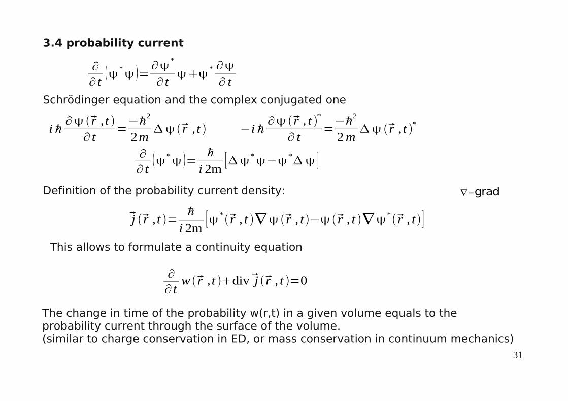
3.4 probability current
∂
∂ t* =
∂*
∂ t
* ∂
∂ t
i ℏ∂ r ,t ∂ t
=−ℏ
2
2mr ,t −i ℏ
∂ r , t *
∂ t=−ℏ
2
2m r ,t *
Schrödinger equation and the complex conjugated one
∂
∂ t* =
ℏ
i 2m[*−* ]
Definition of the probability current density:
j r ,t =ℏ
i 2m[*r , t ∇ r , t − r , t ∇*r , t ]
This allows to formulate a continuity equation
∂∂ t
w r ,t divj r , t =0
The change in time of the probability w(r,t) in a given volume equals to theprobability current through the surface of the volume.(similar to charge conservation in ED, or mass conservation in continuum mechanics)
∇=grad
32
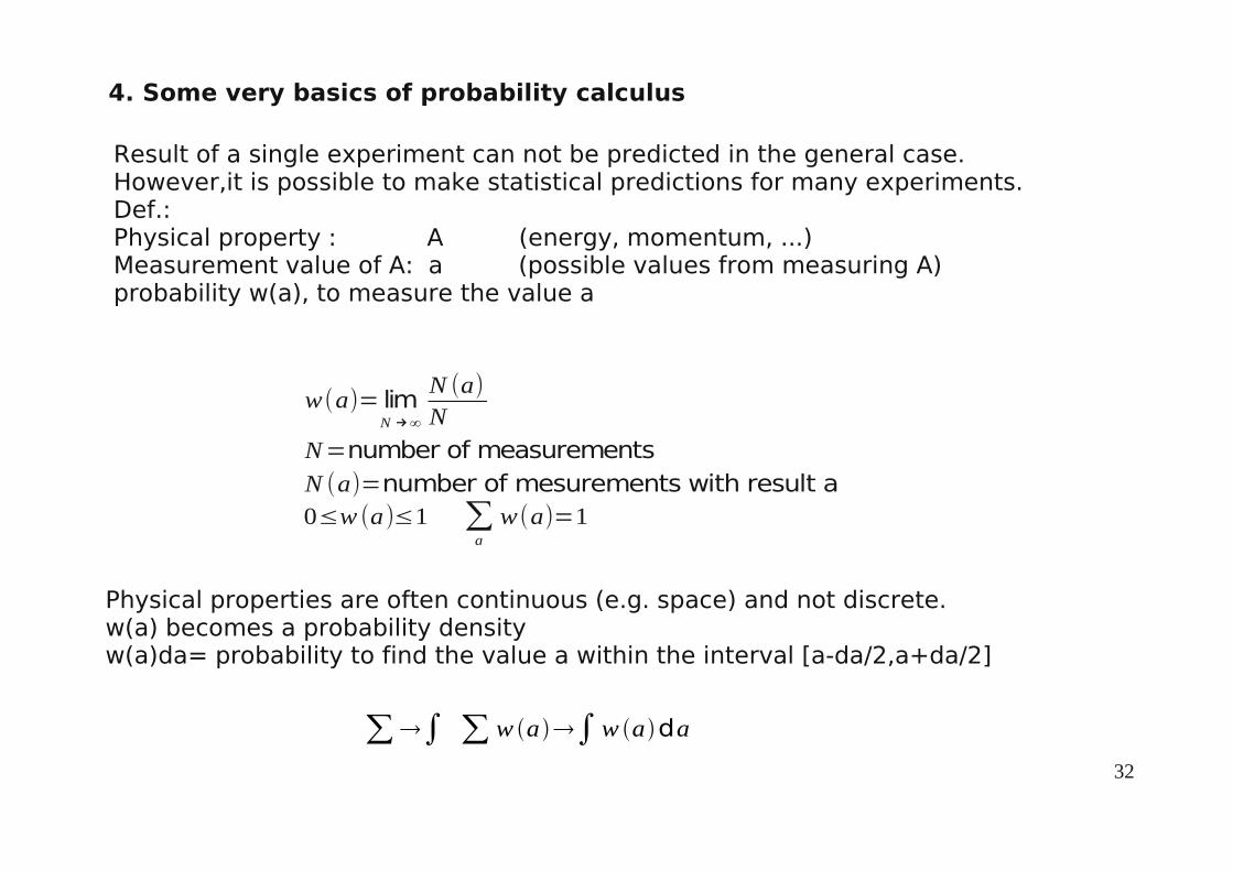
4. Some very basics of probability calculus
Result of a single experiment can not be predicted in the general case.However,it is possible to make statistical predictions for many experiments.Def.:Physical property : A (energy, momentum, ...)Measurement value of A: a (possible values from measuring A)probability w(a), to measure the value a
w(a)= limN →∞
N (a)N
N=number of measurementsN (a)=number of mesurements with result a0≤w (a)≤1 ∑
a
w(a)=1
Physical properties are often continuous (e.g. space) and not discrete.w(a) becomes a probability densityw(a)da= probability to find the value a within the interval [a-da/2,a+da/2]
∑∫ ∑ w a∫w ada

33
Average of the property A is also called expectation value
⟨ A ⟩=A=∑a
aw a
4.1 Averages (expectation values)
Average of a function f(A)
⟨ f A⟩=∑a
f a w a ⟨ f A ⟩=∫a
f a w a da
Which experiment is more accurate?
0 2 4 6 8 10 120
0,5
1
1,5
2
2,5
Messungen
0 2 4 6 8 10 121,41,51,61,71,81,9
22,12,22,3
Messungen
34
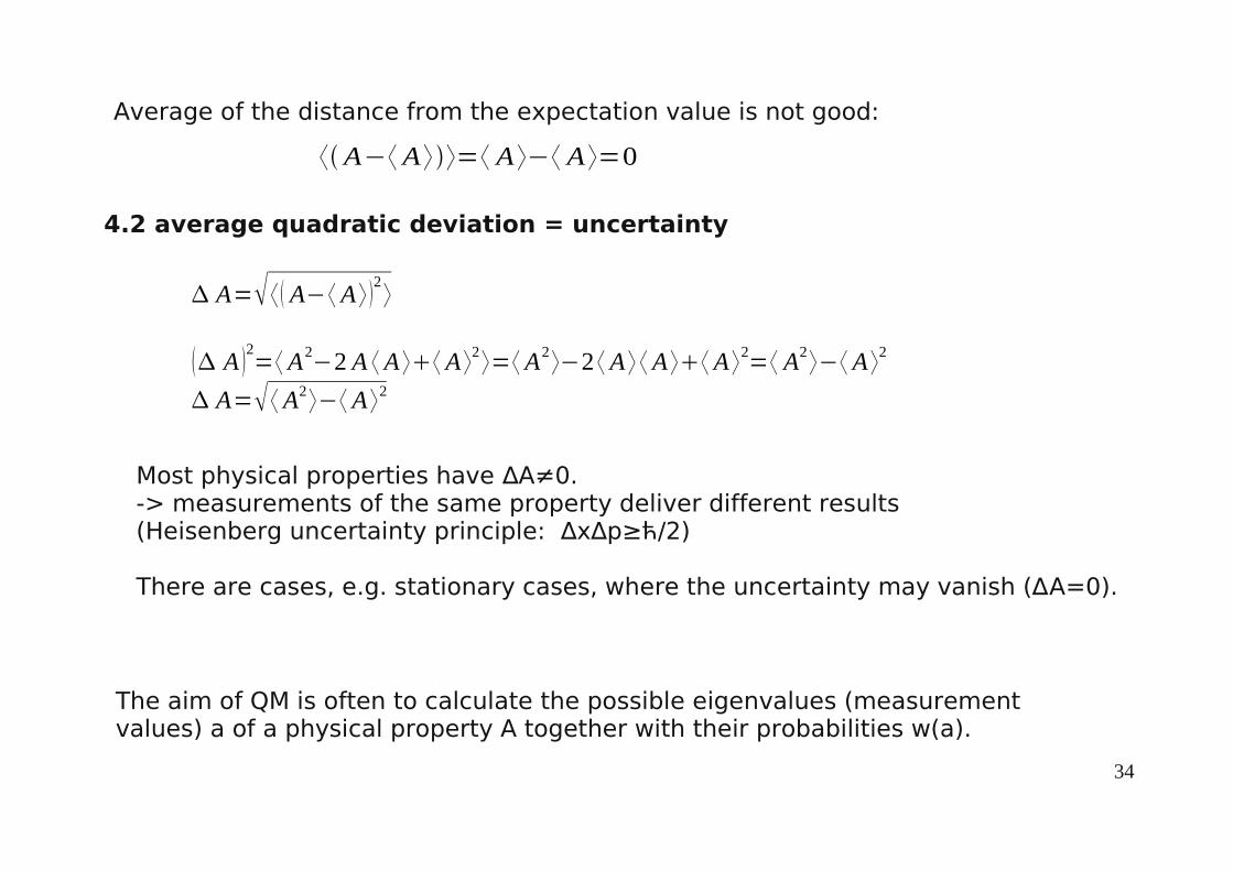
4.2 average quadratic deviation = uncertainty
Average of the distance from the expectation value is not good:
⟨A−⟨ A⟩⟩=⟨ A ⟩−⟨ A ⟩=0
A= ⟨ A−⟨ A ⟩ 2⟩
A 2=⟨ A2
−2 A ⟨ A ⟩⟨ A ⟩2⟩=⟨ A2⟩−2 ⟨ A ⟩ ⟨ A ⟩⟨ A ⟩2=⟨ A2
⟩−⟨ A ⟩2
A= ⟨ A2⟩−⟨ A ⟩2
Most physical properties have ∆A≠0.-> measurements of the same property deliver different results(Heisenberg uncertainty principle: ∆x∆p≥ћ/2)
There are cases, e.g. stationary cases, where the uncertainty may vanish (∆A=0).
The aim of QM is often to calculate the possible eigenvalues (measurement values) a of a physical property A together with their probabilities w(a).
35
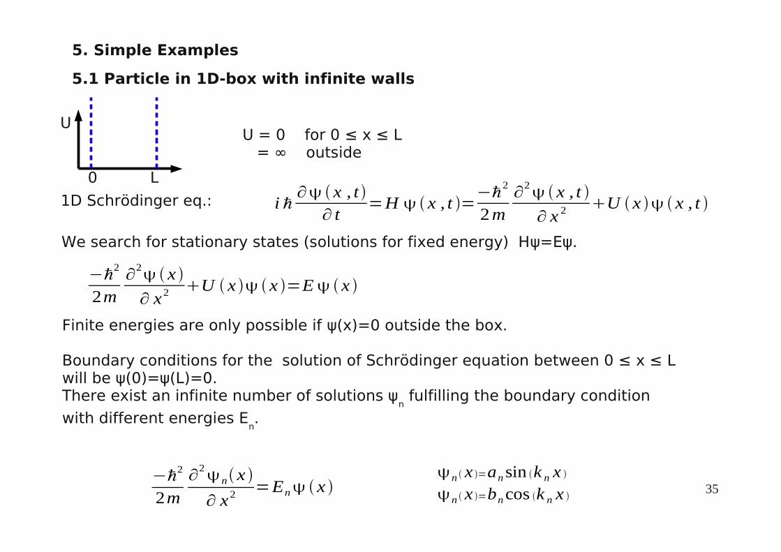
5. Simple Examples
5.1 Particle in 1D-box with infinite walls
0 L
UU = 0 for 0 ≤ x ≤ L = ∞ outside
i ℏ∂ x , t ∂ t
=H x , t =−ℏ
2
2m∂
2 x , t
∂ x 2 U x x , t 1D Schrödinger eq.:
We search for stationary states (solutions for fixed energy) Hψ=Eψ.
−ℏ2
2m∂
2 x
∂ x2 U x x =E x
Finite energies are only possible if ψ(x)=0 outside the box.
Boundary conditions for the solution of Schrödinger equation between 0 ≤ x ≤ L will be ψ(0)=ψ(L)=0.There exist an infinite number of solutions ψ
n fulfilling the boundary condition
with different energies En.
−ℏ2
2m∂
2n x
∂ x2=En x
n x =ansin k n x n x =bncos k n x
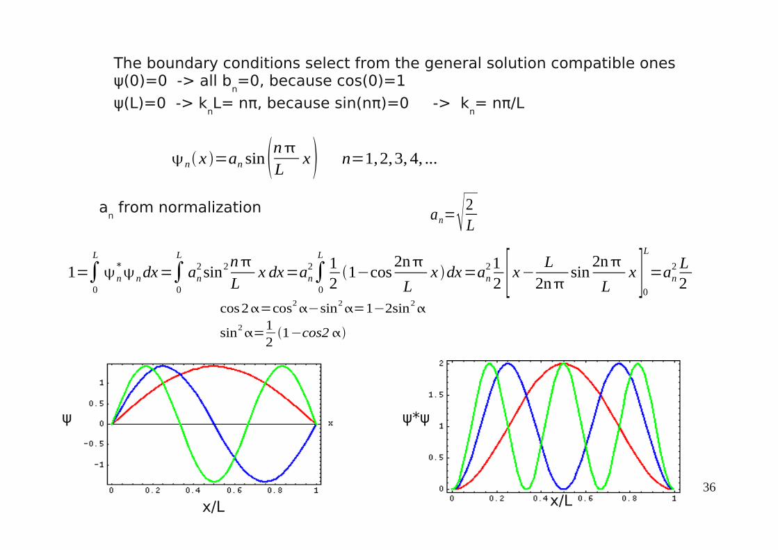
36
The boundary conditions select from the general solution compatible onesψ(0)=0 -> all b
n=0, because cos(0)=1
ψ(L)=0 -> knL= nπ, because sin(nπ)=0 -> k
n= nπ/L
n x =an sin nL x n=1,2,3, 4, ...
an from normalization
1=∫0
L
n*ndx=∫
0
L
an2 sin2n
Lx dx=an
2∫0
L121−cos
2n
Lx dx=an
2 12 [ x− L
2nsin
2n
Lx ]
0
L
=an2 L2
cos2=cos2−sin2
=1−2sin2
sin2=
121−cos2
an=2L
x/L x/L
ψ ψ*ψ
37
Distance between two energy levels
En1−E n=ℏ
2
2m
2
L2n12−n2=ℏ
2
2m
2
L22n1
L large: very small energy differences, practical energies appear continuousL small: only discrete energy differences allowed (-> sharp spectral lines)
En x =−ℏ
2
2m
∂2n x
∂ x2 =ℏ
2
2m nL
2
ansin nL x En=
ℏ2
2m nL
2
=ℏ2k n
2
2m
Energies can be obtained from putting ψn(x) in the Schrödinger equation:
Due to the boundary condition not all energies are allowed anymore.The discrete energy levels correspond to the measurable energy eigenvalues of the system. This is a qualitatively new results of QM.
The uncertainty of the energy is the state ψn vanishes ∆E
n=0.
An=ann
A2n=A An=A an=an2n

38
En1−E n=ℏ
2
2m
2
L2n12−n2=ℏ
2
2m
2
L22n1
E = hv = ћω = ћ c k = h c /λ
Absorption spectra of aromatic moleculesShow with increasing molecular size ashift to larger wave length(smaller energies).
Electrons in π-bonds are only weakly bondedand can be approximately described by particles in a box of a length given by thesize of the molecule.
Absorptions spectra of aromatic ring molecules
Haken&Wolf, Molekülphysik und Quantenchemie, S.259

39
5.2 Particle in 3D-box with infinite walls
L1
L2
L3
−ℏ2
2m ∂2
∂ x2∂2
∂ y2∂2
∂ z2 x , y , z =E x , y , z
Similar boundary condition as before:
0, y , z = L1, y , z =0 x ,0 , z = x , L2, z =0 x , y ,0= x , y , L3=0
Ansatz: Separation of variables ψ(x,y,z)= ψ(x) ψ(y) ψ(z)
n1n2n3 x , y , z =2
L1
sin n1
L1
x 2L2
sin n2
L2
y2L3
sin n3
L3
z E n1n2n3
=ℏ2
2m
2n12
L12
n22
L22
n32
L32
Sommerfeld model of metals: explanation of electric conductivity using QM

40
5.3 Tunnel effect
U0
U0
kinetic energy smaller than U0
kinetic energy larger than U0
classical MechanicReflexion, Scattering
QM: What are the states with fixed energy?
I II III
0 L
I : −ℏ2
2md 2
dx 21 x =E1 x 1 x =A1e
i k 1 xB1e−i k 1 x E=
ℏ2
2mk 1
2
I I : −ℏ2
2md 2
dx 2 2x U 0 2 x =E2 x 2 x =A2ei k 2 xB2e
−i k 2x E=ℏ2
2mk 2
2U 0
I I I : −ℏ
2
2md2
dx23 x =E 3 x 3 x =A3 e
i k 3 xB3e−i k 3 x E=
ℏ2
2mk 3
2
(general solution for 2. order differential eq. -> see Mathematics)
Energy given and constant in all parts (energy conservation)
k 1=k 3=1ℏ2m E k 2=
1ℏ2m E−U 0
k2 for E<U
0 imaginary k
2=iκ

41
5.3 Tunnel effect
U0
U0
kinetic energy smaller than U0
kinetic energy larger than U0
classical MechanicReflexion, Scattering
QM: What are the states with fixed energy?
I II III
0 L
I : −ℏ2
2md 2
dx 21 x =E1 x 1 x =A1e
i k 1 xB1e−i k 1 x E=
ℏ2
2mk 1
2
I I : −ℏ2
2md 2
dx 2 2x U 0 2 x =E2 x 2 x =A2ei k 2 xB2e
−i k 2x E=ℏ2
2mk 2
2U 0
I I I : −ℏ
2
2md2
dx23 x =E 3 x 3 x =A3 e
i k 3 xB3e−i k 3 x E=
ℏ2
2mk 3
2
(general solution for 2. order differential eq. -> see Mathematics)
Energy given and constant in all parts (energy conservation)
k 1=k 3=1ℏ2m E k 2=
1ℏ2m E−U 0
k2 for E<U
0 imaginary k
2=iκ

42
Boundary condition: wavefunction should be continuous
1 0= 2 0dd x 1 0 =
dd x 2 0
2 L = 3 L dd x 2 L =
dd x 3 L
I II III
0 L
4 equations but 6 unknowns, one additional condition due to normalization-> one of the unknowns is not determined -> use experimental setup to define onee.g. particles come only from part I but not from III → B
3=0 (no back scattering in III)
I II III
0 L
A3 corresponds to classical forbidden contribution
Using the conditions together with the general solution we obtain a linear system of equations to solve for the unknown constants.
A1B1=A2B2 A1k 1−B1k 1=A2k 2−B2k 2
A2ei k 2 L
B2e−i k 2 L
=A3ei k 1 L A2k 2e
i k 2 L−B2k 2e
−i k 2 L=A3 k 1e
i k 1 L
43
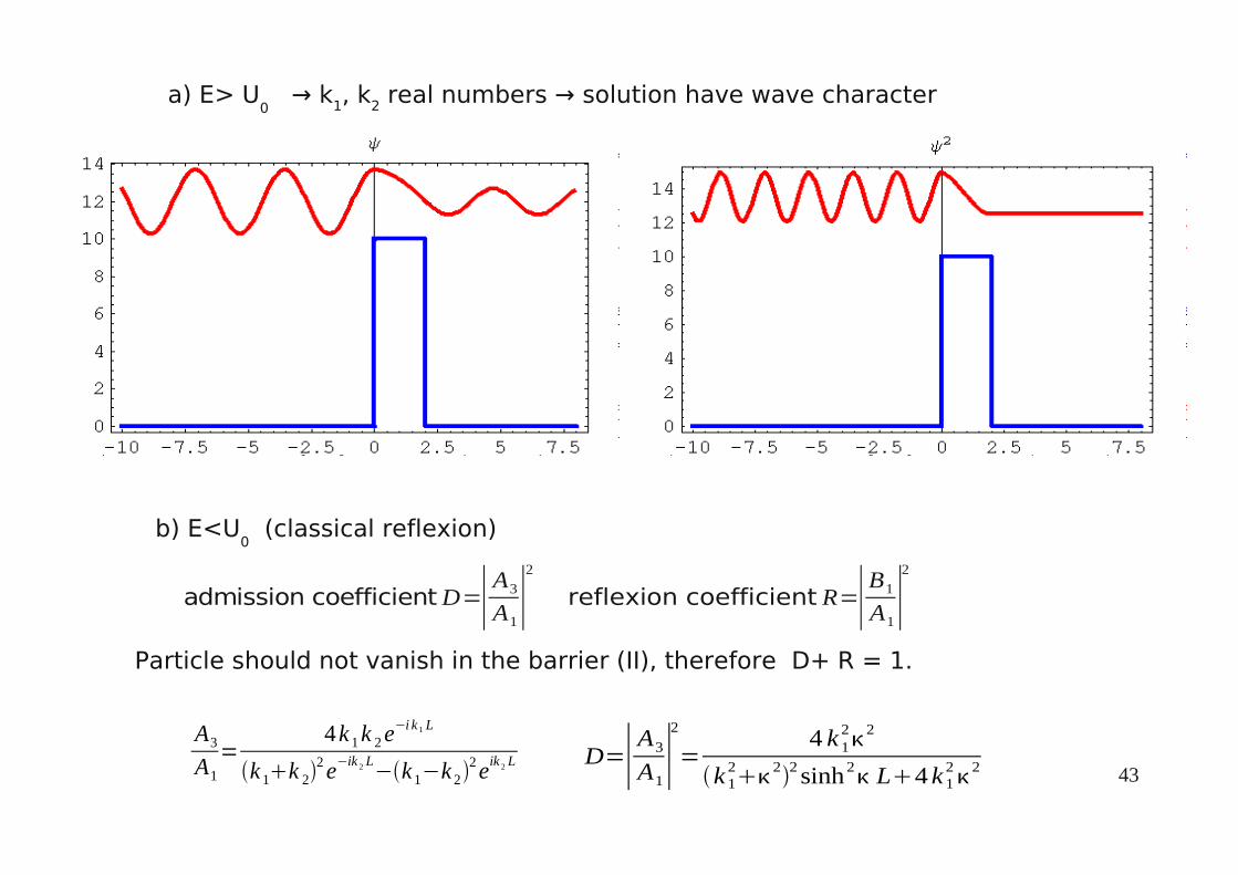
b) E<U0 (classical reflexion)
admission coefficientD=∣A3
A1∣2
reflexion coefficient R=∣B1
A1∣2
Particle should not vanish in the barrier (II), therefore D+ R = 1.
A3
A1
=4k 1k 2e
−i k 1 L
k 1k 22e−ik 2 L−k 1−k 2
2eik 2 L D=∣A3
A1∣2
=4 k 1
22
k 12
22 sinh2
L4k 12
2
a) E> U0 → k1, k2 real numbers → solution have wave character

44
k 1=k 3=1ℏ2m E =
1ℏ2m U 0−E
sinh L=12e L−e− L ≈ 1
2eL falls L≫1 sinh 2
L≈14e2 L
D=∣A3
A1∣2
=4 k 1
2
2
k 12
22 sinh2
L4k 12
2 ≈16k 1
2
2
k 12
22 e
−2 L
Typical for solids (metals) U0-E~5eV,
In case of electron :L=1Å : e-2κL ~ 0.1L=2Å : e-2κL ~ 0.01L=10Å : e-2κL ~ 10-10
The admission decreases exponentially with the width L of the barrier.The bigger the mass the smaller is theadmission coefficient D.

45
Is the tunnel effect important?
Qualitative understanding of the chemical bondDue to the tunneling process the total energy of the system can be lowered -> this is one reason for binding energies
benzen: Collective tunneling of all double bonds -> all C-C bonds have the same length
Radioactive α-decay
α-particles are able to tunnel out of the nuclear box1/r
46
6. Hilbert space and linear operators (mathematical foundation QM)
6.1 Hilbert space
space = mathematical construct: vector space
a) The linear complex space is the set of mathematical objects having the followingproperties
1. ψ and φ are elements of the set, then ψ±φ is also an element of the set.2. It exist one element 0 (zero element) with ψ+0=ψ, ψ-ψ=0.3. If ψ is an element of the set, the is λψ (λ= complex number) also element of the set.
David Hilbert * 23. Januar 1862 Königsberg† 14. Februar 1943 Göttingen

47
Examples:
I. Set of complex 3D vectors a=(ax,a
y,a
z) with a
x=Re a
x + i Im a
x
a, b are vectors, then is a±b=(ax±b
x,a
y±b
y,a
z±b
z) also a vector
a + (0,0,0)=a zero vector (0,0,0) λa=(λa
x,λa
y,λa
z) is a vector λa
x = Multiplication of two complex numbers
II. Set of all wavefunction (state functions) which are solution of Schrödinger equation ψ(r,t) and φ(r,t) are solutions of Schrödinger equation, then is ψ±φ also a solution function identical zero is solution of Schrödinger equation λψ(r,t) is also a solution
III. other mathematical sets (e.g. matrices)

48
The Hilbert space is a linear complex space, which has defined additionally a scalar product with the following properties:0. (ψ,φ) = a = complex number (Mathematics: a is finite)1. (ψ, λφ) = λ(ψ,φ) λ = complex number2. (φ,ψ) = (ψ,φ)* = a*
=> (λψ,φ) = (φ,λψ)* = [λ(φ,ψ)]* = λ*(φ,ψ)* = λ*(ψ,φ)
(ψ,φ1±φ
2) = (ψ,φ
1) ± (ψ,φ
2)
=> (ψ1±ψ
2,φ) = (ψ
1,φ) ± (ψ
2,φ)
(ψ,ψ) ≥ 0 and real, finite (ψ,ψ) = 0 only if ψ = 0
Def. Norm („length“):
ψ, φ are orthonormal, if
b) Hilbert space of physicists
,=∥∥
,= 0 ≠
1 =

49
c) Hilbert space (mathematicians)
Additional requirement of completeness Very important for mathematicians but any complex vector space can be completed
e.g., Completing rationale numbers by irrational numbers → limits have to be elements of the space
e.g. set of all real polynomials of order N,form a linear space, scalar product defined as
then
sin = limit of the polynomials for N -> ∞
Mathematical correct definition of the Hilbert space:A linear complex space which is complete with respect to the metric induced by thescalar product, this means that all Cauchy series will converge, is called Hilbert space.
f N x =∑n=0
N
an xn
f N , f M ≝∫0
2
f n⋅ f m dx
sin x=x−x3
3 !x5
5 ! ⋯ =∑
n=0
∞
an xn
50
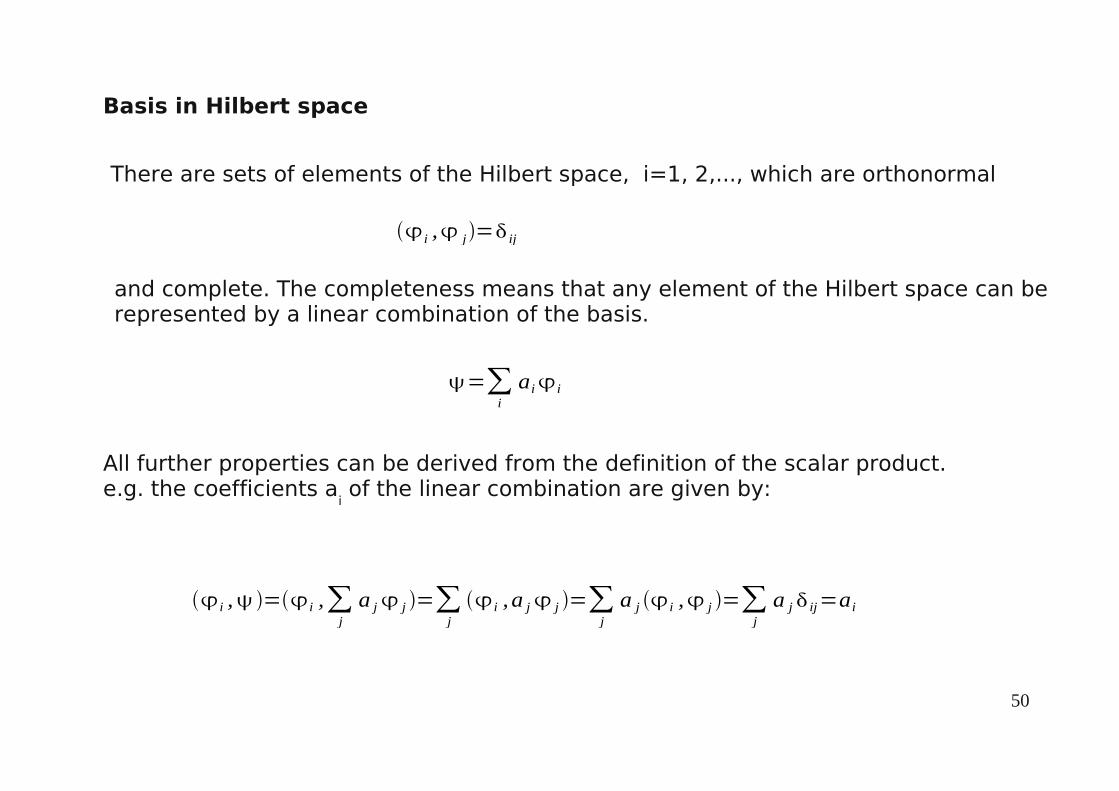
Basis in Hilbert space
There are sets of elements of the Hilbert space, i=1, 2,..., which are orthonormal
and complete. The completeness means that any element of the Hilbert space can berepresented by a linear combination of the basis.
i , j= ij
=∑i
aii
All further properties can be derived from the definition of the scalar product.e.g. the coefficients a
i of the linear combination are given by:
i ,= i ,∑j
a j j =∑j
i , a j j =∑j
a j i , j =∑j
a j ij=ai

51
Examples
complex vectors
real vector
a ,b=a x* bxa y
* b yaz* bz ∥a∥=∣ax∣
2∣a y∣2∣az∣
2
,=⟨∣⟩=∫*r ,t r , t d 3r
The solutions of Schrödingers equation (wavefunctions)are elements of a Hilbert space with a scalar product defined as:
,=∫* d3
r=∫ *
*d 3r= ,*
,=∫*d 3
r=∫ *d 3
r
,=∫ *d 3r=∫**d 3
r=*∫*d 3r
,1±2=∫*1±2d
3r=∫ *
1d3r±∫*
2 d3r= ,1± ,2
Dirac notation for the scalar product <ψ|φ>bra = <ψ| ket=|φ>
Paul Adrien Maurice Dirac * 8. August 1902 Bristol † 20. Oktober 1984 TallahasseeNobelpreis Physik 1933

52
Comparison N-dimensional vektor space with Hilbert space
Vector space Hilbert space a Vector ψ e
n Basis φ
n
ei·e
j=δ
ij Orthogonality <φ
i |
φ
j> = δ
ij
a = ∑ ai e
i linear combination ψ=∑ a
i φ
i
a
i = e
i·a a
i = <φ
i |
ψ>
a·b = b·a Symmetry scalar product <φ | ψ> = <
ψ | φ>*
The elements of the Hilbert space in QM are normalizable functions, the dimension ofHilbert space is infinite. The basis is given by a suitable, complete and orthonormal setof functions.

53
1. Schwarz inequality
(real vectors = length of vector)
2. triangle inequality
real vectors = Length a
∣ ,∣∥∥∥∥= , ,
∥a∥=ax2a y2a z
2
∣a⋅b∣=∣a⋅b⋅cos∣a⋅b ∣cos∣≤1
∥∥∥∥∥∥
∥a∥ab
a
b
6.2. Mathematical properties
b
a
54
1. Schwarz inequality
(real vectors = length of vector)
2. triangle inequality
real vectors = Length a
∣ ,∣∥∥∥∥= , ,
∥a∥=ax2a y2a z
2
∣a⋅b∣=∣a⋅b⋅cos∣a⋅b ∣cos∣≤1
∥∥∥∥∥∥
∥a∥ab
a
b
6.2. Mathematical properties
b
a

55
6.3. Linear operators in Hilbert space
Def: An operator maps an element of the Hilbert space on another element.
Matrix in the space of 3D vectors
Translation operator
Operator must not known explicit, knowing its result is sufficient!
Inversion operator
Einstein: Summation overdouble index (Einsteinsum convention)
A=
a xx a xy a xz
a yx a yy a yz
a zx a zy a zzbxb y
b z=
c xc ycz
aijb j=cix1, y2, z3
∑j=1
3
aijb j=ci
∂∂ x=
T x , y , z = xa , yb , zc
P r = −r

56
Def: Operator A is linear if:
Example for nonlinear operator: Multiplication with
In general e.g. A = px, B = x
Def: The combination of two operators A and B in the following way: AB – BA =[A,B] = C (another operator) is called Commutator.
A 1122=1 A12 A2
A= ,A = ,
∥∥2
AB≠B A
[ x , px]=i ℏ[ x , py ]=0
[ x , x ]=0 [ p x , p x]=0
57
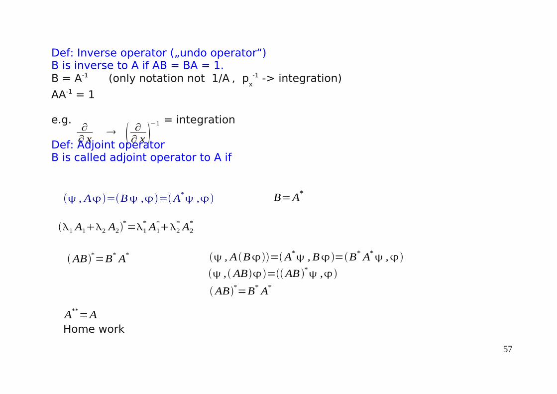
Def: Inverse operator („undo operator“)B is inverse to A if AB = BA = 1.B = A-1 (only notation not 1/A
, p
x
-1 -> integration)
AA-1 = 1
e.g. = integration
Def: Adjoint operatorB is called adjoint operator to A if
∂∂ x
∂∂ x −1
, A=B ,=A* ,
1 A12 A2*=1
* A1*2
* A2*
AB*=B* A*
B=A*
, A B=A* , B=B* A*
,
, AB=AB * ,
AB*=B* A*
A**=A
Home work

58
Def: self-adjoint (hermitian) Operator Operator A is called self-adjoint if A* = A. All physical meaningful operators are hermitian (self-adjoint).
Def: Unitary OperatorDef: Operator U is called unitary if U* = U-1
UU* = U*U = 1The scalar product is invariant under any unitary transformation.
(Uψ,Uφ) = (ψ,φ) (U*Uψ,φ) = (ψ,φ)
Example: Translation operator Tψ(x) = ψ(x+a) location x shifted by constant a
,=∫−∞
∞
dx*x x
T , T =∫−∞
∞
dx*xa xa
=∫−∞
∞
dy* y y
y=xa
dy=dx

59
Fourier-transformation F[ψ(x)] = ψ(k)(Fφ,Fψ) = (φ,ψ) Norm does not change Examples for hermitian operators:
1)
position operator x is hermitian Operator (y, z similar)-> r is hermitian operator
2)
, x=∫ d3r *
r xr
=∫ d 3r xr *r
= x ,
⟨∣p x⟩= ,ℏ
i∂∂ x=∫ d 3
r *r ℏ
i∂∂ xr =
partial integration
∫dx f x ddx
g x =
= f x g x∣ −∫dx ddx f x g x
0, in case ψ* and/or φ vanish at ∞
=∫d 3r ℏi ∂∂ x r
*
r = ℏi ∂∂ x ,=⟨ p x∣⟩
=∫dy dz* x , y , z x , y , z ∣x=−∞x=∞ −∫d 3r ℏi ∂∂ x * r r

60
px=ℏ
i∂∂ x
Is a hermitian operator (py,p
z similar)
p=ℏ
igrad is hermitian operator
Remarkψ, φ are plane waves, e. g. r =ei
k 1⋅r r =eik 2⋅r
≠0 for r∞
,ℏ
i∂∂ x=∫ d 3
r e−ik1⋅r ℏ
i∂∂ x
eik 2⋅r
=∫d 3r e−i
k 1⋅r ℏ
ii k 2
x e ik 2⋅r
=ℏ k 2x ∫ d 3
r e−i k 1− k 2⋅r
=ℏ k 2x23 3
k 1−k 2

61
ℏi ∂∂ x ,=∫ d 3r ℏi ∂∂ x e ik1⋅r
*
e ik 2⋅r
=∫ d 3r ℏ k 1
x eik 1⋅r
*
eik 2⋅r
=ℏ k 1x∫ d 3
r e−ik 1⋅r e i
k 2⋅r=ℏ k 1x∫ d 3
r e−i k 1−k 2⋅r
=ℏ k 2x 233 k 1−k 2
0 for ≠0 for
3k−k ' =
k 1≠ k 2
k 1= k 2
, px = p x , px is hermitian
-> is hermitianp
Similar proof for py and p
z, therefore if all components of the momentum operator
are hermitian then
62
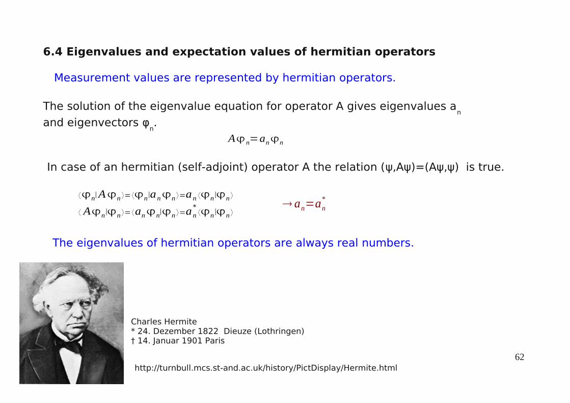
Measurement values are represented by hermitian operators.
A n=ann
6.4 Eigenvalues and expectation values of hermitian operators
http://turnbull.mcs.st-and.ac.uk/history/PictDisplay/Hermite.html
Charles Hermite * 24. Dezember 1822 Dieuze (Lothringen)† 14. Januar 1901 Paris
The solution of the eigenvalue equation for operator A gives eigenvalues an
and eigenvectors φn.
In case of an hermitian (self-adjoint) operator A the relation (ψ,Aψ)=(Aψ,ψ) is true.
⟨n∣An ⟩=⟨n
∣ann ⟩=an ⟨n∣n ⟩
⟨ An∣n ⟩=⟨ann
∣n ⟩=an*⟨n
∣n ⟩ an=an
*
The eigenvalues of hermitian operators are always real numbers.

63
The eigenvectors of hermitian operators form a basis in Hilbert space.
⟨m∣An⟩=⟨m∣ann ⟩=an ⟨m∣n⟩
⟨ Am∣n⟩=⟨amm∣n⟩=am* ⟨m∣n ⟩=am ⟨m∣n⟩
The difference of both equations in case of hermitian operators gives:
0=an−am ⟨m∣n⟩
Therefore, in case of different eigenvalues an≠a
m, the corresponding eigenfunctions
have to be orthogonal (scalar product is zero).
If one eigenvalue has several eigenfunctions (degeneracy), it is always possibleto build linear combinations of these eigenfunctions which are orthogonal(Gram-Schmidtsch orthogonalisation).
By means of normalization of the eigenfunctions we obtain an orthonormal basis in Hilbert space, so that any state can be expressed as a linear combination in that basis.

64
6.5 Expectation values of hermitian operators
An=ann
Assume we know for an hermitian operator A the eigenvalues and eigenfunctions.
Then we can represent any state of a physical system by a linear combination using thebasis given by the eigenfunctions of A.
=∑icii=∑
ici ∣i ⟩
The expectation value to measure the physical property A in such state will be:
⟨ A⟩= , A =⟨∣A ⟩=⟨∣A∑icii ⟩=∑
ic i ⟨∣A i ⟩=∑
ic i ⟨∣ai i ⟩=∑
ic iai ⟨∣ i ⟩=
=∑iaic i ⟨∑
jc j j∣ i ⟩=∑
i∑jc j
*aic i ⟨ j∣ i ⟩=∑
i∑jc j
*ai c i ij=∑iai c i
*c i=∑iai∣c i∣
2
That means we will measure the value ai with probability |c
i|2.

65
All physical properties can be represented by an hermitian (self-adjoint) operator.
The eigenvalues of such operators are always real numbers and correspond to the possible measurement values of the physical property.
The eigenfunctions of any hermitian operator can be used as basis in the Hilbert space, so that any state can be expressed as linear combination of these basis states.
The measurement of a physical property in a state ψ delivers always an eigenvalue with probability |c
i|2. The probability is given by the contribution of the corresponding
basis function to the state ψ.
If the system under investigation is already in an eigenstate, then we will always measure the same eigenvalue corresponding to the eigenstate without uncertainty.
6.6 Hermitian operators and measurement

66
7. Heisenberg uncertainty principleA*=A, B*=B are 2 hermitian linear operators (= physical properties)
1)
Because for any complex number z holds:
2) Schwarz inequality
Square of the equation
ψ, φ are arbitrary vectors, so that we replace these by new ones
Using the hermitian properties and 1) we obtain
∣A , B∣ ≥12∣A , B−A , B*∣ =
12∣A , B−B , A∣
=12∣ ,[A , B ] ∣
=12∣ , AB− , B A∣
∣z∣=Re z 2Im z2 ≥12∣z−z*
∣ =12∣2 i Im z∣ = ∣Im z∣
∥∥ ∥∥ ≥ ∣ ,∣ ∥∥ = ,
, , ≥ ∣ ,∣2
A , B
A , AB , B ≥ ∣A , B∣2
, A2 , B2 ≥14∣ ,[ A , B ] ∣2
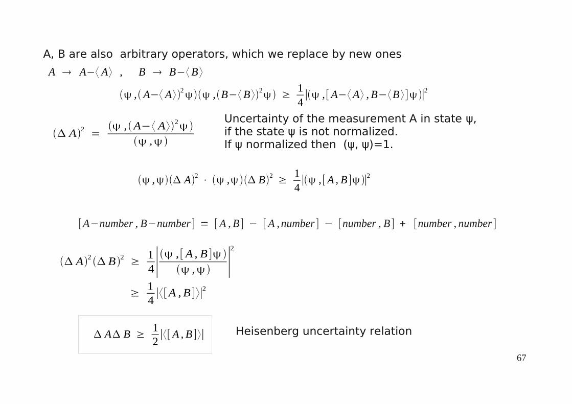
67
A, B are also arbitrary operators, which we replace by new ones
A A−⟨ A⟩ , B B−⟨B ⟩
A2 = ,A−⟨ A⟩2
,
, A2 ⋅ , B2 ≥14∣ , [ A , B ] ∣2
[A−number , B−number ] = [A , B ] − [A ,number ] − [number , B ] + [number , number ]
A2 B 2 ≥14∣ , [A , B ]
, ∣2
≥14∣⟨[A , B ]⟩∣2
A B ≥12∣⟨[A , B ]⟩∣ Heisenberg uncertainty relation
, A−⟨ A⟩2 ,B−⟨B⟩2 ≥14∣ ,[A−⟨A⟩ , B−⟨B⟩] ∣2
Uncertainty of the measurement A in state ψ, if the state ψ is not normalized. If ψ normalized then (ψ, ψ)=1.

68
A B ≥12∣⟨[A , B ]⟩∣
Heisenberg uncertainty principle
The uncertainty is a measure for the deviation of the measurement values from their average.
The Heisenberg uncertainty relation gives a lower limit for the product of the uncertainty of physical properties. The lower limit is determined by the commutatorof the corresponding operators.
The uncertainty relation describes the quantum mechanical uncertainty of the measurement process itself. Only if the two operators commute [A,B]=0, it will be possible to measure the physical properties at the simultaneously without uncertainty.

69
z.B.
All operators A, B, which commute [A, B] = 0 , will give reproducible values
≥ how much bigger (or if equal), depends on the specific state (ψ)
e.g.plane waves: have sharp momentum: Δpx = 0
-> Δx = ∞Location is completely undetermined.
Slity Δy finite -> Δp
y finite
Δy Δp
y = 0
Δy = ∞
Are exact determined locations with Δx = 0 possible?-> Δp
x = ∞ not possible → no
[x , px] = i ℏ
x⋅ p x ≥ℏ
2
y⋅ p y ≥ℏ
2
z⋅ pz ≥ℏ
2
A B ≥12∣⟨[ A , B ]⟩∣

70
Remark: ΔE.Δt ≥ ћ/2 can not be derived, because t is not an operator.Theory of relativity -> (p
x,p
y,p
z,E/c) (x,y,z,ct) -> ΔE.Δt ≥ ћ/2
Δt = τ life time of a state I Uncertainty of the spectral line seen as broadening.
Harmonic Oscillator:
Classical mechanic allows any elliptical curve.Origin x = p
x = 0 corresponds to rest position.
U = 0 and px = 0 is not possible in QM, because then would be Δx = Δp
x = 0.
Therefore, it must exist a minimal energy, corresponding to zero point motion.
x
px
x
U =k2x2
E =px
2
2m U
x
px
Emin =12ℏ = km
+E

71
x
E
8. Linear harmonic oscillator (1D)
classical:
Approximately true for all oscillation as long as the amplitude is small enough.
U H z.B. H can move in x-, y-, z-direction
All 12 atoms: 3*12 degrees of freedom 3 translation + 3 rotation -> 36 – 6 = 30 possible vibrations (30 coupled linear harmonic oscillators)
ω = √ km = 2π f (frequency)
k = 2m
m larger -> ω smaller (deuterated molecules)U =k2x2=
2m2
x2

72
Quantum mechanic:We search stationary states using the stationary Schrödinger equation. H n x = E n n
H n= −ℏ
2
2md 2
dx 2n m2
2x 2n=Enn
= m/ℏ x n x = n
0 = a0 e−2
2
1 = a1 e−2
2
⋅⋅⋅
n = e−2
2 [a0a1a22...an
n]
a j2 =2 j−n
j1 j2a j
ψn(x) ∼ e−mω
2ℏx2
H n(x⋅√ mωℏ ) Energy eigenvalues E n = (n+12)ℏω
substitution
Hermite Polynomial Hn(y)
H n = −1n e y2 d n
dy ne−y
2
73
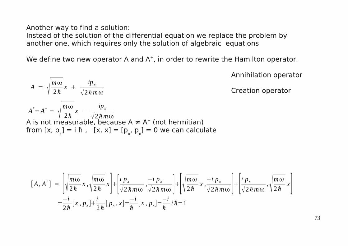
Another way to find a solution:Instead of the solution of the differential equation we replace the problem byanother one, which requires only the solution of algebraic equations
We define two new operator A and A+, in order to rewrite the Hamilton operator.
Annihilation operator
Creation operator
A is not measurable, because A ≠ A+ (not hermitian)from [x, p
x] = i ħ , [x, x] = [p
x, p
x] = 0 we can calculate
A = m2ℏx
ip x
2ℏm
A*=A= m2ℏ
x −ipx
2ℏm
[A , A+] = [m2ℏ
x , m2ℏx ][ i p x
2 ℏm,−i p x
2ℏm ][m2ℏx ,−i p x
2ℏm ][i p x
2ℏm,m2ℏ
x ]=−i2ℏ[ x , px ]
i2ℏ[ px , x ]=
−iℏ[ x , px]=
−iℏ
i ℏ=1

74
x=2ℏm
12 AA+
p x=2ℏm−i2 A−A+
x 2=
ℏ
2m A2AA+
A+AA+2
p x2=−ℏm1
2A2−AA+−A+AA+2
Now we rewrite the Hamilton operator with help of A and A+
H =p x
2
2m
m2
2x 2
A = m2ℏx
ip x
2ℏm
A = m2 ℏx −
ip x
2ℏm
Inserting in Hamilton operator and using the previous result
H = −ℏ
4 A2−AA+
−A+AA+2ℏ
4A2AA+
A+AA+2=ℏ
42 AA+
A+A
=ℏ
22 A+A1=ℏ A+A
12
[A , A+]=A A+
−A+A=1
75
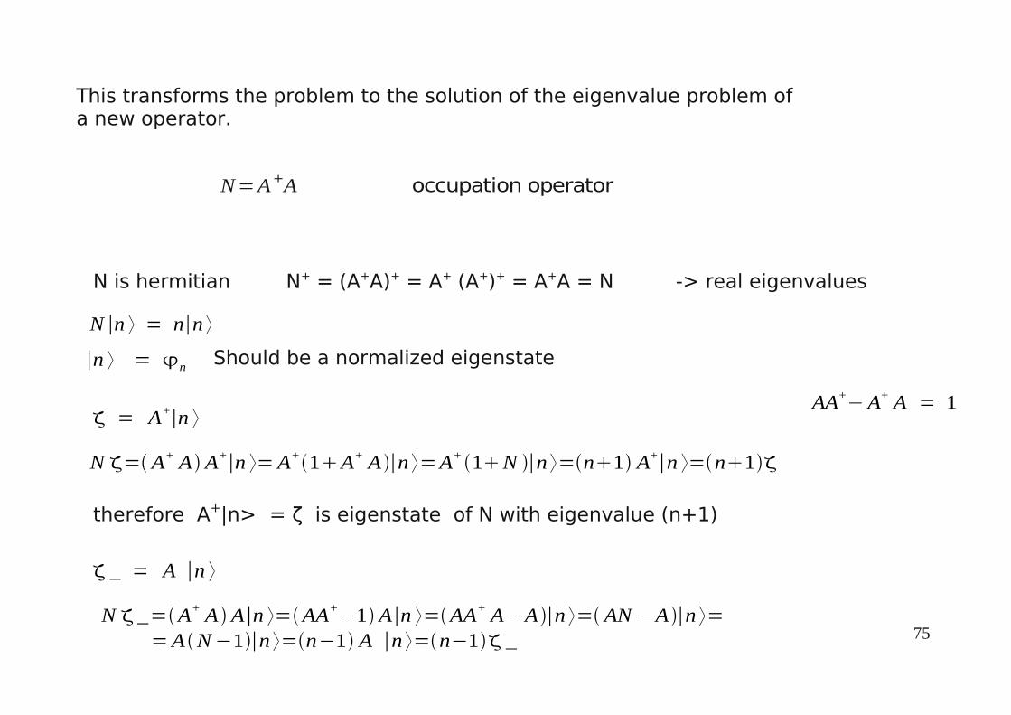
This transforms the problem to the solution of the eigenvalue problem ofa new operator.
N=A+A occupation operator
N is hermitian N+ = (A+A)+ = A+ (A+)+ = A+A = N -> real eigenvalues
N ∣n ⟩ = n∣n ⟩
∣n ⟩ = n Should be a normalized eigenstate
N = A+ A A+∣n ⟩=A+1A+ A ∣n ⟩=A+ 1N ∣n ⟩=n1 A+∣n ⟩=n1
therefore A+|n> = ζ is eigenstate of N with eigenvalue (n+1)
= A+∣n ⟩
_ = A ∣n ⟩
N _=A+ A A∣n ⟩=AA+−1 A∣n ⟩=AA+ A−A ∣n ⟩= AN−A ∣n ⟩=
=A N−1∣n ⟩=n−1 A ∣n ⟩=n−1 _
AA+−A+ A = 1
76
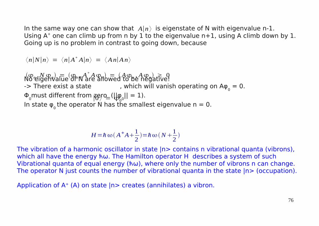
In the same way one can show that is eigenstate of N with eigenvalue n-1.Using A+ one can climb up from n by 1 to the eigenvalue n+1, using A climb down by 1.Going up is no problem in contrast to going down, because
No eigenvalue of N are allowed to be negative!-> There exist a state
, which will vanish operating on Aφ
0 = 0.
Φ0must different from zero (||φ
0|| = 1).
In state φ0 the operator N has the smallest eigenvalue n = 0.
⟨n∣N∣n⟩ = ⟨n∣A+ A∣n⟩ = ⟨An∣An⟩
n , N n = n , A+ An = An , An ≥ 0
A∣n ⟩
∣0 ⟩ = 0
The vibration of a harmonic oscillator in state |n> contains n vibrational quanta (vibrons),which all have the energy ћω. The Hamilton operator H describes a system of such Vibrational quanta of equal energy (ћω), where only the number of vibrons n can change.The operator N just counts the number of vibrational quanta in the state |n> (occupation).
Application of A+ (A) on state |n> creates (annihilates) a vibron.
H=ℏ A+A12=ℏN
12
77
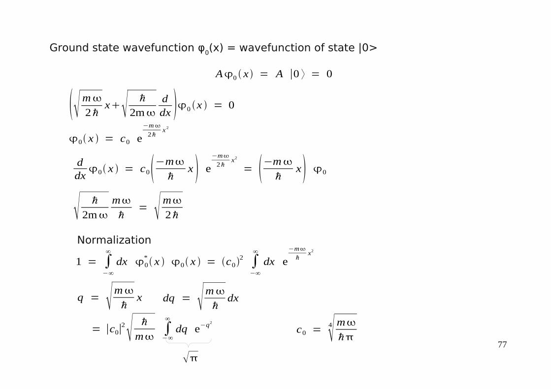
Ground state wavefunction φ0(x) = wavefunction of state |0>
A0 x = A ∣0 ⟩ = 0
m2ℏx ℏ
2mddx 0 x = 0
0 x = c0 e−m
2ℏx 2
ddx0 x = c0−mℏ x e
−m
2ℏx2
= −mℏ x 0
ℏ
2mmℏ
= m2ℏ
Normalization
1 = ∫−∞
∞
dx 0* x 0 x = c0
2 ∫−∞
∞
dx e−m
ℏx2
q = mℏ x dq = mℏ dx
= ∣c0∣2 ℏ
m∫−∞
∞
dq e−q2
c0 =4 mℏ

78
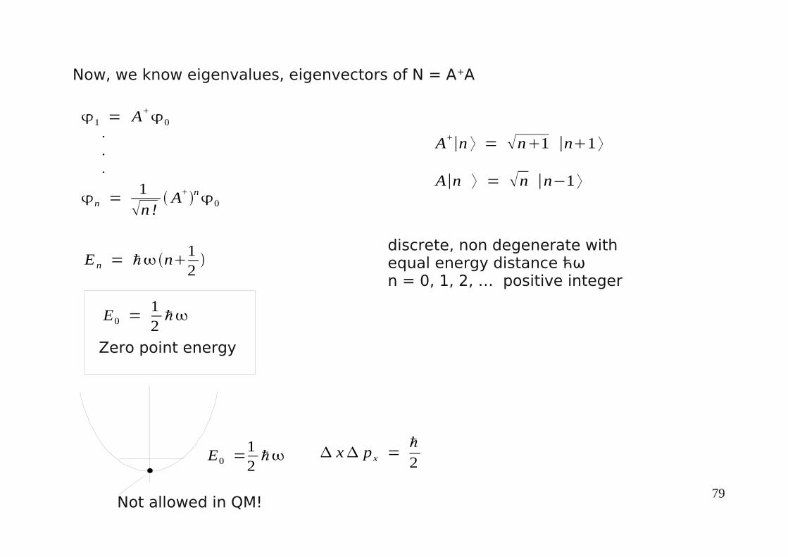
remaining eigenfunctions created by repeatedly operating with A+
1 =1
2 − dd 0 = mℏ
14 1
2 − dd e
−2
2
⋅⋅⋅
n =1
n! 2n − dd
n
0
Hermite Polynomial
H n = ex2
2 x− ddx
n
e−x 2
2 = −1n ex 2 d n
dx ne−x
2
n =1
n ! 2n mℏ 14
e−2
2 H n n = 0, 1, 2, . . .
79
Now, we know eigenvalues, eigenvectors of N = A+A
1 = A+0
⋅⋅⋅
n =1
n ! A+n0
E n = ℏn12
A+∣n ⟩ = n1 ∣n1 ⟩
A∣n ⟩ = n ∣n−1 ⟩
E0 =12ℏ
Zero point energy
Not allowed in QM!
E0 =12ℏ x p x =
ℏ
2
discrete, non degenerate with equal energy distance ћωn = 0, 1, 2, … positive integer

80
The eigenfunction φn has exactly n zeros.
IR-absorption between states of different parity (dipole selection rules)
~ ⟨n∣x∣m ⟩ = ∫n* xmdx
n=0 -> n=1 strong transitionn=0 -> n=2 forbidden (equal parity)
Integral with symmetric limits of an odd function vanishes.

81
Any system which can vibrate (molecules, solids) is approximately a system of coupled harmonic oscillators A transformation to so called „normal coordinates“ changes it into a system of uncoupled 1D harmonic oscillators.
Zero point energies are real and contribute to stability (lowering of binding energies), and therefore also to the total energy and enthalpy.13C is in higher abundance in biological systems compared to inorganic processes.
Confirmation of Planck explanation of black body radiation.
Quantum electrodynamics is formulated usually in terms of creation and annihilationoperators, which means is based on the physics of the harmonic oscillator.
Importance of the harmonic oscillators for physics

82
9.Two level systems
9.1 Ammonia (NH3)
H-atoms form an equal lateral triangle. The energetic favorable location of N is notin the plane of the H-atoms, but above or below at the same distance and same energy.Ammonia has obviously many different states, however we reduce it to a model withonly two states corresponding to the position of the N atom.
Dipole moment d
∣1 ⟩∣2 ⟩
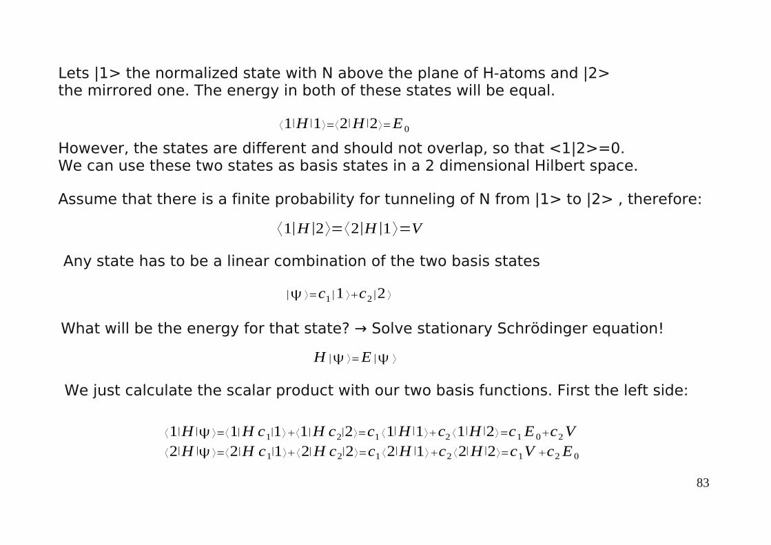
83
Lets |1> the normalized state with N above the plane of H-atoms and |2> the mirrored one. The energy in both of these states will be equal.
⟨1∣H∣1⟩=⟨2∣H∣2⟩=E 0
Assume that there is a finite probability for tunneling of N from |1> to |2> , therefore:
⟨1∣H∣2⟩=⟨2∣H∣1⟩=V
Any state has to be a linear combination of the two basis states
∣ ⟩=c1∣1 ⟩c2∣2 ⟩
What will be the energy for that state? → Solve stationary Schrödinger equation!
H ∣ ⟩=E ∣ ⟩
We just calculate the scalar product with our two basis functions. First the left side:
However, the states are different and should not overlap, so that <1|2>=0.We can use these two states as basis states in a 2 dimensional Hilbert space.
⟨1∣H∣ ⟩=⟨1∣H c1∣1⟩⟨1∣H c2
∣2⟩=c1 ⟨1∣H∣1⟩c2 ⟨1∣H∣2⟩=c1E 0c2V⟨2∣H ∣ ⟩=⟨2∣H c1
∣1⟩⟨2∣H c2∣2⟩=c1 ⟨2∣H ∣1⟩c2 ⟨2∣H∣2⟩=c1V c2E 0

84
The right side of the equations gives us:
⟨1∣E∣ ⟩=⟨1∣E c1∣1⟩⟨1∣E c2
∣2⟩=E c1 ⟨1∣1⟩E c2 ⟨1∣2⟩=E c1
⟨2∣E∣ ⟩=⟨2∣E c1∣1 ⟩⟨2∣E c2
∣2⟩=E c1 ⟨2∣1⟩E c2 ⟨2∣2⟩=E c2
This is nothing else than linear set of equations for c1 and c
2.
c1E 0c2V=E c1
c1Vc2E 0=E c2
Another, mathematical equal from to express this is based on matrices.
E0 VV E 0
c1
c2=E c1
c2
The solution of the eigenvalue problem gives energy E and the c1 and c
2.
Non-trivial solutions are only possible if the determinant vanishes.
E0−E VV E 0−E
c1
c2=0
det E 0−E VV E0−E =E 0−E
2−V 2=0

85
The corresponding eigenfunctions are:
∣+⟩=∣1 ⟩∣2 ⟩
2∣
-⟩=∣1 ⟩−∣2 ⟩
2
If V is positive, than the state with „-“ will be the ground state, because its energy is lower. The energy difference between both states is equal to 2V.
E+=E 0V
E-=E 0−V
As a result we find two solutions for the energy E:
2V=ℏ=h f
Electromagnetic waves with frequency f can stimulate transitions between these states.For NH
3 the frequency will be f=23.87012 GHz (λ=1.2559 cm) and defines the
Frequency standard for microwave technology. NH
3 is absorbing microwaves with that frequency very strongly.
86
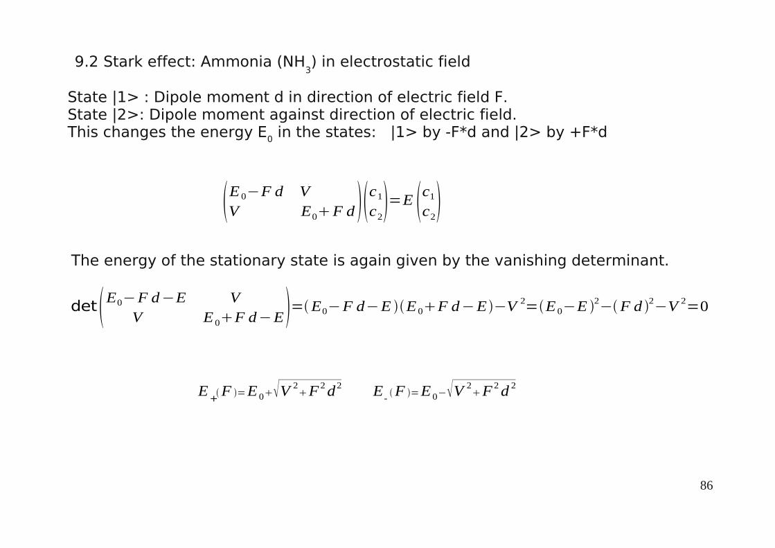
State |1> : Dipole moment d in direction of electric field F.State |2>: Dipole moment against direction of electric field.This changes the energy E0 in the states: |1> by -F*d and |2> by +F*d
9.2 Stark effect: Ammonia (NH3) in electrostatic field
E 0−F d VV E0F d c1
c2=E c1
c2
det E0−F d−E VV E 0F d−E =E0−F d−E E 0F d−E −V 2
=E 0−E 2−F d 2−V 2
=0
The energy of the stationary state is again given by the vanishing determinant.
E+F =E 0V
2F 2d2 E
-F =E 0−V
2F 2d 2

87
For small fields the energy changes quadratic with field, for large fields linear. The change of energy in electric fields is known as linear and quadratic Stark-effect.
Even in case of rather larger electric fields like 10 kV/cm the change corresponds to the quadratic Stark-effect. Compared to electric field strength in atoms these are weak fields.
E+F =E 0V
2F 2d 2 E-F =E 0−V
2F 2d 2
88
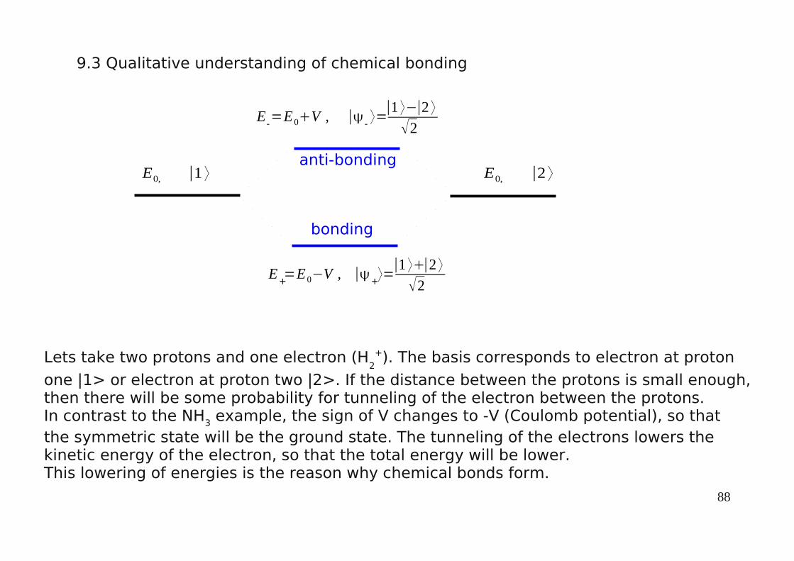
9.3 Qualitative understanding of chemical bonding
E+=E 0−V , ∣
+⟩=∣1 ⟩∣2 ⟩
2
E-=E 0V , ∣
-⟩=∣1 ⟩−∣2 ⟩
2
E0, ∣1 ⟩ E0, ∣2 ⟩
Lets take two protons and one electron (H2
+). The basis corresponds to electron at proton
one |1> or electron at proton two |2>. If the distance between the protons is small enough,then there will be some probability for tunneling of the electron between the protons.In contrast to the NH3 example, the sign of V changes to -V (Coulomb potential), so thatthe symmetric state will be the ground state. The tunneling of the electrons lowers the kinetic energy of the electron, so that the total energy will be lower.This lowering of energies is the reason why chemical bonds form.
bonding
anti-bonding
89
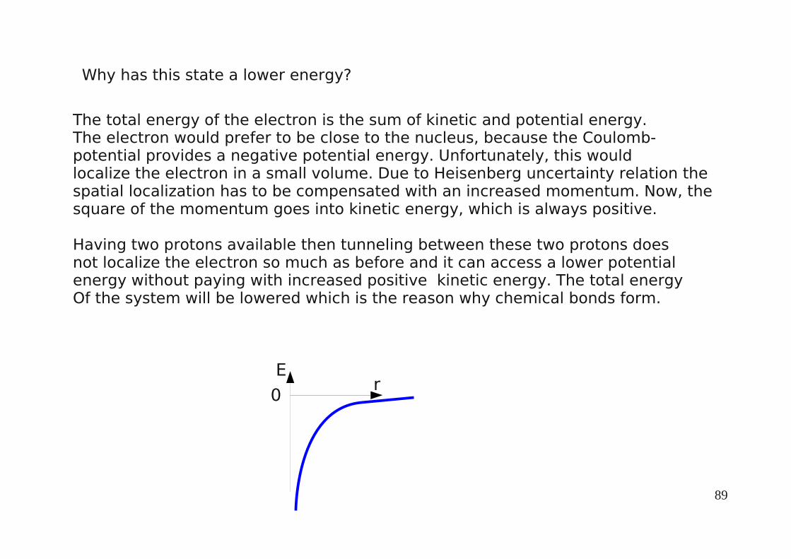
Why has this state a lower energy?
The total energy of the electron is the sum of kinetic and potential energy.The electron would prefer to be close to the nucleus, because the Coulomb-potential provides a negative potential energy. Unfortunately, this wouldlocalize the electron in a small volume. Due to Heisenberg uncertainty relation thespatial localization has to be compensated with an increased momentum. Now, the square of the momentum goes into kinetic energy, which is always positive.
Having two protons available then tunneling between these two protons doesnot localize the electron so much as before and it can access a lower potential energy without paying with increased positive kinetic energy. The total energyOf the system will be lowered which is the reason why chemical bonds form.
rE
0
90
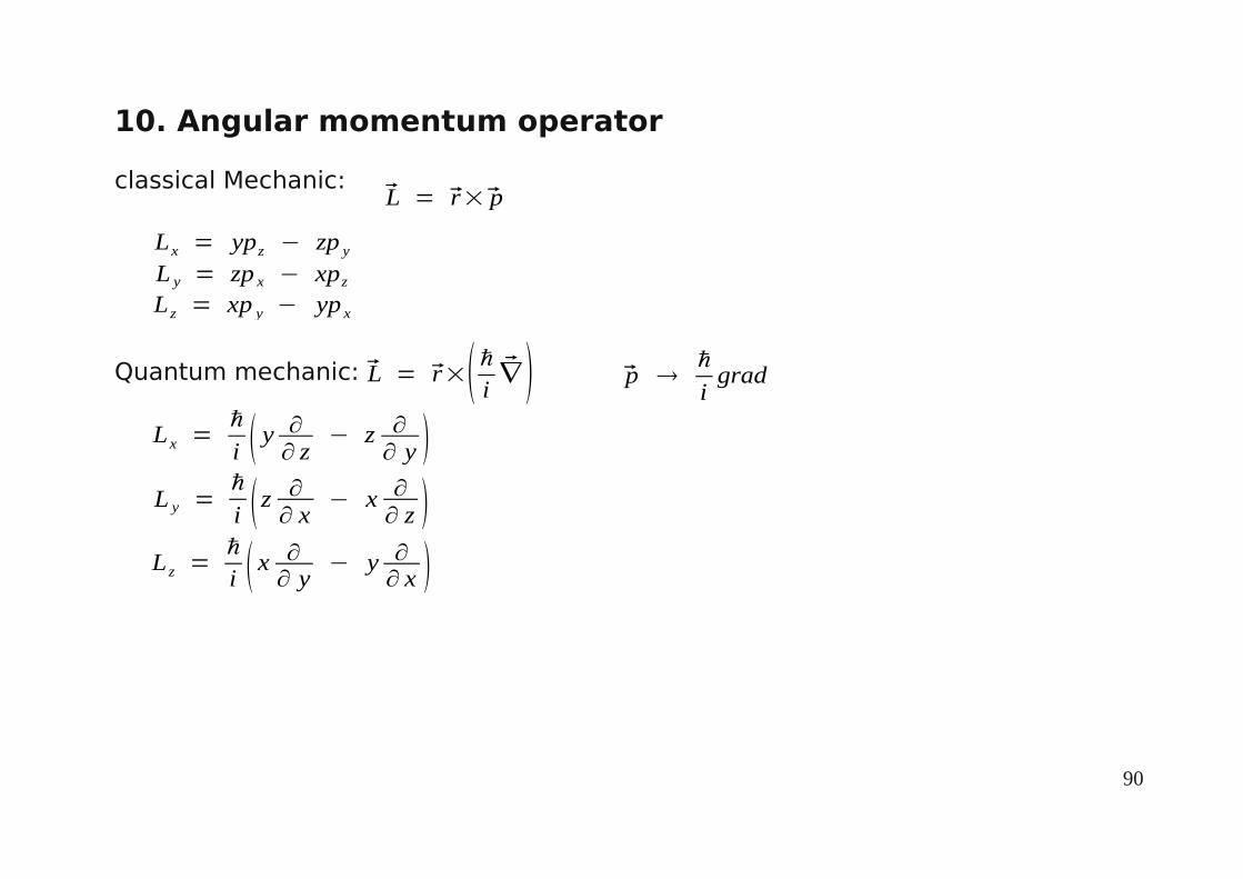
10. Angular momentum operator
classical Mechanic:L = r×p
Lx = ypz − zp y
L y = zp x − xpzLz = xp y − yp x
Quantum mechanic: L = r× ℏi ∇ p ℏ
igrad
Lx =ℏ
i y∂∂ z
− z ∂∂ y
L y =ℏ
i z∂∂ x
− x ∂∂ z
L z =ℏ
i x ∂∂ y − y ∂∂ x

91
Rotations will not change the distance from origin.--> use spherical coordinates (r, φ, )
x = r sin cosy = r sin sinz = r cos
z
x
y
r
φ
We need to replace derivative with respect to x, y, z by there corresponding angularderivatives.
∂∂
=∂ x∂
∂∂ x
∂ y∂
∂∂ y
∂ z∂
∂∂ z
= −r sin sin ∂∂ x
r sin cos∂∂ y
0
= − y∂∂ x
x ∂∂ y
= x ∂∂ y
− y∂∂ x
Lz =ℏ
i∂
∂
92
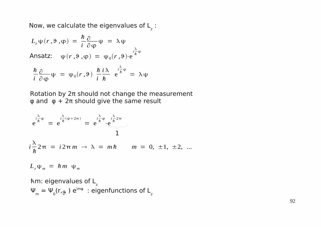
Now, we calculate the eigenvalues of Lz :
Lzr , , =ℏ
i∂∂
=
Ansatz: r , , = 0r ,⋅ei
ℏ
ℏ
i∂∂
= 0r ,ℏ
ii ℏ
ei
ℏ
=
Rotation by 2π should not change the measurement φ and φ + 2π should give the same result
ei
ℏ
= ei
ℏ2
= ei
ℏ
⋅ei
ℏ2
1
i
ℏ2 = i 2m = m ℏ m = 0, ±1, ±2, ...
L zm = ℏm m
ћm: eigenvalues of Lz
Ψm = Ψ
0(r, ) eimφ : eigenfunctions of L
z

93
Can we measure Lx and L
y sharp if we are in an eigenstate Ψ
m ?
Only if the commutatot [Lx, L
y] is zero, one can measure both components sharp.
[ Lx , L y ] = [ y p z − z p y , z p x − x pz ]= y pz − z p y z px − x p z − z px − x p z y pz − z p y
= y p z z px − y z p z p x x z p z p y − x p z z p y
= y pz z − z p z p x x z p z− p z z p y
= y [ p z , z ] p x x [ z , p z ] p y
= − y [ z , p z ] p x x [ z , pz ] p y
i ℏi ℏ
= iℏ x p y − y p x = i ℏ L z
[ Lx , L y ] = iℏ Lz
[ Ly , L z ] = i ℏ Lx
[ Lz , Lx ] = i ℏ L y
The components of the angular momentum operator can not bemeasured at the same time.(Vector L can not have a fixed direction.)
= y p z z px − y p z x p z − z p y z p x z p y x p z − z p x y p z − z px z p y− x pz y p z x pz z p y
94
Eigenfunctions of Lx and L
y are not eigenfunctions of L
z.
How to describe then angular momentum in QM?
L2= Lx
2 L y
2 L z
2
[ L2 , L z ] = [Lx2 , L z ] [L y
2 , L z ] [ Lz2 , Lz ]
0= Lx
2 L z− Lz Lx2 Ly
2 Lz− Lz L y2
= Lx [ Lx , Lz ] [ L x , L z] Lx L y [ L y , Lz ] [ Ly , Lz ] L y
= − i ℏ Lx L y − i ℏ L y Lx i ℏ L y Lx i ℏ L x L y = 0
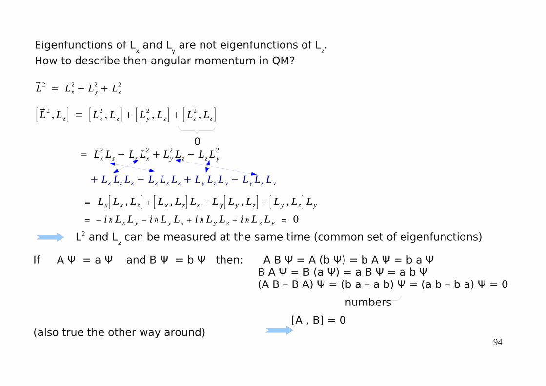
L2 and Lz can be measured at the same time (common set of eigenfunctions)
Lx Lz Lx− Lx Lz Lx L y Lz L y− L y Lz L y
If A Ψ = a Ψ and B Ψ = b Ψ then: A B Ψ = A (b Ψ) = b A Ψ = b a Ψ B A Ψ = B (a Ψ) = a B Ψ = a b Ψ (A B – B A) Ψ = (b a – a b) Ψ = (a b – b a) Ψ = 0
numbers
[A , B] = 0(also true the other way around)

95
Eigenvalues of L2 are needed:
L2 = ≥ 0
,L2 = , Lx
2 , L y
2 , Lz
2
= Lx , Lx L y , L y Lz , Lz
L2= −ℏ
2 [ 1sin
∂∂ sin ∂
∂ 1
sin2
∂2
∂2 ]
L2 contains derivates with respect to both angles -> λ and m are not independent.Ansatz:
r , , = f r Y lm ,
Solving the differential equation (see any text book on QM) gives:
L2Y lm , = ℏ2 l l1 Y lm ,
L z Y lm , = ℏ m Y lm ,
with l = 0 , 1 , 2 , 3 , . . .m = −l ,−l1 , . . . , 0 , . . . , l ∣m∣ ≤ l

96
Y lm , = spherical harmonics)
Y lm , = 2 l14
l−m !lm !
P lm cos ei m
Lz
Legendre-Polynome (adjoint to) l+m
P lm x =
−1m
2l l !1−x2
m2 d lm
d x lm x2−1l
see Messiah, Nolting
s-statel = 0 Y 00 , =
1
4
l = 1 Y 10 , = 34
cos Y 1±1 , = ∓ 38
sin e±i
l = 2 Y 20 =12 5
43cos2−1 Y 2±1 = ∓ 15
8sin cos e±i
Y 2±2 =14 15
2sin2 e±2i
All spherical harmonics for m≠0 are complex!
10.1 Spherical harmonics

97
historical names
l = 0 s-state sharp m = 0l = 1 p-state principal m = -1, 0, 1l = 2 d-state diffuse m = -2, -1, 0, 1, 2l = 3 f-state fundamental m = -3, -2, -1, 0, 1, 2, 3l = 4 g-state
l = 0 ψ(r, ,φ) = ψ(r) no angular momentum, spherical symmetric
Classical picture for L2 und Lz
L moves on sphere
with radius
ℏ l l1
L2ℏ2 l l1 ∣L∣ℏ l l1
Lz
Lz = 0
Lz = ℏ
Lz = −ℏ
l = 1, radius ℏ √2
Lz fixed value, but smaller than the projection if the radius on L
z
Lx, L
y have no fixed values
98
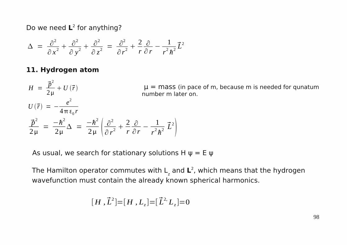
Do we need L2 for anything?
= ∂2
∂ x 2 ∂
2
∂ y2 ∂
2
∂ z2 =∂
2
∂ r2 2r∂∂ r−
1
r2ℏ
2L2
11. Hydrogen atom
H =p2
2U r
U r = −e2
40 r
μ = mass (in pace of m, because m is needed for qunatum number m later on.
p2
2=−ℏ
2
2 =
−ℏ2
2 ∂2
∂ r2 2r∂∂ r−
1r2ℏ
2L2
As usual, we search for stationary solutions H ψ = E ψ
[H , L2]=[H , Lz ]=[L
2, L z ]=0
The Hamilton operator commutes with Lz and L2, which means that the hydrogen
wavefunction must contain the already known spherical harmonics.

99
nlmr , , = f nl r Y lm ,
= [−ℏ2
2 ∂2 f nl r
∂ r 2 2r∂∂ r
f nl r U r f nl r ] Y lmℏ
2
21
r2ℏ
2 ℏ2 l l1 f nl r Y lm
Enlm f nl r Y lm ,
Ansatz:
Differenzial equation for fnl(r) depends on l, but not on the angles itself.
Enlm f nl r = −ℏ2
2 ∂2 f nl r
∂ r2 2r∂∂ r
f nl r U r f nl r ℏ2 l l1
2 r2 f nl r
There is no dependence on m -> Enl
We are interested in bound electrons, fnl(r -> ∞) = 0
fnl(r) = Ansatz as polynomial times exponent
Inserting in differential equation gives constants -> a, b, ... -> done= e−anl r [bnl cnl r dnl r
2 . . . ]
The wavefunction needs to be normalized so that the series has to be finite.This gives a condition for allowed energies (see: Mathematica H-Atom.nb).

100
In particular for U r = −e2
40 r
Enl = E n = −1
n2E 0
no l dependence
E0 =e2
40
12a0
= 13,6 eV = 1 Ry
a0 =ℏ2
40
e2= 0,529177⋅10−10 m Bohr radius
Main quantum number n = 1, 2, 3, . . .Orbital quantum number l = 0, 1, 2, . . . , n-1Magnetic quantum number m = -l, . . . , 0, . . . l
All ions with 1 electron like He+, Li++, . . . can be described in the same way. Only the potential U(r) changes e2 -> Z e2
For a general potential the energy will depend on n and l, in case of the Coulomb potential there is only a dependence on n.
En = −Z 2
n2 E0

101
n = 1 l = 0 s - state m = 0 1 state
n = 2 l = 0 s - state m = 0 4 states l = 1 p - state m = -1, 0, 1
n = 3 l = 0 s - state m = 0
l = 1 p - state m = -1, 0, 1 9 states l = 2 d - state m = -2, -1, 0, 1, 2
Each state can be occupied by 2 electrons! (Reason is spin → see later chapter)
n = 1 K – Shell 2 electrons
n = 2 L – Shell 8 electrons
n = 3 M – Shell 18 electrons

102
11.1 Radial wave part of hydrogen-like atoms
n=1l=0
n=2l=0 l=1
n=3l=0 l=1 l=2
fnl(r) f
nl(r)
fnl(r)
r2fnl(r)2r2f
nl(r)2r2f
nl(r)2
x-axis is for all pictures the radial distance r in units of Bohr radius a0.
The radial functions have n-l-1 zeros and may also become negative.

103
l = 1 Y 10 , = 34
cos Y 1±1 , = ∓ 38
sin e±i
11.2 Construction of real valued angular functions
All spherical harmonics for m≠0 are complex!Building proper linear recombination one can construct completely real valued orbitals.
p x=12Y 1−1−Y 11=
12 3
8sin e−i ei= 3
4sin cos= 3
4xr
p y=i2Y 11Y 1−1=
i2 3
8sin −ei e−i= 3
4sin sin= 3
4yr
p z=Y 10= 38
cos
l = 0 Y 00 , =1
4
s-wavefunction is spherical symmetric (no angular dependence)
p-wavefunction

104
p-orbital l=1
s-orbital l=0
Alonso/Finn: Quantenphysik

105
l = 2 Y 20 =12 5
43cos2−1 Y 2±1 = ∓ 15
8sin cos e±i
Y 2±2 =14 15
2sin2 e±2i
the d-orbitals are constructed the same way:
m=0 d z 2−r 2= 5
163 cos2
−1 = 516
3z2−r2
r 2
m=1 d xz = 154
sin cos cos = 154
xzr 2
m=1 d yz = 154
sin cos sin = 154
yzr2
m=2 d x 2− y2= 15
4sin2
cos2 = 154
x 2− y2
r2
m=2 d xy = 154
sin2 sin 2 = 154
xyr2
d-wavefunction
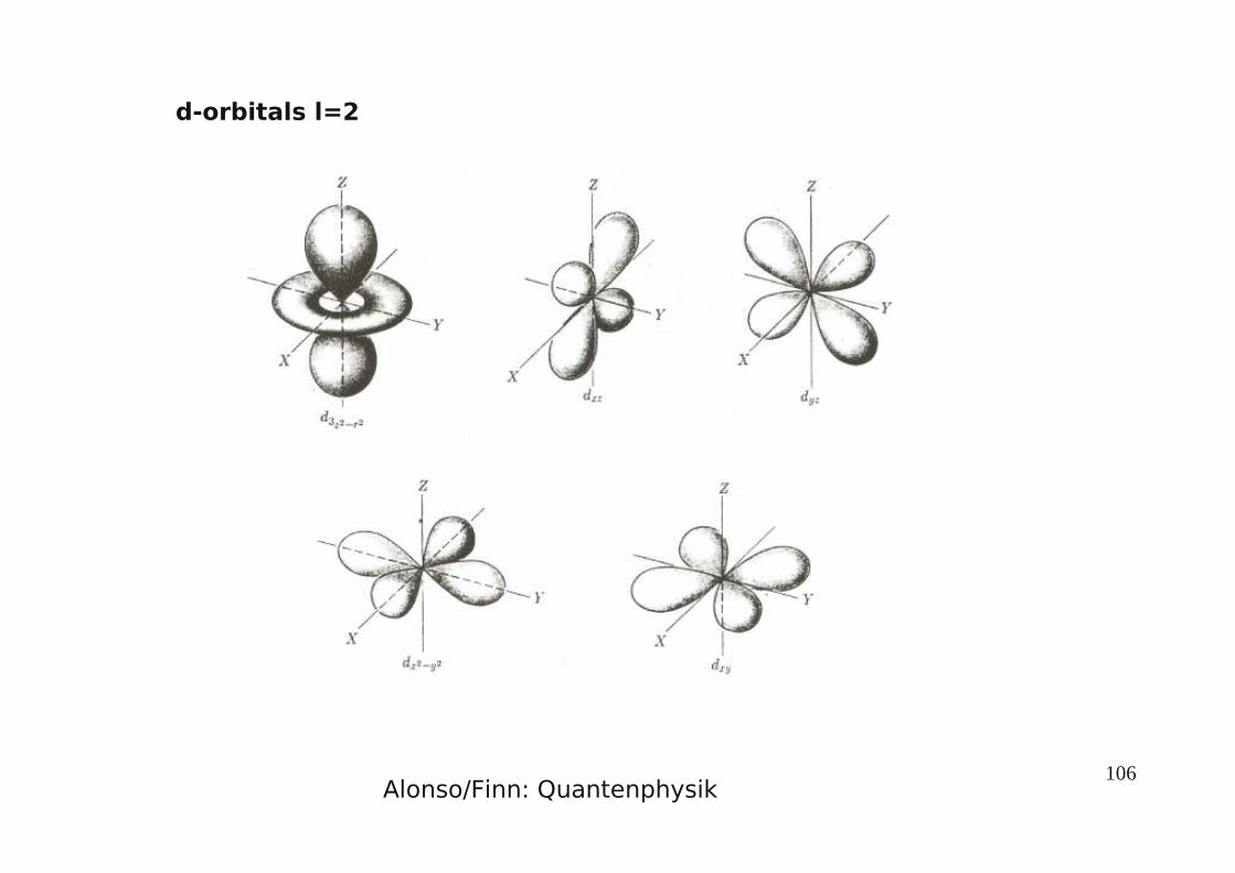
106
d-orbitals l=2
Alonso/Finn: Quantenphysik

107
f-orbitals l=3
m=0
m=±1 m=±2 m=±3
Many more plots and animations of orbitals and densities: http://winter.group.shef.ac.uk/orbitron/
108
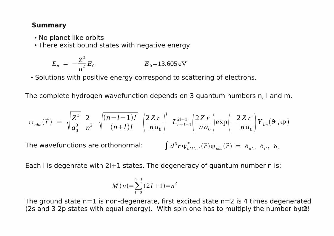
Summary
No planet like orbits There exist bound states with negative energy
En = −Z 2
n2 E0 E 0=13.605 eV
nlmr = Z3
a03
2n2 n−l−1!
nl ! 2Z rna0l
Ln− l−12l1 2Z rna0
exp−2Z rna0
Y lm ,
The complete hydrogen wavefunction depends on 3 quantum numbers n, l and m.
The wavefunctions are orthonormal: ∫d 3 rn ' l ' m '*
r nlm r = n ' n l ' l m' m
Each l is degenrate with 2l+1 states. The degeneracy of quantum number n is:
M n=∑l=0
n−1
2 l1=n2
The ground state n=1 is non-degenerate, first excited state n=2 is 4 times degenerated(2s and 3 2p states with equal energy). With spin one has to multiply the number by 2!
Solutions with positive energy correspond to scattering of electrons.

109
optical transition are governed by the dipole selection rules
l = ±1 m = 0, ±1
0 1 2
n = 1
l
En/E
0
n = 2
n = 3
s p d
Spektral lines
An electron transition is always connected with emission or absorption of a photon.Energy of the photon must exactly equal to the energy difference of participating levels so that the transition can occur.
E=ℏ=2ℏ=2ℏ c /
1= E
2 ℏ c=
Z 2e2
4 a0ℏ c 1
n12 −
1
n22 =RH 1
n12 −
1
n22
For hydrogen gas have been several series observed (n1=1 Lyman, n
1=2 Balmer).
RH=Rydberg constant

110
11.3 further approximation
Instead of the electron mass one should use the reduced mass.
1=
1me
1M
Kern
≈1me
This allows to observe an isotope effect in optical spectra. Deuterium has been found in 1932 measuring the Rydberg constant very accurately R
H/R
D=0.99973.
Fine structure: relativistic corrections (Spin-orbit-coupling, Dirac-equation) Splitting observed in case of p, d and f-states.
Hyperfine structure: Interaction of electron spin with nuclear spin Lamb-shift: Interaction with vacuum (quantum electrodynamics) gives additional splitting (5μeV) of the 2s
1/2 and 2p
1/2 states, which are degenerate in Dirac equation.
Fine structure constant
=40 ℏ
2
me2 ≈ 1/137
Fließbach:Quantenmechanik

111
12. Particles in magnetic fields
v
r
M
Electrodynamics: Charge Q moving in a circular orbit is the same as a current in a loop -> magnetic Dipole
Magnetic moment M= current x area
Qv2 r r2=Qmv
2m r= Q2m r pM=
Q2m
r×p=Q
2mL
E=−M⋅B
The interaction energy of a magnetic dipole M with an external magnetic field B is given by:
112
QM treatment
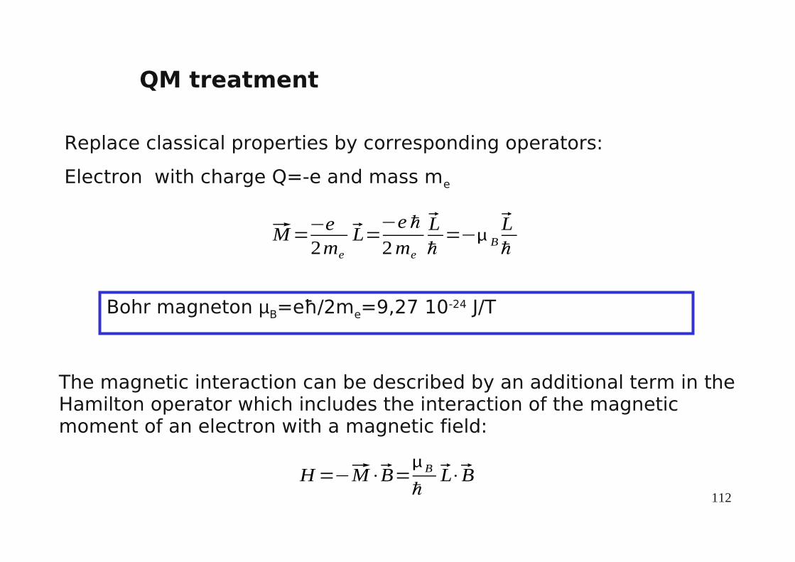
Replace classical properties by corresponding operators:
Electron with charge Q=-e and mass me
Bohr magneton µB=eħ/2me=9,27 10-24 J/T
The magnetic interaction can be described by an additional term in the Hamilton operator which includes the interaction of the magnetic moment of an electron with a magnetic field:
M=−e2me
L=−e ℏ
2me
Lℏ=− B
Lℏ
H=−M⋅B=B
ℏL⋅B
113
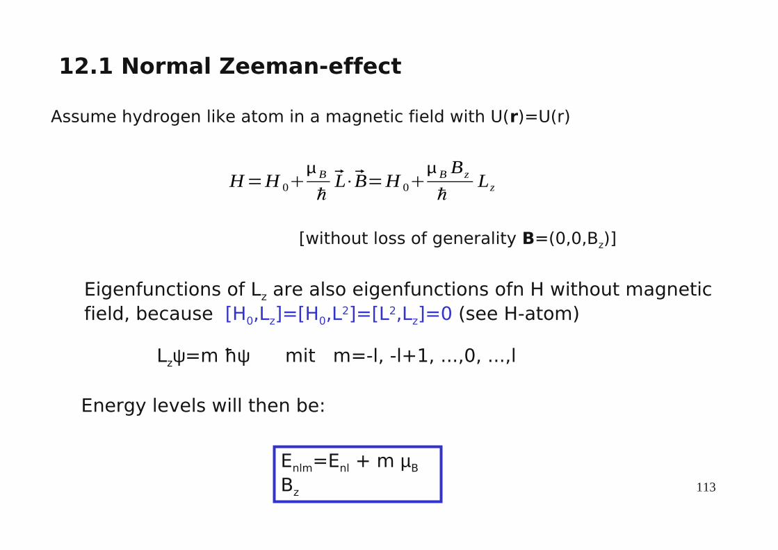
12.1 Normal Zeeman-effect
[without loss of generality B=(0,0,Bz)]
Eigenfunctions of Lz are also eigenfunctions ofn H without magnetic field, because [H0,Lz]=[H0,L2]=[L2,Lz]=0 (see H-atom)
Lzψ=m ħψ mit m=-l, -l+1, ...,0, ...,l
Energy levels will then be:
Enlm=Enl + m µB
Bz
Assume hydrogen like atom in a magnetic field with U(r)=U(r)
H=H 0B
ℏL⋅B=H 0
B Bz
ℏLz

114
normal Zeeman-effect
(2l+1) degnerate stateswuth m = -l,…+l
(2l+1) states with different energy
m = 0
m = -1
m = +1
E3d
B=0 B≠ 0
m = -2
m = +2µB Bz
Enlm=Enl + m µB Bz
Splitting in 2l+1 levels by an external magnetic field.
This is the reason for calling m magnetic quantum number.
e.g. atom with d-electrons (d -> l=2)

115
Numebr of spectral lines
m = 0
m = -1
m = +1
E3d
B=0B≠ 0
m = -2
m = +2
m = 0
m = -1
m = +1
E2p
l=1
l=2
ΔE
ΔEΔE+μBB ΔE-μ
BB
Selection rules: Δl=1, Δm=-1, 0, 115 possible combinations, 9 transitons allowed by dipole selection rules3 mesurable spectral lines, because the levels have equal energy distances.

116
13. Spin
Experimental facts:
1. Normal Zeeman-effect is the exception: Most often one observes the anormal Zeeman-effect (additional splittings)
2. Fine structure of alkali elements : Yellow D-line of Na is a doublet instead of a single line.
3. Stern-Gerlach experiment
Pictures and information on Stern-Gerlach experiment are fromPhysics Today December 2003: Friedrich and Herschbach, "Stern and Gerlach: How a Bad Cigar Helped Reorient Atomic Physics"
http://www.physicstoday.org/vol-56/iss-12/p53.html

117
13.1 Stern-Gerlach experiment (1921/1922)
An inhomogeneous magnetic field produces a force acting on a magnetic moment, because F = - grad E
Therefore, particles with different magnetic quantum number m should experience different forces, so that the beam should split.
F=∇ M⋅B=∇ − B
ℏL z Bz =−m B
d B z
dz

118
Stern-Gerlach-experiment
Splitting in 2 beams in case of Ag, but no splitting in case of Ag+.The calculated magnetic moment for Ag equals 1 µB.
Otto Stern17.2.1888 Sohrau
†17.8.1969 Berkeley
Physik-Nobelpreis 1943
W. Gerlach 1.8.1889 Biebrich am Rhein
†10.8.1979 München
Post card 8 February 1922 to Niels Bohr
119
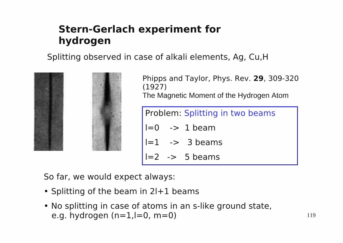
Phipps and Taylor, Phys. Rev. 29, 309-320 (1927) The Magnetic Moment of the Hydrogen Atom
Problem: Splitting in two beams
l=0 -> 1 beam
l=1 -> 3 beams
l=2 -> 5 beams
Splitting observed in case of alkali elements, Ag, Cu,H
Stern-Gerlach experiment for hydrogen
So far, we would expect always:
• Splitting of the beam in 2l+1 beams
• No splitting in case of atoms in an s-like ground state, e.g. hydrogen (n=1,l=0, m=0)

120
13.2 Explanation of the Stern-Gerlach experiment
1925 by Uhlenbeck and Goudsmit after an idea of Pauli:
Elektrons have a permanent magnetic moment = spin
Goudsmit Uhlenbeck Pauli
In complete analogy to angular momentum we define spin operators with spin quantum numbers s and ms.
Also identical commutator relations:
Lz Y lm ,=m ℏY lm ,L2Y lm ,=l l1ℏ2Y lm ,
s=12, −s≤ms≤s ms±
12
S=S x , S y , S z
S z s ,ms=msℏ s ,m s
=±12ℏ s ,m s
S 2 s ,ms
=s s1ℏ2 s ,ms
=34ℏ
2 s ,ms
[S x , S y ]=i ℏS z [ Lx , L y]=i ℏ Lz

121
13.2 Pauli matrices
Possible representation of S using Pauli matrices σ = (σx,σy ,σz):
These matrices fulfill all commutator relations (home work :-).
The wavefunction becomes a vector with two components (spinor).
z=1 00 −1 x=0 1
1 0 y=0 −ii 0
S=ℏ
2
=1r ,t 102r ,t 01 = 1r , t +2r ,t -

122
Quantitative analysis of experiments
The total angular momentum is given by vector addition of orbital momentum and spin J=L+S. The total magnetic moment is however not proportional to J, but is given by:
The Landé-factor g is for an electron equal to 2 within relativistic Dirac theory. Quantum electrodynamics gives g=2.00231930437... ≈ 2 (1+α/2π + ...).
M=−e
2me
L−eme
S = −e
2me
Lg S
Using the matrices the Hamilton operator becomes itself matrix form.
H=H 0 00 H 0
eB2m Lz 0
0 Lz e
mℏ
2B 1 0
0 −1
123
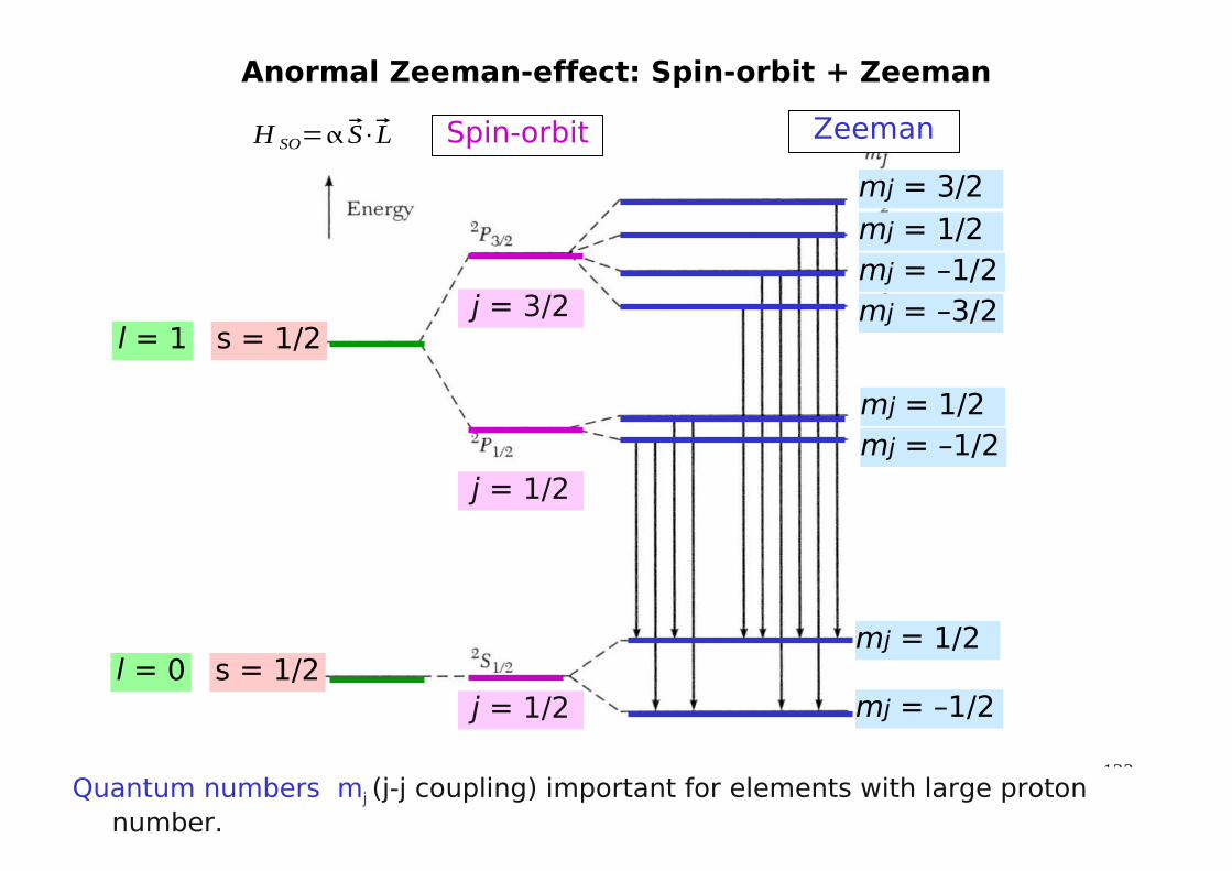
Anormal Zeeman-effect: Spin-orbit + Zeeman
Quantum numbers mj (j-j coupling) important for elements with large proton number.
j = 3/2
j = 1/2
j = 1/2
mj = 1/2
mj = 3/2
mj = –1/2
l = 1mj = –3/2
mj = 1/2mj = –1/2
mj = 1/2
mj = –1/2
Spin-orbit Zeeman
s = 1/2
l = 0 s = 1/2
H SO=S⋅L

124
13.4 Complete set of quantum numbers for H-atom
To describe a state of the H-atom uniquely, we need the main quantum number n, orbital quantum number l, magnetic quantum number m and spin quantum number ms.
The spin functions χ are independent on position and time. The spin represents a fundamental property of the electron, which has no classical counter part.
Hamilton operator for H-atom im magnetic field:
H = H 0B
ℏB⋅Lg S
n l mm sr = Rnl r Y lm ,ms
1/2 = 10 −1/2 = 01

125
13.5 Fermions and Bosons
Not only electrons have a spin but also neutrons, protons, positrons etc.
Particles with half-integer spin are called Fermions, with integer spin bosons.
Fermions: e, n, p, e+ (s=1/2), Ω- (s=3/2)
All matter is build from fermions!
Bosons: photon (s=1), graviton (s=2)
All interactions are exchanged by bosons!
Spin can be a result of vector addition of spin of several particles.
(e.g. nuclear spins s=3/2 state of 57Fe)

126
13.5 Fermions and Bosons
Not only electrons have a spin but also neutrons, protons, positrons etc.
Particles with half-integer spin are called Fermions, with integer spin bosons.
Fermions: e, n, p, e+ (s=1/2), Ω- (s=3/2)
All matter is build from fermions!
Bosons: photon (s=1), graviton (s=2)
All interactions are exchanged by bosons!
Spin can be a result of vector addition of spin of several particles.
(e.g. nuclear spins s=3/2 state of 57Fe)

127
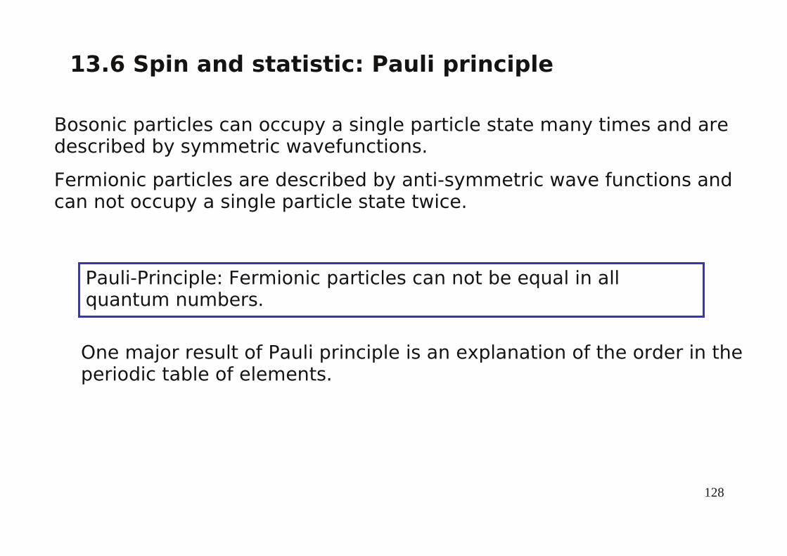
13.6 Spin and statistic: Pauli principle
Bosonic particles can occupy a single particle staremany times and are described by symmetric wavefunctions.
Fermionic particles are described by anti-symmetric wave functions and can not occupy a single particle state twice.
Pauli-Principle: Fermionic particles can not be equal in all quantum numbers.
One major result of Pauli principle is an explanation of the order in the periodic table of elements.
128
13.6 Spin and statistic: Pauli principle
Bosonic particles can occupy a single particle state many times and are described by symmetric wavefunctions.
Fermionic particles are described by anti-symmetric wave functions and can not occupy a single particle state twice.
Pauli-Principle: Fermionic particles can not be equal in all quantum numbers.
One major result of Pauli principle is an explanation of the order in the periodic table of elements.

129
14 Periodic table14.1 Atoms with many electrons
0 1 2
n = 1
l
En/E
0
n = 2
n = 3
ground stateH (1s)1
He (1s)2
Li (1s)2 (2s)1
oder (1s)2 (2p)1
Be (1s)2 (2s)2
(1s)1 (2s)1 (2p)1
(1s)2 (2p)2
Something has to be different to the H-atom!
Improved approximation:Each electron interacts with the positive nucleus with Z protons and interacts with the other Z-1 electrons of the atom.
Potential U(r) is not the Coulomb potential anymore!
En=−1
n2Ry

130
However, then there are no analytic solutions possible. One has to use approximationsand numerical methods. Result: E
nl instead E
n , E
nl increases mostly with l.
0 1 2
n = 1
l
En/E
0
n = 2
n = 3
Degeneracy for l lifted.Degeneracy with respect to m remains.
Li (1s)2 (2s)1 unique configuration
Until Ar (Z = 18) the periodic table behaves normal, then however one finds E
3d ≈ E
4s
3d – states can be above or below with respect to the 4s – statesSimilar for 4d above/below 5s, 5d above/below 6s
anomal occupation of side group elements 4f (lanthanide) and 5f (actinide) show anormal behavior.
Many-body effects and relativistic correction will deliver the correct ordering.

131
Orginal work of Mendelejew 1869 on the periodic table.
Clemens Winkler, Prof.
In chemistry at Bergakademie Freiberg finds in 1886 the element Germanium in the mineral Argyrodit mined at Grube Himmelsfürst close to Freiberg.
132
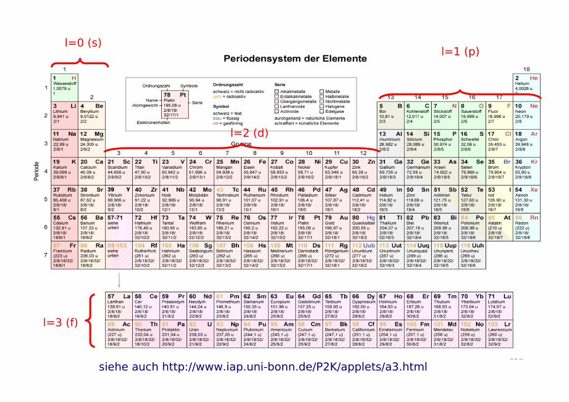
l=0 (s)l=1 (p)
l=2 (d)
l=3 (f)
siehe auch http://www.iap.uni-bonn.de/P2K/applets/a3.html
133
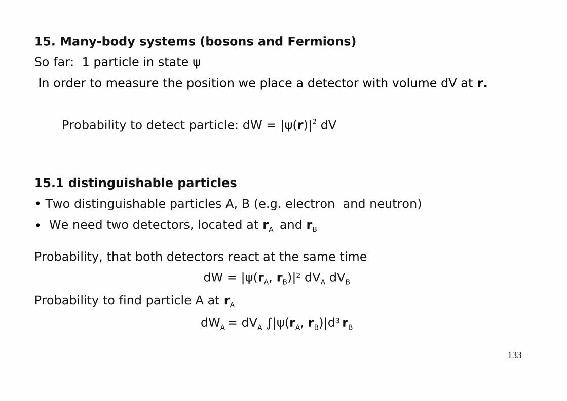
15. Many-body systems (bosons and Fermions)
So far: 1 particle in state ψ
In order to measure the position we place a detector with volume dV at r.
Probability to detect particle: dW = |ψ(r)|2 dV
15.1 distinguishable particles
• Two distinguishable particles A, B (e.g. electron and neutron)
• We need two detectors, located at rA and rB
Probability, that both detectors react at the same time
dW = |ψ(rA, rB)|2 dVA dVB
Probability to find particle A at rA
dWA = dVA ∫|ψ(rA, rB)|d3 rB

134
Sum over all possible positions rB for particle B, because B can anywhere in space.
Similar: Probability, to detect particle B, without being interested in particle A.
dWB = dVB ∫|ψ(rA, rB)| d3 rA
Spin will not really change the discussion, but will just add an additional degree of freedom:
ψ(rA, rB) -> ψ(rA,sA, rB,sB)
Up to now there was not really anything new. This is fully in accord with ourclassical expectations.
2T : , , ,
dW A = dV A ∑sA
∑sB
∫∣ r A , sA , rB , sB∣ d 3rB

135
15.2 Two identical particles (electrons)
Instead using A, B we will label the electrons with 1 and 2
• at r1 we have positioned detector 1 with dV1
• at r2 we have positioned detector 2 with dV2
If both detectors give a signal at the same time, then we know that there has been an electron at r1 and at r2.
Which electron created the signal at detector 1? Was it electron 1 or electron 2?
This question can not be answered, because electrons are really indistinguishable particles, they are absolutely identical.
The main difference in quantum mechanics is, that the two-particle wavefunctions ψ(r1, r2) and ψ(r2, r1) may be different.
ψ(r1, r2): first electron at r1 and second electron at r2
ψ(r2, r1): other way around

136
Even if the squares are equal, we have two possible solutions for the wavefunctions which differ in sign.
A) Symmetric wavefunctions
ψ(r1, r
2) = ψ(r
2, r
1)
(Symmetric functions remain symmetric by additions and multiplication with scalars.)
This solution corresponds in nature to particles with integer spin (0, 1, 2, ...).
(e. g. pion, He, photonen, . . . = Boson)
In particular the many-body wavefunction can be a product of single-particle states.
Bosons can occupy single-particle states several times.
(Bose-Einstein-condensate: Nobel prize 2001)
r1 r2 = r1 r2
∣ r1 , r 2∣2= ∣ r 2 , r 1∣
2
Based on the experiment it has to hold that:

137
B) anti-symmetric wavefunction
Particles with half-integer spin (s = ½, 3/2, . . . )e.g. electron, proton, myon, neutrino, . . . = Fermion
Spin state is important here!
ψ(r1, s
1, r
2, s
2 ) = -ψ(r
2, s
2, r
1, s
1)
The anti-symmetric behavior of the many-body wavefunction under particle exchange is nothing else than the well known Pauli principle.
It is not possible to have a fermionic state given by a product of one-particle states
r1 s1 , r2 s2 = r1 , s1 r2 , s2
r2 s2 , r1 s1 = r2 , s2 r1 , s1
= r1 , s1 r2 , s2
1 = -1Φ = 0 !
Fermions can not occupy the same single-particle state several times. |ψ|2=0
Periodic table of elements

138
Hydrogen atom n, l, m, s
He: 1s n, l, m are equal but s is different
allowed
forbidden
allowed
+
+
+
+ +a
allowed
because 1 r −a2 und 2r
a2 depend on different arguments
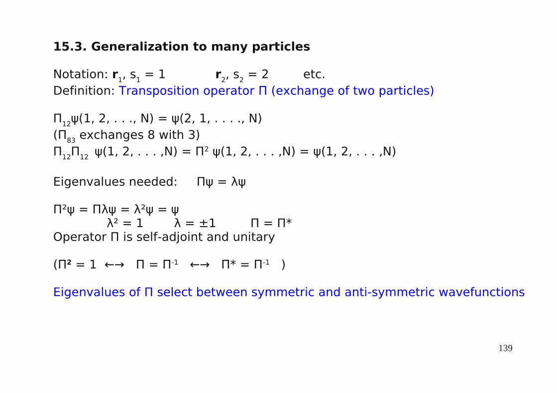
139
15.3. Generalization to many particles
Notation: r1, s1 = 1 r2, s2 = 2 etc.Definition: Transposition operator Π (exchange of two particles)
Π12ψ(1, 2, . . ., N) = ψ(2, 1, . . . ., N)(Π83 exchanges 8 with 3)Π12Π12 ψ(1, 2, . . . ,N) = Π2 ψ(1, 2, . . . ,N) = ψ(1, 2, . . . ,N)
Eigenvalues needed: Πψ = λψ
Π²ψ = Πλψ = λ²ψ = ψ λ² = 1 λ = ±1 Π = Π*Operator Π is self-adjoint and unitary
(Π2 = 1 ←→ Π = Π-1 ←→ Π* = Π-1 )
Eigenvalues of Π select between symmetric and anti-symmetric wavefunctions

140
Boson: Every particle can be exchanged with any other particle
B1,2 ,3=[ 1,2,3 1,3 ,2 3,2,12,1,3 3,1,2 2,3,1 ]
The bosonic wavefunction ψB has to be normalized.
In general one can build a bosonic many-body wavefunction by permutating all coordinates.
B=∑

141
Fermion
F = [ 1,2 ,3 − 1,3 ,2− 2,1,3 2,3 ,1 3,1 ,2 − 3,2,1 ]
χ(Π) = character of permutation
+1 for even number of exchanges
-1 for odd number of exchanges=
F = ∑
This will give determinants, if Ψ is expressedas product of single-particle functions.

142
H = ∑i
H i = 11⋅22
H i i = E i i
N = 2F =
1
211 22 − 2 1 12
=1
2∣1 1 1221 22∣
Just from normalization if the single-particlewavefunctions are normalized.
1
2
N = 3
F =1
3 !∣11 12 132 1 22 2331 3 2 33
∣F =
1
N !∣11 1N
⋮N 1 N N
∣N
are called Slater-Determinants

143
Helium atom: 2 electrons
H =p1
2
2p2
2
2 V r1 V r 2 V ∣r1−r 2∣
Coulomb-interaction
Assume the solution, Hψ = Eψ is known
= r 1, s1 , r 2 , s2 = 1,2
H = E We want to proof that it holds:
H 1,2 1,2 = E1,2
1 <-> 2 exchange
H 2,12,1 = E2,1 = E [1,2 ]Further, it is true that H 1,2 = H 2,1
H 2,1 2,1 =H 1,22,1 =H 1,2 1,2
HΠψ=EΠψ=ΠEψ(Π−1HΠ)ψ=Eψ=H ψΠ−1HΠ=H HΠ=ΠH [H ,Π ]=0
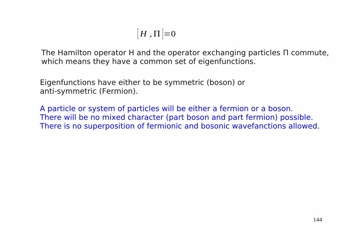
144
The Hamilton operator H and the operator exchanging particles Π commute, which means they have a common set of eigenfunctions.
[H , ]=0
Eigenfunctions have either to be symmetric (boson) or anti-symmetric (Fermion).
A particle or system of particles will be either a fermion or a boson.There will be no mixed character (part boson and part fermion) possible.There is no superposition of fermionic and bosonic wavefanctions allowed.

145
16. Approximate methods
He-atom has 2 electrons
H=∑i=1
2
pi2
2−
Ze2
4 0
1r i
H i
e2
4 0
⋅1
∣r1−r2∣Coulomb-between electrons
H=∑i
H i12∑i≠ j
V ij
What are the stationary solutions ? H =E
.
The solution for independent particles (no e-e interaction) is known form the solution of the Hydrogen atom.However, the e-e interaction depends on the position of both electrons. This does not allow for separation of the problem. For a small number of electrons one can use numerical methods to solve the problem exactly. The numerical complexity and demand increases exponentially with number of electrons, so that one needs approximate methods to find a solution for realistic problem sizes.

146
Why do we need approximate methods?
Example oxygen: O has 8 electronsThe many-body wavefunction depends on position of all 8 electrons.
r1 , r 2 , r3 , r4 , r5 , r 6 , r7 , r 8 24 coordinates
To save the wavefunction we need ψ as function of 24 coordinates. 10 values per coordinate 1024 values 8 bytes per entry 1025 bytes 8.5*109 bytes per DVD 1015 DVD's 10g per DVD 1010 tons
If there would be a method which would need only the charge density instead of the full many-body function the problem would be orders of magnitude easier to handle.
Walter Kohn John Pople
ρ(r) -> 103*8 byte ~ 8 kbyteNobel prize Chemistry 1998: Walter Kohn and John Pople.
Density Functional Theory = DFTThe total energy is a functional of the electron density.