compliant - de lasa · compliant w alking of the scout ii quadr uped martin de lasa ... alebi, a...
TRANSCRIPT

DYNAMIC COMPLIANT WALKING OF
THE SCOUT II QUADRUPED
Martin de Lasa
Department of Electrical and Computer Engineering
McGill University, Montr�eal, Canada
A Thesis submitted to the Faculty of Graduate Studies and Research in partial
ful�llment of the requirements of the degree of
Master of Engineering
c Martin de Lasa, July 2000

Abstract
This research presents the development of a novel dynamic walking controller
for a simple quadrupedal robot, Scout II. Since Scout II does not have knees,
a modi�ed version of the bound, which we call a walking bound was studied.
To gain understanding of system behaviour, an iterative approach of simu-
lation, analysis, and experimentation was pursued. First a simulation study
used in the development of rocking and walking controllers was undertaken.
Attempts to experimentally implement the mentioned controllers revealed un-
modelled dynamics having signi�cant e�ects on system behaviour. Therefore,
another walking algorithm based on commanding constant hip velocity was
experimentally developed. This algorithm proved successful, yielding stable
walking for narrow ranges of operating conditions despite a simple open loop
strategy using minimal feedback. Typical mechanical and electrical power, as
well as speci�c resistance for Scout II compliant walking are quanti�ed.
i
R�esum�e
Cette th�ese pr�esente le d�evelopement d'un nouveau controleur de marche dy-
namique pour Scout II, un robot quadrup�ede simple. Puisque Scout II n'a pas
de genoux, nous avons d�evelop�e une marche dans laquelle les paires de jambes
ant�erieures et post�erieures fonctionnent ensemble. Pour mieux comprendre
le comportement de ce syst�eme, nous avons utilis�e une m�ethode it�erative de
simulation, d'analyse et d'exp�erimentation. D'abord nous avons simul�e deux
algorithmes de marche qui nous ont aid�es �a mieux comprendre le comporte-
ment du syst�eme. N�eanmoins, �a cause de facteurs dynamiques inattendus, ces
algorithmes n'ont pas fonctionn�es sur notre plateforme exp�erimentale. Nous
avons donc d�evelop�e un autre controleur, cette fois experimentalement, dont
le but �etait de commander une vitesse constante aux hanches du robot. Cet
algorithme a bien fonctionn�e pour une s�erie de conditions limit�ees, meme si
c'�etait un controleur simple �a boucle ouverte. La puissance m�ecanique et
�electrique, et la r�esistance sp�eci�que de Scout II ont aussi �et�e mesur�ees.
ii

Acknowledgements
Throughout the course of my research I have received immeasurable guidance,
support, and friendship from numerous individuals. In particular I would like
to thank :
� Professor Martin Buehler, my supervisor, for his help and guidance
through the course of my thesis. Martin's approach to research and
willingness to tackle the daily obstacles I encountered, were sources of
support and encouragement for me. His e�orts to make the ARL a fun
and motivating place to work made my graduate experience a memorable
one.
� The Natural Sciences and Engineering Research Council of Canada (NSERC)
for their support of my work through a graduate scholarship.
� Shervin Talebi, a good friend and irreplaceable colleague. Shervin was
always up for a good debate and willing to have me bounce ideas o�
him. His help and generosity in all aspect of my research can not be
overstated.
� Geo� Hawker for maintaining the lab's PC in running order, getting
QNX running on Scout, and for helping to make the four o'clock Quake
deathmatch an ARL ritual.
� Dave McMordie for reenergizing the ARL and showing all of us that there
is no shame in frying electronics. Dave's positive attitude, unending
imagination, and energy are an inspiration to me.
� Robert Battaglia for building an excellent robotic platform that we have
all bene�ted from. Scout has managed to take considerable abuse and
iii

iv
grief from various \trainers" and still manages to amazes us with its
gracefulness and animal like qualities.
� Ken Yamazaki, for welcoming me into the ARL family and letting me
shadow him when I was still wet behind the ears. Ken's quiet disposition
and kindness made me feel at home from the time I arrived in the lab.
� Mojtaba Ahmadi for his kindness to me when I �rst joined the ARL.
Mojtaba did not hesitate to help make my move to Montreal a pleasant
one.
� Don Campbell for his excellent work on Scout's electronics. Starting
with the now irreplacable IR module and onto more recent projects, I
have had a great time working with him.
� Sami Obaid for his work on Scout's sensors and electronics. His work
was an invaluable resource in the electronics design stage of my thesis.
Sami always lit up the lab with his energy and warmth.
� Didier Papadopoulos for his breakthrough work with Scout. Didier
helped give all of us hope that one day our locomotion algorithms would
also work.
� Ned Moore for making sure we always had some music to lighten up the
lab.
� Liana Mitrea for all her kind gestures and for always bringing something
sweet to the lab for us to enjoy.
� CIM's current and past secretarial sta� : Ornella Cavaliere, Cynthia
Davidson, and Kathleen Vandernoot for helping with rush courier deliv-
eries, emergency faxes and kind smiles.
� Marlene Gray, CIM's manager, for her support and friendship. Marlene
always made sure to drop in and check that things were advancing. Her
small attentions did not go unnoticed.

v
� Jan Binder, CIM's network administrator, for keeping the computer
network running smoothly and saving me from a few unexpected deletes
of the lab web page.
� To my family and new parents in law who supported me through this
often diÆcult experience, thank you for your love and support.
� Lastly I would like to especially thank my wife Magdalena Krol. Her
support, encouragement, and con�dence in me through the more testing
times of my Master's, helped make this thesis a reality. Her contributions
are beyond words.

Contents
1 Introduction 1
1.1 Overview . . . . . . . . . . . . . . . . . . . . . . . . . . . . . . 1
1.2 Motivation . . . . . . . . . . . . . . . . . . . . . . . . . . . . . 2
1.3 Approach . . . . . . . . . . . . . . . . . . . . . . . . . . . . . 3
1.4 Contributions . . . . . . . . . . . . . . . . . . . . . . . . . . . 4
1.5 Thesis Organisation . . . . . . . . . . . . . . . . . . . . . . . . 4
2 Background 6
2.1 Overview . . . . . . . . . . . . . . . . . . . . . . . . . . . . . . 6
2.2 Animal Locomotion Gaits . . . . . . . . . . . . . . . . . . . . 6
2.2.1 The Walk . . . . . . . . . . . . . . . . . . . . . . . . . 7
2.2.2 The Amble . . . . . . . . . . . . . . . . . . . . . . . . 7
2.2.3 The Trot . . . . . . . . . . . . . . . . . . . . . . . . . . 8
2.2.4 The Rack . . . . . . . . . . . . . . . . . . . . . . . . . 9
2.2.5 The Canter . . . . . . . . . . . . . . . . . . . . . . . . 9
2.2.6 The Gallop . . . . . . . . . . . . . . . . . . . . . . . . 9
2.2.7 The Ricochet and the Pronk . . . . . . . . . . . . . . . 10
2.2.8 The Bound . . . . . . . . . . . . . . . . . . . . . . . . 12
2.3 Control of Legged Robots . . . . . . . . . . . . . . . . . . . . 12
2.4 Control of Dynamically Stable Legged Robots . . . . . . . . . 15
2.4.1 Control of Running Robots . . . . . . . . . . . . . . . 15
2.4.2 Control of Walking Robots with Articulated Legs . . . 18
2.4.3 Passive Dynamics in Legged Robot Control . . . . . . 25
2.5 Summary . . . . . . . . . . . . . . . . . . . . . . . . . . . . . 29
vi

CONTENTS vii
3 Scout II 30
3.1 Overview . . . . . . . . . . . . . . . . . . . . . . . . . . . . . . 30
3.2 Platform Speci�cations . . . . . . . . . . . . . . . . . . . . . . 30
3.2.1 Mechanical Subsystem . . . . . . . . . . . . . . . . . . 31
3.2.2 Electrical Subsystem . . . . . . . . . . . . . . . . . . . 32
3.2.3 Software Subsystem . . . . . . . . . . . . . . . . . . . . 36
3.3 Summary . . . . . . . . . . . . . . . . . . . . . . . . . . . . . 43
4 Modeling 44
4.1 Overview . . . . . . . . . . . . . . . . . . . . . . . . . . . . . . 44
4.2 Simulation Package . . . . . . . . . . . . . . . . . . . . . . . . 45
4.3 Rocking . . . . . . . . . . . . . . . . . . . . . . . . . . . . . . 46
4.3.1 Rocking Model . . . . . . . . . . . . . . . . . . . . . . 47
4.3.2 Open Loop Rocking Controller . . . . . . . . . . . . . 50
4.3.3 Simulation Results . . . . . . . . . . . . . . . . . . . . 51
4.3.4 Parameter Sensitivity . . . . . . . . . . . . . . . . . . . 52
4.4 Compliant Walking . . . . . . . . . . . . . . . . . . . . . . . . 56
4.4.1 Simulation Results . . . . . . . . . . . . . . . . . . . . 59
4.4.2 Parameter Sensitivity . . . . . . . . . . . . . . . . . . . 60
4.5 Summary . . . . . . . . . . . . . . . . . . . . . . . . . . . . . 64
5 Experiment 65
5.1 Overview . . . . . . . . . . . . . . . . . . . . . . . . . . . . . . 65
5.2 Rocking . . . . . . . . . . . . . . . . . . . . . . . . . . . . . . 66
5.3 Walking with Constant Hip Velocity . . . . . . . . . . . . . . 70
5.3.1 Experimental Results . . . . . . . . . . . . . . . . . . . 72
5.3.2 Actuator Limits . . . . . . . . . . . . . . . . . . . . . . 77
5.3.3 Open Loop Controller Stability . . . . . . . . . . . . . 82
5.4 Walking Energetics . . . . . . . . . . . . . . . . . . . . . . . . 84
5.5 Summary . . . . . . . . . . . . . . . . . . . . . . . . . . . . . 89
6 Conclusion 90
A MPC550 Interface Schematics 100

List of Figures
2.1 Walking Ox . . . . . . . . . . . . . . . . . . . . . . . . . . . . 8
2.2 Trotting horse . . . . . . . . . . . . . . . . . . . . . . . . . . . 8
2.3 Pacing Camel . . . . . . . . . . . . . . . . . . . . . . . . . . . 9
2.4 Cantering horse . . . . . . . . . . . . . . . . . . . . . . . . . . 10
2.5 Galloping horse . . . . . . . . . . . . . . . . . . . . . . . . . . 11
2.6 Kangaroo in ricochet gait . . . . . . . . . . . . . . . . . . . . 11
2.7 Bounding Siberian souslik . . . . . . . . . . . . . . . . . . . . 12
2.8 Robot maintaining static stability . . . . . . . . . . . . . . . . 13
2.9 SONY Aibo Dog . . . . . . . . . . . . . . . . . . . . . . . . . 14
2.10 Raibert three part controller . . . . . . . . . . . . . . . . . . . 16
2.11 MIT Quadruped . . . . . . . . . . . . . . . . . . . . . . . . . 17
2.12 ARL Monopod I . . . . . . . . . . . . . . . . . . . . . . . . . 18
2.13 ARL Monopod II . . . . . . . . . . . . . . . . . . . . . . . . . 19
2.14 Spring Flamingo . . . . . . . . . . . . . . . . . . . . . . . . . 20
2.15 Simulated hexapod with inverted pendulum . . . . . . . . . . 20
2.16 Honda humanoid robot . . . . . . . . . . . . . . . . . . . . . . 21
2.17 ZMP example . . . . . . . . . . . . . . . . . . . . . . . . . . . 22
2.18 Planar biped model showing ZMP . . . . . . . . . . . . . . . . 23
2.19 Neural oscillator model . . . . . . . . . . . . . . . . . . . . . . 24
2.20 McGeer gravity powered passive walker . . . . . . . . . . . . . 26
2.21 Scout II walking with sti� legs . . . . . . . . . . . . . . . . . . 27
2.22 Ramp controller . . . . . . . . . . . . . . . . . . . . . . . . . . 29
3.1 Pro/Engineer rendering of Scout II . . . . . . . . . . . . . . . 32
3.2 Scout II . . . . . . . . . . . . . . . . . . . . . . . . . . . . . . 33
3.3 Top and side Pro/Engineer isometric views of Scout II. . . . . 38
viii

LIST OF FIGURES ix
3.4 Electrical system block diagram . . . . . . . . . . . . . . . . . 39
3.5 Scout with SPP/SPI . . . . . . . . . . . . . . . . . . . . . . . 39
3.6 PC104 computer and custom I/O boards . . . . . . . . . . . . 40
4.1 Working Model 2D Scout model . . . . . . . . . . . . . . . . . 46
4.2 Simpli�ed rocking robot model . . . . . . . . . . . . . . . . . . 48
4.3 Single leg robot model . . . . . . . . . . . . . . . . . . . . . . 49
4.4 Planar model of scout . . . . . . . . . . . . . . . . . . . . . . 51
4.5 First quadrant torque/speed relationship . . . . . . . . . . . . 52
4.6 Rocking simulation screen shots . . . . . . . . . . . . . . . . . 53
4.7 Rocking simulation torso behaviour . . . . . . . . . . . . . . . 54
4.8 Actual and desired rocking leg trajectories . . . . . . . . . . . 55
4.9 Simulation torque/speed motor model . . . . . . . . . . . . . . 55
4.10 Rocking simulation leg trajectories . . . . . . . . . . . . . . . 57
4.11 Walking leg state machine . . . . . . . . . . . . . . . . . . . . 57
4.12 Walking controller ow chart . . . . . . . . . . . . . . . . . . . 59
4.13 Robot torso behaviour during walking. . . . . . . . . . . . . . 60
4.14 Actual and desired walking leg trajectories . . . . . . . . . . . 61
4.15 Working Model 2D walking simulation screen shots. . . . . . . 62
4.16 Leg amplitude to _xd mapping . . . . . . . . . . . . . . . . . . 62
4.17 Walking simulation with open loop velocity control . . . . . . 63
5.1 Rocking torso behaviour : Experiment . . . . . . . . . . . . . 67
5.2 Rocking leg trajectories and torques : Experiment . . . . . . . 68
5.3 Rocking leg lengths and toe clearance : Experiment . . . . . . 69
5.4 Planar Scout II constant hip velocity model . . . . . . . . . . 71
5.5 Virtual Leg Model . . . . . . . . . . . . . . . . . . . . . . . . 72
5.6 Key phases of Scout II in bounding walk : Experiment . . . . 75
5.7 Walking torso behaviour : Experiment . . . . . . . . . . . . . 76
5.8 Walking leg trajectories and torques : Experiment . . . . . . . 77
5.9 Walking leg lengths and toe clearance : Experiment . . . . . . 78
5.10 Walking applied leg torque vs. angular speed : Experiment . . 79
5.11 DC Motor and Battery Model . . . . . . . . . . . . . . . . . . 80
5.12 Actual, desired, and voltage compensate back leg torque . . . 82

LIST OF FIGURES x
5.13 Terminal Voltage and Battery Voltage Based on Internal Bat-
tery Resistance . . . . . . . . . . . . . . . . . . . . . . . . . . 83
5.14 Open loop controller stability test results . . . . . . . . . . . . 84
5.15 Walking supply voltage and current measurements : Experiment 87
5.16 Walking electrical and mechanical power : Experiment . . . . 88
5.17 Mechanical and electrical speci�c resistance . . . . . . . . . . 88
A.1 MPC550 Interface Schematics - 1/3 . . . . . . . . . . . . . . . 101
A.2 MPC550 Interface Schematics - 2/3 . . . . . . . . . . . . . . . 102
A.3 MPC550 Interface Schematics - 3/3 . . . . . . . . . . . . . . . 103

List of Tables
3.1 Scout II mechanical speci�cations . . . . . . . . . . . . . . . . 34
3.2 Selected springs for Scout II . . . . . . . . . . . . . . . . . . . 35
3.3 Selected PC104 modules . . . . . . . . . . . . . . . . . . . . . 41
3.4 Scout II I/O requirements . . . . . . . . . . . . . . . . . . . . 42
4.1 Working Model 2D simulation parameters . . . . . . . . . . . 46
4.2 Compliant walking controller . . . . . . . . . . . . . . . . . . . 58
4.3 Open loop walking controller values . . . . . . . . . . . . . . . 59
5.1 Open loop constant hip velocity controller. . . . . . . . . . . . 73
5.2 Experimental PD controller gains . . . . . . . . . . . . . . . . 73
5.3 Open loop constant hip velocity controller parameters. . . . . 74
5.4 Parameters used for voltage compensated torque/speed limit. . 81
xi

Chapter 1
Introduction
1.1 Overview
According to Raibert, only half of the earth's land mass is currently accessible
by wheeled or tracked vehicles, with a much larger fraction being accessible
to legged creatures. Even the indoor environments that humans routinely
navigate through e�ortlessly can present major challenges to wheeled and
tracked robotic platforms. From this perspective, the development and study
of legged robots o�ers many potential advantages. Whereas wheeled or tracked
vehicles are restricted by the worst terrain they must traverse, requiring a
continuous path of support for their wheels, legged creatures are limited by
the best footholds in the reachable terrain [54]. In addition, legs can serve as
an active suspension system helping to decouple terrain variations from body
movements thus smoothing locomotion.
Compelling scienti�c arguments exist for the development and study of
legged robotic systems. Doing so may provide insight helping to better under-
stand the locomotion strategies adopted by animals. Hypotheses developed
from the study of legged robots can be tested against studies of animal loco-
motion. Conversely, studies and observations of animals can provide guidance,
helping to yield better robot designs.
1

CHAPTER 1. INTRODUCTION 2
Design and control of these systems also presents some unique chal-
lenges, making them interesting engineering case studies. As with any complex
project, design and integration issues must be addressed requiring an under-
standing of the roles played by the various system components (i.e. electrical,
mechanical, software). Other design and implementation requirements such as
sensing, actuation, and power distribution for mobile robots are more domain
speci�c, given the additional need of legged robots for untethered autonomous
operation. In the area of control, the nonlinearity and discontinuous dynamic
nature of legged robots make them ideal testbeds and motivators for new
control theory.
Regardless of the motivation for studying legged robots one thing is
clear : If modern robotics is ever to ful�ll its promise, a means will need
to be provided for robots to operate in the world humans have created for
themselves. Legs are the natural choice.
1.2 Motivation
Motivated by a desire to mimic the agility of animals, legged robotics re-
search has traditionally focused on the study and implementation of systems
with many actuated degrees of freedom. Unfortunately, this has often yielded
robotic systems whose full range of motion was diÆcult to exploit, due to
high system complexity, high weight, and to a lack of formal methods for the
development of robust control schemes.
To investigate the potential of low actuated degree of freedom legged
platforms, the development of walking algorithms for an underactuated com-
pliant legged quadrupedal robot Scout II was studied.
Studying simple legged robotic platforms has several advantages :
� Dominant dynamic factors in uencing mammalian and robot locomotion
can be identi�ed.

CHAPTER 1. INTRODUCTION 3
� The study of locomotion energetics helps guide future robots designs by
pin-pointing actuators that are crucial or redundant.
� Systems can be designed and studied with complexity added incremen-
tally.
� A practical body of control techniques and theory can be developed.
This work can later be used as the basis of control for more complicated
robots.
The reduction in system complexity resulting from a straightforward
robot design also achieves another, perhaps more important, goal :
� Cost is lowered and reliability is increased while achieving mobility suf-
�cient for many robotic task domains.
We believe that these characteristics will help bring legged robots out of
the research lab and into the real world.
1.3 Approach
Although studying simple legged robots o�ers many potential advantages, it
imposes signi�cant restrictions on researchers and designers of locomotion al-
gorithms by limiting control inputs. Further constraints are placed on control
design, since the need for autonomous untethered operation also dictates that
actuator weight must be kept low to help prolong operation life of these sys-
tems.
These design constraints force control engineers to use actuators in peak
power regions, where available torque is usually a function of velocity. Even
if the desired torque is available, slip between the toe and the ground limits
the torque that can be applied.

CHAPTER 1. INTRODUCTION 4
These control complexities and input limitations justify the approach
taken in this thesis: controller development informed by simulations, intuition
and extensive experimentation.
1.4 Contributions
This thesis contains the following original contributions :
� The role of front and back legs in Scout II quadrupedal walking were
identi�ed.
� A novel open-loop compliant walking controller was developed and val-
idated experimentally on Scout II.
� Input electrical and output mechanical power were measured and for-
mally discussed for the �rst time on Scout II.
� Speci�c resistance was determined for walking in a narrow range of ve-
locities.
1.5 Thesis Organisation
This thesis is divided in the following manner :
Chapter 2 presents a literature review of key research done to date on
legged robots. Although no work exists on the development of dynamic walk-
ing algorithms for quadrupedal robots with only one actuator per leg, lit-
erature in the closely related areas of control of running robots, control of
walking robots with articulated legs, and control of passive dynamic robots is
surveyed. A review of animal gaits is also presented to familiarise the reader
with relevant terminology.

CHAPTER 1. INTRODUCTION 5
Chapter 3 discusses system level decisions made during design and im-
plementation of Scout II's electronic and software subsystem, undertaken as
part of this thesis.
Chapter 4 presents a planar model used to perform numerical simulations
of underactuated quadrupedal walking. To simplify the task of controller de-
velopment and to gain insight into system behaviour, rocking was �rst studied.
The designed rocking controller was then modi�ed, yielding stable walking.
Modeling considerations are discussed.
Chapter 5 reports experimental results from tests of the developed con-
trol strategies on Scout II. Preliminary experiments revealed errors in modeling
assumptions, which did not allow the rocking and walking controllers of chap-
ter 4 to be used. Instead another controller was experimentally developed,
yielding stable walking. Analysis revealed lossy dynamics and implementa-
tion limitations, helping to explain the failure of the rocking algorithm. To
quantify system energetics, mean electrical and mechanical power was mea-
sured. These values were then used to calculate the corresponding speci�c
resistance for walking in a narrow velocity range.
Chapter 6 summarises important �ndings of this thesis, enumerating
possible directions for future research.

Chapter 2
Background
2.1 Overview
This chapter presents background information relevant to the understanding
of locomotion and control of legged robots. Section 2.2 presents an overview
of animal locomotion to familiarise the reader with terminology used in the
�elds of biology and robotics. Sections 2.3 and 2.4 present related research
used as a starting point for the work presented in this thesis.
2.2 Animal Locomotion Gaits
The scienti�c study of legged locomotion began in the later half of the 19th cen-
tury when Leland Stanford, governor of California, breeder of trotting horses,
and founder of Stanford University, hired Eadward Muybridge to �nd out
whether or not horses experienced a ballistic phase of motion during trotting.
Although Standford eventually lost the wager which had prompted him to
hire Muybridge (he claimed horses did not experience ight during trotting),
Muybridge's continued his work on gait analysis and later published the �rst
stop frame photographic study of locomotion [54].
6

CHAPTER 2. BACKGROUND 7
Muybridge's analysis demonstrated that quadrupedal animals use sev-
eral common sequences of foot placements, or gaits, during locomotion. These
gaits include : the walk, the amble, the trot, the rack, the canter, and the gal-
lop [45]. The order of gaits correspond to what might be seen in nature when
observing a quadruped move from slow to rapid locomotion. Although ani-
mals will generally use several of the mentioned gaits, there is probably not a
single animal that uses all of them. In their seminal work on gait energetics
Hoyt and Taylor [33] showed that animals select their locomotion gait not only
to attain a desired speed, but also to minimize oxygen consumption.
A brief description of the above mentioned gaits is provided below. In
addition, other less common gaits : the ricochet, the pronk, and the bound
are also discussed. These gaits have the distinguishing property of having
symmetric patterns of foot placements.
2.2.1 The Walk
The walk is the principal gait of most quadrupedal animals moving at low
speeds. Figure 2.1 shows the pattern of successive foot placements during
a walk. As can be seen, the walk alternates between having two and three
support feet. This causes a pattern of foot placements whereby support during
a stride occurs twice on the lateral legs, twice on the diagonals, twice on two
fore-feet and one hind foot and twice on two back feet and one fore foot.
Walking can also slow to a crawl, a gait that alternates between providing
support on three and four feet.
2.2.2 The Amble
The amble is an accelerated walk having the same sequence of foot placements
as the walk (refer to �gure 2.1). However, given the more rapid movement,
support of the body alternates between two feet of support and one. Inter-
estingly, the amble is one of only two gaits along with the walk, used by the

CHAPTER 2. BACKGROUND 8
Figure 2.1: Ox in walk gait (adapted from [23]).
elephant in nature.
2.2.3 The Trot
The trot is a gait in which diagonally opposite pairs of feet are alternatively
lifted, swung forward, and again placed on the ground. Twice during each
stride, the body is ballistic and without support. In the case of some larger
animals, this ballistic phase amounts simply to the feet being dragged along
the ground, nonetheless the feet are not supporting the body during this phase
of motion. Figure 2.2 shows an illustration of a horse in a trotting gait.
Figure 2.2: Sketch of horse in trot gait. The diagonal pattern of support legs
can clearly be seen (adapted from [3]).

CHAPTER 2. BACKGROUND 9
2.2.4 The Rack
The rack, or pace, is a gait used by camels, gira�es, and occasionally dogs.
During a rack, pairs of legs move in lateral rather than diagonal pairs, such as
in the trot. Figure 2.3 shows a simpli�ed diagrammatic representation of the
rack. Since this is particularly uncomfortable gait for riders, horses are rarely
trained in the use of this gait. The discomfort of the gait is so great that the
gait's name is taken from the medieval torture device sharing its name. In
pro�le, the pace is virtually indistinguishable from the trot.
Figure 2.3: Camel in rack gait (adapted from [14]).
2.2.5 The Canter
The canter has the same pattern of foot falls as the walk, but with uneven
regularity of intervals and periods of support (see �gure 2.4). In a canter
the torso of the animal's body begins to experience larger oscillate from the
horizontal, causing a slight rocking or canting motion of the body from which
the gait's name is taken.
2.2.6 The Gallop
The gallop is the quickest of all quadrupedal animal gaits. There are two
di�erent galloping gaits, the transverse-gallop and the rotary-gallop. The
transverse-gallop, a gait employed by the horse and by most other hoved and
soft-toed animals, is characterised by foot impacts that follow each other in

CHAPTER 2. BACKGROUND 10
Figure 2.4: Horse in canter gait (adapted from [14]).
what are roughly the points on a cross (see �gure 2.5). The rotary-gallop,
a gait adopted by dogs, deer, and other animals, has foot falls that follow a
circular pattern.
2.2.7 The Ricochet and the Pronk
Some gaits observed in nature have the characteristic of having symmetrical
patterns of foot placements during support. Two such gaits which have already
been mentioned are the trot and the pace. Some less common gaits used only
by a few animals are the ricochet and the pronk.
The ricochet is the gait principally employed by a class of animals such
as the kangaroo. The word \ricochet", often used by artillerists to describe the
skipping or bouncing of a projectile over land or water, is particularly appro-
priate in describing this motion. Figure 2.6 shows this gait pattern, excluding
the motion of the kangaroo's tail, which in reality contributes signi�cantly in
propelling the body forward.
CHAPTER 2. BACKGROUND 11
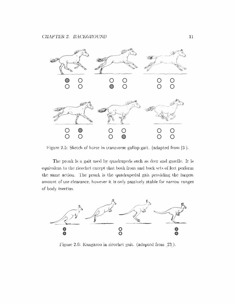
Figure 2.5: Sketch of horse in transverse gallop gait. (adapted from [3]).
The pronk is a gait used by quadrupeds such as deer and gazelle. It is
equivalent to the ricochet except that both front and back sets of feet perform
the same action. The pronk is the quadrupedal gait providing the largest
amount of toe clearance, however it is only passively stable for narrow ranges
of body inertias.
Figure 2.6: Kangaroo in ricochet gait. (adapted from [23]).

CHAPTER 2. BACKGROUND 12
2.2.8 The Bound
The bound is a running gait used by a few small quadrupeds such as squirrels,
rodents, and dogs. In the bound, support alternates between pairs of legs,
with the fore and hind limbs acting in unison to thrust the body forward.
Figure 2.7 shows a Siberian souslik in a bound gait. As can be observed from
this �gure, there is approximately a 180o phase di�erence between the sets
of front and back legs. This gait is of particular interest since, of all gaits
discussed so far, the bound has the shortest gait period, allowing for frequent
interactions of the legs with the ground. This makes the bound well suited for
obstacle avoidance and for providing propulsion [8]. Simulation analysis �rst
conducted by Murphy [21] and later validated by Neishtadt and Li [47] showed
that certain simple planar quadruped bounding models are always passively
stable for dimensionless body inertia values of less than one.
Figure 2.7: Long tailed Siberian souslik in bound gait. (adapted from [14]).
2.3 Control of Legged Robots
Legged robotic systems are divided into two categories : statically and dynam-
ically stable robots, di�ering in the mechanism used to maintain stability.
At low speeds, statically stable robots maintain balance by ensuring that
the ground projection of the centre of mass (COM) of the robot is contained
within the convex polygon formed by the feet in contact with the ground at all
times. McGhee and Frank [43] de�ned the longitudinal stability margin as the
shortest distance between the projected COM location and the convex support

CHAPTER 2. BACKGROUND 13
polygon boundaries (see �gure 2.8). Maintaining the projection of COM inside
the support polygon, ensures that the robot will not topple if there are delays
in motion or if there is a vehicle power failure. To do this, statically stable
robots are typically designed having more than four legs, however statically
stable bipeds with large feet have also been built. To minimise the e�ects
of the destabilising forces resulting from the internal energy of reciprocating
limbs, statically stable robots usually have legs with a low mass as compared
to that of the body.
As the robot's speed begins to increase, the inertia and velocity of a
robot's body starts to make the ground projection of the COM a less accurate
means of assessing robot stability. To address this problem, energy based
stability measures have since been proposed by Messuri and Klein [44] and by
Nagy et al. [46].
Figure 2.8: A low speeds statically stable robots can maintain stability by
keeping the projection of their center of mass, also referred to as the ground
projection of the centre of mass (GCM), within the convex hull formed by the
support feet.
Statically stable robots designed to date include the Ohio State Univer-
sity Active Suspension Vehicle (OSU-ASV) [42], Ambler [4], Dante II [5], and
the SONY Aibo Dog [37] (see �gure 2.9).
Statically stable legged robots locomotion speed is typically limited, de-

CHAPTER 2. BACKGROUND 14
Figure 2.9: SONY Aibo Dog [17].
pending on geometry, to much less than one body length per second. Dynam-
ically stable robots, on the other hand, are not subject to these constraints
and can exploit dynamic forces and feedback to maintain marginal stability
in a limit cycle that repeats once each stride.
Unfortunately, dynamically stable robots su�er from a lack of formal
control development and analysis techniques, since these systems exhibit dis-
continuous dynamics at state transitions, are highly nonlinear, are multi-input
multi-output, act in gravity �elds, and interact with unstructured complex en-
vironments. In addition, benchmarks for such systems also di�er from more
classical measures of performance such as disturbance rejection and command
following. Instead, measures such as biological similarity, locomotion smooth-
ness, eÆciency, top speed, and robustness are often used [35]. To add to these
already signi�cant challenges, controller synthesis can be further complicated
since it is often advantageous to limit or reduce actuated degrees of freedom in
robot design and instead exploit passive elements, such as springs, to provide
compliance.

CHAPTER 2. BACKGROUND 15
To date, no work exists on dynamical walking controller design for un-
deractuated quadruped robots with the exceptions of research in three closely
related areas: control of dynamic running robots, control of dynamic walking
robots with articulated legs, and exploiting passive dynamics in legged robot
control. Section 2.4 summarises key work done to date in these areas.
2.4 Control of Dynamically Stable Legged Robots
2.4.1 Control of Running Robots
Given the lack of formal development and control analysis techniques, the
largest category of control synthesis approaches used to date in legged robotics
has been based on intuition, experimentation, and simulation. Although many
dynamic hopping, jumping, and running robots have been developed, a com-
plete review is outside the scope of this thesis. Instead, key control approaches
for dynamic legged robots will be addressed.
In the area of running robots Raibert [54] performed arguably some
of the most important research to date. Starting with a one legged planar
robot, control of running was investigated. A novel strategy was proposed that
partitioned control of running into three decoupled parts, synchronised by a leg
�nite state machine (�gure 2.10). Control of hopping height, forward speed
and body pitch were treated as three separate control tasks with dynamic
coupling treated as system disturbances. Hopping height was regulated by
specifying the thrust to be delivered by the leg during stance and forward speed
of the robot was controlled by extending the foot to a desired position during
ight. Leg touchdown position was calculated by trying to maintain symmetry
in running (i.e. placing the foot at half the forward distance travelled by the
robot in the previous stride). The third part of the control algorithm applied
a hip torque during stance in order to achieve a desired body angle.
Using �ndings from experiments with the one legged hopper and borrow-

CHAPTER 2. BACKGROUND 16
Figure 2.10: Raibert used a simple three part controller in the control of
his monopod : 1) A thrust was applied to control vertical hopping height
2) Forward speed was regulated by placing the leg at a desired touchdown
position 3) During stance hip torque was applied to achieve a desired body
angle.
ing the concept of virtual legs, originally proposed by Sutherland [59], control
was later generalised for various other robots including a three dimensional
monopod, planar, and three dimensional bipeds, as well as a three dimensional
quadruped robot (�gure 2.11). Use of virtual legs permitted Raibert to ex-
ploit symmetry in certain animal gaits, by grouping legs that acted together
into virtual legs and using the tri-partite algorithm on these virtual legs. This
strategy allowed the Raibert quadruped to pace, trot, pronk, and bound 1 [55].
A more detailed discussion of the virtual leg concept is presented in chapter
5 in the context of the dynamic walking controller developed for this thesis.
To focus e�orts on the task of control and robot design, Raibert elim-
inated power constraints and used powerful hydraulic actuators, driven by
pumps located o� the robot. To improve upon the robot energetics Gregorio
and Buehler [27, 28], designed an electrically actuated version of the Raibert
one-legged hopper called Monopod I (�gure 2.12) that signi�cantly reduced
power consumption. Ahmadi further re�ned Monopod I's design, when it was
1a description of the pace, trot, pronk and bound gaits can be found in section 2.2

CHAPTER 2. BACKGROUND 17
Figure 2.11: MIT Quadruped [54].
observed that 40 % of energy consumption during a stride was consumed by
the hip actuator during the forward leg swing. By exploiting hip compliance
and coordinating the vertical and rotational dynamics of the body, Mono-
pod II (see �gure 2.13) reduced the power consumed during locomotion from
125 W, for Monopod I, to less than 68 W of mechanical power [1, 2]. Both
Monopods I and II used modi�ed versions of the Raibert three part algorithm,
for control of running. Ahmadi also proposed the non-dimensional locomotion
time variable as a alternative means of parametrising locomotion behaviour.
More recently, Papadopoulos and Buehler [48, 49] showed that with a
modi�ed version of the three-part algorithm, simple torque control in stance,
and a quasi-static slip control algorithm, stable pronking and bounding could
be obtained despite a robot design that did not include linear leg actuation.
Experimentation revealed open-loop stability of Scout II in running and proved
robust to disturbances at speeds of up to approximately 1.2 m/s.

CHAPTER 2. BACKGROUND 18
Figure 2.12: ARL Monopod I.
2.4.2 Control of Walking Robots with Articulated Legs
Since most legged robot designs are at least partially inspired by existing
biological systems, it is natural to have develop control approaches for legged
robots having articulated joints. Knees allow robots to more easily avoid
toe stubbing, allowing repeatable cycles of support and leg swinging and to
actively control robot torso height.
In the area of control development for such robots, Dunn and Howe [19,
20] proposed a dynamic bipedal walking controller that constrained touchdown
hip velocity. Forward velocity tracking as well as step length control, two
highly desirable characteristics for planning locomotion through unstructured
environments, were achievable using this approach. Similar biped controls
have also been published in the literature [18].
Virtual Model Control
Motivated by the diÆculties of describing complex motion control tasks and
the lack of formal control techniques for legged robots, Pratt [50, 35] proposed
a control concept, called V irtual Model Control. This technique, which in-
volves a forward kinematic analysis of the system, is based on using simulated
virtual mechanical components, such as imaginary spring damper systems, to

CHAPTER 2. BACKGROUND 19
Figure 2.13: ARL Monopod II.
arti�cially constrain a system's bodies. By calculating the imaginary forces
exerted on the system by the virtual components and by performing the ap-
propriate transformations, torques and forces to command to real actuators
can be calculated.
In addition to having a compact notation, virtual model control bene�ts
from limited computational requirements since many of the key matrices may
be precomputed and optimised. Furthermore, with the exception of parallel
link systems, no matrix inversion is required. Lastly since virtual components
are linearly additive, they may be easily superposed to obtained the combined
e�ect of various virtual components. However, this approach still requires
much control insight and manual parameter tuning in order to achieve the
desired behaviour.
To date, the method has been applied to control several bipedal walking
robots at the MIT Leg Lab including Spring Turkey [35] and Spring Flamingo
[52] (see �gure 2.14). Chew [12] later investigated the application of this
technique to bipedal walking over sloped terrain. The method was also used
in simulation on a hexapod robot that actively balanced an inverted pendulum
on its back while walking using an alternating tripod gait [53]. Figure 2.15
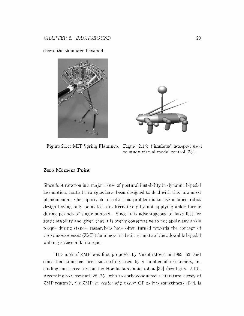
CHAPTER 2. BACKGROUND 20
shows the simulated hexapod.
Figure 2.14: MIT Spring Flamingo. Figure 2.15: Simulated hexapod used
to study virtual model control [53].
Zero Moment Point
Since foot rotation is a major cause of postural instability in dynamic bipedal
locomotion, control strategies have been designed to deal with this unwanted
phenomenon. One approach to solve this problem is to use a biped robot
design having only point feet or alternatively by not applying ankle torque
during periods of single support. Since it is advantageous to have feet for
static stability and given that it is overly conservative to not apply any ankle
torque during stance, researchers have often turned towards the concept of
zero moment point (ZMP) for a more realistic estimate of the allowable bipedal
walking stance ankle torque.
The idea of ZMP was �rst proposed by Vukobratovi�c in 1969 [63] and
since that time has been successfully used by a number of researchers, in-
cluding most recently on the Honda humanoid robot [32] (see �gure 2.16).
According to Goswami [26, 25], who recently conducted a literature survey of
ZMP research, the ZMP, or center of pressure CP as it is sometimes called, is

CHAPTER 2. BACKGROUND 21
best de�ned as the point on the ground where the resultant ground reaction
force actually acts. If the ZMP coincides with the location of the resultant
force generated from the inertia and static gravitational forces acting on the
system, there will be no moment acting on the body in the transverse direc-
tion. In reality the term ZMP is a misnomer, since only two of the three
moment components tend to be zero, if the ZMP coincides with the point of
action of the resultant body force. A moment is still usually produced by
tangential ground friction forces acting about the central axis of the body.
Figure 2.16: Honda humanoid robot [32].
The ZMP should not be confused with the ground projection of the center
of mass (GCM) used in determining the stability margin of statically stable
robots as mentioned in section 2. Figure 2.17 shows a simpli�ed robot rep-
resented as a point mass supported by an actuated ankle. The left image of
�gure 2.17, shows the point mass hanging far to the right of the foot causing
the GCM to lie outside the sole's area of support. If a torque is applied to
counteract the static imbalance, the robot's ankle will rotate, e�ectively plac-
ing the ZMP at the toes. However, if the point mass is accelerated forward, as
is the case of the right hand image of �gure 2.17, the resultant force generated
by the inertia and gravitational forces will place the ZMP under the foot thus
avoiding tipping. A similar strategy of accelerating the heavy upper body of
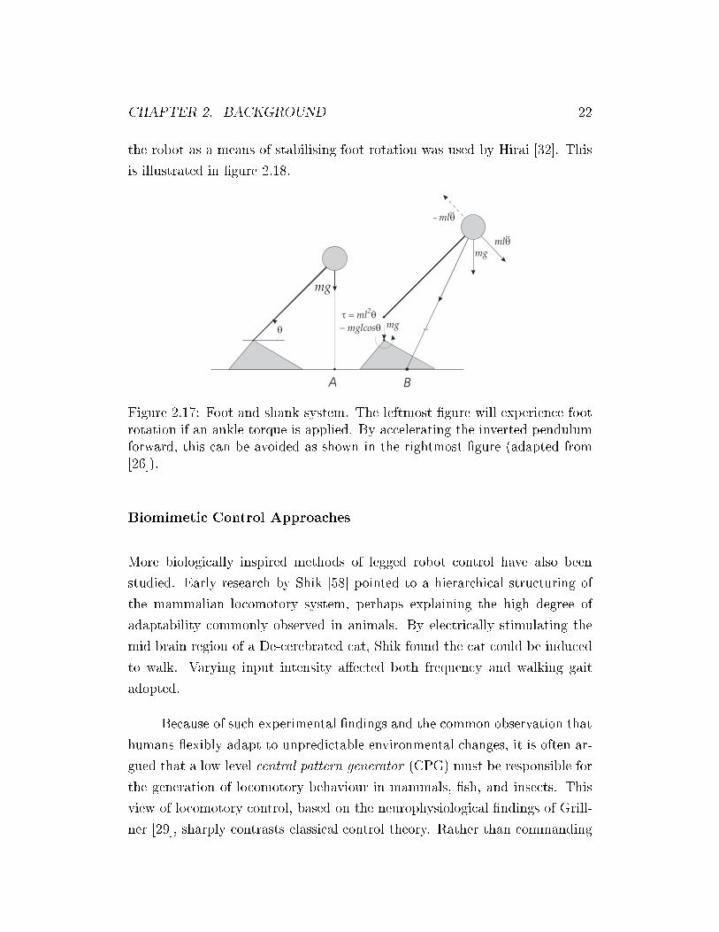
CHAPTER 2. BACKGROUND 22
the robot as a means of stabilising foot rotation was used by Hirai [32]. This
is illustrated in �gure 2.18.
Figure 2.17: Foot and shank system. The leftmost �gure will experience foot
rotation if an ankle torque is applied. By accelerating the inverted pendulum
forward, this can be avoided as shown in the rightmost �gure (adapted from
[26]).
Biomimetic Control Approaches
More biologically inspired methods of legged robot control have also been
studied. Early research by Shik [58] pointed to a hierarchical structuring of
the mammalian locomotory system, perhaps explaining the high degree of
adaptability commonly observed in animals. By electrically stimulating the
mid brain region of a De-cerebrated cat, Shik found the cat could be induced
to walk. Varying input intensity a�ected both frequency and walking gait
adopted.
Because of such experimental �ndings and the common observation that
humans exibly adapt to unpredictable environmental changes, it is often ar-
gued that a low level central pattern generator (CPG) must be responsible for
the generation of locomotory behaviour in mammals, �sh, and insects. This
view of locomotory control, based on the neurophysiological �ndings of Grill-
ner [29], sharply contrasts classical control theory. Rather than commanding

CHAPTER 2. BACKGROUND 23
Figure 2.18: Planar biped model showing ZMP. By accelerating the heavy
upper body, the resultant inertia and gravity force acts under the foot. If this
point coincides with the ZMP moment will be induced on the robot's ankle
(adapted from [32]).
joint trajectories and relying on feedback to provide real-time adaptability to
the system against disturbances and errors, CPG based methods rely on the
emergent behaviour stemming from interactions between the rhythmic activ-
ities of the neural system, the musculo-skeletal system, and the environment.
The use of a hierarchical approach is also found in the work of Brooks [9], in
the arti�cial intelligence community, who obtained complex robot behaviour
using a layered subsumption architecture.
A commonly used CPG, based on modeling the neural physiological sys-
tem of animals is the neural oscillator (NO). A NO consists of a network of
neurons connected in such a way that one neuron's excitation suppresses that
of the others. Due to these inhibitory connections, torques are induced in al-
ternating directions corresponding to muscle exion and extension. Although
other neuronal network representations exist, the model proposed by Mat-
suoka [39] is often used in the context of biomimetic robot control. Equation
2.1 shows the mentioned model and an illustration is provided in �gure 2.19.

CHAPTER 2. BACKGROUND 24
In equation 2.1, ui is membrane potential of the neuron body, � is a time
constant determining the rise time for a step input, � determines the steady
state �ring rate for a constant input, vi is the adaptation variable, �0 is a time
constant specifying the time lag before adaptation takes e�ect, and yi is the
neuron output. Feedback is also incorporated into the neural oscillator model,
as can be seen from the presence of a feedback term in equation 2.1.
� _ui = �ui � �vi + u0 + Feedbacki +
nXj=1
!ijyj
�0 _vi = �vi + yi (2.1)
yi = max(0; ui)
Figure 2.19: Neural oscillator model (adapted from [30]).
In addition to being the �rst neuronal network model to incorporate
adaptation, the Matsuoka's model is of particular interest since it has been
used by Taga [61, 60] to obtain planar bipedal walking in simulation and
more recently by Kimura [30, 36] to obtain experimental walking and running
results in a quadruped robot, Patrush. Kimura also added other biologically
inspired layers to his walking controller.

CHAPTER 2. BACKGROUND 25
Although NO methods of locomotion control are appealing because they
aim to model nature, they are not without shortcomings. Firstly, our under-
standing of the mammalian neurophysiology is still limited, as is our knowl-
edge of the neuronal circuits making up these organisms. This poses some
signi�cant problems since NO output varies signi�cantly depending both on
the number and weight of connections. Furthermore, given the strong in-
terconnection in typical NO circuits, additional connections increase the pa-
rameter space exponentially, making the incremental addition of complexity
prohibitive. NO output is also highly sensitive to parameter variations, with
small modi�cations producing signi�cantly di�erent output. Although certain
parameters are attributed with playing di�erent roles in shaping output, con-
siderable interdependency still exists. Since the parameter space is extremely
large to begin, NO circuit tuning can easily become intractable. Lastly, the
feedback mechanisms used by living organisms is still unknown, making the
choice of a feedback expression for equation 2.1 somewhat arbitrary. Taga and
Kimura both used knee joint angle as feedback in the hip NO.
2.4.3 Passive Dynamics in Legged Robot Control
Another area of research in legged robotics, is the study of mechanism design
as a means of reducing mechanical complexity and energy consumption. By
replacing motors with passive joints or springs, equivalent motions can be
obtained without added power requirements. From a controls point of view
this approach makes a lot of sense; If the passive (unforced) system response
can be used as much as possible, required control actions can be minimised
thereby reducing power consumption and potentially simplifying control.
The seminal work in this area was done by McGeer [40] who built a
series of bipeds capable of walking passively down shallow inclines powered
only by gravity. McGeer �rst studied a biped with rigid legs that used active
foot retraction to ensure the swing foot cleared the ground (see �gure 2.20).
Subsequently, he conducted a parametric study of various physical parameters
such as foot radius, leg inertia, center of mass location, and hip mass to

CHAPTER 2. BACKGROUND 26
determine their impact on walking. This work was later followed by the study
of a experimental biped having passive knees [41]. These mechanisms were
shown to be passively stable and robust to minor perturbations. Garcia,
Chatterjee, and Ruina [24] later expanded upon McGeer's analytical �ndings,
stating necessary conditions for optimal walking eÆciency.
Figure 2.20: McGeer's gravity powered passive walker without knees [40].
The ideas proposed by McGeer have also been used as the basis of control
for legged robots with actuated joints. In this area, Pratt [51] reversed the
knees of the spring amingo biped (see �gure 2.14) to allow the knee joint to
act almost entirely passively during swing thus signi�cantly reducing energy
consumption. Hawker amd Buehler [31] applied a similar strategy to control
the lower leg motion of a version of the Scout II quadruped with knees. The leg
design used a completely passive knee that could be locked/unlocked using a
solenoid. This approach, permitted planar quadrupedal trotting. To eliminate
roll instabilities resulting from the planar leg design, the robot was constrained
to only move in the saggital plane.
Related research has focused on exploiting robot design to passively sta-
bilise running of legged robots. Ringrose [57] showed that using (roughly)
semi-circular feet for a series of monopods, bipeds, and quadrupeds stable dy-
namic running could be achieved without any sensory feedback. His �ndings

CHAPTER 2. BACKGROUND 27
suggested that it would be possible to build robots containing no sensors, by
carefully designing the robot's mechanical system.
Similarly, Buehler, Cocosco and Yamazaki [10, 11] showed that using
a simple robot design having only one actuated degree of freedom per joint,
stable open-loop walking, turning, and step climbing could be achieved despite
using only limited feedback. Their Scout I and Scout II robots, used sti� stick
legs and relied on momentum transfer to maintain regular body pitching. A
simple ramp controller was proposed that used a four state state-machine,
based on the overall robot state, to coordinate locomotion activities. These
four phases were 1) Front support, 2) Front to back double support, 3) Back
support, 4) Back to Front double support. Figure 2.21 shows Scout II (with
sti� legs) in these four phases of motion.
Figure 2.21: Scout II walking with sti� legs. Images are read left to right, top
to bottom.
Figure 2.22 shows the devised ramp control. As illustrated, when the
robot entered the back leg support state, the back legs were swept at a constant
rate _�2, between a �xed touchdown angle �2 start, until the front legs entered a

CHAPTER 2. BACKGROUND 28
support phase. Here � is the leg angle with respect to the body. The legs were
then kept at a their touchdown position �2 end for a �xed period of time, before
being retracted back to their touchdown position. Throughout this process,
the front legs where kept \locked" at a perpendicular position with respect to
the body.
The ramp controller was open loop and only needed to know if the
legs were in contact with the ground. Thus since only limited proprioceptive
sensing was required for the controller it was extremely straightforward to
implement. Using numerical analysis of Scout's equations of motion, Cocosco
[13] showed a nearly global domain of stability for the controller, even though
no active stabilisation was being used.
Although the controller showed a great deal of promise and was very suc-
cessful on Scout I, leg impacts during sti� legged walking were quite signi�cant
on Scout II. These large impulsive forces resulted in undesirable stressing of
the robots mechanical system and in lossy dynamics. These factors motivated
the use of compliant legs on Scout. It was believed that adding compliance in
the legs, would also permit previously unrealisable running gaits such as the
bound.

CHAPTER 2. BACKGROUND 29
6
-
�2
time
@@@@@@@@@@@ �
����������
�2 start
�2 end
_�2
Back LegSupport
Front LegSupport
-� -�tstart tretract
Figure 2.22: Ramp controller input for �2 for one complete step.
2.5 Summary
This chapter presented an overview of animal gaits aimed at familiarising the
reader with relevant terminology needed in future discussion. Although no
work exists on dynamic walking controller design for underactuated quadruped
robots, research was described in three closely related areas: control of dy-
namic running robots, control of dynamic walking robots with articulated legs,
and exploiting passive dynamics in legged robot control.

Chapter 3
Scout II
3.1 Overview
This chapter describes the Scout II robot, for which the control algorithms
discussed in thesis were developed. Mechanical, electrical, and software spec-
i�cations for the system are discussed. In addition, motivation and design
decisions used in the redesign of Scout's electrical and software systems are
described.
3.2 Platform Speci�cations
The locomotion algorithms developed for this thesis, were designed for the
Scout II robot. Scout II is a quadruped robot developed at McGill University's
Ambulatory Robotics Lab (ARL) by Robert Battaglia [6] with the aim of
investigating the feasibility and trade-o�s of underactuation in legged robots.
30

CHAPTER 3. SCOUT II 31
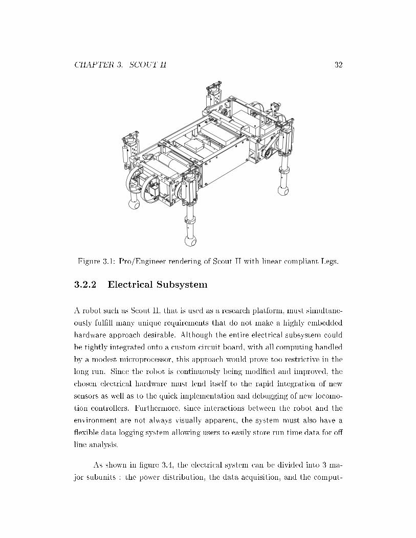
3.2.1 Mechanical Subsystem
Each of Scout II's legs has one actuated rotational hip joint and a passive pris-
matic joint. The prismatic legs joints can be locked for sti� legged operation
or used in a compliant mode. When used in the compliant mode, the leg de-
sign can accommodate a wide range of springs, allowing the system dynamics
to be tailored to the desired response. Similarly, the robot's leg length can
also be modi�ed using various leg extenders. Figures 3.1 - 3.3 show pictures
of Scout II. For clarity, relevant robot parameters have been summarised in
table 3.1.
All experiments documented in this thesis used two springs on each of
Scout's legs to obtain the desired leg sti�ness. This resulted in a leg spring
sti�ness of approximately 2250 N/m. This leg sti�ness was chosen experi-
mentally since lower spring constants produced sluggish or undesirable body
behaviour. The chosen spring combination also allowed a single leg con�gura-
tion to be used for both running and bounding. A detailed description of the
springs used during experiments is provided in table 3.2. For simplicity, the
robot leg length was not altered.
Since Scout II was designed to operate without a tether in unstructured
urban environments, all computing, sensing, and power subsystems are con-
tained on board the robot. To date, the mechanical design has proven quite
rugged and has endured considerable abuse from continuous experimentation.
Unfortunately the electrical subsystem did not show the same resilience and
thus a complete redesign of this system was undertaken as part of this thesis.
Furthermore, since considerable coupling existed between the electrical system
and the implementation of the real-time software architecture used to con-
trol the robot, the software subsystem was also redesigned and implemented.
Sections 3.2.2 and 3.2.3 describe design considerations and implementation
decisions taken as part of this process.
CHAPTER 3. SCOUT II 32
Figure 3.1: Pro/Engineer rendering of Scout II with linear compliant Legs.
3.2.2 Electrical Subsystem
A robot such as Scout II, that is used as a research platform, must simultane-
ously ful�ll many unique requirements that do not make a highly embedded
hardware approach desirable. Although the entire electrical subsystem could
be tightly integrated onto a custom circuit board, with all computing handled
by a modest microprocessor, this approach would prove too restrictive in the
long run. Since the robot is continuously being modi�ed and improved, the
chosen electrical hardware must lend itself to the rapid integration of new
sensors as well as to the quick implementation and debugging of new locomo-
tion controllers. Furthermore, since interactions between the robot and the
environment are not always visually apparent, the system must also have a
exible data logging system allowing users to easily store run time data for o�
line analysis.
As shown in �gure 3.4, the electrical system can be divided into 3 ma-
jor subunits : the power distribution, the data acquisition, and the comput-

CHAPTER 3. SCOUT II 33
Figure 3.2: Scout II with linear compliant legs
ing/control subsystems.
The �rst iteration of Scout II's electrical system used a custom data
acquisition system developed at ARL by Nadim El-Fata called the Standard
Parallel Port/Serial Peripheral Interface (SPP/SPI) system. The SPP/SPI
system is a distributed data acquisition system that uses the computer's par-
allel port and the serial peripheral interface (SPI) communications standard
to perform input/output (I/O) with up to 8 input and 8 output custom data
modules at rates of up to 1 kHz. At the heart of the SPP/SPI was a multiplexer
board that plugged into the computer's parallel port and interfaced to various
I/O modules. This multiplexer had telephone style connectors allowing users
to rapidly customise the system to their particular sensing requirements. Fig-
ure 3.5 shows a photograph of the SPP/SPI system as it used to be mounted
on Scout. Scout II used two SPP/SPIs.
Although use of the SPP/SPI was extremely successful on Scout I [64],
since the robot used only limited sensing, it did not scale well to the larger
Scout II robot. Because of its distributed architecture, a system such as the
SPP/SPI signi�cantly increased the amount of cabling on the robot, leading
to frequent loosening and breaking of cables. In addition, the added power re-

CHAPTER 3. SCOUT II 34
Table 3.1: Scout II mechanical speci�cations [6]. * The reported overall robot
mass was calculated after the electrical system redesign.
Parameter Value
Body length 0.837 m
Body height 0.126 m
Front hip width 0.498 m
Rear hip width 0.413 m
Hip-to-hip length 0.552 m
Total mass� 25.545 kg
Body mass 21.865 kg
Body Inertia from COM about
pitch axis 1.091 kgm2
roll axis 0.161 kgm2
Leg length 0.255-0.457 m
Leg mass 0.920 kg
Leg inertia (about hip) Length (mm) Inertia (g mm2)
255.9 12.94
275.0 14.27
294.1 16.26
313.2 18.90
332.3 22.19
quirements resulting from distributing computing to individual data modules,
proved to be ill suited for a mobile robot such as Scout II.
The mentioned shortcomings of the SPP/SPI motivated a shift to a
centralised data acquisition system using standard o� the shelf components,
capable of meeting Scout's present and future needs. Given the need to change
the data acquisition system, the opportunity was also taken to upgrade the
robot's computer. A discussion of the chosen architecture and of the designed
custom electronics follows.
CHAPTER 3. SCOUT II 35
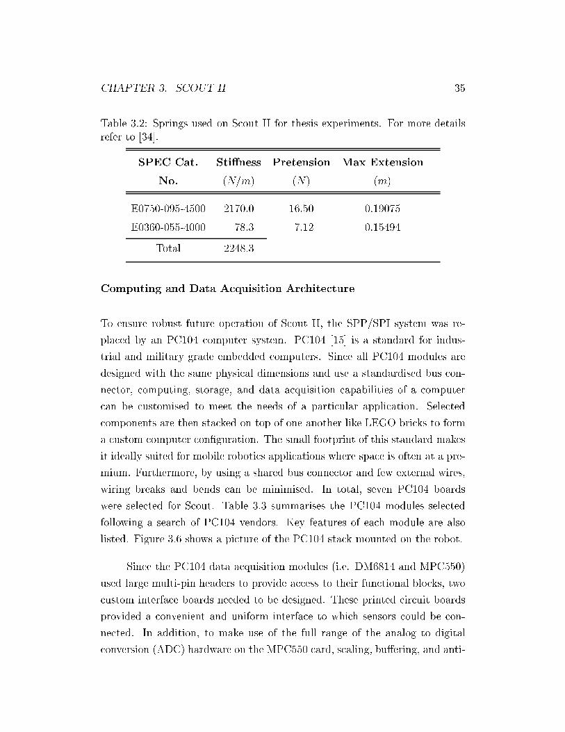
Table 3.2: Springs used on Scout II for thesis experiments. For more details
refer to [34].
SPEC Cat. Sti�ness Pretension Max Extension
No. (N=m) (N) (m)
E0750-095-4500 2170.0 16.50 0.19075
E0360-055-4000 78.3 7.12 0.15494
Total 2248.3
Computing and Data Acquisition Architecture
To ensure robust future operation of Scout II, the SPP/SPI system was re-
placed by an PC104 computer system. PC104 [15] is a standard for indus-
trial and military grade embedded computers. Since all PC104 modules are
designed with the same physical dimensions and use a standardised bus con-
nector, computing, storage, and data acquisition capabilities of a computer
can be customised to meet the needs of a particular application. Selected
components are then stacked on top of one another like LEGO bricks to form
a custom computer con�guration. The small footprint of this standard makes
it ideally suited for mobile robotics applications where space is often at a pre-
mium. Furthermore, by using a shared bus connector and few external wires,
wiring breaks and bends can be minimised. In total, seven PC104 boards
were selected for Scout. Table 3.3 summarises the PC104 modules selected
following a search of PC104 vendors. Key features of each module are also
listed. Figure 3.6 shows a picture of the PC104 stack mounted on the robot.
Since the PC104 data acquisition modules (i.e. DM6814 and MPC550)
used large multi-pin headers to provide access to their functional blocks, two
custom interface boards needed to be designed. These printed circuit boards
provided a convenient and uniform interface to which sensors could be con-
nected. In addition, to make use of the full range of the analog to digital
conversion (ADC) hardware on the MPC550 card, scaling, bu�ering, and anti-

CHAPTER 3. SCOUT II 36
aliasing circuitry needed to be designed. Table 3.4 summarises Scout's I/O
needs, classifying items according to the required type of I/O. Appendix A
contains all the schematics for the designed custom hardware.
3.2.3 Software Subsystem
Previous designs and implementations of the software subsystem for Scout did
little to abstract out speci�cs of the hardware operation from the state based
runtime robot code. In addition, the software subsystem, which was mainly
legacy code from previous projects, contained many inconsistencies. These
and other points strongly motivated a redesign of the software subsystem to
limit coupling and to improve overall system performance.
Although the data logging system from the original Scout code was main-
tained, given its ease of use, the remainder of the code was revised to eliminate
all assumptions regarding the data acquisition hardware. By abstracting out
the speci�cs of the low-level hardware it was ensured that future modi�cations
of Scout's physical hardware would not interfere with the higher level state
based control code.
Control Code Architecture
As in the past, Scout II used the QNX realtime operating system (OS) [38].
QNX is a POSIX compliant multi-process, multi-user UNIX avoured real-
time OS. Although QNX supports multiple processor, and uses a preemptive
priority based scheduler to ensure all processes are properly serviced, the ker-
nel is not thread safe. Therefore, although multiple processes can be run,
users must resort to interprocess communication or message passing schemes
to allow processes to share information. Since interprocess communication
can be a costly approach to sharing data, degrading performance, the code
was instead designed using a simple polling scheme. Using this scheme, data
was gathered, computation was performed, to determine state variables, and
CHAPTER 3. SCOUT II 37
output commands were sent to the actuators at each execution loop.
To modularise some additional functionality, a few blocking processes
were implemented that took care of some low bandwidth activities, such as
waiting for instructions from a TV remote infrared module that was connected
to one of the computer's serial ports. This allowed users of the robot to send
high-level instructions or to dynamically vary parameters during experiments.

CHAPTER 3. SCOUT II 38
Figure 3.3: Top and side Pro/Engineer isometric views of Scout II.

CHAPTER 3. SCOUT II 39
Figure 3.4: Electrical system block diagram. This system can be subdivided
into three main subsystems : power distribution, computing and data acqui-
sition.
Figure 3.5: Underside of Scout, showing SPP/SPI multiplexers and connected
data I/O modules.

CHAPTER 3. SCOUT II 40
Figure 3.6: PC104 computer mounted inside robot chassis. Designed custom
I/O boards can be seen on left hand side of image.

CHAPTER 3. SCOUT II 41
Table 3.3: PC104 modules selected for Scout II following web search of hard-
ware vendors
Part No. Quantity Description/Features
CMW6686GX233-64/DO16 1 - Pentium 233 MHz CPU Module
- SVGA controller
- 2 RS232 serial ports
- 1 ECP/EPP parallel port
- Keyboard interface
- 64 MB RAM with 16 MB Flash Disk
EPWR104 1 - 50W Power Supply Module.
- Input Range : 8-40 VDC
- Output Range : +5 VDC @ 5 A
+12 VDC @ 2 A
�12 VDC @ 0.5 A
CM202 1 - PC104 Networking Module
- NE-2000 Ethernet with AUI
- 10Base-T and 10Base-2 interfaces
CMT107 1 - 6GB IDE Hard drive Module
- IDE Controller and slave connector
DM6814 2 - 3 16-bit incremental encoder channels
- Digital (6 bi-directional, 12 input)
- 3 16-bit counter/timers (8 MHz)
MPC550 1 - 16 12-bit analog inputs
- 24 digital I/O lines
- 8 12-bit analog output channels
- 3 16-bit counter/timers (7 MHz)

CHAPTER 3. SCOUT II 42
Table 3.4: Scout II I/O requirements
Direction Type Quantity
INPUTS ANALOG
Leg Pots 4
Lasers 2
Gyroscopes 1
Battery Voltage 112
Battery Current 1
Applied Torque 4
DIGITAL
Hall E�ect Sensors 4 4
HCTL
Optical Encoders 4 4
Total 20
OUTPUTS ANALOG
Commanded Torque 8 8
DIGITAL
Watchdog 1 1
PWM
Servos 2 2
Total 11

CHAPTER 3. SCOUT II 43
3.3 Summary
This chapter presented a description of the experimental hardware platform,
the Scout II robot, for which locomotion algorithms were developed. An
overview of key robot subsystems and of design decisions used in the overhaul
of the robot's electrical system was also presented. Lastly software design and
implementation issues relating to the robot's realtime control code were also
addressed.

Chapter 4
Modeling
4.1 Overview
A review of currently available locomotion controller design tools for highly
non-linear and underactuated systems such as Scout II reveals that no ade-
quate theory or techniques exist at this time. Therefore, the synthesis of new
locomotion controllers relies principally on the development of intuition, by
the controller's designer, about system behaviour and dynamics. To help in
developing this intuition, we have found that an iterative process of simulation
and analysis is a good approach.
This section presents modeling and simulation results used to investigate
walking. It was hoped that by using simulation, intuition could be developed
to help guide the design of a walking controller. To begin, a rocking controller
was designed and simulated, that excited the body at its natural frequency
and repeatedly lifted fore and hind legs o� the ground. This controller proved
robust to large variations in parameters even though it was completely open
loop. Next, the rocking controller was modi�ed to obtain stable open loop
walking. Minor modi�cation to the walking algorithm allowed open-loop ve-
locity tracking.
44

CHAPTER 4. MODELING 45
4.2 Simulation Package
To perform the simulations for this thesis, the Knowledge Revolution Work-
ing Model 2D (WM2D) package was used [56]. WM2D, a graphical physics
simulator, allows the simulation of multiply linked planar rigid bodies under
a number of user speci�ed constraints and inputs.
One of the big advantages of using a package such as WM2D is that it
does not require the derivation of the system equations of motion. Instead, sys-
tems can be interactively built and simulated, using a straightforward object-
oriented scripting language. WM2D uses a �fth order Runge-Kutta integrator
that numerically integrates the e�ects of all the forces acting on the bodies
being simulated, yielding accelerations, velocities, and position information.
As with any numerical technique, small errors can add up over time, produc-
ing incorrect results, therefore, an adaptive time step is used by the program
to bound errors at each time interval.
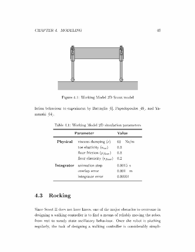
Using this package, a simulation model of Scout II was constructed hav-
ing the same geometric and mass/inertia parameters as the real robot (see
table 3.1). Figure 4.1 shows this model. The constructed model consisted of
seven rigid bodies: top and bottom leg sections and a circular toe for each
leg, as well as a main torso. To model the robot's passive prismatic leg joint,
the top leg section was constrained to move along a frictionless slot placed
in the lower leg. A spring/damper system was also connected between these
bodies to provide the correct compliance. Each leg was then attached to the
main torso via a torque mode actuator. To prevent excessive spring extensions
and to properly model Scout's real legs, two ideal ropes (i.e. no stretch) were
also connected between top and bottom leg sections. The ropes modeled leg
clamps on the robot that limited leg compression.
In addition to physical parameters obtained directly from the robot,
certain other parameters had to be estimated. These values are summarised
in table 4.1. Some of these parameters such as viscous damping c and oor
Coulomb friction �floor were selected based on prior attempts to match simu-
CHAPTER 4. MODELING 46
Figure 4.1: Working Model 2D Scout model
lation behaviour to experiment by Battaglia [6], Papadopoulos [48], and Ya-
mazaki [64].
Table 4.1: Working Model 2D simulation parameters
Parameter Value
Physical viscous damping (c) 60 Ns/m
toe elasticity (�toe) 0.8
oor friction (�floor) 0.8
oor elasticity (�floor) 0.2
Integrator animation step 0.0015 s
overlap error 0.001 m
integrator error 0.00001
4.3 Rocking
Since Scout II does not have knees, one of the major obstacles to overcome in
designing a walking controller is to �nd a means of reliably moving the robot
from rest to steady state oscillatory behaviour. Once the robot is pitching
regularly, the task of designing a walking controller is considerably simpli-

CHAPTER 4. MODELING 47
�ed, since the system will have a tendency to passively maintain this rocking
motion.
When the robot is at rest, there is a 0o phase di�erence between the
front and back sets of legs. This is also true in rocking, with the additional
characteristic that legs also alternate repeatably between stance and ight.
Therefore, rocking was �rst studied as a means of providing a reliable startup
sequence for a robot walking algorithm. It was envisioned that by having
alternating periods of stance and ight at regular intervals that the rocking
controller could later be modi�ed to produce a stable walking gait. A similar
strategy was used by Kimura [30] to excite Patrush, a quadruped robot with
knees, from rest to a running bound, via an intermediate hopping state.
4.3.1 Rocking Model
To study the natural dynamical behaviour of the robot, a simpli�ed planar
two-dimensional robot model was derived and analysed. Figure 4.2 shows
this model. Scout II is modeled as a planar spring mass damper system with
massless legs.
Instead of lumping the robot's overall mass at the geometric center of
the torso, the presented model split the overall mass into two point masses
(each having half the robots mass) located at a distance r (i.e. the radius of
gyration) from the center of the body. According to Beer and Johnston [7],
the radius of gyration is the distance at which the mass of a body should be
concentrated if its moment of inertia with respect to some rotational axis is
to remain unchanged.
r =
sI
M=2=
r1:091
12:5m = 0:295m (4.1)
Equation 4.1 shows the calculated value for the radius of gyration based
on Scout II's current physical parameters. This value is very close to the value
CHAPTER 4. MODELING 48
�
kckc
rd
m
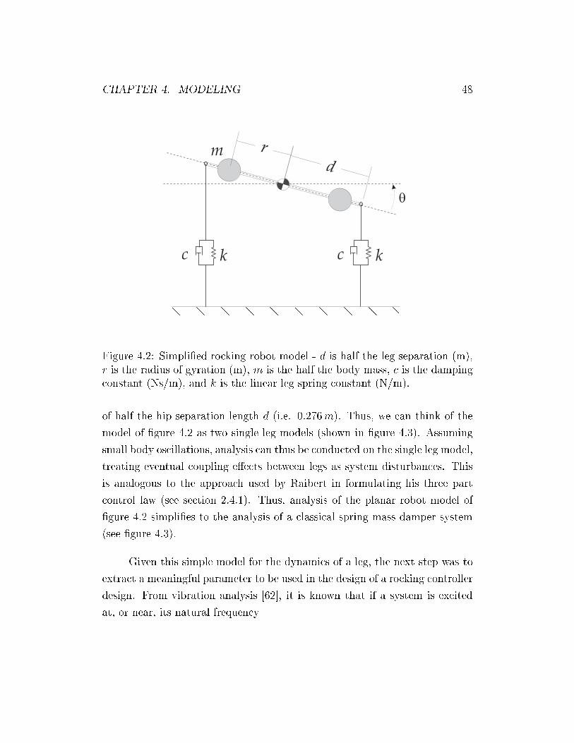
Figure 4.2: Simpli�ed rocking robot model - d is half the leg separation (m),
r is the radius of gyration (m), m is the half the body mass, c is the damping
constant (Ns/m), and k is the linear leg spring constant (N/m).
of half the hip separation length d (i.e. 0:276m). Thus, we can think of the
model of �gure 4.2 as two single leg models (shown in �gure 4.3). Assuming
small body oscillations, analysis can thus be conducted on the single leg model,
treating eventual coupling e�ects between legs as system disturbances. This
is analogous to the approach used by Raibert in formulating his three part
control law (see section 2.4.1). Thus, analysis of the planar robot model of
�gure 4.2 simpli�es to the analysis of a classical spring mass damper system
(see �gure 4.3).
Given this simple model for the dynamics of a leg, the next step was to
extract a meaningful parameter to be used in the design of a rocking controller
design. From vibration analysis [62], it is known that if a system is excited
at, or near, its natural frequency

CHAPTER 4. MODELING 49
m
yc k
Figure 4.3: Single leg robot model - m is half the total robot mass (kg), y is
the height of the point mass measured from the ground at a particular instant
of time, k is the linear leg spring constant, and c is the damping constant.
!n =
rk
m=
r3050
12:5rad=s = 15:6 rad=s (4.2)
it will begin to resonate. Considering damping, the resonant frequency
is
!d = !n
p1� �2 = !n
s1�
�c
2pk m
�2
(4.3)
= 15:6
s1�
�60
2p3050 : 12:5
�2
rad=s = 15:23 rad=s
Although the spring sti�ness value used in the above equations is less
than the sti�ness of springs later selected for the real robot (see section 3.2.1),
these value were originally chosen since they yielded the lowest body rotational
frequency while still allowing repeatable steady state rocking.
Using the above calculated natural frequency, a simple rocking controller
was devised, that excited the system at this frequency. This controller and
results from simulations of the controller are discussed in section 4.3.2.
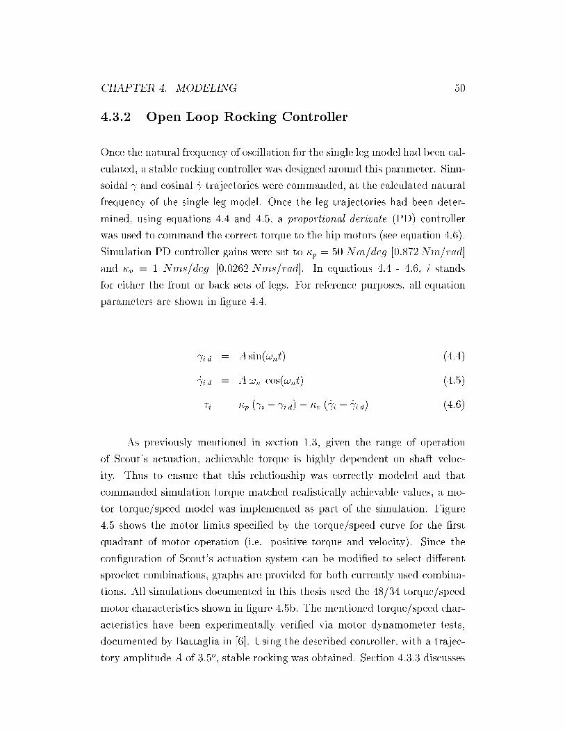
CHAPTER 4. MODELING 50
4.3.2 Open Loop Rocking Controller
Once the natural frequency of oscillation for the single leg model had been cal-
culated, a stable rocking controller was designed around this parameter. Sinu-
soidal and cosinal _ trajectories were commanded, at the calculated natural
frequency of the single leg model. Once the leg trajectories had been deter-
mined, using equations 4.4 and 4.5, a proportional derivate (PD) controller
was used to command the correct torque to the hip motors (see equation 4.6).
Simulation PD controller gains were set to �p = 50 Nm=deg [0:872Nm=rad]
and �v = 1 Nms=deg [0:0262 Nms=rad]. In equations 4.4 - 4.6, i stands
for either the front or back sets of legs. For reference purposes, all equation
parameters are shown in �gure 4.4.
i d = A sin(!nt) (4.4)
_ i d = A !n cos(!nt) (4.5)
�i = �p ( i � i d)� �v ( _ i � _ i d) (4.6)
As previously mentioned in section 1.3, given the range of operation
of Scout's actuation, achievable torque is highly dependent on shaft veloc-
ity. Thus to ensure that this relationship was correctly modeled and that
commanded simulation torque matched realistically achievable values, a mo-
tor torque/speed model was implemented as part of the simulation. Figure
4.5 shows the motor limits speci�ed by the torque/speed curve for the �rst
quadrant of motor operation (i.e. positive torque and velocity). Since the
con�guration of Scout's actuation system can be modi�ed to select di�erent
sprocket combinations, graphs are provided for both currently used combina-
tions. All simulations documented in this thesis used the 48/34 torque/speed
motor characteristics shown in �gure 4.5b. The mentioned torque/speed char-
acteristics have been experimentally veri�ed via motor dynamometer tests,
documented by Battaglia in [6]. Using the described controller, with a trajec-
tory amplitude A of 3:5o, stable rocking was obtained. Section 4.3.3 discusses
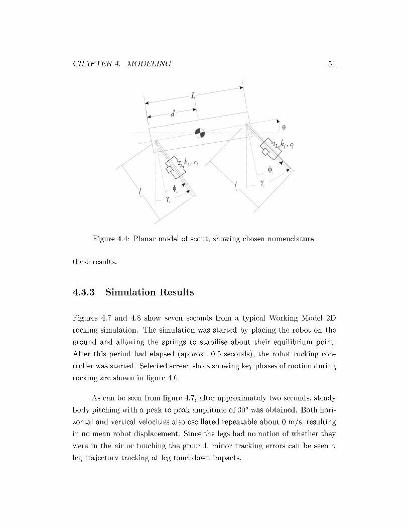
CHAPTER 4. MODELING 51
Figure 4.4: Planar model of scout, showing chosen nomenclature.
these results.
4.3.3 Simulation Results
Figures 4.7 and 4.8 show seven seconds from a typical Working Model 2D
rocking simulation. The simulation was started by placing the robot on the
ground and allowing the springs to stabilise about their equilibrium point.
After this period had elapsed (approx. 0.5 seconds), the robot rocking con-
troller was started. Selected screen shots showing key phases of motion during
rocking are shown in �gure 4.6.
As can be seen from �gure 4.7, after approximately two seconds, steady
body pitching with a peak to peak amplitude of 30o was obtained. Both hori-
zontal and vertical velocities also oscillated repeatable about 0 m/s, resulting
in no mean robot displacement. Since the legs had no notion of whether they
were in the air or touching the ground, minor tracking errors can be seen
leg trajectory tracking at leg touchdown impacts.

CHAPTER 4. MODELING 52
Figure 4.5: First quadrant torque/speed relationship for Scout II's current
actuation system. The presented curves assume a) 48/28 sprocket combination
b) 48/34 sprocket combination (Assumed eÆciencies : �gearhead = 68 % and
�belt = 96 %). Figure adapted from [6].
Figure 4.9 shows the implemented torque/speed model for all four quad-
rants of motor operation. Applied torque is also plotted on top of this graph.
As can be observed, the output motor torque is clipped to stay within the
speci�ed polygon.
4.3.4 Parameter Sensitivity
To study the robustness and sensitivity of the open loop rocking controller,
simulations where repeated for variations in controller and robot model pa-
rameters.
Since the oscillation amplitude of equation 4.4 is the only user speci�ed
controller parameter, this value was �rst modi�ed. Thus, a set of simulations
was performed for which the leg oscillation amplitude was increased in 5o
increments from 5o to 25o. Rocking became unstable for oscillation amplitudes
exceeding 15o. This e�ect is not entirely surprising given that the simple single
leg model used to derive the controller did not take into account deviations of
the leg from the perpendicular.

CHAPTER 4. MODELING 53
Figure 4.6: Working Model 2D rocking simulation screen shots
Next, physical robot parameters were modi�ed to see what e�ect model-
ing inaccuracies would have on eventual rocking on the real robot. To begin,
the e�ect of shifting the body's center of mass (COM) was investigated. To
do this, a set of simulations was run for which the COM was shifted in 0.05
m increments towards the front of the robot. The results obtained from these
experiments were very promising. Although decreased front foot clearance
was observed, simulations showed that for o�sets of less than or equal to 0.1
m that the open loop controller still yielded stable rocking. This is quite im-
pressive since a 0.1 m shift in the COM represents about 20 % of the robot's
body length. This showed that a large mass imbalance would have to exist in
the robot to prevent rocking from working.
Next, linear spring sti�ness (i.e. k) was varied � 50% for the front leg.
Surprisingly stable rocking was observed for changes in spring sti�ness of up
to � 40%. Changes of spring sti�ness greater than 40% resulted in no lifto�
of the back leg. Increases of the spring constant also shows large backward
motion of the body.

CHAPTER 4. MODELING 54
1 2 3 4 5 6 7−20
−10
0
10
20a)
1 2 3 4 5 6 70.26
0.28
0.3
0.32
0.34b)
1 2 3 4 5 6 7−0.5
0
0.5c)
1 2 3 4 5 6 7−0.5
0
0.5d)
t (s)
�(deg)
y(m)
_x(m=s)
_y(m=s)
Figure 4.7: Torso behaviour for rocking simulation. a) Body pitch � (deg.),
b) Body height y (m), c) Horizontal velocity _x (m/s), d) Vertical velocity _y
(m/s).
Once rocking had been investigated, modi�cations to the rocking algo-
rithm were studied to obtain compliant walking.

CHAPTER 4. MODELING 55
4 5 6−5
0
5a)
γ 1 (de
g.)
t (s)4 5 6
−5
0
5b)
γ 2 (de
g.)
t (s)
Figure 4.8: Actual (solid) and desired (dotted) leg (deg.) trajectories for
the a) Front and b) Back legs.
−40 −20 0 20 40−600
−400
−200
0
200
400
600a)
−40 −20 0 20 40−600
−400
−200
0
200
400
600b)
�1 (Nm)
_ �1(deg=s)
�2 (Nm)
_ �2(deg=s)
Figure 4.9: Simulation torque/speed motor model. Actual Torque vs. � for
the a) Front and b) Back legs.

CHAPTER 4. MODELING 56
4.4 Compliant Walking
Robots with articulated legs use the swing phase of leg motion to retract
legs, avoid toe stubbing, and position legs for subsequent periods of stance.
Since Scout II does not have knees, it relies on steady pitching of the body
to maintain alternating periods of leg stance and swing. Therefore, the walk
and trot gaits observed in nature are not currently realisable on Scout II.
Instead a modi�ed version of the bound, which we call a walking bound, was
investigated. This gait di�ers from the running bound observed in nature
since the robot is never ballistic during a locomotion stride.
As can be observed from �gure 4.10, during rocking the motion of the
back leg synchronised itself independently and with no touchdown feedback
to the desired walking behaviour for stance and ight leg phases. The back
leg swept backwards, from a positive to a negative angle, during stance and
forward during ight. The front leg, however was approximately 180o out of
phase with respect to the desired leg motion for walking. Although this coin-
cided with what would be expected during rocking, the observed leg motion
was not suitable for walking.
To solve this problem, a small modi�cation was made to the rocking con-
troller. A two state state-machine was devised, to synchronise leg behaviour,
that switched between stance and ight states for each leg pair. The front
and back leg state machines acted independently and without any explicit
synchronisation. Figure 4.11 shows the state machine used. Table 4.2 sum-
marises controller actions based the leg state and �gure 4.12 shows a controller
owchart.
The walking controller consisted of two main sections: a startup con-
troller and a walking controller. The startup controller used to bring the
robot from rest to steady state walking, was the rocking controller described
in section 4.3.2. After steady rocking had been reached (a period of approxi-
mately 2 sec.), the walking controller was started.

CHAPTER 4. MODELING 57
4 5 6−5
0
5a)
γ 1 (de
g.)
t (s)4 5 6
−5
0
5b)
γ 2 (de
g.)
t (s)
Figure 4.10: a) Front and b) back . Leg state are superimposed (stance = 1
and flight = 0).
Figure 4.11: Walking leg state machine. Two states are de�ned : when a leg
is in contact with the ground it is said to be in stance, otherwise it is in ight.
Based on �ndings from rocking simulations cosinal leg trajectories were
selected to command to both the front and back sets of legs during stance.
During ight, legs were commanded to a set point equal to the amplitude
of the stance cosinal trajectory. As in the case of the rocking controller, leg
trajectory frequencies were determined by the system natural frequency, using
the one leg model of �gure 4.3.
Although other leg trajectories could have been chosen, cosinal trajec-
tories o�er a few advantages worth noting. Firstly, in the context of the
mentioned controller they have �rst order continuity at the beginning and end

CHAPTER 4. MODELING 58
Table 4.2: Compliant walking controller
Legs State Action
Front Stance f = Af cos
�2�Tsf
t
�Flight f = Af
_ f = 0
Back Stance b = Ab cos (!n t )
Flight b = Ab
_ b = 0
of the trajectory (i.e. 0 velocity), helping to reduce errors in tracking at state
transitions. Secondly, commanding zero velocity at the end of leg trajectory
has the additional bene�t of helping to lower the body onto the front legs at
the end of back leg support. This permits the body to oscillate in a natural
way. Lastly, the cosinal trajectories are very easy to parametrise in terms of
time.
The described controller yielded stable walking, however simulations re-
vealed that the front legs remained in stance for a slightly greater period than
the duration corresponding to the natural frequency !n. Thus, in order to
sweep the front legs with the correct trajectory, the front leg stance duration
from the previous stride, Tsf , was used as the desired sweep period. Since
individual stance and ight periods were recorded during the startup rock-
ing procedure, the equilibrium stance values obtained online were used as an
initial stance estimate for the walking controller. To prevent inappropriate
stance period values from being used by the walking controller, upper and
lower thresholds limits were placed on accepted stance period values. Table
4.3 provides nominal open loop controller values used to obtain steady walking.

CHAPTER 4. MODELING 59
Figure 4.12: Walking controller ow chart
4.4.1 Simulation Results
Figures 4.13 and 4.14, show simulation results from a typical simulation of the
walking controller. Figure 4.14 is of particular interest, since it shows that the
leg trajectories are properly synchronised with the stance and ight phases.
Screen shots from a WM2D compliant walking simulation are also provided
in �gure 4.15.
Table 4.3: Open loop walking controller values
Parameter Value
!n 15:6 rad=s
Af 7o [ 0:1222 rad: ]
Ab 10o [ 0:1745 rad: ]

CHAPTER 4. MODELING 60
1 2 3 4 5 6 7−20
−10
0
10
20a)
1 2 3 4 5 6 70.26
0.28
0.3
0.32
0.34b)
1 2 3 4 5 6 7−0.5
0
0.5
1c)
1 2 3 4 5 6 7−0.5
0
0.5d)
t (s)
�(deg)
y(m)
_x(m=s)
_y(m=s)
Figure 4.13: Robot torso behaviour during walking.
4.4.2 Parameter Sensitivity
Once the compliant walking controller had been validated in simulation, com-
manded trajectory amplitudes were varied as a means of obtaining open loop
velocity control.
Simulations revealed that the back leg sweep amplitude Ab, had a large
impact on the robot's forward velocity. Excessive pitching was observed for
back leg amplitudes signi�cantly larger than those of the front leg, Af . Con-
versely, if the front leg amplitude, was much larger than the back leg ampli-

CHAPTER 4. MODELING 61
4 5 6−15
−10
−5
0
5
10
15a)
γ 1 (de
g.)
t (s)4 5 6
−15
−10
−5
0
5
10
15b)
γ 2 (de
g.)
t (s)
Figure 4.14: Actual (solid) and desired (dotted) walking (deg.) leg trajec-
tories for a) front and b) back legs.
tude the likelihood of toe stubbing during brief double stance periods greatly
increased. Simulation revealed that maintaining a 3-4o amplitude di�erence
between front and back legs, resulted in stable compliant walking at a variety
of speeds. Using this �nding and repeating simulations for various front and
back leg amplitudes, the linear map between leg sweep amplitude, and desired
forward velocity _xd was found to be
Af = 14:866 _xd � 0:55 (4.7)
Ab = 19:712 _xd + 0:55 (4.8)
Figure 4.16 shows the simulation and �t results for the leg amplitude to
forward speed function.
To validate this open loop mapping, a simulation was conducted in which
the commanded forward speed was ramped up from 0.25 to 0.8 m/s, held at
0.8 m/s, and then ramped back down to 0.25 m/s. Figure 4.17 shows a plot
of the actual versus desired velocity obtained from the simulation. Although
large deviation exist in the achieved peak forward speed values, a consequence
of the robot's leg con�guration, good mean velocity tracking was obtained.

CHAPTER 4. MODELING 62
Figure 4.15: Working Model 2D walking simulation screen shots.
0 0.2 0.4 0.6 0.8-2
0
2
4
6
8
10
12
Af vs. Forward Velocity Plot
Velocity (m/s)
Af (
deg.
)
0 0.2 0.4 0.6 0.80
2
4
6
8
10
12
14
16
18
Ab vs. Forward Velocity Plot
Velocity (m/s)
Ab (
deg.
)
Figure 4.16: Simulation (diamonds) and �t results (solid Line) for Af and Ab
to _xd relationship

CHAPTER 4. MODELING 63
1 2 3 4 5 6 7 8 9−0.4
−0.2
0
0.2
0.4
0.6
0.8
1
1.2
Actual (Solid) and Desired (Dashed) Forward Velocity
Vel
ocity
(m
/s)
t (s)
Figure 4.17: Actual and desired forward velocities for walking controller with
open loop velocity control

CHAPTER 4. MODELING 64
4.5 Summary
This chapter presented modeling considerations used in the study of walking
simulations. To conduct these simulations, a physics based two-dimensional
simulator was used, allowing simulation of arbitrary rigid bodies systems,
without needing to derive the system's equations of motion.
Using a simple planar model for Scout II, it was shown that the model
could be further simpli�ed to a single spring/mass/damper system. Using
this simple model, the natural undamped and damped frequencies were calcu-
lated and the parameter was used to develop an open loop rocking controller.
Rocking was studied since it was believe that understanding this behaviour
would help to provide a reliable startup sequence for walking. Furthermore,
it was anticipated that if a way could be found to excite the system to rock
passively, that this would make the development of a walking controller more
straightforward.
Using the developed rocking controller, a dynamic compliant walking
controller was subsequently derived. Simulations revealed that with only mi-
nor parameter modi�cations that stable walking and open loop velocity track-
ing could be obtained.

Chapter 5
Experiment
5.1 Overview
Having obtained encouraging Working Model 2D (WM2D) simulation results,
the next step was to experimentally verify the developed algorithms on Scout
II. Thus the open loop rocking and walking algorithms were both imple-
mented. Unfortunately, these algorithms yielded poor experimental results,
with marginal correlation between simulation and experiment. Experimenta-
tion revealed some important, yet previously, unmodeled dynamics, helping
to explain these di�erences. Rocking experiments are discusses in section 5.2.
Therefore, another open loop walking algorithm, based on commanding
constant horizontal hip velocity for the front and back legs during stance,
was experimentally developed. This control algorithm yielded stable dynamic
compliant walking and revealed rapid convergence to stable walking. Section
5.3 describes the mentioned walking controller and presents experimentally
gathered results. Once a stable open loop walking had been obtained, an
energetics analysis was performed to assess the gait's eÆciency (see section
5.4).
65

CHAPTER 5. EXPERIMENT 66
5.2 Rocking
With simulation results producing stable and robust behaviour for the natu-
ral frequency rocking and walking algorithms, the next step was to validate
these controllers experimentally on Scout II. Unfortunately, this yielded poor
correlation between simulation and experiment. Figures 5.1 - 5.3 shows seven
seconds of experimental results from a typical rocking experiment. Although
good tracking was observed in both the front and back leg gamma trajectories
(see �gure 5.2), the front legs remain in contact with the ground, throughout
the experiment (see �gure 5.3). Of the gathered data, the most signi�cant dif-
ference between simulation and experiment was observed in body oscillation
amplitude. Recall that rocking simulations yielded peak to peak oscillation
amplitude of nearly 30o (see �gure 4.7). Body pitch amplitude during experi-
mental rocking was much less pronounced oscillating between � 4o.
Repeated experiments showed a random tendency of the system to re-
main on either front or back legs, with results varying from trial to trial.
Although mass imbalance on the robot and variations in leg spring constant
were considered as possible causes for this behaviour, tests showed that these
sources of error did not exist. Simulations had also indicated that the rocking
controller was robust to variations in these parameters (see section 4.4.2).
To further investigate the causes of the large di�erences observed be-
tween experiments and simulation, a series of simple oscillation tests was con-
ducted. This involved placing the robot on the ground, allowing it to reach
equilibrium, and giving it a small downward push causing the legs to de ect.
Leg de ection pro�les were then analysed. These test revealed signi�cantly
di�erent pro�les than the expected second order spring/damper response, indi-
cating the presence of static friction in the legs. Unfortunately, this factor had
not been accounted for in the simulation leg models, explaining the observed
discrepancies.
Given these di�erences and the realization that non-negligeable friction
was present in Scout's leg design, we proceeded to develop another controller

CHAPTER 5. EXPERIMENT 67
27 28 29 30 31 32 33 34
−10
−5
0
5
10
27 28 29 30 31 32 33 34−150
−100
−50
0
50
100
150
27 28 29 30 31 32 33 34−1
−0.5
0
0.5
1
27 28 29 30 31 32 33 34−2
−1
0
1
2
t (s)
�(deg)
_ �(deg=s)
_x(m=s)
_y(m=s)
Figure 5.1: Robot torso behaviour during rocking. Presented velocity esti-
mates are calculated online Scout using kinematics.
experimentally.

CHAPTER 5. EXPERIMENT 68
27 28 29 30 31 32 33 34−5
0
5
γ 1 (de
g.)
27 28 29 30 31 32 33 34−20
−10
0
10
20
τ 1 (N
m)
27 28 29 30 31 32 33 34−5
0
5
γ 2 (de
g.)
27 28 29 30 31 32 33 34−20
−10
0
10
20
τ 1 (N
m)
t (s)
Figure 5.2: Front and back desired (dashed) and actual (solid) leg trajectories
and torques for rock with parameters.

CHAPTER 5. EXPERIMENT 69
27 28 29 30 31 32 33 34
0.26
0.28
0.3
0.32
leg 1 (
m)
27 28 29 30 31 32 33 34
0.26
0.28
0.3
0.32
leg 2 (
m)
27 28 29 30 31 32 33 34
0
0.02
0.04
0.06
0.08
toe 1 (
m)
27 28 29 30 31 32 33 34
0
0.02
0.04
0.06
0.08
toe 2 (
m)
t (s)
Figure 5.3: Front and back leg lengths and perpendicular ground/toe clear-
ances for rock.

CHAPTER 5. EXPERIMENT 70
5.3 Walking with Constant Hip Velocity
A key requirement for successful walking is to minimise or eliminate the pres-
ence of slipping between support toes and the ground. This is of particular
concern in walking, which does not bene�t from the same magnitude of nor-
mal contact forces, as those typically observed in running. Even the indoor
environments of the research lab can pose signi�cant challenges to a walking
robot if slip cannot be detected and avoided. In steady state stable walking
if the robot hips travel at the same speed as the center of mass of the body
(COM), the toe will not experience slip, with this approach being principally
constrained by the grounds Coulomb friction factor. With this in mind, a
simple dynamic walking control strategy was devised.
Preliminary experiments revealed that front and back legs play markedly
di�erent roles in quadrupedal walking. In contrast to the back legs that pro-
vide bulk forward propulsion for locomotion, the front legs act as brakes slow-
ing the forward motion of the body, helping to lift the back legs o� the ground.
Given this antagonist relationship, a controller using slightly di�erent control
strategies for front and back pairs of legs was developed. Figure 5.4 shows a
planar model of Scout II used to develop the constant hip velocity controller
described below. Adopted nomenclature is also shown.
As with the dynamic walking controller developed in simulation, a two
state leg state machine was used to synchronise leg actions (see section 4.4).
To ensure that controller actions were synchronised for front and back lateral
leg pairs, the state machine changed state based on the state of a virtual leg
formed by grouping left and right legs at each hip. This approach was moti-
vated by the previous work of Sutherland [59], Raibert [54], and Papadopoulos
[49]. Although similar in avour, it should be noted that in the context of
this controller the virtual leg idea was used as a synchronisation mechanism
rather than as a means of equalising support force. This mechanism ensured
that before triggering a state change for front or back legs, that lateral leg
pair states were consistent.

CHAPTER 5. EXPERIMENT 71
Figure 5.4: Planar Scout II controller model showing key nomenclature.
As shown in table 5.1, a similar strategy was used for both the front
and back legs during stance and ight. During ight, both front and back
pairs of legs were servoed to a desired touchdown angle, d td f and d td b. In
stance, the back legs were commanded to sweep backwards, tracking a user
speci�ed horizontal hip velocity, _xd, matching the desired horizontal velocity
of the robot's COM. A similar approach was used for the front legs, who
were commanded to track a fraction of the desired back leg speed determined
by _xratio. Since both the leg length and the leg angle varied for each leg
during periods of leg stance, the desired position trajectory was obtained by
integrating the desired angular velocity, _ d, trajectory using a trapezoidal
integrator.
As with previous controllers, a proportional derivative (PD) servo,

CHAPTER 5. EXPERIMENT 72
Figure 5.5: Virtual Leg Model. By pairing left and right legs at each hip it is
possible to base controller actions on the behaviour of the resulting imaginary
leg.
�i = �p ( i � d i) + �v ( _ i � _ d i) (5.1)
was used to calculate torque to command to the motors. Experimentally
used PD controller gains are listed in table 5.2.
Once implemented, a heuristical search of the controller's parameter
space was performed to �nd controller values yielding stable open loop walking
behaviour. Table 5.3 presents these values. A formal discussion of experimen-
tal results is presented in section 5.3.1. Controller sensitivity and robustness
are discussed in section 5.3.3.
5.3.1 Experimental Results
To validate the proposed walking algorithm, a set of experiments was con-
ducted on Scout II. These experiments yielded stable walking, despite a sim-
ple open loop control strategy using two decoupled state machines. Figure
5.6 shows snapshots from a typical locomotion stride from one of these ex-
periments. The presented frames show key phases of motion during walking,
including back (1) and front support (3), as well as intermediate periods of
double support (2,4). Ten seconds of experimental results for another experi-
ment are shown in �gures 5.7 - 5.9.
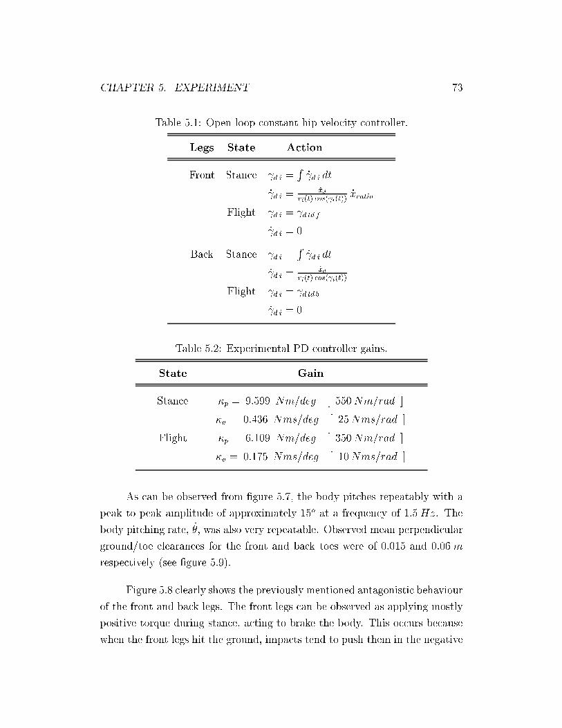
CHAPTER 5. EXPERIMENT 73
Table 5.1: Open loop constant hip velocity controller.
Legs State Action
Front Stance d i =R_ d i dt
_ d i =_xd
ri(t) cos( i(t))_xratio
Flight d i = d td f
_ d i = 0
Back Stance d i =R_ d i dt
_ d i =_xd
ri(t) cos( i(t))
Flight d i = d td b
_ d i = 0
Table 5.2: Experimental PD controller gains.
State Gain
Stance �p = 9:599 Nm=deg [ 550Nm=rad ]
�v = 0:436 Nms=deg [ 25Nms=rad ]
Flight �p = 6:109 Nm=deg [ 350Nm=rad ]
�v = 0:175 Nms=deg [ 10Nms=rad ]
As can be observed from �gure 5.7, the body pitches repeatably with a
peak to peak amplitude of approximately 15o at a frequency of 1:5Hz. The
body pitching rate, _�, was also very repeatable. Observed mean perpendicular
ground/toe clearances for the front and back toes were of 0:015 and 0:06 m
respectively (see �gure 5.9).
Figure 5.8 clearly shows the previously mentioned antagonistic behaviour
of the front and back legs. The front legs can be observed as applying mostly
positive torque during stance, acting to brake the body. This occurs because
when the front legs hit the ground, impacts tend to push them in the negative

CHAPTER 5. EXPERIMENT 74
Table 5.3: Open loop constant hip velocity controller parameters.
Parameter Value
d td f 0o [ 0 rad: ]
d td b 26o [ 0:453 rad: ]
_xd 0:2m=s
_xratio 15 %
direction, thus increasing position tracking errors. To compensate for this
error, a positive hip torque is applied by the robot, resulting in a clockwise
couple on the body, helping to lift the back legs o� the ground. Conversely,
the back legs apply a negative torque during stance helping to propel the body
forward. Considerable tracking error also develops in the back legs in part due
to the large impacts during state transitions from ight to stance (see �gure
5.8). A formal discussion tracking error sources is presented in section 5.3.2.
In terms of forward velocity tracking, although we are commanding the
back legs to track _xd = 0:2m=s, the mean forward velocity of the COM closer
to 0:128 m=s1, revealing a mean velocity tracking error of approximately
35%. A close look at the forward velocity pro�le of the body reveals peak
velocity values alternating between 0:5 and �0:2m=s. This large deviation is
consistent with forward speed variations for the compliant walking algorithm
described in section 4.4.
A close look at the commanded and actual front leg trajectories (see
�gure 5.8), helps to explain some of these variations. Although the front legs
are commanded to sweep in stance, they only move about 2:5o, with half of
the de ection resulting from poor tracking. These errors are a consequence
of the signi�cant impacts experienced by the front legs at touchdown and
from belt backlash in Scout's actuation system. Given this minor front leg
displacement, the front legs can be thought of as remaining �xed throughout
1calculated o� line from data shown in �gure 5.7.

CHAPTER 5. EXPERIMENT 75
Figure 5.6: Key frames of Scout II in a bounding walk. Four distinct phases
are observable : 1) Single Support (Back), 2) Double Support (Back to Front),
3) Single Support (Front), and 4) Double Support (Front to Back)
the stride. This is consistent with previous �ndings by Yamazaki [64] who
obtained stable open loop sti� legged walking, by commanding the front leg
to remain perpendicular to the body (refer to section 2.4.3 for more details).
The sharp decelerations in forward velocity resulting from maintaining the
front legs �xed, contribute to lifting the robot's hind legs o� the ground, at
the expense of producing large variations in forward speed.
Figure 5.9 also provides insight into some important, yet previously un-
modeled system dynamics. As can be seen from this �gure the back leg de ec-
tion does not match the parabolic pro�le expected for a spring mass system
sliding in a frictionless slot. The plotted data clearly shows that the back leg
length actually remains constant for signi�cant portions of the stance period.
This further emphasises the presence of signi�cant Coulomb friction in Scout
II's current leg design (as mentioned in section 5.2).
Since Coulomb friction is proportional to the normal leg contact force,
it makes sense that its e�ects would be more pronounced on the back rather

CHAPTER 5. EXPERIMENT 76
170 171 172 173 174 175 176 177 178 179 180
−10
−5
0
5
10
170 171 172 173 174 175 176 177 178 179 180−150
−100
−50
0
50
100
150
170 171 172 173 174 175 176 177 178 179 180−1
−0.5
0
0.5
1
170 171 172 173 174 175 176 177 178 179 180−1
−0.5
0
0.5
1
t (s)
�(deg)
_ �(deg=s)
_x(m=s)
_y(m=s)
Figure 5.7: Robot torso behaviour during constant hip velocity walk with
parameters from table 5.3. Presented velocity estimates are calculated online
Scout using kinematics.
than the front legs. Not only do the back legs apply larger torques for more
signi�cant periods of time (i.e. the back stance period is much larger than
that of the front leg) than the front legs, but the back legs must also actively
support all of the robot's weight, while trying to propel the robot forward.
Despite these controller characteristics, the proposed dynamic compliant
walking algorithm proved quite stable converging quickly to steady state walk-
ing. Variations in terrain slope and ground friction, had minor yet observable
e�ects on controller performance.

CHAPTER 5. EXPERIMENT 77
170 171 172 173 174 175 176 177 178 179 180−3
−2
−1
0
1
γ 1 (de
g.)
170 171 172 173 174 175 176 177 178 179 180−40
−20
0
20
40
τ 1 (N
m)
170 171 172 173 174 175 176 177 178 179 18010
15
20
25
30
35
γ 2 (de
g.)
170 171 172 173 174 175 176 177 178 179 180−40
−20
0
20
40
τ 1 (N
m)
t (s)
Figure 5.8: Front and back desired (dashed) and actual (solid) leg trajectories
and torques for walk with parameters from table 5.3.
5.3.2 Actuator Limits
Although stable and repeatable walking was obtained for Scout, one issue
which remains to be addressed in our discussion of experimental results, is
the discrepancy between commanded and applied motor torques observed in
�gure 5.8. Similar errors can also be seen in the front legs, however they are
much less severe. Understanding the source of these errors can potentially help
improve trajectory tracking in our walking algorithm or in uence the design
of future walking algorithms.

CHAPTER 5. EXPERIMENT 78
170 171 172 173 174 175 176 177 178 179 1800.26
0.28
0.3
0.32
Leg 1 (
m)
170 171 172 173 174 175 176 177 178 179 1800.26
0.28
0.3
0.32
Leg 2 (
m)
170 171 172 173 174 175 176 177 178 179 180
0
0.02
0.04
0.06
0.08
Toe
1 (m
)
170 171 172 173 174 175 176 177 178 179 180
0
0.02
0.04
0.06
0.08
Toe
2 (m
)
t (s)
Figure 5.9: Front and back leg lengths and perpendicular ground/toe clear-
ances for walk with parameters from table 5.3.
Given Scout's requirements for autonomous operation, we must use light
weight motors to extend operating life. Unfortunately, as touched upon in
sections 1.3 and 4.3.2, this has the undesirable side e�ect of forcing actuators
to be used in peak power regions, where the maximum achievable torque is
highly dependent on motor velocity.
Currently, Scout uses fourMaxon 118777 brushed 90 W DC motors, each
controlled by a Advanced Motion Controls 12A8E PWM servo ampli�er [16].
These motors operate at 24 V, a limit set by the robot's batteries, and are
current limited to 12 A, a constraint imposed by the motor ampli�ers.

CHAPTER 5. EXPERIMENT 79
Given these operating conditions, the torque/speed characteristics pre-
viously shown in �gure 4.5 determine the allowable motor torque that may
be delivered by the motor at a particular shaft speed. Figure 5.10 shows the
applied torques versus angular speed for legs one and two during] a typical
walking experiment. As can be observed, the applied torques remain inside
the torque/speed polygon speci�ed by the motor model. It is interesting to
note, however, that there is still a discrepancy between the theoretical torque
limit and the torque applied in experiment (as shown in �gure 5.10), since
applied torque does not reach the polygonal torque limits.
−20 0 20
−100
−50
0
50
100
ω (
rpm
)
τ1 (Nm)
−20 0 20
−100
−50
0
50
100ω
(rp
m)
τ2 (Nm)
Figure 5.10: Applied front and back leg torque vs. speed : Experiment. The
motor's torque/speed limits restrict applied torques at a particular velocity to
remain inside the indicated parallelogram.
Using the simple DC motor model of �gure 5.11, and applying Kircho�'s
voltage law, the motor terminal voltage VT can be shown to be,
VT = iARA + EA + LA
diA
dt(5.2)
where RA is the armature resistance, EA is the motor back EMF, LA

CHAPTER 5. EXPERIMENT 80
Figure 5.11: DC Motor and Battery Model
is the motor inductance, and iA is the motor current. Assuming quasi-static
motor operation (i.e. diAdt� 0) and using the fact that,
EA = K! ! (5.3)
� = KT iA (5.4)
it can be shown that the maximum achievable motor torque � that can
be produced at a particular velocity ! is,
� =KT
RA
(VT �K! !) : (5.5)
In equation 5.5, KT is the motor torque constant and K! is the motor
speed constant. Key motor parameters are summarised in table 5.4.
Furthermore, using a simple battery model, the terminal voltage VT can
be further expressed as,

CHAPTER 5. EXPERIMENT 81
Table 5.4: Parameters used for voltage compensated torque/speed limit.
Parameter Value
KT 0:0389 Nm=A
K! 0:00406 V=rpm
RA 1:23
Ngearhead 72:38 : 1
�belt 0:8
VT = Vbat � Rbat iA
= Vbat � Rbat �
KT
(5.6)
thus reducing equation 5.5 to,
� =KT
RA�(Vbat �K! !) (5.7)
where � =�1 + Rbat
RA
�.
Figure 5.12 helps better understand the signi�cance of equation 5.7.
Speci�cally, �gure 5.12b shows the large di�erences that exist between com-
manded (dash-dot line) and applied motor torques (solid line) during a typical
period of back leg stance.
Recall that so far our discussion of the motor torque/speed limit has
assumed 24 V operation. Plotting equation 5.5 with VT = 24V on �gure 5.12b
(dotted line) shows that the nominal motor voltage accounts for a large portion
of the errors. As shown in �gure 5.12a, however, the motor terminal voltage
drops far below 24 V during normal operation (a result of the battery's internal
resistance). Recalculating, the maximum achievable torque as per equation

CHAPTER 5. EXPERIMENT 82
171.2 171.3 171.4 171.517.5
20
22.5
25
t (s)
Vol
tage
(V
)a)
171.2 171.3 171.4 171.5
−35
−30
−25
−20
−15
−10
−5
0
5b)
t (s)T
orqu
e (N
m)
Desired Torque Actual Torque 24 V Torque Limit Voltage Compensated Limit
Figure 5.12: a) Supply voltage during a walking stride. b) Actual (solid),
desired (dash-dot), 24 V limit, and voltage compensated torques for a walking
stride : Experiment
5.7 given the terminal voltage, accounts for remaining errors in torque and
provide an excellent match to experimentally applied torque (dashed line).
Figure 5.13, shows that using the measured battery current and an in-
ternal battery resistance Rbat = 0:25 , we can get a good match between
measured motor terminal voltage (solid line) and estimated terminal voltage
(dotted line).
5.3.3 Open Loop Controller Stability
To test controller stability an experiment was conducted in which the robot
walking procedure was started under three di�erent conditions. Firstly, a
robot walk was started using a normal startup procedure. This was done by
leaning the robot onto its front legs and giving the body a small negative pitch.
Secondly, the robot was started from a large negative angle of approximately
�30o. Lastly, the walk was started by placing the robot on its back legs

CHAPTER 5. EXPERIMENT 83
170.8 170.9 171 171.1 171.2 171.3 171.4 171.516
17
18
19
20
21
22
23
24
25
26
t (s)
Vol
tage
(V
)
Figure 5.13: Motor terminal voltage (solid) and calculated battery voltage
based on internal battery resistance (dotted line) using internal battery voltage
Vbat = 25V , Rbat = 0:25, and current drawn during operation iA: Experiment
and giving the body a large positive angle of approximately 30o. As can be
observed from �gure 5.14, for all three vastly di�erent startup conditions, the
maximum body pitch of the robot, �max, converged back to the nominal pitch
walking value within three strides. Stable walking was observed in all three
cases.
These results are encouraging and validate the stability of the open loop
walking controller. However they are also not entirely surprising given our
previous observations of lossy dynamics mentioned in section 5.3.1. Since the
passive unforced system response is almost completely attenuated by the high
system losses, convergence is almost entirely dependent on the energy added
to the system by the controller. Therefore, although the controller was stable,
this came at the expense of a walking gait requiring substantial power.

CHAPTER 5. EXPERIMENT 84
2 4 6 8 10 12 14 16 18 200
2
4
6
8
10
12
14
16
18
20θ m
ax (
deg.
)
Stride
Normal Walk Walk From Large Negative AngleWalk From Large Positive Angle
Figure 5.14: Open loop controller stability test results. The walking controller
is started from three di�erent conditions : 1) Normal startup condition 2)
Startup from large negative angle 3) Startup from large positive angle.
5.4 Walking Energetics
One of the strong motivations for the study of underactuated legged robots is
that reducing actuated degrees of freedom and exploiting passive dynamical
system behaviour can lead to substantial energy savings. However, to be able
to objectively compare energy consumption of various systems (both legged
and wheeled) a fair measure must be used that takes vehicle weight, size,
speed, and con�guration into account. In 1950, Gabrielli and von K�arm�an [22]
proposed a measure of locomotion energetics called specific resistance ( " ),
" =P
mg vmax
: (5.8)

CHAPTER 5. EXPERIMENT 85
Speci�c resistance is de�ned as the ratio of output power P , to the
product of maximum speed vmax, and vehicle weight mg. This expression can
be further generalised to,
"(v) =P (v)
mg v(5.9)
to measure " at various locomotion speeds. By plotting " against speed,
Gabrielli and von K�arm�an compared the energetic performance of land, air,
and sea vehicles, as well as of biological systems of the same scale.
More recently Gregorio and Buehler [28] presented a comparative study
of the speci�c resistance of animals, as well as wheeled and legged vehi-
cles/robots. Their study, found large variations in the literature with respect
to how output power was measured for each vehicle. Cars tended to quote
power at maximum acceleration, rather than maximum speed. Other vehicles,
which reported low speci�c resistances, made use of short term power storage
devices, such as ywheels, reducing power consumption. Published results also
neglected to take into account that in contrast to many conventional wheeled
vehicles, which carry their power sources, few legged robots currently do so.
In addition to the above inconsistencies, the issue of which type of power
to consider is also not clear. To date, most robotics researchers have used use
mechanical power when evaluating system power consumption [28, 51]. Al-
though this provides useful insight into system energetics, yielding a platform
independent measure of eÆciency it does not tell the whole story. Given the
increasing amount of electronic hardware on robots and the fact that me-
chanical power does not account for the signi�cant energy losses due to heat
dissipation, which can be quite signi�cant for conventional electric actuators,
a more realistic measure of system energetics should be based on electrical
power.
Thanks to some custom hardware recently integrated onto Scout II, we
have been able to measure electrical voltage and current levels throughout

CHAPTER 5. EXPERIMENT 86
experiments. In the near future, this capability will allow online battery ca-
pacity estimation letting Scout know how much useful operating life remains
before it needs to \ask" for a recharge. This may also allow the robot to
automatically transition between di�erent gaits in order to operate optimally
at various travel speeds. Figure 5.15 shows the obtained measurements for
battery voltage and current for the same ten second walk shown in �gures
5.7 - 5.9. As touched upon in section 5.3.2, both battery voltage and current
deviate signi�cantly from steady state values during normal operation of the
robot. Voltage can be seen to reach peak values between 17 - 24.5 V. Current
also oscillates repeatedly between 2 - 25 A. Figure 5.16 shows the calculated
electrical and mechanical power from the robot. Electrical and mechanical
power are calculated via,
Pelectrical = V I (5.10)
Pmechanical =
4Xi=1
j �i _�i j (5.11)
respectively. As anticipated the di�erence between input electrical power
and output mechanical power is signi�cant. For a mean input power of 234
W output mechanical power is 24 W, about one tenth the input power.
To obtain an estimate of speci�c resistance for Scout II, data from 10
walking experiments was gathered. Given the narrow range of operation
speeds for the open loop controller, speci�c resistance could only be found
for velocities ranging from 0:09 � 0:15 m=s. Average velocity, as well as
electrical and mechanical power consumption for each of these experiments
was calculated. Once plotted a second order least square regression was �t to
the obtained data.
The results from this analysis are very encouraging. Plotted estimates
of " using mechanical power in �gure 5.17 yield speci�c resistance values as
low as those for Monopod II (0.7) [1, 2], one of the most eÆcient robots to

CHAPTER 5. EXPERIMENT 87
170 171 172 173 174 175 176 177 178 179 180
16
18
20
22
24
26
Vol
tage
(V
)
Supply Voltage
170 171 172 173 174 175 176 177 178 179 1800
5
10
15
20
25
30
t (s)
Am
ps (
A)
Supply Current
Figure 5.15: Battery voltage and current measurements obtained from the
robot for a typical 10 second walk. Controller settings for this walk are listed
in table 5.3.
date, even though we know from previous discussion that few passive dynam-
ical e�ects are currently being used by Scout in walking. Although it still
remains to be experimentally con�rmed, it is believe that even lower speci�c
resistance values could be obtained for running gaits, since the robot will be
travelling substantially faster, with similar power requirements. A perhaps
less encouraging realisation is the need to improve Scout's electrical eÆciency,
since the low 10% eÆciency leaves much to desire. This issue will need to be
addressed if the robot is ever to be used in real life applications, that require
substantial periods of operation between recharges.

CHAPTER 5. EXPERIMENT 88
170 171 172 173 174 175 176 177 178 179 1800
100
200
300
400
500
Pow
er (
W)
Electrical Power (mean =233 W)
170 171 172 173 174 175 176 177 178 179 1800
100
200
300
400
500
t (s)
Pow
er (
W)
Mechanical Power (mean =24 W)
Figure 5.16: Electrical and mechanical power for 10 second open loop walk
whos controller settings are listed in table 5.3. 28 W steady state electrical
power indicated by dashed line in top plot.
0.05 0.1 0.15 0.20.5
0.55
0.6
0.65
0.7
0.75
0.8
0.85
0.9
0.95
1ε (Mechanical)
ε
velocity (m/s)0.05 0.1 0.15 0.24
5
6
7
8
9
10
11
12
13
ε (Electrical)
velocity (m/s)
Figure 5.17: Mechanical and electrical speci�c resistance for a set of 10 exper-
imental runs.

CHAPTER 5. EXPERIMENT 89
5.5 Summary
This chapter presented �ndings from walking experiments on Scout. Although
rocking was not realized, a new walking algorithm based on commanding
constant hip velocity was proposed. This algorithm was stable within a small
region of operating conditions. An analysis of gathered data helped to pin
point previously unmodeled dynamical e�ect helping to explain discrepancies
between experiment and simulation. In addition, electrical and mechanical
speci�c resistances were measured. Speci�c resistance measurements for Scout
II, based on mechanical power, matched those of Monopod II, one of the most
eÆcient robots to date. This suggests that if Scout's design can be re�ned, it
may become a truly useful legged robotic platform for research and real world
applications.

Chapter 6
Conclusion
This thesis presented research on the successful development of a dynamic
compliant walking algorithm for the Scout II robot. This was achieved using
a simple open loop control strategy that commanded constant hip velocity dur-
ing periods of leg stance and two decoupled leg state machines to synchronise
leg actions.
The success of this simple controller parallels previous �ndings at McGill's
Ambulatory Robotics Lab (ARL), showing that seemingly complex behaviours
can be achieved using simple control strategies. Understanding the limits of
this approach is the �rst step in producing truly useful and versatile robots.
The help gain a better understanding of dominant dynamical factors
in uencing robot locomotion, an iterative approach of simulation, analysis,
and experimentation was used. This approach has motivated the following
conclusions:
� Mechanical complexity is not a requisite for obtaining complex loco-
motory behaviour from a walking robot. This said, it is unlikely that
a single robot will accommodate all gaits with the same energetic eÆ-
ciency. In particular, a design such as Scout's that does not use knees,
is better suited for running rather than walking gaits. This is supported
90

CHAPTER 6. CONCLUSION 91
by the fact that running gaits can use ballistic phases of motion to store
greater amounts of energy in leg springs. Vertical energy can thus be
re-introduced into locomotion, without the need for the large touchdown
angles used in walking. Furthermore, given the touchdown impacts seen
in running, larger toe/ground normal forces also develop, helping to re-
duce the occurrence of slip during stance.
� Scout's walking gait could be much improved with the redesign of the
robot's legs. In particular reducing sliding friction would help make
both walking and running more eÆcient. This would also allow locomo-
tion controllers to take full advantage of the system's unforced response,
helping to simplify control algorithms. Strategies such as the natural
frequency rocking and walking controllers developed in chapter 4 could
then be used. In the area of running, reducing sliding friction would most
likely increase maximum achievable speeds and pitching amplitude, two
desirable qualities for rough terrain locomotion. Until the robot's leg
design is modi�ed, future simulations should incorporate sliding friction
e�ects in prismatic leg models. Leg de ection tests such as those de-
scribed in section 5.2 could be used to yield estimates of Coulomb leg
friction.
� Having found the signi�cant e�ect variations in supply voltage can have
on motor torque/speed limitations and on the controller e�ectiveness,
future work should use more conservative estimates of achievable torque,
both in simulation and experiment. Doing this should not only help
to bring simulation and experimental results in tighter correspondence
with one another. Robot design alternatives also exist to help improve
these characteristics. A reevaluation of the power supply system on
Scout may warrant increasing the robot's operation voltage to expand
the polygon of torques that may be applied for a given leg speed. A
safer approach might be to �nd a way of reducing voltage variations
in the system. Having said this, these hardware modi�cations would
not magically solve the torque/speed constraints Scout currently faces,
since increasing torque during leg slip, would aggravate the problem

CHAPTER 6. CONCLUSION 92
rather than help to solve it.
As is the case with most research, results always produce more new
questions than answers. Interesting avenues for future research include:
� Attempts to further simplify the developed walking controller. If a ver-
sion of the proposed constant hip velocity controller can be implemented
using only proprioceptive sensing, that is, controlling the relative angle
between legs and body, instead of the leg angle with respect to vertical,
this may allow for the design of an even simpler legged robot platform,
through the elimination of redundant sensing.
� A comparative study of walking versus running energetics on Scout
II. This would be an interesting way of learning more about system
behaviour and formally identifying eÆcient locomotion modes for the
robot.
� A study of gait transitions between walking and running. As mentioned
power sensing hardware may allow transitions to occur autonomously
once running energetics is better understood.
� Use of linear or rotary knee actuation. Given that walking and running
are known to be achievable with Scout's current mechanical con�gu-
ration, using only one actuated degree of freedom per leg, these extra
actuators could help to provide additional control \knobs", helping to
further re�ne current locomotion gaits.

Bibliography
[1] M. Ahmadi and M. Buehler. A control strategy for stable passive running.
Proc. IEEE/RSJ Int. Conf. Intelligent Systems and Robots, pages 152{
157, August 1995.
[2] M. Ahmadi and M. Buehler. The arl monopod ii running robot: Control
and energetics. Proc. IEEE Int. Conf. Robotics and Automation, pages
1689{1694, May 1999.
[3] R. McN. Alexander. Elastic Mechanims in Animal Movement. Cambridge
University Press, Cambridge, 1988.
[4] J. Bares, M. Hebert, T. Kanade, E. Krotkov, T. Mitchelland R. Sim-
mons, and W. Whittaker. Ambler: An autonomous rover for planetary
exploration. IEEE Computer, 22(6):18{26, June 1989.
[5] J. Bares and David S. Wettergreen. Dante ii : Technical description,
results, and lessons learned. Int. J. Robotics Research, 18(7):621{649,
July 1999.
[6] R. Battaglia. Design of the scout ii quadruped with preliminary stair-
climbing. Master thesis, McGill University, Montr�eal, Quebec, Canada,
March 1999.
[7] F. P. Beer and E. R. Johnston Jr. Vector Mechanics for Engineers DY-
NAMICS. McGraw Hill Book Co., Toronto, 1988.
93

BIBLIOGRAPHY 94
[8] M. D. Berkemeier. Approximate return maps for quadrupedal running.
In Proc. IEEE Int. Conf. Robotics and Automation, volume 1, pages 805{
810, Albuquerque, NM, April 1997.
[9] R. A. Brooks. A robust layered control system for a mobile robot. Tech-
nical report, MIT AI Memo 864, September 1985.
[10] M. Buehler, R. Battaglia, A. Cocosco, G. Hawker, J. Sarkis, and K. Ya-
mazaki. Scout: A simple quadruped that walks, climbs, and runs. Proc.
IEEE Int. Conf. Robotics and Automation, pages 1701{1712, 1998.
[11] M. Buehler, A. Cocosco, K. Yamazaki, and R. Battaglia. Stable open
loop walking in quadruped robots with sti� legs. Proc. IEEE Int. Conf.
Robotics and Automation, pages 2348{2353, May 1999.
[12] C. M. Chew, J. E. Pratt, and G. A. Pratt. Blind walking of a planar
bipedal robot on sloped terrain. In Proc. IEEE Int. Conf. Robotics and
Automation, Detroit, MI, 1999.
[13] A. Cocosco. Control of walking in a quadruped robot with sti� legs.
Master thesis, McGill University, Montr�eal, Quebec, Canada, July 1998.
[14] J. J. Collins and I.N. Stewart. Coupled nonlinear oscillators and the
symmetries of animal gaits. Journal of Nonlinear Science, 73:349{392,
1993.
[15] PC104 Consortium. PC/104 Embedded-PC Modules.
http://www.pc104.org.
[16] Advanced Motion Controls. PWM Servo Ampli�ers Catalogue.
http://www.a-m-c.com/, 1992.
[17] SONY Corporation. SONY World Homepage.
http://www.world.sony.com/, 2000.
[18] A. Daberkow, J. Gao, and W. Schielden. Walking without impacts.
CISM-IFToMM Symposium on the Theory and Practice of Robots and
Manipulators, pages 340{348, 1990.

BIBLIOGRAPHY 95
[19] E. R. Dunn and R. D. Howe. Towards mooth bipedal walking. In Proc.
IEEE Int. Conf. Robotics and Automation, pages 2489{2494, 1994.
[20] E. R. Dunn and R. D. Howe. Foot placement and velocity control in
smooth bipedal walking. In Proc. IEEE Int. Conf. Robotics and Automa-
tion, pages 578{583, Minneapolis, MN, Apr 1996.
[21] M. H. Raibert et al. Dynamically stable legged locomotion. Technical
Report CMU-LL-4-1985, Carnegie-Mellon University, 1985.
[22] G. Gabrielli and T. H. von Karman. What price speed ? Mechanical
Engineering, 72(10):775{781, 1950.
[23] P. Gambayran. How Mammals Run : Anatomical Adaptations. John
Wiley and Sons, Inc., New York, 1974.
[24] M. Garcia, A. Chatterjee, and A. Ruina. Speed, eÆciency, and stability
of small-slope 2-d passive dynamic biped walking. In Proc. IEEE Int.
Conf. Robotics and Automation, Leuven, Belgium, May 1998.
[25] A. Goswami. Foot rotation indicator (fri) point: A new gait planning
tool to evaluate postural stability of biped robots. In Proc. IEEE Int.
Conf. Robotics and Automation, pages 47{52, Detroit, MI, May 1999.
[26] A. Goswami. Postural stability of biped robots and the foot rotation
indicator (fri) point. Int. J. Robotics Research, 18(6), 1999.
[27] P. Gregorio. Design, control and energy minimization strategies for an
electrically actuated legged robot. Master's thesis, McGill University,
Montr�eal, Quebec, Canada, August 1994.
[28] P. Gregorio, M. Ahmadi, and M. Buehler. Design, control, and energetics
of an electrically actuated legged robot. IEEE Trans. Systems, Man, and
Cybernetics, 27B(4):626{634, August 1997.
[29] S. Grillner. Neurobiological bases of rhythmic motor acts in vertebrates.
Science, 228:143{149, 1985.

BIBLIOGRAPHY 96
[30] K. Sakurama H. Kimura and S. Akiyama. Dynamic walking and running
of the quadruped using neural oscillator. In Proc. IEEE/RSJ Int. Conf.
Intelligent Systems and Robots, pages 50{57, Victoria, October 1998.
[31] G. Hawker and M. Buehler. Quadruped trotting with passive knees -
design, control, and experiments. Proc. IEEE Int. Conf. Robotics and
Automation, April 2000.
[32] K. Hirai, M. Hirose, Y. Haikawa, and T. Takenaka. The development of
Honda humanoid robot. In Proc. IEEE Int. Conf. Robotics and Automa-
tion, pages 1321{1326, Leuven, Belgium, 1998.
[33] D. F. Hoyt and C. R. Taylor. Gait and the energetics of locomotion in
horses. Nature, 292:239{240, 1981.
[34] Associated Spring Raymond. Barnes Group Inc. SPEC : Stock Springs,
Spring Washers and Retaining Rings. http://www.barnesgroupinc.com/,
1995.
[35] G. A. Pratt J. E. Pratt, P. Dilworth. Virtual model control of a bipedal
walking robot. In Proc. IEEE Int. Conf. Robotics and Automation, pages
193{198, Albuquerque, NM, April 1997.
[36] H. Kimura. Realization of dynamic walking and running of the quadruped
using neural oscillator. In 5th Int. Conf. on Simulation of Adaptive Be-
havior (SAB98), Workshop on Biological Inspired Walking, pages 7{15,
Zurich, 1998.
[37] H. Kitano, M. Fujita, S. Zrehen, and K. Kageyama. Sony legged robot
for robocup challenge. volume 3, pages 2605{2612, 1998.
[38] QNX Software Systems Ltd. QNX TCP/IP Users Guide. 1994.
[39] K. Matsuoka. Sustained oscillations generated by mutually inhibiting
neurons with adaptation. Biological Cybernetics, 52:367{376, 1985.
[40] T. McGeer. Passive dynamic walking. Int. J. Robotics Research, 9(2):62{
82, 1990.

BIBLIOGRAPHY 97
[41] T. McGeer. Passive walking with knees. In Proc. IEEE Int. Conf. Robotics
and Automation, pages 1640{1645, Cincinnati, OH, May 1990.
[42] R. McGhee and K. Waldron. The adaptive suspension vehicle project: A
case study in the development of an advanced concept for land locomo-
tion. In Unmanned Systems, pages 34{43, Summer 1985.
[43] R. B. McGhee and A. A. Frank. On the stability properties of quadruped
creeping gaits. Mathematical Biosciences, 3:331{351, 1968.
[44] D. A. Messuri and C. A. Klein. Automatic body regulation for main-
taining stability of a legged vehicle during rough terrrain locomotion. In
Proc. IEEE Int. Conf. Robotics and Automation, pages 132{141, 1985.
[45] E. Muybridge. Animals in Motion. Dover Publications, Inc., New York,
1957.
[46] P. V. Nagy, S. Desa, and W. L. Whittaker. Energy-based stability mea-
sures for reliable locomotion of statically stable walkers : Theory and
application. Int. J. Robotics Research, RA-1(3):272{287, 1994.
[47] A. Neishtadt and Z. Li. Stability proof of raibert's four-legged hopper
in bounding gait. Technical Report 578, New York University, Courant
Institute, New York, N.Y., Sep 1991.
[48] D. Papadopoulos. Stable running for a quadruped robot with compli-
ant legs. Master's thesis, McGill University, Montr�eal, Quebec, Canada,
February 2000.
[49] D. Papadopoulos and M. Buehler. Stable running in a quadruped robot
with compliant legs. Proc. IEEE Int. Conf. Robotics and Automation,
April 2000.
[50] J. E. Pratt. Virtual model control of a biped walking robot. Master
thesis, Massachusetts Institute of Technology, August 1995.
[51] J. E. Pratt and G. A. Pratt. Exploiting natural dynamics in the con-
trol of a planr biped walking robot. In Proceedings of the Thity-Sixth

BIBLIOGRAPHY 98
Annual Allerton Conference on Communicatio, Control and Computing,
Monticello, IL, 1998.
[52] J. E. Pratt and G. A. Pratt. Intuitive control of a planar bipedal walk-
ing robot. In Proc. IEEE Int. Conf. Robotics and Automation, Leuven,
Belgium, 1998.
[53] J. E. Pratt, A. Torres, P. Dilworth, and G. A. Pratt. Virtual actuator
control. In Proc. IEEE/RSJ Int. Conf. Intelligent Systems and Robots,
Osaka, Japan, 1996.
[54] M. H. Raibert. Legged Robots That Balance. MIT Press, 1986.
[55] M. H. Raibert. Trotting, pacing, and bounding by a quadruped robot. J.
of Biomechanics, 1991.
[56] Knowledge Revolution. Working Model 2D User's Guide. San Mateo,
California, 1996.
[57] R. Ringrose. Self-stabilizing running. In Proc. IEEE Int. Conf. Robotics
and Automation, Albuquerque, NM, May 1997.
[58] M. L. Shik, F. V. Severin, and G. N. Orlovsky. Control of walking and
running by means of electrical stimulation to the mid-brain. Biophysics,
11:756{765, 1966.
[59] I. E. Sutherland and M. K. Ullner. Footprints in the asphalt. Int. J.
Robotics Research, 3(2):29{36, 1984.
[60] G. Taga. A model of the neuro-musculo-skeletal system for human lo-
comotion ii - real-time adaptability under various constraints. Biological
Cybernetics, 73:113{121, 1995.
[61] G. Taga, Y. Yamaguchi, and H. Shimizu. Self-organized control of bipedal
locomotion by neural oscillators in unpredictable environment. Biological
Cybernetics, 65:147{159, 1991.
[62] W. Thompson. Theory of Vibration with Applications, Fourth Edition.
Prentice Hall, Englewood Cli�s, New Jersey, 1993.

BIBLIOGRAPHY 99
[63] M. Vukobratovi�c and D. Juricic. Contributions to the synthesis of biped
gait. IEEE Trans. Biom. Eng., BME-16:1{6, 1969.
[64] K.S. Yamazaki. The design and control of scout i, a simple quadruped
robot. Master thesis, McGill University, Montr�eal, Quebec, Canada,
February 1999.

Appendix A
MPC550 Interface Schematics
100

APPENDIX A. MPC550 INTERFACE SCHEMATICS 1011
23
45
67
8
ABCDEFGH
Laser1
Laser2
M1_out
M3_out
M2_out
M4_out
M1_in
M2_in
M3_in
M4_in
B_V
olt
Watchdog
12G
yro1
12G
yro212
AU
X2
12
34
56
7
1413
1211
109
8
DA
C_IP
+12V
123P
1
123P
2
123P
3
123P
4
GN
D
135791113151719
2468101214161820
AD
C_IP
+12V
+5V-12V
R1
3KGN
D
LED
1 +5V
R2
3KGN
D
LED
2 +12V
1234
PO
WE
R
B_C
urr
AU
X1
C10
0.1uF
C7
0.1uF
C5
0.1uF
C8
100 uFC
9100 uF
C6
100 uF
C2
0.1uF
C4
0.1uF
C1
0.1uF
C3
0.1uF
GN
D
GN
D
GN
D
12345 MO
UT3
12345 MO
UT4
12345
MO
UT1
12345
MO
UT2
Pot1
Pot2
Pot3
Pot4
Pot1
Pot2
Pot3
Pot4
GN
D
GN
D
&P
roj:digital.sch&
Proj:scaling.sch
6O
UT
2V
IN
4G
ND
5TR
IM
U4
LT1021N
Sheet
ofM
odified :
Size:
Docum
ent Num
ber:R
ev.:
Sheet T
itle:
File N
ame :
Created :
Am
bulatory Robotics Lab
Cen
tre for In
telligen
t Mach
ines
McG
ill Univ
ersity
MP
C5
50
Inte
rface B
oard
Sch
em
atic
s
20
00
-04
-01
2000-0
7-1
0
analo
g.sch
A
11
.2
31
Montreal, Q
C, C
anad
a, H3A
2A
7
Figure A.1: MPC550 Interface Schematics - 1/3

APPENDIX A. MPC550 INTERFACE SCHEMATICS 1021
23
45
67
8
ABCDEFGH
Watchdog
1234567891011121314151617181920212223242526
DIO
_IP
GN
D Hall_E
ffect1H
all_Effect2
Hall_E
ffect3H
all_Effect4
HE
1R
4
1.1K +5V
HE
2R
5
1.1K +5V
HE
3R
6
1.1K +5V
HE
4R
7
1.1K +5V
GN
D
Hall_E
ffect1
Hall_E
ffect2
Hall_E
ffect3
Hall_E
ffect4
12345678910
TIME
R_IP
GN
D
12
AU
X1_12V
12
AU
X2_12V
12
AU
X1_5V
12
AU
X2_5V
+12V
R13
220 +5V
Tim
er2
Tim
er0
GN
D
8
2
1
T1AZX
MD
63N03X
C14
0.1uF
C15
0.1uF
C16
0.1uF
C17
0.1uF
GN
D
R12
220 +5V
Tim
er1
GN
D
64
3
T2B
ZXM
D63N
03X
R11
220
Tim
er0
GN
D
8
2
1
T2A
123
Servo1
Tim
er1
Tim
er2
123
Servo2
C12
10uF
C13
0.1uF
120uH
120uH
+5V
GN
D
12
F1
1 2
F2
+5V
+5V
231
U5A
74LS02
Watchdog G
ate
Watchdog G
ate
Sheet
ofM
odified :
Size:
Docum
ent Num
ber:R
ev.:
Sheet T
itle:
File N
ame :
Created :
Am
bulatory Robotics Lab
Cen
tre for In
telligen
t Mach
ines
McG
ill Univ
ersity
MP
C5
50
Inte
rface B
oard
- DIO
, Tim
ers &
Misc
.
20
00
-04
-01
20
00
-07
-10
dig
ital.sc
hA
2
1.2
32
Montreal, Q
C, C
anad
a, H3A
2A
7
Figure A.2: MPC550 Interface Schematics - 2/3

APPENDIX A. MPC550 INTERFACE SCHEMATICS 1031
23
45
67
8
ABCDEFGH
M1_out
M2_out
M3_out
M4_out
M1_in
M2_in
M3_in
Laser1
Laser2M
4_in
U1B
LM324
+5V
-12V
R21
51K
R20
62K
U1C
LM324
+5V
-12V
R23
51K
R22
62K
U2A
LM324
+5V
-12V
R25
51K
R24
62K
C20
0.1uF
C21
0.1uF
GN
D
12
C18
10nF1
2C
2210nF
U1A
LM324
+12V
-12V
R37
51K
R36
62K12
L1
U2C
LM324
+5V
-12V
R39
51K
R38
62K12
L2
GN
D
12
C30
10nF
GN
D
12
C19
10nF
GN
D
U2D
LM324
+5V
-12V
R26
51K
R27
62K
C24
0.1uF
12
C23
10nF
GN
D
C25
0.1uFG
ND
12
C31
10nF
Sheet
ofM
odified :
Size:
Docum
ent Num
ber:R
ev.:
Sheet T
itle:
File N
ame:
Created :
Am
bulatory Robotics Lab
Cen
tre for In
telligen
t Mach
ines
McG
ill Univ
ersity
MP
C550 In
terface Board
Sch
ematics - A
DC
Scalin
g
20
00
-04
-01
20
00
-07
-10
scalin
g.0
01
A
11
.2
33
Montreal, Q
C, C
anad
a, H3A
2A
7
Figure A.3: MPC550 Interface Schematics - 3/3