composing circular arcs with minimal nurbs · composing circular arcs with minimal nurbs 195...

International Mathematical Forum, 4, 2009, no. 5, 193 - 218

Composing Circular Arcs with Minimal NURBS

Rene Grothmann

Katholische Universitat Eichstatt-IngolstadtMathematisch-Geographische Fakultat

85071 Eichstatt, [email protected]

Manfred Sommer

Katholische Universitat Eichstatt-IngolstadtMathematisch-Geographische Fakultat

85071 Eichstatt, [email protected]

Abstract

We study the problem of constructing a NURBS (nonuniform ratio-nal B-spline curve) with a minimal number of knots forming a given setof continuously resp. smoothly connected circular arcs. In the continu-ous case, NURBS defined by a minimal number of conditions can alwaysbe constructed. In the case when the circular arcs are smoothly con-nected, we give a characterization of the existence of minimal NURBS.

Mathematics Subject Classification: 65D07, 65D17

Keywords: Rational B-splines; conic sections

1 Introduction

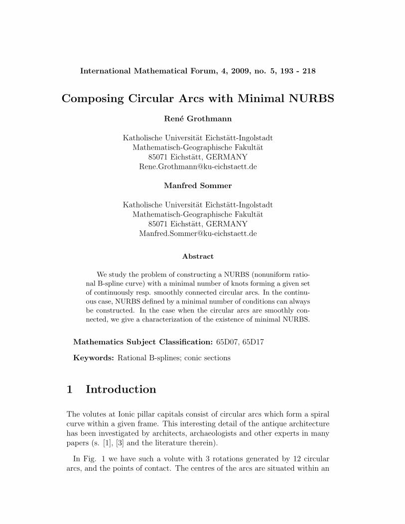
The volutes at Ionic pillar capitals consist of circular arcs which form a spiralcurve within a given frame. This interesting detail of the antique architecturehas been investigated by architects, archaeologists and other experts in manypapers (s. [1], [3] and the literature therein).

In Fig. 1 we have such a volute with 3 rotations generated by 12 circulararcs, and the points of contact. The centres of the arcs are situated within an

194 Rene Grothmann and Manfred Sommer

Figure 1: Volute with 3 rotations and eye

eye on a grid parallel to the axes. They are the vertices of the polygon in Fig.2.

Usually, in the antique architecture a tangential transition has been chosenbetween circular arcs, i.e., both centres of the corresponding arcs and the pointof contact are collinear. But to obtain a regular geometric structure of thepoints of contact certain transitions of the arcs are only ”almost tangential”,and the centres of the corresponding arcs and the point of contact do not lieon a straight line (s. [1], [3]).

Since conic sections can be represented by rational Bezier-curves of degreetwo, it suggests itself to describe connected curves, generated by composedcircular arcs using nonuniform rational B-splines, the so-called NURBS, ofdegree two. In this paper we show how to choose a minimal number of controlpoints and knots in order to construct a NURBS forming continuously resp.smoothly connected circular arcs.

Figure 2: Centres of the arcs from Fig. 1

Since we may assume that the arcs have pairwise different radii or centres,for each arc we need at least one knot interval to represent the arc as a NURBS

Composing Circular Arcs with Minimal NURBS 195

segment. It turns out that the construction of the NURBS is always possible,if we allow double knots. Hence the question arises to give a lower limit for thenecessary number of knots to construct the corresponding NURBS. We firstanswer this question for the case of circular arcs where the changes in adjacentarcs are assumed to be continuous only.

The case of arcs with smooth transitions takes some more effort. We firstgive a lower bound for the number of conditions to construct the correspondingNURBS. In order to show that this number is sufficient, a nonlinear system ofequations has to be solved to determine the weights and knots. Hence we haveto show the existence of a rational spline curve with variable knots. For thecase of two composed circular arcs, we always obtain a solution. Unfortunately,this is no longer true for L > 2 (L denotes the number of arcs). However, weare able to establish a characterization of the existence of solutions for everyL > 2. For some small numbers L, we give the exact formulas for the weightsand knots.

2 The Problem

Assume that L (L ≥ 2) circular arcs K1, . . . , KL are given in R2. Moreover,assume that each Ki belongs to a circle with centre pi and radius ri. Let di−1

and di be the endpoints of Ki, and suppose that

0 < αi < π (2.1)

for the angle αi = ^(di−1,pi,di) at pi, i = 1, . . . , L.

We consider the tangents at Ki in di−1 and di, and denote their intersectionpoint by ci, i = 1, . . . , L. These points exist by (2.1), and satisfy the conditions

‖di−1 − ci‖ = ‖di − ci‖, i = 1, . . . , L, (2.2)

where ‖ · ‖ denotes the Euclidean norm (s. Fig. 3).

Moreover, we assume that

Ki ∪Ki+1 does not form a circular arc for i = 1, . . . , L− 1. (2.3)

Setting

C =L⋃

i=1

Ki

we obtain a connected curve in R2.


Figure 3: Connected circular arcs

We show that C can be represented as a rational B-spline curve of degreetwo. For this, we need an n ∈ N, a knot vector T of the type

T : t0 = t1 = t2 < t3 ≤ . . . ≤ tn < tn+1 = tn+2 = tn+3, (2.4)

control points {bi}ni=0 in R2, and weights {wi}n

i=0 in R such that

C =

r(t) =

n∑i=0

wibiNi(t)

n∑i=0

wiNi(t): t ∈ [t2, tn+1]

, (2.5)

where {Ni}ni=0 denote the normalized B-splines of degree two with knot vector

T (s. [2], [4]).

3 The Continuous Case

Let us assume in this section that there is no tangential transition from Ki toKi+1 in di for i = 1, . . . , L− 1. In order to show that C can be described as aNURBS r by (2.5), we set n = 2L, and choose a fixed knot vector of the type

T : t0 = t1 = t2 < t3 = t4 < . . . < t2L−1 = t2L < t2L+1 = t2L+2 = t2L+3, (3.1)

i.e., t2i−1 = t2i, i = 2, . . . , L, and control points {bi}2Li=0 satisfying

b2i = di, i = 0, . . . , L,b2i−1 = ci, i = 1, . . . , L.

(3.2)


It is well known (s. e.g. [2], [4]) that the B-Splines {Ni}2Li=0 of degree two with

knot vector T can be determined by the following recurrence relation:

N0(t) =

(

t3 − t

t3 − t2

)2

, if t2 ≤ t ≤ t3

0, elsewhere,

N2L(t) =

0, if t2 ≤ t ≤ t2L(

t− t2L

t2L+1 − t2L

)2

, elsewhere,

N2i−1(t) =

2

(t2i+1 − t2i)2(t− t2i)(t2i+1 − t), if t2i ≤ t ≤ t2i+1

0, elsewhere

for i = 1, . . . , L, and

N2i(t) =

(t− t2i

t2i+1 − t2i

)2

, if t2i ≤ t ≤ t2i+1(t2i+3 − t

t2i+3 − t2i+2

)2

, if t2i+2 < t ≤ t2i+3

0, elsewhere

for i = 1, . . . , L− 1. In particular, we obtain for t ∈ [t2j, t2j+1], j = 1, . . . , L:

2L∑i=0

Ni(t) =2j∑

i=2j−2

Ni(t) = 1,

Ni(t) = Bi−2j+2

(t−t2j

t2j+1−t2j

), i = 2j − 2, 2j − 1, 2j,

(3.3)

where {Bi}2i=0 denote the Bernstein-polynomials of degree two. We define the

weights {wi}2Li=0 by

w2i = 1, i = 0, . . . , L,w2i−1 = cos ^(b2i,b2i−2,b2i−1), i = 1, . . . , L.

(3.4)

Following (2.1) we easily verify that

Ki ⊂ ∆(b2i−2,b2i−1,b2i), i = 1, . . . , L, (3.5)

where ∆(·) denotes the triangle with the specified vertices. In view of (2.2), itis easily verified that

0 < w2i−1 =‖b2i − b2i−2‖

2‖b2i−1 − b2i−2‖, i = 1, . . . , L.


Using the above defined parameters, we set

r(t) =

2L∑i=0

wibiNi(t)

2L∑i=0

wiNi(t)

, t ∈ [t2, t2L+1], (3.6)

and prove the following statements.

Theorem 3.1 Assume that r is given as in (3.6). Then the following state-ments hold:

(i) C = {r(t) : t ∈ [t2, t2L+1]};

(ii) If r is a NURBS defined by a knot vector T of the type (2.4), control

points {bi}ni=0 and weights {wi}n

i=0 such that (2.5) holds, i.e.,

C =

r(t) =

n∑i=0

wibiNi(t)

n∑i=0

wiNi(t): t ∈ [t2, tn+1]

.

Then n ≥ 2L.

Proof: (i) Suppose that r is defined by (3.6). We show that

Kj = {r(t) : t ∈ [t2j, t2j+1]}

holds for j = 1, . . . , L. Then, in view of

C =L⋃

j=1

Kj,

the statement follows immediately. Hence let a knot interval [t2j, t2j+1] begiven. Using (3.3), we obtain for t ∈ [t2j, t2j+1]:

r(t) =

2L∑i=0

wibiNi(t)

2L∑i=0

wiNi(t)

=

2j∑i=2j−2

wibiNi(t)

2j∑i=2j−2

wiNi(t)

=

2j∑i=2j−2

wibiBi−2j+2

(t−t2j

t2j+1−t2j

)2j∑

i=2j−2

wiBi−2j+2

(t−t2j

t2j+1−t2j

) .

(3.7)


By (3.4), this implies that r|[t2j ,t2j+1] is a rational Bezier-curve of degree twowith w2j−2 = w2j = 1, and

r(t2j) =w2j−2b2j−2

w2j−2

= b2j−2 = dj−1,

r(t2j+1) =w2jb2j

w2j

= b2j = dj.

In particular, this curve represents a conic section (s. [2]). Since by (3.5)

Kj ⊂ ∆(b2j−2,b2j−1,b2j),

it follows that Kj is described by r|[t2j ,t2j+1] if and only if w2j−1 is defined as in(3.4) [2], i.e., 0 < w2j−1 = cos ^(b2j,b2j−2,b2j−1). Therefore, using this valuefor w2j−1, we obtain:

Kj = {r(t) : t ∈ [t2j, t2j+1]},

j = 1, . . . , L.

(ii) For some n ∈ N let be given a knot vector T of the type (2.4), i.e.,

T : t0 = t1 = t2 < t3 ≤ . . . ≤ tn < tn+1 = tn+2 = tn+3,

control points {bi}ni=0 and weights {wi}n

i=0 such that

C =

r(t) =

n∑i=0

wibiNi(t)

n∑i=0

wiNi(t): t ∈ [t2, tn+1]

.

We show that the relation n ≥ 2L must follow. For the proof we consider arcsKi and Ki+1 for any i ∈ {1, . . . , L − 1}. Since we assume in this section thatthere is no tangential transition between both arcs in di, Ki ∪Ki+1 does notform a continuously differentiable curve. Therefore, it cannot be described bya rational Bezier-curve. This implies that there exist knots tji−1

< tji< tji+1

in T such thatKi = {r(t) : t ∈ [tji−1

, tji]},

Ki+1 = {r(t) : t ∈ [tji, tji+1

]},

hence r(tji) = di. It follows that tji

is a knot of multiplicity at least two.On the contrary, suppose that it is a simple knot, i.e., tji−1 < tji

< tji+1.

Then each B-spline Ni and, therefore, the NURBS r would be continuouslydifferentiable in tji

. But this contradicts the above arguments on Ki ∪ Ki+1.


Hence it follows that tjihas multiplicity at least two for i ∈ {1, . . . , L − 1}.

Thus there exist at least L− 1 double knots in (t2, tn+1) which implies that

n− 2 ≥ 2(L− 1),

and, therefore, n ≥ 2L. This proves statement (ii). 2

Remark 3.2 Theorem 3.1 states that the curve r defined by (3.6) describesthe given curve C by a minimal number of conditions.

4 The Smooth Case

Let us now assume that there is a tangential transition from Ki to Ki+1 in di,i.e., ci,di and ci+1 are collinear for i = 1, . . . , L−1. Of course, we still assumethat the assumptions (2.1) - (2.3) hold.

As in the preceding section we are looking for a minimal NURBS r describingC. As a first result we can apply Theorem 3.1 to the present case, settingn = 2L, and choosing knots, control points and weights as in (3.1), (3.2) and(3.4). Then from statement (i) in Theorem 3.1 we obtain immediately:

Theorem 4.1 Assume that r is defined by (3.6). Then

C = {r(t) : t ∈ [t2, t2L+1]}.

The curve r is defined by 2L + 1 control points. But, as we will show later,for L = 2 the curve C can be described by a NURBS with a smaller numberof control points. Hence in this case r fails to be minimal with respect to thenumber of parameters. Therefore, we are first interested in the question ofhow many parameters are necessary at least to describe C.

Lemma 4.2 If r is a NURBS of type (2.5) which describes C then therelation

n ≥ L + 1

holds.

Proof: Since for each i = 1, . . . , L − 1 the points ci,di, ci+1 are collinear,the L + 2 points {d0, c1, . . . , cL,dL} form a polygon P with the property thatP cannot be represented by a proper subset of these points. Therefore, sinceP can be taken as control polygon of r, and since by the above arguments acontrol polygon with fewer points is impossible, the relation n ≥ L+1 follows.2


In view of Lemma 4.2, we set

n = L + 1,

and define control points {bi}L+1i=0 by

b0 := d0, bi := ci, i = 1, . . . , L, bL+1 := dL.

Moreover, we need weights {wi}L+1i=0 and knots {ti}L+4

i=0 of the type (2.4) suchthat the given curve C is described by a NURBS

r(t) =

L+1∑i=0

wibiNi(t)

L+1∑i=0

wiNi(t)

, t ∈ [t2, tL+2]. (4.1)

Note that such a curve r is minimal according to Lemma 4.2. Since by (2.3)r is not arbitrarily often differentiable in di, i = 1, . . . , L− 1, there must existknots tji−1

< tji< tji+1

such that

Ki = {r(t) : t ∈ [tji−1, tji

]},Ki+1 = {r(t) : t ∈ [tji

, tji+1]}.

This implies r(tji) = di for i = 1, . . . , L− 1. Moreover, since the knots satisfy

the property

t0 = t1 = t2 < t3 ≤ . . . ≤ tL+1 < tL+2 = tL+3 = tL+4,

the relationr(ti+2) = di, i = 1, . . . , L− 1

must hold. Then the property di 6= di+1 for all i implies that

t0 = t1 = t2 < t3 < t4 < . . . < tL+1 < tL+2 = tL+3 = tL+4. (4.2)

Thus, to solve our problem we have to find a knot vector T of the type (4.2)with simple knots {ti}L+1

i=3 and weights {wi}L+1i=0 such that

C = {r(t) : t ∈ [t2, tL+2]}, (4.3)

where r is defined by (4.1). We may set

w0 = 1 and t2 = 0.

Since the B-splines {Ni}L+1i=0 are invariant under a linear transformation of

T , we may fix the knot tL+2. Hence we still have to determine 2L parameters


w1, . . . , wL+1, t3, . . . , tL+1. In order to solve (4.3) these parameters must satisfythe following conditions:

r(ti+2) = di, i = 1, . . . , L− 1,

r(ti) ∈ Ki for some ti ∈ (ti+1, ti+2), i = 1, . . . , L.(4.4)

We will show in Theorem 4.3 that a curve r satisfying (4.4) describes the givencurve C. Moreover, we will show in Remark 4.4 that (4.4) leads to a nonlinearsystem of 2L− 1 equations for the 2L parameters

w1, . . . , wL+1, t3 < t4 < . . . < tL+1.

It turns out that we may also fix the knot t3 such that

0 = t2 < t3 < tL+2.

Theorem 4.3 Assume that a NURBS r is given by (4.1) with knot vectorT by (4.2) which satisfies the conditions (4.4). Then the following statementshold:

(i) Ki = {r(t) : t ∈ [ti+1, ti+2]}, i = 1, . . . , L;

(ii) wi > 0, i = 0, . . . , L + 1;

(iii)

wi+1 = witi+3 − ti+2

ti+2 − ti+1

‖di − bi‖‖di − bi+1‖

=ti+3 − ti+2

ti+2 − ti+1

miwi,

where

mi :=‖di − bi‖‖di − bi+1‖

, i = 1, . . . , L− 1.

Proof: (i) Assume that r is given by (4.1) with knot vector T by (4.2) andlet i ∈ {1, . . . , L}. Since

Nj(t) = 0, t ∈ Ii := [ti+1, ti+2], j 6= i− 1, i, i + 1,

only the B-splines {Nj}i+1j=i−1 are relevant for Ii. These are determined by the

well known recurrence relation (s. [2]) for t ∈ Ii as follows:

Ni−1(t) =(ti+2 − t)2

(ti+2 − ti+1)(ti+2 − ti),

Ni(t) =(t− ti)(ti+2 − t)

(ti+2 − ti+1)(ti+2 − ti)+

(ti+3 − t)(t− ti+1)

(ti+3 − ti+1)(ti+2 − ti+1),

Ni+1(t) =(t− ti+1)

2

(ti+3 − ti+1)(ti+2 − ti+1).


In particular, we obtain for t ∈ Ii:

1 =L+1∑j=0

Nj(t) =i+1∑

j=i−1

Nj(t).

Moreover, the Bernstein-polynomials {Bj}2j=0 related to Ii can be rewritten as

B0(t) =ti+2 − ti

ti+2 − ti+1

Ni−1(t),

B1(t) = Ni(t)−ti+1 − ti

ti+2 − ti+1

Ni−1(t)−ti+3 − ti+2

ti+2 − ti+1

Ni+1(t),

B2(t) =ti+3 − ti+1

ti+2 − ti+1

Ni+1(t),

(4.5)

where

t ∈ Ii, t =t− ti+1

ti+2 − ti+1

∈ [0, 1].

Since t1 = t2 resp. tL+2 = tL+3, (4.5) implies for i = 1 resp. i = L:

B0

(t− t2t3 − t2

)= N0(t) resp. B2

(t− tL+1

tL+2 − tL+1

)= NL+1(t).

Since by assumption r satisfies the conditions (4.4), it follows

r(ti+1) = di−1, r(ti+2) = di, r(t) ∈ Ki for some t ∈ (ti+1, ti+2). (4.6)

Therefore, r has three common points with Ki.We now show that r|Ii

actually forms a rational Bezier-curve of degree twowith the control points {di−1, ci,di} and positive weights. For

t ∈ Ii, t =t− ti+1

ti+2 − ti+1

it follows from (4.5)

Ni−1(t) =ti+2 − ti+1

ti+2 − tiB0(t),

Ni+1(t) =ti+2 − ti+1

ti+3 − ti+1

B2(t),

Ni(t) = B1(t) +ti+1 − ti

ti+2 − ti+1

Ni−1(t) +ti+3 − ti+2

ti+2 − ti+1

Ni+1(t)

= B1(t) +ti+1 − titi+2 − ti

B0(t) +ti+3 − ti+2

ti+3 − ti+1

B2(t).


Setting

t0 :=ti+2 − ti+1

ti+2 − ti, t1 :=

ti+1 − titi+2 − ti

,

t2 :=ti+3 − ti+2

ti+3 − ti+1

, t3 :=ti+2 − ti+1

ti+3 − ti+1

,(4.7)

we easily see that 0 < tj < 1, j = 0, . . . , 3, t0 + t1 = 1, t2 + t3 = 1.Then, for the curve r satisfying (4.6), we obtain for any t ∈ Ii,

r(t) =

L+1∑j=0

wjbjNj(t)

L+1∑j=0

wjNj(t)

=

i+1∑j=i−1

wjbjNj(t)

i+1∑j=i−1

wjNj(t)

,

i+1∑j=i−1

wjbjNj(t) = (wi−1bi−1t0 + wibit1) B0(t) + wibiB1(t)

+(wibit2 + wi+1bi+1t3) B2(t),

i+1∑j=i−1

wjNj(t) = (wi−1t0 + wit1) B0(t) + wiB1(t)

+(wit2 + wi+1t3) B2(t).

(4.8)

Using the properties of the Bernstein-polynomials and (4.8) we obtain

i+1∑j=i−1

wjbjNj(ti+1) = wi−1bi−1t0 + wibit1,

i+1∑j=i−1

wjbjNj(ti+2) = wibit2 + wi+1bi+1t3.

Therefore, by (4.6) we obtain the relations

di−1 = r(ti+1) =wi−1bi−1t0 + wibit1

wi−1t0 + wit1,

di = r(ti+2) =wibit2 + wi+1bi+1t3

wit2 + wi+1t3.

(4.9)

Settingwi−1 := wi−1t0 + wit1, wi := wi

wi+1 := wit2 + wi+1t3,

b0 := di−1, b1 := bi, b2 := di

we can rewrite (4.9) to

wi−1bi−1t0 + wibit1 = wi−1b0,

wibit2 + wi+1bi+1t3 = wi+1b2.


Hence,(4.8) can be reformulated for any t ∈ Ii as

r(t) =wi−1b0B0(t) + wib1B1(t) + wi+1b2B2(t)

wi−1B0(t) + wiB1(t) + wi+1B2(t). (4.10)

This implies that r|Iiis a rational Bezier-curve of degree two with the control

points {b0, b1, b2} and the weights {wi−1, wi, wi+1}.In the proof of statement (ii) we will show that all weights {w0, . . . , wL+1} arepositive. Using the formulas (4.7) we then can easily conclude that the weights{w0, . . . , wL+1} have the same property.We now determine the derivatives d

dtr in t = ti+1 and t = ti+2. By (4.10) it is

easily seen (s. [2]) that

d

dtr(ti+1) =

2wi

wi−1

(b1 − b0),

d

dtr(ti+2) =

2wi

wi+1

(b1 − b2).

(4.11)

Since b1 − b0 = ci − di−1 and b1 − b2 = ci − di, by hypothesis both vectorshave the same directions as the tangents at Ki in di−1 resp. di. Therefore, thecurve r lies tangential at Ki in di−1 and di. Hence it follows from (4.4) that

Ki = {r(t) : t ∈ Ii}.

This proves statement (i).

(ii) Now we show that wi > 0 holds for i = 0, . . . , L+1. First it follows from(2.1) for i = 1, . . . , L that

Ki ⊂ conv(di−1, ci,di)

In particular, since the points {bi−1,di−1,bi}, i = 2, . . . , L are collinear, itfollows for i = 1, . . . , L that

Ki ⊂ conv(bi−1,bi,bi+1).

Hence we have for t ∈ Ii,

r(t) ∈ Ki ⊂ conv(bi−1,bi,bi+1).

Moreover, by (4.8) we obtain for t ∈ Ii that

r(t) =i+1∑

j=i−1

wjNj(t)i+1∑

j=i−1

wjNj(t)

bj =i+1∑

j=i−1

λi,jbj,


where

λi,j =wjNj(t)

i+1∑j=i−1

wjNj(t)

, j = i− 1, i, i + 1.

Thus we have got for i = 1, . . . , L that

λi,j ≥ 0,i+1∑

j=i−1

λi,j = 1.

Then, since w0 = 1, λ1,0 ≥ 0 and Nj(t) ≥ 0 for all j and all t, for i = 1 weobtain

2∑j=0

wjNj(t) > 0.

Therefore, from this and the relations λ1,j ≥ 0 for j = 1, 2 it follows thatwj ≥ 0 for j = 1, 2. However, w1 = 0 is not possible, because otherwise thecurve r|I1 would represent the straight line [d0,d1]. Analogously, w2 = 0 is notpossible. This proves wj > 0, j = 1, 2.Using analogous arguments for the intervals I2, . . . , IL we can conclude thatalso the weights w3, . . . , wL+1 are positive.This proves statement (ii).

(iii) Rewriting (4.9) and using (4.7) we obtain for i = 2, . . . , L the relations

wi−1t0(di−1 − bi−1) = wit1(bi − di−1)

and

wi−1(ti+2 − ti+1)(di−1 − bi−1) = wi(ti+1 − ti)(bi − di−1). (4.12)

Then, since by statement (ii) every wi is positive, from (4.12) it follows fori = 1, . . . , L− 1 that

wi+1 = witi+3 − ti+2

ti+2 − ti+1

‖di − bi‖‖di − bi+1‖

=ti+3 − ti+2

ti+2 − ti+1

miwi. (4.13)

This proves statement (iii). 2

Remark 4.4 In order to determine the curve r considered in Theorem 4.3we have first to solve the L− 1 equations (4.13). In addition, we need furtherL conditions. These, in view of (4.4), can be derived from the relations

r(ti) ∈ Ki for some ti ∈ (ti+1, ti+2), i = 1, . . . , L. (4.14)

If we find solutions

w1, . . . , wL+1, t3 < t4 < . . . < tL+1 < tL+2


of (4.13) and (4.14), we have verified the existence of r (dependent on the fixedchosen parameters 0 < t3 < tL+2).It turns out that our arguments in the following can be considerably simplifiedreplacing the L conditions in (4.14) by equivalent conditions which are relatedto the Bezier-representation (4.10) of r in the interval Ii. In this case theweight wi can be defined by a method already used in Section 3 (s. [2]).Assume that for some i ∈ {1, . . . , L} the representation (4.10) is given, i.e.,


wi−1B0(t) + wiB1(t) + wi+1B2(t), t ∈ Ii.

First we set

wj :=wj

wi−1

, j = i− 1, i, i + 1,

ρ :=

√wi−1

wi+1

=

√1

wi+1

=

√wi−1

wi+1

and

wj := ρjwj, j = i− 1, i, i + 1. (4.15)

This implies

wi−1 = wi−1 = 1, wi+1 = ρ2wi+1 = 1,

wi = ρwi =

√1

wi+1

wi =

√wi−1

wi+1

wi

wi−1

=wi√

wi−1wi+1

.(4.16)

Now setting

wi = cos βi > 0, (4.17)

where βi = ^(b2, b0, b1) = ^(di,di−1,bi), we use the well known property (s.[2]) that the Bezier-curve


wi−1B0(t) + wiB1(t) + wi+1B2(t), t ∈ Ii, t ∈ [0, 1]

describes the circular arc Ki with the weights defined in (4.15) and (4.17).Therefore, using the conditions (4.13), (4.15) and (4.16) we develop a systemof equations for the weights {w1, . . . , wL+1} and knots {t4 < . . . < tL+1} asfollows. Applying (4.7) and (4.9) we first obtain

wi−1 =1

ti+2 − ti[(ti+2 − ti+1)wi−1 + (ti+1 − ti)wi],

wi = wi,

wi+1 =1

ti+3 − ti+1

[(ti+3 − ti+2)wi + (ti+2 − ti+1)wi+1].

(4.18)


To eliminate the weights wi−1 and wi+1, using (4.13) we rewrite (4.18) fori ∈ {2, . . . , L− 1} as

wi−1 =ti+1 − titi+2 − ti

(1 +1

mi−1

)wi,

wi+1 =ti+3 − ti+2

ti+3 − ti+1

(1 + mi)wi.(4.19)

This together with (4.16) implies

wi =wi

√(ti+2 − ti)(ti+3 − ti+1)mi−1√

w2i (ti+1 − ti)(ti+3 − ti+2)(1 + mi)(1 + mi−1)

=

√(ti+2 − ti)(ti+3 − ti+1)mi−1√

(ti+1 − ti)(ti+3 − ti+2)(1 + mi)(1 + mi−1), i = 2, . . . , L− 1.

(4.20)Moreover, considering (4.17) in (4.20), for i = 2, . . . , L− 1 we obtain

(ti+1 − ti)(ti+3 − ti+2)

(ti+2 − ti)(ti+3 − ti+1)=

mi−1

(1 + mi−1)(1 + mi) cos2 βi

=: ni. (4.21)

Since mi > 0 holds for each i, it follows that also ni > 0, i = 2, . . . , L− 1.A special situation is given for the cases i = 1 and i = L. Assume first thati = 1. Then, since t1 = t2 = 0, it follows from (4.13) and (4.18) that

w0 = w0 = 1, w1 = w1,w2 = 1

t4[(t4 − t3)w1 + t3w2] = 1

t4(t4 − t3)(1 + m1)w1.

Moreover, from (4.16) and (4.17) it follows that

cos β1 =w1√w2

=w1√

1t4

(t4 − t3)(1 + m1)w1

.

This finally implies that

w1 =(t4 − t3)(1 + m1)

t4cos2 β1 =

(t4 − t3)(1 + m1)

t4 − t2cos2 β1w0. (4.22)

Assume now that i = L. Then, since tL+2 = tL+3, it follows from (4.13) and(4.18) that

wL−1 =1

tL+2 − tL[(tL+2 − tL+1)wL−1 + (tL+1 − tL)wL]

=1

tL+2 − tL(tL+1 − tL)(1 +

1

mL−1

)wL,

wL = wL, wL+1 = wL+1.


Moreover, from (4.16) and (4.17) it follows that

cos βL = wL =wL

√(tL+2 − tL)mL−1√

(tL+1 − tL)(1 + mL−1)wLwL+1

.

This finally implies that

wL+1 = wL(tL+2 − tL)mL−1

(tL+1 − tL)(1 + mL−1) cos2 βL

. (4.23)

Summary The unknown weights {w1, . . . , wL+1} and knots {t4 < . . . <tL+1} have necessarily to satisfy the 2L−1 equations (4.13), (4.21), (4.22) and(4.23). If solutions exist, these parameters define a NURBS r by (4.1) whichdescribes the given curve C by a minimal number of conditions.

First it turns out that in the case L = 2 a solution always exists.

The case L = 2: We need a knot vector of the type (4.2), i.e.,

t0 = t1 = t2 = 0 < t3 < t4 = t5 = t6

with 0 < t3 < t4 fixed numbers. Therefore, using (4.13), (4.22) and (4.23) wehave only to determine the weights {w1, w2, w3} (w0 = 1 by hypothesis). Wethen obtain

w1 =t4 − t3

t4(1 + m1) cos2 β1 > 0,

w2 =(t4 − t3)m1

t3w1 > 0,

w3 =t4m1

t3(1 + m1) cos2 β2

w2 > 0.

(4.24)

This implies that a NURBS r having the weights from (4.24) describes C =K1 ∪K2.

It turns out that in the case L > 2 a corresponding minimal NURBS doesnot always exist. However, in the following section we are able to give acharacterization of existence.

5 Characterization of Existence of Minimal

NURBS

Let us assume that L > 2. Moreover, assume that all arguments in Section 4still hold. Hence we have to determine a set of knots (in case, they exist)

t0 = t1 = t2 < t3 < . . . < tL+1 < tL+2 = tL+3 = tL+4, (5.1)


where we assume that 0 < t3 < tL+2 are fixed numbers. We use the numbersdefined in (4.21), i.e.,

0 < ni :=1

(1 + 1/mi−1)(1 + mi) cos2 βi

, i = 2, . . . , L− 1,

and defineγL+1 = γL = 1,

and recursively

γi = γi+1 − niγi+2, i = L− 1, . . . , 2.

Then we get a nice necessary and sufficient characterization.

Theorem 5.1 A minimal NURBS of the type (4.1) with knot vector (5.1)describing the given set C of L circular arcs exists if and only if

γi > 0, i = 2, . . . , L− 1. (5.2)

Proof: We define

di = ti+1 − ti, i = 2, . . . , L + 1

and

λi =di+1

di

, i = 2, . . . , L.

We rewrite the conditions (4.13), (4.22) and (4.23) for the weights as

w1 = w0λ2

1 + λ2

(1 + m1) cos2 β1,

andwi+1 = wiλi+1mi, i = 1, . . . , L− 1,

and

wL+1 = wL(1 + λL)1

(1 + 1/mL−1) cos2 βL

.

Moreover, we have to satisfy the conditions (4.21), i.e.,

1

(1 + λi)(1 + 1/λi+1)= ni, i = 2, . . . , L− 1. (5.3)

First, assume there is a set of knots and weights describing the set C of Lcircular arcs. Then all these conditions have to be fulfilled. We need to showthat γi > 0 for all i. We have

λi =1

(1 + 1/λi+1)ni

− 1, i = 2, . . . , L− 1.


Since λL > 0, we have

λL−1 <1

nL−1

− 1 =γL − nL−1γL+1

nL−1γL+1

=γL−1

nL−1γL+1

=γL−1

γL − γL−1

.

With λL−1 > 0 we get γL−1 > 0. We now show recursively that

γi+1 > γi > 0

and

λi <γi

γi+1 − γi

, i = L− 1, . . . , 2.

This holds for i = L− 1. Assume it is true for i. Then

λi−1 <1(

1 +γi+1 − γi

γi

)ni−1

− 1 =γi − γi+1ni−1

γi+1ni−1

=γi−1

γi − γi−1

.

Using the definition of γi−1 and the induction hypothesis we get

γi − γi−1 = ni−1γi+1 > 0.

Moreover, since λi−1 > 0, we have γi−1 > 0.

To prove the converse we assume that γi > 0 for all i. It suffices to showthat there are

λi > 0, i = 2, . . . , L

satisfying (5.3). Then we can construct the knots ti as in (5.1), and the weightswi > 0 for all i as in (4.13), (4.22) and (4.23) such that the NURBS r definedby (4.1) represents the set C of L circular arcs. Since all γi > 0, we get by thedefinition of γi

0 < γ2 < . . . < γL = 1.

We choose any λ2 with

0 < λ2 <γ2

γ3 − γ2

,

and define

λi+1 =1

1

(1 + λi)ni

− 1i = 2, . . . , L− 1.

Then these λi satisfy (5.3). We show recursively

0 < λi <γi

γi+1 − γi

, i = 2, . . . , L.


Assume this holds for some i ≤ L− 1. Then

(1 + λi)ni <

(1 +

γi

γi+1 − γi

)ni =

γi+1

γi+1 − γi

ni =γi+1

γi+2

≤ 1.

Thusλi+1 > 0.

Moreover,

λi+1 <1

1(1 +

γi

γi+1 − γi

)ni

− 1=

γi+1

γi+2 − γi+1

.

This completes the proof of the Theorem. 2

For reference, the conditions of Theorem 5.1 are

γL−1 = 1− nL−1 > 0,

γL−2 = 1− nL−1 − nL−2 > 0

γL−3 = 1− nL−1 − nL−2 − nL−3 + nL−3nL−1 > 0

and so on. It is not true that γi > 0 always implies γi+1 > 0 even if ni < 1 forall i. On the other hand, the conditions imply

0 < γ2 < . . . < γL = 1

and thus

ni =γi+1 − γi

γi+2

< 1, i = 2, . . . , L− 1.

But this is only a necessary condition.

Example 5.2 Assume that

0 < n2 = . . . = nL−1 = c < 1.

Then we have to study the two term recursion

s0 = s1 = 1, si+1 = si − csi−1.

For c < 1/4, this recursion has the solution

si = α1µi1 + α2µ

i2, i ∈ N0

where

µ1,2 =1

2±

√1

4− c, α1 =

1− µ2

µ1 − µ2

, α2 =µ1 − 1

µ1 − µ2

.


So we have si > 0 for all i in this case. For c = 1/4, the recursion has thesolution

si =1 + i

2i.

Again, the condition of Theorem 5.1 is fulfilled for all L. For c > 1/4 how-ever, the condition fails. This example can be applied to a logarithmic volute,consisting of arcs with the same angle α, where the radii of the arcs satisfy

ri+1 = dri, i = 1, . . . , L.

Obviously we obtain

c =1

(1 + 1/mi−1)(1 + mi) cos2 γi

=1

(1 + 1/d)(1 + d) cos2 α/2.

For a logarithmic volute consisting of quarter circles, we need

d > 3 +√

8.

Otherwise, only a few arcs can be handled. E.g., for the circular case d = 1,L = 3 is the limit, and for d = 1/2, it is L = 4.

Now we apply Theorem 5.1 to some small numbers L and determine theneeded weights and knots. Recall that w0 = 1 and 0 < t3 < tL+2 are fixednumbers.

The case L = 3: By Theorem 5.1 a minimal NURBS exists if and only ifγ2 = 1− n2 > 0, or equivalently,

n2 < 1. (5.4)

If this holds, by (4.13), (4.22) and (4.23) we obtain the needed weights as

w1 =(t4 − t3)(1 + m1)

t4cos2 β1,

wi+1 =ti+3 − ti+2

ti+2 − ti+1

miwi, i = 1, 2,

w4 =(t5 − t3)m2

(t4 − t3)(1 + m2) cos2 β3

w3.

(5.5)

Moreover, by (4.21) we can easily verify that

t4 =t3t5

t3 + n2(t5 − t3). (5.6)

It then follows from Theorem 5.1 that the parameters given in (5.5) and (5.6)define a NURBS r describing C = K1 ∪K2 ∪K3.


The case L = 4: By Theorem 5.1 a minimal NURBS exists if and only ifγ3 = 1− n3 > 0 and γ2 = 1− n3 − n2 > 0, or equivalently,

n2 + n3 < 1. (5.7)

If this holds, by (4.13), (4.22) and (4.23) we obtain the needed weights as

wi as in (5.5), i = 1, 2, 3,

w4 =t6 − t5t5 − t4

m3w3,

w5 =(t6 − t4)m3

(t5 − t4)(1 + m3) cos2 β4

w4.

(5.8)


t4 =(1− n3)t3t6

(1− n3)t3 + n2(t6 − t3), t5 =

(1− n2)(1− n3)t3t6(1− n2 − n3)t3 + n2n3t6

. (5.9)

It then follows from Theorem 5.1 that the parameters given in (5.8) and (5.9)define a NURBS r describing C = ∪4

i=1Ki.

The case L = 5: By Theorem 5.1 a minimal NURBS exists if and only ifγ4 = 1− n4 > 0, γ3 = 1− n4 − n3 > 0 and γ2 = 1− n4 − n3 − n2(1− n4) > 0.These conditions are obviously equivalent to

1− n4 − n3 − n2(1− n4) > 0, ni < 1, i = 2, 3, 4. (5.10)

If these relations hold, by (4.13), (4.22) and (4.23) we obtain the needed weightsas

wi as in (5.8), i = 1, . . . , 4,

w5 =t7 − t6t6 − t5

m4w4,

w6 =(t7 − t5)m4

(t6 − t5)(1 + m4) cos2 β5

w5.

(5.11)


t4 =(1− n3 − n4)t3t7

(1− n3 − n4 − n2(1− n4))t3 + n2(1− n4)t7,

t5 =(1− n2)(1− n3 − n4)t3t7

(1− n3 − n4 − n2(1− n4))t3 + n2n3t7,

t6 =(1− n2 − n3)(1− n3 − n4)t3t7

(1− n3)(1− n3 − n4 − n2(1− n4))t3 + n2n3n4t7.

(5.12)

It then follows from Theorem 5.1 that the parameters given in (5.11) and (5.12)define a NURBS r describing C = ∪5

i=1Ki.


Example 5.3 We construct a NURBS r consisting of 4 circular arcs withdecreasing radii. This corresponds to the first rotation of a volute at Ionicpillars (s. [1]). As the centres of the circular arcs we take the points

p1 = [0, 0], p2 = [1, 0], p3 = [1,−1], p4 = [0,−1].

Moreover, as control points of r we choose the points

b0 = [0, 10], b1 = [10, 10], b2 = [10,−9],b3 = [−7,−9], b4 = [−7, 6], b5 = [0, 6].

Using (4.21) we easily calculate

n2 = 0.49536, n3 = 0.49412

which implies thatn2 + n3 < 1.

Therefore, by (5.7) there exists a solution of our problem depending on t3 andt6. Setting t3 = 1, t6 = 4 and using (5.8) and (5.9) we get the weights and theknots of the minimal NURBS r as

w0 = 1, w1 = 0.16473 · 10−1, w2 = 0.29017 · 10−3,w3 = 0.33065 · 10−3, w4 = 0.69847 · 10−1, w5 = 13.84532

resp.

t0 = t1 = t2 = 0, t3 = 1, t4 = 1.01585, t5 = 1.03191, t6 = t7 = t8 = 4

(all values are rounded). Then defining r by (4.1) we obtain the NURBS whichdescribes C = ∪4

i=1Ki (s. Fig. 4).

Figure 4: NURBS and control polygon: Example 5.3


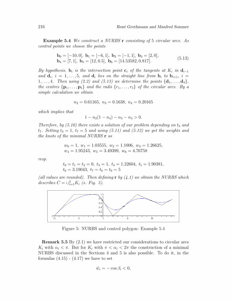
Example 5.4 We construct a NURBS r consisting of 5 circular arcs. Ascontrol points we choose the points

b0 = [−10, 0], b1 = [−6, 1], b2 = [−1, 1], b3 = [2, 0],b4 = [7, 1], b5 = [12, 0.5], b6 = [14.53582, 0.817].

(5.13)

By hypothesis, bi is the intersection point ci of the tangents at Ki in di−1

and di, i = 1, . . . , 5, and di lies on the straight line from bi to bi+1, i =1, . . . , 4. Then using (2.2) and (5.13) we determine the points {d1, . . . ,d4},the centres {p1, . . . ,p5} and the radii {r1, . . . , r5} of the circular arcs. By asimple calculation we obtain

n2 = 0.61165, n3 = 0.1638, n4 = 0.20165

which implies that1− n2(1− n4)− n3 − n4 > 0.

Therefore, by (5.10) there exists a solution of our problem depending on t3 andt7. Setting t3 = 1, t7 = 5 and using (5.11) and (5.12) we get the weights andthe knots of the minimal NURBS r as

w0 = 1, w1 = 1.03555, w2 = 1.1006, w3 = 1.26625,w4 = 1.95243, w5 = 3.49399, w6 = 4.76758

resp.t0 = t1 = t2 = 0, t3 = 1, t4 = 1.22604, t5 = 1.90381,t6 = 3.19043, t7 = t8 = t9 = 5

(all values are rounded). Then defining r by (4.1) we obtain the NURBS whichdescribes C = ∪5

i=1Ki (s. Fig. 5).

Figure 5: NURBS and control polygon: Example 5.4

Remark 5.5 By (2.1) we have restricted our considerations to circular arcsKi with αi < π. But for Ki with π < αi < 2π the construction of a minimalNURBS discussed in the Sections 4 and 5 is also possible. To do it, in theformulas (4.15) - (4.17) we have to set

wi = − cos βi < 0,


where again βi = ^(b2, b0, b1) = ^(di,di−1,bi). Following the arguments in[2] we can then verify that Ki is represented by the weights wi−1 = wi+1 = 1and wi (Ki is the complementary circular arc to the arc with centre angle2π−αi < π represented by the weights wi−1 = wi+1 = 1 and cos βi = −wi > 0).Hence the above discussed construction of a minimal NURBS consisting ofcircular arcs with 0 < αi < 2π, αi 6= π, is possible. This also holds for themethods studied in Section 3. Analogously as above, if αi > π, in (3.4) wehave to set

w2i = 1, i = 0, . . . , L,w2i−1 = − cos ^(b2i,b2i−2,b2i−1) < 0, i = 1, . . . , L.

6 Generalization to Other Types of Conic Sec-

tions

It is well known [2] that every conic section, i.e., an ellipse, a parabola or ahyperbola, can be represented as a rational Bezier-curve of degree two withthe weights wi−1 = wi+1 = 1 and wi 6= 0 (using the notations in Section 4).Specially, if 0 < wi < 1, we have an ellipse, if wi = 1, we obtain a parabola,and for wi > 1, a hyberpola is represented. For the corresponding negativevalues of wi we obtain the complementary conic sections.

Let us now assume that conic sections K1, . . . , KL are given in R2 and sup-pose that there is a tangential transition from Ki to Ki+1 in di where di−1 anddi denote the endpoints of Ki, i = 1, . . . , L. Moreover, let ci be the intersec-tion point of the tangents at Ki in di−1 and di, i = 1, . . . , L. We are interestedin constructing a NURBS r of the type (4.1) which describes the curve

C =L⋃

i=1

Ki.

Following the arguments in Section 4 we define control points {bi}L+1i=0 by

b0 := d0, bi := ci, i = 1, . . . , L, bL+1 := dL.

We still need the weight wi in the representation of Ki as a Bezier-curve of thetype


wi−1B0(t) + wiB1(t) + wi+1B2(t), t ∈ Ii, t ∈ [0, 1],

i = 1, . . . , L (see Section 4, formulas (4.15) and (4.16)).


Then replacing cos βi by wi in (4.19) and in the following arguments weconclude analogously as in Section 5: Defining the values γi, i = 2, . . . , L + 1we can easily verify that Theorem 5.1 characterizes the existence of a minimalNURBS describing C also in the general case.

ACKNOWLEDGEMENT. We want to thank Professor Dr. Wolf Koenigs(chair for history of architecture, emeritus, TU Munic) for many helpful dis-cussions on the volutes at Ionic pillars and other curves in architecture andnature.

References

[1] H. Busing, Vitruvs Volutenrahmen und die System-Konvoluten, JdI, 102(1987), 305 - 338.

[2] G. Farin, Kurven und Flachen im Computer Aided Geometric Design. Einepraktische Einfuhrung, Vieweg Verlag, Braunschweig/Wiesbaden, 1994.

[3] W. Koenigs, Volute - Nautilus - NURBS, to appear in: F. Lang, H. Sven-shon (Eds.), Werkraum Antike, Fs. H. Knell, Darmstadt, 2008.

[4] L. L. Schumaker, Spline Functions: Basic Theory, Wiley-Interscience, NewYork, 1981.

Received: June 1, 2008

composing circular arcs with minimal nurbs · composing circular arcs with minimal nurbs 195...

Documents