1

Comprehensive Modeling Methodologies for NoCRouter Estimation

Andrew B. Kahng Bill Lin Siddhartha Nath

Abstract

Networks-on-Chip (NoCs) are increasingly used in many-core architectures. ORION2.0 [18] is a widely adopted NoC powerand area estimation tool that is based on circuit-level templates, which use specific logic structures to model implementation ofdifferent router components. ORION2.0 estimation models can have large errors (up to 185%) versus actual implementation, oftendue to a mismatch between the actual router RTL and the templates assumed, as well as the effects of optimization tools in moderndesign flows. In this work, we propose comprehensive parametric and non-parametric modeling methodologies that fundamentallydiffer from logic template based approaches in that the estimation models are derived from actual physical implementation data.Specifically, we propose a new parametric modeling methodology as well as improvements to previous work on non-parametricmodeling.

Our work on parametric modeling proposes (1) ORION NEW models, developed using a new methodology that does notassume any logic templates for router components, (2) the use of parametric regression to fit the new models to post-layout powerand area values, and (3) modeling extensions that enable more detailed flit-level power estimation when integrated with simulationtools such as GARNET. The ORION NEW methodology analyzes netlists of NoC routers that have been placed and routed bycommercial tools, and then performs explicit modeling of control and data paths followed by regression analysis to create highlyaccurate NoC models.

Our work on non-parametric modeling expands on our previous work [17] and demonstrates the use of four widely usednon-parametric modeling techniques: Radial Basis Functions, Kriging, Multivariate Adaptive Regression Splines, and SupportVector Machine Regression. The estimation models are also derived from actual physical implementation data. We observe thatnon-parametric modeling techniques have low overhead and complexity of modeling, and are highly accurate.

When compared with actual implementations, our modeling methodologies achieve average estimation errors of no morethan 9.8% across microarchitecture, implementation, and operational parameters as well as multiple router RTL generators. Thesemethodologies are being implemented in an ORION3.0 distribution [19], [66].

I. INTRODUCTION

Networks-on-Chip (NoCs) have proven to be highly scalable and low-latency interconnection fabrics in the era of many-corearchitectures, as evidenced by commercial chips such as the Intel 80-core [63], IBM Blue Gene [64] and Tilera TILE-Gx [65]processors. Because of their growing importance, NoC implementations must be optimized for latency and power [41], [5],[31], [28]. To facilitate early design-space exploration, accurate NoC power and area estimators are required.

One widely adopted approach for NoC power and area estimation, as embodied in ORION2.0 [18], is to develop a logicstructure template for each NoC router component, namely, for the input and output buffers, crossbar, and switch and virtualchannel (VC) arbiters. Despite significant enhancements to improve leakage and clock power modeling, ORION2.0 still produceslarge estimation errors versus actual implementation. This is because there is often a mismatch between the actual RTL and thetemplates assumed. Also, typical design flows involve sophisticated design steps that have complex interactions among them,making their effects difficult to characterize. For example, the crossbar is assumed to have a multiplexer tree structure, and theswitch and VC arbiter is assumed to be a set of NOR and INV gates. However, after logic synthesis and technology mapping,the actual structure can be quite different. For example, AOI instances may be used instead of NOR and INV gates for thearbiter, and tri-state buffers may be used to implement the crossbar. Logic synthesis may also add buffers for performanceoptimizations. These synthesis and other design flow transformations are hard to predict.

An alternative approach is to use parametric regression with high-level analytical models. Although regression analysis isperformed using actual physical implementation data, previous evaluations of this approach [17] show that high-level parametricregression also leads to large estimation errors because important architecture details are often missing in these analytical models.

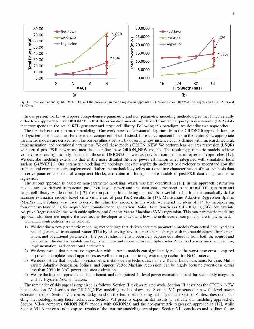
To illustrate the degree of inaccuracy, we show in Figure 1(a) power estimation errors at 65nm for both ORION2.0 and theparametric regression approach based on high-level analytical models, as a function of the number of virtual channels in therouter. The maximum errors are 185% and 75%, respectively. Similarly, in Figure 1(b), we show power estimation errors at90nm when the flit-width is changed.

A. B. Kahng is with the Departments of Computer Science and Engineering, and Electrical and Computer Engineering, University of California at SanDiego, La Jolla, CA 92093-0404. E-mail: abk@ucsd.edu.

B. Lin is with the Department of Electrical and Computer Engineering, University of California at San Diego, La Jolla, CA 92093-0407. E-mail:billlin@eng.ucsd.edu.

S. Nath is with the Department of Computer Science and Engineering, University of California at San Diego, La Jolla, CA 92093-0404. E-mail:sinath@cs.ucsd.edu.

Copyright c© 2011 IEEE. Personal use of this material is permitted. However, permission to use this material for any other purposes must be obtained fromthe IEEE by sending an email to pubs-permissions@ieee.org

2

Fig. 1. Poor estimations by ORION2.0 [18] and the previous parametric regression approach [17]. Netmaker vs. ORION2.0 vs. regression at (a) 65nm and(b) 90nm.

In our present work, we propose comprehensive parametric and non-parametric modeling methodologies that fundamentallydiffer from approaches like ORION2.0 in that the estimation models are derived from actual post place-and-route (P&R) datathat corresponds to the actual RTL generator and target cell library. Following this paradigm, we describe two approaches.

The first is based on parametric modeling. Our work here is a substantial departure from the ORION2.0 approach becauseno logic template is assumed for any router component block. Instead, for each component block in the router RTL, appropriateparametric models are derived from the post-synthesis netlists by observing how instance counts change with microarchitectural,implementation, and operational parameters. We call these models ORION NEW. We perform least-squares regression (LSQR)with actual post-P&R power and area data to refine these ORION NEW models. The resulting parametric models achieveworst-case errors significantly better than those of ORION2.0 as well as previous non-parametric regression approaches [17].We describe modeling extensions that enable more detailed flit-level power estimation when integrated with simulation toolssuch as GARNET [1]. Our parametric modeling methodology does not require the architect or developer to understand how thearchitectural components are implemented. Rather, the methodology relies on a one-time characterization of post-synthesis datato derive parametric models of component blocks, and automatic fitting of these models to post-P&R data using parametricregression.

The second approach is based on non-parametric modeling, which was first described in [17]. In this approach, estimationmodels are also derived from actual post P&R layout power and area data that correspond to the actual RTL generator andtarget cell library. As described in [17], the non-parametric modeling approach is powerful in that it can automatically deriveaccurate estimation models based on a sample set of post P&R results. In [17], Multivariate Adaptive Regression Splines(MARS) linear splines were used to derive the estimation models. In this work, we extend the ideas of [17] by incorporatingfour other metamodeling techniques for automatic model generation: Radial Basis Functions (RBF), Kriging (KG), MultivariateAdaptive Regression Splines with cubic splines, and Support Vector Machine (SVM) regression. This non-parametric modelingapproach also does not require the architect or developer to understand how the architectural components are implemented.

Our main contributions are as follows:1) We describe a new parametric modeling methodology that derives accurate parametric models from actual post-synthesis

netlists generated from actual router RTLs by observing how instance counts change with microarchitectural, implemen-tation, and operational parameters. The post-synthesis netlists accurately capture contributions from both the control anddata paths. The derived models are highly accurate and robust across multiple router RTLs, and across microarchitecture,implementation, and operational parameters.

2) We demonstrate that parametric regression with accurate models can significantly reduce the worst-case error comparedto previous template-based approaches as well as non-parametric regression approaches for NoC routers.

3) We demonstrate that popular non-parametric metamodeling techniques, namely, Radial Basis Functions, Kriging, Multi-variate Adaptive Regression Splines, and Support Vector Machine regression, can be highly accurate (worst-case errorsless than 20%) in NoC power and area estimations.

4) We are the first to propose a detailed, efficient, and fine-grained flit-level power estimation model that seamlessly integrateswith full-system NoC simulators.

The remainder of this paper is organized as follows. Section II reviews related work. Section III describes the ORION NEWmodel. Section IV describes the ORION NEW modeling methodology, and Section IV-C presents our new flit-level powerestimation model. Section V provides background on the four metamodeling techniques, and Section VI describes our mod-eling methodology using these techniques. Section VII presents experimental results to validate our modeling approaches:Section VII-A compares ORION NEW models with ORION2.0 and the non-parametric regression approach in [17], whileSection VII-B presents and compares results of the four metamodeling techniques. Section VIII concludes and outlines future

3

work.

II. RELATED WORK

Previous works have focused primarily on two broad modeling paradigms: (1) architecture-level models using templatesfor each router component block (crossbar, switch and VC arbiter, and input and output buffers), and (2) RTL and gate-level simulation-driven models. For the first approach, Patel et al. [30] propose a transistor count-based analytical modelfor NoC power. Large errors can result because router microarchitectural parameters are not considered. ORION [41] andORION2.0 [18] use microarchitecture and technology parameters for the router component blocks. From our studies as wellas from [17], ORION2.0 estimates have very large errors because the models assume logic template structures for routermicroarchitecture blocks.

The second approach is based on pre-layout (RTL or post-synthesis gate-level) [29], [4], [9], [23] or post-layout [3], [2],[32], [27] simulations. Banerjee et al. [2] report accurate power for a range of routers, but do not present any analytical modelsfor router power. Chan et al. [4] develop cycle-accurate power models with reported average errors up to 20%. Meloni etal. [27] and Lee et al. [23] perform parametric regression analysis on post-layout and RTL simulation results, respectively.Their models are fairly coarse-grained, e.g., they cannot explain sensitivity of power dissipation in each router block to changein load, microarchitecture or implementation parameters.

In the area of flit-level power estimation, Ye et al. [43] and Penolazzi et al. [32] estimate power dissipation using a bit-levelmodel, and Penolazzi et al. [32] propose a static bit-based model to estimate Nostrum NoC power. However, each of thesemodels is tied to a specific router implementation and cannot explain how different bit encodings affect the power consumptionin each block within the router. Our flit-level power estimation methodology estimates the power impact for each componentblock and reports accurate power numbers across different bit encodings in flits.

Non-parametric regression (metamodeling) techniques have been previously used in the field of VLSI and computer ar-chitecture. Ipek et al. [13] use Artificial Neural Networks (ANNs) to predict performance of core and memory in the chip-multiprocessor design space. Kriging (KG) has been widely used for spatial correlation modeling of IR drop and on-chiptemperature [21], as well as estimation of spatial structure of variability sources, and for variability characterization [34]. Leeet al. [25] use KG to automatically search for an optimal microarchitectural design space to estimate tradeoffs in processordesign. Lee et al. [22] use KG to estimate processor power. Multivariate Adaptive Regression Splines (MARS) have been usedto model NoC power and area [17], [14]. Support Vector Machine (SVM) regression has been used in performance modelingof analog circuits [20]. SVM classification has been used for fast simulation of rare circuit events to test SRAM [38]. RadialBasis Functions (RBF) have been used to predict crosstalk in interconnects [12]. We choose to explore RBF, KG, MARS andSVM metamodeling techniques in our work because (1) these methods have been used successfully for estimation purposesin VLSI circuit design, and (2) previous reviews have determined that they are more accurate and robust than other availablenon-parametric modeling techniques [15], [45].

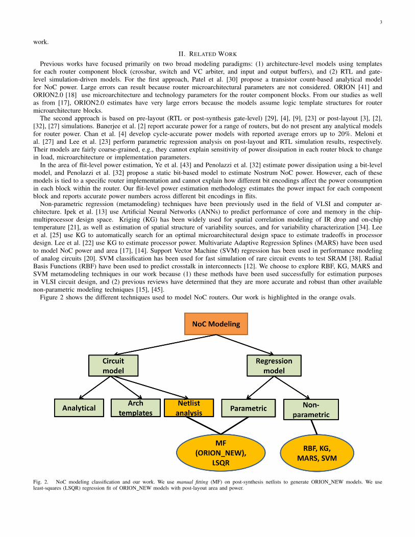
Figure 2 shows the different techniques used to model NoC routers. Our work is highlighted in the orange ovals.

Fig. 2. NoC modeling classification and our work. We use manual fitting (MF) on post-synthesis netlists to generate ORION NEW models. We useleast-squares (LSQR) regression fit of ORION NEW models with post-layout area and power.

4

III. ORION NEW – IMPROVEMENTS TO ARCHITECTURAL MODEL

As shown in Figures 1(a) and (b) of Section I, ORION2.0 [18] and the previous parametric regression techniques [17] havelarge errors compared to implementation. This is because NoC architecture template-based models are incomplete. They do notconsider the impact of frequency scaling, and do not consider more optimized implementations of blocks such as the crossbar.

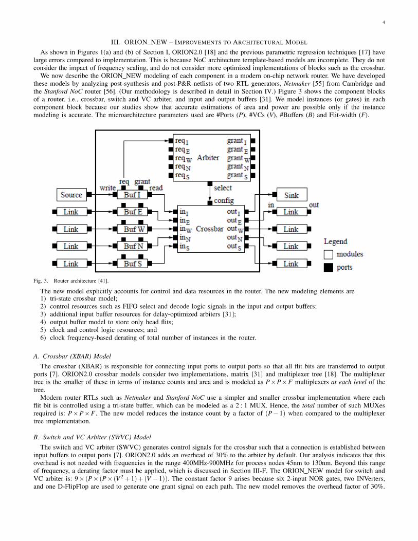
We now describe the ORION NEW modeling of each component in a modern on-chip network router. We have developedthese models by analyzing post-synthesis and post-P&R netlists of two RTL generators, Netmaker [55] from Cambridge andthe Stanford NoC router [56]. (Our methodology is described in detail in Section IV.) Figure 3 shows the component blocksof a router, i.e., crossbar, switch and VC arbiter, and input and output buffers [31]. We model instances (or gates) in eachcomponent block because our studies show that accurate estimations of area and power are possible only if the instancemodeling is accurate. The microarchitecture parameters used are #Ports (P), #VCs (V), #Buffers (B) and Flit-width (F).

Fig. 3. Router architecture [41].

The new model explicitly accounts for control and data resources in the router. The new modeling elements are1) tri-state crossbar model;2) control resources such as FIFO select and decode logic signals in the input and output buffers;3) additional input buffer resources for delay-optimized arbiters [31];4) output buffer model to store only head flits;5) clock and control logic resources; and6) clock frequency-based derating of total number of instances in the router.

A. Crossbar (XBAR) ModelThe crossbar (XBAR) is responsible for connecting input ports to output ports so that all flit bits are transferred to output

ports [7]. ORION2.0 crossbar models consider two implementations, matrix [31] and multiplexer tree [18]. The multiplexertree is the smaller of these in terms of instance counts and area and is modeled as P×P×F multiplexers at each level of thetree.

Modern router RTLs such as Netmaker and Stanford NoC use a simpler and smaller crossbar implementation where eachflit bit is controlled using a tri-state buffer, which can be modeled as a 2 : 1 MUX. Hence, the total number of such MUXesrequired is: P×P×F . The new model reduces the instance count by a factor of (P− 1) when compared to the multiplexertree implementation.

B. Switch and VC Arbiter (SWVC) ModelThe switch and VC arbiter (SWVC) generates control signals for the crossbar such that a connection is established between

input buffers to output ports [7]. ORION2.0 adds an overhead of 30% to the arbiter by default. Our analysis indicates that thisoverhead is not needed with frequencies in the range 400MHz-900MHz for process nodes 45nm to 130nm. Beyond this rangeof frequency, a derating factor must be applied, which is discussed in Section III-F. The ORION NEW model for switch andVC arbiter is: 9× (P× (P× (V 2 +1)+(V −1)). The constant factor 9 arises because six 2-input NOR gates, two INVerters,and one D-FlipFlop are used to generate one grant signal on each path. The new model removes the overhead factor of 30%.

5

C. Input Buffer (InBUF) ModelThe input buffer (InBUF) holds the entire incoming payload of flits at the input stage of the router for decode [7]. ORION2.0

models only the buffer instances and does not take into account control signals which are needed at this stage for decode; theseinclude FIFO select, buffer enable control signals, and logic for housekeeping such as the number of free buffers available perVC, VC identification tag per buffer, etc. As a result, ORION2.0 underestimates the instances at the input stage of the router.

In ORION NEW, we model control signals and housekeeping logic in addition to the actual FIFO buffers. Modern routersimplement the same stage VC and SW allocation to optimize delay [31], leading to doubling of input buffer resources. Hence,in the new model the number of FIFO buffers is 2×P×V ×B×F . The control signals for decoding the housekeeping logicare modeled as: 180×P×V +2×P2×V ×B+3×P×V ×B+5×P2×B+P2 +F ×P+15×P (as analyzed from the post-synthesis and post-P&R netlists). Each constant factor in the model denotes the number of instances per path. For example,the 180 factor accounts for instances to generate FIFO select signals and flags for each buffer in the P×V path. The smallerconstant factors 2, 3 and 5 account for instances that realize local flags in the decode logic. The factor 15 corresponds to thenumber of buffers in each FIFO select path of an input port.

D. Output Buffer (OutBUF) ModelThe output buffer (OutBUF) holds the head flits between the switch and the channel for a switch with output speedup [7].

ORION2.0 models output buffers in exactly the same way as it models input buffers; this is inaccurate for modern routersthat use hybrid output buffers, and leads to an overestimate of the instance count. The output buffers need to store enoughflits to match speeds between the switch and the channel. At the output, these buffers are used to stage the flits between theswitch and channel when channel and switch speeds mismatch. Instead of using P×V ×B×F in ORION2.0, output buffersare proportional to P×V . There are several control signals per port and VC associated with each buffer, which makes theoverall instance counts grow in the new model as P× (80×V +25). The constant factor 80 accounts for the instances used togenerate flow control credit signals for each VC, while the constant factor 25 accounts for buffers and flags.

E. Clock and Control Logic (CLKCTRL) ModelThe clock and control logic (CLKCTRL) models clock buffers and control logic routing resources as clock frequency scales.

ORION2.0 does not model impact on these resources because of frequency scaling. ORION NEW models these resources as2% of the sum of instances in the SWVC, InBUF and OutBUF component blocks.

F. Frequency Derating ModelAs frequency changes, timing constraints change. To meet setup time at higher frequencies, buffers are inserted which leads

to an overall increase in instance counts in the design. ORION2.0 scaling is agnostic to implementation parameters such asclock frequency. This causes large errors in area and instance counts at higher frequencies for component blocks such asSWVC, InBUF and OutBUF. We find that the number of instances in the crossbar does not vary significantly with frequencybecause there are no critical paths; we thus ignore the effects of frequency on the crossbar.

To derate for frequency, we find the frequency below which instance counts change by less than 1%. In 65nm technology,this is 400MHz for both Netmaker and Stanford NoC routers. We derate instance counts by a multiplier ∆Instance that isbased on this frequency as: ∆Instance = ∆Frequency×ConstantFactor. The constant factor depends on the amount of controllogic versus FIFO for each component block. To account for setup buffers, a fitted constant factor of 1 is used in SWVC andInBUF, and a fitted constant factor of 0.03 is used in OutBUF.

IV. ORION NEW METHODOLOGY

In this section, we first describe manual and regression-based methodologies that we use to develop the ORION NEWmodels; we then describe how we estimate power and area using these approaches. We extend our methodology to flit-levelpower estimation in Section IV-C. Key elements of our modeling methodology (see details in Table I) include the following.

• Multiple parametrized NoC RTL generators: Netmaker [55] from Cambridge and the Stanford NoC [56].• Range of values of microarchitecture parameters (#Ports (P), #VCs (V), #Buffers (B) and Flit-width (F)) and implementation

parameters (clock frequency and technology node).• Operational parameters for power calculation: toggle rate1 (TR) and static probability of 1’s in the input (SP).• Multiple commercial tools: Synopsys Design Compiler (DC) [46] and Cadence RTL Compiler (RC) [52], with options to

preserve module hierarchy after synthesis because we analyze each router component block. We compare instance counts,area and power reported by each tool to ensure that for a given RTL these results do not vary by more than 10%.

• Cadence SOC Encounter (SOCE) [53] with die utilization of 0.75 and die aspect ratio of 1.0 to place and route thesynthesized router netlist.

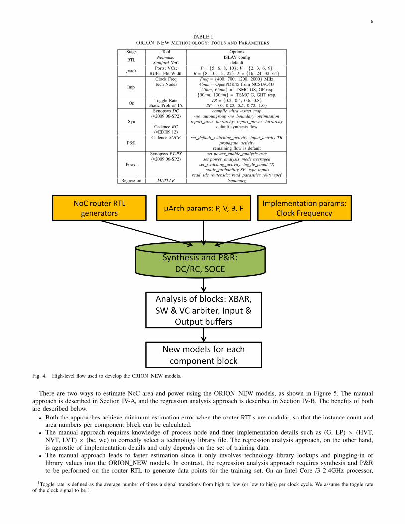
• Synopsys PrimeTime-PX (PT-PX) [47] to run power analysis based on the post-P&R netlist, SPEF [54] and SDC [51].• MATLAB [57] function lsqnonneg for regression analysis.Figure 4 shows the flow we use to develop ORION NEW models for each component block of the router. In Table II, we

summarize the ORION NEW modeling of instance counts of each component block.

6

TABLE IORION NEW METHODOLOGY: TOOLS AND PARAMETERS

Stage Tool Options

RTL Netmaker ISLAY configStanford NoC default

µarch Ports; VCs; P = {5, 6, 8, 10}; V = {2, 3, 6, 9}BUFs; Flit-Width B = {8, 10, 15, 22}; F = {16, 24, 32, 64}

Impl

Clock Freq Freq = {400, 700, 1200, 2000} MHzTech Nodes 45nm = OpenPDK45 from NCSU/OSU

{45nm, 65nm} = TSMC GS, GP resp.{90nm, 130nm} = TSMC G, GHT resp.

Op Toggle Rate TR = {0.2, 0.4, 0.6, 0.8}Static Prob of 1’s SP = {0, 0.25, 0.5, 0.75, 1.0}

Syn

Synopsys DC compile ultra -exact map(v2009.06-SP2) -no autoungroup -no boundary optimization

report area -hierarchy; report power -hierarchyCadence RC default synthesis flow(vEDI09.12)

P&RCadence SOCE set default switching activity -input activity TR

propagate activityremaining flow is default

Power

Synopsys PT-PX set power enable analysis true(v2009.06-SP2) set power analysis mode averaged

set switching activity -toggle count TR-static probability SP -type inputs

read sdc router.sdc; read parasitics router.spefRegression MATLAB lsqnonneg

Fig. 4. High-level flow used to develop the ORION NEW models.

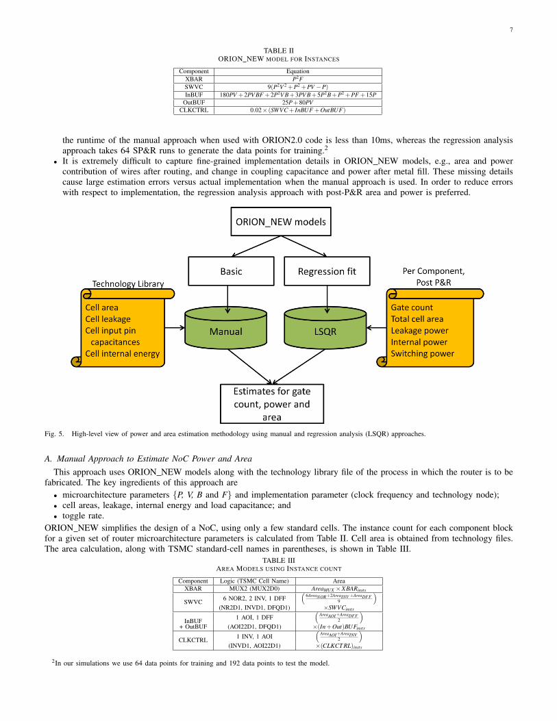
There are two ways to estimate NoC area and power using the ORION NEW models, as shown in Figure 5. The manualapproach is described in Section IV-A, and the regression analysis approach is described in Section IV-B. The benefits of bothare described below.

• Both the approaches achieve minimum estimation error when the router RTLs are modular, so that the instance count andarea numbers per component block can be calculated.

• The manual approach requires knowledge of process node and finer implementation details such as (G, LP) × (HVT,NVT, LVT) × (bc, wc) to correctly select a technology library file. The regression analysis approach, on the other hand,is agnostic of implementation details and only depends on the set of training data.

• The manual approach leads to faster estimation since it only involves technology library lookups and plugging-in oflibrary values into the ORION NEW models. In contrast, the regression analysis approach requires synthesis and P&Rto be performed on the router RTL to generate data points for the training set. On an Intel Core i3 2.4GHz processor,

1Toggle rate is defined as the average number of times a signal transitions from high to low (or low to high) per clock cycle. We assume the toggle rateof the clock signal to be 1.

7

TABLE IIORION NEW MODEL FOR INSTANCES

Component EquationXBAR P2FSWVC 9(P2V 2 +P2 +PV −P)InBUF 180PV +2PV BF +2P2V B+3PV B+5P2B+P2 +PF +15P

OutBUF 25P+80PVCLKCTRL 0.02× (SWVC + InBUF +OutBUF)

the runtime of the manual approach when used with ORION2.0 code is less than 10ms, whereas the regression analysisapproach takes 64 SP&R runs to generate the data points for training.2

• It is extremely difficult to capture fine-grained implementation details in ORION NEW models, e.g., area and powercontribution of wires after routing, and change in coupling capacitance and power after metal fill. These missing detailscause large estimation errors versus actual implementation when the manual approach is used. In order to reduce errorswith respect to implementation, the regression analysis approach with post-P&R area and power is preferred.

Fig. 5. High-level view of power and area estimation methodology using manual and regression analysis (LSQR) approaches.

A. Manual Approach to Estimate NoC Power and AreaThis approach uses ORION NEW models along with the technology library file of the process in which the router is to be

fabricated. The key ingredients of this approach are• microarchitecture parameters {P, V, B and F} and implementation parameter (clock frequency and technology node);• cell areas, leakage, internal energy and load capacitance; and• toggle rate.

ORION NEW simplifies the design of a NoC, using only a few standard cells. The instance count for each component blockfor a given set of router microarchitecture parameters is calculated from Table II. Cell area is obtained from technology files.The area calculation, along with TSMC standard-cell names in parentheses, is shown in Table III.

TABLE IIIAREA MODELS USING INSTANCE COUNT

Component Logic (TSMC Cell Name) AreaXBAR MUX2 (MUX2D0) AreaMUX ×XBARinsts

SWVC 6 NOR2, 2 INV, 1 DFF(

6AreaNOR+2AreaINV +AreaDFF9

)(NR2D1, INVD1, DFQD1) ×SWVCinsts

InBUF 1 AOI, 1 DFF(

AreaAOI +AreaDFF2

)+ OutBUF (AOI22D1, DFQD1) ×(In+Out)BUFinsts

CLKCTRL 1 INV, 1 AOI(

AreaAOI +AreaINV2

)(INVD1, AOI22D1) ×(CLKCT RL)insts

2In our simulations we use 64 data points for training and 192 data points to test the model.

8

Power has three components, that is, leakage, internal and switching. Leakage power is static power when the cell isnot transitioning between logic states. It is dependent on current state of the input pins of the cell as well as process corner,voltage, and temperature. Internal and switching power together constitute dynamic power, which varies with operating voltage,capacitive load and frequency of operation. Internal power is the power dissipated inside a cell and consists of short-circuitpower and switching power of internal nodes; switching power is the power consumed when a load capacitance on a net ischarged and discharged.

In ORION NEW, toggle rate (TR) is equal to the average toggle rate of all input signals in the crossbar, switch and VCarbiter, and control logic in input and output buffers. We assume that buffer cells toggle at 25% of the input toggle rate, sincemultiple VCs do not require buffer contents to change in every cycle.

Leakage power calculation. For leakage power, the model uses the weighted average of the state-dependent leakage of thecells. Equations (1)-(4) are used to calculate the leakage power of each component block.

Pleak XBAR = MUXleak ×XBARinsts (1)

Pleak SWVC =(

6NORleak +2INVleak +DFFleak

9

)×SWVCinsts (2)

Pleak BUF =(

AOIleak +DFFleak

2

)× (In+Out)BUFinsts (3)

Pleak CLKCT RL =(

AOIleak + INVleak

2

)× (CLKCT RL)insts (4)

Internal power calculation. For internal power, table lookups in technology library files return the internal energy of a standardcell given its load capacitance3 and input slew value of ≈ 5×FO4 delay.4 Internal energy is the minimum of the rise and fallenergies. Equations (5)-(8) are used to calculate internal power of each component block.

Pint XBAR = MUXint ×T R×XBARinsts (5)

Pint SWVC = (6NORint +2INVint +DFFint) ×T R×SWVCinsts (6)

Pint BUF = (AOIint +0.25DFFint)×T R × (In+Out)BUFinsts (7)

Pint CLKCT RL = (AOIint + INVint)×T R× (CLKCT RL)insts (8)

Switching power calculation. For switching power, the load capacitance is calculated as the sum of the input capacitancesof pins that are driven by a net and the wire capacitance of the net. The wire capacitance is approximately calculated as aconstant factor times the total pin capacitances. This constant factor is set to 1.4 at 65nm and is assumed to decrease by 14%with each successive process node shrink. Equations (9)-(12) are used to calculate switching power of each component block.

Psw XBAR = XBARload ×T R×XBARinsts (9)

Psw SWVC = SWVCload ×T R×SWVCinsts (10)

Psw BUF = (In+Out)BUFload ×T R × (In+Out)BUFinsts (11)

Psw CLKCT RL = (CLKCT RL)load ×T R× (CLKCT RL)insts (12)

Flow details. The steps below describe how total area and power are estimated using the ORION NEW models and equationsabove.

1) Choose microarchitecture parameters (P, V, B, F), clock frequency, and average toggle rate at inputs.2) Use models in Table II to calculate the instance count of each component block of the router.3) Use models in Table III to calculate the area of each router component block. Total area is calculated as the sum of

areas of all blocks.4) Obtain state-dependent leakage of cells from technology library files. Use Equations (1)-(4) to calculate leakage power

of each component block. Total router leakage power is calculated as the sum of leakage power of all component blocks.5) Obtain internal energy of cells from technology library files. Use Equations (5)-(8) to calculate internal power of each

component block. Total internal power is calculated as the sum of internal power of all component blocks.6) Obtain input pin capacitances of cells from technology library files. Use Equations (9)-(12) to calculate switching power

of each component block. Total switching power is calculated as the sum of switching power of all component blocks.7) The total power dissipated by the router is calculated as the sum of total leakage power, total internal power and total

switching power.

3Load capacitance of a cell depends on its fanout and the cell(s) it drives. We use a fanout of 1. The cells driven depend on the component of the routeras shown in Table III. For example, one DFF drives another DFF and one AOI in the input and output buffers. So, the load capacitance of the DFF is thesum of input pin capacitances of one DFF and one AOI.

4The FO4 delay is the delay of a minimum-sized INV driving four identical INV instances and is a standard proxy for switching speed in a given processtechnology. The resulting slew time values are 80−100ps for 45nm and 65nm technologies.

9

B. Regression Analysis Approach to Estimate NoC Power and AreaAs another approach to estimation of router area and power, we use parametric regression to fit parameters for cell area,

leakage, internal energy, and load capacitance into ORION NEW models. This approach requires instance counts, area, andtotal leakage, internal and switching power of each component block of the router from post-P&R results. Options are set insynthesis tools to preserve module hierarchy and names. Constrained least-squares regression (LSQR) is used to enforce non-negativity of coefficients (cell area, leakage, internal energy, load capacitance). We use the MATLAB [57] function lsqnonnegfor this purpose, and tool options as given in Table I.

Flow Details. LSQR is applied to fit a model of post-P&R instance counts for each router component block. Our training sethas 64 data points. Parametric LSQR is setup as

a1 · Instsmod <component> +a0 = Inststool <component> (13)

where InstsRmod <component> is the refined instance count of each component block after LSQR. The refined instance count is

used to fit models of post-P&R area and power as

b1 · InstsRmod <component> +b0 = Areatool <component> (14)

In Equation (14), b1 is the fitting coefficient for cell area, and the coefficient b0 accounts for the routing overhead.We model leakage, internal and switching power as

{c5, d5, e5} · InstsRmod XBAR + {c4, d4, e4} · InstsR

mod SWVC +

{c3, d3, e3} · InstsRmod InBUF + {c2, d2, e2} · InstsR

mod OutBUF +{c1, d1, e1} · Instsmod CLKCT RL = {Pleak, Pint , Psw}tool

(15)

where coefficients {c5, · · ·,c0} are used to fit cell leakage power, and similarly {d5, · · ·,d0} and {e5, · · ·,e0} are respectivelyused to fit internal energy and load capacitance.

It is possible to skip the instance count refinement step (Equation (14)) and directly perform LSQR for area and leakage,internal, and switching power using the above equations. We observe that average error can change by 3% in either direction byomitting the instance count refinement step. Note that it is necessary to perform per-component LSQR; if LSQR is performedfor the entire router’s area or power, large errors result because multiple components have the same parametric combinationof (P, V, B, F). Failing to separate these contributors to area or power can result in large errors, e.g., at 65nm we haveexperimentally observed worst-case errors of 296% for power and 557% for area. Thus, it is important to preserve modulehierarchy during synthesis in the model development flow.5

C. Extension to Flit-Level Power ModelingThe dynamic power models used in ORION2.0 and ORION NEW do not consider bit encodings in a flit, which can lead to

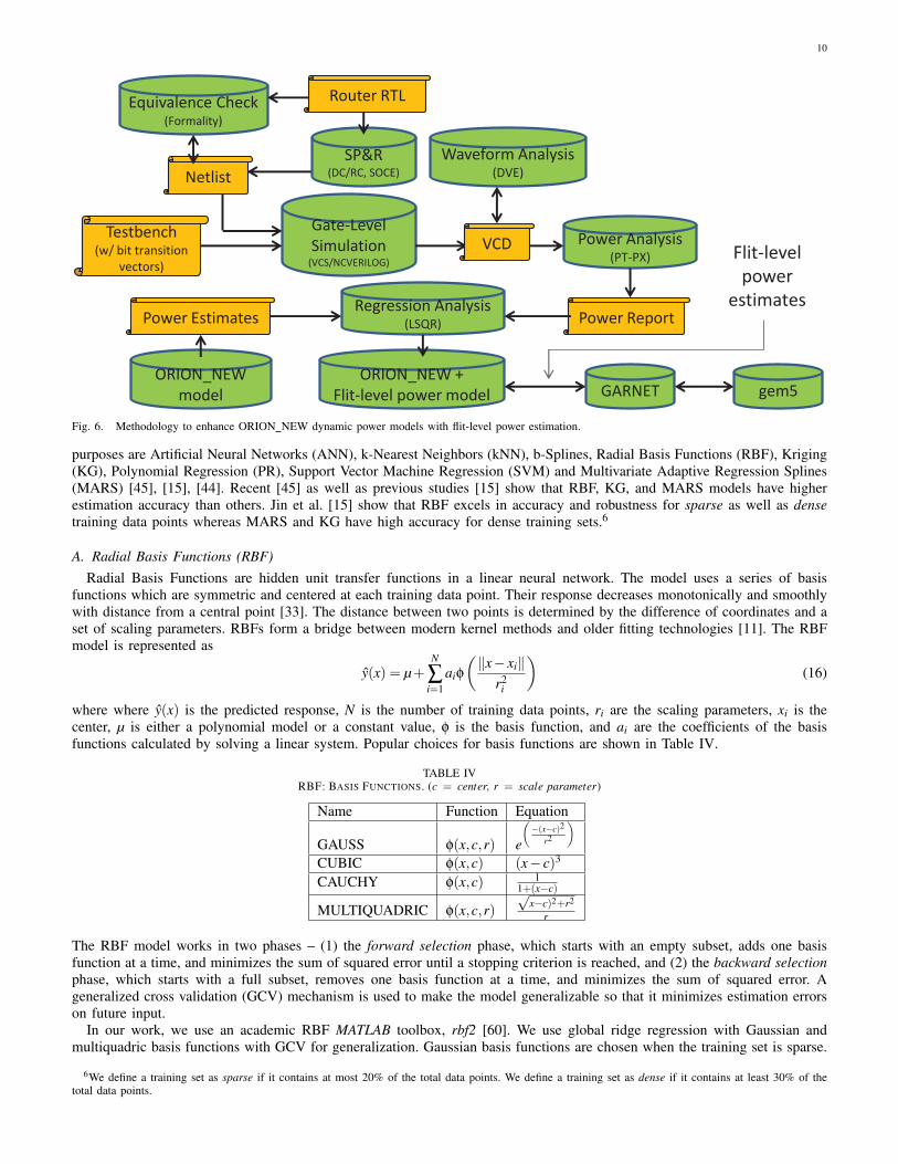
significant errors in dynamic power estimation. As an example, consider two encodings with two consecutive 8-bit flits, whereevery flit has exactly four bits as 1. In the first encoding, the two consecutive flits are 8b′11110000 and 8b′11110000. In thesecond encoding, the two consecutive flits are 8b′11110000 and 8b′00001111. In the first encoding, there are no toggles perconsecutive flits, whereas in the second encoding there are eight toggles per consecutive flits. Clearly, the second encodingwill lead to higher dynamic power than the first one. To model this effect, we use the flow shown in Figure 6. Before usinga testbench, the netlists must pass an equivalence check using tools such as Synopsys Formality [48]. We inject differentbit encodings in the input during simulation over 10000 cycles using GARNET [1], and the resultant VCD (Value ChangeDump) is validated using a waveform analyzer such as Synopsys DVE [49]. A satisfactory VCD is used as input to SynopsysPrimeTime-PX [47] to obtain power values. Regression analysis is performed using the tool-reported power values with theORION NEW estimates to obtain an enhanced ORION NEW model for flit-level power estimation. These models may beinvoked by NoC full-system simulators such as GARNET to obtain very accurate estimates.

V. NON-PARAMETRIC REGRESSION FOR ESTIMATION

Non-parametric regression techniques provide another approach to estimate NoC power and area [17]. Such techniquescan considerably reduce modeling efforts because they require only the microarchitectural, implementation, and operationalparameters as input variables. The models determine the interactions between these input variables and how they affect theoutput (or response). This alleviates the effort needed to model a NoC, as details of architecture-level implementations areavoided. At the same time, non-parametric regression approaches are scalable across multiple router RTLs. We now give abrief background on four widely used non-parametric regression or metamodeling techniques.

Metamodeling techniques can be broadly classified [11] into linear regression-based methods, interpolation-based methods,neural network and kernel-based smoothing methods, and additive tree-based methods. Popular techniques for estimation

5Use of hierarchical synthesis in general leads to lower instance counts, standard-cell area, and total power as compared with flat synthesis results. Thiscomes at the cost of frequency (timing slack), since flat optimization across module boundaries can sometimes achieve better timing results. For our selectionof microarchitecture and implementation parameters, hierarchical synthesis on average has 35% fewer instances, 48.8% less standard-cell area and 49.4% lesstotal power – along with 8% less timing slack – compared with flat synthesis. The runtimes for hierarchical and flat synthesis are within 5% of each other.

10

Netlist

Equivalence Check (Formality)

Testbench (w/ bit transition

vectors)

Gate-Level Simulation

(VCS/NCVERILOG)

SP&R (DC/RC, SOCE)

Waveform Analysis (DVE)

Power Analysis (PT-PX)

Power Report Regression Analysis

(LSQR)

ORION_NEW model

ORION_NEW + Flit-level power model GARNET gem5

Power Estimates

Router RTL

VCD Flit-level power

estimates

Fig. 6. Methodology to enhance ORION NEW dynamic power models with flit-level power estimation.

purposes are Artificial Neural Networks (ANN), k-Nearest Neighbors (kNN), b-Splines, Radial Basis Functions (RBF), Kriging(KG), Polynomial Regression (PR), Support Vector Machine Regression (SVM) and Multivariate Adaptive Regression Splines(MARS) [45], [15], [44]. Recent [45] as well as previous studies [15] show that RBF, KG, and MARS models have higherestimation accuracy than others. Jin et al. [15] show that RBF excels in accuracy and robustness for sparse as well as densetraining data points whereas MARS and KG have high accuracy for dense training sets.6

A. Radial Basis Functions (RBF)Radial Basis Functions are hidden unit transfer functions in a linear neural network. The model uses a series of basis

functions which are symmetric and centered at each training data point. Their response decreases monotonically and smoothlywith distance from a central point [33]. The distance between two points is determined by the difference of coordinates and aset of scaling parameters. RBFs form a bridge between modern kernel methods and older fitting technologies [11]. The RBFmodel is represented as

y(x) = µ+N

∑i=1

aiφ

(‖x− xi‖

r2i

)(16)

where where y(x) is the predicted response, N is the number of training data points, ri are the scaling parameters, xi is thecenter, µ is either a polynomial model or a constant value, φ is the basis function, and ai are the coefficients of the basisfunctions calculated by solving a linear system. Popular choices for basis functions are shown in Table IV.

TABLE IVRBF: BASIS FUNCTIONS. (c = center, r = scale parameter)

Name Function Equation

GAUSS φ(x,c,r) e

(−(x−c)2

r2

)CUBIC φ(x,c) (x− c)3

CAUCHY φ(x,c) 11+(x−c)

MULTIQUADRIC φ(x,c,r)√

x−c)2+r2

r

The RBF model works in two phases – (1) the forward selection phase, which starts with an empty subset, adds one basisfunction at a time, and minimizes the sum of squared error until a stopping criterion is reached, and (2) the backward selectionphase, which starts with a full subset, removes one basis function at a time, and minimizes the sum of squared error. Ageneralized cross validation (GCV) mechanism is used to make the model generalizable so that it minimizes estimation errorson future input.

In our work, we use an academic RBF MATLAB toolbox, rbf2 [60]. We use global ridge regression with Gaussian andmultiquadric basis functions with GCV for generalization. Gaussian basis functions are chosen when the training set is sparse.

6We define a training set as sparse if it contains at most 20% of the total data points. We define a training set as dense if it contains at least 30% of thetotal data points.

11

The scaling parameter (r) also depends on the size of the training set. When the training set is dense, r is chosen to be lessthan 1, whereas when the training set is sparse, 0.5 ≤ r ≤ 2.

B. Kriging (KG)Kriging is a special kind of interpolation function that uses correlation between neighboring points in the training data points

to estimate the response at some other arbitrary point. Kriging models a deterministic response as a realization of a stochasticprocess7

y(x) = f (β,x)+ ε(x) (17)

where f (β,x) expresses the deterministic part of the response, and ε(x) is a random function which expresses the deviationof y(x) from the actual response y. f (β,x) is a linear combination of k known functions and is a realization of a regressionmodel given by

f (β,x) = β1 f1(x)+β2 f2(x)+ · · ·+βk fk(x) (18)

where the coefficients βi, i = 1, ..,k are regression parameters or weights.Once the Kriging model is built, it is used to predict response at arbitrary points which are not in the training data points.

In general, a linear predictor is used [24], i.e.,

y(x) = f (x)Tβ∗+ r(x)T

γ∗ (19)

where β∗ and γ∗ are weights determined from the training data points, f (x)T is the regression model, and r(x)T is the correlationmodel. Linear forms of the regression model are widely used [35] and can be polynomials of order 0 (constant), 1 (linear) or2 (quadratic). Widely used correlation models are one-dimensional [24] and take the form

R(θ,w,x) =N

∏j=1

R j(θ,d j) (20)

where N is the size of the set of training data points, and d j = w j −x j is the deviation between the neighboring points. Somecommon choices of R j(θ,d j) are shown in Table V. In all these models the correlation decreases as |d j| decreases, and largervalues of θ lead to faster decrease.

TABLE VKRIGING: CORRELATION MODELS

Function Name R j(θ,d j)EXP e−θ|d j |

GAUSS e−θd2j

LIN max{0, 1−θ|d j|}SPHERICAL 1−1.5ξ j +0.5ξ j, ξ j =min{1, θ|d j|}CUBIC 1−3ξ2

j +2ξ3j , ξ j =min{1, θ|d j|}

SPLINE 1−15ξ2j +30ξ3

j , if 0 ≤ ξ j ≤ 0.21.25(1−ξ j)3, if 0.2 < ξ j < 10, if ξ j ≥ 1

In our work, we use the KG DACE [24] toolbox for MATLAB [57]. We choose first-order polynomials for the regressionmodel when the training data points are sparse. Higher-order polynomials do not result in a good fit in such cases. Whenthe training set is dense, we use second-order polynomials for regression. We have tried both EXP and GAUSS correlationmodels, as shown in Table V, and have found that EXP gives a fit with smaller Root Mean Square Error (RMSE), Magnitudeof Mean Error (MME) as well as Maximum Error. Area and power are not smooth functions for higher-order differentials [24]and exhibit a linear behavior near the origin. The EXP models also have this behavior, whereas GAUSS is parabolic near theorigin. We make an initial guess on θ to be 40 and then allow the model to change it during the fitting process.

C. Multivariate Adaptive Regression Splines (MARS)Multivariate Adaptive Regression Splines is a flexible regression modeling technique for high-dimensional input data, that

is, for a large number of input variables [11]. The model is a product of spline basis functions, and is constructed using aniterative forward and backward approach. The number of basis functions, product degree, and knot8 locations are determinedautomatically using the training data points during iterative steps. The MARS model is represented as a sum of basis functions

y(x) = c0 +I

∑i=1

ci fi(x) (21)

7Least squares regression (LSQR) fit assumes the residue to have Gaussian distribution with zero mean and constant variance, whereas Kriging models theresidue as a stochastic process [21]. This allows Kriging to reduce the estimation error better than LSQR.

8Knot is the value of an input parameter that causes a piecewise line segment to changes its slope.

12

where I is the number of basis functions besides the constant basis function f0(x) = 1, c0 is the coefficient of the constantbasis function, and ci are the coefficients of each of the I basis functions. These basis functions are of the form

fi(x) =Ji

∏j=1

[b ji

(xv( j,i)− t ji

)]+ (22)

where J is the number of input variables, Ji is the number of interactions between variables in the ith basis function, b ji =±1,xv( j,i) is the vth input variable, 1≤ v( j, i)≤ J, t ji is the knot location on each of the corresponding variables, and the subscript”+” denotes the positive part of a truncated power function.

MARS works in two passes. The forward pass starts with a knot, then basis functions are repeatedly added in pairs tothe model until the number of added basis functions reaches I, which is an input to the model. The forward pass usuallyresults in an overfit, so it is followed by a backward pass that prunes the model with better ability to generalize using a GCVmechanism [8], given by

GCV (M) =1N

N

∑p=1

[yp− y(xp)]2

[1− C(M)

N

]2 (23)

where N is the number of training data points, yp is the actual response, y(xp) is the predicted response for the input xp, Mis the number of non-constant basis functions, and C(M) is the complexity penalty to avoid overfitting and is typically thenumber of parameters being fitted. The GCV criterion is a mean squared residual fit to the training data times a penalty toaccount for the increased variance associated with increasing model complexity.

In our work, we use an academic MARS MATLAB toolbox, ARESLab [58].9 We use both cubic as well as linear splines tofit the training data points. As indicated in Table VI below, for all sizes of the training data set, we set the maximum numberof basis functions to 50 and the maximum degree of interactions between input variables to three. There are four variables(P, V, B, F) in the input, and the maximum degree of interactions is typically chosen to be one less than the number of inputvariables [14].

D. Support Vector Machine Regression (SVM)Regression based on Support Vector Machine is an adaptation of the popular SVM classification model [11], [39], [10]. The

objective is to minimize a loss function such as, Huber, ε-insensitive, or quadratic. The SVM model can be represented as [11]

y(x) = c0 +M

∑i=1

cihi(x) (24)

where c0 and ci are coefficients to be determined by minimizing the loss function, hi are the basis functions, and M is themaximum number of basis functions added by the kernel method. We use the Huber loss function [10]

LHuber(y(x)− y) =

{12 (y(x)− y)2 if |y(x)− y| ≤ µ

µ|y(x)− y|− µ2

2 otherwise(25)

where µ is a pre-chosen error bound. To determine the coefficients of the basis functions, the following function is minimized

min.M

∑i=1

LHuber(y(x)− y)+C2‖ci‖ (26)

where C is a pre-chosen cost penalty.In our work, we use the LIBSVM [61] toolbox for MATLAB. We use the Huber loss function as the optimal regression

function to minimize the mean squared error of the model. We set the cost parameter as the maximum difference of theresponses in the training data points, and we use RBF as the kernel method to generate basis functions as shown in Table VI.

VI. METAMODELING METHODOLOGY

We now describe how we use the metamodeling techniques described in Section V to estimate NoC area and power. We firstperform synthesis using Synopsys Design Compiler [46], followed by place and route using Cadence SOC Encounter [50],of the Netmaker [55] router RTL. Next, we generate area and power reports of these designs to use as training and test datapoints. Figure 7 shows our synthesis and P&R flow, Table I lists the architecture, implementation, and operational parameters,and Table VI lists the tool options used in our experiments. We generate 256 data points for our experiments. We use twosampling methodologies to generate the training sets – a modified Latin Hypercube Sampling (LHS) [15], and a restrictedsampling methodology which samples only values from the lower ranges of the parameters (B, V, P, F). Our LHS methodology(for 64 data points of four variables) is as follows.

9We compared results of ARESLAB with a commercial MARS tool from Salford Systems [59] and found that estimation errors of both these tools aresimilar.

13

1) Generate 64 normalized LHS samples over four parameters using the MATLAB command lhsdesign(64, 4).2) Maximize the minimum distance between samples by using the MATLAB command bsxfun [62].3) Map the samples generated in the previous step to our ranges of B, V, P and F parameters by selecting the value which

is closest to the sample.4) Adjust the frequency of the values to make the samples uniformly distributed across our range of values for B, V, P and

F so that each of them occurs the same number of times in the training set.The restricted sampling methodology does not include higher values of the microarchitectural parameters in the training set.

More precisely, the resulting training sets omit all values of {B=7}, or of {P = 9}, or of {V = 7}, or of {F = 64}.Unlike previous approaches using MARS [17], we model leakage, internal, and switching power separately. This results in

more accurate fit of the training data because each of these components of power does not change in the same fashion withmicroarchitectural, implementation, and operational parameters. Figure 8 shows the flow of our methodology.

Fig. 7. Implementation flow to generate training and test data points.

Fig. 8. Area and power modeling and prediction flow.

We assess the goodness of fit of RBF, KG, MARS and SVM models using three metrics.• Magnitude of Mean Error (MME): This is the mean of the magnitude of errors at each predicted output using the test

data points.• Root Mean Square Error (RMSE): This is the square root of the mean of the sum of squared error for the predicted

outputs using the test data points.

14

TABLE VIMETAMODELING METHODOLOGY: TOOLS AND PARAMETERS

Stage Tool Values

LHS MATLAB lhsdesignbsxfun

KG DACE Reg model = {Order 1 and 2 Poly}Corr model = {EXP, GAUSS}, θ = {40}

RBFRBF2 Type = {Ridge Regression}

Func. Type = {GAUSS, MULTIQUADRIC}2 ≤ r ≤ 0.5

MARSARESLAB Max Basis Funcs = {50}

Max Interactions = {3}Spline Type = {linear, cubic}

SVM LIBSVM Type = {nu-SVR}v3.12 Kernel = {RBF}

• Maximum Error (MAXE): This is the maximum of the magnitude of errors at each predicted output using the test datapoints. We include this metric to give a sense of the worst-case error, which is of practical concern for hardware designersand computer architects.

VII. VALIDATION AND RESULTS

In this section, we discuss our validation and results of (1) ORION NEW, (2) ORION NEW with parametric regression, and(3) metamodeling techniques. We calculate the magnitude of percentage estimation error as Error% = ABS((TOOL − MODEL) / MODEL × 100).

A. Results of ORION NEWWe set up experiments as described in Table I of Section IV. We use parameters and tools for our experiments as listed in

Table I. We discuss the results in two parts, (1) ORION2.0 versus ORION NEW estimation of area and power, and (2) impactof our regression analysis approach versus the approach used in prior work of [17]. Comparisons are made with respect topost-P&R instance counts, power and area outcomes, and both router RTL generators, Netmaker [55] and Stanford NoC [56].

1) ORION2.0 versus ORION NEW Comparisons. Since the instance counts per component are at the core of the ORION NEWmodel, we compare ORION2.0 estimates of instance (or gate) counts, as well as the ORION NEW model estimates, withimplementation (post-P&R) for each component block. Figures 9(a), 10(a), and 11(a) show the large errors in ORION2.0for crossbar, output buffer and input buffer respectively, and Figures 9(b), 10(b), and 11(b) show the significant reductionin estimation errors for these components with ORION NEW models. ORION2.0 and ORION NEW are plotted in differentgraphs because of the large errors in instance counts for ORION2.0.

Fig. 9. (a) XBAR with #ports: ORION2.0 vs. im-plementation. (b) XBAR with #ports: ORION NEWvs. implementation.

Fig. 10. (c) Output buffer with #VCs: ORION2.0vs. implementation. (d) Output buffer with #VCs:ORION NEW vs. implementation.

Fig. 11. (e) Input buffer with flit-width: ORION2.0vs. implementation. (f) Input buffer with flit-width:ORION NEW vs. implementation.

ORION2.0 modeling of instance counts for a component does not consider implementation parameters such as clockfrequency. As a result, the instance counts do not scale when frequency is changed, even though at higher frequencies buffersare typically inserted to meet tight setup time constraints. Our ORION NEW models apply a frequency derating factor tothe instance models for component blocks as described in Section III-F. Figures 12(a) and (b) respectively show results foroutput and input buffer component blocks; the incorrect estimates by ORION2.0 contrast sharply with the estimates fromORION NEW, which are very close to actual implementation.

Table 13 summarizes ORION2.0 and ORION NEW estimation errors with respect to Netmaker and Stanford NoC post-P&Rarea. Higher error values are highlighted in red. Figures 14(a) and (b) plot the estimation errors for power and area respectively

15

Fig. 12. (a) Output buffer with clock frequency: ORION2.0 vs. ORION NEW. (b) Input buffer with clock frequency: ORION2.0 vs. ORION NEW.

Component Avg Error: #Instances

Max Error: #Instances

Avg Error: Total Area

Max Error: Total Area

2.0 NEW 2.0 NEW 2.0 NEW 2.0 NEW

XBAR 86.10% 2.10% 93.10% 3.00% 86.20% 0.90% 93.20% 1.80%

SWVC 12.30% 12.30% 35.40% 35.40% 15.90% 20.80% 39.10% 66.80%

InBUF 270.70% 8.00% 417.30% 19.30% 134.40% 6.50% 199.40% 20.20%

OutBUF 69.00% 13.60% 80.60% 27.80% 74.70% 24.80% 86.40% 60.10%

Overall 109.50% 8.80% 156.60% 21.40% 77.80% 13.30% 104.50% 37.20%

Fig. 13. Instance counts and area error comparison of ORION2.0 vs. ORION NEW.

at 45nm and 65nm technology nodes after applying the regression fitting approach described in Section IV-B. We see thatORION NEW estimates are very close to actual implementation (average error of 9.8% in estimating Netmaker power at45nm) and are robust across multiple microarchitecture, implementation parameters, and router RTLs.

Next, we analyze the impact of flit-level power modeling as described in Section IV-C. To capture the effect of runningsimulations with input vectors having different bit encodings (shown in Figure 6), we use options in Synopsys PrimeTime-PX [47] to vary toggle rates and bit encodings in the input. We run simulations using four different toggle rates (0.2, 0.4,0.6, and 0.8) and four different encodings of 1’s in 32-bit input flits. We observe that leakage power is not dependent on bitencodings (changes by less than 2%). However, dynamic power varies by up to 30% (on average) depending on bit encodingsin each flit. ORION2.0 models are incomplete because they consider only the flit arrival rates in the dynamic power estimationmodels. Figure 15 compares dynamic power estimation error of ORION2.0, ORION NEW, and ORION NEW with flit-levelpower models. We observe that by using flit-level power models, average dynamic power estimation error can be within 12%.

2) Impact of our regression analysis approach. In Section IV-B, we describe our parametric regression analysis approachusing the ORION NEW models. As seen from the above results (Section VII-A1), the ORION NEW models are accurateacross microarchitecture, implementation, and operational parameters. With these accurate models, regression analysis canminimize errors and generate accurate fitting coefficients. The previous parametric regression approach [17] reports largeerrors because underlying ORION2.0 models do not model control path elements. The non-parametric regression approachof [17] using MARS achieves reduced average power modeling errors of 5.82% at 65nm and 5.65% at 90nm, and reducedaverage area errors of 5.41% at 65nm and 5.01% at 90nm. In our work, we use parametric regression analysis but with accurateORION NEW models. Our average errors are similar to [17]; however, our maximum error for power (resp. area) is reducedfrom 59.41% to 24.42% (resp. from 61.84% to 30.30%) at 65nm. At 90nm the reduction of maximum power (resp. area) erroris from 60.15% to 28.04% (resp. from 60.07% to 19.36%). The reduction of maximum estimation error is significant becauseNoC designers and architects care about worst-case accuracy.

16

(a)

(b)

0%

20%

40%

60%

80%

100%

NEW 2.0 NEW 2.0 NEW 2.0 NEW 2.0

45nm 65nm 45nm 65nm

Stanford NoC NetMaker

Avg

Max

Min

0%

20%

40%

60%

80%

100%

NEW 2.0 NEW 2.0 NEW 2.0 NEW 2.0

45nm 65nm 45nm 65nm

Stanford NoC NetMaker

Avg

Max

Min

Fig. 14. ORION NEW with regression fit vs. ORION2.0: (a) power estimation error and (b) area estimation error.

B. Results of Metamodeling TechniquesWe set up experiments for each of the metamodeling techniques using the parameters, tools, and methodology as described

in Table VI and Section VI. We generate 256 data points of post-P&R power and area values using 45nm and 65nm technologylibraries. The input variables to all the models are P, V, B and F and the responses are post-P&R power and area. We use thesampling methodology described in Section VI to generate training sets of three sizes.

• 50 data points – sparse and restricted,• 64 data points – sparse, and• 102 data points – dense.

We use the sparse and restricted training set to test the accuracy of models in estimating area and power for input parameterswhich are beyond the range of values used for training. In each experiment, model generation takes around 3s and responseestimation takes around 1.88s. We repeat all experiments 10 times for each training set size, and report the averages of all theerror values across the 10 trials.

We present the results of metamodeling techniques as (1) comparisons among the techniques used, (2) comparisons againstMARS with linear splines [17], and (3) comparisons against parametric regression techniques [16].

1) Metamodeling accuracy. Figures 16(a) and (b) show the percentage errors observed in estimating standard-cell area at65nm and 45nm. With a dense training set, RBF, KG and MARS have similar maximum estimation errors of around 20%.SVM, on the other hand, has maximum estimation errors of 37.8% at 45nm and 25% at 65nm. The average estimation errorsof all these models are less than 10.7%, with SVM having higher average estimation error than RBF, KG and MARS. With asparse training set (64 data points), RBF and KG have higher accuracies than MARS and SVM. RBF always performs betterthan KG, MARS, and SVM with a sparse and restricted training set (50 data points). Figure 16(b) shows that with a sparse and

17

0%

20%

40%

60%

80%

Flit-Level NEW 2.0 Flit-Level NEW 2.0

Stanford NoC NetMaker

Avg

Max

Min

Fig. 15. Comparison of dynamic power estimation error using (1) ORION2.0, (2) ORION NEW, and (3) ORION NEW with flit-level power models.

restricted training set the maximum estimation error is less than 12.8% for RBF, whereas the maximum estimation errors aremore than 32% for KG, MARS, and SVM. The accuracies of these models in estimating power are similar to their accuraciesin estimating area, as shown in Figures 17(a) and (b). With a sparse and restricted training set, RBF can be three times moreaccurate than KG, SVM and MARS. RBF and KG have similar errors for sparse as well as dense training sets. Across alltraining set sizes used in our experiments, we observe that area and power estimation errors are the smallest for RBF and arethe highest for SVM.

Fig. 16. Area estimation accuracy of metamodelingtechniques at (a) 65nm and (b) 45nm.

Fig. 17. Power estimation accuracy of metamodel-ing techniques at (a) 65nm and (b) 45nm.

Fig. 18. Comparison with estimation errors of [17]at 65nm: (a) area, and (b) power. Minimum errorsare too small to appear in the plot.

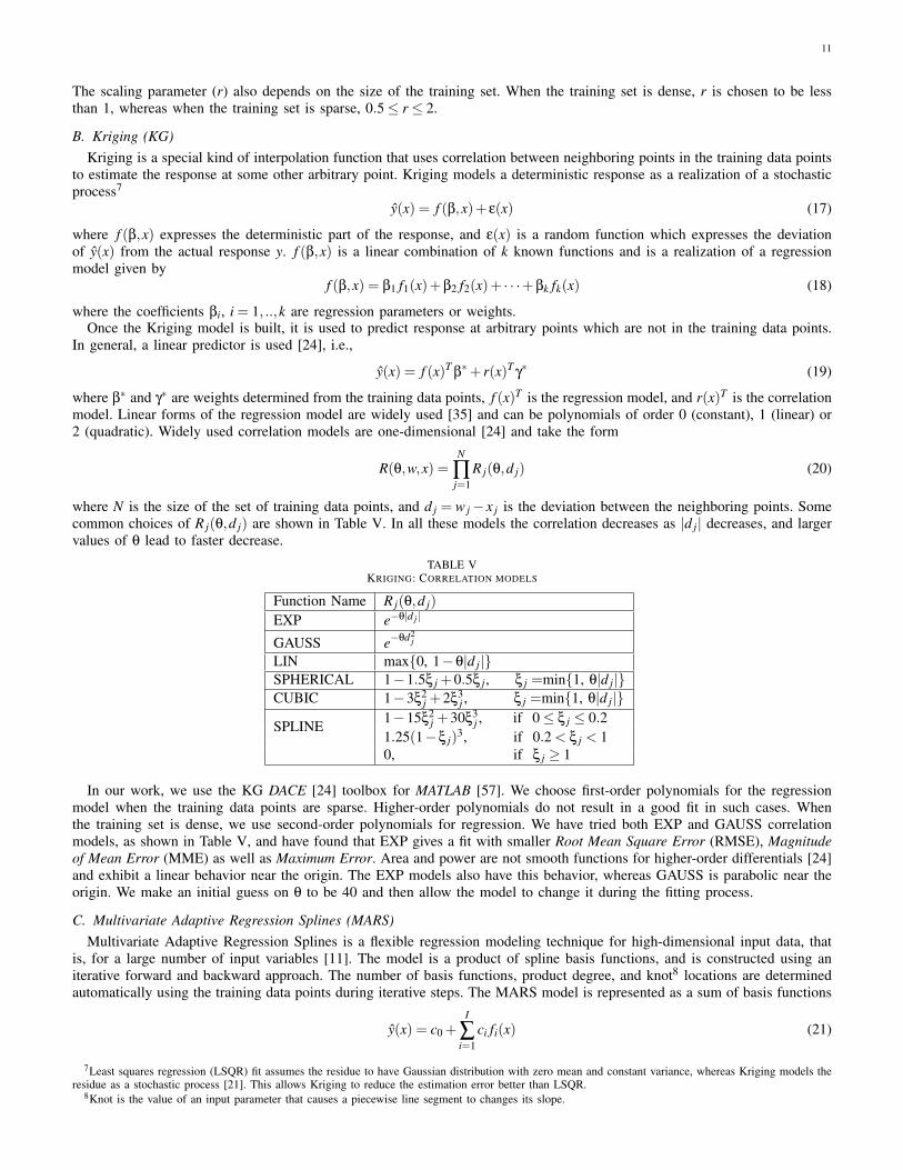
2) Comparison of MARS linear and cubic splines. Prior work in [17] uses MARS with linear splines to model NoC area andpower, and reports maximum estimation errors of around 60% at 65nm. We use MARS with cubic splines in our experiments.Figures 18(a) and (b) compare area and power at 65nm with our metamodeling techniques. In general, our maximum estimationerrors are smaller than those of [17] across all the techniques. In particular, our estimation errors (maximum, average andminimum) for MARS are smaller than in [17]; this is because cubic splines are better than linear splines in minimizingestimation errors. Figures 19(a) and (b) show that cubic splines perform better than linear splines across different technologiesand training set sizes. With a sparse training set at 65nm, the maximum area (resp. power) estimation error is 24.8% (resp.19.7%) with cubic splines, whereas it is 33.6% (resp. 28.3%) with linear splines.

3) Comparison with parametric regression. We use a sparse training set of 64 data points to estimate area and power using theparametric LSQR technique used to fit parametric models of router component blocks in [16]. Figures 20(a) and (b) compare

18

Fig. 19. MARS linear vs. cubic splines: (a) powerand (b) area.

Fig. 20. Comparison of estimation errors of non-parametric vs. parametric regression techniques: (a)area and (b) power.

Fig. 21. Comparison of estimation error in flit-level power modeling at 65nm: (a) maximum and(b) average.

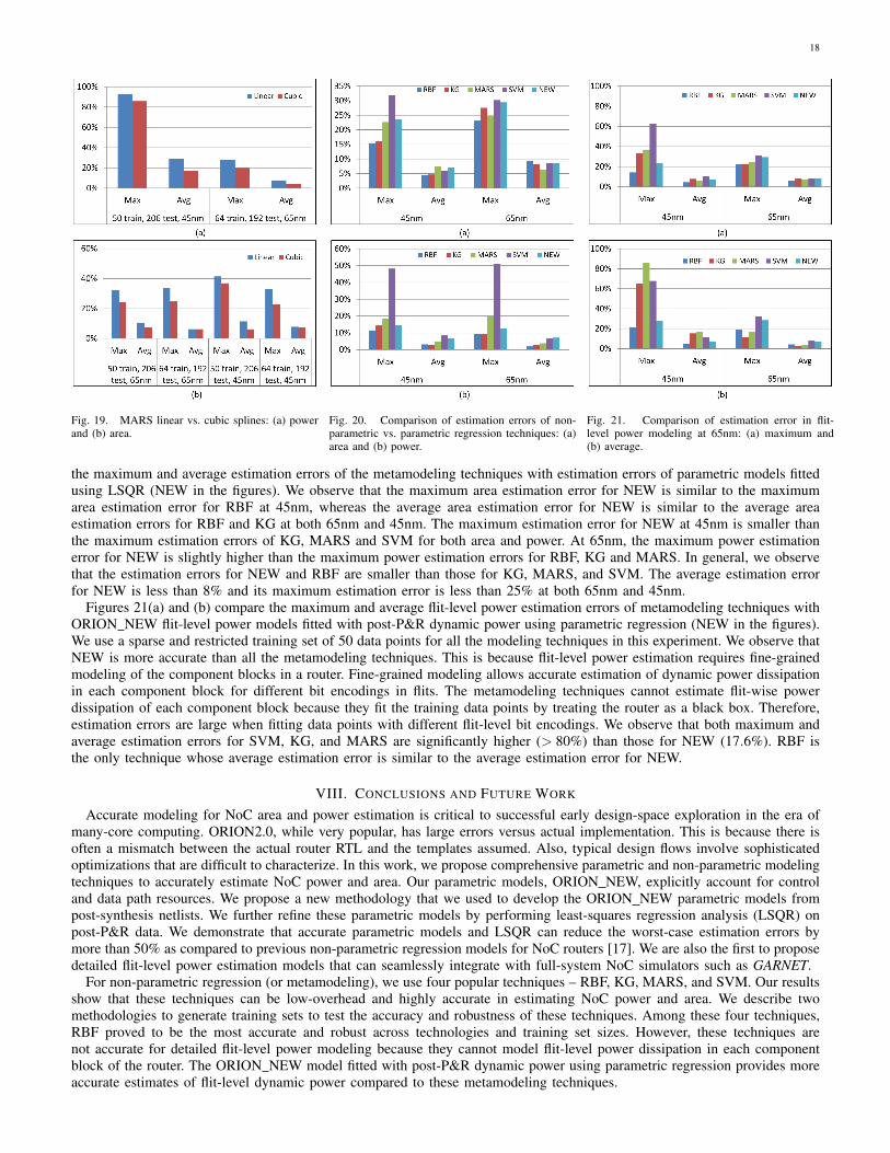
the maximum and average estimation errors of the metamodeling techniques with estimation errors of parametric models fittedusing LSQR (NEW in the figures). We observe that the maximum area estimation error for NEW is similar to the maximumarea estimation error for RBF at 45nm, whereas the average area estimation error for NEW is similar to the average areaestimation errors for RBF and KG at both 65nm and 45nm. The maximum estimation error for NEW at 45nm is smaller thanthe maximum estimation errors of KG, MARS and SVM for both area and power. At 65nm, the maximum power estimationerror for NEW is slightly higher than the maximum power estimation errors for RBF, KG and MARS. In general, we observethat the estimation errors for NEW and RBF are smaller than those for KG, MARS, and SVM. The average estimation errorfor NEW is less than 8% and its maximum estimation error is less than 25% at both 65nm and 45nm.

Figures 21(a) and (b) compare the maximum and average flit-level power estimation errors of metamodeling techniques withORION NEW flit-level power models fitted with post-P&R dynamic power using parametric regression (NEW in the figures).We use a sparse and restricted training set of 50 data points for all the modeling techniques in this experiment. We observe thatNEW is more accurate than all the metamodeling techniques. This is because flit-level power estimation requires fine-grainedmodeling of the component blocks in a router. Fine-grained modeling allows accurate estimation of dynamic power dissipationin each component block for different bit encodings in flits. The metamodeling techniques cannot estimate flit-wise powerdissipation of each component block because they fit the training data points by treating the router as a black box. Therefore,estimation errors are large when fitting data points with different flit-level bit encodings. We observe that both maximum andaverage estimation errors for SVM, KG, and MARS are significantly higher (> 80%) than those for NEW (17.6%). RBF isthe only technique whose average estimation error is similar to the average estimation error for NEW.

VIII. CONCLUSIONS AND FUTURE WORK

Accurate modeling for NoC area and power estimation is critical to successful early design-space exploration in the era ofmany-core computing. ORION2.0, while very popular, has large errors versus actual implementation. This is because there isoften a mismatch between the actual router RTL and the templates assumed. Also, typical design flows involve sophisticatedoptimizations that are difficult to characterize. In this work, we propose comprehensive parametric and non-parametric modelingtechniques to accurately estimate NoC power and area. Our parametric models, ORION NEW, explicitly account for controland data path resources. We propose a new methodology that we used to develop the ORION NEW parametric models frompost-synthesis netlists. We further refine these parametric models by performing least-squares regression analysis (LSQR) onpost-P&R data. We demonstrate that accurate parametric models and LSQR can reduce the worst-case estimation errors bymore than 50% as compared to previous non-parametric regression models for NoC routers [17]. We are also the first to proposedetailed flit-level power estimation models that can seamlessly integrate with full-system NoC simulators such as GARNET.

For non-parametric regression (or metamodeling), we use four popular techniques – RBF, KG, MARS, and SVM. Our resultsshow that these techniques can be low-overhead and highly accurate in estimating NoC power and area. We describe twomethodologies to generate training sets to test the accuracy and robustness of these techniques. Among these four techniques,RBF proved to be the most accurate and robust across technologies and training set sizes. However, these techniques arenot accurate for detailed flit-level power modeling because they cannot model flit-level power dissipation in each componentblock of the router. The ORION NEW model fitted with post-P&R dynamic power using parametric regression provides moreaccurate estimates of flit-level dynamic power compared to these metamodeling techniques.

19

We validate robustness of our modeling methodologies across multiple router RTLs, and across microarchitecture, imple-mentation, and operational parameters. We conclude that our modeling methodologies are highly accurate with average errors≤ 9.8%. Implementations of our modeling methodologies are being made available for download in an ORION3.0 distribution[19], [66]. We plan to extend our work to accurately model link power by incorporating link signaling elements such asdifferential signaling, scrambling, serdes, equalization and 3D routing.

ACKNOWLEDGMENTS

This work was supported in part by the National Science Foundation (NSF) under grant number SHF-1116667. The authorsacknowledge the support of the Gigascale Systems Research Center (GSRC), one of the six research centers funded under theFocus Center Research Program (FCRP), a Semiconductor Research Corporation entity.

REFERENCES

[1] N. Agarwal, T. Krishna, L.-S. Peh and N. K. Jha, “GARNET: A detailed on-chip network model inside a full-system simulator”, Proc. ISPASS, 2009,pp. 33-42.

[2] A. Banerjee, R. Mullins and S. Moore, “A power and energy exploration of network-on-chip architecture”, Proc. NOCS, 2007, pp. 163-172.[3] N. Banerjee, P. Vellanki and K. S. Chatha, “A power and performance model for network-on-chip architectures”, Proc. DATE, 2004, pp. 1250-1255.[4] J. Chan and S. Parameswaran, “NoCEE: Energy macro-model extraction methodology for network-on-chip routers”, Proc. ICCAD, 2005, pp. 254-259.[5] K. Chang, J. Shen and T. Chen, “A low-power crossroad switch architecture and its core placement for network-on-chip”, Proc. DATE, 2005, pp. 375-380.[6] W. J. Dally and B. Towles, “Route packets not wires: On-chip interconnection networks”, Proc. DAC, 2001, pp. 684-689.[7] W. J. Dally and B. Towles, Principles and practices of interconnection networks, Morgan Kaufmann, 2004.[8] J. H. Friedman, “Multivariate adaptive regression splines”, The Annals of Statistics 19(1) (1991), pp. 1-141.[9] G. Guindani, C. Reinbrecht, T. Raupp, N. Calazans and F. G. Moraes, “NoC power estimation at the RTL abstraction level”, Proc. ASVLSI, 2008, pp.

475-478.[10] S. R. Gunn, “Support vector machines for classification and regression”, University of Southampton Technical Report, 1998.[11] T. Hastie, R. Tibshirani and J. Friedman, The elements of statistical learning: Data mining, inference, and prediction, Springer, 2009.[12] A. A. Ilumoka, “Efficient prediction of crosstalk in VLSI interconnects using neural networks”, Proc. EPEP, 2000, pp. 87-90.[13] E. Ipek, S. A. McKee, B. R. de Supinski, M. Schulz and R. Caruana “Efficiently exploring architectural design spaces via predictive modeling”, Proc.

ASPLOS, 2006, pp. 195-206.[14] K. Jeong, A. B. Kahng, B. Lin and K. Samadi, “Accurate machine learning-based on-chip router modeling”, IEEE ESL, 2(3) (2010), pp. 62-66.[15] R. Jin, W. Chen and T. W. Simpson, “Comparative studies of metamodeling techniques under multiple modeling criteria”, Trans. Struct. Multidiscip.

Optim. 23 (2001), pp. 1-13.[16] A. B. Kahng, B. Lin and S. Nath, “Explicit modeling of control and data for improved NoC router estimation” Proc. DAC, 2012, pp. 392-397.[17] A. B. Kahng, B. Lin and K. Samadi, “Improved on-chip router analytical power and area modeling” Proc. ASPDAC, 2010, pp. 241-246.[18] A. B. Kahng, B. Li, L.-S. Peh and K. Samadi, “ORION 2.0: A fast and accurate NoC power and area model for early-stage design space exploration”,

Proc. DATE, 2009, pp. 423-428.[19] A. B. Kahng, B. Lin and S. Nath, “Comprehensive modeling methodologies for NoC router estimation”, University of California San Diego Technical

Report CS2012-0989, 2012, pp. 1-14.[20] T. Kiely and G. Gielen, “Performance modeling of analog integrated circuits using least-squares support vector machines”, Proc. DATE, 2004, pp.

448-453.[21] F. Liu, “A general framework for spatial correlation modeling in VLSI design”, Proc. DAC, 2007, pp. 817-822.[22] B. C. Lee and D. M. Brooks, “Accurate and efficient regression modeling for microarchitectural performance and power prediction”, Proc. ASPLOS,

2006, pp. 185-194.[23] S. E. Lee and N. Bagherzadeh, “A high level power model for network-on-chip (NoC) router”, Integration, the VLSI journal 35(6) (2009), pp. 1-7.[24] S. N. Lophaven, H. B. Nielsen and J. Sondergaard, “Aspects of the MATLAB toolbox DACE”, Technical University of Denmark Technical Report

IMM-REP-2002-13, 2002.[25] G. Mariani, A. Brankovic, G. Palermo, J. Jovic, V. Zaccaria and C. Silvano, “A correlation-based design space exploring methodology for multi-processor

systems-on-chip”, Proc. DAC, 2010, pp. 120-125.[26] G. Mariani, G. Palermo, V. Zaccaria and C. Silvano, “OSCAR: An optimization methodology exploiting spatial correlation in multicore design spaces”,

IEEE Trans. CAD 31(5) (2012), pp. 740-753.[27] P. Meloni, I. Loi, F. Angiolini, S. Carta, M. Barbaro, L. Raffo and L. Benini, “Area and power modeling for network-on-chip with layout awareness”,

Proc. IEEE VLSI Design, 2007, pp. 1-12.[28] R. Mullins, A. West and S. Moore, “The design and implementation of a low-latency on-chip network”, Proc. ASPDAC, 2006, pp. 164-169.[29] G. Palermo and C. Silvano, “PIRATE: A framework for power/performance exploration of network-on-chip architectures”, Proc. PATMOS, 2004, pp.

521-531.[30] C. S. Patel, S. M. Chai, S. Yalamanchili and D. E. Schimmel, “Power constrained design of multiprocessor interconnection networks”, Proc. ICCD,

1997, pp. 408-416.[31] L.-S. Peh, “Flow control and micro-architectural mechanisms for extending the performance of interconnection networks” PhD Thesis, Stanford University,

2001.[32] S. Penolazzi and A. Jantsch, “A high level power model for the Nostrum NoC”, Proc. Digital System Design, 2006, pp. 673-676.[33] N. V. Queipo, R. T. Haftka, W. Shyy, T. Goel, R. Vaidyanathan and P. K. Tucker, “Surrogate-based analysis and optimization”, Progress in Aerospace

Sciences, 41 (2005), pp. 1-28.[34] S. Reda and S. R. Nassif, “Accurate spatial estimation and decomposition techniques for variability characterization”, IEEE Trans. Semiconductor

Manufacturing 23(3) (2010), pp. 345-357.[35] J. Sacks, W. J. Welch, T. J. Mitchell and H. P. Wynn, “Design and analysis of computer experiments”, Trans. Statistical Science 4(4) (1989), pp. 409-435.[36] E. S. Siah, M. Sasena, J. L. Volakis, P. Y. Papalambros and R. W. Wiese, “Fast parameter optimization of large-scale electromagnetic objects using

DIRECT with Kriging metamodeling”, IEEE. Trans. Microwave Theory and Techniques 52(1) (2004), pp. 276-285.[37] T. W. Simpson, J. D. Peplinki, P. N. Koch and J. K. Allen, “Metamodels for computer-based engineering design: Survey and recommendations”, Trans.

Engineering with Computers 17 (2001), pp. 129-150.[38] A. Singhee and R. A. Rutenbar, “Statistical Blockade: A novel method for very fast Monte Carlo simulation of rare circuit events, and its applications”,

Proc. DATE, 2007, pp. 1379-1384.[39] A. J. Smola and B. Scholkopf, “A tutorial on support vector regression”, Statistics and Computing, 14(3) (2004), pp. 199-222.

20

[40] V. Vapnik, S. Golowich and A. J. Smola, “Support vector method for function approximation, regression estimation, and signal processing”, Advancesin Neural Information Processing Systems, 9 (1997), pp. 281-287.

[41] H.-S. Wang, L.-S. Peh and S. Malik, “Orion: A power-performance simulator for interconnection networks”, Proc. MICRO, 2002, pp. 294-305.[42] H. Wang, H. You and X. Jia, “Analysis on the effect of regression and correlation models on the accuracy of Kriging model for IC”, Proc. EDSSC,

2009, pp. 266-269.[43] T. T. Ye, G. de Micheli and L. Benini, “Analysis of power consumption on switch fabrics in network routers”, Proc. DAC, 2002, pp. 524-529.[44] M. B. Yelten, T. Zhu, S. Koziel, P. D. Franzon and M. B. Steer, “Demystifying surrogate modeling for circuits and systems”, Circuits and Systems,

12(1) (2012), pp. 45-63.[45] N. Yosboonruang, A. Na-udom and J. Rungrattanaubol, “A comparison of prediction accuracy of statistical models for computer simulated experiments”,

Proc. Intl. Conf. on Statistics and Applied Statistics, 2010.[46] Synopsys Design Compiler User Guide.

http://www.synopsys.com/Tools/Implementation/RTLSynthesis/DCUltra/pages/default.aspx

[47] Synopsys PrimeTime User Guide.http://www.synopsys.com/Tools/Implementation/SignOff/PrimeTime/pages/default.aspx

[48] Synopsys Formality User Guide.http://www.synopsys.com/tools/verification/formalequivalence/pages/formality.aspx

[49] Synopsys VCS and DVE User Guide.http://www.synopsys.com/tools/verification/functionalverification/pages/vcs.aspx

[50] Cadence SOC Encounter User Guide. http://www.cadence.com/[51] SDC User’s Guide. http://www.actel.com/documents/SDC AN.pdf[52] Cadence RTL Compiler User Guide.

http://www.cadence.com/products/ld/rtl compiler/pages/default.aspx[53] Cadence SOC Encounter User Guide. http://www.cadence.com/[54] Standard Parasitic Exchange Format.

http://www.edaboard.com/thread37705.html[55] Netmaker. http://www-dyn.cl.cam.ac.uk/∼rdm34/wiki[56] Stanford NoC. https://nocs.stanford.edu/cgi-bin/trac.cgi[57] MATLAB. http://www.mathworks.com/[58] ARESLab. www.cs.rtu.lv/jekabsons/regression.html[59] MARS User Guide. http://www.salfordsystems.com/mars.php[60] RBF2 Manual. http://www.anc.ed.ac.uk/∼mjo/rbf.html[61] LIBSVM. http://www.csie.ntu.edu.tw/∼cjlin/libsvm[62] http://www.mathworks.com/matlabcentral/newsreader/view thread/

279955[63] Intel 80-core Report.

http://techresearch.intel.com/ProjectDetails.aspx?Id=151[64] IBM Blue Gene processor.

http://www.research.ibm.com/journal/rd49-23.html[65] Tilera TILE-Gx processor. http://www.tilera.com/products[66] ORION3.0. http://vlsicad.ucsd.edu/ORION3/