compressible flow modeling in star-ccm+ · pdf filetransonic flow over an airfoil the tutorial...
TRANSCRIPT

Copyright © 2011 CD-adapco. The following material constitutes a portion of the
CD-adapco training course entitled “Compressible Flow Analysis” and should not be
altered, edited or distributed without the consent of the author.
Compressible Flow Modeling in STAR-CCM+
Version 01/11

Copyright © 2011 CD-adapco. The following material constitutes a portion of the
CD-adapco training course entitled “Compressible Flow Analysis” and should not be
altered, edited or distributed without the consent of the author.
Content
2
Day 1
Compressible Flow
WORKSHOP: High-speed flow around a missile
WORKSHOP: Supersonic flow in a nozzle
WORKSHOP: Airfoil
3
27
73
97

Copyright © 2011 CD-adapco. The following material constitutes a portion of the
CD-adapco training course entitled “Compressible Flow Analysis” and should not be
altered, edited or distributed without the consent of the author.
Compressible Flow Modeling in STAR-CCM+
Version 01/11

Copyright © 2011 CD-adapco. The following material constitutes a portion of the
CD-adapco training course entitled “Compressible Flow Analysis” and should not be
altered, edited or distributed without the consent of the author. 4
Isentropic Compressible Flow Reference
where
A Area
m Mass flow rate
M Mach number
ℳ Molecular weight
P Static pressure
Pt Total pressure
R Specific gas constant
ℛ Universal gas constant [8314 J/kmol K]
T Static temperature
Tt Total temperature
V Velocity magnitude
g Ratio of specific heats
𝑇𝑡𝑇= 1 +
𝛾 − 1
2𝑀2
𝑃𝑡𝑃= 1 +
𝛾 − 1
2𝑀2
𝛾 𝛾−1
𝑉 = 𝑀 𝛾𝑅𝑇
𝑚
𝐴=
𝛾
𝑅
𝑃𝑡
𝑇𝑡𝑀 1 +
𝛾 − 1
2𝑀2
12−
𝛾𝛾−1
𝛾 =𝑐𝑝
𝑐𝑝 − 𝑅
𝑅 =ℛ
ℳ
Copyright © 2011 CD-adapco. The following material constitutes a portion of the
CD-adapco training course entitled “Compressible Flow Analysis” and should not be
altered, edited or distributed without the consent of the author. 5
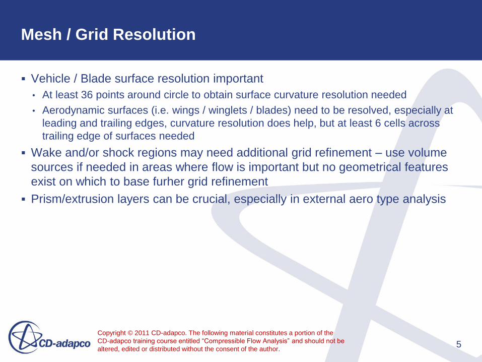
Mesh / Grid Resolution
Vehicle / Blade surface resolution important
• At least 36 points around circle to obtain surface curvature resolution needed
• Aerodynamic surfaces (i.e. wings / winglets / blades) need to be resolved, especially at
leading and trailing edges, curvature resolution does help, but at least 6 cells across
trailing edge of surfaces needed
Wake and/or shock regions may need additional grid refinement – use volume
sources if needed in areas where flow is important but no geometrical features
exist on which to base furher grid refinement
Prism/extrusion layers can be crucial, especially in external aero type analysis

Copyright © 2011 CD-adapco. The following material constitutes a portion of the
CD-adapco training course entitled “Compressible Flow Analysis” and should not be
altered, edited or distributed without the consent of the author. 6
Domain Extent Considerations
External aerodynamic analyses
• Large enough domain aroung object / vehicle
• 10 spans width, 15-20 spans for wake region
All flows, recirculation at boundaries should be avoided, especially with shock
present

Copyright © 2011 CD-adapco. The following material constitutes a portion of the
CD-adapco training course entitled “Compressible Flow Analysis” and should not be
altered, edited or distributed without the consent of the author.
Free Stream Boundary
Typically used as ‚far field„ boundary conditions
for external aerodynamic problems
Specify the flow direction, Mach number, static
pressure, static temperature and turbulence
quantities
• Flow direction may be specified by Flow Angles
(see next slide), Components (in a specified
coordinate system) or as Boundary-Normal
(normal to the boundary surface)
7

Copyright © 2011 CD-adapco. The following material constitutes a portion of the
CD-adapco training course entitled “Compressible Flow Analysis” and should not be
altered, edited or distributed without the consent of the author.
8
Flow Angle Properties
Coordinate System The coordinate system to use.
Cartesian Specifies the Cartesian coordinate system.
Cylindrical Specifies the cylindrical coordinate system.
Laboratory Specifies the laboratory coordinate system.
Spherical Specifies the spherical coordinate system.
Rotation Convention The order in which to apply the rotations specified by the angles.
X Convention (Z-X-Z) For Euler angles (f, q, y), the first rotation is by angle f about the z-axis, the second is by angle q about the x-axis, and
the third is by angle y about the z-axis.
Y Convention (Z-Y-Z) For Euler angles (f, q, y), the first rotation is by angle f about the z-axis, the second is by angle q about the y-axis, and
the third is by angle y about the z-axis.
Yaw, Pitch, Roll Convention (Z-Y-X) For Euler angles (f, q, y ), the first rotation is by angle f about the z-axis, the second is by angle q about the y-axis,
and the third is by angle y about the x-axis.
Axes Convention How to treat the axes during rotations.
Fixed Axes Makes all rotations relative to the original fixed axes.
Moving Axes Makes second and third rotations relative to the rotated axes.
Reference Vector A unit vector that is rotated to convert angles and rotation conventions to a direction. Specified as a single three-part, comma-separated number.
Method Selects the method to use for specifying the angle data.
Constant Specifies the angle as a single three-part, comma-separated number. A Constant node will be added as a child to this
node. For two-dimensional cases, only your entries for the x- and y- directions will be relevant to the calculations
Field Function Defines the angle using a field function (typically user-defined). A Function node will be added as a child to this node
Table (iteration) Defines the angle as a function of iteration number. A Table (iteration) node will be added as a child to this node.
Table (time) Defines the angle as a function of physical time. A Table (time) node will be added as a child to this node.
Free Stream Boundary Flow Angles

Copyright © 2011 CD-adapco. The following material constitutes a portion of the
CD-adapco training course entitled “Compressible Flow Analysis” and should not be
altered, edited or distributed without the consent of the author.
Stagnation Inlet Boundary
Stagnation boundaries need special
consideration in supersonic flows. Pressure
ratio analysis needed to get correct inlet
conditions, i.e. Ptot / Pstat = f ( Mach )
Specify the Supersonic Static Pressure, Total
Pressure, Total Temperature and turbulent
quantities
• Note that both the total pressure and supersonic
pressure are relative to the specified reference
pressure
• The supersonic static pressure is designed to
establish incoming flow rate for a stagnation
boundary that is supersonic (otherwise it is
ignored)
• Be aware that if any time the boundary does go
supersonic (even prior to convergence), this value
will be used and the default or poor choice could
lead to divergence
9

Copyright © 2011 CD-adapco. The following material constitutes a portion of the
CD-adapco training course entitled “Compressible Flow Analysis” and should not be
altered, edited or distributed without the consent of the author.
Mass Flow Inlet Boundary
Most often used in conjunction with pressure
outlets
Specify the flow direction, mass flow rate,
supersonic static pressure, total temperature
and turbulence quantities
• Flow direction options are the same as for free
stream boundaries
• Supersonic static pressure is used only where the
inlet flow us supersonic (as with stagnation inlet
boundaries)
• Mass flow rate may be negative (outflow) despite
the name (see help for additional guidelines on this
option)
10

Copyright © 2011 CD-adapco. The following material constitutes a portion of the
CD-adapco training course entitled “Compressible Flow Analysis” and should not be
altered, edited or distributed without the consent of the author.
Pressure Outlet Boundary
Most often used in conjunction with stagnation
inlet and mass flow inlet boundaries
Specify the pressure, static temperature and
turbulence quantities
• For subsonic outflow, the specified pressure is
applied as a static pressure, while for supersonic
outflow the boundary pressure is extrapolated from
the cell adjacent to the boundary
• Where inflow occurs, the specified pressure is
applied as a total pressure
• Boundary velocities are extrapolated from the
interior in all cases
11

Copyright © 2011 CD-adapco. The following material constitutes a portion of the
CD-adapco training course entitled “Compressible Flow Analysis” and should not be
altered, edited or distributed without the consent of the author.
Initial Conditions
Specify (static) pressure, static temperature,
velocity and turbulence quantities
Intializing pressure:
• If there are no pressure boundaries, the specified
initial pressure must not result in a non-physical
absolute pressure
• For free-stream flows, the initial pressure should
equal the free-stream pressure
• For internal (duct) flows, the initial pressure should
be chosen so that it is equal to or higher than the
outlet pressure (helps to inhibit reversed flow at the
outlet)
It is a good idea to intialize the flow field prior to
running and judge if it makes sense
12

Copyright © 2011 CD-adapco. The following material constitutes a portion of the
CD-adapco training course entitled “Compressible Flow Analysis” and should not be
altered, edited or distributed without the consent of the author. 13
Solver Controls
The Coupled Implicit Solver is strongly recommended for all compressible flows
(especially if Mach number is greater than ~0.3)
For steady flows, the Courant Number is the key control parameter
• Default of 5.0 may be too high, especially for flows with shocks (lower this values to 1.0
or 2.0 and then ramp up over a few hundred iterations)
For transient flows the choice of the time step is crucial
• Set the time step such that the convective Courant number is ~1 everywhere
• Set stopping criteria based on residual tolerances of key variables (especially continuity,
momentum and temperature)
• Set sufficient number of inner iterations for all variables to converge (but not so many
that the solution is inefficient)

Copyright © 2011 CD-adapco. The following material constitutes a portion of the
CD-adapco training course entitled “Compressible Flow Analysis” and should not be
altered, edited or distributed without the consent of the author.
Coupled Flow Model
Advantages of the AUSM+ scheme
• Algorithmic simplicity and straightforward
extension for complex conservation laws
• Accurate capture of shock- and contact-
discontinuity
• Numerical solutions that preserve positivity and
satisfy entropy
• Reduced susceptibility to „carbuncle“ phenomena
AUSM+ recommmended for all compressible
flows
Explicit relaxation offers another way to relax
coupled flow solution (alternative to Courant
number)
• Change the Explicit Relaxation Factor from its
default value (1.0) to a lower value, e.g. 0.25
14

Copyright © 2011 CD-adapco. The following material constitutes a portion of the
CD-adapco training course entitled “Compressible Flow Analysis” and should not be
altered, edited or distributed without the consent of the author.
AMG Solver Controls
If instability persists, then modify
AMG Linear Solver settings
• Increase Convergence Tolerance to 0.1
(from default of 0.01)
• Increase V Cycle > Post-Sweeps to 3
(from default of 1)
• Decrease V Cycle > Max Levels to 2
(from default of 50)
15

Copyright © 2011 CD-adapco. The following material constitutes a portion of the
CD-adapco training course entitled “Compressible Flow Analysis” and should not be
altered, edited or distributed without the consent of the author.
Directional Mesh Reordering
Directional reordering may improve
solution convergence
• Reorder the mesh in the primary flow
direction
• Optimizes solver performance due to
the way it updates solution variables
• Also reduces the „bandwidth“of the
solution, making the solver more
efficient
• Right-click on Regions > [Regions
name] > Reorder Mesh
• In the popup window check the Use
directional reordering box and set the
direction vector as desired
16

Copyright © 2011 CD-adapco. The following material constitutes a portion of the
CD-adapco training course entitled “Compressible Flow Analysis” and should not be
altered, edited or distributed without the consent of the author. 17
Turbulence Modeling
General recommendations
• k-e are the models of choice for internal flows
• Spalart-Allmaras models are often the best choice for external flows with mild or no
separation
• k-w models are a good alternative to Spalart-Allmaras for external flows, especially
those with more severe separation
• Reynolds„ StressTransport models are recommended for flows with anisotropic
turbulence
The All-y+ wall treatment is recommended for any model for which it is available

Copyright © 2011 CD-adapco. The following material constitutes a portion of the
CD-adapco training course entitled “Compressible Flow Analysis” and should not be
altered, edited or distributed without the consent of the author. 18
Esitmation of Desired Near-Wall Cell Size
We generally wish to target a specific value of y+ for the near-wall mesh, where
𝑦+ =𝑢∗𝑦
𝜈 𝑢∗ =
𝜏𝑤𝜌
The wall sheat stress 𝜏𝑤 can be related to the skin friction coefficient:
𝐶𝑓 =𝜏𝑤
𝜌𝑈2
2
The skin friction coefficient can be estimated from correlations
• For a flat plate
• For pipe flow
𝐶𝑓
2=
0.036
𝑅𝑒𝐿1 5
𝐶𝑓
2=
0.039
𝑅𝑒𝐷1 5

Copyright © 2011 CD-adapco. The following material constitutes a portion of the
CD-adapco training course entitled “Compressible Flow Analysis” and should not be
altered, edited or distributed without the consent of the author. 19
Judging Convergence
For steady state, is solution unchanging?
• Do shock locations remain constant?
• Do vortices/separation points/recirculation zones remain unchanging over a number of
iterations?
• Constant temperature and pressure fields?
For transients, is each time step converging to the prescribed inner iterations
convergence criterion before reaching the maximum number of inner iterations?
Key data monitor settle to a constant value
• External aero lift/drag forces or Cl/Cd coefficients level off at a constant value
• Flow rates settle to constant values (such as in turbomachinery cases)
• Any other engineering quantities of note (swirl, forces, moments, etc.) are monitored
throughout and settle to constant values

Copyright © 2011 CD-adapco. The following material constitutes a portion of the
CD-adapco training course entitled “Compressible Flow Analysis” and should not be
altered, edited or distributed without the consent of the author. 20
Nozzle Best Practices
Set initial conditions to have pressure and temperature values as they would be
at Mach = 0.8
• This will help provide an initial velocity in the flow direction that is somewhat
representative and enables the flow to „wash“ over the geometry
• Without doing so, there is risk of low pressure „vacuum“ regions occuring which could
lead to instabilities
If convergence issues related to turbulence arise, try raising the turbulence
intensity to 0.1 and the turbulent viscosity ratio to 1000 for the initial and inflow
boundary conditions
At startup, a lot can happen and the vast gradients between a near laminar
startup and a turbulent flow early on could prove problematic for the solver
If the values for turbulence happen to be known at the boundaries, use these if
they are reasonable

Copyright © 2011 CD-adapco. The following material constitutes a portion of the
CD-adapco training course entitled “Compressible Flow Analysis” and should not be
altered, edited or distributed without the consent of the author. 21
Nozzle Best Practices
KEY POINT: Ramp down exit pressure boundary conditions for temperature and
pressure using field functions

Copyright © 2011 CD-adapco. The following material constitutes a portion of the
CD-adapco training course entitled “Compressible Flow Analysis” and should not be
altered, edited or distributed without the consent of the author. 22
Nozzle Best Practices
Results!
Note: The black and white d(rho)/d(P) result is obtained by
turning on temporary storage for the coupled solver settings)

Copyright © 2011 CD-adapco. The following material constitutes a portion of the
CD-adapco training course entitled “Compressible Flow Analysis” and should not be
altered, edited or distributed without the consent of the author. 23
Analysis Output/Post Processing
Contour Plots of
• Temperature
• Pressure
• Density
• Mach Number
• Velocity Magnitude
- All these help examine the physical nature of the flow and if there are shocks, are great properties
to visualize them!
- Can also help judge convergence of the flow fields
Velocity vector plots (to examine flow direction, swirl, wake, vortices, etc.)
Reports
• Lift/Drag monitors and plots for forces and coefficients are almost assuredly needed to
judge convergence and report results for external aero cases

Copyright © 2011 CD-adapco. The following material constitutes a portion of the
CD-adapco training course entitled “Compressible Flow Analysis” and should not be
altered, edited or distributed without the consent of the author. 24
Heat Transfer Coefficients & Adiabatic Wall Temperature
For external high-speed (compressible) flows, the appropriate choice of fluid
temperature is the „adiabatic wall temperature“
• An adjustment to the freestream temperature, it accounts for compressibility and viscous
dissipation effects
Adiabatic wall temperature is defined as:
𝑇𝑎𝑤 = 𝑇∞ 1 +1
2𝑟𝑐 𝛾 − 1 𝑀2
where 𝑇∞ is the freestream temperature, g is the specific heat ratio, M is the Mach number
and 𝑟𝑐 is the „recovery factor“
The recovery factor may be approximated by:
𝑟𝑐 ≈ 𝑃𝑟1 2 (laminar flow)
𝑟𝑐 ≈ 𝑃𝑟1 3 (turbulent flow)
Copyright © 2011 CD-adapco. The following material constitutes a portion of the
CD-adapco training course entitled “Compressible Flow Analysis” and should not be
altered, edited or distributed without the consent of the author.
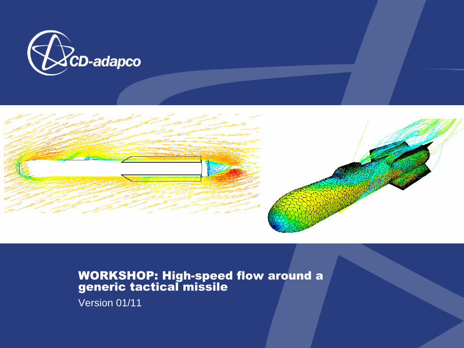
WORKSHOP: High-speed flow around a
generic tactical missile
Version 01/11

Copyright © 2011 CD-adapco. The following material constitutes a portion of the
CD-adapco training course entitled “Compressible Flow Analysis” and should not be
altered, edited or distributed without the consent of the author. 28
Outline
Problem definition
• High-speed flow around a generic tactical missile (subsonic, transonic, supersonic)
• Various angles of attack may be simulated
Key features
• Polyhedral meshing with prismatic layers
• Freestream boundary condition used around the missile
Important boundary numbers
• Mach number: 1.5
• Angle of attack (AOA): 20 deg
• Static temperature: 293 K
• Static presure: 101325 Pa
• Feel free to change the above conditions as desired!

Copyright © 2011 CD-adapco. The following material constitutes a portion of the
CD-adapco training course entitled “Compressible Flow Analysis” and should not be
altered, edited or distributed without the consent of the author.
Data import
Load an existing simulation
• File > Load Simulation... or click on the
load icon in the System toolbar
• Browse to tacmissile_tutorial.sim
• Click Ok
29

Copyright © 2011 CD-adapco. The following material constitutes a portion of the
CD-adapco training course entitled “Compressible Flow Analysis” and should not be
altered, edited or distributed without the consent of the author.
Set Scene Parameters
Open the existing scene
• Right-click Scenes > Geometry Scene 1
> Open
Using the camera icon in the Vis
toolbar select
• Look Down > +X +Y +Z > Up +Y
Make scene transparent
• Click on the transparent icon in the
Vis toolbar
30

Copyright © 2011 CD-adapco. The following material constitutes a portion of the
CD-adapco training course entitled “Compressible Flow Analysis” and should not be
altered, edited or distributed without the consent of the author. 31
Save The Model
It„s a good idea to save the model every time you„ve accomplished a specific set
of tasks and you„re pretty sure that everything is okay with the model
• On the main menu, under File, choose save or simply click on the icon in the System
toolbar

Copyright © 2011 CD-adapco. The following material constitutes a portion of the
CD-adapco training course entitled “Compressible Flow Analysis” and should not be
altered, edited or distributed without the consent of the author.
Check Surface
Check the surface
• Right-click on Geometry > Parts
> tacmissile > Repair Surface...
• Click OK
In the new tab click on Start
Diagnostics, leave all defaults
and click OK
The check reveals that the
surface has 5 Pierced Faces,
1916 Poor Quality Faces and
16 Close Proximity Faces but
no other problems
We will use the Surface
Remesher to improve the
quality of the surface
32
Copyright © 2011 CD-adapco. The following material constitutes a portion of the
CD-adapco training course entitled “Compressible Flow Analysis” and should not be
altered, edited or distributed without the consent of the author.
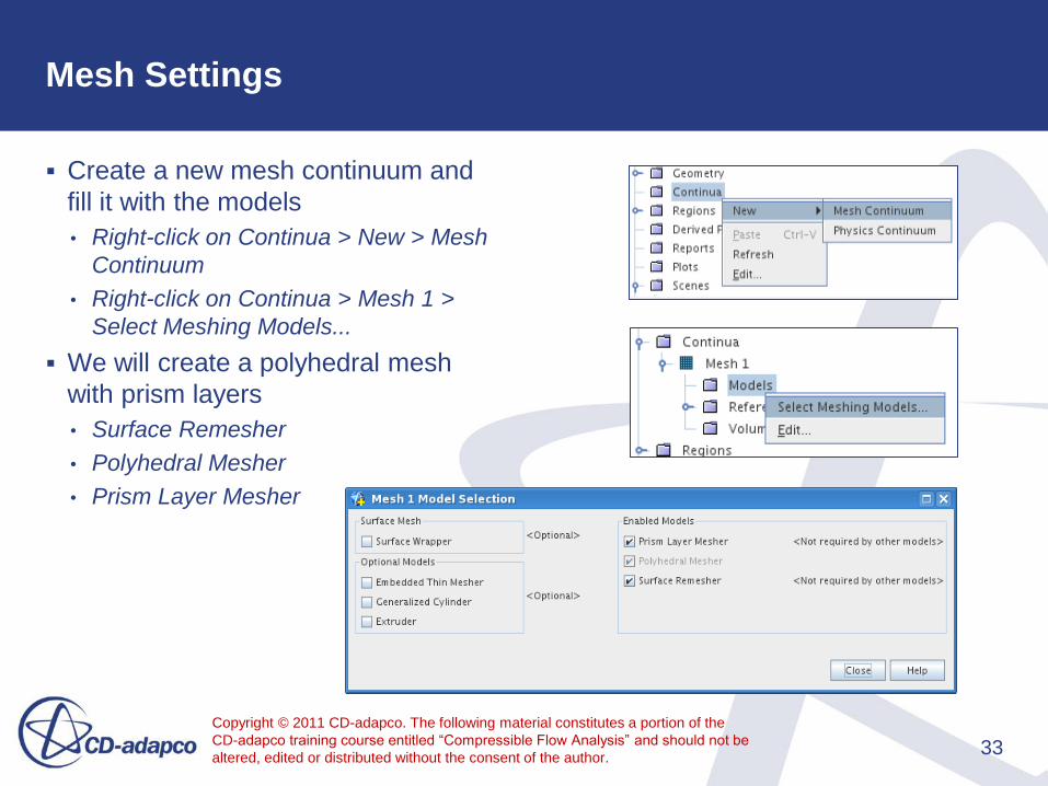
Mesh Settings
Create a new mesh continuum and
fill it with the models
• Right-click on Continua > New > Mesh
Continuum
• Right-click on Continua > Mesh 1 >
Select Meshing Models...
We will create a polyhedral mesh
with prism layers
• Surface Remesher
• Polyhedral Mesher
• Prism Layer Mesher
33

Copyright © 2011 CD-adapco. The following material constitutes a portion of the
CD-adapco training course entitled “Compressible Flow Analysis” and should not be
altered, edited or distributed without the consent of the author.
Mesh Reference Values
Set the reference values, these will be the default
mesh parameters used on all boundaries
• Right-click on Mesh 1 > Reference Values > Edit...
Tet/Poly Density controls the overall volume mesh
density, while the Growth Factor controls the rate of
growth from fine to coarse areas
Tet/Poly Volume Blending controls the rate of cell
growth from volume sources
34
Reference Values Value
Base Size 0.2 m
Prism Layer Thickness Relative 2%
Surface Size: Relative Minimum Size
Relative Target Size
2%
20%
Tet/Poly Density Density
Growth Factor
0.6
1.4
Tet/Poly Volume
Blending
Blending Factor 0.8

Copyright © 2011 CD-adapco. The following material constitutes a portion of the
CD-adapco training course entitled “Compressible Flow Analysis” and should not be
altered, edited or distributed without the consent of the author.
Boundary Mesh Values
We will change the default mesh settings at
several boundaries:
The leading edges of the fins requires a
much finer mesh than the rest of the
domain
• Right-click on Regions > Body 1 > Boundaries
> fin LE > Edit...
• Set the values according to the table
Repeat this for fin TE
35
Mesh Conditions fin LE fin TE
Custom Surface Size Yes Yes
Mesh Values
Surface Size: Relative Minimum Size 0.05% 0.5%
Surface Size: Relative Target Size 0.4% 1%

Copyright © 2011 CD-adapco. The following material constitutes a portion of the
CD-adapco training course entitled “Compressible Flow Analysis” and should not be
altered, edited or distributed without the consent of the author.
Boundary Mesh Values
The mesh on the symmetry boundary
needs to be able to grow from a small
size near the missule surface to a
much larger size further away
• Right-click on Regions > Body 1 >
Boundaries > symmetry > Edit...
• Change the boundary type
Boundary Type: Symmetry
• Set the values according to the table
36
Mesh Conditions symmetry
Custom Surface Size Yes
Mesh Values
Surface Size: Relative Minimum Size 1%
Surface Size: Relative Target Size 2000%

Copyright © 2011 CD-adapco. The following material constitutes a portion of the
CD-adapco training course entitled “Compressible Flow Analysis” and should not be
altered, edited or distributed without the consent of the author.
Boundary Mesh Values
The freestream boundary is the
hemisphere sourrounding the one side of
the missile
The mesh here is large, so the Minimum
Surface Size is left at its default while the
Target Surface Size is set to a large value
• Right-click on Regions > Body 1 > Boundaries
> freestream > Edit...
• Change the boundary type
Boundary Type: Free Stream
• Set the values according to the table
37
Mesh Conditions freestream
Custom Surface Size Yes
Mesh Values
Surface Size: Relative Minimum Size 25%
Surface Size: Relative Target Size 2000%

Copyright © 2011 CD-adapco. The following material constitutes a portion of the
CD-adapco training course entitled “Compressible Flow Analysis” and should not be
altered, edited or distributed without the consent of the author.
Volume Mesh Refinement
STAR-CCM+ has the ability to locally
refine the mesh in the region
sourrounded by a volume
• We will do this around the missile
Create the volume
• Right-click on Geometry > Parts > New
Shape Part > Cylinder
• Click Create
38
Start End
X 0 m 0 m
Y 0 m 0 m
Z -0.0224 m 0.1047 m
Radius 0.1 m

Copyright © 2011 CD-adapco. The following material constitutes a portion of the
CD-adapco training course entitled “Compressible Flow Analysis” and should not be
altered, edited or distributed without the consent of the author.
Volume Mesh Refinement
Create a volumetric control with the
cylinder as volume source
• Right-click Contina > Mesh 1 >
Volumetric Control > New
• Right-click Volumetric Control 1 > Edit...
Use the newly created cylinder as
input part
Part Group: Cylinder
• Set the values according to the table
39
Mesh Conditions freestream
Polyhedral Mesher: Customize Yes
Surface Remesher: Customize Yes
Mesh Values
Custom Size: Relative Size 6%

Copyright © 2011 CD-adapco. The following material constitutes a portion of the
CD-adapco training course entitled “Compressible Flow Analysis” and should not be
altered, edited or distributed without the consent of the author.
Physics Settings
Create a new physics continuum and fill it
with the models
• Right-click on Continua > New > Physics
Continuum
• Right-click on Continua > Physics 1 > Select
Models...
For high-speed compressible flow the
coupled solvers are best
We expect significant flow separation at this
large angle of attack, so the SST (Menter)
K-Omega model with All y+ Wall Treatment
is chosen
• Three Dimensional
• Steady
• Gas
• Coupled Flow
40
• Turbulent
• K-Omega Turbulence

Copyright © 2011 CD-adapco. The following material constitutes a portion of the
CD-adapco training course entitled “Compressible Flow Analysis” and should not be
altered, edited or distributed without the consent of the author.
Solver Settings
The AUSM+ FVS scheme is chosen
for the coupled solver
• Physics 1 > Models > Coupled Flow
• Set AUSM+ FVS in the properties
window as the scheme for Coupled
Inviscid Flux
41

Copyright © 2011 CD-adapco. The following material constitutes a portion of the
CD-adapco training course entitled “Compressible Flow Analysis” and should not be
altered, edited or distributed without the consent of the author.
Air Material Properties
Deceleration of the flow near the
missile surface will create large static
temperature gradients, so
Sutherland‘s Law is used for
Dynamic Viscosity and Thermal
Conductivity
• Right-click Physics 1 > Models > Air >
Material Properties > Edit...
• Choose Sutherland‘s Law, leave the
default values
Other properties have a weaker
temperature dependence and are left
constant
42
Copyright © 2011 CD-adapco. The following material constitutes a portion of the
CD-adapco training course entitled “Compressible Flow Analysis” and should not be
altered, edited or distributed without the consent of the author.
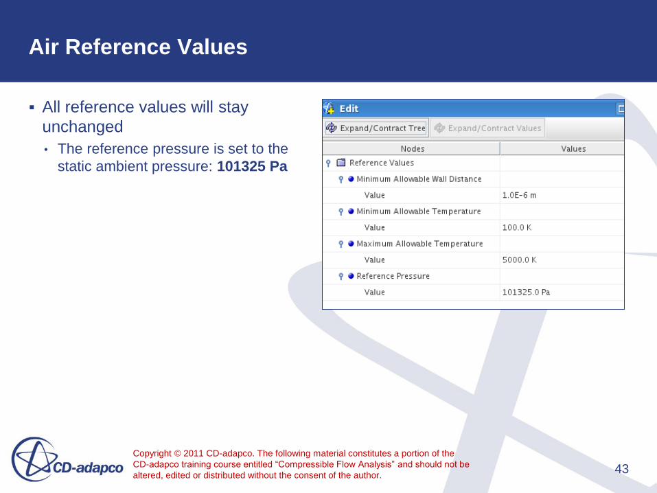
Air Reference Values
All reference values will stay
unchanged
• The reference pressure is set to the
static ambient pressure: 101325 Pa
43

Copyright © 2011 CD-adapco. The following material constitutes a portion of the
CD-adapco training course entitled “Compressible Flow Analysis” and should not be
altered, edited or distributed without the consent of the author.
Air Initial Conditions
The static pressure is relative to the
reference pressure, so it is set to
zero
The static temperature is set to the
ambient temperature
The velocity components correspond
to the specified Mach number,
ambient temperature and angle of
attack
• Right-click on Continua > Physics 1 >
Initial Conditions > Edit...
44
Initial Parameter Value
Velocity Components [0.0, 176.06, 483.72] m/s

Copyright © 2011 CD-adapco. The following material constitutes a portion of the
CD-adapco training course entitled “Compressible Flow Analysis” and should not be
altered, edited or distributed without the consent of the author.
Boundary Condition: Free Stream
The physics conditions for the
freestream boundary needs to be
changed
• Right-click Regions > Body 1 >
Boundaries > freestream > Edit...
45
Physics Conditions freestream
Flow Direction Specification Angles
Physics Values
Flow Angles: Reference Vector [0.0, 0.0, 1.0]
Flow Angles: Constant [0.0, -20.0, 0.0] deg]
Mach Number: Constant 1.5

Copyright © 2011 CD-adapco. The following material constitutes a portion of the
CD-adapco training course entitled “Compressible Flow Analysis” and should not be
altered, edited or distributed without the consent of the author. 46
Boundary Conditions
The symmetry boundary is already if type Symmetry Plane
• No other settings are needed for this type of boundary
All other boundaries are adiabatic, no-slip walls which is the default type Wall
Summary of boundary types Boundary Name Boundary Type
freestream Free Stream
symmetry Symmetry Plane
aft
Wall
base
body mid
fin LE
fin sides
fin TE
nose
scoop

Copyright © 2011 CD-adapco. The following material constitutes a portion of the
CD-adapco training course entitled “Compressible Flow Analysis” and should not be
altered, edited or distributed without the consent of the author. 47
Mesh Generation
We are now ready to generate the mesh!!!
We will generate the surface mesh and the volume mesh in two separate steps
• Generate the surface mesh
• See that is it generated successfully (no errors)
• Visually inspect it to see if density is as desired
• Only after these steps are complete should volume mesh generation be attempted
Generate the surface mesh now – this can be done in one of two ways
• On the main menu, select Mesh > Generate Surface Mesh
• Click the Generate Surface Mesh icon on the Mesh Generation toolbar
Generate Surface Mesh
Generate Volume Mesh
Copyright © 2011 CD-adapco. The following material constitutes a portion of the
CD-adapco training course entitled “Compressible Flow Analysis” and should not be
altered, edited or distributed without the consent of the author.
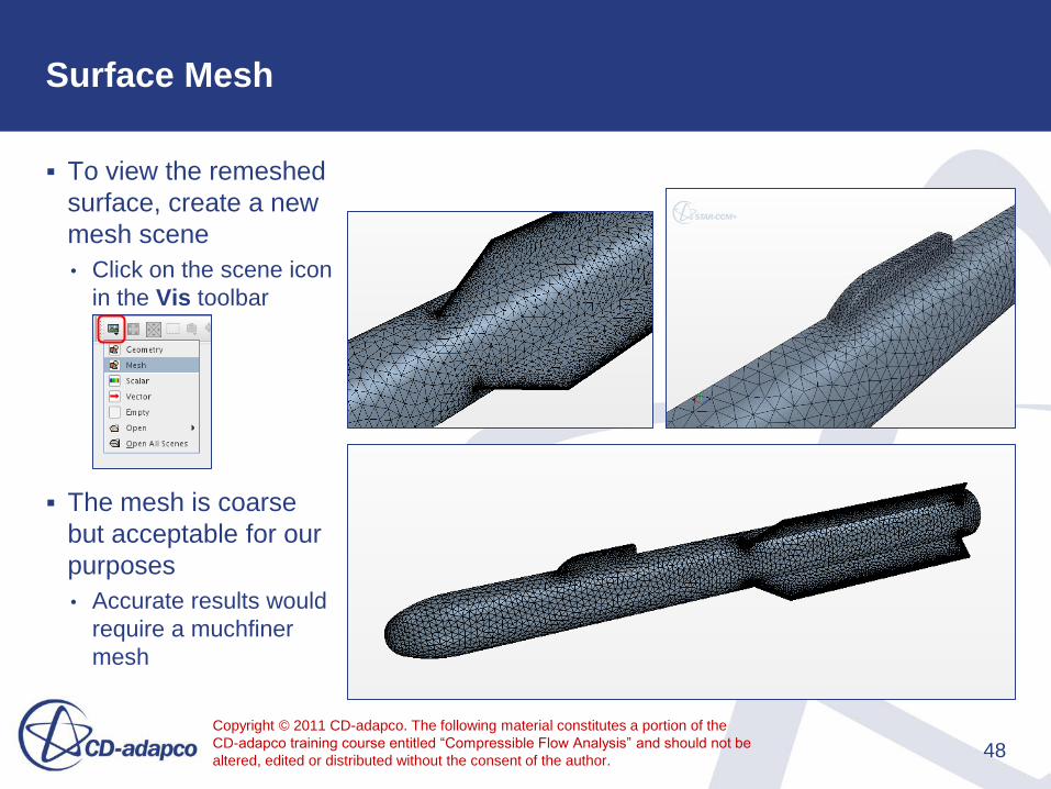
Surface Mesh
To view the remeshed
surface, create a new
mesh scene
• Click on the scene icon
in the Vis toolbar
The mesh is coarse
but acceptable for our
purposes
• Accurate results would
require a muchfiner
mesh
48

Copyright © 2011 CD-adapco. The following material constitutes a portion of the
CD-adapco training course entitled “Compressible Flow Analysis” and should not be
altered, edited or distributed without the consent of the author.
Volume Mesh
Now generate the volume
mesh – again in one of two
ways
• On the main menu, select Mesh
> Generate Volume Mesh
• Click the Generate Volume
Mesh icon on the Mesh
Generation toolbar
To view the volume
mesh create a new
mesh scene
49

Copyright © 2011 CD-adapco. The following material constitutes a portion of the
CD-adapco training course entitled “Compressible Flow Analysis” and should not be
altered, edited or distributed without the consent of the author.
Volume Mesh Section
Create a cut through the geometry
• Change the view using the camera icon
in the Vis toolbar and select Look Down
> +X > Up +Y
• Click on the Create Plane Section icon
and create the section as shown
• Choose to create a New Geometry
Displayer
In the scene/plot tab disable Mesh 1
displayer
• Right-click Mesh Scene 2 > Displayers
> Mesh 1 > Toggle Visibility
50

Copyright © 2011 CD-adapco. The following material constitutes a portion of the
CD-adapco training course entitled “Compressible Flow Analysis” and should not be
altered, edited or distributed without the consent of the author.
Volume Mesh Section
Turn the mesh display on clicking on
the globe icon in the Vis toolbar
Note that there are two prism layers
adjacent to the wall boundaries
forming the surface of the missile
Note also that there are no prism
layers adjacent to the symmetry and
freestream boundaries
Once again the mesh is too coarse
for accurate results, but acceptable
for our purposes
51
Copyright © 2011 CD-adapco. The following material constitutes a portion of the
CD-adapco training course entitled “Compressible Flow Analysis” and should not be
altered, edited or distributed without the consent of the author.
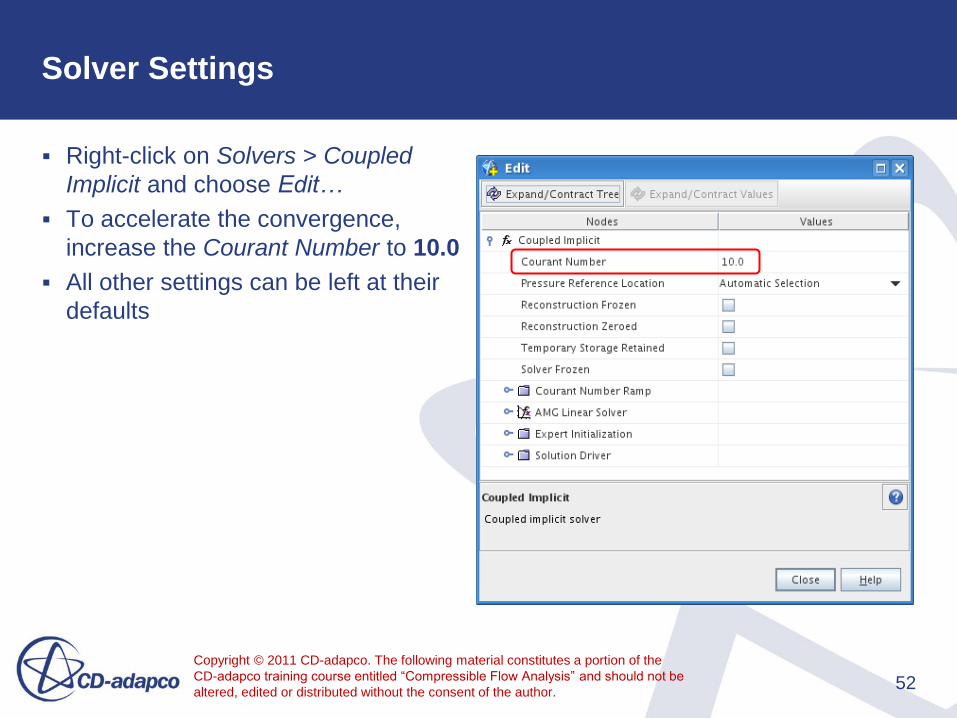
Solver Settings
Right-click on Solvers > Coupled
Implicit and choose Edit…
To accelerate the convergence,
increase the Courant Number to 10.0
All other settings can be left at their
defaults
52

Copyright © 2011 CD-adapco. The following material constitutes a portion of the
CD-adapco training course entitled “Compressible Flow Analysis” and should not be
altered, edited or distributed without the consent of the author.
Stopping Criterion
Click on Stopping Criteria >
Maximum Steps and set the
Maximum Steps to 200
53
Copyright © 2011 CD-adapco. The following material constitutes a portion of the
CD-adapco training course entitled “Compressible Flow Analysis” and should not be
altered, edited or distributed without the consent of the author.
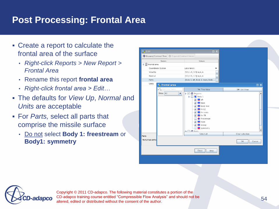
Post Processing: Frontal Area
Create a report to calculate the
frontal area of the surface
• Right-click Reports > New Report >
Frontal Area
• Rename this report frontal area
• Right-click frontal area > Edit…
The defaults for View Up, Normal and
Units are acceptable
For Parts, select all parts that
comprise the missile surface
• Do not select Body 1: freestream or
Body1: symmetry
54
Copyright © 2011 CD-adapco. The following material constitutes a portion of the
CD-adapco training course entitled “Compressible Flow Analysis” and should not be
altered, edited or distributed without the consent of the author. 55
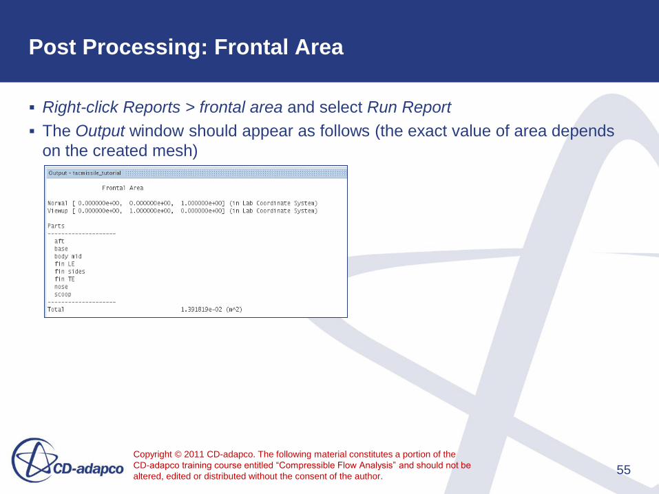
Post Processing: Frontal Area
Right-click Reports > frontal area and select Run Report
The Output window should appear as follows (the exact value of area depends
on the created mesh)
Copyright © 2011 CD-adapco. The following material constitutes a portion of the
CD-adapco training course entitled “Compressible Flow Analysis” and should not be
altered, edited or distributed without the consent of the author.
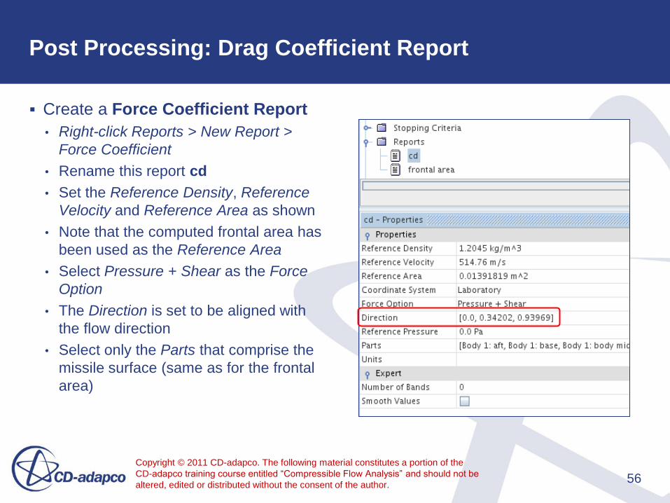
Post Processing: Drag Coefficient Report
Create a Force Coefficient Report
• Right-click Reports > New Report >
Force Coefficient
• Rename this report cd
• Set the Reference Density, Reference
Velocity and Reference Area as shown
• Note that the computed frontal area has
been used as the Reference Area
• Select Pressure + Shear as the Force
Option
• The Direction is set to be aligned with
the flow direction
• Select only the Parts that comprise the
missile surface (same as for the frontal
area)
56

Copyright © 2011 CD-adapco. The following material constitutes a portion of the
CD-adapco training course entitled “Compressible Flow Analysis” and should not be
altered, edited or distributed without the consent of the author.
Post Processing: Lift Coefficient Report
Create a lift coefficient report
The only difference here is the
direction of the force, so we will
simply copy and paste the cd report
and change the direction vector
• Rename the report to cl
57

Copyright © 2011 CD-adapco. The following material constitutes a portion of the
CD-adapco training course entitled “Compressible Flow Analysis” and should not be
altered, edited or distributed without the consent of the author.
Post-Processing: Drag & Lift Coefficient Plots
We must now create monitors and
plots from these reports
• Click on Reports > cd, hold down the
Ctrl key, and click on Reports > cl
While continuing to hold down the
Ctrl key, right click on either report
name and choose Create Monitor
and Plot from Report
In the Create Plot from Reports…
window, select Multiple Plots (one
per report)
58

Copyright © 2011 CD-adapco. The following material constitutes a portion of the
CD-adapco training course entitled “Compressible Flow Analysis” and should not be
altered, edited or distributed without the consent of the author.
Post-Processing: Velocity Vector Scene
Create a new vector scene
• Rename it to Velocity Vectors
• Change the view
- Look Down > +X+Y+Z > Up +Y
Go to the scene/tab panel
• Select Regions > Body 1 > symmetry
to be put in Parts
Click on Displayers > Vector 1 and
change the Vector Scale to Screen
Size in the Properties window
59

Copyright © 2011 CD-adapco. The following material constitutes a portion of the
CD-adapco training course entitled “Compressible Flow Analysis” and should not be
altered, edited or distributed without the consent of the author. 60
Post-Processing: Streamline/Mach Number Scene
We now compose a scene with several displayers, starting with an empty scene
1. Displayer: Scalar displayer showing Mach number on the missile surface
2. Displayer: Streamline displayer
3. Displayer: Geometry displayer showing the mesh on the missile surface

Copyright © 2011 CD-adapco. The following material constitutes a portion of the
CD-adapco training course entitled “Compressible Flow Analysis” and should not be
altered, edited or distributed without the consent of the author.
Post-Processing: Streamline/Mach Number Scene
Create an empty scene
• Rename to Mach Number with Streamlines
• Change the view to Look Down > -X > Up +Y
• We will use a Symmetry Transform for all
displayers, this was automatically created by
STAR-CCM+ using the definition of the
symmetry boundary
61

Copyright © 2011 CD-adapco. The following material constitutes a portion of the
CD-adapco training course entitled “Compressible Flow Analysis” and should not be
altered, edited or distributed without the consent of the author.
Post-Processing: Streamlines
Define new streamlines and add them to a new
displayer in the scene
• Right-click Derived Parts > New Part > Streamline…
• Change the Seed Mode to Line Seed
• Set the starting and ending points for the line seed as
shown, as well as the resolution
• In the Display sub-window, select New Streamline
Displayer
• Click Create
Rename this derived part to streamline
62
Start End
X 0 m -0.04 m
Y -0.9 m -0.09 m
Z -1.5 m -1.5 m
Resolution 40

Copyright © 2011 CD-adapco. The following material constitutes a portion of the
CD-adapco training course entitled “Compressible Flow Analysis” and should not be
altered, edited or distributed without the consent of the author. 63
Post-Processing: Streamline Displayer
In the Scene Explorer of the Mach Number with Streamlines scene, make the
following settings for the streamline displayer:
• Scalar Field: Pressure Coefficient
• Color Bar: invisible
• Transform: symmetry 1

Copyright © 2011 CD-adapco. The following material constitutes a portion of the
CD-adapco training course entitled “Compressible Flow Analysis” and should not be
altered, edited or distributed without the consent of the author.
Post-Processing: Scalar Displayer
Create a new scalar displayer
• Right-click Displayers > New > Scalar
• For Parts, select only the parts that
comprise the missile surface
• As Scalar Field function choose Mach
Number
• Click on the Scalar 1 displayer and in the
properties window change the Contour
Style to Smooth Filled
• Set Transform to symmetry 1
64

Copyright © 2011 CD-adapco. The following material constitutes a portion of the
CD-adapco training course entitled “Compressible Flow Analysis” and should not be
altered, edited or distributed without the consent of the author.
Post-Processing: Geometry Displayer
Create a new scalar displayer
• Right-click Displayers > New > Geometry
• For Parts, select only the parts that
comprise the missile surface
• Click on the Geometry 1 displayer and in
the properties window check the Mesh
box, uncheck the Outline box
• Set Transform to symmetry 1
65

Copyright © 2011 CD-adapco. The following material constitutes a portion of the
CD-adapco training course entitled “Compressible Flow Analysis” and should not be
altered, edited or distributed without the consent of the author. 66
Run Simulation
It‟s now time to run the analysis!!!
This can be done in either of two ways:
• On the main menu, select Solution > Run
• Click the Run button on the Solution toolbar

Copyright © 2011 CD-adapco. The following material constitutes a portion of the
CD-adapco training course entitled “Compressible Flow Analysis” and should not be
altered, edited or distributed without the consent of the author. 67
Residuals Plot

Copyright © 2011 CD-adapco. The following material constitutes a portion of the
CD-adapco training course entitled “Compressible Flow Analysis” and should not be
altered, edited or distributed without the consent of the author. 68
Drag Coefficient Plot
Copyright © 2011 CD-adapco. The following material constitutes a portion of the
CD-adapco training course entitled “Compressible Flow Analysis” and should not be
altered, edited or distributed without the consent of the author. 69
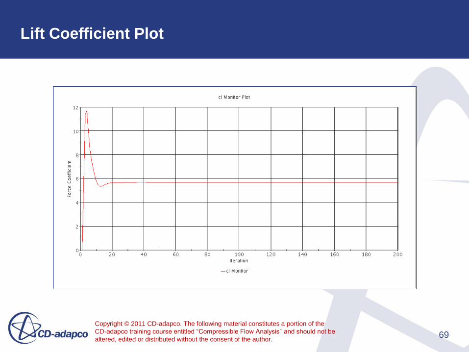
Lift Coefficient Plot

Copyright © 2011 CD-adapco. The following material constitutes a portion of the
CD-adapco training course entitled “Compressible Flow Analysis” and should not be
altered, edited or distributed without the consent of the author. 70
Velocity Vectors Scene

Copyright © 2011 CD-adapco. The following material constitutes a portion of the
CD-adapco training course entitled “Compressible Flow Analysis” and should not be
altered, edited or distributed without the consent of the author. 71
Mach Number with Streamlines Scene

Copyright © 2011 CD-adapco. The following material constitutes a portion of the
CD-adapco training course entitled “Compressible Flow Analysis” and should not be
altered, edited or distributed without the consent of the author. 72
Summary
An analysis of high-speed compressible flow around a missile at 20° AOA has
been performed
A polyhedral mesh with prism layers and local refinement around the fin leading
and trailing edges has been constructed
• It was noted that production analyses should use a much finer mesh than what was
used here
The analysis and post-processing setup was performed

Copyright © 2011 CD-adapco. The following material constitutes a portion of the
CD-adapco training course entitled “Compressible Flow Analysis” and should not be
altered, edited or distributed without the consent of the author.
WORKSHOP: Supersonic Flow in a
Converging-Diverging Nozzle
Version 01/11

Copyright © 2011 CD-adapco. The following material constitutes a portion of the
CD-adapco training course entitled “Compressible Flow Analysis” and should not be
altered, edited or distributed without the consent of the author. 74
Outline
Problem definition
• Steady 2D flow in a converging-diverging nozzle with shocks
Key features
• Polyhedral meshing with prismatic layers
• Stagnation inlet and pressure outlet boundaries
• Coupled implicit solver
• Boundary condition ramping using field functions
Copyright © 2011 CD-adapco. The following material constitutes a portion of the
CD-adapco training course entitled “Compressible Flow Analysis” and should not be
altered, edited or distributed without the consent of the author.
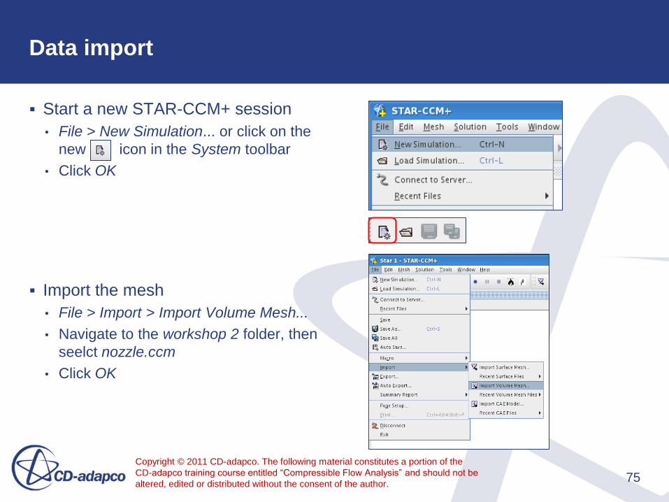
Data import
Start a new STAR-CCM+ session
• File > New Simulation... or click on the
new icon in the System toolbar
• Click OK
Import the mesh
• File > Import > Import Volume Mesh...
• Navigate to the workshop 2 folder, then
seelct nozzle.ccm
• Click OK
75
Copyright © 2011 CD-adapco. The following material constitutes a portion of the
CD-adapco training course entitled “Compressible Flow Analysis” and should not be
altered, edited or distributed without the consent of the author.
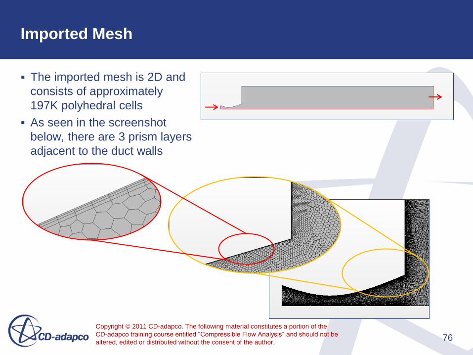
Imported Mesh
The imported mesh is 2D and
consists of approximately
197K polyhedral cells
As seen in the screenshot
below, there are 3 prism layers
adjacent to the duct walls
76

Copyright © 2011 CD-adapco. The following material constitutes a portion of the
CD-adapco training course entitled “Compressible Flow Analysis” and should not be
altered, edited or distributed without the consent of the author.
Physics Settings
Fill the existing physics continuum with models
• Right-click on Continua > Physics 1 > Select
Models...
Note in particular the choice of the
Axisymmetric, Ideal Gas and Coupled solver
models for this analysis (you may need to disable
Two Dimensional)
• Axisymmetric
• Steady
• Gas
• Coupled Flow
• Ideal Gas
• Turbulent
• K-Epsilon Turbulence
77

Copyright © 2011 CD-adapco. The following material constitutes a portion of the
CD-adapco training course entitled “Compressible Flow Analysis” and should not be
altered, edited or distributed without the consent of the author.
Solver Settings
Change the settings of the coupled
flow solver in its properties window
• Continua > Physics 1 > Coupled Flow
- Explicit relaxation: 0.25
- Coupled Inciscid Flux: AUSM+ FVS
78

Copyright © 2011 CD-adapco. The following material constitutes a portion of the
CD-adapco training course entitled “Compressible Flow Analysis” and should not be
altered, edited or distributed without the consent of the author.
Boundary Condition: Axis
Check that the boundary type for axis
boundaries is set to Axis
• With the Ctrl key pressed, select
Regions > Body_1_2D > Boundaries >
far field axis and nozzle axis and check
in the Properties window that Type is
set to Axis
• The icons in front of the boundaries are
also good indicators for the type of the
boundary
• Summary of boundary types:
79
Boundary Name Boundary Type
pressure outlet Pressure
stagnation inlet Stagnation Inlet
far field axis Axis
nozzle axis
near nozzle vertical wall No-slip Wall
nozzle wall
top slip wall Slip Wall

Copyright © 2011 CD-adapco. The following material constitutes a portion of the
CD-adapco training course entitled “Compressible Flow Analysis” and should not be
altered, edited or distributed without the consent of the author.
Boundary Condition: Wall
Ensure that the Shear Stress
Specification for top slip wall is Slip
• Regions > Body_1_2D > Boundaries >
top slip wall > Physcis Conditions >
Shear Stress Specification: Slip
80
Copyright © 2011 CD-adapco. The following material constitutes a portion of the
CD-adapco training course entitled “Compressible Flow Analysis” and should not be
altered, edited or distributed without the consent of the author.
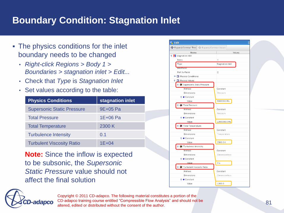
Boundary Condition: Stagnation Inlet
The physics conditions for the inlet
boundary needs to be changed
• Right-click Regions > Body 1 >
Boundaries > stagnation inlet > Edit...
• Check that Type is Stagnation Inlet
• Set values according to the table:
Note: Since the inflow is expected
to be subsonic, the Supersonic
Static Pressure value should not
affect the final solution
81
Physics Conditions stagnation inlet
Supersonic Static Pressure 9E+05 Pa
Total Pressure 1E+06 Pa
Total Temperature 2300 K
Turbulence Intensity 0.1
Turbulent Viscosity Ratio 1E+04
Copyright © 2011 CD-adapco. The following material constitutes a portion of the
CD-adapco training course entitled “Compressible Flow Analysis” and should not be
altered, edited or distributed without the consent of the author.
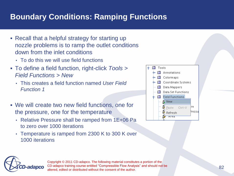
Boundary Conditions: Ramping Functions
Recall that a helpful strategy for starting up
nozzle problems is to ramp the outlet conditions
down from the inlet conditions
• To do this we will use field functions
To define a field function, right-click Tools >
Field Functions > New
• This creates a field function named User Field
Function 1
We will create two new field functions, one for
the pressure, one for the temperature
• Relative Pressure shall be ramped from 1E+06 Pa
to zero over 1000 iterations
• Temperature is ramped from 2300 K to 300 K over
1000 iterations
82

Copyright © 2011 CD-adapco. The following material constitutes a portion of the
CD-adapco training course entitled “Compressible Flow Analysis” and should not be
altered, edited or distributed without the consent of the author. 83
Boundary Conditions: Ramping Functions
Name Function Name Dimensions Definition
P_Down pdown Pressure ($Iteration < 1000) ? 1e6*(1-$Iteration/1000) : 0.0
T_down tdown Temperature ($Iteration < 1000) ? (300 + 2000*(1-$Iteration/1000)) : 300
Copyright © 2011 CD-adapco. The following material constitutes a portion of the
CD-adapco training course entitled “Compressible Flow Analysis” and should not be
altered, edited or distributed without the consent of the author.
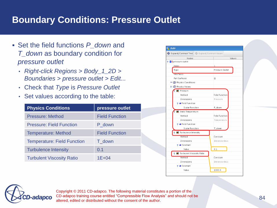
Boundary Conditions: Pressure Outlet
Set the field functions P_down and
T_down as boundary condition for
pressure outlet
• Right-click Regions > Body_1_2D >
Boundaries > pressure outlet > Edit...
• Check that Type is Pressure Outlet
• Set values according to the table:
84
Physics Conditions pressure outlet
Pressure: Method Field Function
Pressure: Field Function P_down
Temperature: Method Field Function
Temperature: Field Function T_down
Turbulence Intensity 0.1
Turbulent Viscosity Ratio 1E+04
Copyright © 2011 CD-adapco. The following material constitutes a portion of the
CD-adapco training course entitled “Compressible Flow Analysis” and should not be
altered, edited or distributed without the consent of the author.
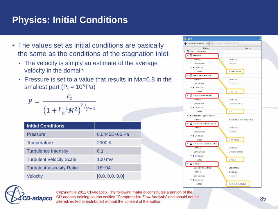
Physics: Initial Conditions
The values set as initial conditions are basically
the same as the conditions of the stagnation inlet
• The velocity is simply an estimate of the average
velocity in the domain
• Pressure is set to a value that results in Ma=0.8 in the
smallest part (Pt = 106 Pa)
85
Initial Conditions
Pressure 6.5445E+05 Pa
Temperature 2300 K
Turbulence Intensity 0.1
Turbulent Velocity Scale 100 m/s
Turbulent Viscosity Ratio 1E+04
Velocity [0.0, 0.0, 0.0]
𝑃 = 𝑃𝑡
1 + 𝛾−12 𝑀2
𝛾𝛾−1
Copyright © 2011 CD-adapco. The following material constitutes a portion of the
CD-adapco training course entitled “Compressible Flow Analysis” and should not be
altered, edited or distributed without the consent of the author.
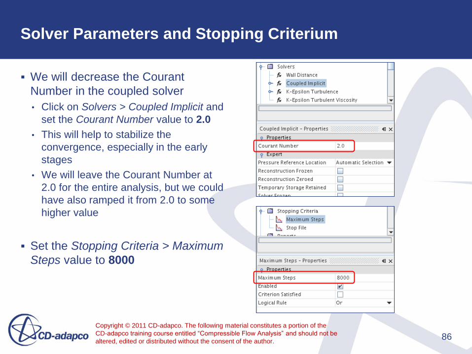
Solver Parameters and Stopping Criterium
We will decrease the Courant
Number in the coupled solver
• Click on Solvers > Coupled Implicit and
set the Courant Number value to 2.0
• This will help to stabilize the
convergence, especially in the early
stages
• We will leave the Courant Number at
2.0 for the entire analysis, but we could
have also ramped it from 2.0 to some
higher value
Set the Stopping Criteria > Maximum
Steps value to 8000
86

Copyright © 2011 CD-adapco. The following material constitutes a portion of the
CD-adapco training course entitled “Compressible Flow Analysis” and should not be
altered, edited or distributed without the consent of the author.
Post Processing: Transform
We will define a transform so that we
can view a serction through the full
3D axisymmetric geometry
• Right-click Tools > Transforms > New
Graphics Transform > Simple
Transform
- This creates a new transform named
Simple Transform 1
• Set the Rotation Angle and Rotation
Axis
87
Transform Properties
Rotation Angle 180 deg
Rotation Axis [1, 0, 0]

Copyright © 2011 CD-adapco. The following material constitutes a portion of the
CD-adapco training course entitled “Compressible Flow Analysis” and should not be
altered, edited or distributed without the consent of the author. 88
Post Processing: Mach Number Scene
We now compose a scene with two scalar displayers
1. Displayer: Scalar displayer showing Mach number
2. Displayer: Scalar displayer, same settings plus Transform
Copyright © 2011 CD-adapco. The following material constitutes a portion of the
CD-adapco training course entitled “Compressible Flow Analysis” and should not be
altered, edited or distributed without the consent of the author.
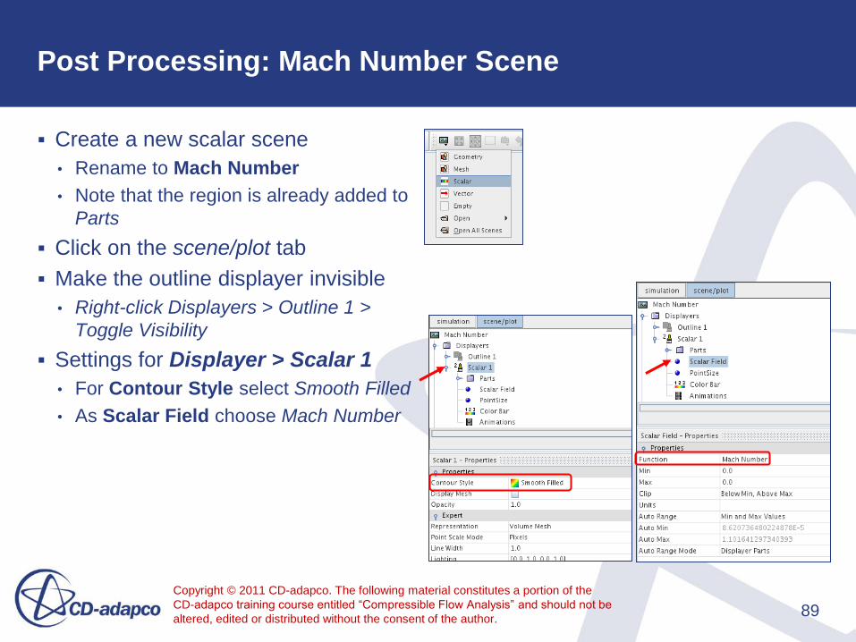
Post Processing: Mach Number Scene
Create a new scalar scene
• Rename to Mach Number
• Note that the region is already added to
Parts
Click on the scene/plot tab
Make the outline displayer invisible
• Right-click Displayers > Outline 1 >
Toggle Visibility
Settings for Displayer > Scalar 1
• For Contour Style select Smooth Filled
• As Scalar Field choose Mach Number
89

Copyright © 2011 CD-adapco. The following material constitutes a portion of the
CD-adapco training course entitled “Compressible Flow Analysis” and should not be
altered, edited or distributed without the consent of the author.
Post Processing: Mach Number Scene
Copy the Scalar 1 displayer
• This creates a new displayer named Copy of Scalar 1
Settings for Displayer > Copy of Scalar 1
• Change Transform to Simple Transform 1
• Uncheck the Visible box under Color Bar
90

Copyright © 2011 CD-adapco. The following material constitutes a portion of the
CD-adapco training course entitled “Compressible Flow Analysis” and should not be
altered, edited or distributed without the consent of the author. 91
Run Simulation
Create other scenes as desired (e.g. for pressure, temperature, velocity vectors)
Now run the simulation in either of two ways:
• On the main menu, select Solution > Run
• Click the Run button on the Solution toolbar
Note: The simulation will run for 8000 iterations for about 3 hours on 4 processors.
To get the following pictures it is necessary to run the simulation much longer.
Increase the Courant number to 5.0 after the first 8000 steps and run it as long as
necessary (approx. 30,000 iterations).

Copyright © 2011 CD-adapco. The following material constitutes a portion of the
CD-adapco training course entitled “Compressible Flow Analysis” and should not be
altered, edited or distributed without the consent of the author.
Mach Number
30,000 iterations
92
8,000 iterations
16,000 iterations

Copyright © 2011 CD-adapco. The following material constitutes a portion of the
CD-adapco training course entitled “Compressible Flow Analysis” and should not be
altered, edited or distributed without the consent of the author.
Absolute Pressure
30,000 iterations
93
8,000 iterations
16,000 iterations

Copyright © 2011 CD-adapco. The following material constitutes a portion of the
CD-adapco training course entitled “Compressible Flow Analysis” and should not be
altered, edited or distributed without the consent of the author.
Temperature
30,000 iterations
94
8,000 iterations
16,000 iterations

Copyright © 2011 CD-adapco. The following material constitutes a portion of the
CD-adapco training course entitled “Compressible Flow Analysis” and should not be
altered, edited or distributed without the consent of the author. 95
Summary
The flow is fairly well-developed and we can see the shock at the nozzle throat
and the beginning of the formation of shock diamonds downstream of the nozzle
It was necessary to reduce the Courant Number for the coupled implicit solver to
2.0 (from the default value of 5.0) to start the solution, but it can probably be
increased now that the important flow features are in place
Field functions were used to ramp down the outlet conditions – this is a useful
approach for many high-speed compressible internal flow problems

Copyright © 2011 CD-adapco. The following material constitutes a portion of the
CD-adapco training course entitled “Compressible Flow Analysis” and should not be
altered, edited or distributed without the consent of the author. 96

Copyright © 2011 CD-adapco
CD-adapco training goes online
For all trainings you attend you get online access to input files and presentation
through the Training Center
Visit https://support.cd-adapco.com to find this material under Past Courses
• Please fill in our online training feedback form that is located there too

STAR-CCM+ User Guide 7361
Version 6.06.015
Transonic Flow over an AirfoilThe tutorial simulates two-dimensional, turbulent, compressible, transonic air flow over an idealized airfoil, as shown below. The free-stream Mach number is 0.725 and the angle of attack is 2.54o. This corresponds to RAE2822 case 6 in Reference [272].
The free-stream flow is subsonic, becoming supersonic on the suction side of the airfoil and subsonic again through a shock wave. The lift and drag coefficients are monitored to help determine whether convergence is reached. The final distribution of the pressure coefficient on the airfoil is then compared to experimental data.
Importing the Mesh and Naming the Simulation
Start up STAR-CCM+ and select the New Simulation option from the menu bar.
Continue by importing the mesh and naming the simulation. A one-cell-thick, three-dimensional, hexahedral mesh has been prepared for this analysis. The mesh corresponds to an angle of attack of 0o in the default Laboratory coordinate system.• Select File > Import > Import Volume Mesh... from the menus.• In the Open dialog, simply navigate to the doc/tutorials/aerofoil
subdirectory of your STAR-CCM+ installation directory and select file aerofoil.ccm which contains the mesh and boundary definitions.
• Click the Open button to start the import.
STAR-CCM+ will provide feedback on the import process, which will take a few seconds, in the Output window. A geometry scene will be created in the Graphics window.
Finally, save the new simulation to disk under file name aerofoil.sim.

STAR-CCM+ User Guide Transonic Flow over an Airfoil 7362
Version 6.06.015
Converting to a Two-Dimensional Mesh
The mesh region can now be converted to a two-dimensional one. There are special requirements in STAR-CCM+ for three-dimensional meshes that need to be converted to two-dimensional. These are: • The grid must be aligned with the X-Y plane.• The grid must have a boundary plane at the Z = 0 location.
The mesh imported for this tutorial was built with these requirements in mind. Were the grid not to conform to the above conditions, it would have been necessary to realign the region using transformation and rotation facilities available in STAR-CCM+.• Select Mesh > Convert to 2D...
• In the Convert Regions to 2D dialog that appears, make sure the checkbox of the Delete 3D regions after conversion option is ticked, and click OK.
Once you have clicked OK, the mesh conversion will take place and the Geometry Scene 1 display will show the two-dimensional geometry in the

STAR-CCM+ User Guide Transonic Flow over an Airfoil 7363
Version 6.06.015
Graphics window. (If the image does not appear immediately, simply click the (Reset View) button on the toolbar.)
All the geometry parts will be shown, viewed from the +z-direction. The mouse rotation option is suppressed for two-dimensional scenes.• Right-click the Physics 1 continuum node and select Delete.• Click Yes in the confirmation dialog.
Setting up the Models
Models define the spatial and temporal solution methods and the physical properties of the flow. In this example, the flow is steady, turbulent and compressible. The default Spalart-Allmaras turbulence model and the ideal gas model will be used. The analysis will also use the coupled solver, which is recommended for all supersonic and transonic compressible flows.
By default, a continuum called Physics 1 2D is created when the mesh is converted to two-dimensional. To use a more appropriate name:• Right-click the Physics 1 2D node and select Rename...Change the name
to Aerofoil.
STAR-CCM+ User Guide Transonic Flow over an Airfoil 7364
Version 6.06.015
The continuum definition will now be edited to select appropriate physical models for the fluid.• Right-click the Aerofoil continuum node and select item Select models.
The Physics Model Selection dialog will guide you through the model selection process by showing only options that are appropriate to the choices already made.• Make sure that the Two Dimensional radio button is selected from the
Space group box.• Select Gas in the Material group box.• Select Coupled Flow in the Flow group box.• Select Ideal Gas in the Equation of State group box.• Select Steady in the Time group box.• Select Turbulent in the Viscous Regime group box.• Select Spalart-Allmaras Turbulence in the Reynolds-Averaged Turbulence
group box.• Click Close.
Inside the Continua node, the color of the Aerofoil node has turned from gray to blue to indicate that models have been activated.• Open the Aerofoil node and then the Models node.
STAR-CCM+ User Guide Transonic Flow over an Airfoil 7365
Version 6.06.015
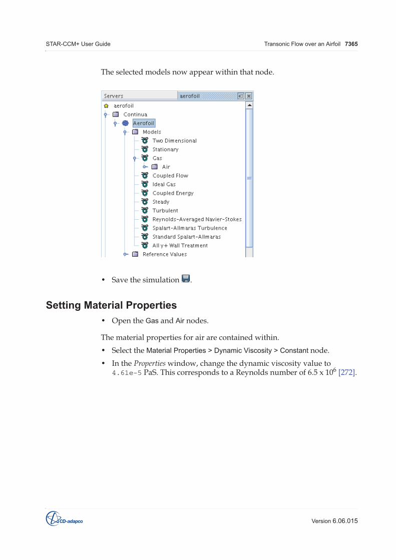
The selected models now appear within that node.
• Save the simulation .
Setting Material Properties• Open the Gas and Air nodes.
The material properties for air are contained within.• Select the Material Properties > Dynamic Viscosity > Constant node.• In the Properties window, change the dynamic viscosity value to
4.61e-5 PaS. This corresponds to a Reynolds number of 6.5 x 10⁶ [272].
STAR-CCM+ User Guide Transonic Flow over an Airfoil 7366
Version 6.06.015
Setting Initial Conditions
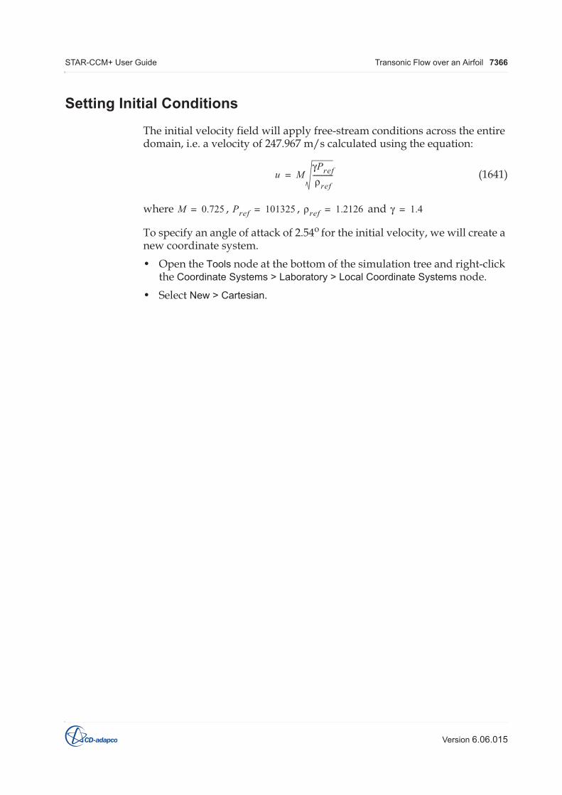
The initial velocity field will apply free-stream conditions across the entire domain, i.e. a velocity of 247.967 m/s calculated using the equation:
(1641)
where , , and
To specify an angle of attack of 2.54o for the initial velocity, we will create a new coordinate system.• Open the Tools node at the bottom of the simulation tree and right-click
the Coordinate Systems > Laboratory > Local Coordinate Systems node.• Select New > Cartesian.
u M�Pref�ref------------=
M 0.725= Pref 101325= �ref 1.2126= � 1.4=

STAR-CCM+ User Guide Transonic Flow over an Airfoil 7367
Version 6.06.015
An in-place dialog will appear to help you create the coordinate system.
• In the Axis Definition group box, change the i Direction to the following:[0.999, 0.0443, 0]
• Click Renormalize. The j Direction will change automatically to ensure that the axes are perpendicular. The i Direction may also readjust itself
STAR-CCM+ User Guide Transonic Flow over an Airfoil 7368
Version 6.06.015
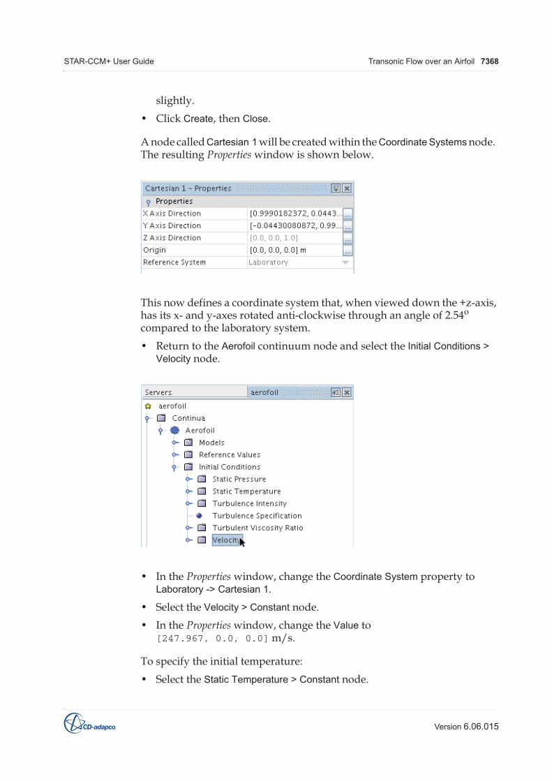
slightly.• Click Create, then Close.
A node called Cartesian 1 will be created within the Coordinate Systems node. The resulting Properties window is shown below.
This now defines a coordinate system that, when viewed down the +z-axis, has its x- and y-axes rotated anti-clockwise through an angle of 2.54o compared to the laboratory system.• Return to the Aerofoil continuum node and select the Initial Conditions >
Velocity node.
• In the Properties window, change the Coordinate System property to Laboratory -> Cartesian 1.
• Select the Velocity > Constant node.• In the Properties window, change the Value to
[247.967, 0.0, 0.0] m/s.
To specify the initial temperature:• Select the Static Temperature > Constant node.
STAR-CCM+ User Guide Transonic Flow over an Airfoil 7369
Version 6.06.015
• In the Properties window change the Value to 291 K.
The default values for the remaining initial conditions are suitable for this problem.
Save the simulation.
Setting Boundary Conditions and Values
The geometry used for this tutorial has only two boundaries:• A wall boundary representing the surface of the airfoil.• A free-stream boundary at the external edge of the solution domain.
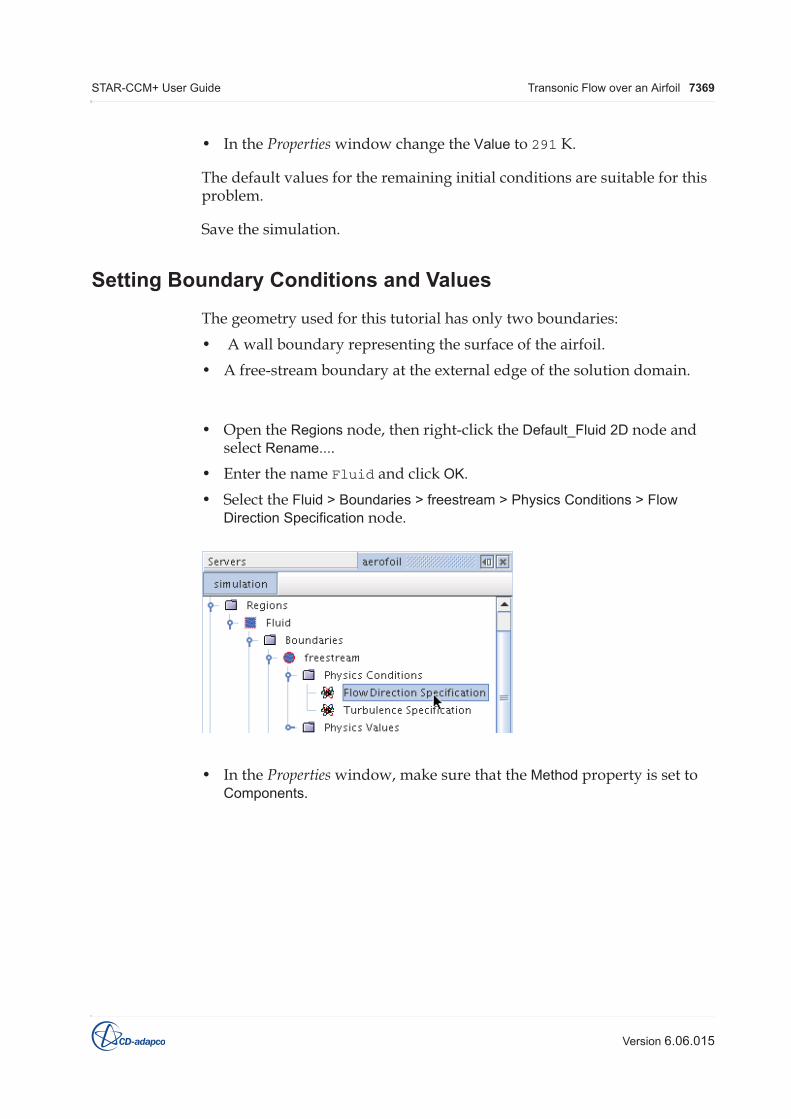
• Open the Regions node, then right-click the Default_Fluid 2D node and select Rename....
• Enter the name Fluid and click OK.• Select the Fluid > Boundaries > freestream > Physics Conditions > Flow
Direction Specification node.
• In the Properties window, make sure that the Method property is set to Components.
STAR-CCM+ User Guide Transonic Flow over an Airfoil 7370
Version 6.06.015
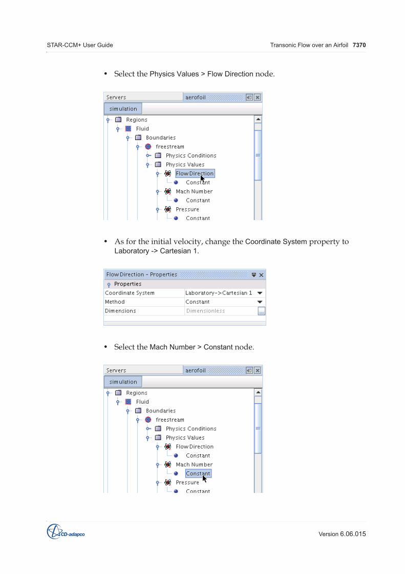
• Select the Physics Values > Flow Direction node.
• As for the initial velocity, change the Coordinate System property to Laboratory -> Cartesian 1.
• Select the Mach Number > Constant node.

STAR-CCM+ User Guide Transonic Flow over an Airfoil 7371
Version 6.06.015
• Change the Value property to 0.725.• Select the Static Temperature > Constant node.• Change the Value property to 291 K.
All other conditions for the free-stream boundary and the default wall boundary conditions are suitable for this problem.
Save the simulation .
Setting Solver Parameters
The simplicity of this problem allows a rapidly converging solution to be attained using a large Courant number. In problems involving more complex geometries or physics, attempting to shorten the run time in this way may cause the run to diverge. To increase the Courant number:• Select the Solvers > Coupled Implicit node.
• In the Properties window, change the Courant Number to 20.0.
Save the simulation.

STAR-CCM+ User Guide Transonic Flow over an Airfoil 7372
Version 6.06.015
Visualizing and Initializing the Solution
We will view the Mach number profile during the run to monitor the supersonic flow region above the airfoil.
Start by creating a new scalar scene.• Right-click on the Scenes node, and select New Scene > Scalar.
The Scalar Scene 1 display will appear.• Right-click on the scalar bar at the bottom of the display and select Mach
Number > Lab Reference Frame from the pop-up menu.
• Initialize the run by clicking the Initialize Solution button in the toolbar, then use the middle mouse button to zoom in on the airfoil in the center

STAR-CCM+ User Guide Transonic Flow over an Airfoil 7373
Version 6.06.015
of the scalar scene.
To change the style of the Mach number contours:• Select the Scalar Scene 1 > Displayers > Scalar 1 node.• In the Properties window, change the Contour Style property to Smooth
Filled.
Save the simulation .
Plotting Graphs
The lift and drag coefficients will be plotted to help in determining when the analysis has converged.

STAR-CCM+ User Guide Transonic Flow over an Airfoil 7374
Version 6.06.015
• Right-click the Reports node and select New Report > Force Coefficient.
A new report node named Force Coefficient 1 will be created.• Rename this node Drag Coefficient then enter the information
shown below in the Properties window.
• Right-click the Drag Coefficient node and select Create Monitor and Plot from Report.
A new plot node will appear named Drag Coefficient Monitor Plot.

STAR-CCM+ User Guide Transonic Flow over an Airfoil 7375
Version 6.06.015
• Double-click on the Drag Coefficient Monitor Plot node to display the empty plot in the Graphics window.
• Repeat the steps described above to create and display a plot for the lift coefficient. All settings should be the same as for the drag coefficient except that the report node should be renamed Lift Coefficient and its Direction property should be set to [-0.0443, 0.9990, 0.0].
Experimental data for the pressure coefficient on the airfoil are provided in file aero_exp.xy in the doc/tutorials/aerofoil directory. These will be plotted on a graph alongside the results of the analysis.
To plot the experimental data:• Right-click the Tools > Tables node and then select New Table > File....• Locate and open file aero_exp.xy• Right-click the Plots node and select New Plot > X-Y.
• Open the XY Plot 1 node, then right-click the Tabular node and select

STAR-CCM+ User Guide Transonic Flow over an Airfoil 7376
Version 6.06.015
New Tabular Data Set.
A new node named tabular will appear within the Tabular node.• In the Properties window, select aero_exp for the Table property.
Make sure that the X Column and Y Column properties are filled as shown below.
A graph of the experimental data will appear in XY Plot 1.
To add the numerical data to the same graph:• Select the XY Plot 1 node.• In the Properties window, click on the Parts property and select Fluid: wall
in the Select Objects dialog.

STAR-CCM+ User Guide Transonic Flow over an Airfoil 7377
Version 6.06.015
• Select the Y Types > Y Type 1 > Scalar node.
• In the Properties window, select Pressure Coefficient for the Scalar property.
The initial pressure coefficient is shown in the XY Plot 1 as being zero everywhere.
The pressure coefficient requires specification of a reference pressure and a reference velocity.• Select the Tools > Field Functions > Pressure Coefficient node.• In the Properties window, enter a Reference Density of 1.2126 kg/m3
and a Reference Velocity of 247.967 m/s, as shown in the following screenshot.

STAR-CCM+ User Guide Transonic Flow over an Airfoil 7378
Version 6.06.015
The usual convention in aerodynamics problems is to reverse the y-axis orientation in pressure coefficient plots.• Select the XY Plot 1 > Axes node.
• Click on the Axis Orientation property and select the option shown below.
The setup is now complete. • Save the simulation .
STAR-CCM+ User Guide Transonic Flow over an Airfoil 7379
Version 6.06.015
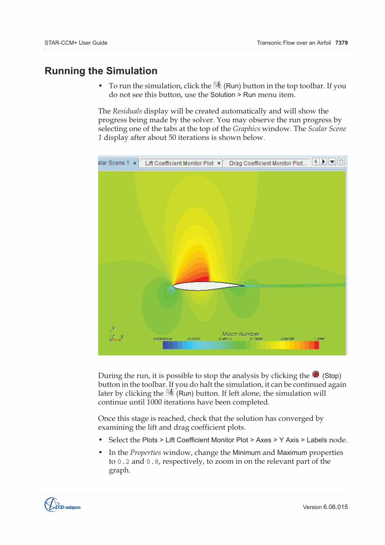
Running the Simulation• To run the simulation, click the (Run) button in the top toolbar. If you
do not see this button, use the Solution > Run menu item.
The Residuals display will be created automatically and will show the progress being made by the solver. You may observe the run progress by selecting one of the tabs at the top of the Graphics window. The Scalar Scene 1 display after about 50 iterations is shown below.
During the run, it is possible to stop the analysis by clicking the (Stop) button in the toolbar. If you do halt the simulation, it can be continued again later by clicking the (Run) button. If left alone, the simulation will continue until 1000 iterations have been completed.
Once this stage is reached, check that the solution has converged by examining the lift and drag coefficient plots.• Select the Plots > Lift Coefficient Monitor Plot > Axes > Y Axis > Labels node.• In the Properties window, change the Minimum and Maximum properties
to 0.2 and 0.8, respectively, to zoom in on the relevant part of the graph.
STAR-CCM+ User Guide Transonic Flow over an Airfoil 7380
Version 6.06.015
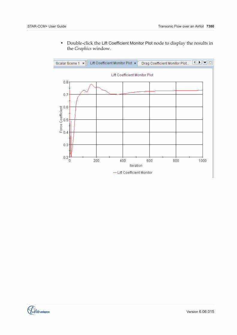
• Double-click the Lift Coefficient Monitor Plot node to display the results in the Graphics window.

STAR-CCM+ User Guide Transonic Flow over an Airfoil 7381
Version 6.06.015
• Similarly, display the drag coefficient plot and adjust its y-axis scale.
Both monitors have reached constant values so it is reasonable to conclude that the solution has converged.• Save the simulation .

STAR-CCM+ User Guide Transonic Flow over an Airfoil 7382
Version 6.06.015
Visualizing the Results
The Scalar Scene 1 display shows the Mach number profile at the end of the run. The profile shows the transonic flow around the airfoil, including the shock wave produced above it.
STAR-CCM+ User Guide Transonic Flow over an Airfoil 7383
Version 6.06.015
Validating the Results
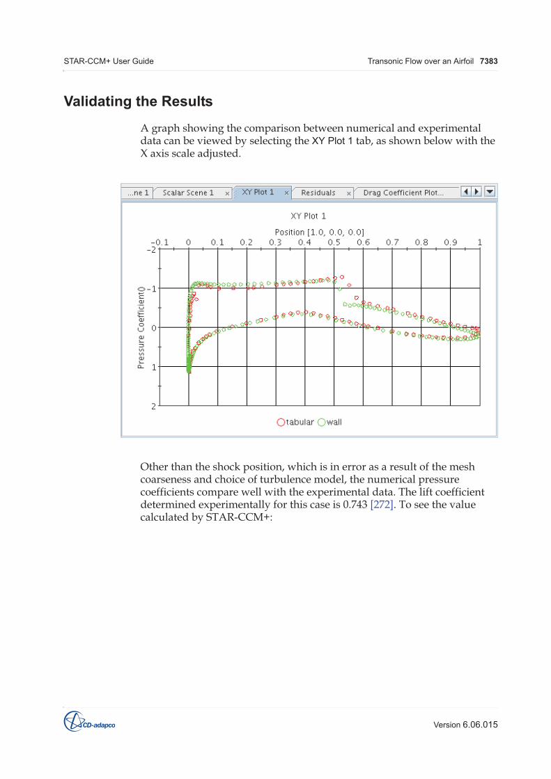
A graph showing the comparison between numerical and experimental data can be viewed by selecting the XY Plot 1 tab, as shown below with the X axis scale adjusted.
Other than the shock position, which is in error as a result of the mesh coarseness and choice of turbulence model, the numerical pressure coefficients compare well with the experimental data. The lift coefficient determined experimentally for this case is 0.743 [272]. To see the value calculated by STAR-CCM+:

STAR-CCM+ User Guide Transonic Flow over an Airfoil 7384
Version 6.06.015
• Right-click the Reports > Lift Coefficient node and then select Run Report.
In the Output window, a tab named Lift Coefficient Report will display the relevant report and show a lift coefficient of 0.732, which is within 2% of the experimental value. Similarly, the drag coefficient report will give a value of 0.0137, which also compares well to the experimental value of 0.0127.
Summary
This STAR-CCM+ tutorial introduced the following features:• Defining models for compressible flow problems.• Defining the material properties required for the selected models.• Setting solver parameters for a steady-state run.• Plotting graphs comparing results with experimental data.• Initializing and running the solver to a specified stopping criterion.• Analyzing the results using the built-in visualization facilities.
Airfoil Tutorial Bibliography[272] Cook, P.H., M.A. McDonald, M.C.P. Firmin “Aerofoil RAE 2822 -
Pressure Distributions, and Boundary Layer and Wake Measurements Experimental Data Base for Computer Program Assessment”, AGARD Report AR 138, 1979