compressible flow - tme085 - chapter 7
TRANSCRIPT

Compressible Flow - TME085
Chapter 7
Niklas Andersson
Chalmers University of Technology
Department of Mechanics and Maritime Sciences
Division of Fluid Mechanics
Gothenburg, Sweden

Chapter 7 - Unsteady Wave Motion

Compressible flow
Basic
Concepts
Com-
pressibility
flow
regimes
speed of
sound
Thermo-
dynamics
thermally
perfect
gas
calorically
perfect
gas
entropy1:st and
2:nd law
High tem-
perature
effects
molecular
motioninternal
energy
Boltzmann
distribution
equilibrium
gas
CFDSpatial
dis-
cretization
Numerical
schemes
Time
integration
Shock
handling
Boundary
conditions
PDE:s
traveling
waves
method
of char-
acteristics
finite
non-linear
waves
acoustic
waves
shock
reflection
moving
shocks
governing
equationsCrocco’s
equation
entropy
equation
substantial
derivativenoncon-
servation
form
conser-
vation
form
Conservation
laws
integral form
Quasi
1D Flowdiffusers
nozzles
governing
equations
2D Flow
shock
expansion
theory
expansion
fansshock
reflection
oblique
shocks
1D Flow
friction
heat
addition
normal
shocks
isentropic
flow
governing
equationsenergy
mo-
mentumcontinuity
Overview

Learning Outcomes
3 Describe typical engineering flow situations in which compressibility effects are
more or less predominant (e.g. Mach number regimes for steady-state flows)
4 Present at least two different formulations of the governing equations for
compressible flows and explain what basic conservation principles they are
based on
8 Derive (marked) and apply (all) of the presented mathematical formulae forclassical gas dynamics
a 1D isentropic flow*
b normal shocks*
j unsteady waves and discontinuities in 1D
k basic acoustics
9 Solve engineering problems involving the above-mentioned phenomena (8a-8k)
11 Explain how the equations for aero-acoustics and classical acoustics are derived
as limiting cases of the compressible flow equations
moving normal shocks - frame of reference seems to be the key here?!Niklas Andersson - Chalmers 4 / 124

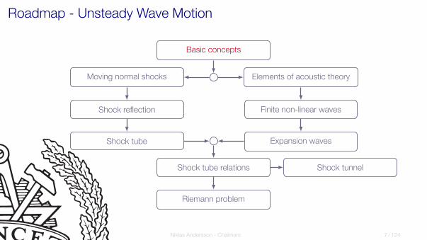
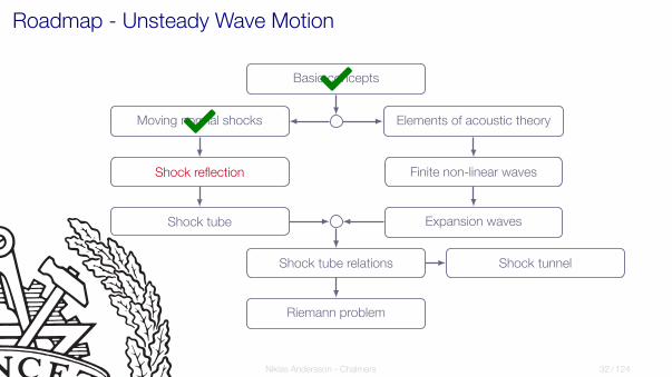
Roadmap - Unsteady Wave Motion
Basic concepts
Moving normal shocks
Shock reflection
Shock tube
Elements of acoustic theory
Finite non-linear waves
Expansion waves
Shock tube relations
Riemann problem
Shock tunnel
Niklas Andersson - Chalmers 5 / 124
Motivation
Most practical flows are unsteady
Traveling waves appears in many real-life situations and is an important topic
within compressible flows
We will study unsteady flows in one dimension in order to reduce complexity
and focus on the physical effects introduced by the unsteadiness
Throughout this section, we will study an application called the shock tube,
which is a rather rare application but it lets us study unsteady waves in one
dimension and it includes all physical principles introduced in chapter 7
Niklas Andersson - Chalmers 6 / 124
Roadmap - Unsteady Wave Motion
Basic concepts
Moving normal shocks
Shock reflection
Shock tube
Elements of acoustic theory
Finite non-linear waves
Expansion waves
Shock tube relations
Riemann problem
Shock tunnel
Niklas Andersson - Chalmers 7 / 124

Unsteady Wave Motion - Example #1
Object moving with supersonic speed through the air
observer moving with the bullet
I steady-state flowI the detached shock wave is
stationary
observer at rest
I unsteady flowI detached shock wave moves
through the air (to the left)
detached shock
Niklas Andersson - Chalmers 8 / 124

Unsteady Wave Motion - Example #1
Object moving with supersonic speed through the air
oblique stationary shock
normal shock advancing
through stagnant air
shock system becomes stationary
only for observer moving with the
object
for stationary observer, both object
and shock system are moving
observermovingwithobject
stationaryobserver
Niklas Andersson - Chalmers 9 / 124

Unsteady Wave Motion - Example #2
Shock wave from explosion
I For observer at rest with respect to the surrounding air:
I the flow is unsteady
I the shock wave moves through the airNiklas Andersson - Chalmers 10 / 124

Unsteady Wave Motion - Example #2
Shock wave from explosion
t = 0.0002 s t = 0.0036 s t = 0.0117 s t = 0.0212 s
t = 0.0308 s t = 0.0404 s t = 0.0499 s t = 0.0594 s
I normal shock moving spherically outwards
I Shock strength decreases with radius
I Shock speed decreases with radius
Niklas Andersson - Chalmers 11 / 124

Unsteady Wave Motion
inertial frames!
Physical laws are the same for both frame of references
Shock characteristics are the same for both observers (shape, strength, etc)
Niklas Andersson - Chalmers 12 / 124

Unsteady Wave Motion
Is there a connection with stationary shock waves?
Answer: Yes!
Locally, in a moving frame of reference, the shock may be viewed as a stationary
normal shock
Niklas Andersson - Chalmers 13 / 124

Roadmap - Unsteady Wave Motion
Basic concepts
Moving normal shocks
Shock reflection
Shock tube
Elements of acoustic theory
Finite non-linear waves
Expansion waves
Shock tube relations
Riemann problem
Shock tunnel
Niklas Andersson - Chalmers 14 / 124

Chapter 7.2
Moving Normal Shock Waves
Niklas Andersson - Chalmers 15 / 124
Moving Normal Shock Waves
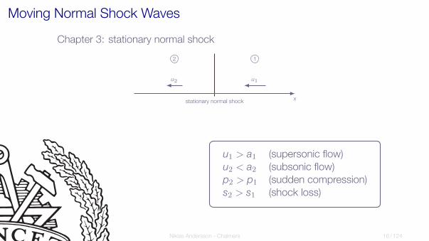
Chapter 3: stationary normal shock
2 1
u2 u1
xstationary normal shock
u1 > a1 (supersonic flow)
u2 < a2 (subsonic flow)
p2 > p1 (sudden compression)
s2 > s1 (shock loss)
Niklas Andersson - Chalmers 16 / 124
Moving Normal Shock Waves
2 1
observerW
u2 u1
xstationary normal shock
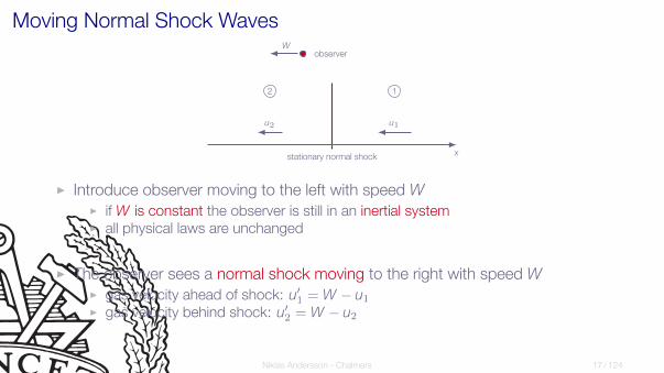
I Introduce observer moving to the left with speed W
I if W is constant the observer is still in an inertial systemI all physical laws are unchanged
I The observer sees a normal shock moving to the right with speed W
I gas velocity ahead of shock: u′1 = W − u1I gas velocity behind shock: u′2 = W − u2
Niklas Andersson - Chalmers 17 / 124

Moving Normal Shock Waves
Now, let W = u1 ⇒
u′1 = 0
u′2 = u1 − u2 > 0
The observer now sees the shock traveling to the right with speed W = u1 into a
stagnant gas, leaving a compressed gas (p2 > p1) with velocity u′2 > 0 behind it
Introducing up:
up = u′2 = u1 − u2
Niklas Andersson - Chalmers 18 / 124

Moving Normal Shock Waves
2 1
stationary observer
u′2 = up > 0 u
′1 = 0
x
W
moving normal shock
Analogy:
Case 1
I stationary normal shockI observer moving with velocity W
Case 2
I normal shock moving with velocity WI stationary observer
Niklas Andersson - Chalmers 19 / 124

Moving Normal Shock Waves - Governing Equations
2 1
stationary observer
u′2 = up > 0 u
′1 = 0
x
W
moving normal shock
For stationary normal shocks we have: With (u1 = W) and (u2 = W − up) weget:
ρ1u1 = ρ2u2
ρ1u21 + p1 = ρ2u
22 + p2
h1 +1
2u21 = h2 +
1
2u22
ρ1W = ρ2(W − up)
ρ1W2 + p1 = ρ2(W − up)
2 + p2
h1 +1
2W2 = h2 +
1
2(W − up)
2
Niklas Andersson - Chalmers 20 / 124

Moving Normal Shock Waves - Relations
Starting from the governing equations
ρ1W = ρ2(W − up)
ρ1W2 + p1 = ρ2(W − up)
2 + p2
h1 +1
2W2 = h2 +
1
2(W − up)
2
and using h = e+p
ρ
it is possible to show that
e2 − e1 =p1 + p2
2
(1
ρ1+
1
ρ2
)Niklas Andersson - Chalmers 21 / 124

Moving Normal Shock Waves - Relations
e2 − e1 =p1 + p2
2
(1
ρ1+
1
ρ2
)
same Hugoniot equation as for stationary normal shock
This means that we will have same shock strength, i.e. same jumps in density,
velocity, pressure, etc
Niklas Andersson - Chalmers 22 / 124

Moving Normal Shock Waves - Relations
Starting from the Hugoniot equation one can show that
ρ2ρ1
=
1 +γ + 1
γ − 1
(p2
p1
)γ + 1
γ − 1+
p2
p1
and
T2
T1=
p2
p1
γ + 1
γ − 1+
p2
p1
1 +γ + 1
γ − 1
(p2
p1
)
Niklas Andersson - Chalmers 23 / 124

Moving Normal Shock Waves - Relations
For calorically perfect gas and stationary normal shock:
p2
p1= 1 +
2γ
γ + 1(M2
s − 1)
same as eq. (3.57) in Anderson with M1 = Ms
where
Ms =W
a1
I Ms is simply the speed of the shock (W ), traveling into the stagnant gas,normalized by the speed of sound in this stagnant gas (a1)
I Ms > 1, otherwise there is no shock!I shocks always moves faster than sound - no warning before it hits you ,
Niklas Andersson - Chalmers 24 / 124

Moving Normal Shock Waves - Relations
5 10 15 201
2
3
4
5
p2/p1
Ms
Incident shock Mach number (γ = 1.4)p2
p1= 1 +
2γ
γ + 1(M2
s − 1)
Re-arrange ⇒
Ms =
√γ + 1
2γ
(p2
p1− 1
)+ 1
shock speed directly linked to pressure ratio
Ms =W
a1⇒ W = a1Ms = a1
√γ + 1
2γ
(p2
p1− 1
)+ 1
Niklas Andersson - Chalmers 25 / 124

Moving Normal Shock Waves - Relations
From the continuity equation we get:
up = W
(1− ρ1
ρ2
)> 0
After some derivation we obtain:
up =a1
γ
(p2
p1− 1
)2γ
γ + 1p2
p1+
γ − 1
γ + 1
1/2
Niklas Andersson - Chalmers 26 / 124

Moving Normal Shock Waves - Relations
Induced Mach number:
Mp =up
a2=
up
a1
a1
a2=
up
a1
√T1
T2
inserting up/a1 and T1/T2 from relations on previous slides we get:
Mp =1
γ
(p2
p1− 1
)2γ
γ + 1γ − 1
γ + 1+
p2
p1
1/2
1 +
(γ + 1
γ − 1
)(p2
p1
)(γ + 1
γ − 1
)(p2
p1
)+
(p2
p1
)2
1/2
Niklas Andersson - Chalmers 27 / 124
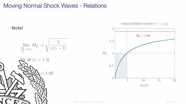
Moving Normal Shock Waves - Relations
Note!
limp2p1
→∞Mp →
√2
γ(γ − 1)
for air (γ = 1.4)
limp2p1
→∞Mp → 1.89
5 10 15 200
0.5
1
1.5
2
Mp = 1.89
p2/p1
Mp
Induced Mach number (γ = 1.4)
Niklas Andersson - Chalmers 28 / 124

Moving Normal Shock Waves - Relations
Moving normal shock with p2/p1 = 10
(p1 = 1.0 bar, T1 = 300 K, γ = 1.4)
⇒ Ms = 2.95 and W = 1024.2 m/s
The shock is advancing with almost three times the speed of sound!
Behind the shock the induced velocity is up = 756.2 m/s ⇒ supersonic flow
(a2 = 562.1 m/s)
May be calculated by formulas 7.13, 7.16, 7.10, 7.11 or by using Table A.2 for stationary normal shock (u1 = W , u2 = W − up )
Niklas Andersson - Chalmers 29 / 124

Moving Normal Shock Waves - Relations
Note! ho1 6= ho2
constant total enthalpy is only valid for stationary shocks!
shock is uniquely defined by pressure ratio p2/p1
u1 = 0
ho1 = h1 +1
2u21 = h1
ho2 = h2 +1
2u22
h2 > h1 ⇒ ho2 > ho1 2 4 6 8 10
1.2
1.4
1.6
1.8
2
p2/p1
γ
h2/h1 = T2/T1 (constant Cp)
1
1.5
2
2.5
3
3.5
4
Niklas Andersson - Chalmers 30 / 124

Moving Normal Shock Waves - Relations
Gas/Vapor Ratio of specific heats Gas constant
(γ) R
Acetylene 1.23 319
Air (standard) 1.40 287
Ammonia 1.31 530
Argon 1.67 208
Benzene 1.12 100
Butane 1.09 143
Carbon Dioxide 1.29 189
Carbon Disulphide 1.21 120
Carbon Monoxide 1.40 297
Chlorine 1.34 120
Ethane 1.19 276
Ethylene 1.24 296
Helium 1.67 2080
Hydrogen 1.41 4120
Hydrogen chloride 1.41 230
Methane 1.30 518
Natural Gas (Methane) 1.27 500
Nitric oxide 1.39 277
Nitrogen 1.40 297
Nitrous oxide 1.27 180
Oxygen 1.40 260
Propane 1.13 189
Steam (water) 1.32 462
Sulphur dioxide 1.29 130
Niklas Andersson - Chalmers 31 / 124
Roadmap - Unsteady Wave Motion
Basic concepts
Moving normal shocks
Shock reflection
Shock tube
Elements of acoustic theory
Finite non-linear waves
Expansion waves
Shock tube relations
Riemann problem
Shock tunnel
Niklas Andersson - Chalmers 32 / 124

Chapter 7.3
Reflected Shock Wave
Niklas Andersson - Chalmers 33 / 124

One-Dimensional Flow with Friction
what happens when a moving shock approaches a wall?
Niklas Andersson - Chalmers 34 / 124
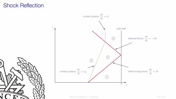
Shock Reflection
x
t
1
5
2
3
initial moving shock,dx
dt= W
reflected shock,dx
dt= −Wr
contact surface,dx
dt= up
contact surface,dx
dt= 0
solid wall
Niklas Andersson - Chalmers 35 / 124

Shock Reflection - Particle Path
A fluid particle located at x0 at time t0 (a location ahead of the shock) will be affected
by the moving shock and follow the blue path
time location velocity
t0 x0 0t1 x0 upt2 x1 upt3 x1 0
x
t
x0 x1t0
t1
t2
t3
Niklas Andersson - Chalmers 36 / 124

Shock Reflection Relations
I velocity ahead of reflected shock: Wr + up
I velocity behind reflected shock: Wr
Continuity:
ρ2(Wr + up) = ρ5Wr
Momentum:
p2 + ρ2(Wr + up)2 = p5 + ρ5W
2r
Energy:
h2 +1
2(Wr + up)
2 = h5 +1
2W2
r
Niklas Andersson - Chalmers 37 / 124

Shock Reflection Relations
Reflected shock is determined such that u5 = 0
Mr
M2r − 1
=Ms
M2s − 1
√1 +
2(γ − 1)
(γ + 1)2(M2
s − 1)
(γ +
1
M2s
)
where
Mr =Wr + up
a2
Niklas Andersson - Chalmers 38 / 124

Tailored v.s. Non-Tailored Shock Reflection
I The time duration of condition 5 is determined by what happens after interaction
between reflected shock and contact discontinuity
I For special choice of initial conditions (tailored case), this interaction is negligible,
thus prolonging the duration of condition 5
Niklas Andersson - Chalmers 39 / 124
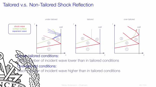
Tailored v.s. Non-Tailored Shock Reflection
5
1
2
3
t
x
wall
under-tailored
5
1
2
3
t
x
wall
tailored
5
1
2
3
t
x
wall
over-tailored
shock wave
contact surface
expansion wave
Under-tailored conditions:
Mach number of incident wave lower than in tailored conditions
Over-tailored conditions:
Mach number of incident wave higher than in tailored conditions
Niklas Andersson - Chalmers 40 / 124

Shock Reflection - Example
Shock reflection in shock tube (γ = 1.4)(Example 7.1 in Anderson)
Incident shock (given data)
p2/p1 10.0
Ms 2.95
T2/T1 2.623
p1 1.0 [bar]
T1 300.0 [K]
Calculated data
Mr 2.09
p5/p2 4.978
T5/T2 1.77
p5 =
(p5
p2
)(p2
p1
)p1 = 49.78
T5 =
(T5
T2
)(T2
T1
)T1 = 1393
Niklas Andersson - Chalmers 41 / 124
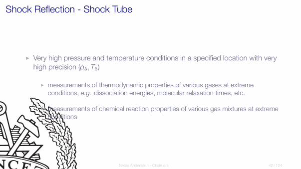
Shock Reflection - Shock Tube
I Very high pressure and temperature conditions in a specified location with very
high precision (p5,T5)
I measurements of thermodynamic properties of various gases at extreme
conditions, e.g. dissociation energies, molecular relaxation times, etc.
I measurements of chemical reaction properties of various gas mixtures at extreme
conditions
Niklas Andersson - Chalmers 42 / 124

Roadmap - Unsteady Wave Motion
Basic concepts
Moving normal shocks
Shock reflection
Shock tube
Elements of acoustic theory
Finite non-linear waves
Expansion waves
Shock tube relations
Riemann problem
Shock tunnel
Niklas Andersson - Chalmers 43 / 124

The Shock Tube
Niklas Andersson - Chalmers 44 / 124

Shock Tube
p
x
p4
p1
4 1
diaphragm
diaphragm location
tube with closed ends
diaphragm inside, separating two differ-
ent constant states
(could also be two different gases)
if diaphragm is removed suddenly (by
inducing a breakdown) the two states
come into contact and a flow develops
assume that p4 > p1:
state 4 is ”driver” section
state 1 is ”driven” section
Niklas Andersson - Chalmers 45 / 124

Shock Tube
t
x
dx
dt= W
dx
dt= up
4
3 2
1
4 3 2 1
Wup
expansion fan contact discontinuity moving normal shock
diaphragm location
flow at some time after diaphragm
breakdown
Niklas Andersson - Chalmers 45 / 124

Shock Tube
p
x
p4
p3 p2
p1
(p3 = p2)
4 3 2 1
Wup
expansion fan contact discontinuity moving normal shock
diaphragm location
flow at some time after diaphragm
breakdown
Niklas Andersson - Chalmers 45 / 124

Shock Tube
I By using light gases for the driver section (e.g. He) and heavier gases for the
driven section (e.g. air) the pressure p4 required for a specific p2/p1 ratio issignificantly reduced
I If T4/T1 is increased, the pressure p4 required for a specific p2/p1 is alsoreduced
Niklas Andersson - Chalmers 46 / 124

Roadmap - Unsteady Wave Motion
Basic concepts
Moving normal shocks
Shock reflection
Shock tube
Elements of acoustic theory
Finite non-linear waves
Expansion waves
Shock tube relations
Riemann problem
Shock tunnel
Niklas Andersson - Chalmers 47 / 124
Chapter 7.5
Elements of Acoustic Theory
Niklas Andersson - Chalmers 48 / 124

Sound Waves
I Weakest audible sound wave (0 dB): ∆p ∼0.00002 PaI Loud sound wave (94 dB): ∆p ∼1 Pa
I Threshold of pain (120 dB): ∆p ∼20 Pa
I Harmful sound wave (130 dB): ∆p ∼60 Pa
Example:
∆p ∼ 1 Pa gives ∆ρ ∼0.000009 kg/m3 and ∆u ∼0.0025 m/s
Niklas Andersson - Chalmers 49 / 124

Sound Waves
Schlieren flow visualization of self-sustained
oscillation of an under-expanded free jet
A. Hirschberg
”Introduction to aero-acoustics of internal flows”,
Advances in Aeroacoustics, VKI, 12-16 March
2001
Intro
ductio
nto
aero
-aco
ustics
ofin
ternalflow
s
A.H
irschberg
Lab
oratoryfor
Flu
idD
ynam
icsFacu
ltyof
Applied
Physics
Tech
nisch
eU
niversiteit
Ein
dhoven
Postb
us
5135600
MB
Ein
dhoven
,N
ederlan
dA
.Hirschb
erg@tu
e.nl
Revised
versionof
chap
terfrom
the
course
Advan
cesin
Aeroacou
stics(V
KI,
12-16M
arch2001)
1.
1Acknow
ledgement:
The
authorw
ishesto
expresshis
gratitudefor
thesupport
ofM
rs.B
.van
deW
ijdevenand
Mr.
D.Tonon
inthe
revisionof
thism
anuscript.T
heflow
visualizationof
jetscreech
hasbeen
providedby
L.Poldervaard
andA
.P.J.W
ijnands.
1
Niklas Andersson - Chalmers 50 / 124

Sound Waves
Screeching rectangular supersonic jet
Niklas Andersson - Chalmers 51 / 124

Elements of Acoustic Theory
PDE:s for conservation of mass and momentum are derived in Chapter 6:
conservation form non-conservation form
mass∂ρ
∂t+ ∇ · (ρv) = 0
Dρ
Dt+ ρ(∇ · v) = 0
momentum∂
∂t(ρv) + ∇ · (ρvv + pI) = 0 ρ
DvDt
+ ∇p = 0
Niklas Andersson - Chalmers 52 / 124

Elements of Acoustic Theory
For adiabatic inviscid flow we also have the entropy equation as
Ds
Dt= 0
Assume one-dimensional flow
ρ = ρ(x, t)v = u(x, t)exp = p(x, t)...
⇒
continuity∂ρ
∂t+ u
∂ρ
∂x+ ρ
∂u
∂x= 0
momentum ρ∂u
∂t+ ρu
∂u
∂x+
∂p
∂x= 0
s=constant
can∂p
∂xbe expressed in terms of density?
Niklas Andersson - Chalmers 53 / 124
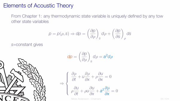
Elements of Acoustic Theory
From Chapter 1: any thermodynamic state variable is uniquely defined by any tow
other state variables
p = p(ρ, s) ⇒ dp =
(∂p
∂ρ
)s
dρ+
(∂p
∂s
)ρ
ds
s=constant gives
dp =
(∂p
∂ρ
)s
dρ = a2dρ
⇒
∂ρ
∂t+ u
∂ρ
∂x+ ρ
∂u
∂x= 0
ρ∂u
∂t+ ρu
∂u
∂x+ a2
∂ρ
∂x= 0
Niklas Andersson - Chalmers 54 / 124

Elements of Acoustic Theory
Assume small perturbations around stagnant reference condition:
ρ = ρ∞ + ∆ρ p = p∞ + ∆p T = T∞ + ∆T u = u∞ + ∆u = {u∞ = 0} = ∆u
where ρ∞, p∞, and T∞ are constant
Now, insert ρ = (ρ∞ +∆ρ) and u = ∆u in the continuity and momentum equations
(derivatives of ρ∞ are zero)
⇒
∂
∂t(∆ρ) + ∆u
∂
∂x(∆ρ) + (ρ∞ + ∆ρ)
∂
∂x(∆u) = 0
(ρ∞ + ∆ρ)∂
∂t(∆u) + (ρ∞ + ∆ρ)∆u
∂
∂x(∆u) + a
2 ∂
∂x(∆ρ) = 0
Niklas Andersson - Chalmers 55 / 124

Elements of Acoustic Theory
Speed of sound is a thermodynamic state variable ⇒ a2 = a2(ρ, s). With entropy
constant ⇒ a2 = a2(ρ)
Taylor expansion around a∞ with (∆ρ = ρ− ρ∞) gives
a2 = a2∞ +
(∂
∂ρ(a2)
)∞∆ρ+
1
2
(∂2
∂ρ2(a2)
)∞(∆ρ)2 + ...
⇒
∂
∂t(∆ρ) + ∆u
∂
∂x(∆ρ) + (ρ∞ + ∆ρ)
∂
∂x(∆u) = 0
(ρ∞ + ∆ρ)∂
∂t(∆u) + (ρ∞ + ∆ρ)∆u
∂
∂x(∆u) +
[a2∞ +
(∂
∂ρ(a
2)
)∞
∆ρ + ...
]∂
∂x(∆ρ) = 0
Niklas Andersson - Chalmers 56 / 124

Elements of Acoustic Theory - Acoustic Equations
Since ∆ρ and ∆u are assumed to be small (∆ρ � ρ∞, ∆u � a)
I products of perturbations can be neglected
I higher-order terms in the Taylor expansion can be neglected
⇒
∂
∂t(∆ρ) + ρ∞
∂
∂x(∆u) = 0
ρ∞∂
∂t(∆u) + a2∞
∂
∂x(∆ρ) = 0
Note! Only valid for small perturbations (sound waves)
This type of derivation is based on linearization, i.e. the acoustic equations are linear
Niklas Andersson - Chalmers 57 / 124
Elements of Acoustic Theory - Acoustic Equations
Acoustic equations:
”... describe the motion of gas induced by the passage of a sound wave ...”
Niklas Andersson - Chalmers 58 / 124
Elements of Acoustic Theory - Wave Equation
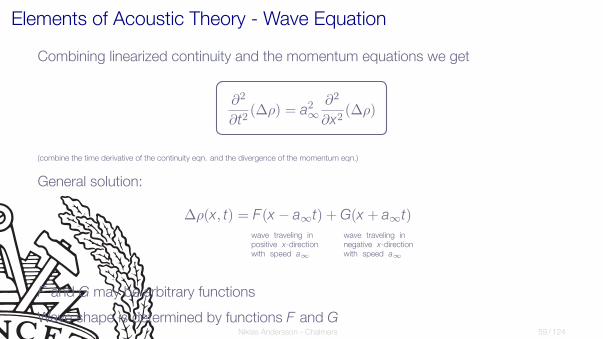
Combining linearized continuity and the momentum equations we get
∂2
∂t2(∆ρ) = a2∞
∂2
∂x2(∆ρ)
(combine the time derivative of the continuity eqn. and the divergence of the momentum eqn.)
General solution:
∆ρ(x, t) = F(x − a∞t) + G(x + a∞t)
wave traveling in
positive x-direction
with speed a∞
wave traveling in
negative x-direction
with speed a∞
F and G may be arbitrary functions
Wave shape is determined by functions F and GNiklas Andersson - Chalmers 59 / 124

Elements of Acoustic Theory - Wave Equation
Spatial and temporal derivatives of F are obtained according to
∂F
∂t=
∂F
∂(x − a∞t)
∂(x − a∞t)
∂t= −a∞F ′
∂F
∂x=
∂F
∂(x − a∞t)
∂(x − a∞t)
∂x= F ′
spatial and temporal derivatives of G can of course be obtained in the same way...
Niklas Andersson - Chalmers 60 / 124

Elements of Acoustic Theory - Wave Equation
with ∆ρ(x, t) = F(x − a∞t) + G(x + a∞t) and the derivatives of F and G we get
∂2
∂t2(∆ρ) = a2∞F ′′ + a2∞G′′
and
∂2
∂x2(∆ρ) = F ′′ +G′′
which gives
∂2
∂t2(∆ρ)− a2∞
∂2
∂x2(∆ρ) = 0
i.e., the proposed solution fulfils the wave equation
Niklas Andersson - Chalmers 61 / 124
Elements of Acoustic Theory - Wave Equation
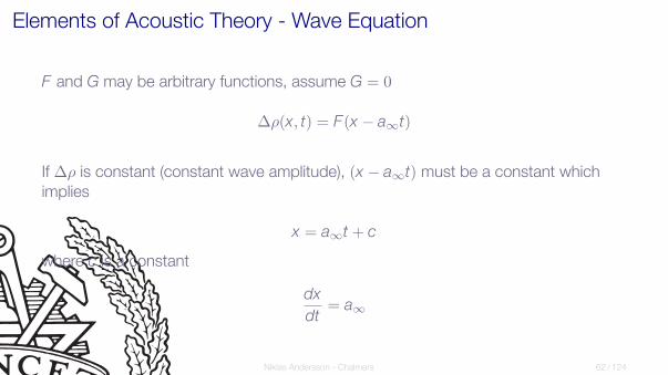
F and G may be arbitrary functions, assume G = 0
∆ρ(x, t) = F(x − a∞t)
If ∆ρ is constant (constant wave amplitude), (x − a∞t) must be a constant whichimplies
x = a∞t + c
where c is a constant
dx
dt= a∞
Niklas Andersson - Chalmers 62 / 124

Elements of Acoustic Theory - Wave Equation
We want a relation between ∆ρ and ∆u
∆ρ(x, t) = F(x − a∞t) (wave in positive x direction) gives:
∂
∂t(∆ρ) = −a∞F ′
and
∂
∂x(∆ρ) = F ′
∂
∂t(∆ρ)︸ ︷︷ ︸
−a∞F ′
+a∞∂
∂x(∆ρ)︸ ︷︷ ︸F ′
= 0
or
∂
∂x(∆ρ) = − 1
a∞
∂
∂t(∆ρ)
Niklas Andersson - Chalmers 63 / 124

Elements of Acoustic Theory - Wave Equation
Linearized momentum equation:
ρ∞∂
∂t(∆u) = −a2∞
∂
∂x(∆ρ) ⇒
∂
∂t(∆u) = −a2∞
ρ∞
∂
∂x(∆ρ) =
{∂
∂x(∆ρ) = − 1
a∞
∂
∂t(∆ρ)
}=
a∞ρ∞
∂
∂t(∆ρ)
∂
∂t
(∆u− a∞
ρ∞∆ρ
)= 0 ⇒ ∆u− a∞
ρ∞∆ρ = const
In undisturbed gas ∆u = ∆ρ = 0 which implies that the constant must be zero andthus
∆u =a∞ρ∞
∆ρ
Niklas Andersson - Chalmers 64 / 124

Elements of Acoustic Theory - Wave Equation
Similarly, for ∆ρ(x, t) = G(x + a∞t) (wave in negative x direction) we obtain:
∆u = −a∞ρ∞
∆ρ
Also, since ∆p = a2∞∆ρ we get:
Right going wave (+x direction) ∆u =a∞ρ∞
∆ρ =1
a∞ρ∞∆p
Left going wave (-x direction) ∆u = −a∞ρ∞
∆ρ = − 1
a∞ρ∞∆p
Niklas Andersson - Chalmers 65 / 124

Elements of Acoustic Theory - Wave Equation
I ∆u denotes induced mass motion and is positive in the positive x-direction
∆u = ±a∞∆ρ
ρ∞= ± ∆p
a∞ρ∞
I condensation (the part of the sound wave where ∆ρ > 0):∆u is always in the same direction as the wave motion
I rarefaction (the part of the sound wave where ∆ρ < 0):∆u is always in the opposite direction as the wave motion
Niklas Andersson - Chalmers 66 / 124

Elements of Acoustic Theory - Wave Equation Summary
Combining linearized continuity and the momentum equations we get
∂2
∂t2(∆ρ) = a2∞
∂2
∂x2(∆ρ)
I Due to the assumptions made, the equation is not exact
I More and more accurate as the perturbations becomes smaller and smaller
I How should we describe waves with larger amplitudes?
Niklas Andersson - Chalmers 67 / 124

Roadmap - Unsteady Wave Motion
Basic concepts
Moving normal shocks
Shock reflection
Shock tube
Elements of acoustic theory
Finite non-linear waves
Expansion waves
Shock tube relations
Riemann problem
Shock tunnel
Niklas Andersson - Chalmers 68 / 124

Chapter 7.6
Finite (Non-Linear) Waves
Niklas Andersson - Chalmers 69 / 124
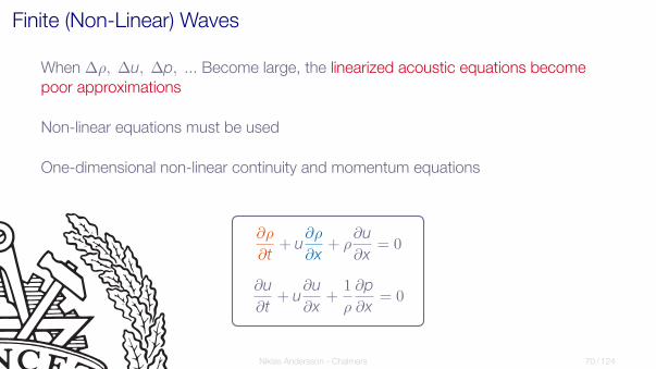
Finite (Non-Linear) Waves
When ∆ρ, ∆u, ∆p, ... Become large, the linearized acoustic equations become
poor approximations
Non-linear equations must be used
One-dimensional non-linear continuity and momentum equations
∂ρ
∂t+ u
∂ρ
∂x+ ρ
∂u
∂x= 0
∂u
∂t+ u
∂u
∂x+
1
ρ
∂p
∂x= 0
Niklas Andersson - Chalmers 70 / 124

Finite (Non-Linear) Waves
We still assume isentropic flow, ds = 0
∂ρ
∂t=
(∂ρ
∂p
)s
∂p
∂t=
1
a2∂p
∂t
∂ρ
∂x=
(∂ρ
∂p
)s
∂p
∂x=
1
a2∂p
∂x
Inserted in the continuity equation this gives:
∂p
∂t+ u
∂p
∂x+ ρa2
∂u
∂x= 0
∂u
∂t+ u
∂u
∂x+
1
ρ
∂p
∂x= 0
Niklas Andersson - Chalmers 71 / 124

Finite (Non-Linear) Waves
Add 1/(ρa) times the continuity equation to the momentum equation:
[∂u
∂t+ (u+ a)
∂u
∂x
]+
1
ρa
[∂p
∂t+ (u+ a)
∂p
∂x
]= 0
If we instead subtraction 1/(ρa) times the continuity equation from the momentum
equation, we get:
[∂u
∂t+ (u− a)
∂u
∂x
]− 1
ρa
[∂p
∂t+ (u− a)
∂p
∂x
]= 0
Niklas Andersson - Chalmers 72 / 124
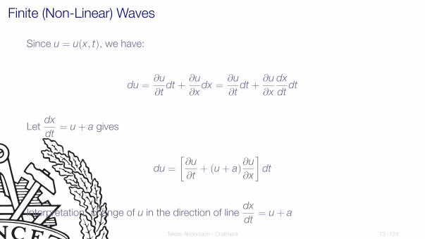
Finite (Non-Linear) Waves
Since u = u(x, t), we have:
du =∂u
∂tdt +
∂u
∂xdx =
∂u
∂tdt +
∂u
∂x
dx
dtdt
Letdx
dt= u+ a gives
du =
[∂u
∂t+ (u+ a)
∂u
∂x
]dt
Interpretation: change of u in the direction of linedx
dt= u+ a
Niklas Andersson - Chalmers 73 / 124

Finite (Non-Linear) Waves
In the same way we get:
dp =∂p
∂tdt +
∂p
∂x
dx
dtdt
and thus
dp =
[∂p
∂t+ (u+ a)
∂p
∂x
]dt
Niklas Andersson - Chalmers 74 / 124

Finite (Non-Linear) Waves
Now, if we combine[∂u
∂t+ (u+ a)
∂u
∂x
]+
1
ρa
[∂p
∂t+ (u+ a)
∂p
∂x
]= 0
du =
[∂u
∂t+ (u+ a)
∂u
∂x
]dt
dp =
[∂p
∂t+ (u+ a)
∂p
∂x
]dt
we get
du
dt+
1
ρa
dp
dt= 0
Niklas Andersson - Chalmers 75 / 124

Characteristic Lines
Thus, along a line dx = (u+ a)dt we have
du+dp
ρa= 0
In the same way we get along a line where dx = (u− a)dt
du− dp
ρa= 0
Niklas Andersson - Chalmers 76 / 124

Characteristic Lines
I We have found a path through a point (x1, t1) along which the governing partialdifferential equations reduces to ordinary differential equations
I These paths or lines are called characteristic lines
I The C+ and C− characteristic lines are physically the paths of right- and
left-running sound waves in the xt-plane
Niklas Andersson - Chalmers 77 / 124

Characteristic Lines
x
t
x1
t1
C−
characteristic line:dx
dt= u − a
compatibility equation: du −dp
ρa= 0
C+
characteristic line:dx
dt= u + a
compatibility equation: du +dp
ρa= 0
Niklas Andersson - Chalmers 78 / 124

Characteristic Lines - Summary
du
dt+
1
ρa
dp
dt= 0 along C+ characteristic
du
dt− 1
ρa
dp
dt= 0 along C− characteristic
du+dp
ρa= 0 along C+ characteristic
du− dp
ρa= 0 along C− characteristic
Niklas Andersson - Chalmers 79 / 124

Riemann Invariants
Integration gives:
J+ = u+
ˆdp
ρa= constant along C+ characteristic
J− = u−ˆ
dp
ρa= constant along C− characteristic
We need to rewritedp
ρato be able to perform the integrations
Niklas Andersson - Chalmers 80 / 124

Riemann Invariants
Let’s consider an isentropic processes:
p = c1Tγ/(γ−1) = c2a
2γ/(γ−1)
where c1 and c2 are constants and thus
dp = c2
(2γ
γ − 1
)a[2γ/(γ−1)−1]da
Assume calorically perfect gas: a2 =γp
ρ⇒ ρ =
γp
a2
with p = c2a2γ/(γ−1) we get ρ = c2γa
[2γ/(γ−1)−2]
Niklas Andersson - Chalmers 81 / 124
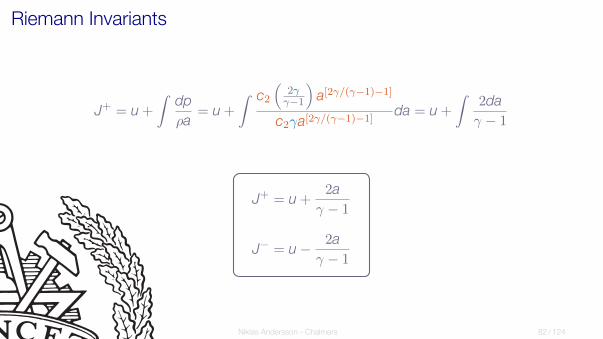
Riemann Invariants
J+ = u+
ˆdp
ρa= u+
ˆ c2
(2γγ−1
)a[2γ/(γ−1)−1]
c2γa[2γ/(γ−1)−1]da = u+
ˆ2da
γ − 1
J+ = u+2a
γ − 1
J− = u− 2a
γ − 1
Niklas Andersson - Chalmers 82 / 124

Riemann Invariants
If J+ and J− are known at some point (x, t), then
J+ + J− = 2u
J+ − J− =4a
γ − 1
⇒
u =
1
2(J+ + J−)
a =γ − 1
4(J+ − J−)
Flow state is uniquely defined!
Niklas Andersson - Chalmers 83 / 124

Method of Characteristics
t
x
tn
tn+1
flow state known
here
flow state may be
computed here
J−
J+
J−
J+
J−
J+
J−
J+
transfer J+
along C+
characteristics, and vice versa
Niklas Andersson - Chalmers 84 / 124

Summary
Acoustic waves
I ∆ρ, ∆u, etc - very small
I All parts of the wave propagate with
the same velocity a∞
I The wave shape stays the same
I The flow is governed by linear
relations
Finite (non-linear) waves
I ∆ρ, ∆u, etc - can be large
I Each local part of the wave
propagates at the local velocity
(u+ a)
I The wave shape changes with time
I The flow is governed by non-linear
relations
Niklas Andersson - Chalmers 85 / 124
One-Dimensional Flow with Friction
the method of characteristics is a central element in classic compressible flow theory
Niklas Andersson - Chalmers 86 / 124

Roadmap - Unsteady Wave Motion
Basic concepts
Moving normal shocks
Shock reflection
Shock tube
Elements of acoustic theory
Finite non-linear waves
Expansion waves
Shock tube relations
Riemann problem
Shock tunnel
Niklas Andersson - Chalmers 87 / 124

Chapter 7.7
Incident and Reflected Expansion
Waves
Niklas Andersson - Chalmers 88 / 124

Expansion Waves
reflected expansion fan
incident shock wave
reflected shock wave
contact surface
1
2
3
4
5
t
x
4 1
driver section driven section
diaphragm location wall
Niklas Andersson - Chalmers 89 / 124

Expansion Waves
Properties of a left-running expansion wave
1. All flow properties are constant along C− characteristics
2. The wave head is propagating into region 4 (high pressure)
3. The wave tail defines the limit of region 3 (lower pressure)
4. Regions 3 and 4 are assumed to be constant states
For calorically perfect gas:
J+ = u+2a
γ − 1is constant along C+ lines
J− = u− 2a
γ − 1is constant along C− lines
Niklas Andersson - Chalmers 90 / 124

Expansion Waves
x
t
C−C−
C−
C−
4
3
Niklas Andersson - Chalmers 91 / 124

Expansion Waves
x
t
C−C−
C−
C−
C+
C+
C+
C+
C+
C+
4
3
Niklas Andersson - Chalmers 91 / 124

Expansion Waves
β
β
β
x
t
a
c
e
b
d
fC−C−
C−
C−
C+
C+
C+
C+
C+
C+
4
3
α α α
constant flow properties in region 4: J+a = J
+b
J+
invariants constant along C+
characteristics:
J+a = J
+c = J
+e
J+b
= J+d
= J+f
since J+a = J
+b
this also implies J+e = J
+f
J−
invariants constant along C−
characteristics:
J−c = J
−d
J−e = J
−f
ue =1
2(J
+e + J
−e ), uf =
1
2(J
+f
+ J−f
), ⇒ ue = uf
ae =γ − 1
4(J
+e − J
−e ), af =
γ − 1
4(J
+f
− J−f
), ⇒ ae = af
Niklas Andersson - Chalmers 91 / 124

Expansion Waves
Along each C− line u and a are constants which means that
dx
dt= u− a = const
C− characteristics are straight lines in xt-space
Niklas Andersson - Chalmers 92 / 124

Expansion Waves
The start and end conditions are the same for all C+ lines
J+ invariants have the same value for all C+ characteristics
C− characteristics are straight lines in xt-space
Simple expansion waves centered at (x, t) = (0, 0)
Niklas Andersson - Chalmers 93 / 124

Expansion Waves
In a left-running expansion fan:
I J+ is constant throughout expansion fan, which implies:
u+2a
γ − 1= u4 +
2a4γ − 1
= u3 +2a3γ − 1
I J− is constant along C− lines, but varies from one line to the next, which means
that
u− 2a
γ − 1
is constant along each C− line
Niklas Andersson - Chalmers 94 / 124

Expansion Waves
Since u4 = 0 we obtain:
u+2a
γ − 1= u4 +
2a4γ − 1
=2a4γ − 1
⇒
a
a4= 1− 1
2(γ − 1)
u
a4
with a =√
γRT we get
T
T4=
[1− 1
2(γ − 1)
u
a4
]2
Niklas Andersson - Chalmers 95 / 124

Expansion Wave Relations
Isentropic flow ⇒ we can use the isentropic relations
complete description in terms of u/a4
T
T4=
[1− 1
2(γ − 1)
u
a4
]2
p
p4=
[1− 1
2(γ − 1)
u
a4
] 2γγ−1
ρ
ρ4=
[1− 1
2(γ − 1)
u
a4
] 2γ−1
Niklas Andersson - Chalmers 96 / 124

Expansion Wave Relations
Since C− characteristics are straight lines, we have:
dx
dt= u− a ⇒ x = (u− a)t
a
a4= 1− 1
2(γ − 1)
u
a4⇒ a = a4 −
1
2(γ − 1)u ⇒
x =
[u− a4 +
1
2(γ − 1)u
]t =
[1
2(γ − 1)u− a4
]t ⇒
u =2
γ + 1
[a4 +
x
t
]Niklas Andersson - Chalmers 97 / 124

Expansion Wave Relations
u
x
u4 = 0
u3
expansion wave
p
x
p4
p3
expansion wave
I Expansion wave head is advancing to the left with
speed a4 into the stagnant gas
I Expansion wave tail is advancing with speed
u3 − a3, which may be positive or negative,
depending on the initial states
Niklas Andersson - Chalmers 98 / 124

Roadmap - Unsteady Wave Motion
Basic concepts
Moving normal shocks
Shock reflection
Shock tube
Elements of acoustic theory
Finite non-linear waves
Expansion waves
Shock tube relations
Riemann problem
Shock tunnel
Niklas Andersson - Chalmers 99 / 124

Chapter 7.8
Shock Tube Relations
Niklas Andersson - Chalmers 100 / 124

Shock Tube Relations
up = u2 =a1
γ
(p2
p1− 1
)2γ1
γ1 + 1p2
p1+
γ1 − 1
γ1 + 1
1/2
p3
p4=
[1− γ4 − 1
2
(u3
a4
)]2γ4/(γ4−1)
solving for u3 gives
u3 =2a4
γ4 − 1
[1−
(p3
p4
)(γ4−1)/(2γ4)]
Niklas Andersson - Chalmers 101 / 124
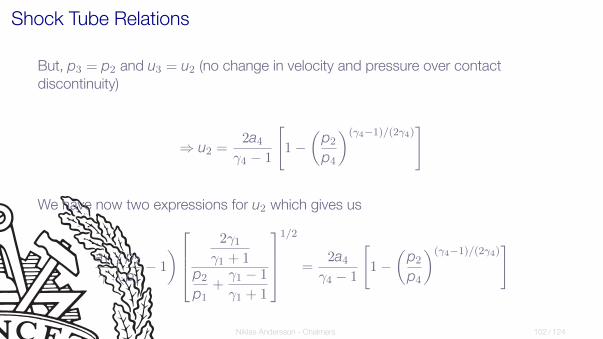
Shock Tube Relations
But, p3 = p2 and u3 = u2 (no change in velocity and pressure over contact
discontinuity)
⇒ u2 =2a4
γ4 − 1
[1−
(p2
p4
)(γ4−1)/(2γ4)]
We have now two expressions for u2 which gives us
a1
γ
(p2
p1− 1
)2γ1
γ1 + 1p2
p1+
γ1 − 1
γ1 + 1
1/2
=2a4
γ4 − 1
[1−
(p2
p4
)(γ4−1)/(2γ4)]
Niklas Andersson - Chalmers 102 / 124

Shock Tube Relations
Rearranging gives:
p4
p1=
p2
p1
{1− (γ4 − 1)(a1/a4)(p2/p1 − 1)√
2γ1 [2γ1 + (γ1 + 1)(p2/p1 − 1)]
}−2γ4/(γ4−1)
I p2/p1 as implicit function of p4/p1
I for a given p4/p1, p2/p1 will increase with decreased a1/a4
a =√
γRT =√γ(Ru/M)T
I the speed of sound in a light gas is higher than in a heavy gas
I driver gas: low molecular weight, high temperatureI driven gas: high molecular weight, low temperature
Niklas Andersson - Chalmers 103 / 124

Roadmap - Unsteady Wave Motion
Basic concepts
Moving normal shocks
Shock reflection
Shock tube
Elements of acoustic theory
Finite non-linear waves
Expansion waves
Shock tube relations
Riemann problem
Shock tunnel
Niklas Andersson - Chalmers 104 / 124

Shock Tunnel
I Addition of a convergent-divergent nozzle to a shock tube configuration
I Capable of producing flow conditions which are close to those during thereentry of a space vehicles into the earth’s atmosphere
I high-enthalpy, hypersonic flows (short time)I real gas effects
I Example - Aachen TH2:
I velocities up to 4 km/sI stagnation temperatures of several thousand degrees
Niklas Andersson - Chalmers 105 / 124

Shock Tunnel
driver section driven section
test section
dump tank
Wr
diaphragm 2diaphragm 1
reflected shock
test object
1. High pressure in region 4 (driver section)I diaphragm 1 burstI primary shock generated
2. Primary shock reaches end of shock tubeI shock reflection
3. High pressure in region 5I diaphragm 2 burstI nozzle flow initiatedI hypersonic flow in test section
Niklas Andersson - Chalmers 106 / 124
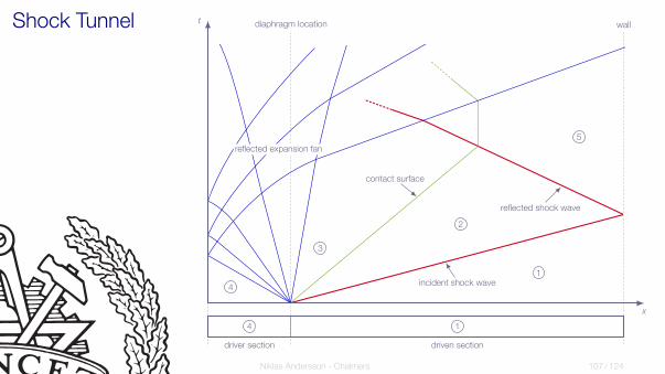
Shock Tunnel
reflected expansion fan
incident shock wave
reflected shock wave
contact surface
1
2
3
4
5
t
x
4 1
driver section driven section
diaphragm location wall
Niklas Andersson - Chalmers 107 / 124
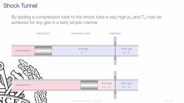
Shock Tunnel
By adding a compression tube to the shock tube a very high p4 and T4 may be
achieved for any gas in a fairly simple manner
heavy piston compression tube diaphragm
pressurized airdriver gas
p, T
driven gas
p1, T1
pressurized airdriver gas
p4, T4
driven gas
p1, T1
Niklas Andersson - Chalmers 108 / 124

The Aachen Shock Tunnel - TH2
Shock tunnel built 1975
nozzle
end of shock tube
inspection window
Niklas Andersson - Chalmers 109 / 124

The Aachen Shock Tunnel - TH2
Shock tube specifications:
diameter 140 mm
driver section 6.0 m
driven section 15.4 m
diaphragm 1 10 mm stainless steel
diaphragm 2 copper/brass sheet
max operating (steady) pressure 1500 bar
Niklas Andersson - Chalmers 110 / 124

The Aachen Shock Tunnel - TH2
I Driver gas (usually helium):
I 100 bar < p4 < 1500 barI electrical preheating (optional) to 600 K
I Driven gas:
I 0.1 bar < p1 < 10 bar
I Dump tank evacuated before test
Niklas Andersson - Chalmers 111 / 124

The Aachen Shock Tunnel - TH2
initial conditions shock reservoir free stream
p4 T4 p1 Ms p2 p5 T5 M∞ T∞ u∞ p∞[bar] [K] [bar] [bar] [bar] [K] [K] [m/s] [mbar]
100 293 1.0 3.3 12 65 1500 7.7 125 1740 7.6
370 500 1.0 4.6 26 175 2500 7.4 250 2350 20.0
720 500 0.7 5.6 50 325 3650 6.8 460 3910 42.0
1200 500 0.6 6.8 50 560 4600 6.5 700 3400 73.0
100 293 0.9 3.4 12 65 1500 11.3 60 1780 0.6
450 500 1.2 4.9 29 225 2700 11.3 120 2480 1.5
1300 520 0.7 6.4 46 630 4600 12.1 220 3560 1.2
26 293 0.2 3.4 12 15 1500 11.4 60 1780 0.1
480 500 0.2 6.6 50 210 4600 11.0 270 3630 0.7
100 293 1.0 3.4 12 65 1500 7.7 130 1750 7.3
370 500 1.0 5.1 27 220 2700 7.3 280 2440 26.3
Niklas Andersson - Chalmers 112 / 124

The Caltech Shock Tunnel - T5
Free-piston shock tunnel
Niklas Andersson - Chalmers 113 / 124

The Caltech Shock Tunnel - T5
I Compression tube (CT):
I length 30 m, diameter 300 mmI free piston (120 kg)I max piston velocity: 300 m/sI driven by compressed air (80 bar - 150 bar)
I Shock tube (ST):
I length 12 m, diameter 90 mmI driver gas: helium + argonI driven gas: airI diaphragm 1: 7 mm stainless steelI p4 max 1300 bar
Niklas Andersson - Chalmers 114 / 124

The Caltech Shock Tunnel - T5
I Reservoir conditions:
I p5 1000 barI T5 10000 K
I Freestream conditions (design conditions):
I M∞ 5.2I T∞ 2000 KI p∞ 0.3 barI typical test time 1 ms
Niklas Andersson - Chalmers 115 / 124

Other Examples of Shock Tunnels
Niklas Andersson - Chalmers 116 / 124
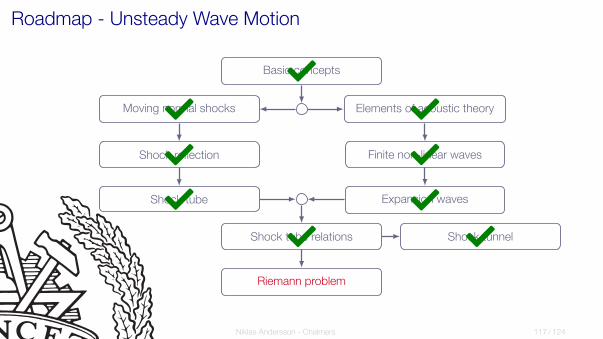
Roadmap - Unsteady Wave Motion
Basic concepts
Moving normal shocks
Shock reflection
Shock tube
Elements of acoustic theory
Finite non-linear waves
Expansion waves
Shock tube relations
Riemann problem
Shock tunnel
Niklas Andersson - Chalmers 117 / 124

Riemann Problem
The shock tube problem is a special case of the general Riemann Problem
”... A Riemann problem, named after Bernhard Riemann, consists of an
initial value problem composed by a conservation equation together with
piecewise constant data having a single discontinuity ...”
Wikipedia
Niklas Andersson - Chalmers 118 / 124

Riemann Problem
May show that solutions to the shock tube problem have the general form:
p = p(x/t)
ρ = ρ(x/t)
u = u(x/t)
T = T(x/t)
a = a(x/t)
where x = 0 denotes the position of theinitial jump between states 1 and 4
Niklas Andersson - Chalmers 119 / 124

Riemann Problem - Shock Tube
Shock tube simulation:
I left side conditions (state 4):I ρ = 2.4 kg/m3
I u = 0.0 m/sI p = 2.0 bar
I right side conditions (state 1):I ρ = 1.2 kg/m3
I u = 0.0 m/sI p = 1.0 bar
I Numerical methodI Finite-Volume Method (FVM) solverI three-stage Runge-Kutta time steppingI third-order characteristic upwinding schemeI local artificial damping
Niklas Andersson - Chalmers 120 / 124

t = 0.0000 s t = 0.0010 s t = 0.0025 s
density
velocity
pressure
0 0.5 1 1.5 2 2.5 3
1.5
2
2.5
0 0.5 1 1.5 2 2.5 3
1.5
2
2.5
0 0.5 1 1.5 2 2.5 3
1.5
2
2.5
0 0.5 1 1.5 2 2.5 3
−0.5
0
0.5
1
0 0.5 1 1.5 2 2.5 3
0
20
40
60
80
100
0 0.5 1 1.5 2 2.5 3
0
20
40
60
80
100
0 0.5 1 1.5 2 2.5 3
1
1.2
1.4
1.6
1.8
2
·105
0 0.5 1 1.5 2 2.5 3
1
1.2
1.4
1.6
1.8
2
·105
0 0.5 1 1.5 2 2.5 3
1
1.2
1.4
1.6
1.8
2
·105

incident shock
contact discontinuity
expansion wave
t = 0.0000 s t = 0.0010 s t = 0.0025 s
density
velocity
pressure
0 0.5 1 1.5 2 2.5 3
1.5
2
2.5
0 0.5 1 1.5 2 2.5 3
1.5
2
2.5
0 0.5 1 1.5 2 2.5 3
1.5
2
2.5
0 0.5 1 1.5 2 2.5 3
−0.5
0
0.5
1
0 0.5 1 1.5 2 2.5 3
0
20
40
60
80
100
0 0.5 1 1.5 2 2.5 3
0
20
40
60
80
100
0 0.5 1 1.5 2 2.5 3
1
1.2
1.4
1.6
1.8
2
·105
0 0.5 1 1.5 2 2.5 3
1
1.2
1.4
1.6
1.8
2
·105
0 0.5 1 1.5 2 2.5 3
1
1.2
1.4
1.6
1.8
2
·105

Riemann Problem - Shock Tube
−1.5 −1 −0.5 0 0.5 1 1.5
1.5
2
2.5
(x/t)× 10−3
ρ
0.0010 s
0.0025 s
−1.5 −1 −0.5 0 0.5 1 1.5
0
20
40
60
80
100
(x/t)× 10−3
u
0.0010 s
0.0025 s
−1.5 −1 −0.5 0 0.5 1 1.5
1
1.2
1.4
1.6
1.8
2
·105
(x/t)× 10−3
p
0.0010 s
0.0025 s
The solution can be made self similar by plotting the flow field variables as function of
x/t
Niklas Andersson - Chalmers 122 / 124

Roadmap - Unsteady Wave Motion
Basic concepts
Moving normal shocks
Shock reflection
Shock tube
Elements of acoustic theory
Finite non-linear waves
Expansion waves
Shock tube relations
Riemann problem
Shock tunnel
Niklas Andersson - Chalmers 123 / 124
