compressible gas flow experiment and assisted comsol modeling
TRANSCRIPT

Project Number: WMC 8008
Compressible Gas Flow Experiment and Assisted COMSOL Modeling A Major Qualifying Project
Submitted to the Faculty
of the
WORCESTER POLYTECHNIC INSTITUTE
in partial fulfillment of the requirements for the
Degree of Bachelor of Science
By
_________________________________________
Jared Brown
_________________________________________ Michael Lynch
_________________________________________
Taylor Mazzali
_________________________________________
Ryan Vautrin
_________________________________________
Ross Yaylaian
Approved:
_________________________________________
Professor William M. Clark, Project Advisor

Abstract The goal of this project was to construct a working compressible gas flow laboratory
experiment for a Unit Operations class and to successfully model the experiment in COMSOL
Multiphysics. We designed and constructed an experiment to measure pressure drops and
friction factors for air flow in pipes, based on an article in Chemical Engineering Education by
two Lehigh University professors. We developed a computer simulation to effectively model the
process. Through experimentation it was found that increasing pressure in the pipe increased
the density and, therefore, decreased the velocity of the fluid and the pressure drop along the
pipe. The simulated values showed the same trends as the experimental ones, thus proving to
be an effective educational tool for demonstrating the concept of pressure drop across a length
of pipe.

Acknowledgements We would first like to thank our advisor, Professor William M. Clark for his help and guidance
throughout the project. His input and supervision on the construction of the apparatus was
vital, as well as his advice for the COMSOL model.
Secondly, we would like to thank Mr. Jack Ferraro for his assistance in ordering the parts
required for our apparatus and also with his assistance in constructing the apparatus.

Table of Contents Compressible Gas Flow Experiment and Assisted COMSOL Modeling ......................................................... 1
Abstract ......................................................................................................................................................... 2
Acknowledgements ....................................................................................................................................... 3
Introduction .................................................................................................................................................. 8
Background and Theory ................................................................................................................................ 9
Reynolds Number.................................................................................................................................... 10
Darcy Friction Factor ............................................................................................................................... 10
Moody Diagram .................................................................................................................................. 11
Colebrook Equation ............................................................................................................................ 11
Haaland Equation ................................................................................................................................ 12
Swamee-Jain Equation ........................................................................................................................ 12
Methodology ............................................................................................................................................... 13
COMSOL Modeling .................................................................................................................................. 13
Experimentation and Calculations .......................................................................................................... 25
Mass and Volumetric Flow Rate ......................................................................................................... 25
Pressure Drop...................................................................................................................................... 26
Density ................................................................................................................................................ 27
Entry Length ........................................................................................................................................ 27
Calculating values for COMSOL from Experimental Results ............................................................... 27
Results and Discussion ................................................................................................................................ 29
Experimental Results .............................................................................................................................. 29
COMSOL Results ...................................................................................................................................... 30
Differences between Mass Flow Rates ................................................................................................... 32
Rotameter Inaccuracy ............................................................................................................................. 33
COMSOL Results vs Experimental Results .............................................................................................. 33
Reynolds Number.................................................................................................................................... 36
Darcy Friction Factor ............................................................................................................................... 37
Entry Length ............................................................................................................................................ 41
Conclusions ................................................................................................................................................. 42
Recommendations ...................................................................................................................................... 43
2nd pipe .................................................................................................................................................... 43

Rotameters ............................................................................................................................................. 43
Anemometers ......................................................................................................................................... 43
Heater ..................................................................................................................................................... 44
Unit Operations Lab .................................................................................................................................... 45
Calculation References: .............................................................................................................................. 47
References .................................................................................................................................................. 49
Appendix ..................................................................................................................................................... 51

Table of Figures Figure 1: Moody Diagram ........................................................................................................................... 11
Figure 2: COMSOL Model Navigator Selection ........................................................................................... 14
Figure 3: Setting the physics to be those of air ........................................................................................... 15
Figure 4: Setting the initial conditions to the system ................................................................................. 16
Figure 5: Setting the inlet boundary condition to velocity ......................................................................... 17
Figure 6: Setting the outlet boundary setting to be pressure .................................................................... 18
Figure 7: Refining the mesh at the wall ...................................................................................................... 19
Figure 8: Color variance shown in the model’s display of pressure drop across the model ...................... 20
Figure 9: Color variance shown in the model’s display of velocity across the model ................................ 21
Figure 10: Boundary Integration feature of the Post-Processing function ................................................. 22
Figure 11: Layout of Experimental Loop ..................................................................................................... 23
Figure 12: Pressure vs. Pressure Drop at Varying Mass Flowrates (Experimental) .................................... 29
Figure 13: Pressure vs. Pressure Drop at Varying Mass Flowrates (COMSOL) ........................................... 30
Figure 14: Pressure vs. Pressure Drop at 0.65 and 0.7 lb/min (COMSOL) .................................................. 31
Figure 15: Pressure Drop vs. Velocity at Varying Flow Rates ...................................................................... 31
Figure 16: Pressure Drop vs. Velocity at 0.6 and 0.65 lb/min (COMSOL) ................................................... 32
Figure 17: 2nd Rotameter Inaccuracy at 0.5 lb/min ................................................................................... 33
Figure 18: Pressure vs. Pressure Drop at 0.65 and 0.7 lb/min (COMSOL) .................................................. 34
Figure 19: Pressure vs. Pressure Drop at 0.65 and 0.7 lb/min (Experimental) ........................................... 34
Figure 20: Pressure vs. Pressure Drop at 0.65 lb/min COMSOL vs. Experimental ...................................... 35
Figure 21: Pressure Drop vs. Velocity at .6 and .65 lb/min (COMSOL) ....................................................... 35
Figure 22: Pressure Drop vs. Velocity at 0.6 and 0.65 lb/min (Experimental) ............................................ 36
Figure 23: Pressure Drop vs. Velocity at 0.65 lb/min COMSOL vs. Experimental ....................................... 36

Table of Tables Table 1: Reynolds Numbers at varying Densities and Velocities ................................................................ 37
Table 2: Goalseek Data for Colebrook Equation ......................................................................................... 38
Table 3: Friction Factor Data for Haaland Equation .................................................................................... 39
Table 4: Friction Factor Data for Swamee-Jain Equation ............................................................................ 40

Introduction Compressible flow is an important concept in the field of Chemical Engineering, yet at
Worcester Polytechnic Institute it is an under-examined topic in the curriculum on the way to
obtaining a degree. Understanding this, our MQP group and Professor Clark decided to create a
Unit Operations laboratory experiment for seniors in the Chemical Engineering field. Basing our
experiment off of an article that was found in Chemical Engineering Education [1]; our group
designed our apparatus and ordered our parts as well as modeled the experiment in COMSOL
Multiphysics to get a fully functioning simulation.
In the chemical engineering sequence senior year at Worcester Polytechnic Institute
students are given the opportunity to apply their knowledge obtained from the classroom to
real world situations and applications. Two unit operations courses introduce experiments
focused on laboratory practice to help enforce the culmination of their studies throughout their
undergraduate years. Proper laboratory procedure and safety is taught using many different
types of apparatuses that can be found throughout the chemical engineering field. These
projects also foster the development of proper group dynamics and collaboration, which are
necessary to complete their tasks within the given deadlines.
Though these experiments focus on a wide variety of subjects, the topic of compressible
flow and its effects on pressure drop appear to be lacking. Compressible flow has often been
an undereducated aspect of chemical engineering, but is important to many different careers in
which piping systems are used. Changes in piping pressure, flow rate, gas density and velocity
all effect the pressure drop across the pipe and without careful consideration can cause
numerous complications and hazards in the work environment. The piping equipment
constructed in Goddard Hall was constructed to enhance students’ understanding of
compressible flow by illustrating the effects that changing conditions have on the properties of
compressible gas.
The utilization of the engineering software COMSOL can be used as a pre-laboratory
instrument to give students a visual representation of how compressible a fluid will behave
under different conditions in the piping, preparing them for the upcoming experiments.
COMSOL can also be used as a basis of comparison to experimental results determined in the
lab. Upon completion of the experiment and subsequent laboratory report, students should
have a firm understanding of the concepts and difficulties associated with compressible flow.

Background and Theory In the vast subjects of chemical engineering covered at Worcester Polytechnic Institute
the study of compressible flow is often an overlooked field. Compressible flow can be found in
a wide array of industries with piping systems. Essentially all chemical plants require the use of
piping systems to transport necessary fluids to the process equipment. Fluids, both liquids and
gases are mainly used in piping systems, but for the purposes of compressible flow, gas is its
most common form.
Complications can arise when dealing with compressible fluids as compared to their
incompressible counterparts. Changes in fluid properties such as density, pressure and
temperature affect the pressure drop and volumetric flow rate along the pipe for compressed
gases. Design specifications of equipment may be inadequate to handle flows without careful
analysis of fluid properties. This can affect the overall system efficiency or in a worst case
scenario cause malfunctions and failure in equipment. In cases where explosive gases are
involved, extreme care must be taken to ensure a safe work environment. On the other hand,
incompressible flow has none of these variables to consider. Usually incompressible fluids are
in a liquid state and are therefore very difficult to compact any further.
Darcy-Weisbach Equation
Many of the changes in pressure drop across the piping can be associated with a few
design variables. The most obvious specification is the length of the piping. The longer the
piping length the greater the pressure drop at the end of the piping. This is due to the friction
loss associated with the fluid running along the unsmooth piping [2].
Any pressure change in the fluid plays an important role in the flow and outlet pressure
from the piping. As the pressure within the system is increased (keeping the mass flowrate
constant) the gas is further compressed, resulting in a denser fluid. As the density of the fluid is
increased this will result in a slower velocity, causing a lower pressure drop across the pipe.
The opposite is also true; as pressure is decreased the fluid will become less dense, and the
velocity and pressure drop will increase. These relationships can be expressed by the Darcy-
Weisbach equation which can be seen below:
(1)
Where:
(ft of water)
f = Darcy Friction factor (Dimensionless)
L = Length of pipe (ft)

D = Diameter of pipe (ft)
(lbs/ft3)
V = Velocity (ft/s)
Reynolds Number
The Reynold’s number is a dimensionless value that is used to determine the type of fluid flow
within a pipe. Reynold’s number is used in calculating the Darcy friction factor, which in turn
determines pressure drop in the Darcy-Weisbach equation. With an increasing Reynold’s
number the pressure drop also increases while the friction factor decreases. Using the
equation seen below, if the value is at or below 2,100 it is laminar indicating high viscous forces
within the fluid. Turbulent flow is found to occur when values are above 4,000 when inertial
forces are larger than viscous forces, forcing the Reynold’s number up. In other words
turbulence is agitation of the moving fluid, moving in many different directions, opposed to a
smooth orderly one directional movement. Due to the nature of turbulent flow the pipe
roughness affects the pressure drop causing a greater amount of friction that decreases the
velocity of the gas. Additionally, temperature also plays a significant role in the determination
of the flows characteristics. With a rise in temperature in the piping the viscosity of the fluid
will diminish and can raise the Reynolds number further into the turbulent range.
(2)
Where:
ρ is the density of the gas (lbm/ft3) V is the velocity (ft/sec) D is the diameter (ft) µ is the dynamic viscosity (lbf*s/ft2) gc is the gravity constant (32.17 lbmft/lbfsec2)
Darcy Friction Factor
The Darcy friction factor is a dimensionless quantity that factors for friction losses as the
fluid flows through a pipe. This factor relies on both the Reynolds number of the flow and the
inside diameter of the pipe. The Darcy friction factor can be found graphically by using a Moody
diagram. It can also be calculated using mathematical models, which are the Colebrook,
Haaland, and Swamee-Jain equations.

Moody Diagram
The Moody diagram utilizes the Reynolds number of a flow, as well as the diameter and
roughness of the pipe in order to find the Darcy friction factor. The diagram is constructed
completely with dimensionless values, so no conversions are necessary to use it. An example of
the Moody diagram can be seen in the following figure.
Figure 1: Moody Diagram [3]
Colebrook Equation
The Colebrook equation is a method used to solve for the Darcy friction factor
iteratively, based on the diameter of the pipe and the Reynolds number of the flow. The
Colebrook equation is as follows [2]:
(3)
Where: - is the Darcy friction factor (dimensionless) - ε is the Roughness height of the pipe (ft)
- Dh is the hydraulic diameter of the pipe (ft) - Re is the Reynolds number (dimensionless)
Haaland Equation
The Haaland equation is an approximation of the Colebrook method, which allows for
the friction factor to be solved directly rather than with iterations. Even though it is only an
approximation, the Haaland method returns values very similar to that of the Colebrook
method. It is as follows [17]:
(4)
Where: - is the Darcy friction factor (dimensionless) - ε is the Roughness height of the pipe (ft) - D is the inside diameter of the pipe (ft) - Re is the Reynolds number (dimensionless)
Swamee-Jain Equation
Like the Haaland method, the Swamee-Jain method of calculating the Darcy friction
factor is an approximation of the Colebrook equation, which allows for the friction factor to be
solved directly. Though it is less accurate than both the Colebrook and Haaland methods, the
calculation is much simpler. The Swamee-Jain equation is as follows [18]:
(5)
Where: - is the Darcy friction factor (dimensionless) - ε is the Roughness height of the pipe (ft) - Dh is the hydraulic diameter of the pipe (ft) - Re is the Reynolds number (dimensionless)

Methodology There were two distinct parts to the methodology for this MQP. The first was the COMSOL
modeling portion in which a model was created to test certain parameters of the system. The
second part was using the actual physical apparatus to perform experiments and determine
what students in a unit operations laboratory would do for this experiment.
COMSOL Modeling
The first portion of this project revolved around the creation and implementation of a COMSOL
computer model of the system. With this model created, the team could experiment on the
apparatus and the computer model and compare the results. The computer model should give
ideal results since it is calculating with a completely smooth pipe, while the apparatus would
give comparable data.
To begin, the COMSOL 3.5 program is only located on the Sunfire server; necessitating the use
of the remote desktop program to access it. Once within the program, a model must be chosen
from the many available options. The model chosen was the k-ε Turbulence Model by the
following string of selections: Axial 2D -> Chemical Engineering Module -> Flow with Variable
Density -> Weakly Compressible Momentum Transport -> k-ε Turbulence Model -> Transient
Analysis. This process tree is shown in Figure 1 below. This selection was chosen after much
thought and experimentation with other options including but not limited to the Weakly
Compressible Navier-Stokes model and the k-ω Turbulence Model [4].

Figure 2: COMSOL Model Navigator Selection
Once the correct model was determined, the physical properties needed to be established. This
took some experimenting with the program as there are several places and different ways to
enter each value, and entering the value in the wrong place would give an error message that
was undecipherable. The pressure gave lots of problems as far as what units it should be in, to
what magnitude it should be set, and where it needed to be input.
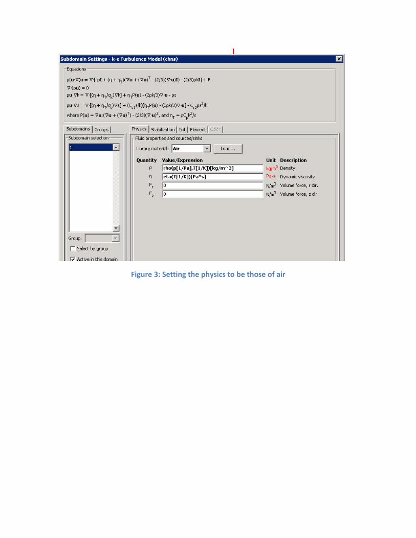
Figure 3: Setting the physics to be those of air

Figure 4: Setting the initial conditions to the system
The pressure was input as a boundary condition at the outlet, while the inlet condition was the
velocity of the fluid flowing through the pipe. The central wall was set to be axially symmetric
so as to provide a 3-D simulation of the pipe while showing a 2-D rectangle.

Figure 5: Setting the inlet boundary condition to velocity

Figure 6: Setting the outlet boundary setting to be pressure
Once all the inputs were made correctly, the mesh of the object was defined and then refined
in order to more accurately predict how the fluid would act in the pipe. The mesh was refined
most specifically at the wall since the closer you get to the wall the more unpredictable the
fluid becomes. The inlet mesh was also refined greatly in order to more accurately predict the
way the pipe would act in real life.

Figure 7: Refining the mesh at the wall
With the different values put into the system, the model can be run for different experiments.
The results were examined using the post-processing techniques included with the program,
specifically a boundary integration of pressure across several of the boundaries as well as a
velocity profile. These are shown below.

Figure 8: Color variance shown in the model’s display of pressure drop across the model
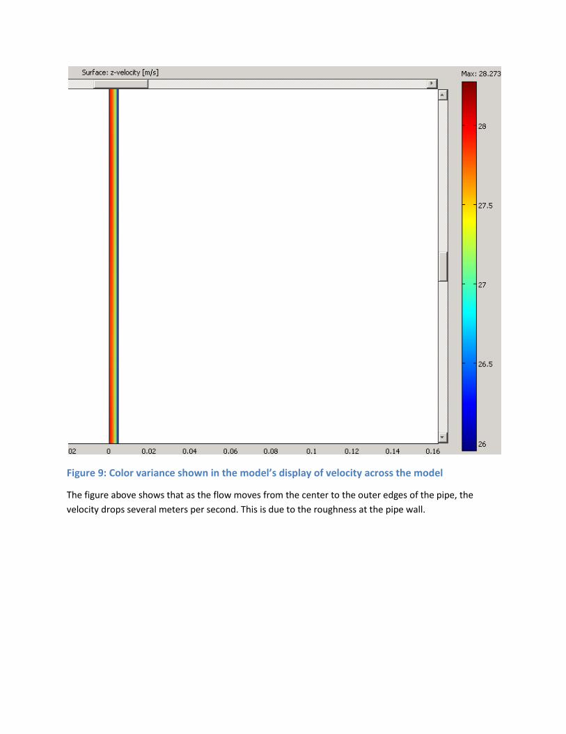
Figure 9: Color variance shown in the model’s display of velocity across the model
The figure above shows that as the flow moves from the center to the outer edges of the pipe, the
velocity drops several meters per second. This is due to the roughness at the pipe wall.

Figure 10: Boundary Integration feature of the Post-Processing function

Figure 11: Layout of Experimental Loop
24
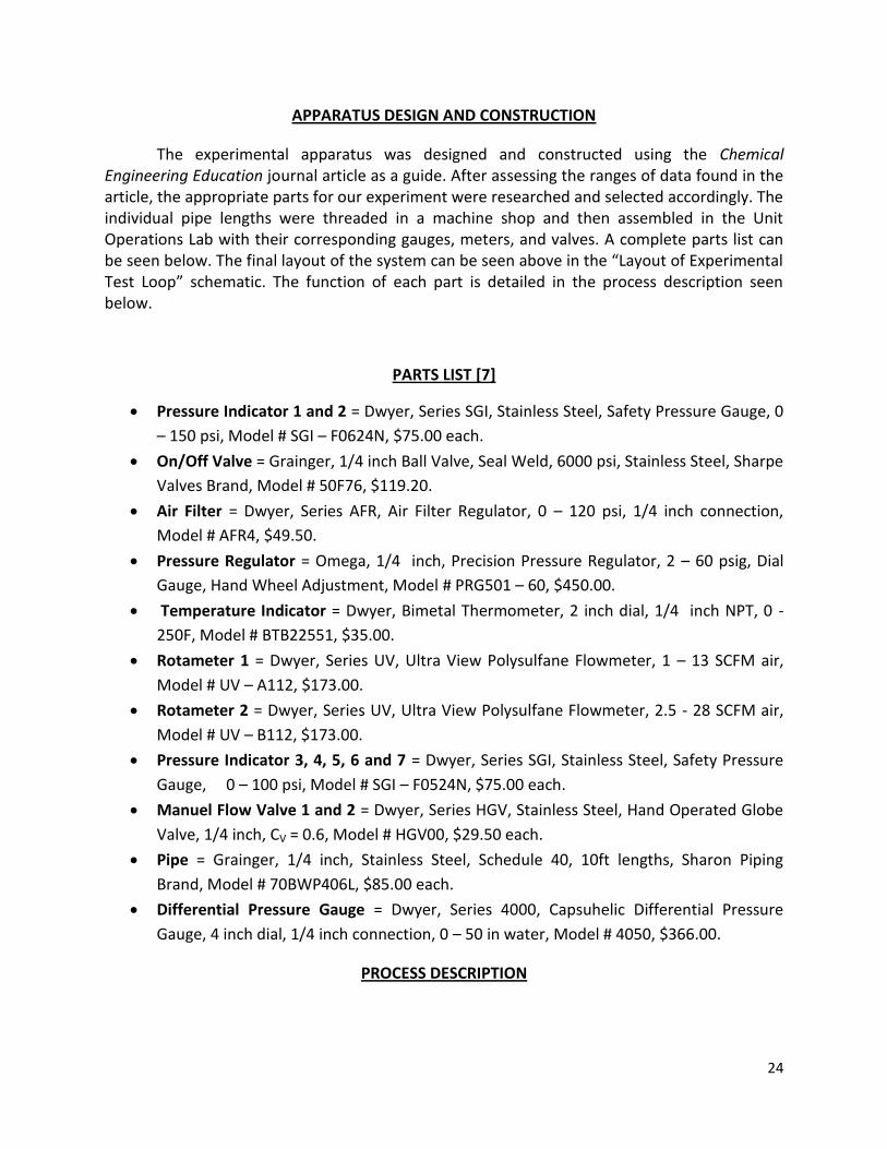
APPARATUS DESIGN AND CONSTRUCTION
The experimental apparatus was designed and constructed using the Chemical Engineering Education journal article as a guide. After assessing the ranges of data found in the article, the appropriate parts for our experiment were researched and selected accordingly. The individual pipe lengths were threaded in a machine shop and then assembled in the Unit Operations Lab with their corresponding gauges, meters, and valves. A complete parts list can be seen below. The final layout of the system can be seen above in the “Layout of Experimental Test Loop” schematic. The function of each part is detailed in the process description seen below.
PARTS LIST [7]
Pressure Indicator 1 and 2 = Dwyer, Series SGI, Stainless Steel, Safety Pressure Gauge, 0
– 150 psi, Model # SGI – F0624N, $75.00 each.
On/Off Valve = Grainger, 1/4 inch Ball Valve, Seal Weld, 6000 psi, Stainless Steel, Sharpe
Valves Brand, Model # 50F76, $119.20.
Air Filter = Dwyer, Series AFR, Air Filter Regulator, 0 – 120 psi, 1/4 inch connection,
Model # AFR4, $49.50.
Pressure Regulator = Omega, 1/4 inch, Precision Pressure Regulator, 2 – 60 psig, Dial
Gauge, Hand Wheel Adjustment, Model # PRG501 – 60, $450.00.
Temperature Indicator = Dwyer, Bimetal Thermometer, 2 inch dial, 1/4 inch NPT, 0 -
250F, Model # BTB22551, $35.00.
Rotameter 1 = Dwyer, Series UV, Ultra View Polysulfane Flowmeter, 1 – 13 SCFM air,
Model # UV – A112, $173.00.
Rotameter 2 = Dwyer, Series UV, Ultra View Polysulfane Flowmeter, 2.5 - 28 SCFM air,
Model # UV – B112, $173.00.
Pressure Indicator 3, 4, 5, 6 and 7 = Dwyer, Series SGI, Stainless Steel, Safety Pressure
Gauge, 0 – 100 psi, Model # SGI – F0524N, $75.00 each.
Manuel Flow Valve 1 and 2 = Dwyer, Series HGV, Stainless Steel, Hand Operated Globe
Valve, 1/4 inch, CV = 0.6, Model # HGV00, $29.50 each.
Pipe = Grainger, 1/4 inch, Stainless Steel, Schedule 40, 10ft lengths, Sharon Piping
Brand, Model # 70BWP406L, $85.00 each.
Differential Pressure Gauge = Dwyer, Series 4000, Capsuhelic Differential Pressure
Gauge, 4 inch dial, 1/4 inch connection, 0 – 50 in water, Model # 4050, $366.00.
PROCESS DESCRIPTION
25
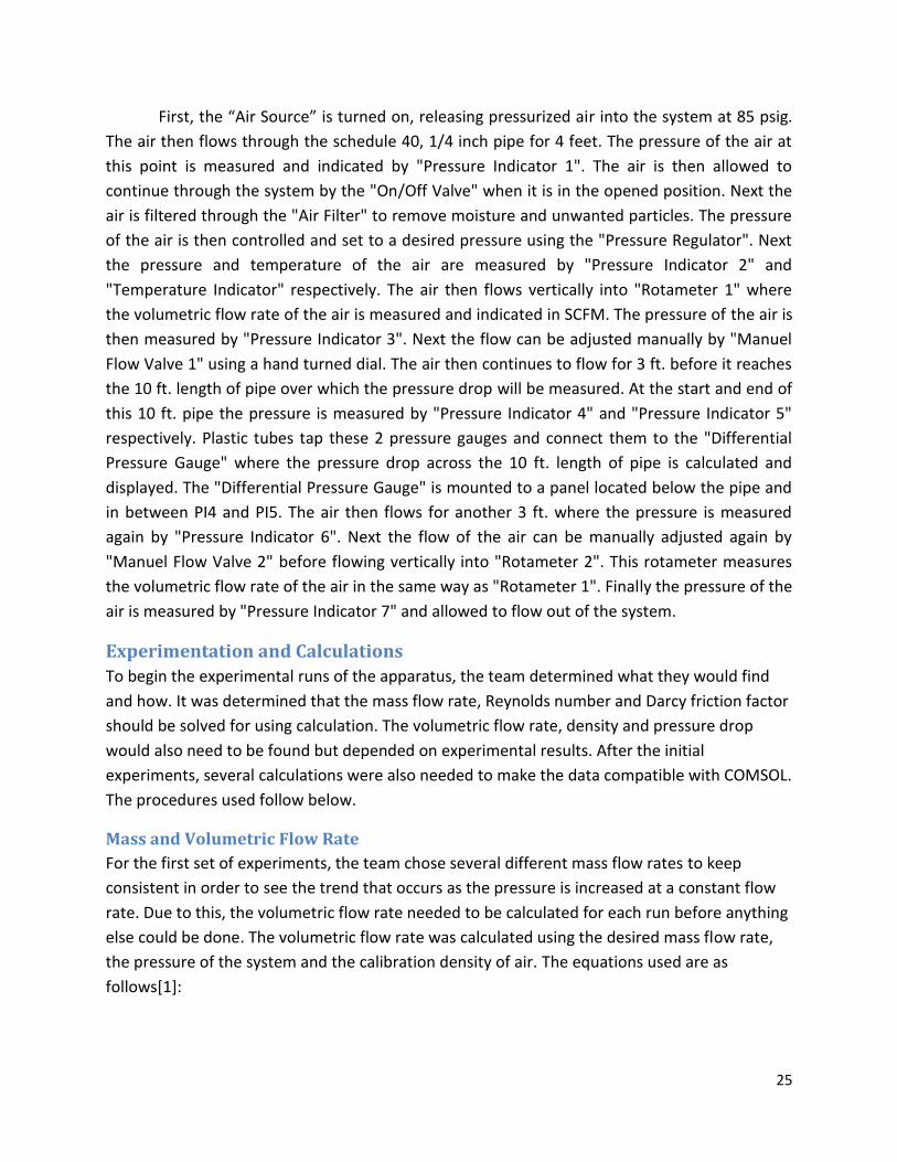
First, the “Air Source” is turned on, releasing pressurized air into the system at 85 psig.
The air then flows through the schedule 40, 1/4 inch pipe for 4 feet. The pressure of the air at
this point is measured and indicated by "Pressure Indicator 1". The air is then allowed to
continue through the system by the "On/Off Valve" when it is in the opened position. Next the
air is filtered through the "Air Filter" to remove moisture and unwanted particles. The pressure
of the air is then controlled and set to a desired pressure using the "Pressure Regulator". Next
the pressure and temperature of the air are measured by "Pressure Indicator 2" and
"Temperature Indicator" respectively. The air then flows vertically into "Rotameter 1" where
the volumetric flow rate of the air is measured and indicated in SCFM. The pressure of the air is
then measured by "Pressure Indicator 3". Next the flow can be adjusted manually by "Manuel
Flow Valve 1" using a hand turned dial. The air then continues to flow for 3 ft. before it reaches
the 10 ft. length of pipe over which the pressure drop will be measured. At the start and end of
this 10 ft. pipe the pressure is measured by "Pressure Indicator 4" and "Pressure Indicator 5"
respectively. Plastic tubes tap these 2 pressure gauges and connect them to the "Differential
Pressure Gauge" where the pressure drop across the 10 ft. length of pipe is calculated and
displayed. The "Differential Pressure Gauge" is mounted to a panel located below the pipe and
in between PI4 and PI5. The air then flows for another 3 ft. where the pressure is measured
again by "Pressure Indicator 6". Next the flow of the air can be manually adjusted again by
"Manuel Flow Valve 2" before flowing vertically into "Rotameter 2". This rotameter measures
the volumetric flow rate of the air in the same way as "Rotameter 1". Finally the pressure of the
air is measured by "Pressure Indicator 7" and allowed to flow out of the system.
Experimentation and Calculations
To begin the experimental runs of the apparatus, the team determined what they would find
and how. It was determined that the mass flow rate, Reynolds number and Darcy friction factor
should be solved for using calculation. The volumetric flow rate, density and pressure drop
would also need to be found but depended on experimental results. After the initial
experiments, several calculations were also needed to make the data compatible with COMSOL.
The procedures used follow below.
Mass and Volumetric Flow Rate
For the first set of experiments, the team chose several different mass flow rates to keep
consistent in order to see the trend that occurs as the pressure is increased at a constant flow
rate. Due to this, the volumetric flow rate needed to be calculated for each run before anything
else could be done. The volumetric flow rate was calculated using the desired mass flow rate,
the pressure of the system and the calibration density of air. The equations used are as
follows[1]:

26
(6)
(7)
Where F is the flow rate and the super scripts mass and vol stand for either mass flow rate or
volumetric flow rate. The volumetric flow rate term is calculated, not calibration. The ρcal term
is the density of air used to calibrate the rotameters. This term is calculated using standard
temperature and pressure and remains constant throughout the experiments.
For this experiment’s purposes, the actual mass flow rate was set prior. This value was used
with the difference in pressures to find the calibration mass flow rate. The calibration mass flow
rate was then used along with the calibration density of air to calculate the volumetric flow
rate.
The volumetric flow rate calculated was then used as a starting point for each experiment. The
rotameter was set to these values and the pressure drop between the rotameter and the ten
foot length of pipe was recorded. This provided approximately the actual pressure that the
system would be operating at. Using the difference in pressures then, the volumetric flow rate
for the rotameter was set so that the corrected volumetric flow rate would be the one specified
earlier to have a certain mass flow rate. The equation used is shown below[1]:
(8)
Where Q2 is the volumetric flow rate at the ten foot pipe, Q1 is the volumetric flow rate at the
rotameter, and each P is the corresponding pressure to those locations. This equation differs
from equation six in that it is volumetric flow rate and it also solves the equation between two
experimental pressures while equation six finds a pressure based on the values used to
calibrate the rotameter.
Pressure Drop
The pressure drop across the ten foot length of pipe in the experiment was determined using
the differential pressure gauge installed on the system. This value was then multiplied by 27.7
in order to get the pressure drop in pounds per square inch. This was necessary to compare this
experiment’s results with those in the chemical engineering journal. These values were also
used in creating a graphical representation of the data.

27
Density
The density of air in each individual experiment was calculated using a variation of the ideal gas
law that includes density. For this calculation, the pressure directly after the rotameter was
taken to ensure the density was calculated using the pressure closest to the ten foot length of
pipe [1].
(9)
Entry Length
The entry length for the pipe needed to be calculated for each experiment to determine what
length of pipe would lead up to the ten foot length. This entry length would provide that the
flow of air in the pipe would be fully developed flow and therefore turbulent. Having fully
developed flow was a necessity to be sure the experimental results would be consistent from
run to run. The equation used is shown below [2].
(10)
Where L is the entry length, Re is the Reynolds number and D is the diameter of the pipe.
Calculating values for COMSOL from Experimental Results
In order to make comparisons between COMSOL and the experiments performed in lab, the
correct values for pressure and velocity needed to be calculated prior to entering them into
COMSOL.
Velocity
COMSOL has a default to require a velocity in meters per second. In order to solve for this a
calculation was done involving several conversion factors, the cross-sectional area of the pipe
and the corrected volumetric flow rate. The equation used is shown below [2]:
(11)
Where V is velocity, A is cross sectional area, F is the corrected volumetric flow rate ft^3/min,
1/60 is a conversion from minutes to seconds and 1/3.048 is a conversion from feet to meters.
Pressure
The default units for pressure in COMSOL are pascals, and the pressure is an absolute pressure.
As such the pressure given by the apparatus must be converted to be the same. The equation
used is shown below [4]:
(12)

28
Where Ppa is the absolute pressure in pascals, Ppsi is the gauge pressure in psi, 6894 is the
number of pascals in a psi and 101325 is the number of pascals at atmospheric pressure.

29
Results and Discussion
Experimental Results
Once completing the experiment, the group plotted the pressure of the flow versus the
pressure drop at different flow rates. Because the goal of the experiment was to match up
these new results with the published document, the data from the other document is also
plotted in the figure below.
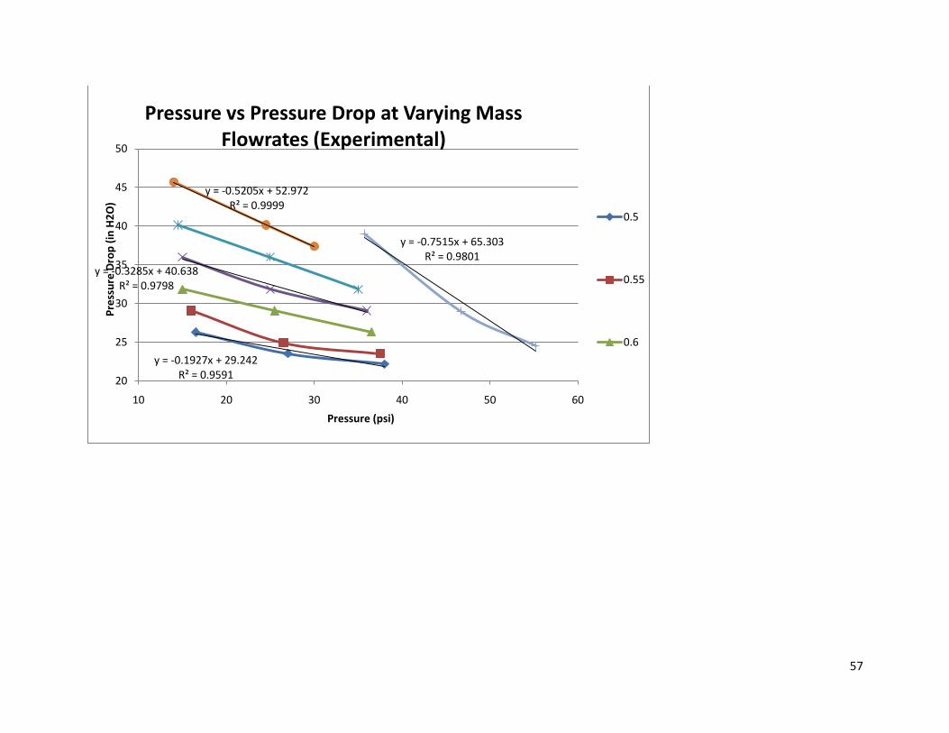
Figure 12: Pressure vs. Pressure Drop at Varying Mass Flowrates (Experimental)
As can be seen in the plot above, there is an obvious trend where the pressure drop decreases
with increasing pressure. As the mass flow rate rises, the amount of pressure drop in the flow
decreases at an increasing rate as the pressure increases. This is because with an increasing
mass flow rate, the velocity increases. With a higher pressure, the density increases and the
velocity decreases. Because velocity has more of an effect on the pressure drop than the
density, the pressure drop at higher mass flow rates declines at a noticeably higher rate.
Due to limitations with the apparatus that was constructed, it was not possible to attain data at
the mass flow rate used in the document that was being emulated. Mass flow rates at the same
pressures were also very difficult to obtain due to limitations. In trying to attain a mass flow
rate at a very high pressure, the volumetric flow rate would rise to the point that there was no
y = -0.1927x + 29.242R² = 0.9591
y = -0.5205x + 52.972R² = 0.9999
y = -0.7515x + 65.303R² = 0.9801
20
25
30
35
40
45
50
10 20 30 40 50 60
Pre
ssu
re D
rop
(in
H2
O)
Pressure (psi)
0.5
0.55
0.6
0.65
0.7
0.75
0.83

30
back pressure and the pressure within the system would drop. In trying to get a mass flow rate
high enough to compare to the paper, the team decided to use three pressures that would be
applicable at many different mass flow rates and try to get as close to the paper’s data as
possible. Thus the higher pressures that the paper used were not applicable to this apparatus.
At the pressures in the paper, the low mass flow rates would show essentially the same
pressure drops to other mass flow rates given the same trends.
In the graph above, the data for 0.83 lbm/min is at pressures of roughly one atmosphere, or
14.7 pounds per square inch, higher than the team’s data. However, one can see that if the
data was recorded at the pressures the team used and still followed the same trend line, it
would fit well with the data attained by the team. The flow rate is slightly higher than the
highest flow rate that the team used, and the rate at which the pressure drop decreases is also
slightly higher than that of 0.75 lbm/min. If a new pressure regulator could be purchased, then it
is very possible that the experiment could be repeated and fit the trend well.
COMSOL Results
Once the COMSOL model was fully set up, it was run several times for each experimental run in
the lab. The velocity and the pressure that were calculated from experimental data for use
within the model were input for each situation and the results produced several trends.
Figure 13: Pressure vs. Pressure Drop at Varying Mass Flowrates (COMSOL)
25
30
35
40
45
50
55
0 10 20 30 40
Pre
ssu
re D
rop
(in
H2
O)
Pressure (psi)
0.5
0.6
0.65
0.7

31
As can be seen in the above graph, the COMSOL data shows the same general trend as the
experimental data when it comes to pressure vs. pressure drop. As the pressure of the system
increases, the pressure drop across the pipe decreases. This is exhibited more closely in the
graph below which shows only the runs at 0.65 and 0.7 lb/min.
Figure 14: Pressure vs. Pressure Drop at 0.65 and 0.7 lb/min (COMSOL)
A second trend that should be noted is that as the velocity increased within a constant mass
flow rate, the pressure drop also increased. An increase in velocity in the system coincides with
a decrease in pressure, so this makes sense on both accounts.
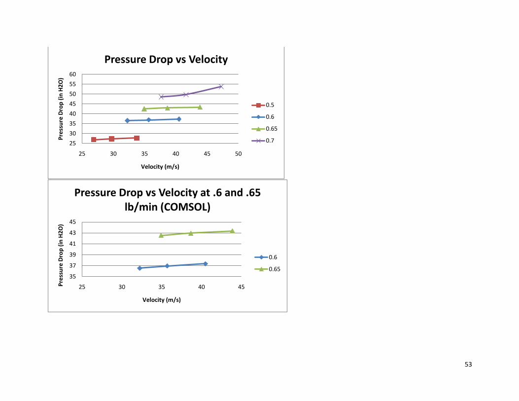
Figure 15: Pressure Drop vs. Velocity at Varying Flow Rates
40
42
44
46
48
50
52
54
0 10 20 30 40
Pre
ssu
re D
rop
(in
H2
O)
Pressure (psi)
0.7
0.65
25
30
35
40
45
50
55
60
25 30 35 40 45 50
Pre
ssu
re D
rop
(in
H2
O)
Velocity (m/s)
0.5
0.6
0.65
0.7

32
As can be seen above and more closely below, there is a clear trend in the pressure drop
getting larger as the velocity in the system increases.
Figure 16: Pressure Drop vs. Velocity at 0.6 and 0.65 lb/min (COMSOL)
Differences between Mass Flow Rates
When looking at the data acquired from running the experiment, the group found that while
keeping a constant mass flow rate and setting the pressure regulator to a certain pressure,
there would be a certain pressure drop across the pipe. If the pressure regulator was set to a
lower pressure while keeping the mass flow rate the same, the pressure drop would rise. If the
reverse was to be done, raising the pressure and keeping the mass flow rate the same, the
pressure drop would decrease from its previous value.
If the set pressure is lowered, then the compressible gas would have a higher velocity through
the pipe. The higher the velocity becomes, the more the pressure drop increases due to its part
in the pressure drop formula [2]:
(13)
As is shown above, the velocity is squared in the equation for pressure drop. This counteracts
the friction factor and density decreasing as the pressure drops, and causes the overall pressure
drop across the pipe to increase.
If the mass flow rate was increased while keeping the same pressure, the pressure drop would
increase as well. Following that trend, if the mass flow rate was decreased the pressure drop
would decrease as well. This is because as the mass flow rate is increased the velocity is also
35
36
37
38
39
40
41
42
43
44
25 30 35 40 45
Pre
ssu
re D
rop
(in
H2
O)
Velocity (m/s)
0.6
0.65

33
increased, and as the explanation above tells, the pressure drop will rise as the velocity
increases.
Rotameter Inaccuracy
When calculating the experimental results, the team came across a problem. The two
rotameters were reading different volumetric flow rates. After use of the below equation, it
became clear that the two rotameters disagreed greatly on what the flow rate was. The team
based all its calculations on the reading of the first rotameter to avoid any undue differences in
the numbers [1].
(14)
The inaccuracy of the second rotameter is shown on the graph below. The rotameter
consistently read higher than what it should have to represent what the flow rate was through
the pipe.
Figure 17: 2nd Rotameter Inaccuracy at 0.5 lb/min
COMSOL Results vs. Experimental Results
The COMSOL and experimental results showed many of the same trends. The main difference is
that the experimental results show a much more dramatic change in pressure drop when the
pressure is changed. This is shown in the following graphs.
5
5.5
6
6.5
7
7.5
1.2 1.4 1.6 1.8
Vo
lum
etr
ic F
low
Rat
e (
SCFM
)
Pressure (psig)
What we should see
What is shown

34
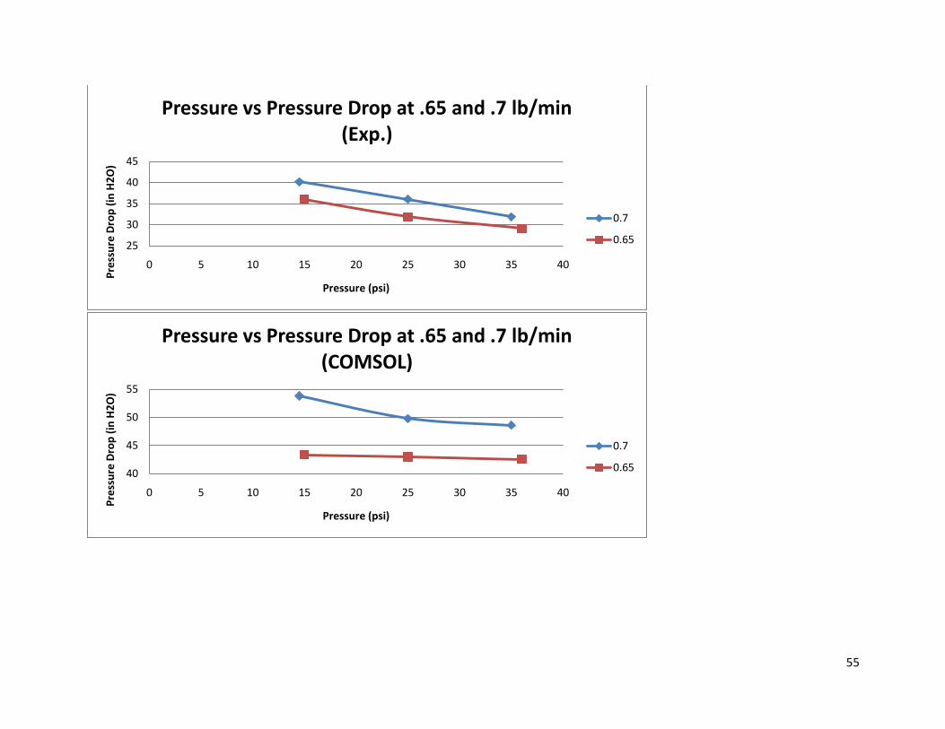
Figure 18: Pressure vs. Pressure Drop at 0.65 and 0.7 lb/min (COMSOL)
Figure 19: Pressure vs. Pressure Drop at 0.65 and 0.7 lb/min (Experimental)
As the above graphs show, the pressure drop is higher in the COMSOL model. The data also
shows that as the pressure is increased, the pressure drop across the pipe rises. While this
trend is shown by both sets of data, the COMSOL data at a mass flow of 0.65 lb/min drops 1
inch of water and the experimental data show a drop of 8 inches of water for the same
pressures and flow rate. These two sets of data are shown below in the same graph for
comparison.
40
42
44
46
48
50
52
54
0 10 20 30 40
Pre
ssu
re D
rop
(in
H2
O)
Pressure (psi)
0.7
0.65
25
27
29
31
33
35
37
39
41
43
45
0 10 20 30 40
Pre
ssu
re D
rop
(in
H2
O)
Pressure (psi)
0.7
0.65

35
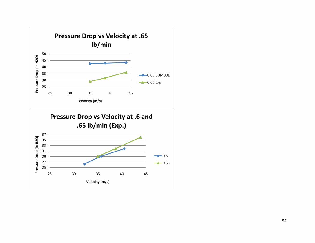
Figure 20: Pressure vs. Pressure Drop at 0.65 lb/min COMSOL vs. Experimental The same comparison can be made using pressure drop versus velocity in the COMSOL and
experimental data. As the velocity increases, so too does the pressure drop. While both sets of
data show this trend, the experimental data once again has a greater difference between each
datum. These data are shown below. The third graph shows a comparison between the
experimental and COMSOL data at the same mass flow rate.
Figure 21: Pressure Drop vs. Velocity at .6 and .65 lb/min (COMSOL)
25
27
29
31
33
35
37
39
41
43
45
0 10 20 30 40
Pre
ssu
re D
rop
(in
H2
O)
Pressure (psi)
0.65 COMSOL
0.65 Exp
35
36
37
38
39
40
41
42
43
44
25 30 35 40 45
Pre
ssu
re D
rop
(in
H2
O)
Velocity (m/s)
0.6
0.65

36
Figure 22: Pressure Drop vs. Velocity at 0.6 and 0.65 lb/min (Experimental)
Figure 23: Pressure Drop vs. Velocity at 0.65 lb/min COMSOL vs. Experimental
Reynolds Number
In order to calculate the Darcy friction factor and pressure drop of the flow, the Reynolds
number must first be determined. Using the equation for finding the Reynolds number found in
the background of this document, the results for each flow can be seen in the table below.
25
27
29
31
33
35
37
25 30 35 40 45
Pre
ssu
re D
rop
(in
H2
O)
Velocity (m/s)
0.6
0.65
25
30
35
40
45
50
25 30 35 40 45
Pre
ssu
re D
rop
(in
H2
O)
Velocity (m/s)
0.65 COMSOL
0.65 Exp

37
Table 1: Reynolds Numbers at varying Densities and Velocities
Flow Rate (lbm/min)
Pressure (psi)
Density (lbm/ft^3)
Velocity (ft/sec)
Diameter (ft)
Dynamic Viscosity
(lbf*s/ft^2)
Reynolds Number
0.5 38 1.936E-01 59.6 3.03E-02 3.82E-07 28464
0.5 27 1.376E-01 83.8 3.03E-02 3.82E-07 28464
0.5 16.5 8.408E-02 137.2 3.03E-02 3.82E-07 28464
0.55 37.5 1.911E-01 66.4 3.03E-02 3.82E-07 31310
0.55 26.5 1.350E-01 93.9 3.03E-02 3.82E-07 31310
0.55 16 8.153E-02 155.6 3.03E-02 3.82E-07 31310
0.6 36.5 1.860E-01 74.4 3.03E-02 3.82E-07 34157
0.6 25.5 1.299E-01 106.5 3.03E-02 3.82E-07 34157
0.6 15 7.643E-02 181.0 3.03E-02 3.82E-07 34157
0.65 36 1.834E-01 81.7 3.03E-02 3.82E-07 37003
0.65 25 1.274E-01 117.7 3.03E-02 3.82E-07 37003
0.65 15 7.643E-02 196.1 3.03E-02 3.82E-07 37003
0.7 35 1.783E-01 90.5 3.03E-02 3.82E-07 39849
0.7 25 1.274E-01 126.7 3.03E-02 3.82E-07 39849
0.7 14.5 7.389E-02 218.5 3.03E-02 3.82E-07 39849
At each flow rate in the range of 0.5 lbm/min to 0.7 lbm/min, it is evident that the flow is
turbulent. As the flow rate increases, the Reynolds number also increases. Using these Reynolds
numbers, the Darcy friction factor can now be found.
Darcy Friction Factor
The Darcy friction factor is an important quantity used in the calculation for pressure drop. It
can be calculated using several methods:
1. Using a Moody diagram
2. The Colebrook Equation
3. The Haaland Equation
4. The Swamee-Jain Equation
Depending on the importance of time and accuracy, the desire to use each method could
change.
1. Moody diagram
Using a Moody diagram factor is by far the quickest and easiest method in determining
the Darcy friction factor, though it is the least accurate. Using the Reynolds number as
well as the relative roughness of the pipe, the friction factor can be found by following
38
the curves on the chart. Because the pipe is made of stainless steel, the roughness was
determined to be 4.92E-5 feet, giving a relative roughness of 0.0015. Using this method,
the friction factors all vary from around 0.026 to 0.027, but since the points are so close
together it is impossible to have more accurate results from just looking at the chart.
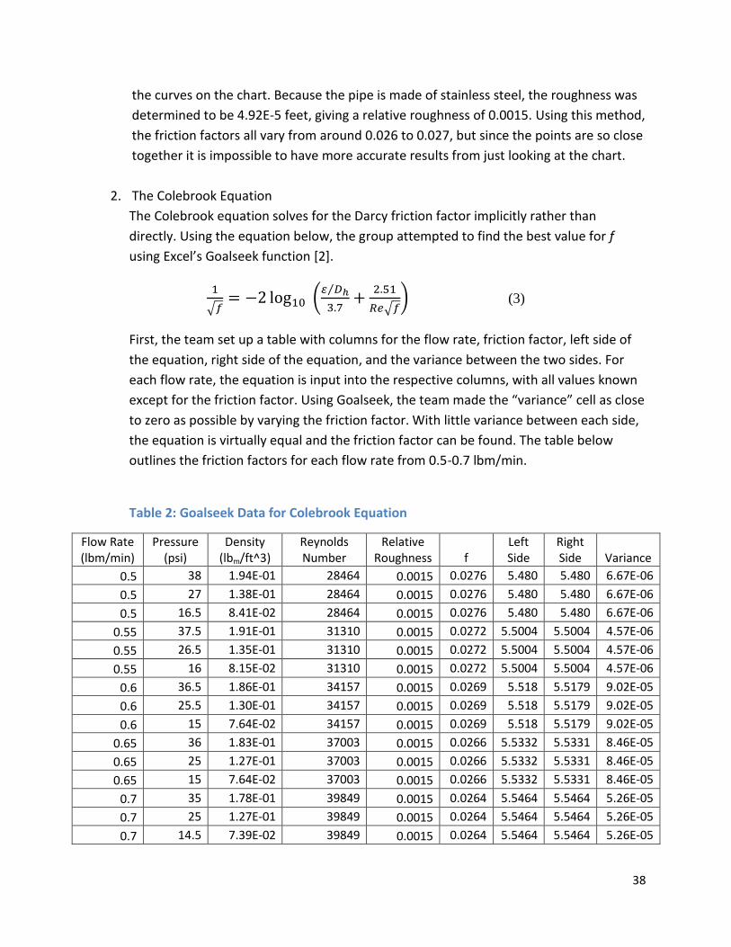
2. The Colebrook Equation
The Colebrook equation solves for the Darcy friction factor implicitly rather than
directly. Using the equation below, the group attempted to find the best value for f
using Excel’s Goalseek function [2].
(3)
First, the team set up a table with columns for the flow rate, friction factor, left side of
the equation, right side of the equation, and the variance between the two sides. For
each flow rate, the equation is input into the respective columns, with all values known
except for the friction factor. Using Goalseek, the team made the “variance” cell as close
to zero as possible by varying the friction factor. With little variance between each side,
the equation is virtually equal and the friction factor can be found. The table below
outlines the friction factors for each flow rate from 0.5-0.7 lbm/min.
Table 2: Goalseek Data for Colebrook Equation
Flow Rate (lbm/min)
Pressure (psi)
Density (lbm/ft^3)
Reynolds Number
Relative Roughness f
Left Side
Right Side Variance
0.5 38 1.94E-01 28464 0.0015 0.0276 5.480 5.480 6.67E-06
0.5 27 1.38E-01 28464 0.0015 0.0276 5.480 5.480 6.67E-06
0.5 16.5 8.41E-02 28464 0.0015 0.0276 5.480 5.480 6.67E-06
0.55 37.5 1.91E-01 31310 0.0015 0.0272 5.5004 5.5004 4.57E-06
0.55 26.5 1.35E-01 31310 0.0015 0.0272 5.5004 5.5004 4.57E-06
0.55 16 8.15E-02 31310 0.0015 0.0272 5.5004 5.5004 4.57E-06
0.6 36.5 1.86E-01 34157 0.0015 0.0269 5.518 5.5179 9.02E-05
0.6 25.5 1.30E-01 34157 0.0015 0.0269 5.518 5.5179 9.02E-05
0.6 15 7.64E-02 34157 0.0015 0.0269 5.518 5.5179 9.02E-05
0.65 36 1.83E-01 37003 0.0015 0.0266 5.5332 5.5331 8.46E-05
0.65 25 1.27E-01 37003 0.0015 0.0266 5.5332 5.5331 8.46E-05
0.65 15 7.64E-02 37003 0.0015 0.0266 5.5332 5.5331 8.46E-05
0.7 35 1.78E-01 39849 0.0015 0.0264 5.5464 5.5464 5.26E-05
0.7 25 1.27E-01 39849 0.0015 0.0264 5.5464 5.5464 5.26E-05
0.7 14.5 7.39E-02 39849 0.0015 0.0264 5.5464 5.5464 5.26E-05

39
As can be seen in the table above, as the flow rate increases the friction factor
decreases. This is because with more flow and a higher Reynolds number, the force of
friction on the flow by the walls of the pipe will have less of an effect on the flow, and
will be less of an influence on the pressure drop.
3. The Haaland Equation
Unlike the Colebrook equation, the Haaland equation can be solved directly and does
not require Goalseek to find the friction factor. In this way it is much quicker to use
than the Colebrook method [17].
(4)
The table below outlines the results of using the Haaland equation to find the friction
factor.
Table 3: Friction Factor Data for Haaland Equation
Flow Rate (lbm/min)
Pressure (psi) Density
Reynolds Number
Relative Roughness
f (Haaland)
0.5 38 1.94E-01 28464 0.0015 0.0272
0.5 27 1.38E-01 28464 0.0015 0.0272
0.5 16.5 8.41E-02 28464 0.0015 0.0272
0.55 37.5 1.91E-01 31310 0.0015 0.0269
0.55 26.5 1.35E-01 31310 0.0015 0.0269
0.55 16 8.15E-02 31310 0.0015 0.0269
0.6 36.5 1.86E-01 34157 0.0015 0.0265
0.6 25.5 1.30E-01 34157 0.0015 0.0265
0.6 15 7.64E-02 34157 0.0015 0.0265
0.65 36 1.83E-01 37003 0.0015 0.0263
0.65 25 1.27E-01 37003 0.0015 0.0263
0.65 15 7.64E-02 37003 0.0015 0.0263
0.7 35 1.78E-01 39849 0.0015 0.0260
0.7 25 1.27E-01 39849 0.0015 0.0260
0.7 14.5 7.39E-02 39849 0.0015 0.0260
4. The Swamee-Jain Equation
Like the Haaland method above, the Swamee-Jain method solves directly for the
friction factor. It is also very quick and easy to use [18].
(5)

40
The following table outlines the team’s results for the Swamee-Jain equation.
Table 4: Friction Factor Data for Swamee-Jain Equation
Flow Rate (lbm/min)
Pressure (psi) Density
Reynolds Number
Relative Roughness f (Swamee-Jain)
0.5 38 1.94E-01 28464 0.0015 0.0278
0.5 27 1.38E-01 28464 0.0015 0.0278
0.5 16.5 8.41E-02 28464 0.0015 0.0278
0.55 37.5 1.91E-01 31310 0.0015 0.0274
0.55 26.5 1.35E-01 31310 0.0015 0.0274
0.55 16 8.15E-02 31310 0.0015 0.0274
0.6 36.5 1.86E-01 34157 0.0015 0.0271
0.6 25.5 1.30E-01 34157 0.0015 0.0271
0.6 15 7.64E-02 34157 0.0015 0.0271
0.65 36 1.83E-01 37003 0.0015 0.0268
0.65 25 1.27E-01 37003 0.0015 0.0268
0.65 15 7.64E-02 37003 0.0015 0.0268
0.7 35 1.78E-01 39849 0.0015 0.0266
0.7 25 1.27E-01 39849 0.0015 0.0266
0.7 14.5 7.39E-02 39849 0.0015 0.0266
5. Comparison between all methods
Looking at the results from all of the methods, it is clear that some methods are better for
different situations. The figure below is a plot of the friction factor versus the log of the
Reynolds number for all of the methods.

41
Figure 24: Reynolds Number vs. Friction Factor for Various Calculation Methods
The Moody diagram, the first method used, gave results that were all between 0.026 and
0.027. Since all of the data from the three equations fell in that range, then it is evident
that the Moody diagram is a reliable source for finding the friction factor as long as the
result does not need to be more accurate. The Moody diagram is by far the quickest
method. The Colebrook equation, on the other side of the spectrum, is the longest and
most difficult to use. However, it is also the most accurate in finding the friction factor. The
Haaland equation gave results that were slightly lower than that of the Colebrook equation,
but was still accurate even though it solved directly for the friction factor. The Swamee-Jain
method gave results that were roughly 0.005 higher on all points than the Colebrook
method. It also solved directly for the friction factor, but is not as accurate as the Haaland
equation.
Entry Length
The entry length of the pipe for this system was calculated to be between .22 and .24
meters for the range of this experiment. That is equal to about a foot of pipe. The
experiment was built with close to three feet entrance length to be sure the flow would be
fully developed before it reached the ten foot length of pipe.
0.0255
0.026
0.0265
0.027
0.0275
0.028
4.4 4.45 4.5 4.55 4.6 4.65
Fric
tio
n F
acto
r
log10(Re)
Colebrook
Swamee-Jain
Haaland
42
Conclusions While the mass flow rate was kept constant during the first set of experiments, the volumetric
flow rate varied with the pressure due to the changes in gas density. As the gas density
decreased, the gas velocity increased through the rotameter which caused the volumetric flow
rate to rise. This will be a good phenomenon for students to explain and understand in the unit
operations laboratory.
The comparison between the experimental data and the chemical engineering journal article
showed that the apparatus constructed by the team accurately attained similar results to the
experiment it was modeled off. While the exact data could not be achieved, this was due to the
systems inability to simulate such high mass flow rates as were used in the original experiment.
The trend shown by the data accurately predicts the same data should the higher mass flow
rate have been achieved.
The density is the main value changing in this system to affect the results. This is caused by a
change in pressure. A higher pressure makes the fluid denser and slows it down, while a lower
pressure makes the fluid less dense and speeds it up. The higher the velocity, the more
pressure drop will be present across the pipe. Therefore, as density increases, pressure drop
across the pipe decreases.
The COMSOL model showed the same trends as the experimental results. The model had much
higher pressure drops across the pipe, and much less difference between pressure jumps. This
seems to indicate that the model cannot accurately predict the activity within the pipe. The
model can still be used to demonstrate the concepts of pressure drop across a length of pipe.
To show a class the trends of pressure drop across a pipe, a professor can use the COMSOL
model and it would be easier than taking them to lab to demonstrate.

43
Recommendations
To further develop the educational purposes of the Unit Operations labs, suggestion are added
to improve the quality of the experiment and test other subject matter that are applicable to
the apparatus.
2nd pipe
The team would suggest incorporating a second pipe into the system. A different sized pipe
would be optimal. This would give the laboratory experiment more time in lab, as well as giving
students a comparison between two different sizes of pipe. With two different sized pipes, the
students would have a better understanding of how pipe sizing affects turbulence and pressure
drop. In addition the use of alternative material which could range from PVC to copper tubing
would illustrate the effect of the smoothness of the pipe to pressure drop. The smoother the
pipe, the lower of a pressure loss will occur.
Rotameters
As was concluded from the team’s calculations between the two rotameters, they are
inaccurate with regard to one another. There is no way to tell if one is more accurate than the
other since the experimental calculations depend on that information. The team would
recommend that two of the same rotameter be used. This would mean either buying another
of the first rotameter, or buying two entirely new rotameters. This will be necessary to show
students that the following equation is appropriate for calculating the flow rate of the system
[2].
Without two rotameters that show the same flowrate, it will not be clear whether or not the
square root is necessary in calculating the flow rate.
Anemometers
Anemometers can be found in many of the engineering industries for the measurement of
velocity for fluid flow. For the purposes of this project anemometers can be placed at the end
of the piping unit for this determination. Despite the use of rotameters in the experiment it
was determined a large source of error was present due to the two in use showing significant
differences in mass flow rate reading. Using additional equipment will further ensure accurate
readings and can be used to calibrate the rotameters. There are multiple types of

44
anemometers available to sale, but for the purposes of the experiment hot-wire and rotating
anemometers will be further discuss.
Heat-wire anemometers utilize a two to three small thin strips of metal, which are located at
the end of the device. Due to the small size of the device, it can measure small piping units and
other constricted areas. The metal is usually made of platinum, tungsten or an alloy of these
components, which is heated to a temperature far above the ambient temperature [12]. Upon
the introduction of the gas flowing past the heated metal, the cooling effect of convection is
measured. This can be done through measuring the resistance which is dependent upon
temperature. The instrument is programmed to determine the wires resistance to the fluid
velocity. It is important to note that a constant flow or temperature is necessary for accurate
reading in the heat-wire anemometer. These anemometers typically range from 300 to 700
dollars, but can be in excess of a thousand dollars for the higher end models [11]. Despite the
advantages to using heat-wire a few problems are also present in these devices. Due to the
small and expensive metal which all the measurements are conducted they are easy to break if
not handled carefully. Also the supply of gas needs to be free of particulates; otherwise they
will accumulate on the wires. While this is not reversible, the wire must be overheated to rid
them from the surface.
The alternative anemometer is a rotation based dependent upon the power pressurized gas to
move the rotating part, which is recorded to determine the fluid velocity. The two rotating
anemometers, windmill and cup abide by the same basic principles but differ in design. This
style of equipment was developed far earlier in 1672, with Robert Hooke believed to create the
first working model. Price usually ranges from 100 to 300 dollars, and are a much more durable
product [8].
Heater
An additional modification to the Pressure Drop Unit Operations experiment is the use of a
heater. This tests the student’s ability to evaluate the effect of heat to pressure drop in a
piping system due to the heats effect upon changes in velocity and air density. From the lab it
should be concluded that an increase in temperature of the system will decrease density
causing a higher gas velocity. This increased velocity will increase the pressure drop across the
ten foot pipe.
There are many different ways to introduce heat into the system; the most effective system
would be a T type air process heat. The High Pressure Air (AHP) unit available at omega.com is
more than adequate to heat the piping, reaching outlet temperatures of up to 540°C [6]. With
the attachment of thermocouples on both sides of the heater will show the temperature rise in
the piping. The voltage necessary for outlet air temperatures at to the desired degree can be
calculated from the equation below.

45
Where:
SCFM is standard cubic feet per minute
ØT is the temperature rise in Fahrenheit from the inlet stream
Based upon the piping equipment limits, flows must range between 2 and 20 CFM, which falls
within the specifications of the experiment. The pricing of the heater is relatively inexpensive
with prices at or below 100 dollars. In regards to safety the heater could be a potential hazard
in the experiment with its high temperature capability, thus placement of controlling features
should be considered in the design.
Unit Operations Lab The following is what the team has put together to give to students in the unit operations
laboratory to complete an experiment on the compressible fluid apparatus:
What you need to record in the lab:
the chosen pressure of the air flowing through the pipes (using the pressure regulator)
the flow rate through the rotameters (both before and after pressure drop)
note the temperature of the air above the rotameter for reference
record the pressure drop across the pipe using the differential pressure gauge
Using the information obtained above you can calculate/verify the following:
pressure drop across the pipe (in inches of H2O)
the mass flow rate calibration value,
the volumetric flow rate in the pipe in SCFM,
the entry length of the pipe, L
the Reynolds number, Re
the friction factor in the pipe (a few different ways), f
Before starting the lab, draw a schematic of the apparatus, becoming familiar with the
equipment and carefully labeling all valves and meters. List all safety equipment and gear
needed to perform the laboratory experiment with explanation. Make a proper procedure
detailing the steps needed to complete the experiment(s). Each group should take
approximately 5-10 min beforehand and discuss the differences between compressible and
incompressible flow. Each group should pick a pressure and pick a mass flow rate to try to
calculate what they should be getting for a pressure drop along the given 10 foot section of the
pipe. With a mass flow rate in mind, a calculation must be made to determine what volumetric
46
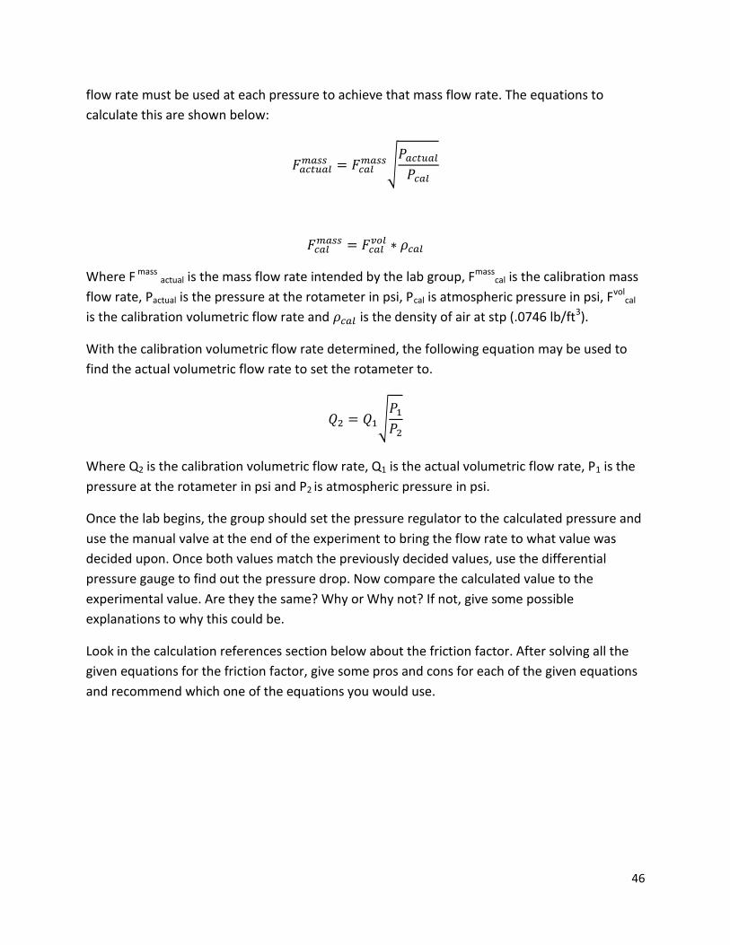
flow rate must be used at each pressure to achieve that mass flow rate. The equations to
calculate this are shown below:
Where F mass actual is the mass flow rate intended by the lab group, Fmasscal is the calibration mass
flow rate, Pactual is the pressure at the rotameter in psi, Pcal is atmospheric pressure in psi, Fvolcal
is the calibration volumetric flow rate and is the density of air at stp (.0746 lb/ft3).
With the calibration volumetric flow rate determined, the following equation may be used to
find the actual volumetric flow rate to set the rotameter to.
Where Q2 is the calibration volumetric flow rate, Q1 is the actual volumetric flow rate, P1 is the
pressure at the rotameter in psi and P2 is atmospheric pressure in psi.
Once the lab begins, the group should set the pressure regulator to the calculated pressure and
use the manual valve at the end of the experiment to bring the flow rate to what value was
decided upon. Once both values match the previously decided values, use the differential
pressure gauge to find out the pressure drop. Now compare the calculated value to the
experimental value. Are they the same? Why or Why not? If not, give some possible
explanations to why this could be.
Look in the calculation references section below about the friction factor. After solving all the
given equations for the friction factor, give some pros and cons for each of the given equations
and recommend which one of the equations you would use.
47
Calculation References: Students in the lab would also be given the following equations to use in their calculations in
the lab.
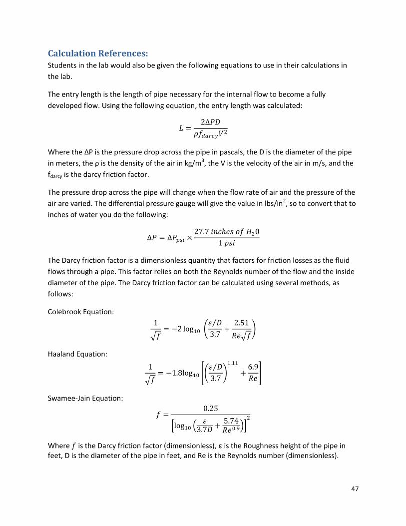
The entry length is the length of pipe necessary for the internal flow to become a fully
developed flow. Using the following equation, the entry length was calculated:
Where the ΔP is the pressure drop across the pipe in pascals, the D is the diameter of the pipe
in meters, the ρ is the density of the air in kg/m3, the V is the velocity of the air in m/s, and the
fdarcy is the darcy friction factor.
The pressure drop across the pipe will change when the flow rate of air and the pressure of the
air are varied. The differential pressure gauge will give the value in lbs/in2, so to convert that to
inches of water you do the following:
The Darcy friction factor is a dimensionless quantity that factors for friction losses as the fluid
flows through a pipe. This factor relies on both the Reynolds number of the flow and the inside
diameter of the pipe. The Darcy friction factor can be calculated using several methods, as
follows:
Colebrook Equation:
Haaland Equation:
Swamee-Jain Equation:
Where is the Darcy friction factor (dimensionless), ε is the Roughness height of the pipe in feet, D is the diameter of the pipe in feet, and Re is the Reynolds number (dimensionless).

48
The Reynolds number is the ratio of the inertial forces to the viscous forces and is used as a
measure to determine the type of flow inside the pipe. The equation used to calculate the
Reynolds number is:
Where the ρ is the density of the gas in lbm/ft3, the V is the velocity in ft/sec, the D is the
diameter in feet, the µ is the dynamic viscosity in lbf*s/ft2, and the gc is the gravity constant at
32.17 lbfft/lbmsec2.
The mass flow rate calibration value is used to find the calibration volumetric flow rate in the
pipe. The equation for the mass flow rate calibration value is:
Where the actual mass flow rate is the value assumed by the lab group, Pactual is the actual
pressure in psia, and the Pcal is the calibration pressure which is at ambient room pressure, or
14.7 psia.
The volumetric flow rate is calculated from the mass flow rate calibration value above over the
calibration density of the air, which in this case is 0.746.
49
References 1. Luyben, William L., and Kemal Tuzla. "Gas Pressure-Drop Experiment." Chemical Engineering
Education 44.3 (2010): 183-88. Print.
2. Fox, Robert W., Alan T. McDonald, and Philip J. Pritchard. Introduction to Fluid Mechanics. 7th
ed. Hoboken, NJ: Wiley, 2009. Print.
3. Moody diagram: http://people.msoe.edu/tritt/be382/MoodyChart.html
4. McCabe, Warren L., Julian C. Smith, and Peter Harriott. Unit Operations of Chemical Engineering.
7th ed. Boston: McGraw-Hill, 2005. Print.
5. www.COMSOL.com
6. Omega.com. Omega Engineering Inc. Web. 29 Mar. 2011.
7. "Dwyer Instruments Online Catalog." Dwyer Instruments Online. Web. 07 Nov. 2010.
<http://catalogs.dwyer-inst.com/WebProject.asp?CodeId=7.4.2.2>.
8. "Grainger Industrial Supply." Grainger Industrial Supply - MRO Supplies, MRO Equipment, Tools
& Solutions. Web. 10 Nov. 2010. <http://www.grainger.com/Grainger/wwg/viewCatalogPDF>.
9. Abel, Alan, Phil Lowe, Rachel Clair, and Daqian Wu. "Compressible Fluid Flow: Pressurizing and
Discharging of Tanks Under Adiabatic and Isothermal Conditions." Carnegie Mellon University,
22 May 2006. Web. 24 Mar. 2011.
<http://rothfus.cheme.cmu.edu/tlab/compflow/projects/t6s06/t6_s06_r3.pdf>.
10. Dutton, J. Craig, and Robert E. Coverdill. "Experiments to Study the Gaseous Discharge and
Filling of Vessels." International Journal of Engineering Education 13.2 (1997): 123-34. TEMPUS
Publications, 1997. Web. 23 Mar. 2011.
<http://www.akademik.unsri.ac.id/download/journal/files/ijee/ijee924.pdf>.
11. "Hot Wire Anemometers: Introduction." Efunda.com. 2011. Web. 18 Mar. 2011.
<http://www.efunda.com/designstandards/sensors/hot_wires/hot_wires_intro.cfm>.
12. "Hot Wire Anemometry." Annual Review of Fluid Mechanics 8 (1976): 209-
31.Annualreviews.org. Web of Science. Web. 25 Mar. 2011.
<http://www.annualreviews.org/doi/pdf/10.1146/annurev.fl.08.010176.001233>.
13. "Pipe Flow 3D - Pressure Drop Theory." Pipeflow.co.uk. Daxesoft Ltd. Web. 29 Mar. 2011.
<http://pipeflow.co.uk/public/control.php?_path=/417/503/510>.

50
14. Smith, J. M., H. C. Van Ness, and Michael M. Abbott. Introduction to Chemical Engineering
Thermodynamics. 7th ed. Boston: McGraw-Hill, 2005. Print.
15. "Fluid Pressure Drop Along Pipe Length of Uniform Diameter." Engineersedge.com. Engineers
Edge. Web. 1 Apr. 2011. <Engineersedge.com/fluid_flow/pressure_drop/pressure_drop.htm>.
16. Colebrook: Colebrook, C.F. (February 1939). "Turbulent flow in pipes, with particular reference
to the transition region between smooth and rough pipe laws". Journal of the Institution of Civil
Engineers (London).
17. Haaland: Haaland, S.E., 1983. Simple and explicit formulas for the friction factor in turbulent
pipe flow. J. Fluids Eng.
18. Swamee-Jain: Swamee, PK (1976). "Explicit equations for pipe-flow problems". Journal of the
Hydraulics Division (0044-796X), 102 (5), p. 657.

51
Appendix
ρcal 0.0746 Works for all experiments because it is the calibration value, not the calculated value
Area 0.000706858
Flow Rate (lb/min)Pressure (psi) F cal P2 Fvol reading P at vol 2 Fvol reading 2 Fvol Actual Delta P (psi) Delta P (in H2O)
0.5 40 0.2592 38 38 3.386553834 1.75 7 3.474530922 0.8 22.16
0.5 30 0.286731 27 27 3.646341476 1.5 6.7 3.843581397 0.85 23.545
0.5 20 0.325435 16.5 16.5 3.962343124 1.4 6.5 4.362396205 0.95 26.315
0.55 40 0.28512 37.5 37.5 3.700620109 2.1 7.5 3.821984014 0.85 23.545
0.55 30 0.315404 26.5 26.5 3.973663411 1.9 7.2 4.227939536 0.9 24.93
0.55 20 0.357978 16 16 4.292030362 1.6 6.8 4.798635825 1.05 29.085
0.6 40 0.31104 36.5 36.5 3.982849203 4.169437106 0.95 26.315
0.6 30 0.344077 25.5 25.5 4.252328347 2.25 7.8 4.612297676 1.05 29.085
0.6 20 0.390522 15 15 4.533535122 5.234875446 1.15 31.855
0.65 40 0.33696 36 36 4.284253774 4.516 1.05 29.085
0.65 30 0.372751 25 25 4.561616033 2.4 8 4.997 1.15 31.855
0.65 20 0.423065 15 15 4.911230065 5.671 1.3 36.01
0.7 40 0.36288 35 35 4.550176501 4.864343291 1.15 31.855
0.7 30 0.401424 25 25 4.912171209 5.381013955 1.3 36.01
0.7 20 0.455609 14.5 14.5 5.200225132 6.107354687 1.45 40.165
0.75 40 0.3888 30 30 4.513724405 5.212 1.35 37.395
0.75 30 0.430097 24.5 24.5 5.209808098 5.765 1.45 40.165
0.75 20 0.488152 14 14 5.475103214 6.544 1.65 45.705
0.85 40 0.44064 5.906702567 0
0.85 30 0.487443 6.534088374 2.05 56.785
0.85 20 0.553239 7.416073548 0
0.95 40 0.49248 6.601608752 0
0.95 30 0.544789 7.302804653 0
0.95 20 0.618326 8.288552789 0

52
Velocity (m/s) COMSOL P (Pa) COMSOL Delta P (Pa) Delta P exp (Pa) COMSOL Delta P (in H2O) sqrt of pressures
26.87265362 363272 6700 5520 26.89782 40 psi 1.929012
29.72695706 287438 6800 5865 27.29928 30 psi 1.743794
33.73956508 215051 6900 6555 27.70074 20 psi 1.536406
29.55991898 359825 8000 5865 32.1168
32.69965277 283991 8000 6210 32.1168
37.11352159 211604 8000 7245 32.1168
32.24718434 352931 9100 6555 36.53286
35.67234847 277097 9200 7245 36.93432
40.48747809 204710 9300 7935 37.33578
34.92756475 349484 10600 7245 42.55476
38.64770617 273650 10700 7935 42.95622
43.86054466 204710 10800 8970 43.35768
37.62171507 342590 12100 7935 48.57666
41.61773989 273650 12400 8970 49.78104
47.23539111 201263 13400 10005 53.79564
40.31055524 308120 12700 9315 50.98542
44.58755774 270203 14000 10005 56.2044
50.61248532 197816 14100 11385 56.60586
53
25
30
35
40
45
50
55
60
25 30 35 40 45 50
Pre
ssu
re D
rop
(in
H2
O)
Velocity (m/s)
Pressure Drop vs Velocity
0.5
0.6
0.65
0.7
35
37
39
41
43
45
25 30 35 40 45Pre
ssu
re D
rop
(in
H2
O)
Velocity (m/s)
Pressure Drop vs Velocity at .6 and .65 lb/min (COMSOL)
0.6
0.65
54
25
30
35
40
45
50
25 30 35 40 45Pre
ssu
re D
rop
(in
H2
O)
Velocity (m/s)
Pressure Drop vs Velocity at .65 lb/min
0.65 COMSOL
0.65 Exp
25
27
29
31
33
35
37
25 30 35 40 45Pre
ssu
re D
rop
(in
H2
O)
Velocity (m/s)
Pressure Drop vs Velocity at .6 and .65 lb/min (Exp.)
0.6
0.65
55
25
30
35
40
45
0 5 10 15 20 25 30 35 40
Pre
ssu
re D
rop
(in
H2
O)
Pressure (psi)
Pressure vs Pressure Drop at .65 and .7 lb/min (Exp.)
0.7
0.65
40
45
50
55
0 5 10 15 20 25 30 35 40
Pre
ssu
re D
rop
(in
H2
O)
Pressure (psi)
Pressure vs Pressure Drop at .65 and .7 lb/min (COMSOL)
0.7
0.65

56
25
30
35
40
45
50
55
0 10 20 30 40
Pre
ssu
re D
rop
(in
H2
O)
Pressure (psi)
Pressure vs Pressure Drop at Varying Mass Flowrates (COMSOL)
0.5
0.6
0.65
0.7
25
30
35
40
45
0 10 20 30 40
Pre
ssu
re D
rop
(in
H2
O)
Pressure (psi)
Pressure vs Pressure Drop at .65 COMSOL vs Exp.
0.65 COMSOL
0.65 Exp
57
y = -0.1927x + 29.242R² = 0.9591
y = -0.3285x + 40.638R² = 0.9798
y = -0.5205x + 52.972R² = 0.9999
y = -0.7515x + 65.303R² = 0.9801
20
25
30
35
40
45
50
10 20 30 40 50 60
Pre
ssu
re D
rop
(in
H2
O)
Pressure (psi)
Pressure vs Pressure Drop at Varying Mass Flowrates (Experimental)
0.5
0.55
0.6

58
Density
(lbm/ft^3
) Pressure
Flow
Rate
(lbm/min
)
Velocity
(ft/sec)
Diameter
(in)
Diameter
(ft)
Area
(in^2)
Area
(ft^2)
Dynamic
Viscosity
(lbf*s/ft^
2)
Kinemati
c
Viscosity
(ft^2/s)
Reynolds
number log10(Re)
roughnes
s e (ft)
0.193634 38 0.5 59.5535 0.364 0.030333 0.104062 0.000723 3.82E-07 6.35E-05 2.85E+04 4.454294 4.92E-05
0.137582 27 0.5 83.81604 0.364 0.030333 0.104062 0.000723 3.82E-07 8.93E-05 28463.89 4.454294 4.92E-05
0.084078 16.5 0.5 137.1535 0.364 0.030333 0.104062 0.000723 3.82E-07 1.46E-04 28463.89 4.454294 4.92E-05
0.191086 37.5 0.55 66.3823 0.364 0.030333 0.104062 0.000723 3.82E-07 6.43E-05 31310.28 4.495687 4.92E-05
0.135034 26.5 0.55 93.93722 0.364 0.030333 0.104062 0.000723 3.82E-07 9.10E-05 31310.28 4.495687 4.92E-05
0.08153 16 0.55 155.5835 0.364 0.030333 0.104062 0.000723 3.82E-07 1.51E-04 31310.28 4.495687 4.92E-05
0.18599 36.5 0.6 74.40109 0.364 0.030333 0.104062 0.000723 3.82E-07 6.61E-05 34156.67 4.533476 4.92E-05
0.129939 25.5 0.6 106.4957 0.364 0.030333 0.104062 0.000723 3.82E-07 9.46E-05 34156.67 4.533476 4.92E-05
0.076434 15 0.6 181.0426 0.364 0.030333 0.104062 0.000723 3.82E-07 1.61E-04 34156.67 4.533476 4.92E-05
0.183443 36 0.65 81.72064 0.364 0.030333 0.104062 0.000723 3.82E-07 6.70E-05 37003.06 4.568238 4.92E-05
0.127391 25 0.65 117.6777 0.364 0.030333 0.104062 0.000723 3.82E-07 9.65E-05 37003.06 4.568238 4.92E-05
0.076434 15 0.65 196.1295 0.364 0.030333 0.104062 0.000723 3.82E-07 1.61E-04 37003.06 4.568238 4.92E-05
0.178347 35 0.7 90.52132 0.364 0.030333 0.104062 0.000723 3.82E-07 6.89E-05 39849.45 4.600422 4.92E-05
0.127391 25 0.7 126.7299 0.364 0.030333 0.104062 0.000723 3.82E-07 9.65E-05 39849.45 4.600422 4.92E-05
0.073887 14.5 0.7 218.4997 0.364 0.030333 0.104062 0.000723 3.82E-07 1.66E-04 39849.45 4.600422 4.92E-05
0.152869 30 0.75 113.1517 0.364 0.030333 0.104062 0.000723 3.82E-07 8.04E-05 42695.84 4.630386 4.92E-05
0.124843 24.5 0.75 138.553 0.364 0.030333 0.104062 0.000723 3.82E-07 9.84E-05 42695.84 4.630386 4.92E-05
0.071339 14 0.75 242.4678 0.364 0.030333 0.104062 0.000723 3.82E-07 1.72E-04 42695.84 4.630386 4.92E-05
0.278731 55.2 0.83 68.67705 0.364 0.030333 0.104062 0.000723 3.82E-07 4.41E-05 47250.06 4.674402 4.92E-05
0.235418 46.7 0.83 81.31244 0.364 0.030333 0.104062 0.000723 3.82E-07 5.22E-05 47250.06 4.674402 4.92E-05
0.178092 35.7 0.83 107.486 0.364 0.030333 0.104062 0.000723 3.82E-07 6.90E-05 47250.06 4.674402 4.92E-05
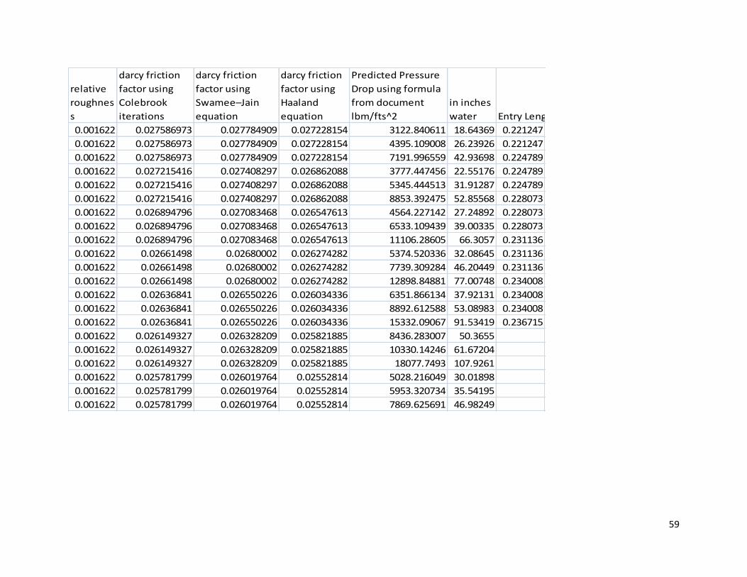
59
relative
roughnes
s
darcy friction
factor using
Colebrook
iterations
darcy friction
factor using
Swamee–Jain
equation
darcy friction
factor using
Haaland
equation
Predicted Pressure
Drop using formula
from document
lbm/fts^2
in inches
water Entry Length
0.001622 0.027586973 0.027784909 0.027228154 3122.840611 18.64369 0.221247
0.001622 0.027586973 0.027784909 0.027228154 4395.109008 26.23926 0.221247
0.001622 0.027586973 0.027784909 0.027228154 7191.996559 42.93698 0.224789
0.001622 0.027215416 0.027408297 0.026862088 3777.447456 22.55176 0.224789
0.001622 0.027215416 0.027408297 0.026862088 5345.444513 31.91287 0.224789
0.001622 0.027215416 0.027408297 0.026862088 8853.392475 52.85568 0.228073
0.001622 0.026894796 0.027083468 0.026547613 4564.227142 27.24892 0.228073
0.001622 0.026894796 0.027083468 0.026547613 6533.109439 39.00335 0.228073
0.001622 0.026894796 0.027083468 0.026547613 11106.28605 66.3057 0.231136
0.001622 0.02661498 0.02680002 0.026274282 5374.520336 32.08645 0.231136
0.001622 0.02661498 0.02680002 0.026274282 7739.309284 46.20449 0.231136
0.001622 0.02661498 0.02680002 0.026274282 12898.84881 77.00748 0.234008
0.001622 0.02636841 0.026550226 0.026034336 6351.866134 37.92131 0.234008
0.001622 0.02636841 0.026550226 0.026034336 8892.612588 53.08983 0.234008
0.001622 0.02636841 0.026550226 0.026034336 15332.09067 91.53419 0.236715
0.001622 0.026149327 0.026328209 0.025821885 8436.283007 50.3655
0.001622 0.026149327 0.026328209 0.025821885 10330.14246 61.67204
0.001622 0.026149327 0.026328209 0.025821885 18077.7493 107.9261
0.001622 0.025781799 0.026019764 0.02552814 5028.216049 30.01898
0.001622 0.025781799 0.026019764 0.02552814 5953.320734 35.54195
0.001622 0.025781799 0.026019764 0.02552814 7869.625691 46.98249
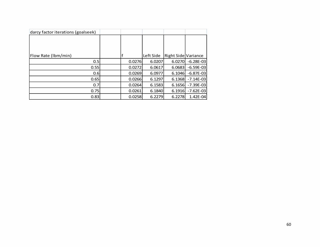
60
darcy factor iterations (goalseek)
Flow Rate (lbm/min) f Left Side Right Side Variance
0.5 0.0276 6.0207 6.0270 -6.28E-03
0.55 0.0272 6.0617 6.0683 -6.59E-03
0.6 0.0269 6.0977 6.1046 -6.87E-03
0.65 0.0266 6.1297 6.1368 -7.14E-03
0.7 0.0264 6.1583 6.1656 -7.39E-03
0.75 0.0261 6.1840 6.1916 -7.62E-03
0.83 0.0258 6.2279 6.2278 1.42E-04
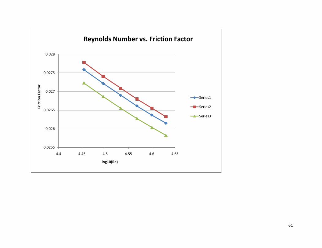
61
0.0255
0.026
0.0265
0.027
0.0275
0.028
4.4 4.45 4.5 4.55 4.6 4.65
Fric
tio
n F
acto
r
log10(Re)
Reynolds Number vs. Friction Factor
Series1
Series2
Series3
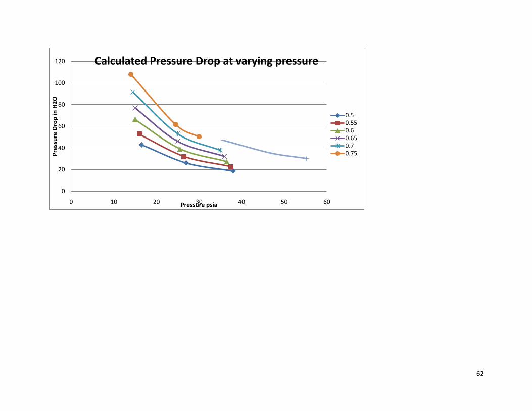
62
0
20
40
60
80
100
120
0 10 20 30 40 50 60
Pre
ssu
re D
rop
in H
2O
Pressure psia
Calculated Pressure Drop at varying pressure
0.50.550.60.650.70.75

63
psia P (psi) P (pa) T (K) R (Pa*m^3/K*mol) MW (g/mol) Density (kg/m^3) Density (lb/ft^3)
38 38 261972 294.26 8.314 28.966 3.101716863 0.193633858
27 27 186138 294.26 8.314 28.966 2.203851456 0.137581952
16.5 16.5 113751 294.26 8.314 28.966 1.346798112 0.084077859
37.5 37.5 258525 294.26 8.314 28.966 3.060904799 0.191086044
26.5 26.5 182691 294.26 8.314 28.966 2.163039392 0.135034138
16 16 110304 294.26 8.314 28.966 1.305986048 0.081530046
36.5 36.5 251631 294.26 8.314 28.966 2.979280671 0.185990416
25.5 25.5 175797 294.26 8.314 28.966 2.081415264 0.12993851
15 15 103410 294.26 8.314 28.966 1.22436192 0.076434418
36 36 248184 294.26 8.314 28.966 2.938468607 0.183442602
25 25 172350 294.26 8.314 28.966 2.0406032 0.127390696
15 15 103410 294.26 8.314 28.966 1.22436192 0.076434418
35 35 241290 294.26 8.314 28.966 2.856844479 0.178346975
25 25 172350 294.26 8.314 28.966 2.0406032 0.127390696
14.5 14.5 99963 294.26 8.314 28.966 1.183549856 0.073886604
30 30 206820 294.26 8.314 28.966 2.44872384 0.152868835
24.5 24.5 168903 294.26 8.314 28.966 1.999791136 0.124842882
14 14 96516 294.26 8.314 28.966 1.142737792 0.07133879
54.7 40 377101.8 294.26 8.314 28.966 4.464839801 0.278730843
46.2 31.5 318502.8 294.26 8.314 28.966 3.771034713 0.235418006
34.95 20.25 240945.3 294.26 8.314 28.966 2.852763273 0.178092193
64
COMSOL Model Report
1. Table of Contents
Title - COMSOL Model Report Table of Contents Model Properties Constants Geometry Geom1 Materials/Coefficients Library Solver Settings Postprocessing Variables
2. Model Properties
Property Value
Model name
Author
Company
Department
Reference
URL
Saved date Apr 26, 2011 4:01:32 PM
Creation date Jan 20, 2011 3:54:48 PM
COMSOL version COMSOL 3.5.0.608
File name: R:\MQP Turbulent quarter inch part 3.mph
Application modes and modules used in this model:
Geom1 (Axial symmetry (2D))

65
o k-ε Turbulence Model (Chemical Engineering Module)
3. Constants
Name Expression Value Description
T 298
P 92514
4. Geometry
Number of geometries: 1
4.1. Geom1
4.1.1. Point mode
4.1.2. Boundary mode
4.1.3. Subdomain mode
5. Geom1
Space dimensions: Axial symmetry (2D)
Independent variables: r, phi, z
5.1. Mesh
5.1.1. Mesh Statistics
Number of degrees of freedom 26200
Number of mesh points 1804
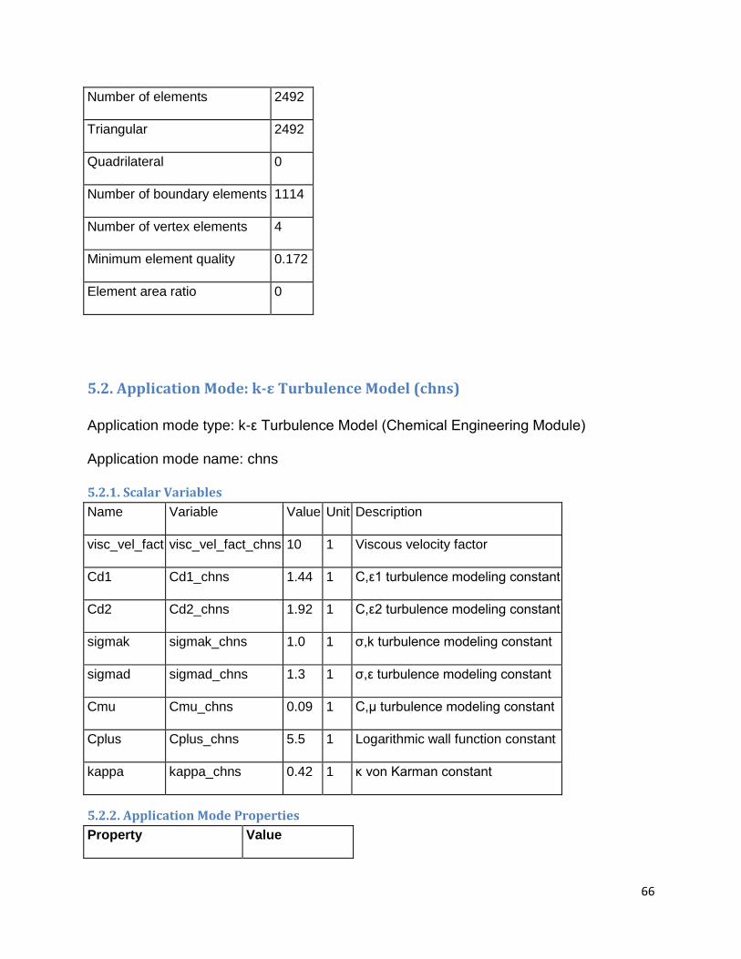
66
Number of elements 2492
Triangular 2492
Quadrilateral 0
Number of boundary elements 1114
Number of vertex elements 4
Minimum element quality 0.172
Element area ratio 0
5.2. Application Mode: k-ε Turbulence Model (chns)
Application mode type: k-ε Turbulence Model (Chemical Engineering Module)
Application mode name: chns
5.2.1. Scalar Variables
Name Variable Value Unit Description
visc_vel_fact visc_vel_fact_chns 10 1 Viscous velocity factor
Cd1 Cd1_chns 1.44 1 C,ε1 turbulence modeling constant
Cd2 Cd2_chns 1.92 1 C,ε2 turbulence modeling constant
sigmak sigmak_chns 1.0 1 σ,k turbulence modeling constant
sigmad sigmad_chns 1.3 1 σ,ε turbulence modeling constant
Cmu Cmu_chns 0.09 1 C,μ turbulence modeling constant
Cplus Cplus_chns 5.5 1 Logarithmic wall function constant
kappa kappa_chns 0.42 1 κ von Karman constant
5.2.2. Application Mode Properties
Property Value

67
Default element type Lagrange - P2 P1
Analysis type Stationary
Corner smoothing Off
Weakly compressible flow On
Turbulence model k-ε
Realizability Off
Non-Newtonian flow Off
Brinkman on by default Off
Two-phase flow Single-phase flow
Swirl velocity Off
Frame Frame (ref)
Weak constraints Off
Constraint type Ideal
5.2.3. Variables
Dependent variables: u, v, w, p, logk, logd, logw, phi, psi, nrw, nzw
Shape functions: shlag(2,'u'), shlag(2,'v'), shlag(1,'p'), shlag(2,'logk'), shlag(2,'logd')
Interior boundaries not active
5.2.4. Boundary Settings
Boundary 1 2 3
Type Symmetry boundary Inlet Outlet
symtype Axial symmetry Symmetry Symmetry
Pressure (p0) Pa 0 0 363272
Normal inflow velocity (U0in) m/s 1 26.87 1
Normal outflow velocity (U0out) m/s 0 0 53

68
Boundary 4
Type Wall
symtype Symmetry
Pressure (p0) Pa 0
Normal inflow velocity (U0in) m/s 1
Normal outflow velocity (U0out) m/s 0
5.2.5. Subdomain Settings
Subdomain 1
Integration order (gporder) 4 4 2 4 4
Constraint order (cporder) 2 2 1 2 2
Density (rho) kg/m3 rho(p[1/Pa],T[1/K])[kg/m^3] (Air)
Dynamic viscosity (eta) Pa⋅s eta(T[1/K])[Pa*s] (Air)
Surface tension coefficient (sigma) N/m 0[S/m] (Air)
Reinitialization parameter (gamma) m/s 1.4 (Air)
Subdomain initial value 1
Logarithm of turbulent kinetic energy (logk) 1 101325
6. Materials/Coefficients Library
6.1. Air
Parameter Value
Heat capacity at constant pressure (C) Cp(T[1/K])[J/(kg*K)]
Speed of sound (cs) cs(T[1/K])[m/s]
Dynamic viscosity (eta) eta(T[1/K])[Pa*s]
Ratio of specific heats (gamma) 1.4

69
Thermal conductivity (k) k(T[1/K])[W/(m*K)]
Kinematic viscosity (nu0) nu0(T[1/K])[m^2/s]
Density (rho) rho(p[1/Pa],T[1/K])[kg/m^3]
Electric conductivity (sigma) 0[S/m]
6.1.1. Functions
Function Expression Derivatives Complex output
cs(T) sqrt(1.4*287*T) d(sqrt(1.4*287*T),T) false
rho(p,T) p*0.02897/8.314/T d(p*0.02897/8.314/T,p), d(p*0.02897/8.314/T,T) false
6.1.2. Piecewise Analytic Functions
6.1.2.1. Function: Cp(T)
Type: Polynomial
xstart xend f(x)
200 1600 0 1.04763657E+03 1 -3.72589265E-01 2 9.45304214E-04 3 -6.02409443E-07 4
1.28589610E-10
6.1.2.2. Function: eta(T)
Type: Polynomial
xstart xend f(x)
200 1600 0 -8.38278000E-07 1 8.35717342E-08 2 -7.69429583E-11 3 4.64372660E-14 4 -
1.06585607E-17
6.1.2.3. Function: nu0(T)
Type: Polynomial
xstart xend f(x)
200 1600 0 -5.86912450E-06 1 5.01274491E-08 2 7.50108343E-11 3 1.80336823E-15 4 -
2.91688030E-18

70
6.1.2.4. Function: k(T)
Type: Polynomial
xstart xend f(x)
200 1600 0 -2.27583562E-03 1 1.15480022E-04 2 -7.90252856E-08 3 4.11702505E-11 4 -
7.43864331E-15
7. Solver Settings
Solve using a script: off
Analysis type Stationary
Auto select solver On
Solver Stationary segregated
Solution form Automatic
Symmetric Off
Adaptive mesh refinement Off
Optimization/Sensitivity Off
Plot while solving Off
7.1. Segregated Groups
7.1.1. Group 1
Parameter Value
Components u v p
Tolerance 1e-3
7.1.1.1. Direct (PARDISO)
Solver type: Linear system solver
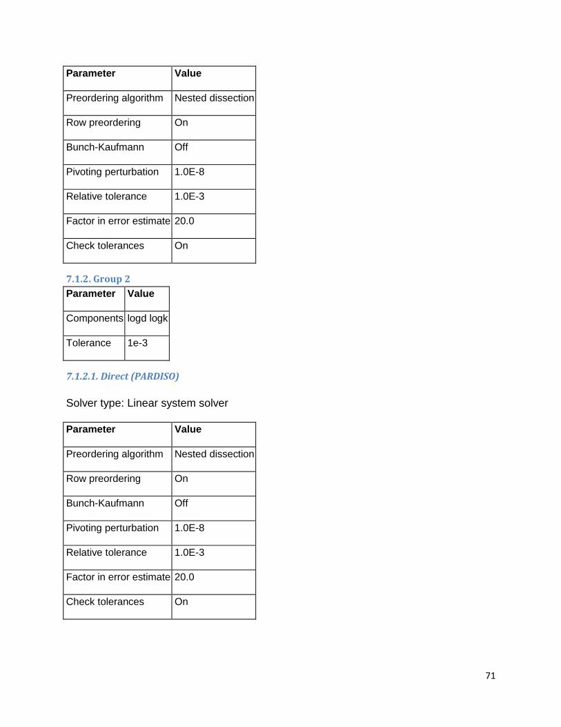
71
Parameter Value
Preordering algorithm Nested dissection
Row preordering On
Bunch-Kaufmann Off
Pivoting perturbation 1.0E-8
Relative tolerance 1.0E-3
Factor in error estimate 20.0
Check tolerances On
7.1.2. Group 2
Parameter Value
Components logd logk
Tolerance 1e-3
7.1.2.1. Direct (PARDISO)
Solver type: Linear system solver
Parameter Value
Preordering algorithm Nested dissection
Row preordering On
Bunch-Kaufmann Off
Pivoting perturbation 1.0E-8
Relative tolerance 1.0E-3
Factor in error estimate 20.0
Check tolerances On

72
7.2. Segregated Scheme
7.2.1. Step 1
Parameter Value
Segregated group 1
Termination technique Iteration
Damping constant 0.5
Number of iterations 1
Maximum number of iterations 20
Tolerance 1.0E-2
Damping technique Constant
Initial damping factor 1.0
Minimum damping factor 1.0E-4
Restriction for step size update 10.0
7.2.2. Step 2
Parameter Value
Segregated group 2
Termination technique Iteration
Damping constant 0.5
Number of iterations 3
Maximum number of iterations 20
Tolerance 1.0E-2
Damping technique Constant
Initial damping factor 1.0
Minimum damping factor 1.0E-4

73
Restriction for step size update 10.0
7.3. Stationary
Parameter Value
Linearity Automatic
Maximum number of segregated iterations 100
7.4. Advanced
Parameter Value
Constraint handling method Elimination
Null-space function Automatic
Automatic assembly block size On
Assembly block size 1000
Use Hermitian transpose of constraint matrix and in symmetry detection Off
Use complex functions with real input Off
Stop if error due to undefined operation On
Store solution on file Off
Type of scaling None
Manual scaling
Row equilibration On
Manual control of reassembly Off
Load constant On
Constraint constant On
Mass constant On
Damping (mass) constant On
Jacobian constant On

74
Constraint Jacobian constant On
8. Postprocessing
9. Variables
9.1. Boundary
Name Description Unit Expression
K_r_chns Viscous force per
area, r component
Pa (eta_chns+etaT_chns) * (nr_chns * (2 * ur-2 *
divU_chns/3)+nz_chns * (uz+vr))
T_r_chns Total force per area,
r component
Pa -nr_chns * p+nr_chns * (eta_chns+etaT_chns) * (2 * ur-2
* divU_chns/3)+nz_chns * (eta_chns+etaT_chns) *
(uz+vr)
K_z_chns Viscous force per
area, z component
Pa (eta_chns+etaT_chns) * (nr_chns * (vr+uz)+nz_chns * (2
* vz-2 * divU_chns/3))
T_z_chns Total force per area,
z component
Pa -nz_chns * p+nr_chns * (eta_chns+etaT_chns) *
(vr+uz)+nz_chns * (eta_chns+etaT_chns) * (2 * vz-2 *
divU_chns/3)
9.2. Subdomain
Name Description Unit Expression
U_chns Velocity field m/s sqrt(u^2+v^2)
V_chns Vorticity 1/s uz-vr
divU_chns Divergence of
velocity field
1/s ur+vz+u/r
Dlogd_chns Effective
turbulence
diffusion
coefficient for
logd
Pa*s etaT_chns/sigmad_chns+eta_chns

75
Slogd_chns Source term for
logd
kg/(m^3*s) Cd1_chns * (etaT_chns * exp(-logk) * pT_chns-2 *
rho_chns * divU_chns/3)-Cd2_chns * rho_chns *
exp(logd-nojac(logk))
d0_chns Turbulent
dissipation rate
m^2/s^3 exp(logd)
etaT_chns Turbulent
viscosity
Pa*s nojac(rho_chns * Cmu_chns * exp(2 * logk-logd))
pT_chns Turbulent
energy
production
1/s^2 2 * ur^2+2 * vz^2+(uz+vr)^2+2 * u^2/r^2-2 *
divU_chns^2/3
k0_chns Turbulent
kinetic energy
m^2/s^2 exp(logk)
Dlogk_chns Effective
turbulence
diffusion
coefficient for
logk
Pa*s etaT_chns/sigmak_chns+eta_chns
Slogk_chns Source term for
logk
kg/(m^3*s) etaT_chns * exp(-logk) * pT_chns-2 * rho_chns *
divU_chns/3-rho_chns * exp(logd-nojac(logk))
res_logk_chns Equation
residual for
logk
kg/(m^2*s) -Dlogk_chns * (r * logkrr+r * logkzz+logkr)-r * (-
rho_chns * (u * logkr+v * logkz)+Dlogk_chns *
(logkr^2+logkz^2)+Slogk_chns)
res_logd_chns Equation
residual for
logd
kg/(m^2*s) -Dlogd_chns * (r * logdrr+r * logdzz+logdr)-r * (-
rho_chns * (u * logdr+v * logdz)+Dlogd_chns *
(logdr^2+logdz^2)+Slogd_chns)
cellRe_chns Cell Reynolds
number
1 rho_chns * U_chns * h/eta_chns
res_u_chns Equation
residual for u
Pa r * (rho_chns * (u * ur+v * uz)+pr-F_r_chns)+2 *
(eta_chns+etaT_chns) * (u/r-ur)-
(eta_chns+etaT_chns) * r * (2 * urr+uzz+vrz)+2 *
(eta_chns+etaT_chns) * (r * urr+r * vzr+ur-u/r)/3+2 *
r * d(rho_chns * exp(logk),r)/3
res_v_chns Equation
residual for v
Pa r * (rho_chns * (u * vr+v * vz)+pz-F_z_chns)-
(eta_chns+etaT_chns) * (r * (vrr+uzr)+2 * r *
vzz+uz+vr)+2 * (eta_chns+etaT_chns) * (r * urz+r *

76
vzz+uz)/3+2 * r * d(rho_chns * exp(logk),z)/3
beta_r_chns Convective
field, r
component
Pa*s r * rho_chns * u
beta_z_chns Convective
field, z
component
Pa*s r * rho_chns * v
Dm_chns Mean diffusion
coefficient
kg/s r * (eta_chns+etaT_chns)
da_chns Total time scale
factor
kg/m^2 r * rho_chns
taum_chns GLS time-scale m^3*s/kg nojac(1/max(2 * rho_chns * sqrt(emetric(u,v)),48 *
(eta_chns+etaT_chns)/h^2))
tauc_chns GLS time-scale m^2/s 0.5 * nojac(if(u^2+v^2< U_ref_chns,(u^2+v^2) *>
res_p_chns Equation
residual for p
kg/(m^2*s) r * (rho_chns * divU_chns+d(rho_chns,r) *
u+d(rho_chns,z) * v)
tau_logk_chns GLS time-scale m^3*s/kg nojac(0.5 * h/max(rho_chns * U_chns,6 *
Dlogk_chns/h))
tau_logd_chns GLS time-scale m^3*s/kg nojac(0.5 * h/max(rho_chns * U_chns,6 *
Dlogd_chns/h))