compton polarimetry at jefferson lab · dave gaskell jefferson lab intersections between nuclear...
TRANSCRIPT
1
Compton Polarimetry at Jefferson Lab
Dave GaskellJefferson Lab
Intersections Between Nuclear Physics and Quantum InformationMarch 28-30, 2018
1. Compton scattering for electron beam polarimetry2. Compton polarimetry at Jefferson Lab
à Techniques and apparatusà Precisionà Application for nuclear physics experiments
2
Polarized Electrons at Jefferson Lab• Polarized electron beam at JLab has enabled a large program of
measurements aimed at understanding hadronic structure– Proton elastic form factors via recoil proton polarization– Double-spin asymmetries with polarized proton, deuteron and
3He targets à polarized quark PDFs– Parity violating electron scattering to probe strange quarks in
nucleon• Most experiments of the above type require only modest precision in
knowledge of beam polarization (dP/P~2-3%)• More recently, PVES experiments have been used to probe for new
physics beyond the Standard Model – for such experiments, beam polarization becomes one of the limiting systematics– Q-Weak (elastic ep) à dP/P < 1%– MOLLER (elastic ee) à dP/P < 0.5%– SOLID (PVDIS) à dP/P ~0.4% Future
3
JLab Accelerator and Polarimeters
A B C
D
Injector
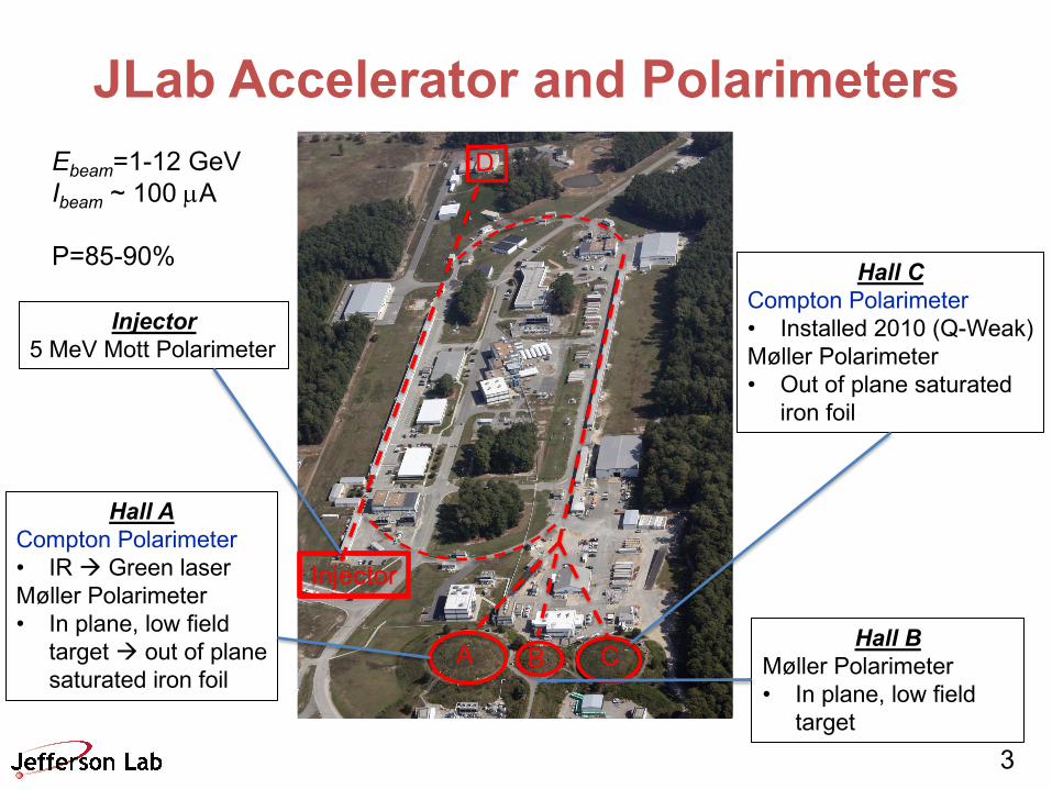
Injector5 MeV Mott Polarimeter
Hall ACompton Polarimeter• IR à Green laserMøller Polarimeter• In plane, low field
target à out of plane saturated iron foil
Hall CCompton Polarimeter• Installed 2010 (Q-Weak)Møller Polarimeter• Out of plane saturated
iron foil
Hall BMøller Polarimeter• In plane, low field
target
Ebeam=1-12 GeVIbeam ~ 100 µA
P=85-90%
4
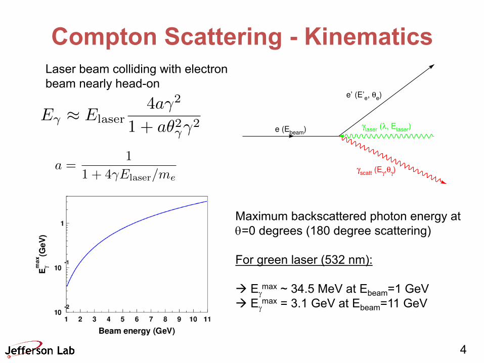
Compton Scattering - Kinematics
e (Ebeam)
γscatt (Eγ,θγ)
γlaser (λ, Elaser)
e’ (E’e, θe)
E� ⇡ Elaser4a�2
1 + a✓2��2
a =1
1 + 4�Elaser/me
Maximum backscattered photon energy atq=0 degrees (180 degree scattering)
For green laser (532 nm):
à Egmax ~ 34.5 MeV at Ebeam=1 GeV
à Egmax = 3.1 GeV at Ebeam=11 GeV
Laser beam colliding with electron beam nearly head-on
5
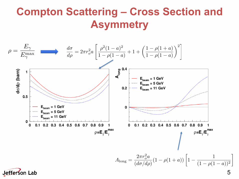
Compton Scattering – Cross Section and Asymmetry
d�
d⇢= 2⇡r2oa
"⇢2(1� a)2
1� ⇢(1� a)+ 1 +
✓1� ⇢(1 + a)
1� ⇢(1� a)
◆2#
⇢ =E�
Emax�
Along =2⇡r2oa
(d�/d⇢)(1� ⇢(1 + a))
1� 1
(1� ⇢(1� a))2
�
6
Compton Polarimetry at JLab• Compton polarimetry routinely used at colliders/storage rings
before use at JLab
• Several challenges for use at JLab
– Low beam currents (~100 µA) compared to colliders
• Measurements can take on the order of hours
• Makes systematic studies difficult
– At lower energies, relatively small asymmetries
• Smaller asymmetries lead to harder-to-control systematics
• Strong dependence of asymmetry on Eg leads to non-trivial determination of analyzing power
– Understanding the detector response crucial

7
JLab Compton PolarimetersHall A and C have similar (although not identical) Compton polarimeters
Components:
1. 4-dipole chicane: Deflect electron beam vertically
• 6 GeV configuration: Hall A à 30 cm, Hall C à 57 cm
• 12 GeV configuration: Hall A à 21.5 cm, Hall C à 13 cm
2. Laser system: Fabry-Pérot cavity pumped by CW laser resulting in few kW of
stored laser power
3. Photon detector: PbWO4 or GSO – operated in integrating mode
4. Electron detector: segmented strip detector
8
Fabry-Pérot Cavity• Compton polarimeter measurement time a challenge at JLab
– Example: At 1 GeV and 180 µA, a 1% (statistics) measurement with 10 W CW laser would take on the order of 1 day!
– Not much to be gained with pulsed lasers given JLab beam structure (nearly CW)
• A high-finesse (high-gain) Fabry-Pérot cavity locked to narrow linewidth laser is capable of storing several kW of CW laser power– First proposed for use at JLab in mid-90’s, implemented in Hall A
in late 90’s (Hall C in 2010, HERA..)
• Requires routing electron beam through center of cavity– Radiation damage to mirrors an early concern– Need non-zero crossing angle between laser and beam à some
reduction in FOM
9
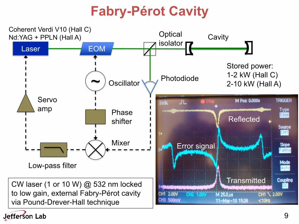
Fabry-Pérot Cavity
Laser EOMCavity
~ Oscillator
Phaseshifter
Mixer
Low-pass filter
Servoamp
Opticalisolator
Photodiode
Error signal
Transmitted
Reflected
Coherent Verdi V10 (Hall C)Nd:YAG + PPLN (Hall A)
CW laser (1 or 10 W) @ 532 nm locked to low gain, external Fabry-Pérot cavity via Pound-Drever-Hall technique
Stored power:1-2 kW (Hall C)2-10 kW (Hall A)
10
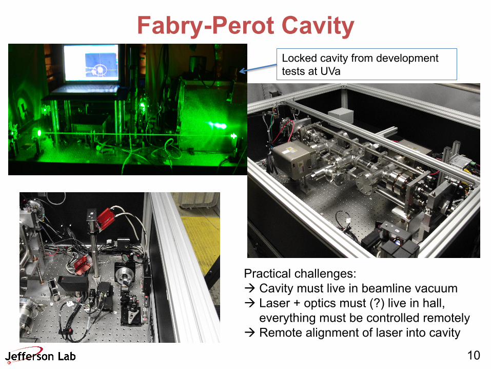
Fabry-Perot CavityLocked cavity from development tests at UVa
Reflected
Transmitted
Error signal
Practical challenges:à Cavity must live in beamline vacuumà Laser + optics must (?) live in hall,
everything must be controlled remotelyà Remote alignment of laser into cavity
11
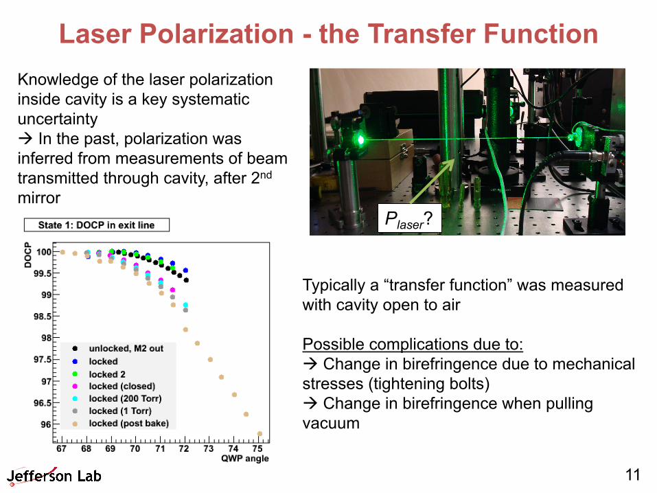
Laser Polarization - the Transfer FunctionKnowledge of the laser polarization inside cavity is a key systematic uncertaintyà In the past, polarization was inferred from measurements of beam transmitted through cavity, after 2nd
mirrorPlaser?
Typically a “transfer function” was measured with cavity open to air
Possible complications due to:à Change in birefringence due to mechanical stresses (tightening bolts)à Change in birefringence when pulling vacuum
12
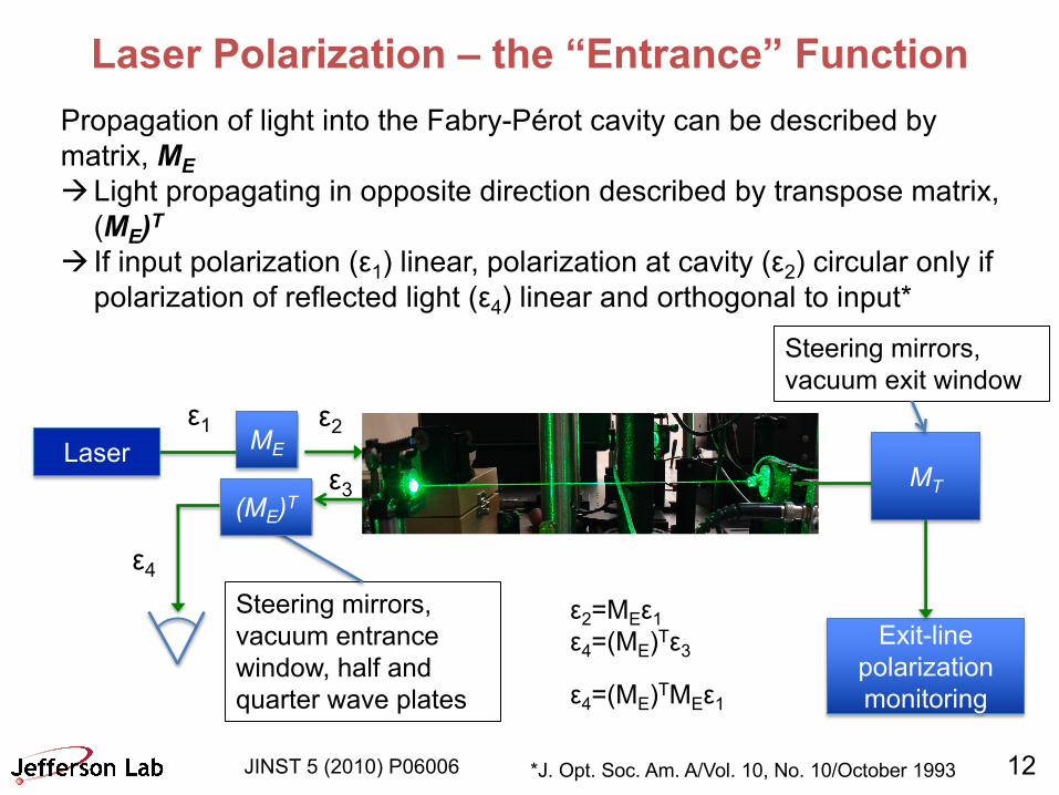
Laser Polarization – the “Entrance” FunctionPropagation of light into the Fabry-Pérot cavity can be described by
matrix, MEàLight propagating in opposite direction described by transpose matrix,
(ME)Tà If input polarization (ε
1) linear, polarization at cavity (ε
2) circular only if
polarization of reflected light (ε4) linear and orthogonal to input*
LaserME
MT
Exit-line
polarization
monitoring
Steering mirrors,
vacuum entrance
window, half and
quarter wave plates
(ME)T
Steering mirrors,
vacuum exit window
ε1 ε
2
ε3
ε4
ε2=M
Eε
1
ε4=(M
E)Tε
3
ε4=(M
E)TM
Eε
1
*J. Opt. Soc. Am. A/Vol. 10, No. 10/October 1993JINST 5 (2010) P06006
13
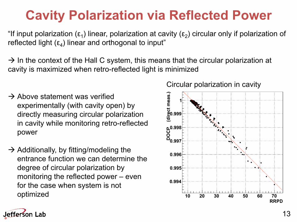
Cavity Polarization via Reflected Power“If input polarization (ε1) linear, polarization at cavity (ε2) circular only if polarization of reflected light (ε4) linear and orthogonal to input”
à In the context of the Hall C system, this means that the circular polarization at cavity is maximized when retro-reflected light is minimized
Circular polarization in cavityà Above statement was verified
experimentally (with cavity open) by directly measuring circular polarization in cavity while monitoring retro-reflected power
à Additionally, by fitting/modeling the entrance function we can determine the degree of circular polarization by monitoring the reflected power – even for the case when system is not optimized
14
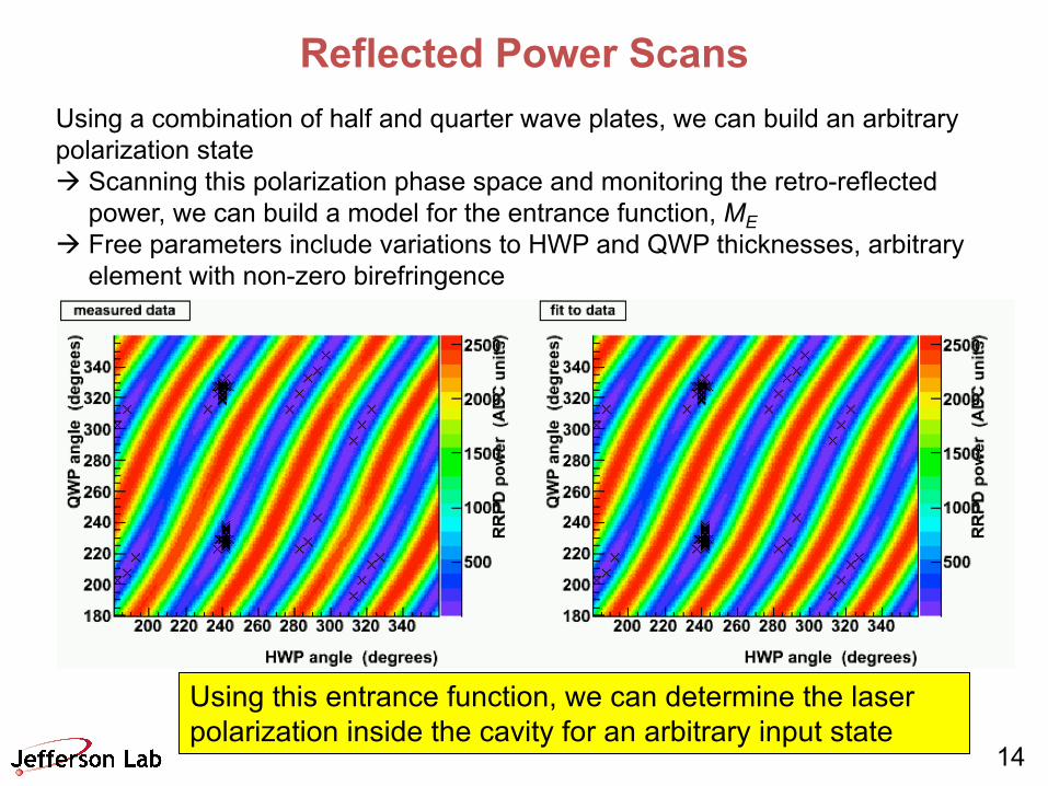
Reflected Power ScansUsing a combination of half and quarter wave plates, we can build an arbitrary polarization stateà Scanning this polarization phase space and monitoring the retro-reflected
power, we can build a model for the entrance function, MEà Free parameters include variations to HWP and QWP thicknesses, arbitrary
element with non-zero birefringence
Using this entrance function, we can determine the laser polarization inside the cavity for an arbitrary input state
15
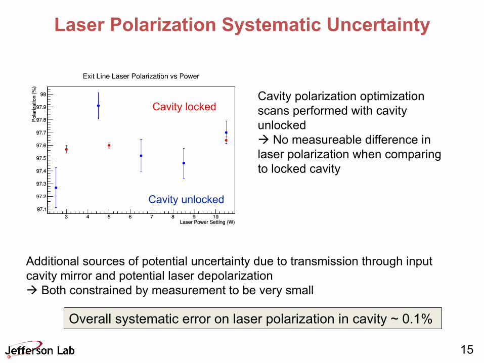
Laser Polarization Systematic Uncertainty
Cavity polarization optimization scans performed with cavity unlockedà No measureable difference in laser polarization when comparing to locked cavity
Cavity locked
Cavity unlocked
Additional sources of potential uncertainty due to transmission through input cavity mirror and potential laser depolarizationà Both constrained by measurement to be very small
Overall systematic error on laser polarization in cavity ~ 0.1%
16
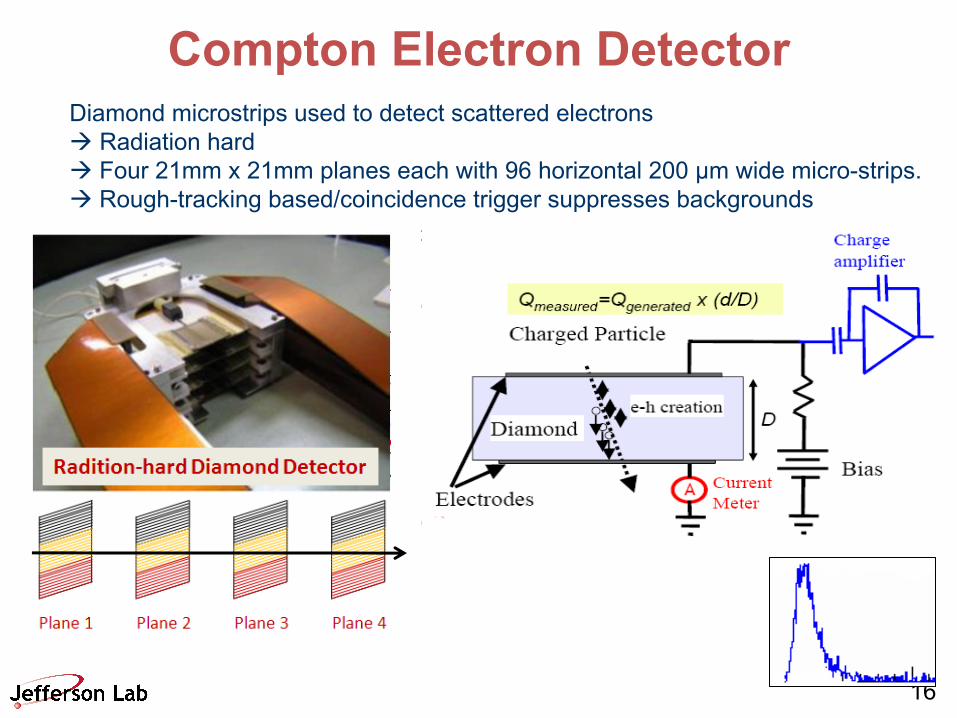
Compton Electron DetectorDiamond microstrips used to detect scattered electronsà Radiation hardà Four 21mm x 21mm planes each with 96 horizontal 200 μm wide micro-strips.à Rough-tracking based/coincidence trigger suppresses backgrounds
17
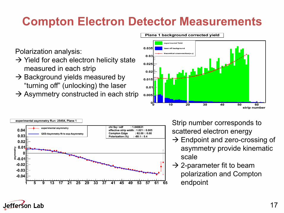
Compton Electron Detector Measurements
Polarization analysis:à Yield for each electron helicity state
measured in each stripà Background yields measured by
“turning off” (unlocking) the laserà Asymmetry constructed in each strip
Strip number corresponds to scattered electron energyà Endpoint and zero-crossing of
asymmetry provide kinematic scale
à 2-parameter fit to beam polarization and Compton endpoint
18
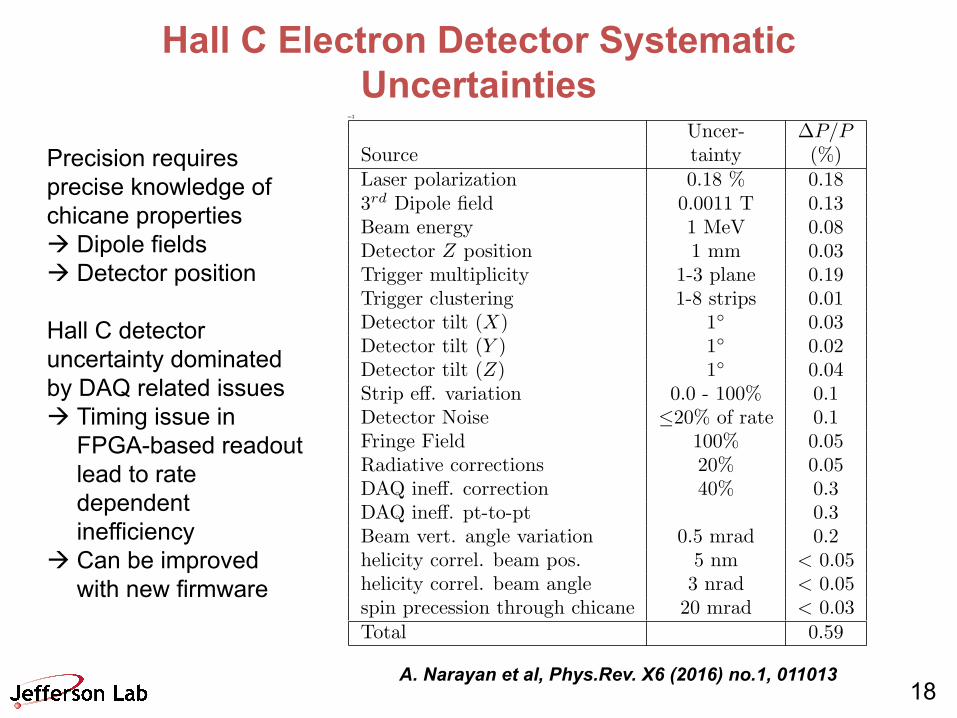
Hall C Electron Detector Systematic Uncertainties
=3
Uncer- �P/PSource tainty (%)Laser polarization 0.18 % 0.183rd Dipole field 0.0011 T 0.13Beam energy 1 MeV 0.08Detector Z position 1 mm 0.03Trigger multiplicity 1-3 plane 0.19Trigger clustering 1-8 strips 0.01Detector tilt (X) 1� 0.03Detector tilt (Y ) 1� 0.02Detector tilt (Z) 1� 0.04Strip e�. variation 0.0 - 100% 0.1Detector Noise �20% of rate 0.1Fringe Field 100% 0.05Radiative corrections 20% 0.05DAQ ine�. correction 40% 0.3DAQ ine�. pt-to-pt 0.3Beam vert. angle variation 0.5 mrad 0.2helicity correl. beam pos. 5 nm < 0.05helicity correl. beam angle 3 nrad < 0.05spin precession through chicane 20 mrad < 0.03Total 0.59
A. Narayan et al, Phys.Rev. X6 (2016) no.1, 011013
Precision requires precise knowledge of chicane propertiesà Dipole fieldsà Detector position
Hall C detector uncertainty dominated by DAQ related issuesà Timing issue in
FPGA-based readout lead to rate dependent inefficiency
à Can be improved with new firmware
19
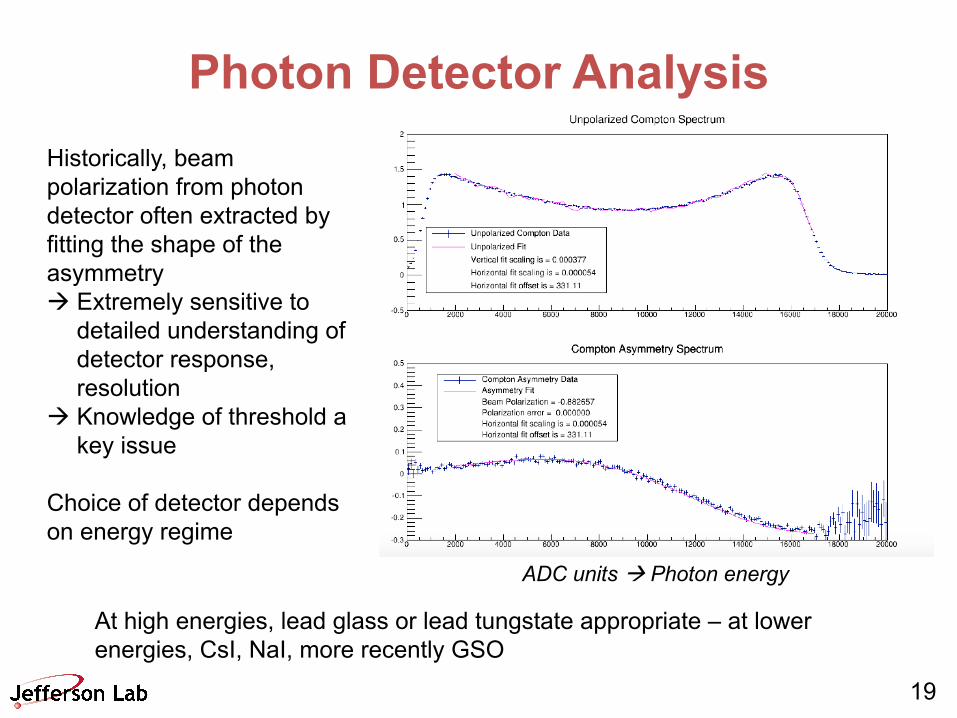
Photon Detector AnalysisHistorically, beam polarization from photon detector often extracted by fitting the shape of the asymmetryà Extremely sensitive to
detailed understanding of detector response, resolution
à Knowledge of threshold a key issue
Choice of detector depends on energy regime
At high energies, lead glass or lead tungstate appropriate – at lower energies, CsI, NaI, more recently GSO
ADC units à Photon energy

20
Hall A Compton – Photon Detector Upgrade
( )dEEAPPEdEdEELTE
E
leò ±=± max
0)(1)()( g
se -+
-+
+-
=EEEE
AExp
Uncertainties can be significantly reduced using energy weighted asymmetry
à No threshold, so analyzing power well understoodà Less sensitive to understanding detector resolutionà Understanding detector non-linearity over relevant range of signal size most
significant challenge à LED pulser system
Poor Linearity Good Linearity
New detector (GSO) for low energy – new technique
Spearheaded by Carnegie Mellon U.
Gregg Franklin – EIC14
21
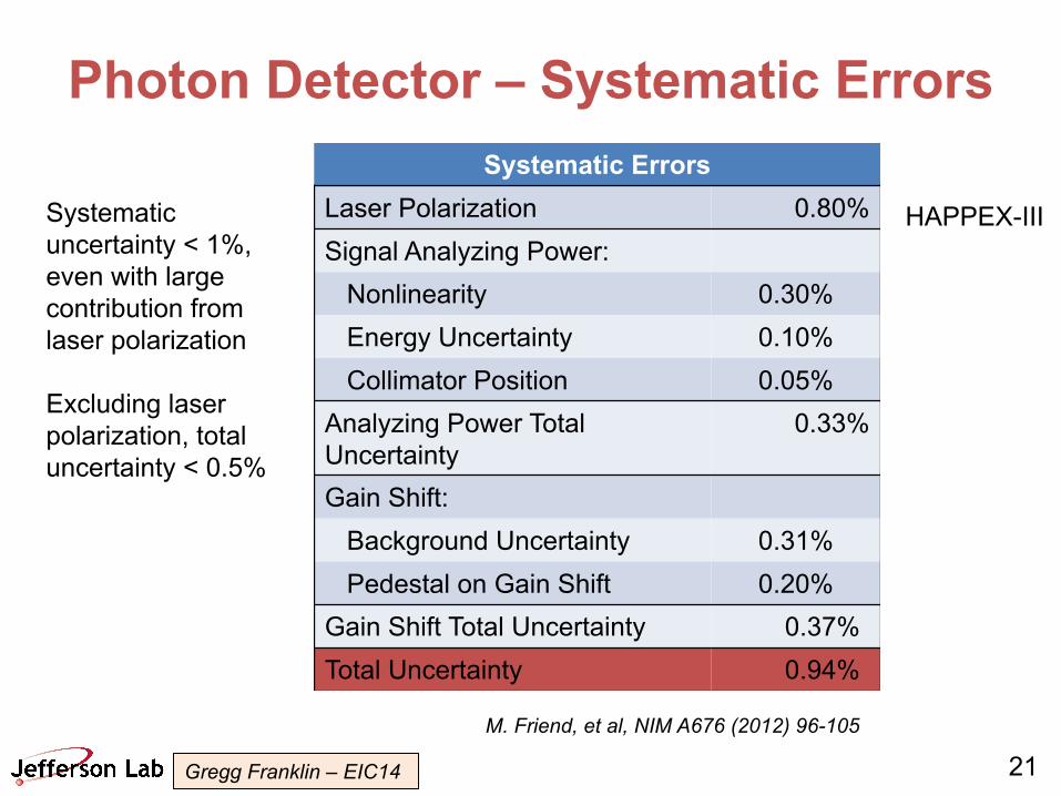
Photon Detector – Systematic ErrorsSystematic Errors
Laser Polarization 0.80%
Signal Analyzing Power:
Nonlinearity 0.30%
Energy Uncertainty 0.10%
Collimator Position 0.05%
Analyzing Power Total
Uncertainty
0.33%
Gain Shift:
Background Uncertainty 0.31%
Pedestal on Gain Shift 0.20%
Gain Shift Total Uncertainty 0.37%
Total Uncertainty 0.94%
M. Friend, et al, NIM A676 (2012) 96-105
HAPPEX-IIISystematic
uncertainty < 1%,
even with large
contribution from
laser polarization
Excluding laser
polarization, total
uncertainty < 0.5%
Gregg Franklin – EIC14
22
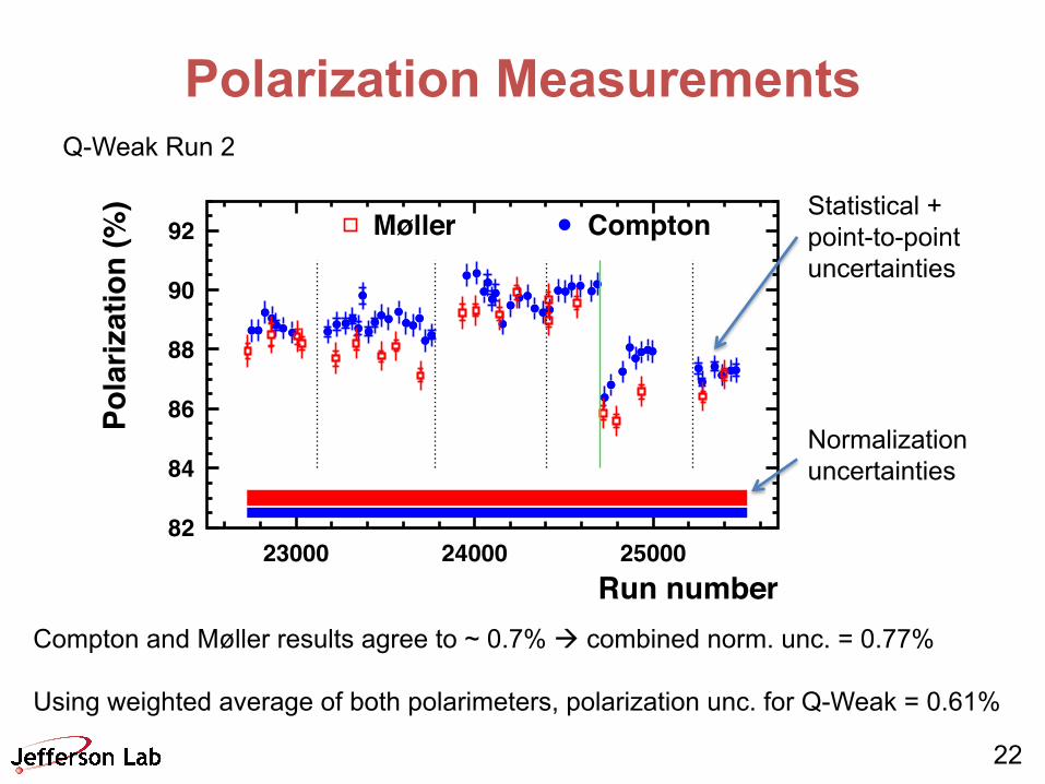
Polarization Measurements
82
84
86
88
90
92
23000 24000 25000Run number
Pola
rizat
ion
(%)
ComptonMøller
Q-Weak Run 2
Compton and Møller results agree to ~ 0.7% à combined norm. unc. = 0.77%
Using weighted average of both polarimeters, polarization unc. for Q-Weak = 0.61%
Statistical + point-to-point uncertainties
Normalization uncertainties
23
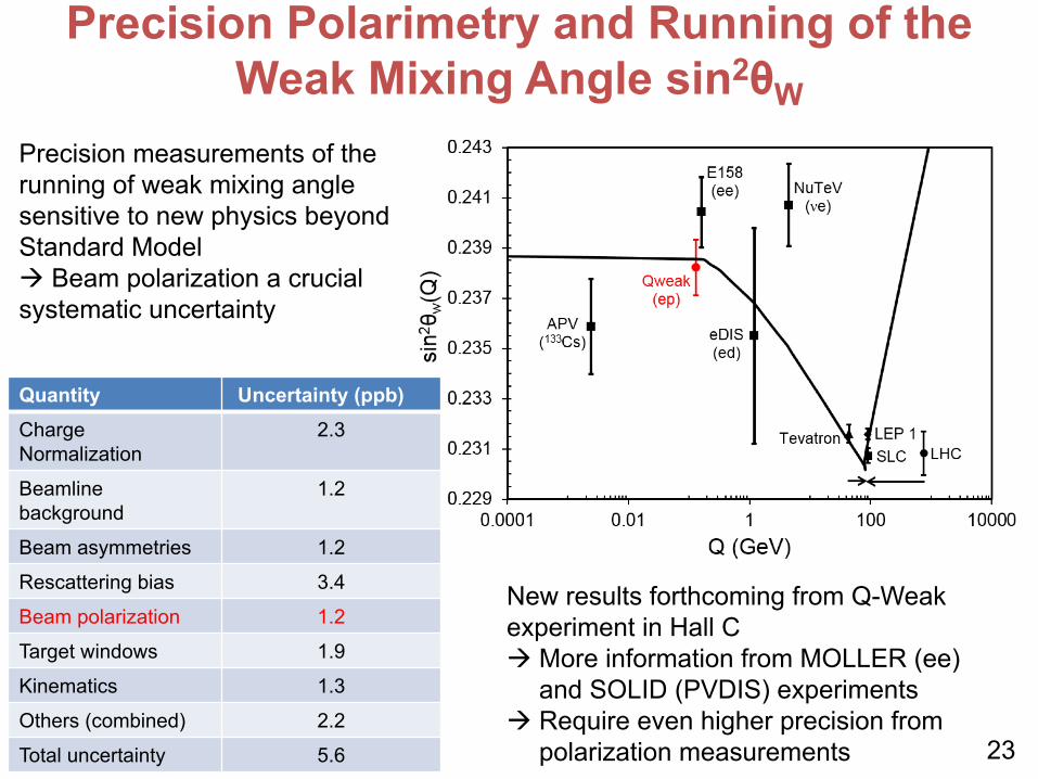
Precision Polarimetry and Running of the Weak Mixing Angle sin2θW
Quantity Uncertainty (ppb)Charge Normalization
2.3
Beamline background
1.2
Beam asymmetries 1.2
Rescattering bias 3.4
Beam polarization 1.2
Target windows 1.9
Kinematics 1.3
Others (combined) 2.2
Total uncertainty 5.6
Precision measurements of the running of weak mixing angle sensitive to new physics beyond Standard Modelà Beam polarization a crucial systematic uncertainty
New results forthcoming from Q-Weak experiment in Hall Cà More information from MOLLER (ee)
and SOLID (PVDIS) experimentsà Require even higher precision from
polarization measurements

24
Compton Polarimetry at JLEIC
• Work is underway to develop a Compton polarimeter design for use at a future electron-ion collider à desired precision on the order of 1%
• JLEIC electron beam parameters: 3-10 GeV, 476 MHz, beam currents of order ~1 A• Design based on successful JLab Hall A and Hall C polarimeters
• Focusing on electron detection for now• Some desire to measure polarization of each bunch individually- this would require
• RF pulsed laser system• Fast electron detector
• Simultaneous sensitivity to transverse beam polarization would be a bonus
gc
Laser System
e- beam from IP
Low-Q2 tagger for low-energy electrons
Electrontracking detector
Photon Calorimeter
gB
Luminosity Monitor
25
Summary• Compton polarimetry an important tool for nuclear physics
experiments at JLab – Highest precision generally required by PVES program
• Relatively low currents, CW beam at JLab required novel laser solution– Laser coupled to moderate/high gain FP cavity– Knowledge of laser polarization in cavity was a challenge in the
past à no longer significant source of uncertainty• Electron and photon detection provide quasi-independent
measurements of polarization with different systematic uncertainties– Choice of detector technology driven by beam energy,
polarimeter properties, expected integrated luminosity• Application at future EIC may provide new technical challenges
– High currents provide high rates, but large backgrounds as well

26
EXTRA
27
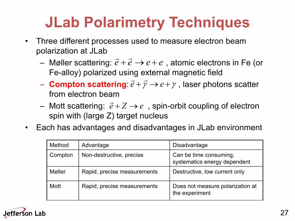
JLab Polarimetry Techniques• Three different processes used to measure electron beam
polarization at JLab– Møller scattering: , atomic electrons in Fe (or
Fe-alloy) polarized using external magnetic field– Compton scattering: , laser photons scatter
from electron beam– Mott scattering: , spin-orbit coupling of electron
spin with (large Z) target nucleus• Each has advantages and disadvantages in JLab environment
eeee +®+!!
gg +®+ ee !!
eZe ®+!
Method Advantage Disadvantage
Compton Non-destructive, precise Can be time consuming, systematics energy dependent
Møller Rapid, precise measurements Destructive, low current only
Mott Rapid, precise measurements Does not measure polarization at the experiment
28
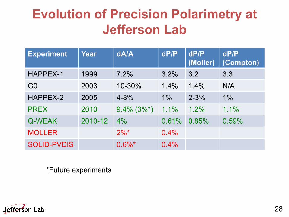
Evolution of Precision Polarimetry at Jefferson Lab
Experiment Year dA/A dP/P dP/P (Moller)
dP/P (Compton)
HAPPEX-1 1999 7.2% 3.2% 3.2 3.3
G0 2003 10-30% 1.4% 1.4% N/A
HAPPEX-2 2005 4-8% 1% 2-3% 1%
PREX 2010 9.4% (3%*) 1.1% 1.2% 1.1%
Q-WEAK 2010-12 4% 0.61% 0.85% 0.59%
MOLLER 2%* 0.4%
SOLID-PVDIS 0.6%* 0.4%
*Future experiments

29
Møller-Compton Cross CalibrationMøller measurements typically made at 1 μA, Compton measurements at 180 μA
à Performed a direct comparison at the same beam current à 4.5 μA
à Møller analysis required extra corrections for beam heating, dead time
à Compton analysis slightly more sensitive to noise at lower current
82
84
86
88
90
92
Pola
rizat
ion
(%) Compton 4.5 µA
Compton 180 µAMøller 4.5 µA
85
86
87
88
89
25280 25300 25320 25340Run number
86.92 +/- 0.47%
86.54 +/- 0.72%87.44 +/- 0.84% 87.16 +/- 0.53%
30
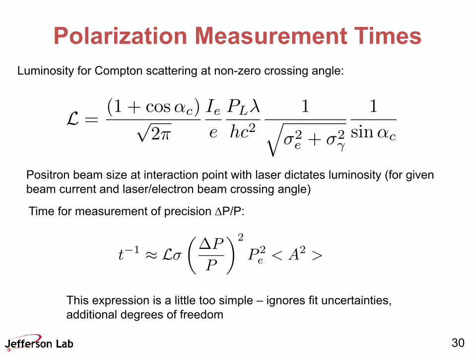
Polarization Measurement TimesLuminosity for Compton scattering at non-zero crossing angle:
L =(1 + cos↵c)p
2⇡
Iee
PL�
hc21q
�2e + �2
�
1
sin↵c
Positron beam size at interaction point with laser dictates luminosity (for given beam current and laser/electron beam crossing angle)
Time for measurement of precision DP/P:
t�1 ⇡ L�✓�P
P
◆2
P 2e < A2 >
This expression is a little too simple – ignores fit uncertainties, additional degrees of freedom
31
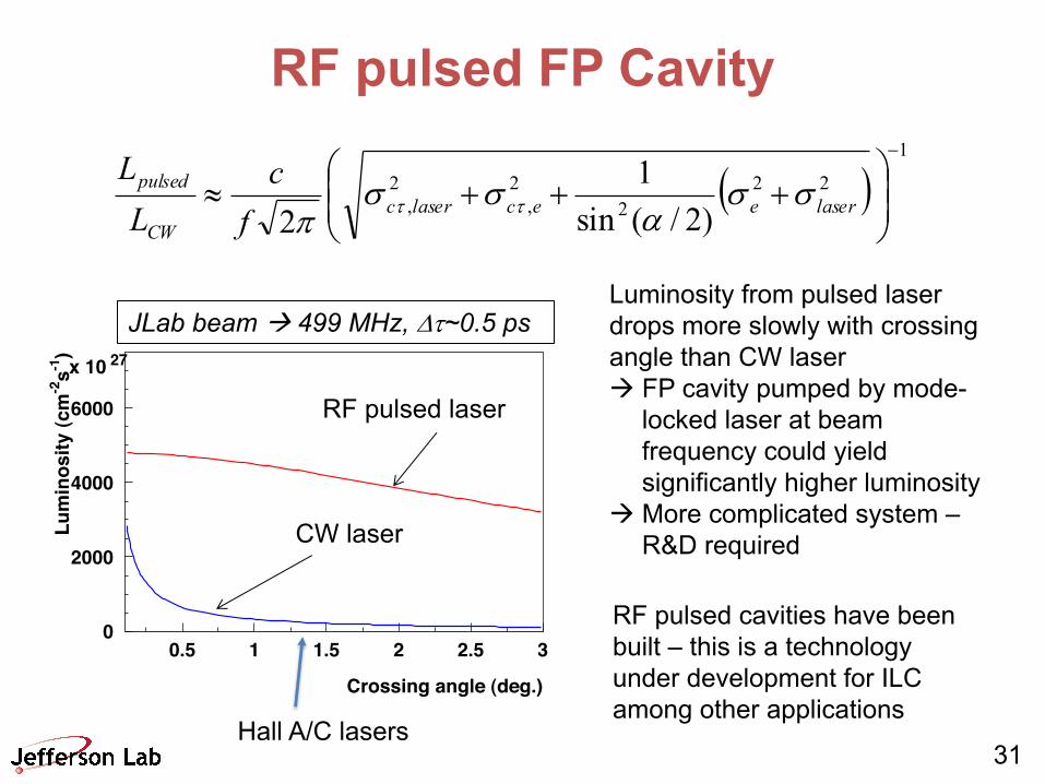
RF pulsed FP Cavity
Crossing angle (deg.)
Lu
min
osit
y (
cm
-2s
-1)
0
2000
4000
6000
x 10 27
0.5 1 1.5 2 2.5 3
RF pulsed laser
CW laser
RF pulsed cavities have been built – this is a technology under development for ILC among other applications
JLab beam à 499 MHz, Dt~0.5 ps
( )1
222
2,
2, )2/(sin
12
-
÷÷ø
öççè
æ+++» lasereeclaserc
CW
pulsed
fc
LL
ssa
ssp tt
Luminosity from pulsed laser drops more slowly with crossing angle than CW laserà FP cavity pumped by mode-
locked laser at beam frequency could yield significantly higher luminosity
à More complicated system –R&D required
Hall A/C lasers