Computation of NACA0012 Airfoil Transonic Buffet

Phenomenon with Unsteady Navier-Stokes Equations

Juntao Xiong ∗, Feng Liu † Shijun Luo ‡,

University of California Irvine, Irvine, CA, 92697, USA

A computational study of transonic buffet phenomenon over NACA0012 airfoil is pre-

sented using unsteady Reynolds-averaged Navier-Stokes Equations. Computations are con-

ducted at freestream Mach numbers from 0.82 to 0.89 at zero angle of attack for Reynolds

numbers of 3.0 and 10.0 million with transition fixed at 5% chord length. Numerical simu-

lation reveals the transonic buffet occurs in a narrow range of freestream Mach numbers of

0.85-0.87. It is close to the range of freestream Mach numbers of 0.84-0.86 in which multi-

ple solutions occur for the steady, inviscid flow.1 The unsteady flow fields around the airfoil

are examined and characterized. The shock motion frequency is found to depend on the

distance between time-averaged shock wave position and trailing edge. The shock motion

frequency is larger when the time-averaged shock position is closer to the trailing edge.

The computational results are verified using present transonic wind tunnel experiment

data. Finally the effect of a trailing edge splitter for buffet suppression is studied.

Nomenclature

a = speed of soundc = chord of airfoilcp = pressure coefficientE = total internal energyFc = inviscid convective fluxFd = inviscid diffusive fluxf = frequencyf = reduced frequency, f = πfc/U∞

k = turbulent kinetic energyl = length of tailing edge splitterM = Mach numberp = static pressuret = timeu, v, w = velocity componentsW = conservative variable vectorx, y, z = Cartesian coordinatesxs = shock wave positionxsm = time-averaged shock wave positionα = angle of attack, closure coefficientβ, β∗ = closure coefficientsγ = specific heat ratioµL = molecular viscosityµT = turbulent viscosityω = specific dissipation rateρ = densityσ∗ = closure coefficient

∗Postdoc Researcher, Department of Mechanical Aerospace Engineering, Member AIAA†Professor, Department of Mechanical and Aerospace Engineering, Associate Fellow AIAA‡Researcher, Department of Mechanical Aerospace Engineering

1 of 15

American Institute of Aeronautics and Astronautics

50th AIAA Aerospace Sciences Meeting including the New Horizons Forum and Aerospace Exposition09 - 12 January 2012, Nashville, Tennessee

AIAA 2012-0699

Copyright © 2012 by the authors. Published by the American Institute of Aeronautics and Astronautics, Inc., with permission.

Dow

nloa

ded

by U

NIV

ER

SIT

Y O

F C

AL

IFO

RN

IA I

RV

INE

on

Janu

ary

29, 2

015

| http

://ar

c.ai

aa.o

rg |

DO

I: 1

0.25

14/6

.201

2-69

9

ν = S-A turbulence model work variablesτ = stress tensor

I. Introduction

Multiple solutions have been found for the steady, inviscid flow past some airfoils under certain conditionsof transonic Mach numbers and angles of attack.1–9 Jameson2 reported lifting solutions of the transonicfull potential flow equation of a symmetric Joukowski airfoil at zero angle of attack in a narrow bandof freestream Mach numbers. Luo et al.3 showed the multiple solutions of transonic small-disturbanceequation for NACA0012 airfoil at zero angle of attack at certain range of freestream Mach numbers. LaterJameson6 showed multiple solutions using Euler equations for some lifting airfoils in a narrow band offreestream Mach number. Hafez and Ivanova research groups7–9 studied the multiple solutions for a 12% thicksymmetric airfoil with flat and wavy surface using potential equations, Euler equations and Navier-Stokesequations. In order to study the mechanism of multiple solutions, Williams et al5 studied stability of multiplesolutions of unsteady transonic small-disturbance equation. Caughey10 performed unsteady simulations ofEuler equations to gain a better understanding of the multiple solutions evolution and stability. Liu et al.1

presented a linear stability analysis of multiple solutions of transonic small-disturbance potential equation ofNACA0012 airfoil at zero angle of attack. They found the symmetric solutions are not stable and asymmetricsolutions are stable. Crouch et al11 demonstrated that NACA0012 airfoil buffet onset is related to the globalstability of the flow field. Based on these researches, it can be conjectured the inviscid instability might bea contributing factor to trigger buffet.

The goal of this work is to investigate unsteady viscous flow field behaviors over symmetric NACA0012airfoil under the same conditions which multiple solutions occur for inviscid flow to gain more understanding.

The computational code is first validated against available experiments.12–16 Thereafter the code is usedto simulate the unsteady flow field of NACA0012 airfoil. The unsteady flow fields around NACA0012 airfoilare examined and characterized. Finally the elimination of buffet by adding a trailing edge splitter plate isexamined.

II. Computational Method

The computational fluid dynamics code used here is known as PARCAE17 and solves the unsteadythree-dimensional compressible Navier-Stokes equations on structured multiblock grids using a cell-centeredfinite-volume method with artificial dissipation as proposed by Jameson et al.18 Information exchange forflow computation on multiblock grids using multiple CPUs is implemented through the MPI (Message PassingInterface) protocol. The Navier-Stokes equations are solved using the eddy viscosity type turbulence models.All computations presented in this work are performed using Menter SST k-ω model.19 The main elementsof the code are summarized below.

The differential governing equations for the unsteady compressible flow can be expressed as follows:

∂W

∂t+ •(Fc − Fd) = 0 (1)

The vector W contains the conservative variables (ρ, ρu, ρv, ρw, ρE)T. The fluxes consist of the inviscidconvective fluxes Fc and the diffusive fluxes Fd, defines as

Fc =

ρu ρv ρw

ρuu + p ρuv ρuw

ρvu ρvv + p ρvw

ρwu ρwv ρww + p

ρEu + pu ρEv + pv ρEw + pw

(2)

2 of 15

American Institute of Aeronautics and Astronautics

Dow

nloa

ded

by U

NIV

ER

SIT

Y O

F C

AL

IFO

RN

IA I

RV

INE

on

Janu

ary

29, 2

015

| http

://ar

c.ai

aa.o

rg |

DO

I: 1

0.25

14/6

.201

2-69

9

Fd =

0 0 0

τxx τxy τxz

τyx τyy τyz

τzx τzy τzz

Θx Θy Θz

(3)

withΘ = u : τ − (

µL

PrL+

µT

PrT) T (4)

The stress tensor τ depends on the viscosity µ = µL + µT , where the subscripts L and T represent laminarand turbulent contributions, respectively. PrL and PrT are the laminar and turbulent Prandtl numbers,respectively.

The closure model used to evaluate the turbulent viscosity µT is the k − ω SST turbulence model, givenby the equations

∂ρk

∂t+ •(ρku − µ∗

kk) = ρSk

∂ρω

∂t+ •(ρωu− µ∗

ωω) = ρSω (5)

where µ∗

k = µL + σkµT , µ∗

ω = µL + σωµT , µT = ρa1kmax(a1ω;Ωf2)

. The source term Sk and Sω are

Sk =1

ρτ : u − β∗ωk

Sω =γ

µττ : u− βω2 + 2(1 − f1)

1

ωk • ω

In the above equations, f1 and f2 are blending functions. The parameters σk, σω, β, β∗, and γ are closurecoefficients.

The flow and turbulence equations are discretized in space by a structured hexahedral grid using acell-centered finite-volume method. Since within the code each block is considered as a single entity, onlyflow and turbulence quantities at the block boundaries need to be exchanged. The governing equations aresolved using dual-time stepping method for time accurate flow. At sub-iteration the five stage Runge-Kuttascheme is used with local-time stepping, residual smoothing, and multigrid for convergence acceleration.The turbulence model equations are solved using stagger-couple method. Further details of the numericalmethod can be found in Ref. 20, 21.

III. Results & Discussion

The computations are first validated against experimental data.12–14 Then the code is used to simulatethe unsteady flow field of NACA0012 airfoil.

III.A. Code Validation

Grid independence study is performed using NACA0012 steady simulation cases. Three C-type computa-tional grids with different spatial resolution coarse, medium, and fine are generated. Table 1 shows thedimensions of the three grids. Figure 1 shows the fine grid.

Table 1. Dimensions of NACA0012 computational grids

Nx Ny

Coarse 204 48

Medium 408 96

Fine 816 192

Steady computations are run on the three grids at Mach number 0.75 and 0.775 of Reynolds number10.0 million with angle of attack 1.99 and 2.05, respectively. Figure 2 shows the comparisons of pressure

3 of 15

American Institute of Aeronautics and Astronautics

Dow

nloa

ded

by U

NIV

ER

SIT

Y O

F C

AL

IFO

RN

IA I

RV

INE

on

Janu

ary

29, 2

015

| http

://ar

c.ai

aa.o

rg |

DO

I: 1

0.25

14/6

.201

2-69

9

distribution around NACA0012 airfoil between computational and experimental12 data. Fine grid resultsshow excellent agreement with the experimental data and predicts accurate shock wave position. So unsteadyflow field simulations are only performed using fine grid.

The 18% thick arcfoil is used to validate the unsteady code, because there exist unsteady data13–16 forthis airfoil at zero angle of attack and supercritical Mach numbers. The grid with finest dimensions is used tosimulate unsteady flow field. Figure 3 shows the lift coefficient evolution history and Fast Fourier Transform(FFT) analysis. The FFT amplitude is normalized by largest peak. The primary frequency correspondingto the largest peak is f = 0.46. It agrees with the experimental data, f = 0.44 − 0.49.13, 15, 16 Figure4 shows the comparison of time-averaged pressure distribution around arcfoil between computational andexperimental14 data. The computational result agrees well with experimental data. The code can predictaccurate time-averaged shock wave position and shock motion primary frequency. The validation of the codeto study shock boundary layer interaction problem is confirmed by the good comparison of the fine gridresults on steady and unsteady cases.

III.B. Steady Flow computations

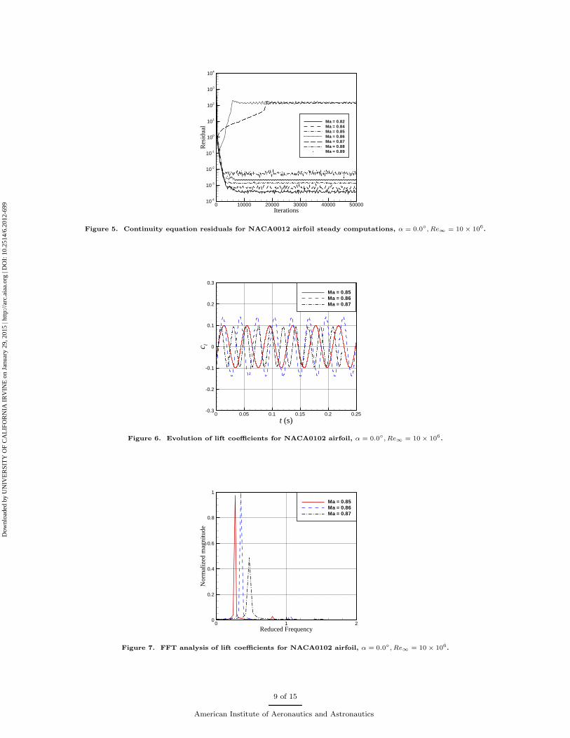
The steady computations had been used to predict the onset of buffet.22 Furthermore, a good convergencewith steady methods probably means good numerical and flow stability. Figure 5 shows continuity equationresiduals history at freestream Mach numbers from 0.82 to 0.89 at zero angle of attack for Reynolds number10 million. At Mach number 0.86 and 0.87 the residuals do not converge. The numerical unsteadiness mightbe caused by the buffet phenomenon. It might indicate the buffet happends in Mach number range of 0.86and 0.87. In the next section the unsteady simulations are performed to study the problem.

III.C. Unsteady Flow Simulations

In this section the unsteady flow field simulations for NACA0012 airfoil at freestream Mach numbers from0.82 to 0.89 at zero angle of attack for Reynolds numbers 10.0 million with transition fixed at 5% chordlength are performed to study unsteady viscous flow behaviors.

The computational results reveal that the flow is steady when the Mach number is between 0.82 and0.84. When the Mach number gets to 0.85, the flow suddenly changes into an unsteady oscillatory mode.The shock waves on the upper and lower surfaces of the airfoil begin to move back and forth in a periodicmotion. The unsteadiness is caused by the shock wave interaction with the boundary layer over the airfoilsurface. It can be categorized to type A shock wave motion. The unsteady flow pattern persists as the Machnumber is further increased until it gets to 0.88 where the flow becomes steady again. The buffet occurs in anarrow band of freestream Mach numbers of 0.85-0.87. It is close to the range of freestream Mach numbersof 0.84-0.86 in which multiple solutions occur for the steady, inviscid flow.1 It might indicate the inviscidinstability is another contributing factor to trigger buffet.

Figure 6 shows the lift coefficients evolution history for the three Mach numbers of 0.85, 0.86, and 0.87.The ∆cl is largest when the Mach number is 0.86. It means the unsteadiness is strongest at that Machnumber. This can be also observed in Fig. 7. The FFT amplitudes are normalized by largest peak betweenthe three Mach numbers. When the Mach number is 0.86, FFT has largest amplitude. The amplitude dropsvery quickly as the Mach number increases to 0.87. The lift coefficient oscillation frequency increases asthe Mach number increases. Figure 8 shows the time-averaged isentropic Mach number distribution on theairfoil surface at Mach numbers from 0.82 to 0.89. The time-averaged shock wave positions are determinedwith the positions where isentropic Mach number is 1.0. It is clear to show the time-averaged shock waveposition moves to trailing edge as the Mach number increases. Figure 9 shows time dependent shock wavepositions against Mach number. In the figure the squares are time-averaged shock wave postion. It clearlyshows the flow is steady when Mach number is lower than 0.85 or higher than 0.87. Figure 10 shows theshock oscillation frequency against the distance between the time-averaged shock wave position and thetrailing edge at different Mach numbers. The shock oscillation frequency depends on the shock wave meanposition. The distance between the time-averaged shock wave position and the trailing edge is an importantlength scale to determine shock wave oscillation frequency. This length scale represents the distance whichdisturbance waves travel through .

Figures 11-12 show the Mach number contours and streamlines at 4 sequential time instants during oneperiod of the shock oscillation at Mach number 0.86. The figures show the shock waves on the upper andlower surface of NACA0012 airfoil move back and forth in a periodic motion. As the upper surface shock

4 of 15

American Institute of Aeronautics and Astronautics

Dow

nloa

ded

by U

NIV

ER

SIT

Y O

F C

AL

IFO

RN

IA I

RV

INE

on

Janu

ary

29, 2

015

| http

://ar

c.ai

aa.o

rg |

DO

I: 1

0.25

14/6

.201

2-69

9

wave moving upstream, it becomes weaker and the separation bubble becomes smaller. At the same time thelower surface shock moves downstream and becomes stronger. Stronger shock induces flow separation. As theseparation region on the lower surface becomes large enough, the lower surface shock wave is pushed upstreamand the upper surface shock wave moves downstream. The consequence of this behavior is an unsteady shockoscillation over the airfoil. Figures 13-15 show pressure oscillation FFT analysis at x/c = 0.7,x/c = 0.9,and x/c = 1.0, respectively. The FFT amplitudes are normalized by the largest peak at x/c = 0.7. Thefigures show there are two disturbance waves which are caused by shock wave interaction with boundarylayer moving to downstream. The phases of movements of waves differ by exactly 180. The two wavesinteract at the trailing edge. It offers the possibility of elimination of buffet by blocking the path of thedisturbance waves interact.

III.D. Reynolds Number effect

In the previous section C the unsteady flow simulations for NACA0012 airfoil are performed at Reynoldsnumber 10 million. In order to study the effect of Reynolds number unsteady flow simulations are run at3.0 million.

Figure 16 shows the lift coefficients evolution history for the three Mach numbers of 0.85, 0.86, and0.87. ∆cl for the three Mach numbers at Reynolds number 3.0 million are smaller compared with 10 millionresults. It means the unsteadiness is weaker at lower Reynolds number. Figure 17 shows FFT analysis of liftcoefficients. The FFT amplitudes are normalized by largest peak between the three Mach numbers. Figure18 shows the time-averaged isentropic Mach number distribution on the airfoil surface at Mach numbers from0.85 to 0.87. It is clear to show the time-averaged shock wave position moves to upstream as the Reynoldsnumber decreased to 3.0 million. Figure 19 shows the shock oscillation frequency against the distance betweenthe time-averaged shock wave position and the trailing edge at different Mach number 0.85, 0.86, and 0.87.Since the time-averaged shock wave positions move to upstream at Reynolds number 3.0 million, the shockoscillation frequencies become smaller. In order to verify the computational results, transonic wind tunnelunsteady pressure measurements are performed for NACA0012 airfoil at Mach numbers from 0.80 to 0.89at zero angle of attack for Reynolds number 3.0 million. The experiment results without correction showthe buffet onset Mach number 0.88. In general, the wind tunnel sidewall interference would decrease theMach number in the core flow. So the experiment predicts higher buffet onset point. Figure 20 shows thecomparison of time-averaged pressure distribution on the NACA0012 surface between computational andexperimental23 data. In the figure the computational Mach number is 0.85 and the experimental Machnumber is 0.88. The time-averaged shock wave positions are very close. Figure 21 shows the comparison ofpressure oscillation FFT analysis at x/c = 0.75. It shows the primary frequencies of pressure oscillation arevery close. Again it shows it is reasonable to use time-averaged shock wave position as shock wave motionlength scale.

III.E. Elimination of Buffet by Trailing Edge Splitter Plate

In the previous section C the unsteady flow field behaviors of buffet are studied. During the shock oscillationperiod the upper and lower surface shock waves move back and forth, and the disturbance information ofupper and lower side surface are exchanged through the trailing edge of the airfoil. If we can somehow blockthe path of the information exchange, the buffet might be alleviated or eliminated. In this study the addingtrailing edge splitter plate method is studied.13 Two different length plates are used which are shown in Fig.22. The corresponding pressure oscillation contours on the upper surface of NACA0012 airfoil are shown inFig. 23. When the short plate with 6.0% of chord length is used the flow is still unsteady. But the flowbecomes steady when the long plate with 25.0% of chord length is used. The adding trailing edge splitterplate method can be successfully used to eliminate buffet.

IV. Conclusion

A computational study is conducted on the flow field of NACA0012 airfoil at freestream Mach numbersfrom 0.82 to 0.89 at zero angle of attack for Reynolds numbers 3.0 and 10.0 million with transition fixedat 5% chord length. Computational results show the buffet occurs in a narrow band of freestream Machnumbers from 0.85 to 0.87. It is very close to the range of freestream Mach numbers in which multiplesolutions occur for the steady, inviscid flow. It shows very interesting relation between buffet in viscous flow

5 of 15

American Institute of Aeronautics and Astronautics

Dow

nloa

ded

by U

NIV

ER

SIT

Y O

F C

AL

IFO

RN

IA I

RV

INE

on

Janu

ary

29, 2

015

| http

://ar

c.ai

aa.o

rg |

DO

I: 1

0.25

14/6

.201

2-69

9

and multiple solution in inviscid flow. The unsteady shock wave motion frequency is significantly correlatedto the time-averaged shock wave position. The effect of Reynolds number on unsteady flow field is studied.The time-averaged shock wave position moves to upstream as Reynolds number decreases. The shock motionfrequency decreases as well. The computational results are further validated using present transonic windtunnel tests. Flow buffet can be eliminated by adding tailing edge splitter plate with sufficient length.

References

1Liu, Y., Liu, F., and Luo, S., “Abstract: MX.00004 : Linear Stability Analysis on Multiple Solutions of Steady TransonicSmall Disturbance Equation,” APS, Nov. 2010.

2Steinhoff, J. and Jameson, A., “Multiple Solutions of Transonic Potential Flow Equation,” AIAA Journal , Vol. 20, No. 11,1982, pp. 1521–1525.

3Luo, S., Shen, H., and Liu, P., “Transonic Small Transverse Perturbation Equation and its Computation,” Proc. Sym-posium on Computing the Future II: Computational Fluid Dynamics Advances and Applications, ed. D. A. Caughey and M.M. Hafez, 1998.

4Salas, M. D., Jameson, A., and Melnik, R. E., “A Comparative Study of the Nonuniqueness problem of the PotentialEquation,” AIAA 1983-1888, July 1983.

5Williams, M. H., Bland, S. R., and Edwards, J. W., “Flow Instablities in Transonic Small-Disturbance Theory,” AIAA

Journal , Vol. 23, No. 10, 1985, pp. 1491–1496.6Jameson, A., “Airfoils admitting non-unique solutions of Euler Equations,” AIAA 1991-1625, June 1991.7Ivanova, A. V. and Kuz’min, A. G., “Nonuniqueness of the Transonic Flow past an Airfoil,” Fluid Dynamics, Vol. 39,

No. 4, 2004, pp. 642–448.8Hafez, M. M. and Guo, W. H., “Nonuniqueness of Transonic Flows,” Acta Mechanica, Vol. 138, 1999, pp. 177–184.9Hafez, M. M., “Non-uniqueness Problems in Transonic Flows,” Computational Fluid Dynamics, Vol. 11, No. 1, 2002,

pp. 371–376.10Caughey, D. A., “Stability of Unsteady Flow past Airfoils Exhibiting Transonic Non-uniqueness,” Computational Fluid

Dynamics, Vol. 13, No. 3, 2004, pp. 427–438.11Crouch, J. D., Garbaruk, A., Magidov, D., and Travin, A., “Origin of Transonic Buffet on Aerofoil,” J. Fluid Mech.,

Vol. 628, 2009, pp. 357–369.12Mcdevitt, J. B. and Okuno, A. F., “Static and Dynamic Pressure Measurements on a NACA 0012 Airfoil in the Ames

High Reynolds Number Facility,” NASA TP 2485, 1985.13Mcdevitt, J. B., “Supercitical Flow About a Thick Circular-Arc Airofil,” NASA TM 78549, 1979.14Mcdevitt, J. B., Levy, J. J., and Deiwert, G. S., “Transonic flow about a thick circular-arc airfoil,” AIAA Journal ,

Vol. 14, No. 5, 1976, pp. 606–613.15Levy, J. J., “Experimental and computational steady and unsteady transonic flows about a thick airfoil,” AIAA Journal ,

Vol. 16, No. 6, 1978, pp. 564–572.16Marvin, J. G. and Levy, J. J., “Turbulence modelling for unsteady transonic flows,” AIAA Journal , Vol. 18, No. 5, 1980,

pp. 489–496.17Xiong, J., Nielsen, P., Liu, F., and Papamoschou, D., “Computation of High-Speed Coaxial Jets with Fan Flow Deflec-

tion,” AIAA Journal , Vol. 48, No. 10, 2010, pp. 2249–2262.18Jameson, A., Schmift, W., and Turkel, E., “Numerical Solutions of the Euler Equations by Finite Volume Methods Using

Runge-Kutta Time Stepping Schemes,” AIAA 1981-1259, Janurary 1981.19Menter, F., “Two-Equation Eddy-Viscosity Turbulence Models for Engineering Applications,” AIAA Journal , Vol. 32,

No. 8, 1994, pp. 1598–1605.20Liu, F. and Zheng, X., “A Strongly Coupled Time-Marching Method for Solving the Navier-Stokes and k-ω Turbulence

Model Equations with Multigrid,” Journal of Computational Physics, Vol. 128, No. 10, 1996, pp. 257–284.21Xiao, Q., Tsai, H. M., and Liu, F., “Numerical Study of Transonic Buffet on a Supercritical Airfoil,” AIAA Journal ,

Vol. 44, No. 3, 2006, pp. 620–628.22Chung, I., Lee, D., and Reu, T., “Prediction of Transonic Buffet Onset for An Airfoil with Shock Induced Separation

Bubble Using Steady Navier-Stokes Solver,” AIAA 2002-2934, June 2002.23Zhao, Z., Gao, C., Ren, X., Xiong, J., , Liu, F., and Luo, S., “Pressure Distributions over NACA 0012 Airfoil in a

Transonic Wind Tunnel,” Submitted to 42th AIAA Fluid Dynamics Conference.

6 of 15

American Institute of Aeronautics and Astronautics

Dow

nloa

ded

by U

NIV

ER

SIT

Y O

F C

AL

IFO

RN

IA I

RV

INE

on

Janu

ary

29, 2

015

| http

://ar

c.ai

aa.o

rg |

DO

I: 1

0.25

14/6

.201

2-69

9

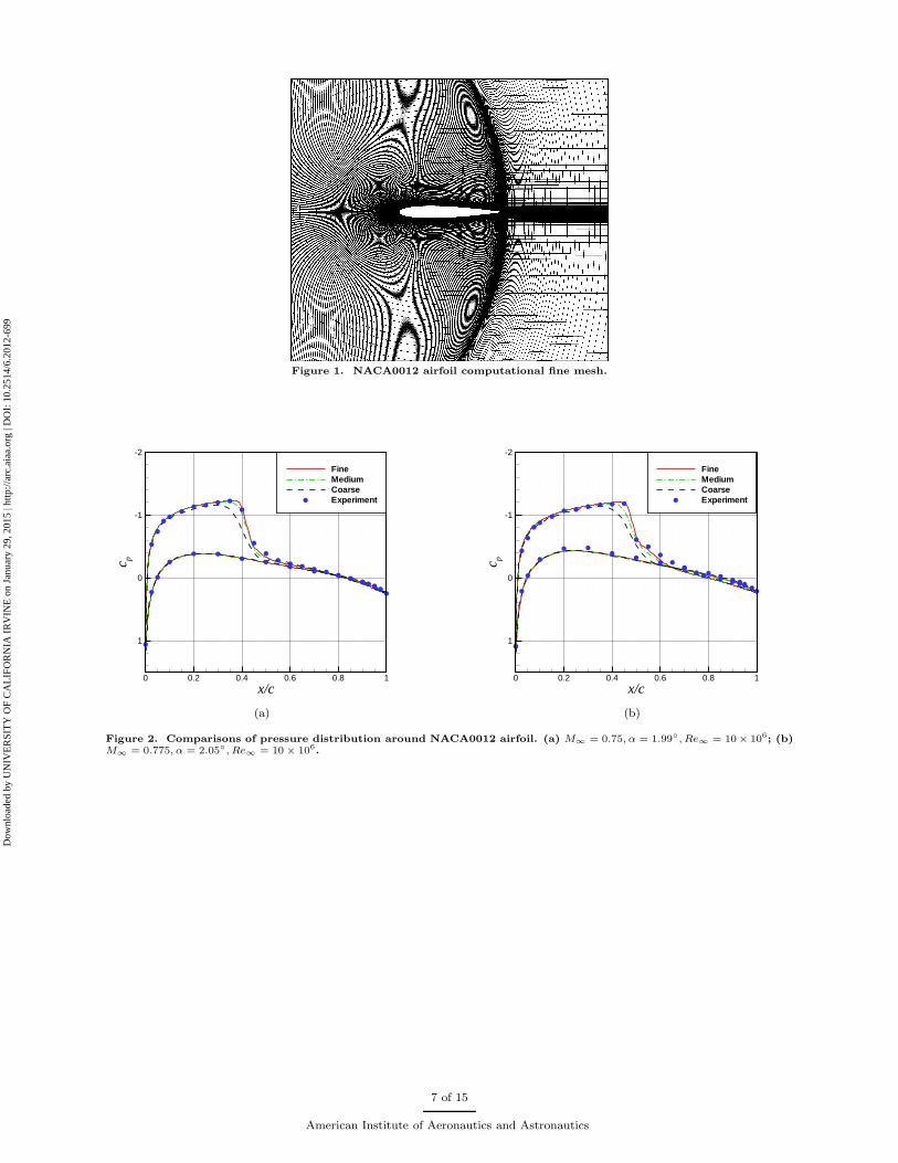
Figure 1. NACA0012 airfoil computational fine mesh.

x/c

c p

0 0.2 0.4 0.6 0.8 1

-2

-1

0

1

FineMediumCoarseExperiment

(a)

x/c

c p

0 0.2 0.4 0.6 0.8 1

-2

-1

0

1

FineMediumCoarseExperiment

(b)

Figure 2. Comparisons of pressure distribution around NACA0012 airfoil. (a) M∞ = 0.75, α = 1.99, Re∞ = 10 × 106; (b)M∞ = 0.775, α = 2.05, Re∞ = 10 × 106.

7 of 15

American Institute of Aeronautics and Astronautics

Dow

nloa

ded

by U

NIV

ER

SIT

Y O

F C

AL

IFO

RN

IA I

RV

INE

on

Janu

ary

29, 2

015

| http

://ar

c.ai

aa.o

rg |

DO

I: 1

0.25

14/6

.201

2-69

9

t (s)

c l

0 0.05 0.1 0.15 0.2 0.25

-0.5

-0.25

0

0.25

0.5

(a)

Reduced frequency

Nor

mal

ized

mag

nitu

de

0 0.5 1 1.5 20

0.2

0.4

0.6

0.8

1

(b)

Figure 3. Evolution of lift coefficient and FFT analysis for 18% thick arcfoil, M∞ = 0.76, α = 0.0, Re∞ = 11 × 106. (a)Lift coefficient; (b) FFT analysis.

x/c

c p

0 0.2 0.4 0.6 0.8 1

-2

-1

0

1

ExperimentComputation

Figure 4. Comparison of time-averaged pressure distribution around 18% thick arcfoil, M∞ = 0.76, α = 0.0, Re∞ =11 × 106.

8 of 15

American Institute of Aeronautics and Astronautics

Dow

nloa

ded

by U

NIV

ER

SIT

Y O

F C

AL

IFO

RN

IA I

RV

INE

on

Janu

ary

29, 2

015

| http

://ar

c.ai

aa.o

rg |

DO

I: 1

0.25

14/6

.201

2-69

9

IterationsR

esid

ual

0 10000 20000 30000 40000 5000010-4

10-3

10-2

10-1

100

101

102

103

104

Ma = 0.82Ma = 0.84Ma = 0.85Ma = 0.86Ma = 0.87Ma = 0.88Ma = 0.89

Figure 5. Continuity equation residuals for NACA0012 airfoil steady computations, α = 0.0, Re∞ = 10 × 106.

t (s)

c l

0 0.05 0.1 0.15 0.2 0.25-0.3

-0.2

-0.1

0

0.1

0.2

0.3

Ma = 0.85Ma = 0.86Ma = 0.87

Figure 6. Evolution of lift coefficients for NACA0102 airfoil, α = 0.0, Re∞ = 10 × 106.

Reduced Frequency

Nor

mal

ized

mag

nitu

de

0 1 20

0.2

0.4

0.6

0.8

1

Ma = 0.85Ma = 0.86Ma = 0.87

Figure 7. FFT analysis of lift coefficients for NACA0102 airfoil, α = 0.0, Re∞ = 10 × 106.

9 of 15

American Institute of Aeronautics and Astronautics

Dow

nloa

ded

by U

NIV

ER

SIT

Y O

F C

AL

IFO

RN

IA I

RV

INE

on

Janu

ary

29, 2

015

| http

://ar

c.ai

aa.o

rg |

DO

I: 1

0.25

14/6

.201

2-69

9

Figure 8. Time-averaged isentropic Mach number distributions around NACA0012 airfoil, α = 0.0, Re∞ = 10 × 106.

Figure 9. Shock wave position against freestream Mach number for NACA0012 airfoil, α = 0.0, Re∞ = 10 × 106. (Bluesquare denotes time-averaged shock wave position)

1/(1-xsm/c)

Red

uced

Fre

quen

cy

3.5 4 4.5 5 5.5 60

0.25

0.5

0.75

1

Figure 10. Shock wave oscillation frequency position against the distance between time-averaged shock wave positionand trailing edge for NACA0012 airfoil, M∞ = 0.85 − 0.87, α = 0.0, Re∞ = 10 × 106.

10 of 15

American Institute of Aeronautics and Astronautics

Dow

nloa

ded

by U

NIV

ER

SIT

Y O

F C

AL

IFO

RN

IA I

RV

INE

on

Janu

ary

29, 2

015

| http

://ar

c.ai

aa.o

rg |

DO

I: 1

0.25

14/6

.201

2-69

9

(a) (b)

(c) (d)

Figure 11. Mach number contours at different instant time in one period around the NACA0012 airfoil, M∞ = 0.86, α =0.0, Re∞ = 10 × 106. (a)T = t1; (b)T = t2; (c)T = t3; (d)T = t4;

(a) (b)

(c) (d)

Figure 12. Streamlines at different instant time in one period around the NACA0012 airfoil, M∞ = 0.86, α = 0.0, Re∞ =10 × 106. (a)T = t1; (b)T = t2; (c)T = t3; (d)T = t4;

11 of 15

American Institute of Aeronautics and Astronautics

Dow

nloa

ded

by U

NIV

ER

SIT

Y O

F C

AL

IFO

RN

IA I

RV

INE

on

Janu

ary

29, 2

015

| http

://ar

c.ai

aa.o

rg |

DO

I: 1

0.25

14/6

.201

2-69

9

Pressure fluctuation reduced frequence

Nor

mal

ized

mag

nitu

de

0 0.5 1 1.5 20

0.2

0.4

0.6

0.8

1

x/c=0.7, upperx/c=0.7, lower

(a)

Pressure fluctuation reduced frequency

Pha

se(R

ad)

0 0.5 1 1.5 2

-3

-1.5

0

1.5

3

4.5 x/c=0.7, upperx/c=0.7,lower

(b)

Figure 13. FFT analysis of pressure oscillation at x/c = 0.7 for NACA0012 airfoil, M∞ = 0.86, α = 0.0, Re∞ = 10 × 106.(a) FFT amplitude; (b) FFT phase.

Pressure fluctuation reduced frequence

Nor

mal

ized

mag

nitu

de

0 0.5 1 1.5 20

0.2

0.4

0.6

0.8

1

x/c=0.9, upperx/c=0.9, lower

(a)

Pressure fluctuation reduced frequency

Pha

se(R

ad)

0 0.5 1 1.5 2

-3

-1.5

0

1.5

3

4.5 x/c=0.9, upperx/c=0.9,lower

(b)

Figure 14. FFT analysis of pressure oscillation at x/c = 0.9 for NACA0012 airfoil, M∞ = 0.86, α = 0.0, Re∞ = 10 × 106.(a) FFT amplitude; (b) FFT phase.

Pressure fluctuation reduced frequence

Nor

mal

ized

mag

nitu

de

0 0.5 1 1.5 20

0.2

0.4

0.6

0.8

1

x/c=1.0

(a)

Pressure fluctuation reduced frequency

Pha

se(R

ad)

0 0.5 1 1.5 2

-3

-1.5

0

1.5

3

4.5 x/c=1.0

(b)

Figure 15. FFT analysis of pressure oscillation at x/c = 1.0 for NACA0012 airfoil, M∞ = 0.86, α = 0.0, Re∞ = 10 × 106.(a) FFT amplitude; (b) FFT phase.

12 of 15

American Institute of Aeronautics and Astronautics

Dow

nloa

ded

by U

NIV

ER

SIT

Y O

F C

AL

IFO

RN

IA I

RV

INE

on

Janu

ary

29, 2

015

| http

://ar

c.ai

aa.o

rg |

DO

I: 1

0.25

14/6

.201

2-69

9

t (s)c l

0 0.05 0.1 0.15 0.2 0.25-0.3

-0.2

-0.1

0

0.1

0.2

0.3

Ma = 0.85Ma = 0.86Ma = 0.87

Figure 16. Evolution of lift coefficients for NACA0102 airfoil, α = 0.0, Re∞ = 3.0 × 106.

Reduced Frequency

Nor

mal

ized

mag

nitu

de

0 1 20

0.2

0.4

0.6

0.8

1

Ma = 0.85Ma = 0.86Ma = 0.87

Figure 17. FFT analysis of lift coefficients for NACA0102 airfoil, α = 0.0, Re∞ = 3.0 × 106.

x/c

Mis

0 0.2 0.4 0.6 0.8 10

0.2

0.4

0.6

0.8

1

1.2

1.4

Ma=0.85, Re=3.0x106

Ma=0.85, Re=10.0x106

Ma=0.86, Re=3.0x106

Ma=0.86, Re=10.0x106

Ma=0.87, Re=3.0x106

Ma=0.87, Re=10.0x106

Figure 18. Time-averaged isentropic Mach number distributions around NACA0012 airfoil, α = 0.0.

13 of 15

American Institute of Aeronautics and Astronautics

Dow

nloa

ded

by U

NIV

ER

SIT

Y O

F C

AL

IFO

RN

IA I

RV

INE

on

Janu

ary

29, 2

015

| http

://ar

c.ai

aa.o

rg |

DO

I: 1

0.25

14/6

.201

2-69

9

1/(1-xsm/c)R

educ

edF

requ

ency

3 4 5 60

0.2

0.4

0.6

Re=3.0x106

Re=10.0x106

Figure 19. Shock wave oscillation frequency position against the distance between time-averaged shock wave positionand trailing edge for NACA0012 airfoil, M∞ = 0.85 − 0.87, α = 0.0.

x/c

c p

0 0.2 0.4 0.6 0.8 1

-2

-1

0

1

Experiment (lower_surface)Experiment (upper_surface)Computation

Figure 20. Comparison of time-averaged pressure distribution around NACA0012 airfoil, α = 0.0, Re∞ = 3.0 × 106.

Pressure oscillation frequency (Hz)

Nor

mal

ized

mag

nitu

de

100 200 300 400 5000

0.2

0.4

0.6

0.8

1

ExperimentComputation

Figure 21. FFT analysis of pressure oscillation at x/c = 0.75 for NACA0012 airfoil, α = 0.0, Re∞ = 3.0 × 106

14 of 15

American Institute of Aeronautics and Astronautics

Dow

nloa

ded

by U

NIV

ER

SIT

Y O

F C

AL

IFO

RN

IA I

RV

INE

on

Janu

ary

29, 2

015

| http

://ar

c.ai

aa.o

rg |

DO

I: 1

0.25

14/6

.201

2-69

9

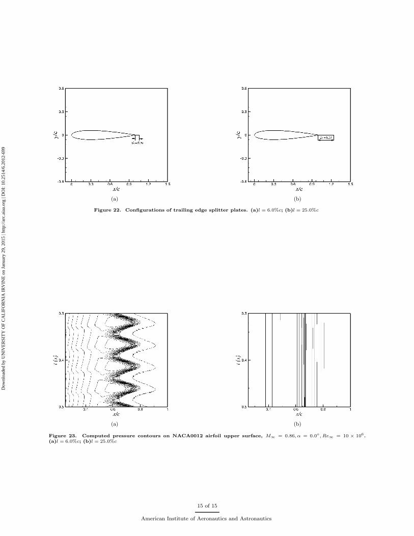
(a) (b)

Figure 22. Configurations of trailing edge splitter plates. (a)l = 6.0%c; (b)l = 25.0%c

(a) (b)

Figure 23. Computed pressure contours on NACA0012 airfoil upper surface, M∞ = 0.86, α = 0.0, Re∞ = 10 × 106.(a)l = 6.0%c; (b)l = 25.0%c

15 of 15

American Institute of Aeronautics and Astronautics

Dow

nloa

ded

by U

NIV

ER

SIT

Y O

F C

AL

IFO

RN

IA I

RV

INE

on

Janu

ary

29, 2

015

| http

://ar

c.ai

aa.o

rg |

DO

I: 1

0.25

14/6

.201

2-69

9