computational analysis of a drag reducing cone grid

Computational Analysis ofa Drag reducing Cone Grid

A finite volume simulation of the gecko'saerodynamic skin

Anders Utnes

Master thesis at The Mathematical Institute

UNIVERSITY OF OSLO

21.12.2017

© Anders Utnes

2017

Computational Analysis of a Dragreducing Cone Grid

Anders Utnes

http://www.duo.uio.no/

Print: Reprosentralen, University of Oslo

http://www.duo.uio.no/

As I finish my education, I find there are no shortage of people to thank. So in order of abstract

proximity, I wish to thank...

... my supervisor, Mikael Mortensen, for guidance and patience both during this thesis and in many

of the related subjects I have studied.

... my co-supervisor, Murat Tutkun, for the experimental work that this thesis is based upon, and for

lending me his experience and insigth.

... the rest of the professors at the university, for responding to stupidity with wisdom.

... my friends, for keeping me sane during this endevour.

... my blue collar colleges at Hydro and UNU, for reminding me to always keep in mind the

practicality of my approach.

...my family. For their always loyal support.

...and a group of hungry nomads somewhere in the middle east around 8000 years ago, for inventing

agriculture and thus getting the ball rolling. While they probably didn't have my thesis in mind at

the time, I feel confident that I could not have done it without them and that they don't get enough

recognition for their work.

AbstractA recent study at the University of Illinois [1], inspired by the skin of geckos, explored the benefits

of introducing a grid of cones to a airfoil and if this could possibly have effects that reduce the drag

forces over a surface. The implications of this are enormous, as energy loss due to drag forces are a

major issue for all movement on earth, becoming more and more problematic as the velocity

increase. Any method to conclusively reduce this drag, even if only by a small amount, would be

able to save untold amounts of fuel with all the environmental and economic benefits that would

entail.

This thesis aims to explore is whether or not the introduction of a grid of cones like the one used in

the aforementioned study can create an beneficial drag reducing phenomena for a surface. To

accomplish this we perform a comparison of a surface with and without a cone grid using

Computational Fluid Dynamics techniques. The problem is constrained into a simplified situation

more suited for study, in this case a recycled channel flow, and the volume within is then discretized

into a mesh of finite cells. Then the Navier-Stokes equations are solved for the entire domain, using

Large Eddy Simulation and the Spalart-Allmaras turbulence model.

The results are negative, as we see that the cone grid suffers a higher drag coefficient than a

corresponding flat plate, both for a slow laminar flow and for a high velocity turbulent flow. While

there is a negligible difference between the two in the laminar case, the turbulent case see an

increase in the average drag coefficient by 286% by adding the cones. The vortexes formed are

discussed in detail, and possible error sources are discussed in detail.

A script for easily generating a cone grid mesh has also been developed and is added to the

attachments, to make it easier for any later reproduction studies, if applicable.

Table of ContentsAbstract.................................................................................................................................................4Table of Contents..................................................................................................................................5Introduction..........................................................................................................................................6Method..................................................................................................................................................7

Basic problem definition..................................................................................................................7Description of the numerical method...............................................................................................8

The numerical differential schemes used in the simulations:.....................................................9Detailed description of the cones used............................................................................................9Description of the boundary conditions used................................................................................10

Initial condition for the internal volume:..................................................................................10Inlet and outlet boundaries........................................................................................................11Side boundaries.........................................................................................................................11Walls..........................................................................................................................................12

Description of the mesh.................................................................................................................12Calculation of Drag Coefficient.....................................................................................................15Evaluation and eventual rejection of other approaches.................................................................16

Results................................................................................................................................................17Laminar model...............................................................................................................................17Turbulent Case...............................................................................................................................19

Discussion...........................................................................................................................................25Inherent errors from numerical solutions.......................................................................................25Possible errors from basic problem constraints.............................................................................25The existence of turbulence in the high Reynolds number case....................................................26Mesh size, and possible impact......................................................................................................27Wallfunction for νt , Spalding........................................................................................................28Turbulence semi-steady-state assumption.....................................................................................28Numerical Artifacts........................................................................................................................28

Conclusion..........................................................................................................................................30List of references................................................................................................................................32Attachments........................................................................................................................................33

Script for generating the 6x12 cone grid mesh..............................................................................33

IntroductionThis is a one-semester thesis, finishing a Masters Degree in Applied Mathematics and Fluid

dynamics at the University of Oslo autumn 2017.

Researchers with the University of Illinois [1] has recently done a experimental study linking

a grid system of cones covering an airfoil to a total decrease in drag force over the airfoil as a

result of a change in flow separation. This was inspired by biological textures found on the

surface on the skin of geckos, a field of study that may have untapped potential.

One of the many implications of that study are that a flat plate covered with this texture may

have a lower total aerodynamic drag than a perfectly plain flat plate. If this is true, it could

potentially have enormous ramifications for all objects in the world moving fast enough that

drag force becomes a non-negligible issue.

To explore this I have constrained the problem into a testable and quantifiable experiment that

I analyze using Computational Fluid Dynamic techniques. I first define a open channel

covered with walls only on the top and bottom, then let the inlet, outlet and sides be infinitely

recycled until we approach a steady or semi-steady state. To avoid the loss of energy, I add a

source term to the momentum equation designed to keep the mean velocity of the entire

volume constant.

I then run 4 separate experiments where I first solve the case for a low velocity laminar flow

in a plain channel; then the same flow velocity but with the bottom of the channel covered

with the cone grid; then a high velocity, turbulent flow in a empty channel; and a high

velocity flow with a cone covered channel. These 4 cases are then directly compared, to get a

understanding of the benefits from covering or not covering the bottom plate with the texture.

I then discuss how the results can be evaluated, what potential weaknesses may be inherent in

my approach, and how to mitigate them. Finally I summarize the results in a conclusion, and

looks at how they compare with my expectations.

As a attachment I have provided a script I designed to generate the mesh I ended up using.

6

MethodBasic problem definition

We are here focusing on one essential question:

Is it possible that by adding a cone grid to a flat plate we could decrease the total amount of

drag force on the plate as a fluid flows over it?

To answer this it is essential to run two kinds of simulations: One with a perfectly flat plane,

and one with a coned surface. These two cases can then be compared directly. In a perfect

world we would research this for a infinite plane, with a infinite fluid flowing over it. Further

more, we would like to achieve perfect knowledge of the drag development for all fluids and

for all velocities. This is obviously problematic, as my resources are generally not described

as “infinite” by anyone with a basic understanding of both mathematics and my wallet.

So in order to better solve this problem we constrict our approach to a few useful

approximations. First of all, we only investigate the flow for a single fluid with a constant

viscosity, similar to the one in the experimental study.

Secondly, we only investigate two velocities: A laminar flow with a Reynolds number of 103;

and a high velocity turbulent flow with a Reynolds number of 105. This gives us 4 discrete

cases that can be directly compared with each other. The Reynolds number is a dimensionless

number that gives a comparison between the inertia and viscous forces in a system, and a high

number (above ~3000) is traditionally an indicator of possible turbulence.

Third, we only investigate a finite section of the infinite plate, and only a finite volume above

it. To keep our simulation accurate, we impose a recycling condition on the boundary of this

finite space as we move over the plate, effectively letting us follow the flow of fluid further

and further downstream as it develops into what we hope to be a semi-steady state. To keep

the flow controlled, we introduce a upper wall and effectively create a open channel flow.

Introducing a coned grid will place 85 μm high obstacles on the bottom, which we expect to

constrict the inlet. My co-supervisor Tutkun advised me to keep this constriction below 3%,

prompting us to set the total height of the channel to 3000 μm.

Fourth, we discretize the volume into a mesh of finite volume cells, and apply Computational

Fluid Dynamic techniques to numerically solve the Navier-Stokes equations for the mesh.

7

The end result is a solution that is achievable, testable, and evaluable.

Description of the numerical method

Computational Fluid Dynamics involves numerically approximating the Navier-Stokes

equations on a discretized domain. In this case, we are using the finite volume method, built

into the open-source program OpenFoam.

The full Navier-Stokes equations are incredibly computationally expensive to solve due to the

incredible amount of small turbulent vortexes, so we make use of a system called Large Eddy

Simulation. With this system only the large vortexes are fully computed, and the effects of the

smaller vortexes are simply modeled. The equations are further simplified by assuming that

the fluid will behave as incompressible. Equation 1 shows us the LES momentum equations,

with reference to the thesis by E. Villiers [2], where ū is the filtered velocity field vector; p is

the filtered pressure field; ν is the viscosity; ρ is the density; and τ is the sub grid-scale stress

tensor.

1)∂ u∂ t

+∇·(u u)=−∇ p

ρ +∇·ν(∇u+∇uT)+∇· τ , ∇· u=0

To calculate the turbulence I make use of the Spalart-Allmaras DDES model, a model

originally designed to be used for high turbulence aerodynamics. Since this model has grown

steadily in popularity it became my first choice. I also made some attempts at using a

Smagorinsky–Lilly model, but I found the Spalart-Allmaras model converged much more

reliably. Equation set 2 shows how the eddy viscosity (νt) is connected to a Spalart-Allmaras

variable (ῦ). The constants are: cb1= 0.1355, cσ= 2/3, cb2= 0.622, κ= 0.41, cw1=cb1/κ2+ (1+

cb2)/cσ, cw2= 0.3, cw3= 2, cv1= 7.1 ; and ω is the vorticity magnitude.

2) D νDt

=cb1 S ν+1cσ

[∇·((ν+ ν)∇ν)+cb2(∇ν)2]− cw1 f w(

νyw

)2

, τ=ν t(∇u+∇uT) ,

ν t=ν f v 1 , f v1=X 3

X 3+cv1

3, X ≡

νν

, S ≡ ω+ν

κ2 y w2

f v2 , f v2=1−X

1+X f v1

,

f w=g (1+cw3

6

g 6+cw3

6 )16 , g=r+cw2(r6− r ) , r=

ν

S κ2 yw2

.

8

The numerical differential schemes used in the simulations:

Reference for the schemes are the OpenFoam User Guide [3] and an analysis by Hrvoje Jasak

[4].

Time differential terms: Backwards difference. This is a second order implicit scheme.

Gradient terms: Cell limited Gauss Linear 1 for velocity and turbulent viscosity, and Gauss

Linear for everything else. Cell limited <SCHEME> 1 means that some accuracy is sacrificed

for stability. Gauss <SCHEME> means that the scheme makes use of Gaussian integration

and linear means that a central difference interpolation is used.

Divergence terms: Gauss LUST unlimitedGrad(U) for velocity and Gauss limitedLinear 1 for

the Spalart-Allmaras variable. LUST refers to a mixed 75% linear scheme and 25% linear

upwind scheme. limitedLinear 1 refers to the TVD scheme and the Sweby limiter function.

Gradients normal to the Surface: limited corrected 0.33. Since this is a unstructured mesh,

orthogonality is a issue and we use a non-orthogonal correction term. This term is then

modified with a relaxation factor of 33%.

Laplacian terms: Gauss linear limited corrected 0.33. This takes the form of Gauss

<interpolation scheme> <surface gradient scheme>, both of which are mentioned above.

Point to point Interpolation: Linear. This refers to what is commonly known as central

difference.

The equation set is then solved using the PISO algorithm.

Detailed description of the cones used

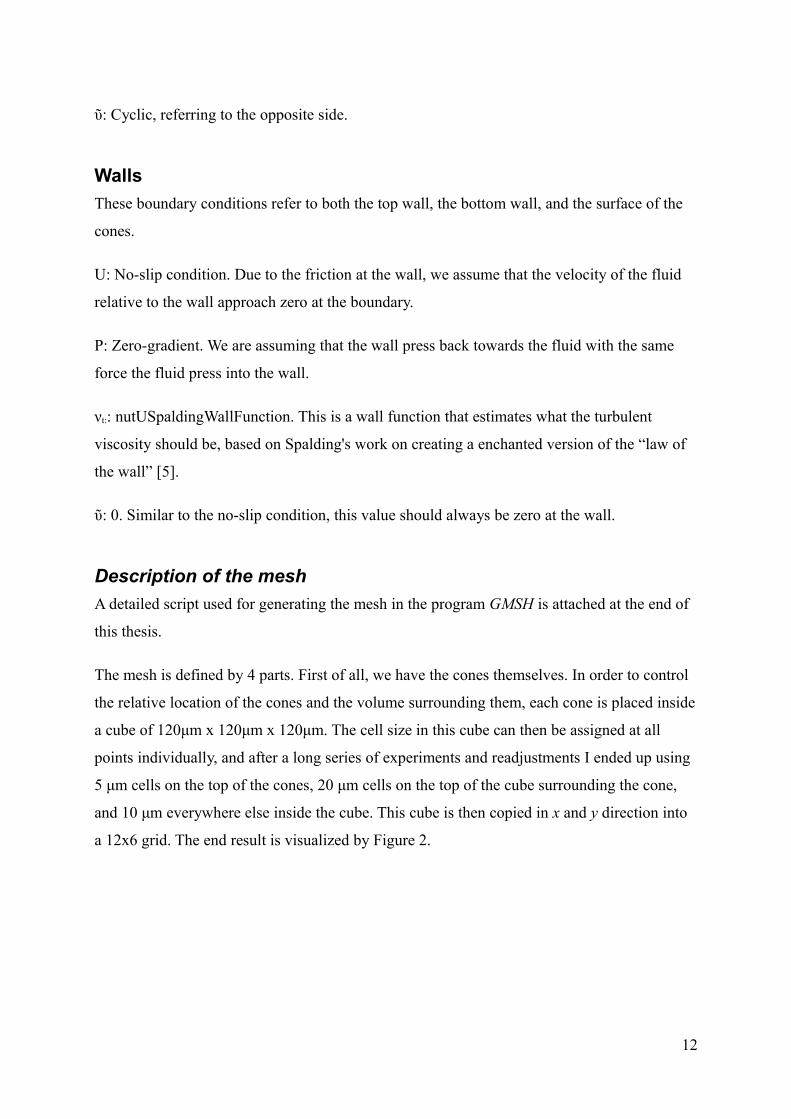
The cones are placed in a 3D Cartesian system with exactly 120 μm between each cone in

both x and y directions. The cones have a diameter of 40 μm at the bottom, are 85 μm tall, and

starts expanding at z=65 μm to a diameter of 85 μm at the top. This is visualized by Figure 1.

9

Description of the boundary conditions used

The numerical model we have chosen to use require us to define boundary conditions for 4

variables at all boundaries and for the internal condition: Velocity vector (U), pressure (P),

Turbulent viscosity (νt), and the Spalart-Allmaras variable (ῦ).

Note that the viscosity of the fluid (ν) is chosen as 0.0000011 m2/s, in accordance with the

experimental study this thesis is based on.

Initial condition for the internal volume:

U: 0.367 m/s in the x direction for the laminar case, and 36.7 m/s for the turbulent case. This

is chosen in order to get a Reynolds number of 103 and 105 respectively, with a characteristic

height of the channel as 0.003 m and a viscosity of 0.0000011 m2/s.

P: 0 at all points. As the absolute pressure is irrelevant to a incompressible fluid, only the

relative value as the simulation progress is relevant.

νt:: 0.00002 m2/s on each point. Irrelevant for the laminar solution, and for the turbulent

solution it is chosen as twice the size of the fluid viscosity, to ensure that the simulation would

10

Figure 1: Sketch of a cone. All dimensions are in μm.

“start up” fully turbulent.

ῦ: 0.00002 m2/s on each point, using the same argument as νt.

In addition, the fvOptions function in OpenFoam is used to apply a source term to the

momentum equation of the type meanVelocityForce. This is a function specifically designed

to keep the average velocity constant, and is required to avoid the system from losing energy

over time. The values here mimic the start condition, being 0.367 m/s in the x direction for the

laminar case and 36.7 m/s for the turbulent case.

Inlet and outlet boundaries

I will refer to the boundary at x=0 as inlet, even through a cyclic simulation technically does

not have a inlet. The boundary at x=1440 μm is likewise refereed to as an outlet.

U: Cyclic, referring to the opposite side. The cyclic condition (often called “periodic”) refers

each cell to a similar cell at the opposite boundary, and matches the values as if they where

placed adjacent to each other. This allows us to reuse the same domain infinitely, as whatever

flow pattern leaves at the outlet returns at the inlet.

P: Cyclic, referring to the opposite side.

νt:: Cyclic, referring to the opposite side.

ῦ: Cyclic, referring to the opposite side.

Side boundaries

The sides at y=0 and y= 720 μm are refereed to the left and right sides, and like the inlet and

outlet they are both cyclic and referring to each other.

U: Cyclic, referring to the opposite side. The cyclic condition refers each cell to a similar cell

at the opposite boundary, and matches the values as if they where placed adjacent to each

other. This allows us to reuse the same domain infinitely, as the inlet flow corresponds to

whatever form the outlet currently have.

P: Cyclic, referring to the opposite side.

νt:: Cyclic, referring to the opposite side.

11

ῦ: Cyclic, referring to the opposite side.

Walls

These boundary conditions refer to both the top wall, the bottom wall, and the surface of the

cones.

U: No-slip condition. Due to the friction at the wall, we assume that the velocity of the fluid

relative to the wall approach zero at the boundary.

P: Zero-gradient. We are assuming that the wall press back towards the fluid with the same

force the fluid press into the wall.

νt:: nutUSpaldingWallFunction. This is a wall function that estimates what the turbulent

viscosity should be, based on Spalding's work on creating a enchanted version of the “law of

the wall” [5].

ῦ: 0. Similar to the no-slip condition, this value should always be zero at the wall.

Description of the mesh

A detailed script used for generating the mesh in the program GMSH is attached at the end of

this thesis.

The mesh is defined by 4 parts. First of all, we have the cones themselves. In order to control

the relative location of the cones and the volume surrounding them, each cone is placed inside

a cube of 120μm x 120μm x 120μm. The cell size in this cube can then be assigned at all

points individually, and after a long series of experiments and readjustments I ended up using

5 μm cells on the top of the cones, 20 μm cells on the top of the cube surrounding the cone,

and 10 μm everywhere else inside the cube. This cube is then copied in x and y direction into

a 12x6 grid. The end result is visualized by Figure 2.

12

To fill the rest of the channel, it is now a matter of attaching a large empty volume on top of

the grid surface. But because we want to control the cell size in different parts of the channel,

we divide this into 3 parts. The second part is a 700 μm high cuboid placed on the top of the

grid. The mesh size is here 20 μm at the bottom and 40 μm a the top. This represent a

boundary layer where the velocity increase as we move farther away from the wall. The final

decision of using a 700 μm distance was made based on a series of early iterations of the

simulation. Figure 3 visualizes the setup.

13

Figure 2: A visualization of the grid density surrounding the cones. The slicing is done using a "crinkle clip" function in the program ParaVeiw, meaning that the cut follows the cell faces and thus gives a great representation of the actual mesh density.

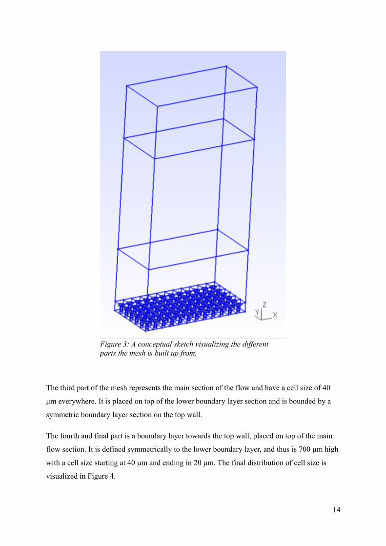
The third part of the mesh represents the main section of the flow and have a cell size of 40

μm everywhere. It is placed on top of the lower boundary layer section and is bounded by a

symmetric boundary layer section on the top wall.

The fourth and final part is a boundary layer towards the top wall, placed on top of the main

flow section. It is defined symmetrically to the lower boundary layer, and thus is 700 μm high

with a cell size starting at 40 μm and ending in 20 μm. The final distribution of cell size is

visualized in Figure 4.

14

Figure 3: A conceptual sketch visualizing the different parts the mesh is built up from.

Calculation of Drag Coefficient

We can imagine the drag force as the wall's resistance to the movement of the fluid. The drag

force also generates vortexes, and results in a large loss of energy over time. It is a huge issue

in fluidmechanics, as reducing it could save unimaginative amounts of energy on a global

scale.

For our purposes we shall investigate this by evaluating the Drag Coefficient, defined in

Equation 3 as the drag force (FD) relative to the area the drag is applied to (A), the density (ρ),

and the velocity of the fluid (U). It is important at this point to note that when the cone grid is

applied to the flat surface, the area of contact increase with the size of the cones. I want to

make clear that I will be using the same reference area for calculation of the drag coefficient

for both the flat plate and the cone grid, in order to compare the two correctly, even as the

cones technically has a much larger area of contact with the fluid.

3) C D=2 F D

U 2 Aρ

Openfoam has a built in function called forceCoeffs that handles the detailed calculation for a

selected boundary, that I made use of to generate the results in the next chapter.

Lastly, I have been overly cautious regarding the appearance of numerical artifacts at the

15

Figure 4: A visualization of the cell density in the mesh. The slicing is done using a "crinkle clip" function in the program ParaVeiw, meaning that the cut follows the cell faces.

boundaries. While I in retrospect believe these effects where less of a issue now than I did in

the start of the project, I have consistently been avoiding using the outmost layer of cones for

the calculation of the drag coefficient. While this does in no way introduce any errors, I doubt

this actually removed any either, and it may have made the final result slightly more sensitive

to stochastic fluctuations since the reference area is smaller.

Evaluation and eventual rejection of other approaches

The generation of the mesh and proper density of it was a large issue especially in the start of

the project. My original approach was to use a program called FreeCAD to generate stl files

of the boundaries, then use the program snappyHexMesh built into OpenFoam to generate a

mesh. While this approach had a lot of benefits it had a major weakness: It would generate

approximations on the corners of the mesh, giving rounded corners with non-plane cyclic

boundaries. This generated inherent errors that made the approach non-feasible.

For the mesh itself I originally made attempts at generating a long channel with a traditional

inlet and outlet, but this approach proved unfeasible for a number of reasons, most

prominently the enormous computational cost it would require.

Attempts was also made at making a high density mesh of only a few cones and a lower

channel roof, solved using the Smagorinsky–Lilly turbulence model, and compare this with

the other results. It was unfortunately prone to severe convergation problems, and I ultimately

ended up not having the resources (time) to spare.

16

ResultsThe results are presented in 2 sections: A laminar model with a Reynolds number of 103; and a

LES simulation using the Spalart-Allmaras turbulence model of Reynolds number of 105.

For each section we analyze the measured drag coefficient, the velocity profile, and visualize

the solution.

For the turbulent case we also take a more detailed look into the behavior of the vortexes.

Laminar model

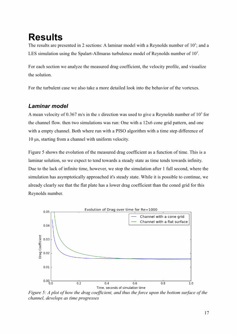
A mean velocity of 0.367 m/s in the x direction was used to give a Reynolds number of 103 for

the channel flow. then two simulations was run: One with a 12x6 cone grid pattern, and one

with a empty channel. Both where run with a PISO algorithm with a time step difference of

10 μs, starting from a channel with uniform velocity.

Figure 5 shows the evolution of the measured drag coefficient as a function of time. This is a

laminar solution, so we expect to tend towards a steady state as time tends towards infinity.

Due to the lack of infinite time, however, we stop the simulation after 1 full second, where the

simulation has asymptotically approached it's steady state. While it is possible to continue, we

already clearly see that the flat plate has a lower drag coefficient than the coned grid for this

Reynolds number.

17

Figure 5: A plot of how the drag coefficient, and thus the force upon the bottom surface of thechannel, develops as time progresses

Figure 6 displays the velocity profile for this solution at the steady state, and the empty

channel's profile is typical for laminar channel flow. We note that the 85 μm cones effectively

limit the velocity around them, and that the typical velocity profile for a laminar channel

develop after they have been passed.

Figure 7 visualize the solution of the coned grid, so that we can better understand it when

compared to the higher Reynolds number solution.

18

Figure 6: The velocity profile of the fully developed laminar flow, read at time = 1s

Turbulent Case

Similar to the previous situation, a mean velocity of 36.7 m/s was used to give a Reynolds

number of 105 for the turbulent channel flow, but this time using a the Spalart-Allmaras

turbulence model. Again two simulations where run: One with the identical 12x6 grid pattern

and one with the empty channel. The mesh was kept identical to the previous set of cases.

Both where run with a PISO algorithm, and for the coned simulation the time-step difference

was 0.1 μs, starting from a channel with uniform velocity. The time step in the empty channel

was increased to 0.5 μs to preserve computational resources.

19

Figure 7: A visualization of laminar flow in a channel with cones. Note that it is turned sideways to save some space.

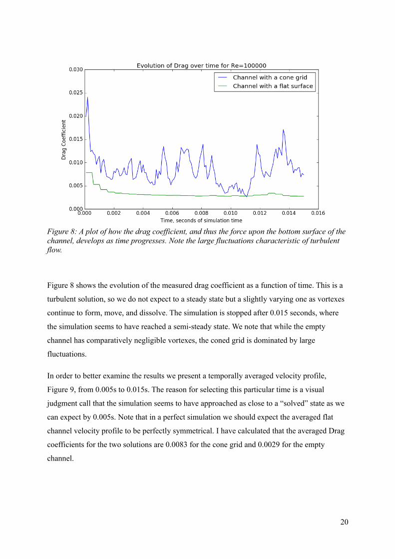
Figure 8 shows the evolution of the measured drag coefficient as a function of time. This is a

turbulent solution, so we do not expect to a steady state but a slightly varying one as vortexes

continue to form, move, and dissolve. The simulation is stopped after 0.015 seconds, where

the simulation seems to have reached a semi-steady state. We note that while the empty

channel has comparatively negligible vortexes, the coned grid is dominated by large

fluctuations.

In order to better examine the results we present a temporally averaged velocity profile,

Figure 9, from 0.005s to 0.015s. The reason for selecting this particular time is a visual

judgment call that the simulation seems to have approached as close to a “solved” state as we

can expect by 0.005s. Note that in a perfect simulation we should expect the averaged flat

channel velocity profile to be perfectly symmetrical. I have calculated that the averaged Drag

coefficients for the two solutions are 0.0083 for the cone grid and 0.0029 for the empty

channel.

20

Figure 8: A plot of how the drag coefficient, and thus the force upon the bottom surface of thechannel, develops as time progresses. Note the large fluctuations characteristic of turbulent flow.

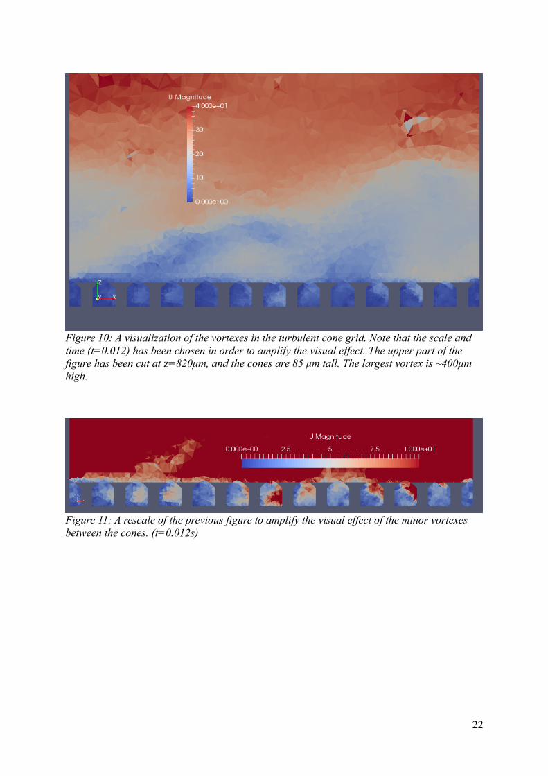
Lastly, we can examine the vortexes visually, in Figure 10. Here we see a snapshot of the

turbulent cone grid solution, with the scale chosen specifically to highlight typical large

vortexes. The largest vortex in the figure is ~400 μm high, and while this fluctuates I wish to

note that I consider it typical, this gives us a characteristic value for the integral length scale,

the scale of the largest vortexes in the system. We will revisit this topic in the next chapter.

Further more we can rescale Figure 10 into Figure 11 to get a better idea about how vortexes

look between the cones. To further examine this, Figure 12 is identical to Figure 11 but simply

moved 60 μm (“half a cone”) in the y direction to see the free flow between the cones. We see

here that the smallest visual vortexes are the ones only a few cells wide. This is to be

expected, as any vortexes smaller than the cells would be impossible to detect. It would also

look like the cones appear to effectively give us two separate systems of vortexes, but we

need to be careful about how much we read into this as the scaling has been selected

specifically to highlight the minor vortexes to the detriment of the largest. As we shall soon

see, this may not be the case.

21

Figure 9: The time averaged velocity profile of the fully developed turbulent flow. The period from t=0.005s to t=0.015s is used for sampling time.

22

Figure 10: A visualization of the vortexes in the turbulent cone grid. Note that the scale and time (t=0.012) has been chosen in order to amplify the visual effect. The upper part of the figure has been cut at z=820μm, and the cones are 85 μm tall. The largest vortex is ~400μm high.

Figure 11: A rescale of the previous figure to amplify the visual effect of the minor vortexes between the cones. (t=0.012s)

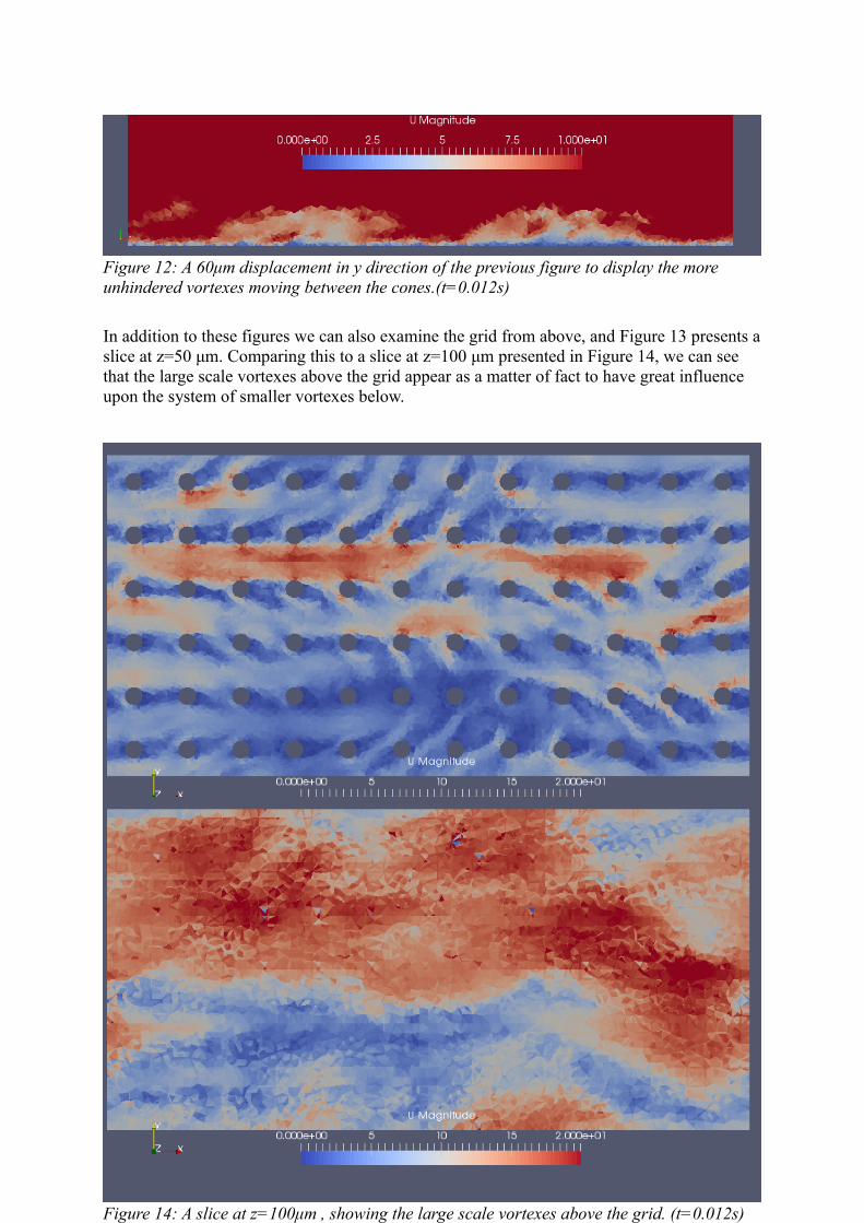
In addition to these figures we can also examine the grid from above, and Figure 13 presents aslice at z=50 μm. Comparing this to a slice at z=100 μm presented in Figure 14, we can see that the large scale vortexes above the grid appear as a matter of fact to have great influence upon the system of smaller vortexes below.

23

Figure 12: A 60μm displacement in y direction of the previous figure to display the more unhindered vortexes moving between the cones.(t=0.012s)

Figure 13: A slice of the cones at z=50 μm, showing a system of vortexes between the cones.(t=0.012s)

Figure 14: A slice at z=100μm , showing the large scale vortexes above the grid. (t=0.012s)

Lastly, I want to display the averaged results in the same manner, to have a good basis for comparison. Figure 16 visualize the velocity over the cones, and Figure 15 show us the average velocity field between them. There is a noteworthy numerical artifact in the upper right corner of Figure 16 that can be compared to Figure 10, and I urge you to keep this in mind when we discuss numerical artefacts in next chapter.

24

Figure 15: A slice of the temporally averaged velocity at z=50 μm.

Figure 16: A temporal average of a vertical slice of the velocity over the cones, showing a height up to z=820μm.

Discussion“Thanks to the development in computer technology it's now possible to get wrong results in

CFD quicker and cheaper than ever before” -Unknown

After having looked at the results in the last section, we will now consider possible error

sources, discuss them, and if possible verify the results with regards to them. The ability to

solve Computational Fluid Dynamic problems is worth little without the ability to also

critically analyze the results.

I've done my very best to minimize all of the effects I describe here, and even if they where to

change the exact answer by some degree, I do not believe they could possibly accumulate,

even together, in large enough quanta to change the final conclusion of this report.

Which is why I remind myself that science cares little for the belief of humans.

Inherent errors from numerical solutions

I assume the reader is knowledgeable about the basic concepts involved in numerical

solutions of equations, and these apply here. Openfoam uses the finite volume method to

approximate the solution to the governing equations, and even without introducing a

turbulence model this would give us errors in the form of computational round-off errors and

errors from the numerical schemes used to approximate the differential terms. This is

especially important when we have a development from a specific initial condition and want

to examine what the end result looks like, as the errors can accumulate over time. In our

situation, however, we have a correcting source term in the momentum equation that will

continually correct the main flow velocity as it approaches a steady state. This correcting term

allow us to neglect any accumulation of computational errors as we steadily approach a

steady-state solution.

Possible errors from basic problem constraints

As we introduce obstacles into a empty channel we do of coarse constrict the flow, increasing

the flow in the center by a unknown amount. In a perfect world we would use a channel of

infinite height, reducing errors from this problem towards zero. However, since that is

unrealistic I was advised by my supervisor Tutkun to keep the possible restriction of the inlet

below 3%. His long experience with simulation suggest that this would keep the error

25

introduced from the obstacle at a negligible level. A secondary issue is the size of the cone

grid, as this possibly restricts the size of the vortexes that can form. I have had to restrain

myself to a 6 x 12 grid, and this is far below the recommendations I have received. A common

practice is to have a channel length ~10 times the height of the channel, and a width equal to

half the length. While the requirement of having a width of half the length is easily

achievable, the length is would require me to use a 250 cone long grid. I estimate this would

take me around 22 years of computation time if I solved for the same amount of time steps.

Since I am using a cyclic boundary condition on the inlet, outlet, and both sides I hope this

does not become a problem, but It is a issue I would have wanted to avoid if I could.

The existence of turbulence in the high Reynolds number case

A possible problem with the LES approach on a unperturbed surface is that under some initial

conditions vortexes might not form at all, giving us a solution comparable to the laminar

result. For our high velocity case with the flat channel this can be a possible issue. We noted

the relative low amount of fluctuations in the drag coefficients development over time in

Figure 8, and while the velocity profile in Figure 9 points to a turbulent flow we should still

verify this further. Figure 17 displays a overhead rendition of the empty channel solution

where the scale is chosen to highlight that vortexes are, indeed, present.

26

Mesh size, and possible impact

A common error source is inadequate refinement of the mesh, or suboptimal distribution of

the cells. In a Large Eddy Simulation like this any vortexes smaller than the cell size in any

point of the simulation will be modeled instead of simulated. Since the smallest cells in the

simulation is placed at the top of the cone and are approximately 5 μm tall, any vortex smaller

than this is modeled. Using the theory of the Kolmogorov Microscales, we can approximate

the smallest vortexes as having a characteristic length of η ~ 0.3 μm, in accordance with

Equation 4 from textbook [6]. η is the length microscale, ν is viscosity for the fluid, U is the

integral velocity and L is the integral length scale. Of coarse refinement of all cells down to

this level would increase the accuracy of the simulation, but unfortunately this would increase

the computational cost, which is already at the “half-to-one-month-of-dedicated-computer-

time” scale and thus can not reasonably be increased for this thesis. My conclusions is thus

based on the assumption that this grid is sufficiently fine to approximate the drag on the

cones, and that any minor vortexes are negligible for the final result.

4) η=(ν

3⋅L

U 3 )(1/4)

=(0.00000113

⋅0.000436.73 )

(1 /4)

=3.2×10−7

Another way to confirm that the mesh is sufficient is is to simply refine the mesh by halving

the length in each dimension and rerunning the simulation. If the new simulation then gives

the same drag coefficient, the solution can be considered mesh independent for this value.

27

Figure 17: A overhead rendition of the turbulent flat plate solution. This is taken 50 μm abovethe flat plate, and clearly visualizes the existence of vortexes in this region.

Unfortunately this would require use of ~8 months of computing time during the end of a 4

month thesis, which is unrealistic with our current understanding of spacetime.

Wallfunction for νt , Spalding

While the instantaneous velocity, pressure, and the transported variable ῦ are all without wall

functions, one is used for the turbulent viscosity νt at the boundary layer of the cones. As such,

I need to evaluate the dimensionless parameter y+, defined by the distance (y), shear velocity

(Ut) and viscosity (ν) of the fluid in Equation 5. Openfoam gives us a tool for calculating the

height of the cell closest to a boundary in y+, and while this value is preferred as small as

possible, it is generally advised to be below 1 by the CFD community for this kind of

simulation. As I validated this value in the end phase of the project, I found that the average

value on the cones at the end time (t=0.015s) was 2.4. The maximum recorded value was 8.8;

and the minimum 0.081. For the flat plate the average value is 3.7; the maximum vale is 6.8;

and the minimum 0.86. I record this as a possible error source, but without further

experiments I can not fully know if it is negligible or not.

5) y+= y

U tν

Turbulence semi-steady-state assumption

In the high velocity case I make the argument, based off the development of the drag

coefficient, that the simulation is as close to a resolved state as I could expect. While I think

this reasoning is sound, the only way to verify this is to apply orders of magnitude more

computational time. If it turns out that the large fluctuations I observed eventually dissipates

and the system reaches a state with less total drag, then my conclusion may need to be

reevaluated. However, considering that the total drag needs to be cut with at least 65% in

order to change my conclusion, I find this unrealistic.

Numerical Artifacts

A unfortunate side effect of using this turbulence model that I could not seem to remove to my

satisfaction was a series of strange numerical artifacts in the middle of the channel, as shown

in Figure 18. While these do not seem to affect any non-negligible vortexes, they do seem to

trow off the middle section slightly. Considering that these give off a noticeable impression in

a large overview look on the channel but does not appear at all close to the area I'm actually

28

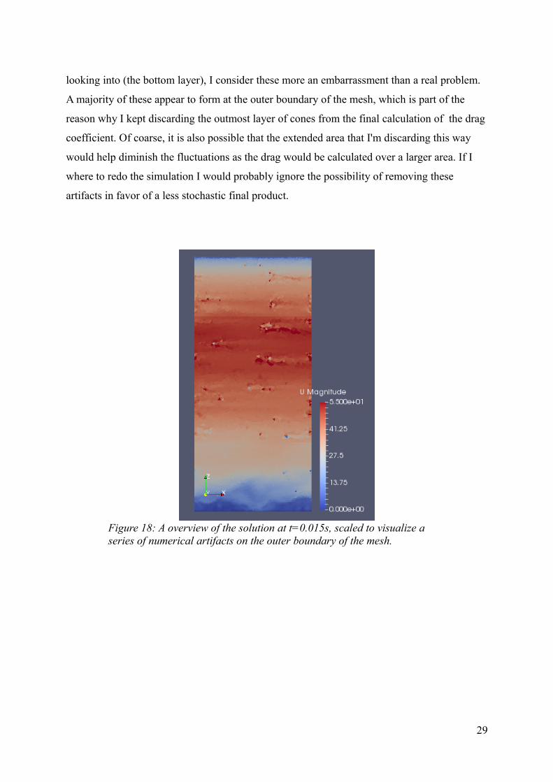
looking into (the bottom layer), I consider these more an embarrassment than a real problem.

A majority of these appear to form at the outer boundary of the mesh, which is part of the

reason why I kept discarding the outmost layer of cones from the final calculation of the drag

coefficient. Of coarse, it is also possible that the extended area that I'm discarding this way

would help diminish the fluctuations as the drag would be calculated over a larger area. If I

where to redo the simulation I would probably ignore the possibility of removing these

artifacts in favor of a less stochastic final product.

29

Figure 18: A overview of the solution at t=0.015s, scaled to visualize a series of numerical artifacts on the outer boundary of the mesh.

ConclusionOur original hypothesis was that a grid of cones could be introduced to a flat plate and that we

would see the total drag force over the area decrease. Unfortunately, the evidence we have

produced showed that adding a cone grid gave an increase in the average drag coefficient by

286%, up from 0.0029 for the empty channel to 0.0083 for the grid. This is, indeed, somewhat

problematic for this hypothesis. It should be noted that there may be a lot to gain from

increasing the domain size, mesh density and simulation time, but this is usually the case for

all CFD projects.

Our hypothesis was based on the work done by Tutkun and his colleges [1], where they had

found positive results. I do therefore want to address this seeming inconsistency between my

work and theirs, and point out that the conclusions are NOT mutually exclusive.

What I have explored is only the effects on a perfectly flat plate, and while I found that the

effects where not beneficial, Tutkun [1] looked at the effect of introducing it at an airfoil, and

how this would affect the boundary layer separation of the flow. I wish to compare this with

the more famous concept of Drag Crisis [7], the phenomena where introducing a roughness

unto a sphere or cylinder, while increasing the local turbulence, decrease the total loss of

energy as the increased turbulence decrease the flow separation and thereby the total wake. If

it was this effect that was observed, and not a effect of the cone grid being better suited than a

flat plate for a plane surface, then both results are not only consistent but supportive of each

other.

I also want to note this flow separation effect only becomes relevant at very specific Reynolds

numbers, for a sphere usually around 105. It is always possible there are beneficial effects that

we did not find because we did not investigate the right flow velocity.

I believe this research has great potential, especially on the subject of wings and other objects

whose wake has a flow separation issue. We may yet learn to re-evaluate what range of grid

systems can be used in such a way and what effects they may have.

From a mechanical engineering point of view, I also want to consider a different issue:

Suppose we DID cover a car with a cone grid like this, and suppose it DID reduce drag

significantly enough to make this worthwhile, we also need to use a grid that is durable as the

car experience common use. A cone only 40 μm wide might be quite fragile, therefore

30

prompting the need to develop more durable grid systems.

On a personal level I must admit that I did not expect these results. It was my hope when I

started this study that I would be able to prove a great potential on flat plates for this

biologically inspired grid, which I suppose remind us why it is always important to approach

a hypothesis with a open mind, and to quantify the results in such a way that our own

preconceptions are rendered mute.

I find it fitting to end the thesis with this quote:

Science is the great antidote to the poison of enthusiasm and superstition. -Adam Smith

31

List of references[1]: S. Dharmarathne, H. B. Evans, A. M. Hamed, B. Aksak, L. P. Chamorro, M. Tutkun, and

L. Castillo (2017): ”Large-scale Motions on a Wind Turbine Airfoil Section”. Submitted to

Journal of Renewable Energy, currently under review for publication.

[2]: Eugene de Villiers (2006): “The Potential of Large Eddy Simulation for the Modeling of

Wall Bounded Flows”. Thesis. Imperial College of London, London, England.

[3]: ESI-OpenCFD (retrieved 21.12.2017): “Numerical Schemes”. Retrieved from

https://www.openfoam.com/documentation/user-guide/fvSchemes.php .

[4]: Hrvoje Jasak (1996): “Error Analysis and Estimation for the Finite Volume Method with

Applications to Fluid Flows”. Thesis. University of London, London, England.

[5]: D. B. Spalding (1961): “A Single Formula for the “Law of the Wall””. Journal of Applied

Mechanics.

[6]: Frank M. White (2006): “Viscous Fluid Flow” (3rd edition), page 400, Singapore,

McGraw-Hill Education.

[7]: National Aeronautics and Space Administration (retrieved 21.12.2017): “Drag of a

Sphere”. Retrieved from https://www.grc.nasa.gov/www/K-12/airplane/dragsphere.html .

32

https://www.grc.nasa.gov/www/K-12/airplane/dragsphere.html

https://www.openfoam.com/documentation/user-guide/fvSchemes.php

Attachments

Script for generating the 6x12 cone grid mesh

As follows I present the script I created for generating a grid mesh. The script can be used as

it is, but note that while most variables in the “control room” segment can be changed at will,

changing the number of cones in the grid will require you to manually update surface loops

that must take these new cones into consideration. These are marked in the script.

//This script is designed to be used with the program GMSH as a .geo file

//The output will be a mesh of a channel with a grid of cones at the bottom.

//It generates a cuboid surrounding each cone, and then adds 3 cuboids on top where cells for the main channel is held.

//The idea is to differentiate cell density depending on the expected boundary thickness.

//Note that if the number of cones are changed, two sections will need to be manually updated, as the surfacefaces of the coneschange.

//Anders Utnes, 2017

//************************************************************

//********************CONTROL ROOM****************************

//Unit of distance is one micrometer

um=0.000001;

//Grid size at different points in mesh

ot= 20*um; //Outer top edge of box surrounding each cone

ol= 10*um; //Outer low edge of box surrounding each cone

il= 10*um; //inner low edge of cone

im= 10*um; //inner middle of each cone, the point of the angle

it= 5*um; //inner top of each cone

bl= 40*um; //The middle part of the boundary layer.

//Dimensions

th= 3000*um; //Channel total height

os= 120*um; //Outer length of the box surrounding cones

oh= 120*um; //Outer height of the box surrounding cones

imh= 65*um; //Height of the cone at the point it starts expanding

ith= 85*um; //Height of the cone at its top

ilr= 20*um; //Radius of the cone at the bottom

imr= 20*um; //Radius of the cone at the point it starts expanding

itr= 42.5*um; //Radius of the cone at the top

33

blt= 700*um; //Expected boundary layer thickness

//Number of cones in x direction

x=12;

//Number of cones in y direction

y=6;

//********REMEMBER TO MANUALLY UPDATE THE SURFACELOOPS*********

//*************************************************************

//Cone and cuboid generation:

//Note that all information relevant to a cone is numbered as such:

//XXYYZZ, where XX refers to the x rank of the cone, YY to the y rank, and ZZ to the point/line/surface variable.

//Initializing wall at x=0:

a=0;

b=0;

Point(10000*a+100*b+0)= {a*os, b*os, 0*oh, ol};

Point(10000*a+100*b+1)= {a*os, b*os, 1*oh, ot};

Line(10000*a+100*b+1)= {10000*a+100*b+0, 10000*a+100*b+1}; //Pillar

For b In {1:y:1}




Line(10000*a+100*b+2)= {10000*a+100*(b-1)+0, 10000*a+100*b+0}; //bot y

Line(10000*a+100*b+3)= {10000*a+100*(b-1)+1, 10000*a+100*b+1}; //top y

Line Loop(10000*a+100*b+1)= {10000*a+100*(b-1)+1, 10000*a+100*b+3, -(10000*a+100*b+1), -(10000*a+100*b+2)};

Plane Surface(10000*a+100*b+1)= {10000*a+100*b+1}; //Side with normal in x direction

EndFor

//Making cones:

For a In {1:x:1}

//Starting on a new wall at y=0

b=0;




Line(10000*a+100*b+4)= {10000*(a-1)+100*b+0, 10000*a+100*b+0}; //bot x

34

Line(10000*a+100*b+5)= {10000*(a-1)+100*b+1, 10000*a+100*b+1}; //top x

Line Loop(10000*a+100*b+2)= {10000*(a-1)+100*b+1, 10000*a+100*b+5, -(10000*a+100*b+1), -(10000*a+100*b+4)};

Plane Surface(10000*a+100*b+2)= {10000*a+100*b+2}; //Side with normal in y direction

For b In {1:y:1}

//Defining a cone:

Point(10000*a+100*b+10)= {(a-0.5)*os-ilr, (b-0.5)*os, 0, il};

Point(10000*a+100*b+11)= {(a-0.5)*os, (b-0.5)*os+ilr, 0, il};

Point(10000*a+100*b+12)= {(a-0.5)*os+ilr, (b-0.5)*os, 0, il};

Point(10000*a+100*b+13)= {(a-0.5)*os, (b-0.5)*os-ilr, 0, il};

Point(10000*a+100*b+14)= {(a-0.5)*os, (b-0.5)*os, 0, il};

Circle(10000*a+100*b+10)= {10000*a+100*b+10, 10000*a+100*b+14, 10000*a+100*b+11};

Circle(10000*a+100*b+11)= {10000*a+100*b+11, 10000*a+100*b+14, 10000*a+100*b+12};

Circle(10000*a+100*b+12)= {10000*a+100*b+12, 10000*a+100*b+14, 10000*a+100*b+13};

Circle(10000*a+100*b+13)= {10000*a+100*b+13, 10000*a+100*b+14, 10000*a+100*b+10};

Line Loop(10000*a+100*b+5)= {10000*a+100*b+10, 10000*a+100*b+11, 10000*a+100*b+12, 10000*a+100*b+13};

Point(10000*a+100*b+20)= {(a-0.5)*os-imr, (b-0.5)*os, imh, il};

Point(10000*a+100*b+21)= {(a-0.5)*os, (b-0.5)*os+imr, imh, il};

Point(10000*a+100*b+22)= {(a-0.5)*os+imr, (b-0.5)*os, imh, il};

Point(10000*a+100*b+23)= {(a-0.5)*os, (b-0.5)*os-imr, imh, il};

Point(10000*a+100*b+24)= {(a-0.5)*os, (b-0.5)*os, imh, il};

Line(10000*a+100*b+20)= {10000*a+100*b+10, 10000*a+100*b+20};

Line(10000*a+100*b+21)= {10000*a+100*b+11, 10000*a+100*b+21};

Line(10000*a+100*b+22)= {10000*a+100*b+12, 10000*a+100*b+22};

Line(10000*a+100*b+23)= {10000*a+100*b+13, 10000*a+100*b+23};

Circle(10000*a+100*b+30)= {10000*a+100*b+20, 10000*a+100*b+24, 10000*a+100*b+21};

Circle(10000*a+100*b+31)= {10000*a+100*b+21, 10000*a+100*b+24, 10000*a+100*b+22};

Circle(10000*a+100*b+32)= {10000*a+100*b+22, 10000*a+100*b+24, 10000*a+100*b+23};

Circle(10000*a+100*b+33)= {10000*a+100*b+23, 10000*a+100*b+24, 10000*a+100*b+20};

Line Loop(10000*a+100*b+10)= {10000*a+100*b+10, 10000*a+100*b+21, -(10000*a+100*b+30), -(10000*a+100*b+20)};




Point(10000*a+100*b+30)= {(a-0.5)*os-itr, (b-0.5)*os, ith, il};

Point(10000*a+100*b+31)= {(a-0.5)*os, (b-0.5)*os+itr, ith, il};

Point(10000*a+100*b+32)= {(a-0.5)*os+itr, (b-0.5)*os, ith, il};

Point(10000*a+100*b+33)= {(a-0.5)*os, (b-0.5)*os-itr, ith, il};

Point(10000*a+100*b+34)= {(a-0.5)*os, (b-0.5)*os, ith, il};

Line(10000*a+100*b+40)= {10000*a+100*b+20, 10000*a+100*b+30};

Line(10000*a+100*b+41)= {10000*a+100*b+21, 10000*a+100*b+31};

Line(10000*a+100*b+42)= {10000*a+100*b+22, 10000*a+100*b+32};

Line(10000*a+100*b+43)= {10000*a+100*b+23, 10000*a+100*b+33};

35

Circle(10000*a+100*b+50)= {10000*a+100*b+30, 10000*a+100*b+34, 10000*a+100*b+31};

Circle(10000*a+100*b+51)= {10000*a+100*b+31, 10000*a+100*b+34, 10000*a+100*b+32};

Circle(10000*a+100*b+52)= {10000*a+100*b+32, 10000*a+100*b+34, 10000*a+100*b+33};

Circle(10000*a+100*b+53)= {10000*a+100*b+33, 10000*a+100*b+34, 10000*a+100*b+30};





Line Loop(10000*a+100*b+30)= {10000*a+100*b+50, 10000*a+100*b+51, 10000*a+100*b+52, 10000*a+100*b+53};

Ruled Surface(10000*a+100*b+10)= {10000*a+100*b+10};








Plane Surface(10000*a+100*b+30)= {10000*a+100*b+30};

//Surrounding the cone with a outer cuboid:




Line(10000*a+100*b+2)= {10000*a+100*(b-1)+0, 10000*a+100*b+0}; //bot y

Line(10000*a+100*b+3)= {10000*a+100*(b-1)+1, 10000*a+100*b+1}; //top y

Line(10000*a+100*b+4)= {10000*(a-1)+100*b+0, 10000*a+100*b+0}; //bot x

Line(10000*a+100*b+5)= {10000*(a-1)+100*b+1, 10000*a+100*b+1}; //top x

Line Loop(10000*a+100*b+1)= {10000*a+100*(b-1)+1, 10000*a+100*b+3, -(10000*a+100*b+1), -(10000*a+100*b+2)};

Line Loop(10000*a+100*b+2)= {10000*(a-1)+100*b+1, 10000*a+100*b+5, -(10000*a+100*b+1), -(10000*a+100*b+4)};

Line Loop(10000*a+100*b+3)= {10000*(a-1)+100*b+2, 10000*a+100*b+4, -(10000*a+100*b+2), -(10000*a+100*(b-1)+4)};

Line Loop(10000*a+100*b+4)= {10000*(a-1)+100*b+3, 10000*a+100*b+5, -(10000*a+100*b+3), -(10000*a+100*(b-1)+5)};

Plane Surface(10000*a+100*b+1)= {10000*a+100*b+1}; //Side with normal in x direction

Plane Surface(10000*a+100*b+2)= {10000*a+100*b+2}; //Side with normal in y direction

Plane Surface(10000*a+100*b+3)= {10000*a+100*b+3, 10000*a+100*b+5}; //Bottom Side with cone intersection removed

Plane Surface(10000*a+100*b+4)= {10000*a+100*b+4}; //Top

Surface Loop(10000*a+100*b+1)= {10000*a+100*b+1, 10000*a+100*b+2, 10000*a+100*b+3, 10000*a+100*b+4, 10000*(a-1)+100*b+1, 10000*a+100*(b-1)+2, 10000*a+100*b+10, 10000*a+100*b+11, 10000*a+100*b+12, 10000*a+100*b+13, 10000*a+100*b+20, 10000*a+100*b+21, 10000*a+100*b+22, 10000*a+100*b+23, 10000*a+100*b+30};

Volume(10000*a+100*b+1)= {10000*a+100*b+1};

EndFor

EndFor

36

//Making the lower part of the channel over the cones:

Point(1000001)= {0, 0, oh+blt, bl};

Point(1000002)= {x*os, 0, oh+blt, bl};

Point(1000003)= {x*os, y*os, oh+blt, bl};

Point(1000004)= {0, y*os, oh+blt, bl};

Line(1000001)= {1, 1000001};

Line(1000002)= {10000*x+1, 1000002};

Line(1000003)= {10000*x+100*y+1, 1000003};

Line(1000004)= {100*y+1, 1000004};

Line(1000011)= {1000001, 1000002};

Line(1000012)= {1000002, 1000003};

Line(1000013)= {1000003, 1000004};

Line(1000014)= {1000004, 1000001};

Line Loop(1000005)= {1000011, 1000012, 1000013, 1000014};

//*************FIRST SECTION THAT NEEDS MANUAL UPDATE*****************

Line Loop(1000001)= { //Top x lines goes here.

10005 ,

20005 ,

30005 ,

40005 ,

50005 ,

60005 ,

70005 ,

80005 ,

90005 ,

100005 ,

110005 ,

120005 ,

1000002, -1000011, -1000001};

Line Loop(1000002)= {//Top y lines goes here.

120103 ,

120203 ,

120303 ,

120403 ,

120503 ,

120603 ,

1000003, -1000012, -1000002};

37

Line Loop(1000003)= { //Top x lines goes here.

10605 ,

20605 ,

30605 ,

40605 ,

50605 ,

60605 ,

70605 ,

80605 ,

90605 ,

100605 ,

110605 ,

120605 ,

1000003, 1000013, -1000004};

Line Loop(1000004)= { //Top y lines goes here.

1000004, 1000014, -1000001,

103 ,

203 ,

303 ,

403 ,

503 ,

603 };

Plane Surface(1000001)= {1000001};

Plane Surface(1000002)= {1000002};

Plane Surface(1000003)= {1000003};

Plane Surface(1000004)= {1000004};

Plane Surface(1000005)= {1000005};

Surface Loop(1000001)= {1000001, 1000002, 1000003, 1000004, 1000005,

10104 ,

10204 ,

10304 ,

10404 ,

10504 ,

10604 ,

20104 ,

20204 ,

20304 ,

20404 ,

20504 ,

20604 ,

30104 ,

38

30204 ,

30304 ,

30404 ,

30504 ,

30604 ,

40104 ,

40204 ,

40304 ,

40404 ,

40504 ,

40604 ,

50104 ,

50204 ,

50304 ,

50404 ,

50504 ,

50604 ,

60104 ,

60204 ,

60304 ,

60404 ,

60504 ,

60604 ,

70104 ,

70204 ,

70304 ,

70404 ,

70504 ,

70604 ,

80104 ,

80204 ,

80304 ,

80404 ,

80504 ,

80604 ,

90104 ,

90204 ,

90304 ,

90404 ,

90504 ,

90604 ,

100104 ,

100204 ,

100304 ,

100404 ,

39

100504 ,

100604 ,

110104 ,

110204 ,

110304 ,

110404 ,

110504 ,

110604 ,

120104 ,

120204 ,

120304 ,

120404 ,

120504 ,

120604 };

//*************END OF FIRST SECTION THAT NEEDS MANUAL UPDATE*****************

Volume(1000001)= {1000001};

//Middle flow

Point(2000001)= {0, 0, th-blt, bl};

Point(2000002)= {x*os, 0, th-blt, bl};

Point(2000003)= {x*os, y*os, th-blt, bl};

Point(2000004)= {0, y*os, th-blt, bl};

Line(2000001)= {1000001, 2000001};

Line(2000002)= {1000002, 2000002};

Line(2000003)= {1000003, 2000003};

Line(2000004)= {1000004, 2000004};

Line(2000011)= {2000001, 2000002};

Line(2000012)= {2000002, 2000003};

Line(2000013)= {2000003, 2000004};

Line(2000014)= {2000004, 2000001};

Line Loop(2000001)= {1000011, 2000002, -2000011, -2000001};

Line Loop(2000002)= {1000012, 2000003, -2000012, -2000002};

Line Loop(2000003)= {-1000013, 2000003, 2000013, -2000004};

Line Loop(2000004)= {2000004, 2000014, -2000001, -1000014};

Line Loop(2000005)= {2000011, 2000012, 2000013, 2000014};

40

Plane Surface(2000001)= {2000001};

Plane Surface(2000002)= {2000002};

Plane Surface(2000003)= {2000003};

Plane Surface(2000004)= {2000004};

Plane Surface(2000005)= {2000005};

Surface Loop(2000001)= {2000001, 2000002, 2000003, 2000004, 2000005, 1000005};

Volume(2000001)= {2000001};

//Upper boundary layer

Point(3000001)= {0, 0, th, ot};

Point(3000002)= {x*os, 0, th, ot};

Point(3000003)= {x*os, y*os, th, ot};

Point(3000004)= {0, y*os, th, ot};

Line(3000001)= {2000001, 3000001};

Line(3000002)= {2000002, 3000002};

Line(3000003)= {2000003, 3000003};

Line(3000004)= {2000004, 3000004};

Line(3000011)= {3000001, 3000002};

Line(3000012)= {3000002, 3000003};

Line(3000013)= {3000003, 3000004};

Line(3000014)= {3000004, 3000001};

Line Loop(3000001)= {2000011, 3000002, -3000011, -3000001};

Line Loop(3000002)= {2000012, 3000003, -3000012, -3000002};

Line Loop(3000003)= {-2000013, 3000003, 3000013, -3000004};

Line Loop(3000004)= {3000004, 3000014, -3000001, -2000014};

Line Loop(3000005)= {3000011, 3000012, 3000013, 3000014};

Plane Surface(3000001)= {3000001};

Plane Surface(3000002)= {3000002};

Plane Surface(3000003)= {3000003};

Plane Surface(3000004)= {3000004};

Plane Surface(3000005)= {3000005};

Surface Loop(3000001)= {3000001, 3000002, 3000003, 3000004, 3000005, 2000005};

Volume(3000001)= {3000001};

41

//*************SECOND SECTION THAT NEEDS MANUAL UPDATE*****************

Physical Surface("inlet")={1000004, 2000004, 3000004,

101 ,

201 ,

301 ,

401 ,

501 ,

601 };

Physical Surface("outlet")={1000002, 2000002, 3000002,

120101 ,

120201 ,

120301 ,

120401 ,

120501 ,

120601 };

Physical Surface("right")={1000001, 2000001, 3000001,

10002 ,

20002 ,

30002 ,

40002 ,

50002 ,

60002 ,

70002 ,

80002 ,

90002 ,

100002 ,

110002 ,

120002 };

Physical Surface("left")={1000003, 2000003, 3000003,

10602 ,

20602 ,

30602 ,

40602 ,

50602 ,

60602 ,

70602 ,

80602 ,

90602 ,

100602 ,

110602 ,

120602 };

42

Physical Surface("top")={3000005};

Physical Surface("ground")={

10103 , 10110 , 10111 , 10112 , 10113 , 10120 , 10121 , 10122 , 10123 , 10130 ,

10203 , 10210 , 10211 , 10212 , 10213 , 10220 , 10221 , 10222 , 10223 , 10230 ,

10303 , 10310 , 10311 , 10312 , 10313 , 10320 , 10321 , 10322 , 10323 , 10330 ,

10403 , 10410 , 10411 , 10412 , 10413 , 10420 , 10421 , 10422 , 10423 , 10430 ,

10503 , 10510 , 10511 , 10512 , 10513 , 10520 , 10521 , 10522 , 10523 , 10530 ,

10603 , 10610 , 10611 , 10612 , 10613 , 10620 , 10621 , 10622 , 10623 , 10630 ,

20103 , 20110 , 20111 , 20112 , 20113 , 20120 , 20121 , 20122 , 20123 , 20130 ,

20603 , 20610 , 20611 , 20612 , 20613 , 20620 , 20621 , 20622 , 20623 , 20630 ,

30103 , 30110 , 30111 , 30112 , 30113 , 30120 , 30121 , 30122 , 30123 , 30130 ,

30603 , 30610 , 30611 , 30612 , 30613 , 30620 , 30621 , 30622 , 30623 , 30630 ,

40103 , 40110 , 40111 , 40112 , 40113 , 40120 , 40121 , 40122 , 40123 , 40130 ,

40603 , 40610 , 40611 , 40612 , 40613 , 40620 , 40621 , 40622 , 40623 , 40630 ,

50103 , 50110 , 50111 , 50112 , 50113 , 50120 , 50121 , 50122 , 50123 , 50130 ,

50603 , 50610 , 50611 , 50612 , 50613 , 50620 , 50621 , 50622 , 50623 , 50630 ,

60103 , 60110 , 60111 , 60112 , 60113 , 60120 , 60121 , 60122 , 60123 , 60130 ,

60603 , 60610 , 60611 , 60612 , 60613 , 60620 , 60621 , 60622 , 60623 , 60630 ,

70103 , 70110 , 70111 , 70112 , 70113 , 70120 , 70121 , 70122 , 70123 , 70130 ,

70603 , 70610 , 70611 , 70612 , 70613 , 70620 , 70621 , 70622 , 70623 , 70630 ,

80103 , 80110 , 80111 , 80112 , 80113 , 80120 , 80121 , 80122 , 80123 , 80130 ,

80603 , 80610 , 80611 , 80612 , 80613 , 80620 , 80621 , 80622 , 80623 , 80630 ,

90103 , 90110 , 90111 , 90112 , 90113 , 90120 , 90121 , 90122 , 90123 , 90130 ,

90603 , 90610 , 90611 , 90612 , 90613 , 90620 , 90621 , 90622 , 90623 , 90630 ,

100103 , 100110 , 100111 , 100112 , 100113 , 100120 , 100121 , 100122 , 100123 , 100130 ,

100603 , 100610 , 100611 , 100612 , 100613 , 100620 , 100621 , 100622 , 100623 , 100630 ,

110103 , 110110 , 110111 , 110112 , 110113 , 110120 , 110121 , 110122 , 110123 , 110130 ,

110603 , 110610 , 110611 , 110612 , 110613 , 110620 , 110621 , 110622 , 110623 , 110630 ,

120103 , 120110 , 120111 , 120112 , 120113 , 120120 , 120121 , 120122 , 120123 , 120130 ,

120203 , 120210 , 120211 , 120212 , 120213 , 120220 , 120221 , 120222 , 120223 , 120230 ,

120303 , 120310 , 120311 , 120312 , 120313 , 120320 , 120321 , 120322 , 120323 , 120330 ,

120403 , 120410 , 120411 , 120412 , 120413 , 120420 , 120421 , 120422 , 120423 , 120430 ,

120503 , 120510 , 120511 , 120512 , 120513 , 120520 , 120521 , 120522 , 120523 , 120530 ,

120603 , 120610 , 120611 , 120612 , 120613 , 120620 , 120621 , 120622 , 120623 , 120630 };

Physical Surface("plate")= {

20203 , 20210 , 20211 , 20212 , 20213 , 20220 , 20221 , 20222 , 20223 , 20230 ,

20303 , 20310 , 20311 , 20312 , 20313 , 20320 , 20321 , 20322 , 20323 , 20330 ,

20403 , 20410 , 20411 , 20412 , 20413 , 20420 , 20421 , 20422 , 20423 , 20430 ,

20503 , 20510 , 20511 , 20512 , 20513 , 20520 , 20521 , 20522 , 20523 , 20530 ,

30203 , 30210 , 30211 , 30212 , 30213 , 30220 , 30221 , 30222 , 30223 , 30230 ,

30303 , 30310 , 30311 , 30312 , 30313 , 30320 , 30321 , 30322 , 30323 , 30330 ,

30403 , 30410 , 30411 , 30412 , 30413 , 30420 , 30421 , 30422 , 30423 , 30430 ,

43

30503 , 30510 , 30511 , 30512 , 30513 , 30520 , 30521 , 30522 , 30523 , 30530 ,

40203 , 40210 , 40211 , 40212 , 40213 , 40220 , 40221 , 40222 , 40223 , 40230 ,

40303 , 40310 , 40311 , 40312 , 40313 , 40320 , 40321 , 40322 , 40323 , 40330 ,

40403 , 40410 , 40411 , 40412 , 40413 , 40420 , 40421 , 40422 , 40423 , 40430 ,

40503 , 40510 , 40511 , 40512 , 40513 , 40520 , 40521 , 40522 , 40523 , 40530 ,

50203 , 50210 , 50211 , 50212 , 50213 , 50220 , 50221 , 50222 , 50223 , 50230 ,

50303 , 50310 , 50311 , 50312 , 50313 , 50320 , 50321 , 50322 , 50323 , 50330 ,

50403 , 50410 , 50411 , 50412 , 50413 , 50420 , 50421 , 50422 , 50423 , 50430 ,

50503 , 50510 , 50511 , 50512 , 50513 , 50520 , 50521 , 50522 , 50523 , 50530 ,

60203 , 60210 , 60211 , 60212 , 60213 , 60220 , 60221 , 60222 , 60223 , 60230 ,

60303 , 60310 , 60311 , 60312 , 60313 , 60320 , 60321 , 60322 , 60323 , 60330 ,

60403 , 60410 , 60411 , 60412 , 60413 , 60420 , 60421 , 60422 , 60423 , 60430 ,

60503 , 60510 , 60511 , 60512 , 60513 , 60520 , 60521 , 60522 , 60523 , 60530 ,

70203 , 70210 , 70211 , 70212 , 70213 , 70220 , 70221 , 70222 , 70223 , 70230 ,

70303 , 70310 , 70311 , 70312 , 70313 , 70320 , 70321 , 70322 , 70323 , 70330 ,

70403 , 70410 , 70411 , 70412 , 70413 , 70420 , 70421 , 70422 , 70423 , 70430 ,

70503 , 70510 , 70511 , 70512 , 70513 , 70520 , 70521 , 70522 , 70523 , 70530 ,

80203 , 80210 , 80211 , 80212 , 80213 , 80220 , 80221 , 80222 , 80223 , 80230 ,

80303 , 80310 , 80311 , 80312 , 80313 , 80320 , 80321 , 80322 , 80323 , 80330 ,

80403 , 80410 , 80411 , 80412 , 80413 , 80420 , 80421 , 80422 , 80423 , 80430 ,

80503 , 80510 , 80511 , 80512 , 80513 , 80520 , 80521 , 80522 , 80523 , 80530 ,

90203 , 90210 , 90211 , 90212 , 90213 , 90220 , 90221 , 90222 , 90223 , 90230 ,

90303 , 90310 , 90311 , 90312 , 90313 , 90320 , 90321 , 90322 , 90323 , 90330 ,

90403 , 90410 , 90411 , 90412 , 90413 , 90420 , 90421 , 90422 , 90423 , 90430 ,

90503 , 90510 , 90511 , 90512 , 90513 , 90520 , 90521 , 90522 , 90523 , 90530 ,

100203 , 100210 , 100211 , 100212 , 100213 , 100220 , 100221 , 100222 , 100223 , 100230 ,

100303 , 100310 , 100311 , 100312 , 100313 , 100320 , 100321 , 100322 , 100323 , 100330 ,

100403 , 100410 , 100411 , 100412 , 100413 , 100420 , 100421 , 100422 , 100423 , 100430 ,

100503 , 100510 , 100511 , 100512 , 100513 , 100520 , 100521 , 100522 , 100523 , 100530 ,

110203 , 110210 , 110211 , 110212 , 110213 , 110220 , 110221 , 110222 , 110223 , 110230 ,

110303 , 110310 , 110311 , 110312 , 110313 , 110320 , 110321 , 110322 , 110323 , 110330 ,

110403 , 110410 , 110411 , 110412 , 110413 , 110420 , 110421 , 110422 , 110423 , 110430 ,

110503 , 110510 , 110511 , 110512 , 110513 , 110520 , 110521 , 110522 , 110523 , 110530 };

Physical Volume("Internal")={1000001, 2000001, 3000001,

10101 ,

10201 ,

10301 ,

10401 ,

10501 ,

10601 ,

20101 ,

44

20201 ,

20301 ,

20401 ,

20501 ,

20601 ,

30101 ,

30201 ,

30301 ,

30401 ,

30501 ,

30601 ,

40101 ,

40201 ,

40301 ,

40401 ,

40501 ,

40601 ,

50101 ,

50201 ,

50301 ,

50401 ,

50501 ,

50601 ,

60101 ,

60201 ,

60301 ,

60401 ,

60501 ,

60601 ,

70101 ,

70201 ,

70301 ,

70401 ,

70501 ,

70601 ,

80101 ,

80201 ,

80301 ,

80401 ,

80501 ,

80601 ,

90101 ,

90201 ,

90301 ,

90401 ,

45

90501 ,

90601 ,

100101 ,

100201 ,

100301 ,

100401 ,

100501 ,

100601 ,

110101 ,

110201 ,

110301 ,

110401 ,

110501 ,

110601 ,

120101 ,

120201 ,

120301 ,

120401 ,

120501 ,

120601 };

//*************END OF SECOND SECTION THAT NEEDS MANUAL UPDATE*****************

46

computational analysis of a drag reducing cone grid

Documents