Continuity of Drag and domain stability in the low Mach number

limits

Eduard Feireisl∗ Elfriede Friedmann†

Institute of Mathematics of the Academy of Sciences of the Czech RepublicZitna 25, 115 67 Praha 1, Czech Republic

Department of Applied MathematicsIm Neuenheimer Feld 293, 69120 Heidelberg, Germany

Abstract

We consider a mathematical model of a rigid body immersed in a viscous, compressible fluidmoving with a velocity prescribed on the boundary of a large channel containing the body. We showcontinuity of the drag functional as well as domain shape stability of solutions in the incompressiblelimit, with the Mach number approaching zero.

Keywords. Navier-Stokes equations, compressible fluids, drag

MSC2010. 35Q30; 76N25

1 Introduction

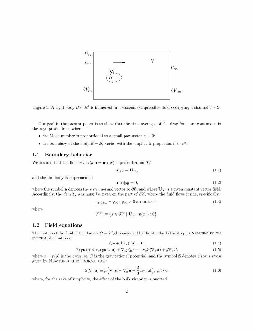
We consider a standard situation frequently studied in fluid mechanics, namely a rigid body B ⊂ R3

immersed in a viscous, compressible fluid occupying a channel Ω = V \ B (Figure 1). The state of thefluid is characterized by the density % = %(t, x) and the velocity field u = u(t, x), the evolution of whichis described by the (barotropic) Navier-Stokes system. The total force imposed by the fluid on the bodyreads ∫

∂BT · n dSx, n -the outer normal vector to ∂B,

whereT = S(∇xu)− p(%)I

is the Cauchy stress tensor, with S the viscous stress and p the pressure. The drag D is defined as thecomponent of this force parallel to the velocity field U∞ imposed on the boundary ∂V :

D =

∫∂B

(S(∇xu) ·U∞ · n− p(%)U∞ · n

)dSx.

∗The work was supported by Grant 201/09/ 0917 of GA CR as a part of the general research programme of the Academyof Sciences of the Czech Republic, Institutional Research Plan AV0Z10190503.†The work was supported by Olympia-Morata-Programme of Heidelberg University.

1

∂Vout

B

V

U∞

U∞

∂Vin

∂B

ρ∞

Figure 1: A rigid body B ⊂ R3 is immersed in a viscous, compressible fluid occupying a channel V \ B.

Our goal in the present paper is to show that the time averages of the drag force are continuous inthe asymptotic limit, where

• the Mach number is proportional to a small parameter ε→ 0;

• the boundary of the body B = Bε varies with the amplitude proportional to εα.

1.1 Boundary behavior

We assume that the fluid velocity u = u(t, x) is prescribed on ∂V ,

u|∂V = U∞, (1.1)

and the the body is impermeableu · n|∂B = 0, (1.2)

where the symbol n denotes the outer normal vector to ∂B, and where U∞ is a given constant vector field.Accordingly, the density % is must be given on the part of ∂V , where the fluid flows inside, specifically,

%|∂Vin= %∞, %∞ > 0 a constant, (1.3)

where∂Vin ≡ x ∈ ∂V | U∞ · n(x) < 0.

1.2 Field equations

The motion of the fluid in the domain Ω = V \B is governed by the standard (barotropic) Navier-Stokessystem of equations:

∂t%+ divx(%u) = 0, (1.4)

∂t(%u) + divx(%u⊗ u) +∇xp(%) = divxS(∇xu) + %∇xG, (1.5)

where p = p(%) is the pressure, G is the gravitational potential, and the symbol S denotes viscous stressgiven by Newton’s rheological law:

S(∇xu) ≡ µ(∇xu +∇Txu−

2

3divxuI

), µ > 0, (1.6)

where, for the sake of simplicity, the effect of the bulk viscosity is omitted.

2

1.3 Slip conditions

We suppose that the tangential component of the velocity satisfies the Navier’s slip boundary con-ditions

[S(∇xu) · n]tan + b[u]tan|∂B = 0, (1.7)

where b ≥ 0 is a friction coefficient. Recently, the possibility of liquid slippage along the boundary hasbeen debated, in particular in connection with nano-technologies, see Priezjev and Troian [13]. Therelevance of the slip condition for gases was discussed by Coron [3], John and Liakos [9], see also Malekand Rajagopal [12].

1.4 Drag

As mentioned above, the total force imposed by the fluid on the body reads∫∂B

T · n dSx,

whereT = S(∇xu)− p(%)I

is the Cauchy stress tensor. The drag D is defined as the component of this force parallel to the velocityU∞:

D =

∫∂B

(S(∇xu) ·U∞ · n− p(%)U∞ · n

)dSx. (1.8)

In addition, we introduce the time averages

Dτ =

∫ τ

0

∫∂B

(S(∇xu) ·U∞ · n− p(%)U∞ · n

)dSx dt.

1.5 Scaling

We suppose that the velocity as well as viscosity are small of order ε, and we neglect the influence of thegravitational force. Thus scaling time as t ≈ t

ε and replacing u ≈ uε , µ ≈ µ

ε we arrive at the system

∂t%+ divx(%u) = 0, (1.9)

∂t(%u) + divx(%u⊗ u) +1

ε2∇xp(%) = divxS(∇xu), (1.10)

where the parameter ε is termed Mach number.We allow the shape of the rigid body to change with ε. More specifically, we are interested in bodies

with “rough boundaries”, with an amplitude proportional to εα and a frequency approaching ε−α, α > 0,(Figure 2). Accordingly, we consider a family of compact sets Bεε>0 enjoying the following properties:

• Bε ⊂ R3 are compact sets Bε ⊂ Br ≡ |x| < r for all ε > 0; (1.11)

• ∂Bε is regular of class C2 for any fixed ε > 0; (1.12)

• Bε satisfy a uniform δ − cone condition, with δ > 0 independent of ε, (1.13)

see Henrot and Pierre [8, Definition 2.4.1];

3

∼ εα

Bε

Figure 2: The body Bεε>0 with “rough boundary” that oscillate with an amplitude proportional to εα

and a frequency approaching ε−α, α > 0.

Bint

rε

rε

Bε

Bext

Figure 3: The boundary of our oscillating body Bε should fulfill the uniform C2-domain condition from[4].

• for each x ∈ ∂Bε, there exists two open balls Bint, Bext of radius rε ≥ εα (Figure 3) such that

Bint ⊂ int[Bε], Bext ⊂ R3 \ Bε, Bint ∩Bext = x. (1.14)

Note that condition (1.14) is chosen in the spirit of Farwig, Kozono, and Sohr [4]. More specifically,the scaled domains 1/εαΩε are the uniform C2-domains discussed in [4].

In addition to the previous hypotheses, we assume, following [2], that the boundaries ∂Bε “oscillate”as ε→ 0, mimicking the effect of “roughness”, see the following section.

Finally, we suppose that the boundary of the channel is “far” from the rigid body. Accordingly, wereplace V by Vε and suppose that

εdist[x, ∂Vε]→∞ as ε→ 0 for any x ∈ Bε. (1.15)

As a consequnce of (1.15), the acoustic waves, propagating at the speed proportional 1/ε, cannot leave acompact subset of Ωε, reach the outer boundary ∂Vε and return in a finite lap of time T . Thus solutionsof the problem behave essentially as those defined on an exterior domain R3 \ Bε, see Section 4.1.

1.6 Domain convergence

A family of domains Ωε = Vε \ Bε satisfying (1.11 - 1.14) enjoys the following properties:

4

• Uniform extension property (see Jones [10, Theorem 1]): There exists an extension operatorE : W 1,p(Ωε)→W 1,p(R3), 1 < p <∞, such that E(v)|Ωε = v,

‖E[v]‖W 1,p(R3) ≤ c‖v‖W 1,p(Ωε),

with the constant c independent of ε.

• Uniform Korn’s inequality (see [1, Proposition 4.1]):

Let v ∈ W 1,2(Ωε ∩ B;R3), where B is an open ball of radius R, and M ⊂ Ωε ∩ B such that|M | > m > 0. Then

‖v‖2W 1,2(Ωε∩B;R3) ≤ c(m,R)

(∥∥∥∥∇xv +∇txv −2

3divxvI

∥∥∥∥2

L2(Ωε∩B;R3×3)

+

∫M

|v|2 dx

), (1.16)

with c(m) independent of ε→ 0.

• Compactness (see Henrot and Pierre [8, Theorem 2.4.10]): There exists a compact set B satisfyingthe uniform δ−cone condition, and a suitable subsequence of ε′s (not relabeled) such that

|Bε \ B|+ |B \ Bε| → 0 as ε→ 0. (1.17)

For each x0 ∈ ∂B, there is xε,0 ∈ ∂Bε such that xε,0 → x0, in particular,

B ⊂ Br. (1.18)

For any compact K ⊂ R3 \ B, there exists ε(K) such that

K ⊂ R3 \ Bε for all ε < ε(K). (1.19)

• Roughness (see [2]): The limit obstacle B is Lipschitz, in particular almost any point y ∈ ∂B(in the sense of the 2-D Hausdorff measure) admits an (outer) normal vector ny. We require theboundaries ∂Bε to oscillate in the following sense:

limr→0

(lim infε→0

1

|∂Bε ∩Br(y)|2

∫∂Bε∩Br(y)

|n ·w| dSx

)> 0 for any |w| = 1, w · ny = 0, (1.20)

where Br(y) denotes the ball of radius r centered at y, cf. [2, Corollary 4.4].

We setΩ = R3 \ B.

1.7 Energy balance and ill-prepared initial data

We start by introducing an auxiliary function u∞ ∈W 1,∞(R3) such that

u∞(x) = 0 for x ∈ B2r,u∞(x) = U∞ for x ∈ R3 \B3r, divxu∞ = 0 for a.a. x ∈ R3, (1.21)

where the parameter r > 0 is the same as in (1.11).

5

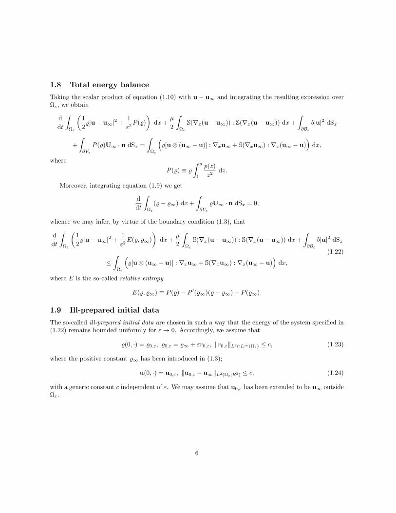
1.8 Total energy balance

Taking the scalar product of equation (1.10) with u − u∞ and integrating the resulting expression overΩε, we obtain

d

dt

∫Ωε

(1

2%|u− u∞|2 +

1

ε2P (%)

)dx+

µ

2

∫Ωε

S(∇x(u− u∞)) : S(∇x(u− u∞)) dx+

∫∂Bε

b|u|2 dSx

+

∫∂Vε

P (%)U∞ · n dSx =

∫Ωε

(%[u⊗ (u∞ − u)] : ∇xu∞ + S(∇xu∞) : ∇x(u∞ − u)

)dx,

where

P (%) ≡ %∫ %

1

p(z)

z2dz.

Moreover, integrating equation (1.9) we get

d

dt

∫Ωε

(%− %∞) dx+

∫∂Vε

%U∞ · n dSx = 0;

whence we may infer, by virtue of the boundary condition (1.3), that

d

dt

∫Ωε

(1

2%|u− u∞|2 +

1

ε2E(%, %∞)

)dx+

µ

2

∫Ωε

S(∇x(u− u∞)) : S(∇x(u− u∞)) dx+

∫∂Bε

b|u|2 dSx

(1.22)

≤∫

Ωε

(%[u⊗ (u∞ − u)] : ∇xu∞ + S(∇xu∞) : ∇x(u∞ − u)

)dx,

where E is the so-called relative entropy

E(%, %∞) ≡ P (%)− P ′(%∞)(%− %∞)− P (%∞).

1.9 Ill-prepared initial data

The so-called ill-prepared initial data are chosen in such a way that the energy of the system specified in(1.22) remains bounded uniformly for ε→ 0. Accordingly, we assume that

%(0, ·) = %0,ε, %0,ε = %∞ + εr0,ε, ‖r0,ε‖L2∩L∞(Ωε) ≤ c, (1.23)

where the positive constant %∞ has been introduced in (1.3);

u(0, ·) = u0,ε, ‖u0,ε − u∞‖L2(Ωε;R3) ≤ c, (1.24)

with a generic constant c independent of ε. We may assume that u0,ε has been extended to be u∞ outsideΩε.

6

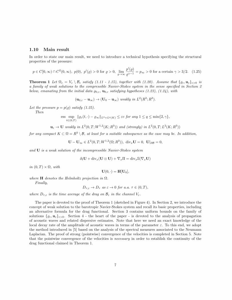
1.10 Main result

In order to state our main result, we need to introduce a technical hypothesis specifying the structuralproperties of the pressure:

p ∈ C[0,∞) ∩ C2(0,∞), p(0), p′(%) > 0 for % > 0, lim%→∞

p′(%)

%γ−1= p∞ > 0 for a certain γ > 3/2. (1.25)

Theorem 1 Let Ωε = Vε \ Bε satisfy (1.11 - 1.15), together with (1.20). Assume that %ε,uεε>0 isa family of weak solutions to the compressible Navier-Stokes system in the sense specified in Section 2below, emanating from the initial data %0,ε, u0,ε satisfying hypotheses (1.23), (1.24), with

(u0,ε − u∞)→ (U0 − u∞) weakly in L2(R3;R3).

Let the pressure p = p(%) satisfy (1.25).Then

ess supt∈(0,T )

‖%ε(t, ·)− %∞‖L2+Lq(K) ≤ εc for any 1 ≤ q ≤ min2, γ,

uε → U weakly in L2(0, T ;W 1,2(K;R3)) and (strongly) in L2(0, T ;L2(K;R3))

for any compact K ⊂ Ω = R3 \ B, at least for a suitable subsequence as the case may be. In addition,

U−U∞ ∈ L2(0, T ;W 1,2(Ω;R3)), divxU = 0, U|∂B = 0,

and U is a weak solution of the incompressible Navier-Stokes system

∂tU + divx(U⊗U) +∇xΠ = divxS(∇xU)

in (0, T )× Ω, withU(0, ·) = H[U0],

where H denotes the Helmholtz projection in Ω.Finally,

Dτ,ε → Dτ as ε→ 0 for a.a. τ ∈ (0, T ),

where Dτ,ε is the time average of the drag on Bε in the channel Vε.

The paper is devoted to the proof of Theorem 1 (sketched in Figure 4). In Section 2, we introduce theconcept of weak solution to the barotropic Navier-Stokes system and recall its basic properties, includingan alternative formula for the drag functional. Section 3 contains uniform bounds on the family ofsolutions %ε,uεε>0. Section 4 - the heart of the paper - is devoted to the analysis of propagationof acoustic waves and related dispersive estimates. Note that here we need an exact knowledge of thelocal decay rate of the amplitude of acoustic waves in terms of the parameter ε. To this end, we adoptthe method introduced in [5] based on the analysis of the spectral measures associated to the NeumannLaplacian. The proof of strong (pointwise) convergence of the velocities is completed in Section 5. Notethat the pointwise convergence of the velocities is necessary in order to establish the continuity of thedrag functional claimed in Theorem 1.

7

uε

∂Vε

slip no-slip

U

Vε

B

ε→ 0

Bε

Figure 4: The limit process of compressible Navier-Stokes flow with slip boundary condition on a rigidbody with oscillating boundary Bε in the domain V ε \ Bε to incompressible Navier-Stokes flow with noslip condition on the smooth domain B in the exterior domain Ω \ B. The timeaveraged drag Dτ,ε on Bεconverges continuously to the drag Dτ on B.

2 Weak formulation

In this section, we introduce the concept of weak solution to the compressible Navier-Stokes system. Notethat existence of global-in-time weak solution, under hypothesis (1.25), can be proved by the methodsdeveloped by Lions [11] and [7].

2.1 Weak solutions to the compressible Navier-Stokes system

We shall say that %ε, uε is a weak solution of the Navier-Stokes system (1.9), (1.10), supplemented withthe boundary conditions (1.1 - 1.3), (1.7), and the initial conditions (1.23), (1.24) if:

• the quantities %ε, uε belong to the following regularity class: %ε ∈ Cweak([0, T ];Lγ(Ωε)) for a certainγ > 3/2, (uε − u∞) ∈ L2(0, T ;W 1,2

0 (Ωε;R3)), p(%ε) ∈ L1((0, T )× Ωε);

• Equation of continuity (1.4), together with (1.1 - 1.3), (1.9) is satisfied in the sense of distri-butions, specifically,∫ T

0

∫Ωε

(%ε∂tϕ+ %εuε · ∇xϕ) dx dt = −∫

Ωε

%0,εϕ(0, ·) dx+

∫ T

0

∫∂Vin,ε

%∞U∞ · n dSxϕ dt (2.1)

holds for any ϕ ∈ C∞c ([0, T )× Ωε ∪ ∂Vin,ε);

• Momentum equation (1.10), with (1.7), (1.24) is replaced by a family of integral identities∫ T

0

∫Ωε

(%εuε · ∂tϕ+ %ε(uε ⊗ uε) : ∇xϕ+

1

ε2p(%ε)divxϕ

)dx dt (2.2)

8

=

∫ T

0

∫Ωε

S(∇xuε) : ∇xϕ dx dt−∫ T

0

∫∂Bε

buε · ϕ dSx dt−∫

Ωε

%0,εu0,ε · ϕ(0, ·) dx

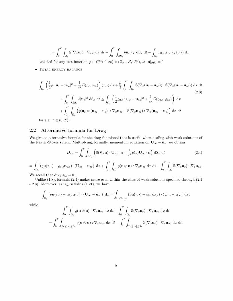
satisfied for any test function ϕ ∈ C∞c ([0,∞)× (Ωε ∪ Bε;R3), ϕ · n|∂Bε = 0;

• Total energy balance

∫Ωε

(1

2%ε|uε − u∞|2 +

1

ε2E(%ε, %∞)

)(τ, ·) dx+

µ

2

∫ τ

0

∫Ωε

S(∇x(uε−u∞)) : S(∇x(uε−u∞)) dx dt

(2.3)

+

∫ τ

0

∫∂Bε

b|uε|2 dSx dt ≤∫

Ωε

(1

2%0,ε|u0,ε − u∞|2 +

1

ε2E(%0,ε, %∞)

)dx

+

∫ τ

0

∫Ωε

(%[uε ⊗ (u∞ − uε)] : ∇xu∞ + S(∇xu∞) : ∇x(u∞ − uε)

)dx dt

for a.a. τ ∈ (0, T ).

2.2 Alternative formula for Drag

We give an alternative formula for the drag functional that is useful when dealing with weak solutions ofthe Navier-Stokes sytem. Multiplying, formally, momentum equation on U∞ − u∞ we obtain

Dτ,ε =

∫ τ

0

∫∂Bε

(S(∇xu) ·U∞ · n−

1

ε2p(%)U∞ · n

)dSx dt (2.4)

=

∫Ωε

(%u(τ, ·)− %0,εu0,ε) · (U∞ − u∞) dx+

∫ τ

0

∫Ωε

%(u⊗u) : ∇xu∞ dx dt−∫ τ

0

∫Ωε

S(∇xuε) : ∇xu∞.

We recall that divxu∞ = 0.Unlike (1.8), formula (2.4) makes sense even within the class of weak solutions specified through (2.1

- 2.3). Moreover, as u∞ satisfies (1.21), we have∫Ωε

(%u(τ, ·)− %0,εu0,ε) · (U∞ − u∞) dx =

∫Ωε∩B3r

(%u(τ, ·)− %0,εu0,ε) · (U∞ − u∞) dx,

while ∫ τ

0

∫Ωε

%(u⊗ u) : ∇xu∞ dx dt−∫ τ

0

∫Ωε

S(∇xuε) : ∇xu∞ dx dt

=

∫ τ

0

∫2r≤|x|≤3r

%(u⊗ u) : ∇xu∞ dx dt−∫ τ

0

∫2r≤|x|≤3r

S(∇xuε) : ∇xu∞ dx dt.

9

3 Uniform bounds

Similarly to [6, Chapter 4], it is convenient to introduce the essential and residual components of afunction h as

h = [h]ess + [h]res, [h]ess = χ(%ε)h, [h]res = (1− χ(%ε))h,

where χ ∈ C∞c (0,∞),

0 ≤ χ ≤ 1, supp[χ] ⊂ [%∞/4, 4%∞], %|[%∞/2,2%∞] = 1.

As will become clear from the uniform bounds derived below, it is the essential part that contains theinformation about the limit system while the residual component vanishes in the asymptotic limit ε→ 0.

3.1 Bounds based on energy estimates

The energy balance (2.3), together with the restrictions (1.23), (1.24) imposed on the initial data, providesthe uniform bounds necessary for performing the asymptotic limit. First, observe that∫

Ωε

(1

2%0,ε|u0,ε − u∞|2 +

1

ε2E(%0,ε, %∞)

)dx ≤ c uniformly for ε→ 0 (3.1)

as a direct consequence of (1.23), (1.24).Moreover, as the function u∞ satisfies (1.21), we get∣∣∣∣∫

Ωε

%[uε ⊗ (u∞ − uε)] : ∇xu∞ dx

∣∣∣∣ ≤ c∫2r≤|x|≤3r

%ε(1 + |uε − u∞|2

)dx, (3.2)

while, by the same token,∣∣∣∣∫Ωε

S(∇xu∞) : ∇x(u∞ − uε) dx

∣∣∣∣ ≤ c(δ) + δ

∫2r≤|x|≤3r

|S(∇x(uε − u∞))|2 dx for any δ > 0. (3.3)

On the other hand, the relative entropy E(%, %∞) is a strictly convex function of % attaining its globalminimum (zero) at %∞. Furthermore, in accordance with hypothesis (1.25), we have

1

ε2E(%, %∞) ≥ c

([%− %∞

ε

]2

ess

+

[1 +

%γ

ε2

]res

), c > 0. (3.4)

Summing up (1.25 - 3.4) we use the energy inequality (2.3) to obtain

ess supt∈(0,T )

∥∥∥∥[%ε − %∞ε

]ess

∥∥∥∥L2(Ωε)

≤ c, (3.5)

ess supt∈(0,T )

∥∥∥∥[%ε − %∞ε

]res

∥∥∥∥Lq(Ωε)

≤ ε2−qq c(q) for all 1 ≤ q ≤ minγ, 2, (3.6)

ess supt∈(0,T )

‖1ess‖L1(Ωε) ≤ ε2c, (3.7)

10

ess supt∈(0,T )

‖√%ε(uε − u∞)‖L2(Ωε;R3) ≤ c, (3.8)

and ∫ T

0

∫Ωε

|S(∇x(uε − u∞))|2 dx dt ≤ c. (3.9)

Finally, combining (3.7 - 3.9) with a variant of Korn’s inequality (1.16) we conclude that∫ T

0

‖uε − u∞‖2W 1,2(Ωε;R3) dt ≤ c. (3.10)

3.2 Convergence

In accordance with the discussion in Section 1.5, the limit physical space can be identified as the exteriordomain

Ω = R3 \ B,

where Bε → B in the sense of (1.17 - 1.19). It follows from the uniform bounds (3.5 - 3.10) that

ess supt∈(0,T )

‖%ε − %∞‖L2+Lq(K) ≤ εc for any 1 ≤ q ≤ min 2γ, (3.11)

uε → U weakly in L2(0, T ;W 1,2(K;R3)) (3.12)

for any compact K ⊂ Ω, at least for a suitable subsequence as the case may be. Here, in addition,

U−U∞ ∈ L2(0, T,W 1,2(Ω;R3)), (3.13)

and, letting ε→ 0 in the equation of continuity (2.1), we deduce that

divxU = 0 a.a. in (0, T )× Ω. (3.14)

Moreover, since the boundaries ∂Bε oscillate as stated in (1.20), we can use [2, Theorem 4.1, Corollary4.4] to deduce that the limit velocity field satisfies the no-slip boundary condition

U|∂B = 0. (3.15)

Finally, taking ϕ ∈ C∞c ([0, T )×Ω;R3), divxϕ = 0 as a test function in the momentum equation (2.2)and letting ε→∞ we may infer that∫ T

0

∫Ω

(%∞U · ∂tϕ+ (%U⊗U) : ∇xϕ

)dx dt (3.16)

=

∫ T

0

∫Ω

S(∇xU) : ∇xϕ dx dt−∫

Ω

%∞u0 · ϕ(0, ·) dx,

where the symbol %U⊗U stands for a weak limit of %εuε ⊗ uε.Consequently, we have to show

%U⊗U = %U⊗U,

11

which clearly follows from the strong (a.a. pointwise) convergence of the velocities claimed in Theorem1. To this end, we first observe that

t 7→∫

Ω

%εuε · ϕ dx

→t 7→ %∞

∫Ω

U · ϕ dx

in C[0, T ] for any ϕ ∈ C∞c (Ω;R3), divxϕ = 0. (3.17)

As the spatial gradients of uε are bounded (see (3.10)), relation (3.17) is enough to deduce strongconvergence of the solenoidal component of the velocities, see Section 5 below. In the remaining part ofthe paper, we show that the gradient part of the velocities, representing acoustic waves, decays to zeroon compact sets as a direct consequence of dispersion. This piece of information will be combined with(3.17) in Section 5 in order to obtain the desired strong convergence of the velocity fields as claimed inTheorem 1.

4 Acoustic waves

We derive an equation describing propagation of acoustic waves and apply the dispersive estimates inorder to deduce a local decay to zero of the acoustic energy.

4.1 Acoustic equation

We write equation (1.9) in the form

ε∂t

(%ε − %∞

ε

)+ divx (%ε(uε − u∞)) = −divx(%εu∞) = −εdivx

(%ε − %∞

εu∞

), (4.1)

and, similarly,

ε∂t (%ε(uε − u∞)) + p′(%∞)∇x(%ε − %∞

ε

)= εu∞divx(%εuε)− εdivx(%εuε ⊗ uε) (4.2)

εdivxS(∇xuε)− ε(

1

ε2∇x (p(%ε)− p′(%∞)(%ε − %∞)− p(%∞))

).

Next, we eliminate the effect of the outer boundary ∂Vε by introducing a cut-off function

ηε ∈ C∞c (R3), 0 ≤ ηε ≤ 1, ηε|B1/ε= 1, ηε|R3\B2/ε

= 0, |∇xηε| ≤ ε. (4.3)

Accordingly, for

rε ≡ ηε%ε − %∞

ε, Vε = ηε%ε(uε − u∞),

we haveε∂trε + divxVε = F 1

ε , (4.4)

ε∂tVε + p′(%∞)∇xrε = F2ε, (4.5)

where

F 1ε = %ε∇xηε · (uε − u∞) + εηεdivx

(%ε − %∞

εu∞

), (4.6)

12

and

F2ε = ∇xηε

(%ε − %∞

ε

)+ εηεu∞divx(%εuε)− εηεdivx(%εuε ⊗ uε) (4.7)

+εηεdivxS(∇xuε)− ε(ηεε2∇x (p(%ε)− p′(%∞)(%ε − %∞)− p(%∞))

).

Equations (4.4), (4.5) are understood in the weak sense in the set R3 \ Bε. To simplify notation, weset Ωε = R3 \ Bε in the remaining part of the paper. Accordingly, equation (4.4) is replaced by a familyof integral identities∫ T

0

∫Ωε

(εrε∂tϕ+ Vε · ∇xϕ) dx dt = −∫

Ωε

εηεr0,εϕ(0, ·) dx−∫ T

0

∫Ωε

(%ε∇xηε · (uε − u∞)ϕ) dx dt

(4.8)

+

∫ T

0

∫Ωε

ε%ε − %∞

εu∞ · ∇x(ηεϕ) dx dt

for any test function ϕ ∈ C∞c ([0, T )× Ωε), while (4.5) reads∫ T

0

∫Ωε

(εVε · ∂tϕ+ p′(%∞)rεdivxϕ) dx dt = −∫

Ωε

εV0,ε · ϕ(0, ·) dx (4.9)

=

∫ T

0

∫Ωε

(ε%ε∇x(ηεu∞ · ϕ) · uε −∇xηε · ϕ

(%ε − %∞

ε

)+ ε(%εuε ⊗ uε) : ∇x(ηεϕ)

)dxdt

+

∫ T

0

∫Ωε

(εS(∇xuε) : ∇x(ηεϕ) + εdivx(ηεϕ)

1

ε2

(p(%ε)− p′(%∞)(%ε − %∞)− p(%∞)

))dx dt

−∫ T

0

∫∂Bε

εbηεuε · ϕ dSx dt

for any ϕ ∈ C∞c ([0,∞)× Ωε;R3), ϕ · n|∂Bε = 0.

4.2 Helmholtz projection - acoustic wave equation

We write Vε asVε = Hε[Vε] +∇xΨε,

where Hε denotes the standard Helmholtz projection in Ωε. We have

Vε = [ηε%ε(uε − u∞)]ess + [ηε%ε(uε − u∞)]res,

where, by virtue of the uniform estimates (3.6), (3.8)

ess supt∈(0,T )

‖[ηε%ε(uε − u∞)]ess‖L2(Ωε;R3) ≤ c, (4.10)

and

ess supt∈(0,T )

‖[ηε%ε(uε − u∞)]res‖Ls(Ωε;R3) ≤ ε1/γc, s =

2γ

γ + 2. (4.11)

13

Consequently, the acoustic potential Ψε, ∇xΨε = H⊥ε [Vε] is determined as the unique solution to theproblem

∆Ψε = divxVε in Ωε, (∇xΨε −Vε) · n|∂Ωε= 0, Ψε ∈ D1,2 +D1,s(Ωε),

where s is the same as in (4.11). More precisely, we have

∇xΨε = H⊥ε [[Vε]ess] + H⊥ε [[Vε]res], (4.12)

where, in accordance with (4.10),

ess supt∈(0,T )

‖H⊥ε [[Vε]ess]‖L2(Ωε) ≤ c uniformly for ε→ 0. (4.13)

We recall that Helmholtz projection is bounded in L2(Ωε;R3), uniformly for ε→ 0.

Denoting ∆N,ε the Neumann Laplacian in Ωε, we may use the quantities ∇x∆−1N,εϕ as test function

in (4.9) to rewrite system (4.8), (4.9) in the form∫ T

0

∫Ωε

(εrε∂tϕ+∇xΨε · ∇xϕ) dx dt = −∫

Ωε

εηεr0,εϕ(0, ·) dx−∫ T

0

∫Ωε

(%ε∇xηε · (uε − u∞)ϕ) dx dt

(4.14)

+

∫ T

0

∫Ωε

ε%ε − %∞

εu∞ · ∇x(ηεϕ) dx dt

for any test function ϕ ∈ C∞c ([0, T )× Ωε),∫ T

0

∫Ωε

(−εΨε∂tϕ+ p′(%∞)rεϕ) dx dt =

∫Ωε

εΨ0,εϕ(0, ·) dx (4.15)

=

∫ T

0

∫Ωε

(ε%ε∇x(ηεu∞ · ∇x∆−1

N,ε[ϕ]) · uε −∇xηε · ∇x∆−1N,ε[ϕ]

(%ε − %∞

ε

))dx dt

+

∫ T

0

∫Ωε

ε(%εuε ⊗ uε) : ∇x(ηε∇x∆−1N,ε[ϕ]) dxdt

+

∫ T

0

∫Ωε

εS(∇xuε) : ∇x(ηε∇x∆−1N,ε[ϕ]) dx dt

+

∫ T

0

∫Ωε

(εdivx(ηε∇x∆−1

N,ε[ϕ])1

ε2

(p(%ε)− p′(%∞)(%ε − %∞)− p(%∞)

))dx dt

−∫ T

0

∫∂Bε

εbηεuε · ∇x∆−1N,ε[ϕ] dSx dt

for any ϕ ∈ C∞c ([0,∞)× Ωε).

14

4.3 Uniform estimates

The operator −∆N,ε can be viewed as a non-negative self-adjoint operator on the Hilbert space L2(Ωε),with a domain of definition

D(∆N,ε) =v ∈W 1,2(Ωε)

∣∣∣ there exists g ∈ L2(Ωε) such that∫Ωε

∇xv · ∇xϕ dx =

∫Ωε

gϕ dx for all ϕ ∈W 1,2(Ωε)

.

Our aim is to write all forcing terms in system (4.14), (4.15) in the form G(−∆N,ε)[hε], where G is a(smooth) function defined on (0,∞) and hε ∈ L2(0, T ;L2(Ωε)). To this end, we use the uniform boundsestablished in Section 3:

1. In accordance with (4.3),

|%ε∇xηε · (uε − u∞)| ≤ ε|%ε(uε − u∞)|,

where, by virtue of (4.10), (4.11)

ess supt∈(0,T )

‖%ε(uε − u∞)‖L2+Ls(Ωε;R3) ≤ c, s =2γ

γ + 2> 6/5,

uniformly for ε→ 0.

2. Similarly, as a direct consequence of (3.5), (3.6),

ess supt∈(0,T )

∥∥∥∥%ε − %∞εu∞

∥∥∥∥L2+Lq(Ωε;R3)

≤ c, 1 ≤ q ≤ minγ, 2.

In view of the previous estimates, equation (4.14) can be written in the form

ε∂trε + ∆N,εΨε = εG1ε, rε(0, ·) = ηεr0,ε, (4.16)

with‖ηεr0,ε‖L2(Ωε) ≤ c, (4.17)

ess supt∈(0,T )

∣∣(G1ε(t, ·)|ϕ

)∣∣ ≤ c‖ϕ‖W 1,2∩W 1,6(Ωε). (4.18)

Analogously, the forcing terms in (4.15) can be estimated as follows:

1. We have∇xΨ0,ε = H⊥ε [ηε%0,ε(u0,ε − u∞)];

whence‖Ψ0,ε‖D1,2(Ωε) = ‖(−∆N,ε)

1,2Ψ0,ε‖L2(Ωε) ≤ c.

15

2. By virtue of (3.6 - 3.8),

ess supt∈(0,T )

‖%εuε‖L2+Ls(Ωε) ≤ c, s =2γ

γ + 1> 6/5;

thereforeess sup

t∈(0,T )

∥∥∥%ε∇x(ηεu∞ · ∇x∆−1N,ε[ϕ]) · uε

∥∥∥L1(Ωε)

≤ c(∥∥∇2

x(−∆N,ε)−1[ϕ]

∥∥L2∩L6(Ωε)

+∥∥∇x(−∆N,ε)

−1[ϕ]∥∥L2∩L6(Ωε;R3)

).

Noticing that∥∥∇x(−∆N,ε)−1[ϕ]

∥∥L6(Ωε;R3)

≤ c∥∥∇2

x(−∆N,ε)−1[ϕ]

∥∥L2(Ωε)

uniformly for ε→ 0,

we concludeess sup

t∈(0,T )

∥∥∥%ε∇x(ηεu∞ · ∇x∆−1N,ε[ϕ]) · uε

∥∥∥L1(Ωε)

≤ c(∥∥∇2

x(−∆N,ε)−1[ϕ]

∥∥L2∩L6(Ωε)

+∥∥∥(−∆N,ε)

−1/2[ϕ]∥∥∥L2(Ωε)

).

3. Using estimates (3.5), (3.6), we have

ess supt∈(0,T )

∥∥∥∥∇xηε %ε − %∞ε

∥∥∥∥L2+Lq(Ωε)

≤ εc, 1 ≤ q ≤ minγ, 2;

whence

ess supt∈(0,T )

∥∥∥∥∇xηε · ∇x∆−1N,ε[ϕ]

(%ε − %∞

ε

)∥∥∥∥L1(Ωε)

≤ εc∥∥∥∇x∆−1

N,ε[ϕ]∥∥∥L2∩L6(Ωε)

≤ ε(∥∥∥(−∆N,ε)

−1/2[ϕ]∥∥∥L2(Ωε)

+∥∥∇2

x(−∆N,ε)−1[ϕ]

∥∥L2(Ωε)

).

4. Next, we write

%εuε ⊗ uε = %ε(uε − u∞)× (uε − u∞) + %ε(uε − u∞)⊗ u∞ + %εu∞ ⊗ (uε − u∞)

+(%ε − %∞)u∞ ⊗ u∞ + %∞u∞ ⊗ u∞,

where, similarly to Step 2,

ess supt∈(0,T )

∥∥%ε[(uε − u∞)⊗ u∞] : ∇x(ηε∇x(−∆N,ε)

−1[ϕ])∥∥L1(Ωε)

+

ess supt∈(0,T )

∥∥%ε[u∞ ⊗ (uε − u∞)] : ∇x(ηε∇x(−∆N,ε)

−1[ϕ])∥∥L1(Ωε)

≤ c(∥∥∇2

x(−∆N,ε)−1[ϕ]

∥∥L2∩L6(Ωε)

+∥∥∥(−∆N,ε)

−1/2[ϕ]∥∥∥L2(Ωε)

).

16

Moreover, exactly as in Step 3,

ess supt∈(0,T )

∥∥(%ε − %∞)[u∞ ⊗ u∞] : ∇x(ηε∇x(−∆N,ε)

−1[ϕ])∥∥L1(Ωε)

≤ εc(∥∥∇2

x(−∆N,ε)−1[ϕ]

∥∥L2∩L6(Ωε)

+∥∥∥(−∆N,ε)

−1/2[ϕ]∥∥∥L2(Ωε)

).

Furthermore,%ε(uε − u∞)⊗ (uε − u∞)

=√

[%ε]ess√%ε(uε − u∞)⊗ (uε − u∞) +

√[%ε]res

√%ε(uε − u∞)⊗ (uε − u∞),

where, by virtue of (3.8)∥∥∥√[%ε]ess√%ε(uε − u∞)⊗ (uε − u∞)

∥∥∥L3/2(Ωε;R3×2)

≤ c‖uε − u∞‖W 1,2(Ωε;R3),

while, by the same token,∥∥∥√[%ε]res√%ε(uε − u∞)⊗ (uε − u∞)

∥∥∥Lm(Ωε;R3×2)

≤ c‖uε − u∞‖W 1,2(Ωε;R3),

with

m =6γ

4γ + 3> 1.

Thus we conclude that∣∣∣∣∫Ωε

%ε[(uε − u∞)⊗ (uε − u∞)] : ∇x(ηε∇x(∆N,ε)

−1[ϕ])

dx

∣∣∣∣≤ c‖uε − u∞‖W 1,2(Ωε;R3)

(∥∥∇2x(∆N,ε)

−1[ϕ]∥∥L2∩Lm′ (Ωε)

+ ε∥∥∇x(∆N,ε)

−1[ϕ]∥∥L2∩Lm′ (Ωε)

),

1

m+

1

m′= 1.

Finally, we write ∫Ωε

%∞[u∞ ⊗ u∞] : ∇x(ηε∇x(−∆N,ε)−1[ϕ]) dx

= −∫

Ωε

ηεdivx(%∞u∞ ⊗ u∞)∇x(−∆N,ε)−1[ϕ]) dx;

whence ∣∣∣∣∫Ωε

%∞[u∞ ⊗ u∞] : ∇x(ηε∇x(−∆N,ε)−1[ϕ]) dx

∣∣∣∣≤ c

∥∥∇x(−∆N,ε)−1[ϕ])

∥∥L2(Ωε;R3)

= c∥∥∥(−∆N,ε)

−1/2[ϕ]∥∥∥L2(Ωε)

.

17

5. We have ∫Ωε

S(∇xuε) : ∇x(ηε∇x(−∆−1

N,ε[ϕ]))

dx

=

∫Ωε

S(∇xuε −∇xu∞) : ∇x(ηε∇x(−∆−1

N,ε[ϕ]))

dx+

∫Ωε

S(∇xu∞) : ∇x(ηε∇x(−∆−1

N,ε[ϕ]))

dx,

where ∣∣∣∣∫Ωε

S(∇xuε −∇xu∞) : ∇x(ηε∇x(−∆−1

N,ε)[ϕ]))

dx

∣∣∣∣≤ c ‖S(∇xuε −∇xu∞)‖L2(Ωε;R3×3)

(∥∥∇2x(−∆N,ε)

−1[ϕ]∥∥L2(Ωε;R3×3)

+ ε∥∥∥(−∆N,ε)

−1/2[ϕ]∥∥∥L2(Ωε)

),

while, by the same token ∣∣∣∣∫Ωε

S(∇xu∞) : ∇x(ηε∇x(−∆−1

N,ε)[ϕ]))

dx

∣∣∣∣≤ c

(∥∥∇2x(−∆N,ε)

−1[ϕ]∥∥L2(Ωε;R3×3)

+ ε∥∥∥(−∆N,ε)

−1/2[ϕ]∥∥∥L2(Ωε)

).

6. Seeing that

ess supt∈(0,T )

∥∥∥∥ 1

ε2

(p(%ε)− p′(%∞)(%ε − %∞)− p(%∞)

)∥∥∥∥L1(Ωε)

≤ c

we may infer, similarly to Step 4, that

ess supt∈(0,T )

∥∥∥∥ 1

ε2

(p(%ε)− p′(%∞)(%ε − %∞)− p(%∞)

)divx(ηε∇x∆−1

N,ε[ϕ])

∥∥∥∥L1(Ωε)

≤ c(‖ϕ‖L∞(Ωε) + ε

∥∥∇x(∆N,ε)−1[ϕ]

∥∥L∞(Ωε)

).

7. Finally,∣∣∣∣∫∂Bε

ηεuε · ∇x(−∆N,ε)−1[ϕ] dSx

∣∣∣∣ ≤ c ‖uε − u∞‖W 1,2(Ωε;R3)

∥∥∇2(−∆N,ε)−1[ϕ]

∥∥L2(Ωε;R3×3)

.

The previous estimates will be used in combination with the following result proved in [5, Section4.3.1]:

‖∇2v‖Lp(Ωε;R3×3) ≤ c(‖∆v‖Lp(Ωε) + ε−2α‖v‖Lp(Ωε)

)uniformly in ε, (4.19)

where α is the exponent appearing in (1.14), (1.15). Indeed, given the uniform bounds established aboveand (4.19), we can conclude that system (4.14), (4.15) can be written in the abstract form:

ε∂trε + ∆N,εΨε = ε1−2α(

1 + (−∆N,ε)1/2 + (−∆N,ε)

)[G1

ε], rε(0, ·) = h1ε (4.20)

ε∂tΨε + p′(%∞)rε = ε1−2α(

(−∆N,ε)−1/2 + ∆N,ε

)[G2

ε], Ψ0,ε = (−∆N,ε)−1/2[h2

ε], (4.21)

whereh1

εε>0, h2εε>0 are bounded in L2(Ωε), (4.22)

andG1

εε>0, G2εε>0 are bounded in L2(0, T ;L2(Ωε)). (4.23)

18

4.4 Local decay of acoustic waves

Using (4.20 - 4.23) we may infer, exactly as in [5, Section 6, formula (6.1)], that∫ T

0

∣∣∣∣∫Ωε

Ψε(t, ·)F (−∆N,ε)[ϕ] dx

∣∣∣∣2 dt→ 0 as ε→ 0 for any F ∈ C∞c (0,∞), ϕ ∈ C∞c (Ω), (4.24)

where Ω = R3 \ B, cf. (1.19). The presence of the function ϕ in (4.24) corresponds to the fact that thedecay is local in the physical space, while F indicates that the decay is local in the “frequency” spaceassociated to the Neumann Laplacian. Although this might seem as a very weak result, we will see thatthis piece of information, together with (3.17), is sufficient to establish the desired strong convergence ofthe velocity fields.

5 Strong (pointwise) convergence of the velocities

In this section, we show strong (a.a.) pointwise convergence of the velocities uε, which will complete theproof of continuity of the time averages Dτ of the Drag functional in the asymptotic limit ε→ 0. To thisend, it is enough to show that

uε → U in L2(0, T ;L2(K;R3)) for any compact K ⊂ Ω.

Given compactness of the densities established in (3.11), it is enough to show that∫ T

0

∫Ω

ϕ%ε|uε|2 dx dt→ %∞

∫ T

0

∫Ω

ϕ|U|2 dx dt for any ϕ ∈ C∞c (Ω).

Moreover, given the compactness of uεε>0 in the space variable, it is enough to show thatt 7→

∫Ω

Vε · ϕ dx

→t 7→ %∞

∫Ω

U · ϕ dx

in L2(0, T ) for any ϕ ∈ C∞c (Ω;R3). (5.1)

To see (5.1), we write ∫Ω

Vε · ϕ dx =

∫Ωε

Hε[Vε] · ϕ dx−∫

Ωε

Ψεdivxϕ dx

=

∫Ωε

ηε%εuε ·Hε[ϕ] dx−∫

Ωε

Ψεdivxϕ dx

=

∫Ωε

ηε%εuε ·H[ϕ] dx+

∫Ωε

ηε%εuε · (Hε[ϕ]−H[ϕ]) dx−∫

Ωε

Ψεdivxϕ dx,

where, in accordance with (3.17),t 7→

∫Ωε

ηε%εuε ·H[ϕ] dx

→t 7→ %∞

∫Ω

U ·H[ϕ] dx

=

%∞

∫Ω

U · ϕ dx

in L2(0, T ).

Here, the function H[ϕ] has been extended to be zero outside Ω.

19

Furthermore, exactly as in [5, Section 4.3.2], we can use the result of Farwig, Kozono, and Sohr [4],to obtain

‖Hε[v]‖(Lp∩L2)(Ωε,R3) ≤ ε−α( 3

2−3p )c(p)‖v‖(Lp∩L2)(Ωε,R3) for any 2 ≤ p <∞, (5.2)

uniformly for ε→ 0, and, by means of a duality argument,

‖Hε[v]‖(Lp+L2)(Ωε,R3) ≤ ε−α( 3

p−32 )c(p)‖v‖(Lp+L2)(Ωε,R3) for any 1 < p < 2. (5.3)

Consequently, we obtain ∫Ωε

ηε%εuε · (Hε[ϕ]−H[ϕ]) dx

=

∫Ωε

ηε(%ε − %∞)uε · (Hε[ϕ]−H[ϕ]) dx+ %∞

∫Ωε

ηεuε · (Hε[ϕ]−H[ϕ]) dx,

where, as a consequence of (5.2), (5.3), and the uniform bounds established in (3.5), (3.6), and (3.10),t 7→

∫Ωε

ηε(%ε − %∞)uε · (Hε[ϕ]−H[ϕ]) dx

→ 0 in L2(0, T ) as ε→ 0.

Moreover,Hε[ϕ]→ H[ϕ] weakly in L2(Ω;R3);

whence, as a consequence of (3.10),t 7→

∫Ωε

ηεuε · (Hε[ϕ]−H[ϕ]) dx

→ 0 in L2(0, T ).

Finally, we have∫Ωε

Ψεdivxϕ dx =

∫Ωε

ΨεF (−∆N,ε)[divxϕ] dx+

∫Ωε

Ψε(1− F (−∆N,ε))[divxϕ] dx,

where F ∈ C∞c (0,∞). Thus, employing (4.24), we gett 7→

∫Ωε

ΨεF (−∆N,ε)[divxϕ] dx

→ 0 in L2(0, T ) as ε→ 0.

To handle the second integral, we writeΨε = Ψ1

ε + Ψ2ε,

where, in accordance with (4.10), (4.11),

ess supt∈(0,T )

‖Ψ2ε‖L2(Ωε) → 0 as ε→ 0.

To conclude, we claim that t 7→

∫Ωε

Ψ1ε(1− F (−∆N,ε))[divxϕ] dx

20

→t 7→

∫Ω

Ψ1(1− F (−∆N ))[divxϕ] dx

in L2(0, T ),

where the resulting expression is small as soon as F 1[0,∞), and where ∆N denotes the NeumannLaplacian in Ω, see [5, Lemma 5.1]. Indeed∫

Ω

Ψ1(1− F (−∆N ))[divxϕ] dx =

∫Ω

(−∆N )1/2Ψ1 1

(−∆N )1/2(1− F (−∆N ))[divxϕ] dx,

where‖(−∆N )1/2[Ψ1]‖L2(Ω) = ‖∇xΨ1‖L2(Ω),

while ∥∥∥∥ 1

(−∆N )1/2[divxϕ]

∥∥∥∥L2(Ω)

=∥∥∥(−∆N )1/2(−∆N )−1[divxϕ]

∥∥∥L2(Ω)

=∥∥∇x(−∆N )−1[divxϕ]

∥∥L2(Ω)

≤ ‖ϕ‖L2(Ω;R3).

Thus we have shown (5.1) that implies pointwise (a.a.) convergence of the velocities. Extending uεoutside Ωε (cf. Section 1.6), we may therefore suppose that

uε → U in L2loc((0, T )×R3;R3),

which yields the desired convergence of Drag averages, namely,

Dτ,ε → Dτ for a.a. τ ∈ (0, T ). (5.4)

We have proved Theorem 1.

References

[1] D. Bucur and E. Feireisl. The incompressible limit of the full Navier-Stokes-Fourier system ondomains with rough boundaries. Nonlinear Anal., R.W.A., 10:3203–3229, 2009.

[2] D. Bucur, E. Feireisl, S. Necasova, and J. Wolf. On the asymptotic limit of the Navier–Stokes systemon domains with rough boundaries. J. Differential Equations, 244:2890–2908, 2008.

[3] F. Coron. Derivation of slip boundary conditions for the Navier-Stokes system from the Boltzmannequation. J. Statistical Phys., 54:829–857, 1989.

[4] R. Farwig, H. Kozono, and H. Sohr. An Lq-approach to Stokes and Navier-Stokes equations ingeneral domains. Acta Math., 195:21–53, 2005.

[5] E. Feireisl, T. Karper, O. Kreml, and J. Stebel. Stability with respect to domain of the low Machnumber limit of compressible viscous fluids. 2011. Preprint.

[6] E. Feireisl and A. Novotny. Singular limits in thermodynamics of viscous fluids. Birkhauser, Basel,2009.

[7] E. Feireisl, A. Novotny, and H. Petzeltova. On the existence of globally defined weak solutions to theNavier-Stokes equations of compressible isentropic fluids. J. Math. Fluid Mech., 3:358–392, 2001.

21

[8] A. Henrot and M. Pierre. Variation et optimisation de formes, volume 48 of Mathematiques & Ap-plications (Berlin) [Mathematics & Applications]. Springer, Berlin, 2005. Une analyse geometrique.[A geometric analysis].

[9] V. John and A. Liakos. Time dependent flows across a step: the slip with friction boundary condi-tions. Int. J. Numer. Meth. Fluids, 50:713–731, 2006.

[10] P. W. Jones. Quasiconformal mappings and extendability of functions in Sobolev spaces. Acta Math.,147(1-2):71–88, 1981.

[11] P.-L. Lions. Mathematical topics in fluid dynamics, Vol.2, Compressible models. Oxford SciencePublication, Oxford, 1998.

[12] J. Malek and K. R. Rajagopal. Mathematical issues concerning the Navier-Stokes equations andsome of its generalizations. In Evolutionary equations. Vol. II, Handb. Differ. Equ., pages 371–459.Elsevier/North-Holland, Amsterdam, 2005.

[13] N. V. Priezjev and S.M. Troian. Influence of periodic wall roughness on the slip behaviour atliquid/solid interfaces: molecular versus continuum predictions. J. Fluid Mech., 554:25–46, 2006.

22