Computational Audition

Part III: Fundamentals of Computational

Audition

DeLiang Wang

Perception and Neurodynamics Lab

Ohio State University

http://www.cse.ohio-state.edu/pnl

Parts III-IV 1

Outline of Part III

Auditory representations

Multipitch tracking

Auditory segmentation

Ideal binary mask as CASA goal

Coupling binary masking and automatic speech recognition

Parts III-IV 2

Cochleagram: Auditory spectrogram

Spectrogram • Plot of log energy across time and

frequency (linear frequency scale)

Cochleagram • Cochlear filtering by the gammatone

filterbank (or other models of cochlear filtering), followed by a stage of nonlinear rectification; the latter corresponds to hair cell transduction by either a hair cell model or simple compression operations (log and cube root)

• Quasi-logarithmic frequency scale, and filter bandwidth is frequency-dependent

• Previous work suggests better resilience to noise than spectrogram

Spectrogram

Cochleagram

Parts III-IV 3

Resynthesis from a time-frequency mask

• With a cochleagram, a waveform signal can be resynthesized from a binary or ratio time-frequency (T-F) mask (Weintraub’85; Brown & Cooke’94)

• A T-F mask is used as a matrix of weights on the gammatone filterbank:

• The output of a gammatone filter at a particular time frame is time-reversed and passed through the filter again. Its response is time-reversed the second time. This is to compensate for across-channel phase shifts

• The output is either retained or removed for a binary mask, or attenuated for a ratio mask, according to the corresponding value of the mask

• A raised cosine window is used to window the output

• Sum the outputs from all filter channels at all time frames. The result is the resynthesized signal

• The resynthesis process can be viewed as an inverse transform from a T-F representation back to the waveform signal

Parts III-IV 4

Neural autocorrelation for pitch perception

Licklider (1951)

Parts III-IV 5

Correlogram

• Short-term autocorrelation

of the output of each

frequency channel of the

cochleagram

• Peaks in summary

correlogram indicate pitch

periods (F0)

• A standard model of pitch

perception

Correlogram & summary correlogram

of a vowel with F0 of 100 Hz

Parts III-IV 6

Correlogram response to two sounds

Correlogram &

summary

correlogram of a

double vowel,

showing F0s

Parts III-IV 7

Onset and offset detection

• An onset (offset) corresponds to a sudden intensity

increase (decrease), which can be detected by taking the

time derivative of the intensity

• To reduce intensity fluctuations, Gaussian smoothing

(low-pass filtering) is typically applied (as in edge

detection for image analysis):

• Note that , where s(t) denotes

intensity and

)2

exp(2

1),(

2

2

ttG

),()()),()(( tGtstGts

)2

exp(2

),(2

2

3

tttG

Parts III-IV 8

Onset and offset detection (cont.)

• Hence onset and offset detection is a three-step procedure • Convolve the intensity s(t) with G' to obtain O(t)

• Identify the peaks and the valleys of O(t)

• Onsets are those peaks above a certain threshold, and offsets are those valleys below a certain threshold

Onsets

Offsets

Parts III-IV 9

Dichotomy of segmentation and grouping

• Mirroring Bregman’s two-stage conceptual model, a

CASA model generally consists of a segmentation stage

and a subsequent grouping stage

• Segmentation stage decomposes an acoustic scene into a

collection of segments, each of which is a contiguous

region in the cochleagram with energy primarily from

one source

• Temporal continuity

• Cross-channel correlation that encodes correlated responses (fine

temporal structure) of adjacent filter channels

• Grouping aggregates segments into streams based on

various ASA cues

Parts III-IV 10

Cross-channel correlation for segmentation

Correlogram and cross-channel correlation for a mixture of speech and trill telephone

Segments generated based on cross-channel correlation and temporal continuity

Parts III-IV 11

Sound localization

Parts III-IV 12

Neural cross-correlation

Cross-correlogram: Cross-correlation (or coincidence) between the

left ear signal and the right ear signal

Strong physiological evidence supporting this neural mechanism for

sound localization (more specifically azimuth localization)

Jeffress (1948)

Parts III-IV 13

Cross-correlation with one source

Cross-correlogram and summary cross-correlogram of a vowel with an interaural time difference of 0.25 ms

Parts III-IV 14

Azimuth localization of two sources

Cross-correlogram within one frame

in response to two speech sources (at

0º and 20º )

Skeleton cross-correlogram sharpens

cross-correlogram, making peaks in the

azimuth axis more pronounced

Parts III-IV 15

Multipitch tracking model of Wu et al.’03

Normalized

Correlogram

Channel/Peak

Selection

Pitch Tracking

Using HMM

Speech/

Interference

Cochlear

Filtering

Continuous

Pitch Tracks

Channel

Integration

Parts III-IV 16

Channel and peak selection

• Some channels are dominated by interference and

provide corrupting information on periodicity. These

corrupted channels are excluded from pitch

determination in order to reduce noise interference

• Different strategies are used for selecting valid channels

in low- and high-frequency ranges

• Further peak selection is performed in high-frequency

channels

Parts III-IV 17

Channel integration

• How does a frequency channel contribute to a pitch-period hypothesis?

• How to integrate the contributions from different channels?

Ideal Pitch Delay Peak Delay

Relative Time Lag Parts III-IV 18

Relative time lag statistics

• Histogram of relative time lags from natural speech

• Estimated probability distribution of relative time lags as a sum of Laplacian and uniform distributions

Parts III-IV 19

Channel integration (cont.)

• Step 1: Taking the product of observation probabilities of all channels in a time frame

• Step 2: Flattening the product probability. The responses of different channels are usually correlated and this step is used to correct the probability overshoot phenomenon

Parts III-IV 20

Integrated observation probability distribution

(2 pitches)

Pitch Delay 1

Log(Probability)

Parts III-IV 21

Last stage of Wu et al. model

Normalized

Correlogram

Channel/Peak

Selection

Pitch Tracking

Using HMM

Speech/

Interference

Cochlear

Filtering

Continuous

Pitch Tracks

Channel

Integration

Parts III-IV 22

Prediction and posterior probabilities

Assuming pitch period d for

time frame t-1

d

Prior probabilities for time frame t

Observation probabilities for time frame t

d d

Posterior probabilities for time frame t

Parts III-IV 23

Pitch change statistics in consecutive frames

Consistent with the pitch declination phenomenon in natural speech

Parts III-IV 24

Hidden Markov model (HMM) for tracking

Pitch State Space

Observed Signal

Pitch Dynamics

Observation Probability

One Time Frame

Viterbi algorithm is used to find the optimal

sequence of pitch states Parts III-IV 25

Example: Pitch tracking of two utterances

Wu et al. (2003)

Time (s)

Tolonen & Karjalainen (2000)

Pitch P

eriod (

ms)

Time (s)

Parts III-IV 26

Recent developments

• Jin & Wang (2011) extend the HMM model to deal with

both noisy and reverberant speech

• In reverberation, the relative time-lag distribution is altered

• The extended model uses a pitch salience function (summated

autocorrelations over selected channels ) instead

• Addresses the question of what the ground-truth pitch should be for

reverberant speech

• Wohlmayr & Pernkopt (2011) perform multipitch

tracking using factorial HMM (FHMM)

• FHMM provides a means for tracking multiple HMMs

• Factorial nature leads to efficient inference

• Allows for speaker-dependent and speaker-independent versions

Parts III-IV 27

Auditory segmentation

• The task of segmentation is to decompose an auditory

scene into contiguous T-F regions, each of which should

contain signal mostly from the same event

• This definition works for both voiced and unvoiced sounds

• This is equivalent to identifying onsets and offsets of

individual T-F regions, which generally correspond to

sudden changes of acoustic energy

• One segmentation approach is then based on onset and

offset analysis of auditory events (Hu & Wang’07)

• Onsets and offsets are strong ASA cues for human sound

organization

Parts III-IV 28

What is an auditory event?

• To define an auditory event, two perceptual effects need to be considered:

• Audibility

• Auditory masking

• We define an auditory event as a collection of the audible T-F regions from the same sound source that are stronger than combined intrusions

• Hence the computational goal of segmentation is to produce segments, or contiguous T-F regions, of an auditory event

• For speech, a segment would correspond to a phone or syllable

Parts III-IV 29

Cochleagram and ideal segments

Parts III-IV 30

Multiscale analysis for auditory segmentation

• From a computational standpoint, auditory segmentation

is similar to image segmentation

• Image segmentation: Finding bounding contours of visual objects

• Auditory segmentation: Finding onset and offset fronts of segments

• Our onset/offset analysis employs a multiscale analysis,

which is commonly used in image segmentation

• Our proposed system performs the following

computations:

• Smoothing

• Onset/offset detection and matching

• Multiscale integration

Parts III-IV 31

Smoothing

• For each filter channel, the intensity is smoothed over time to

reduce the intensity fluctuation with a lowpass filter

• An event tends to have onset and offset synchrony along the

frequency axis. Consequently the intensity is further smoothed

over frequency to enhance common onsets and offsets in

adjacent frequency channels with a Gaussian kernel

• v(c, t, sc, st): smoothed intensity at time t in channel c

• h(st): a low-pass filter with pass band [0, 1/st]

• G(0, sc): a Gaussian function with zero mean and standard deviation sc

• (sc, st) indicates the degree of smoothing and is referred to as scale.

The larger (sc, st) is, the smoother v(c, t, sc, st) is

)()0,0,,(),0,,( tt shtcvstcv

),0(),0,,(),,,( cttc sGstcvsstcv

Parts III-IV 32

Smoothed intensity

(a)

Fre

qu

en

cy (

Hz)

0 0.5 1 1.5 2 2.550

363

1246

3255

8000(b)

Fre

qu

en

cy (

Hz)

0 0.5 1 1.5 2 2.550

363

1246

3255

8000

(c)

Fre

qu

en

cy (

Hz)

Time (s)

0 0.5 1 1.5 2 2.550

363

1246

3255

8000(d)

Fre

qu

en

cy (

Hz)

Time (s)

0 0.5 1 1.5 2 2.550

363

1246

3255

8000

• Utterance: “That noise problem grows more annoying each day”

• Interference: Crowd noise in a playground

• SNR: 0 dB

• T-F Scale: (a) (0, 0), initial intensity. (b) (2, 1/14). (c) (6, 1/14). (d) (6, 1/4) Parts III-IV 33

Onset/offset detection and matching

• At each scale, onset and offset candidates are detected by

identifying peaks and valleys of the first-order time-

derivative of v

• Detected candidates are combined into onset and offset

fronts, which form contours along the frequency axis of

the cochleagram

• Individual onset and offset fronts are matched to yield

segments

Parts III-IV 34

Multiscale integration

• Our system integrates segments generated at different

scales iteratively:

• First, it produces segments at a coarse scale (more smoothing)

• Then, at a finer scale, it locates more accurate onset and offset

positions for these segments. In addition, new segments may be

produced

• The advantage of multiscale integration: It analyzes an

auditory scene at different levels of detail so as to detect

and localize auditory segments of different sizes

appropriately

Parts III-IV 35

Segmentation result

The bounding contours

of estimated segments

from multiscale analysis.

The background is

represented by blue:

1) One scale analysis

2) Two-scale analysis

3) Three-scale analysis

4) Four-scale analysis

5) The ideal binary mask

6) The mixture

Parts III-IV 36

Goal of auditory scene analysis

• The goal of ASA is to segregate sound mixtures into

separate perceptual representations (or auditory

streams), each of which corresponds to an acoustic event

in the environment (Bregman’90)

• What is the computational goal of ASA?

• By extrapolation, the computational goal of ASA or the goal of

computational auditory scene analysis (CASA) is to develop

computational systems that extract individual streams from sound

mixtures

Parts III-IV 37

Computational-theory analysis of ASA

To form a stream, a sound must be audible on its own

The number of streams that can be computed at a time is limited

Magical number 4 for simple sounds such as tones and vowels (Cowan’01)?

1, or figure-ground segregation, in noisy environment such as a cocktail party?

Auditory masking constrains the ASA output

Within a critical band a stronger signal masks a weaker one

ASA result depends on sound types

Parts III-IV 38

An obvious goal?

Extract all underlying sound sources or the target sound

source (the gold standard)

Implicit in speech enhancement and spatial filtering

Segregating all sources is implausible, and probably unrealistic with

one or two microphones

Parts III-IV 39

Ideal binary mask as CASA goal

• Motivated by above analysis, we have suggested the ideal binary

mask as a main goal of CASA (Hu & Wang, 2001; 2004)

• Key idea is to retain parts of a mixture where the target sound is

stronger than the acoustic background, and discard the rest

• The definition of the ideal binary mask (IBM)

θ: A local SNR criterion (LC) in dB, which is typically chosen to be 0 dB

Optimality: Under certain conditions the IBM with θ = 0 dB is the optimal

binary mask in terms of SNR gain

It does not actually separate the mixture!

otherwise0

),( if1),(

ftSNRftIBM

Parts III-IV 40

IBM illustration

Parts III-IV 41

Properties of the IBM

Flexibility: With the same mixture, the definition leads to different masks depending on what target is

Well-definedness: The IBM is well-defined no matter how many intrusions are in the scene or how many targets need to be segregated

Consistent with computational-theory analysis of ASA

Audibility and capacity

Auditory masking

Effects of target and noise types

The ideal binary mask provides an excellent front-end for robust automatic speech recognition (see later)

Parts III-IV 42

Subject tests of ideal binary masking

• Recent studies found large speech intelligibility

improvements by applying ideal binary masking for

normal-hearing (Brungart et al.’06; Li & Loizou’08;

Cao et al.’11), and hearing-impaired (Anzalone et

al.’06; Wang et al.’09) listeners

• Improvement for stationary noise is above 7 dB for normal-hearing

(NH) listeners, and above 9 dB for hearing-impaired (HI) listeners

• Improvement for modulated noise is significantly larger than for

stationary noise

Parts III-IV 43

Test conditions of Wang et al.’09

SSN: Unprocessed monaural mixtures of speech-shaped

noise (SSN) and Dantale II sentences (0 dB: -10 dB: )

CAFÉ: Unprocessed monaural mixtures of cafeteria

noise (CAFÉ) and Dantale II sentences (0 dB:

-10 dB: )

SSN-IBM: IBM applied to SSN (0 dB: -10 dB:

-20 dB: )

CAFÉ-IBM: IBM applied to CAFÉ (0 dB: -10 dB:

-20 dB: )

Intelligibility results are measured in terms of speech reception

threshold (SRT), the required SNR level for 50% intelligibility score

Parts III-IV 44

Wang et al.’s results

12 NH subjects (10 male and 2 female), and 12 HI subjects (9 male and 3 female)

SRT means for the 4 conditions for NH listeners: (-8.2, -10.3, -15.6, -20.7)

SRT means for the 4 conditions for HI listeners: (-5.6, -3.8, -14.8, -19.4)

NH HI

SSN CAFE SSN-IBM CAFE-IBM-24

-22

-20

-18

-16

-14

-12

-10

-8

-6

-4

-2

0

2

4

Danta

le II S

RT

(dB

)

Parts III-IV 45

Speech perception of noise with binary gains

Wang et al. (2008) found that, when LC is chosen to be the same as the input SNR, nearly perfect intelligibility is obtained when input SNR is -∞ dB (i.e. the mixture contains noise only with no target speech)

Time (s)

Ce

nte

r F

req

ue

ncy (

Hz)

0.4 0.8 1.2 1.6 2

7743

2489

603

55

96 dB

72 dB

48 dB

24 dB

0 dB

Time (s)

Ce

nte

r F

req

ue

ncy (

Hz)

0.4 0.8 1.2 1.6 2

7743

2489

603

55

Time (s)

Ch

an

ne

l N

um

be

r

0.4 0.8 1.2 1.6 2

32

22

12

2

Time (s)

Ce

nte

r F

req

ue

ncy (

Hz)

0.4 0.8 1.2 1.6 2

7743

2489

603

55

Parts III-IV 46

T-F masking and ASR

• Early work found poor ASR performance by directly

recognizing the resynthesized signal from a binary

mask

• Missing data (feature) approaches have been

developed that work with binary masks

• Marginalization

• Reconstruction

• Direct masking has been recently shown to be effective

Parts III-IV 47

Marginalization

• The aim of ASR is to assign an acoustic vector X to a

class C so that the posterior probability P(C|X) is

maximized: P(C|X) P(X|C) P(C)

• If components of X are unreliable or missing, P(X|C) may

not be computed as usual

• Marginalization (Cooke et al.’01) partitions X into

reliable parts Xr and unreliable parts Xu, and uses

marginal distribution P(Xr|C) in recognition

• It provides a bridge between a binary T-F mask

generated by CASA and recognition

Parts III-IV 48

Reconstruction

• Marginalization is performed in T-F or spectral domain

• Clean speech recognition accuracy in the cepstral domain is higher

• Recognition performance drops significantly as vocabulary size increases

• Raj et al. (2004) suggest recognition in cepstral domain after reconstruction of missing T-F units

• The prior is modeled as a large GMM trained from pooled speech data

• Missing parts can be reconstructed from the GMM given reliable parts

• With reconstructed parts, whole frames are converted to the cepstral domain where recognition is performed

Parts III-IV 49

Direct masking

• Hartmann et al. (2013) recently found that the conventional wisdom that binary masks cannot be used directly for ASR is a misconception • The key ingredient missing in earlier studies is variance

normalization of features on a per-utterance basis

• With variance normalization, much simpler direct masking performs at least as well as marginalization and reconstruction • For both small and large vocabulary tasks

IBM masking on TIDigits mixed with babble noise

Marginalization Direct masking Reconstruction

Parts III-IV 50

Summary of Part III

• Fundamental representations

• Cochleagram, correlogram, onsets/offsets, cross-channel correlation,

cross-correlogram

• Multipitch tracking

• Auditory segmentation

• The IBM and speech intelligibility

• Robust ASR with binary masks

Parts III-IV 51

Computational Audition

Part IV: Computational Auditory Scene

Analysis

DeLiang Wang

Perception and Neurodynamics Lab

Ohio State University

http://www.cse.ohio-state.edu/pnl

Parts III-IV 52

Humans versus machines

Additionally:

• Human word error rate at 0 dB SNR is around 1% as opposed to 40% with noise adaptation • At 0 dB

• Roughly speaking. ASR performance in noise is an order of magnitude worse than HR listeners, who are about another order of magnitude worse than NH listeners

Source: Lippmann (1997)

Parts III-IV 53

Machine approaches to sound separation

Speech enhancement

Spatial filtering (beamforming)

Computational auditory scene analysis

Topic of Part IV

Parts III-IV 54

Speech enhancement

Enhance SNR or speech quality by attenuating interference

Spectral subtraction is a standard enhancement technique

It works with monaural recordings

Limitation: Stationarity and estimation of interference

Incapable of improving speech intelligibility in noise

Parts III-IV 55

Spatial filtering

Spatial filtering (beamforming): Extract target sound

from a specific spatial direction with a sensor array

Advantage: High fidelity with a large array of microphones

Capable of improving speech intelligibility in certain

configurations

Not applicable when target and interference are co- or closely-

located

Another limitation: Configuration stationarity - What if the

target sound switches between different sound sources, or

changes its location and orientation?

Parts III-IV 56

Outline of Part IV

Traditional CASA

Classification-based CASA

Typical architecture of CASA systems

Parts III-IV 57

Traditional CASA

Segregation based on primitive ASA cues

Overview of early representative models

Tandem algorithm (Hu & Wang’10)

Unvoiced speech segregation (Hu & Wang’11)

Other developments

Parts III-IV 58

Early representative CASA models

Weintraub’s 1985 dissertation at Stanford First systematic CASA model

ASA cues explored: pitch and onset (only pitch used later)

Uses an HMM model for source organization

Cooke’s 1991 dissertation at Sheffield (published as a book in 1993) Segments as synchrony strands

Two grouping stages: Stage 1 based on harmonicity and common AM and Stage 2 based on pitch contours

Brown & Cooke’s 1994 Computer Speech & Language paper

Computes a collection of auditory map representations

Compute segments from auditory maps

Group segments to streams by pitch and common onset and offset

Parts III-IV 59

Early representative CASA models (cont.)

Ellis’s 1996 dissertation at MIT A prediction-driven model, where prediction encompasses from

simple temporal continuity to complex inference based on remembered sound patterns

Organization is done on a blackboard architecture that maintains multiple hypotheses

Wang & Brown’s 1999 IEEE Trans. on Neural Networks paper An oscillatory correlation model with emphasis on plausible neural

substrate Clear separation of segmentation from grouping, where the former is

based on cross-channel correlation and temporal continuity

Hu & Wang’s 2004 IEEE Trans. on Neural Networks paper Deals with resolved and unresolved harmonics differently, and for

unresolved harmonics, grouping is based on AM analysis

Computes a target pitch contour

Formulates the CASA problem as that of estimating the IBM

Parts III-IV 60

A tandem algorithm

• Pitch detection and voiced speech segregation are closely related problems

• Harmonicity is a primary cue for voiced speech segregation

• Pitch has to be estimated from a mixture. This is a challenging task since interference often corrupts target pitch information

– Hence it is desirable to remove or attenuate interference before target pitch estimation

• A “chicken and egg” problem

• We want to use target pitch to segregate speech or remove interference

• We want to remove interference before pitch estimation

Parts III-IV 61

Tandem algorithm to address both challenges

• Key observation

• One does not need the entire target signal to estimate target pitch

• Without perfect target pitch, one can still segregate some target

signal

• Hu & Wang (2010) proposed a tandem algorithm that

jointly estimates target pitch and segregates target

speech

• First perform a rough estimate of target pitch and then use this

estimate to segregate target speech

• With the segregated target, we can generate a better estimate of target

pitch, then a better segregation of the target with better pitch

information, and so on

• Good estimation is achieved when the iterative process converges

Parts III-IV 62

Tandem algorithm diagram

Initial

estimation

Pitch

estimation

given mask

Auditory

features

Mask

estimation

given pitch

Final

estimation

Iterative estimation

Parts III-IV 63

Tandem algorithm

• Initial estimation

• Our system estimates up to two pitch periods in each time frame

from T-F units with high cross-channel correlation

• A binary mask is generated for each pitch period

• Estimated pitch periods are verified and connected into pitch

contours according to temporal continuity

• Iterative estimation

• We first estimate the pitch contour from a current binary mask

• Then we re-estimate the mask for each pitch contour

• Final estimation

• With the results from auditory segmentation, we label T-F units

within a segment as a whole instead of labeling them individually

Parts III-IV 64

Mask estimation given pitch

• The computational goal is to estimate the IBM

• A simple approach: A T-F unit is labeled as target, if and

only if the corresponding response or response envelope

has a similar period to the estimated pitch

• The period of a filter response and response envelope is indicated by

the corresponding correlogram

• A more reliable way is to consider the information from

a neighborhood of T-F units

• The algorithm combines the AM cue and the periodicity cue to

estimate the probability of a T-F unit being target dominant given a

target pitch τ, referred to as P()

Parts III-IV 65

Pitch estimation given estimated mask

• The tandem algorithm detects target pitch by integrating

information from T-F units that are labeled as the target

by the given mask

• Target pitch is indicated by the peaks in the profile of P() values

within the plausible pitch range

• At each time frame, the algorithm takes the summation of P()’s

across all the T-F units labeled as the target and then identifies the

target pitch from the summation

• Pitch tracking with temporal continuity

• Speech signal exhibits temporal continuity, as does a pitch contour

• Estimated pitch periods are verified and connected into pitch

contours according to temporal continuity

Parts III-IV 66

Tandem algorithm illustration

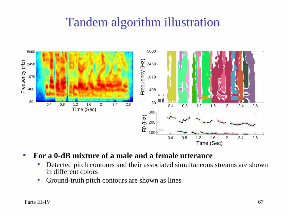
• For a 0-dB mixture of a male and a female utterance • Detected pitch contours and their associated simultaneous streams are shown

in different colors

• Ground-truth pitch contours are shown as lines

Fre

quency (

Hz)

Time (Sec)0.4 0.8 1.2 1.6 2 2.4 2.8

80

408

1079

2458

5000

Fre

quency (

Hz)

0.4 0.8 1.2 1.6 2 2.4 2.880

408

1079

2458

5000

0.4 0.8 1.2 1.6 2 2.4 2.8

100

200

300

F0 (

Hz)

Time (Sec)

Parts III-IV 67

Pitch determination evaluation

-5 0 5 10 150

20

40

60

80

100

Pe

rce

nta

ge

of d

ete

ctio

n

SNR (dB)

Iterative algorithmBoersma and Weenink '04Wu et al. '03

Tandem algorithm

For mixtures of speech with both speech and nonspeech intrusions

Parts III-IV 68

Voiced speech segregation evaluation

For a corpus of voiced speech mixed with 10 different intrusions (Cooke’93)

Mixture

Segregated

Parts III-IV 69

Unvoiced speech segregation

• Unvoiced speech constitutes about 20-25% of all speech sounds

• It carries crucial information for speech intelligibility

• Unvoiced speech is more difficult to segregate than voiced speech

• Voiced speech is highly structured, whereas unvoiced speech lacks harmonicity and is often noise-like

• Unvoiced speech is usually much weaker than voiced speech and therefore more susceptible to interference

• K. Hu and Wang (2011) recently performed unvoiced speech segregation from nonspeech interference using periodic signal removal, spectral subtraction, and segment classification

Parts III-IV 70

Periodic signal removal

• With voiced speech segregated, periodic portions of interference are removed by cross-channel correlation

• Advantages of periodic signal removal

• Periodic signal removal excludes T-F units dominated by voiced speech and periodic interference

• The removal of periodic components of interference makes the remaining interference more stationary

Fre

quency (

Hz)

Parts III-IV 71

Spectral subtraction

• Noise is estimated by averaging energy of masked aperiodic T-F units in voiced intervals (stationarity assumption)

• Spectral subtraction

• is the local SNR at channel c and frame m

• A T-F unit is labeled as unvoiced speech dominant if and only if

• Segments are formed by merging neighboring T-F units

2

2 2ˆ ˆ( , ) | ( , ) | | ( , ) | | ( , ) |c m X c m N c m N c m

( , ) 0c m

( , )c m

Parts III-IV 72

Illustration of spectral subtraction

Removed voiced speech & periodic signals

Candidate unvoiced segments

Mixture

Parts III-IV 73

Unvoiced speech grouping

• We analyze energy distribution of unvoiced speech and

interference segments with respect to their frequency

bounds (shown below)

• Based on this analysis, we group segments with a lower

frequency bound above 2 kHz or an upper bound above

6 kHz as unvoiced speech (i.e. simple thresholding)

Open bar: speech; filled bar: noise Parts III-IV 74

Evaluation and comparison

• Large SNR improvements are achieved by simple thresholding

• Substantially outperform representative speech enhancement algorithms: spectral subtraction (SS) and a priori SNR based Wiener filtering (Wiener-as)

Parts III-IV 75

Examples of unvoiced speech segregation

Input SNR is 0 dB

Noise type Unprocessed

mixture

Voiced speech

segregation only

Voiced speech + unvoiced

speech segregation

Fan noise

Rock music

Parts III-IV 76

Other development: Music separation

• Binary masking can be applied to musical sound separation

• A unique problem is overlapping harmonics

• Western music favors the twelve-tone equal temperament scale, with musical intervals commonly having pitch relationship very close to simple integer ratio

• Li & Wang (2009) considered 2-source separation using pitch based labeling

• Temporal context is used to deal with overlapping harmonics

• Based on the observation that the signal from the same source has similar spectral shapes

• For an overlapped harmonic, labeling is based on the estimated amplitudes of overlapped harmonics from non-overlapped harmonics

Parts III-IV 77

Music separation example

0.5 1 1.5 2 2.5 3 3.5 4 4.5 5-1

0

1

(a)

0.5 1 1.5 2 2.5 3 3.5 4 4.5 5-0.4-0.2

00.20.4

(b)

0.5 1 1.5 2 2.5 3 3.5 4 4.5 5

-0.4-0.2

00.20.4

(c)

0.5 1 1.5 2 2.5 3 3.5 4 4.5 5

-0.5

0

0.5

(d)

0.5 1 1.5 2 2.5 3 3.5 4 4.5 5

-0.5

0

0.5

(e)

Time (s)

Parts III-IV 78

Traditional CASA: Interim summary

• Main progress occurs in voiced speech segregation

• Accomplished with minimal assumptions

• Reliable pitch tracking is important for CASA

• Recent work starts to address unvoiced speech

segregation

Parts III-IV 79

Segregation as classification

Monaural speech segregation

A GMM based algorithm to improve intelligibility

An SVM based algorithm for speech separation

A DNN based large scale training algorithm

Binaural speech segregation

Parts III-IV 80

The approach

Speech intelligibility results reported earlier support the IBM as an appropriate goal of CASA in general, and speech segregation in particular

Hence the speech segregation problem can be formulated as a binary classification problem

Parts III-IV 81

GMM-based classification

Instead of treating voiced speech and unvoiced speech

separately, a simpler approach is to perform

classification on noisy speech regardless of voicing

A classification model by Kim, Lu, Hu, and Loizou

(2009) deals with speech segregation in a speaker and

masker dependent way:

AM spectrum (AMS) features are used

Classification is based on Gaussian mixture models (GMM)

Speech intelligibility evaluation is performed with normal-hearing

listeners

Parts III-IV 82

Diagram of Kim et al.’s model

Parts III-IV 83

Feature extraction and GMM

Peripheral analysis is done by a 25-channel mel-

frequency filter bank

A 15-dimensational AMS feature vector is extracted

within each T-F unit

This vector is then concatenated with the delta vectors over time and

frequency to form a 45-dimensional feature vector for each unit

One GMM (λ1) models target-dominant T-F units and

another GMM models (λ0) noise-dominant units

Each GMM has 256 Gaussian components

Parts III-IV 84

Training and classification

To improve efficiency, each GMM is subdivided into two

models during training: one for relatively high local

SNRs and one for relatively low SNRs

With the 4 trained GMMs, segregation comes down to

Bayesian classification with prior probabilities of P(λ0)

and P(λ1) estimated from the training data

The training and test data are mixtures of IEEE

sentences and 3 masking noises: babble, factory, and

speech-shaped noise

Separate GMMs are trained for each speaker (a male and a female)

and each masker

Parts III-IV 85

A separation example

Target utterance

-5 dB mixture with

babble

Estimated mask

Masked mixture

Parts III-IV 86

Intelligibility results and demo

Clean: 0-dB mixture with babble: Segregated:

UN: unprocessed

IdBM: ideal binary mask

sGMM: trained on a single noise

mGMM: trained on multiple noises

Parts III-IV 87

Discussion

GMM classifier achieves a hit rate (active units correctly

classified) higher than 80% for most cases while keeps

the false-alarm (FA) rate relatively low

As expected, mGMM results are worse than sGMM

HIT – FA well correlates with intelligibility

The first monaural separation algorithm to achieve

significant speech intelligibility improvements

Main limitation is speaker and masker dependency

Parts III-IV 88

SVM-based classification (Han & Wang’12)

• Feature extraction

• Pitch: autocorrelation values at detected pitch lags

• AMS

• Unit labeling using support vector machine (SVM)

• Segmentation

• Voiced frames: Cross-channel

• Unvoiced frames: Onset/offset analysis

Parts III-IV 89

Support vector machine

• Train an SVM for each channel (64 channels)

• Gaussian kernels are used

• Issue:

• Classification accuracy or HIT-FA (false alarm), which is highly

correlated to speech intelligibility (Kim et al.’09)?

• Re-thresholding technique

• Instead of 0, we choose a new threshold to maximize HIT-FA in each

channel c

• θc is chosen from a small validation set

Parts III-IV 90

Re-thresholding Segmentation

IBM

Re-thresholding

SVM labeling

Segmentation

Estimated IBM

Parts III-IV 91

Classification results

• Compared to Kim et al.’09 system (AMS+GMM), this SVM classifier

achieves higher HIT-FA rates, particularly for unseen noises

Parts III-IV 92

Demo

• Female Speech + Factory Noise (0 dB)

• Noisy speech

• Proposed

• IBM

Parts III-IV 93

Generalization via expanded training

• Generalization is an extremely important issue for supervised learning

• A straightforward approach to generalization is to train on a large variety of acoustic conditions

• For kernel machines, however, large-scale training is almost intractable due to computational complexity

• We propose to learn more linearly separable and discriminative features from raw data via deep neural networks (DNNs) and then train linear SVM for classification (Wang & Wang’13)

• DNNs can be viewed as hierarchical feature detectors

Parts III-IV 94

Deep neural networks

• Why deep?

• Automatically learn more abstract features as the number of layers

increases

• More abstract features tend to be more invariant to superficial

variations

• Superior performance in practice if properly trained (e.g., convolutional

neural networks)

• However, deep structure is hard to train from random

initializations

• Vanishing gradients: Error derivatives tend to become very small in

lower layers, causing overfitting in upper layers

• Hinton et al. (2006) suggest to unsupervisedly pretrain the

network using restricted Boltzmann machines (RBMs)

Parts III-IV 95

DNN training

• Unsupervised, layer-by-layer RBM pretraining

• Train the first RBM using unlabeled data

• Fix the first layer weights. Use the resulting hidden activations as new

features to train the second RBM

• Continue until all layers are thus trained

• Supervised fine-tuning

• The weights from RBM pretraining provide the network initialization

• Use standard backpropagation to fine tune all the weights to a particular task

Parts III-IV 96

DNN as subband classifier

• DNN is used for feature learning from raw acoustic features

• Train DNNs in the standard way. After training, take the last hidden layer

activations as learned features

• Train SVMs using the combination of raw and learned features

• Linear SVM seems adequate

• The weights from the last hidden layer to the output layer essentially define a

linear classifier

• Therefore the learned features are amenable to linear classification

Parts III-IV 97

DNN as subband classifier

Parts III-IV 98

Large training with DNN

• Training on 200 randomly chosen IEEE utterances from

both male and female speakers, mixed with 100

environmental noises (Hu, 2006) at 0 dB (~17 hours long)

• Six million fully dense training samples in each channel,

with 64 channels in total

• Evaluated on 20 unseen speakers mixed with 20 unseen

noises at 0 dB

Parts III-IV 99

DNN-based separation results

• Comparisons with a representative speech enhancement algorithm (Hendriks et

al.’10)

• Using clean speech as ground truth, on average about 3 dB SNR improvements

• Using IBM separated speech as ground truth, on average about 5 dB SNR

improvements

Parts III-IV 100

Sound demos

Speech (carrier: "You will say ...")

mixed with speech-shaped noise at -5 dB

Mixture Separated

Mixture Separated

Speech mixed with unseen, daily noises

Mixture Separated

Mixture Separated

Cocktail party noise (5 dB)

Destroyer noise (0 dB)

Parts III-IV 101

Binaural segregation

• The model by Roman et al. (2003) is probably the first to

address sound separation as a binary classification

problem

• The IBM provides the training labels for supervised

learning

• Segregation amounts to IBM estimation

Parts III-IV 102

Model architecture

Binaural

Cue

Extraction

Pattern

Analysis

Azimuth Localization

Target

Noise

Auditory

Filterbanks

L

R

Resynthesis

R

L

Parts III-IV 103

Azimuth localization

• Cross-correlogram for ITD detection

• Frequency-dependent nonlinear transformation from the time-delay axis to the azimuth axis

• Locations are identified as peaks in the skeleton cross-correlogram

Parts III-IV 104

Binaural cue extraction

• Interaural time difference (ITD)

• Cross-correlation mechanism

• To resolve the multiple-peak problem at high frequencies, ITD is

estimated as the peak in the cross-correlation pattern within a period

centering at ITDtarget

• Interaural intensity difference (IID or ILD): Ratio of

right-ear energy to left-ear energy

2

10 2

( )

IID 10log( )

ij

tij

ij

t

r t

l t

Parts III-IV 105

IBM estimation

• For narrowband stimuli, systematic changes of extracted

ITD and IID values occur as the relative strength of the

original signals changes. This interaction produces

characteristic clustering in the joint ITD-IID space

• The core of the model lies in deriving the statistical

relationship between the relative strength and the

binaural cues

Parts III-IV 106

3-Source Configuration Example

- Data histograms for one channel (center frequency: 1.5 kHz) from

speech sources with target at 0o and two intrusions at -30o and 30o (R:

relative strength)

- Clustering in the joint ITD-IID space

Parts III-IV 107

Binary classification

• Independent supervised learning for different spatial

configurations and different frequency bands in the joint

ITD-IID feature space

• Define:

• Decision rule (MAP):

• Nonparametric method for the estimation of probability

densities : Kernel Density Estimation

• Utterances from the TIMIT corpus are used for training

1 1

2 2

~ ( | ): target dominates ( 0.5)

~ ( | ) : interference dominates ( 0.5)

ij

ij

H p x H R

H p x H R

1 1 2 21, if ( ) ( | ) ( ) ( | )( )

0, else

p H p x H p H p x HM x

)|( iHxp

Parts III-IV 108

Example (Target: 0o, Noise: 30o)

Target Noise Mixture Ideal binary mask Result

Parts III-IV 109

Sound demo

Target

Noise Mixture Segregated target

‘Cocktail Party’

Siren

Female Speech

Noise1 Mixture Segregated target

‘Cocktail Party’

Female Speech

3 sound sources (Target: 0º, Noise1: -30º, Noise2: 30º)

Target

Noise2

2 sound sources (Target: 0º, Noise: 30º)

Parts III-IV 110

Speech intelligibility evaluation

• The Bamford-Kowal-Bench sentence database is used that contains short semantically predictable sentences as target

Mixture Segregated

Two-source (0º, 5º) condition

Interference: babble noise

Three-source (0º, 30º, -30º) condition

Interference: male utterance & female utterance

Parts III-IV 111

Discussion

• The estimation of the ideal binary mask is based on

pattern classification in the joint ITD-IID feature space

• Training is configuration-specific and frequency-specific

• Estimated masks are very similar to ideal ones

• High-quality estimation of the ideal binary mask translates to high

ASR and speech intelligibility scores

• Binaural segregation employs spatial cues, whereas

monaural segregation exploits intrinsic sound

characteristics

• A main challenge in binaural segregation is room

reverberation

• See for example, Roman et al. (2006)

Parts III-IV 112

Classification-based CASA: Interim summary

• Formulation of the segregation problem as binary

classification enables the use of supervised learning

• Studies adopting this classification approach achieve

very promising results

• Particularly for improving speech intelligibility in noise, a long-

standing challenge

Parts III-IV 113

Summary of Part IV

• The primary feature of CASA is that it is perceptually-

motivated

• Emphasis on perceptual characteristics

• Emphasis on sound properties

• In other words, it is content-based analysis

• Advances in traditional and classification-based

methods have made CASA a strong approach to real-

world sound separation

Parts III-IV 114