1

Computational Chemistry and Quantum Tunneling Key Words quantum chemistry, Hartree-Fock theory, density functional theory, variational principle, quantum tunneling, transition state Object

It is expected that students can predict the chemical trends of the inversion of amines and phosphines through calculations, and understand the theoretical backgrounds of computational chemistry and the concept of quantum tunneling.

Introduction

Electron structure theory such as Hartree-Fock and density functional theory (DFT) have made it possible to calculate a variety of properties of molecules. They are also very useful to search the reaction pathway for a given chemical reaction which consists of the free energies of reactants, transition states, and products. Thanks to the rapid development of computer and software for computational chemistry, nowadays people in not only theoretical but also experimental chemistry laboratories use computational chemistry to investigate various molecular properties encompassing geometric structures, spectroscopic information, reaction pathways, etc, and compare them with experimental observations. One of the great advantages of accurate computational chemistry is that it would be capable of predicting molecular properties without experiments, leading to the acceleration of chemical research with inexpensive, rapid manner.

In this experiment, reaction profiles of pyramidal inversion which involves quantum tunneling of a particle trapped in a finite potential are investigated using a modern approach of computational chemistry. Background Information Theory 1. Hartree-Fock(HF) approximation1,2

(McQuarrie Physical Chemistry textbook chapter 9) The total Hamiltonian of a molecule can be written as

n e ne ee nnH T T V V V= + + + + (1)

If we apply the Born-Oppenheimer approximation, the nuclear kinetic energy part Tn can be ignored. The next three terms are electronic Hamiltonian, where Te is the kinetic energy of electrons, Vne is the attraction term between nuclei and electrons, and Vee is electron-electron repulsion term, respectively. Vnn is the nucleus-nucleus repulsion term. Then Eq. (1) can be

2

written as

21 1 (2)2

e ne ee nn

A A Bi

i A i ij ABiA ij AB

H T V V VZ Z Zr r R

= + + +

= − − + +∑ ∑∑ ∑ ∑∇

where the indices ,i j indicate the electrons and A for nuclei, respectively. AZ is the

charge of the nucleus A . The energy of the molecule can be evaluated,

| | (3)E H=< Φ Φ >

The Hartree-Fock approximation introduces a Slater determinant for wavefunction which is antisymmetric:

1 1 1 2 1

2 1 2 2 2

1 2

( ) ( ) ( )( ) ( ) ( )

(4)

( ) ( ) ( )

N

N

N N N N

χ χ χχ χ χ

χ χ χ

Φ =

x x xx x x

x x x

where ( ) ( ) ( )i j i j i jwχ φ α=x r are one-electron spin orbitals and ( , )j j jw=x r indicates the

spatial and spin coordinates. The spin coordinate can be either α or β for up or down spin, respectively. The electronic Hamiltonian can be rewritten as the sum of one-electron part ih , i.e. core Hamiltonian and two-electron repulsion part 1

ijr − ,

1

1 1

ˆ (5)N N

elec e ne ee i iji i j i

H T V V h r −

= = >

= + + = +∑ ∑∑

where 21ˆ2

Ai i

iA

Zhr

= − −∇ , which consists of electron kinetic energy and electron-nucleus

attraction operator. The one-electron contribution of total energy is

(1) *1 1 1 1

1 1 1

ˆ ˆ( ) ( ) ( ) [ | | ] (6)N N N

i i i ii ii i i

E d h h i h iσ σ

χ χ= = =

= = =∑∑ ∑∑ ∑∫ x x x x

where σ indicates the spin index and N is the number of electrons. Two-electron contribution is more complicated. It consists of Coulomb and exchange integrals ijJ and ijK :

* 1 *1 2 1 1 12 2 2

* 1 *1 2 1 1 12 2 2

( ) ( ) ( ) ( ) [ | ]

( ) ( ) ( ) ( ) [ | ] (7)

ij i i j j

ij i j j i

J d d r ii jj

K d d r ij ji

χ χ χ χ

χ χ χ χ

−

−

= =

= =

∫∫

x x x x x x

x x x x x x

Then the energy becomes (2)

, 1 1 1 1

1 1 (8)2 2

i j

N N N N

ij iji j i j

E J Kσ σ σ= = = =

= −∑ ∑∑ ∑∑∑

The Coulomb integral is the classical repulsive energy between two charges and the exchange integral is a stabilization energy arisen from the antisymmetric property of the wavefunction.

3

The exchange integral acts only between the electrons of the same spin due to the Pauli exclusion principle. Finally, the Hartree-Fock energy is

1 , 1 1 1 1

1 1 (9)2 2

i j

N N N N N

HF ii ij iji i j i j

E h J Kσ σ σ= = = = =

= + −∑ ∑ ∑∑ ∑∑∑

Now the energy is minimized under orthonormality condition of spin orbitals. Using Lagrange multiplier method,

1 1{ ( )} 0 (10)

N N

HF ij iji j

E i jδ ε δ= =

− − =∑∑

where *

1 2 1 2( ) ( ) (11)i ji j d d x xχ χ= ∫ x x

The Hartree-Fock equation as an one-electron Schrodinger-like equation can be derived by solving Eq. (10). That is,

1 1 1 11

ˆ ˆ ˆ[ ( ) ( )] ( ) ( ) (12)N N

j j i ij jj i j

h J K φ ε φ≠ =

+ − =∑ ∑r r r

where ˆ ˆ,j jJ K are the Coulomb and exchange operator. 3 * 1

1 2 2 12 2 1

3 * 11 2 2 12 2 1

ˆ ( ) ( ) ( ) ( )

ˆ ( ) ( ) ( ) ( ) (13)

{ }{ }

j i j j i

j i j i j

J d r

K d r

φ φ φ φ

φ φ φ φ

−

−

=

=

∫∫

r r r r r

r r r r r

The parenthesis on the left-hand side of eq. (12) is called the Fock operator, F . 2. Density functional theory (DFT)2,3 For the N electron system, the wave function has 3N spatial coordinates. However, regardless of the number of electrons, the electron density has only 3 spatial coordinates. Therefore the electron density rather than the wavefunction is more efficient to describe the electronic structure of molecules. DFT states that the ground energy of a system can be determined solely from the electron density by virtue of the Hohenberg-Kohn theorem: Theorem 1 : There is one-to-one relationship between the ground state electron density ρ and the external potential extv . Theorem 2 : For a trial density ( )ρ r , such that ( ) 0ρ ≥r and 3 ( )d r Nρ =∫ r ,

0 [ ]. (14)vE E ρ≤ where [ ]vE ρ is the variational energy functional.

3 3[ ] [ ] [ ] ( ) ( ) [ ] ( ) ( ) (15)v ee ext extE T U d r v F d r vρ ρ ρ ρ ρ ρ= + + = +∫ ∫r r r r

[ ]T ρ is the kinetic energy functional and [ ]eeU ρ is the electron-electron repulsion energy

functional.

4

If the functional form of [ ]F ρ , which is universal regardless of systems represented by extv ,

is known, in principle, one can exactly calculate the energy of the molecule, since the external potential is readily known. Unfortunately, however, the exact functional form is unknown. Kohn and Sham proposed that a non-interacting system, which produces the same electron density with that of the interacting system, gives the same energy, as the first Hohenberg-Kohn theorem tells. The kinetic energy and the electron density of the non-interacting system can be expressed in terms of one-electron orbitals like Hartree-Fock approximation (Eq. (4)),

22

1( ) | | ( ) (16)

2

N

s i i ii

T fm

φ φ=

= − < ∇ >∑ r r

*

1( ) ( ) ( ) (17)

N

i i ii

fρ φ φ=

=∑r r r

where if is the occupation number. Using non-interacting kinetic energy, the universal functional [ ]F ρ can be rewritten as

[ ] [ ] [ ] [ ] [ ] [ ] (18)ee s xcF T U T J Eρ ρ ρ ρ ρ ρ= + = + + where [ ]J ρ is the Coulomb term,

'3 3 '

'

1 ( ) ( )[ ] . (19)2 | |

J d rd r ρ ρρ =−∫

r rr r

and [ ]xcE ρ is the exchange-correlation energy which includes the kinetic correlation(i.e. [ ] [ ]sT Tρ ρ− ). Finally, the Kohn-Sham functional becomes

'3 3 3 '

'

1 ( ) ( )[ ] [ ] ( ) ( ) [ ] (20)2 | |KS s ext xcE T d r v d rd r Eρ ρρ ρ ρ ρ= + + +

−∫ ∫r rr rr r

Like we have done in the Hartree-Fock approximation, Eq. (10), this energy is minimized using the Lagrange multiplier method. Then we can obtain the one-electron Schrodinger-like Kohn-Sham equation which is

'2 3 '

'

1 ( ) ( ) ( ) ( ) ( ) (21)2 | |

( )xc ext m m md r v vρ φ ε φ− ∇ + + + =−∫r r r r r

r r

where ( )xcv r is the exchange-correlation potential, [ ]( ) (22)xc

xcEv δ ρδρ

=r

There are many known density functionals which have different functional forms of [ ]xcE ρ .

Though both DFT and HF have similar features, in particular, one-electron representation of many body systems, DFT is mostly better than HF because DFT does have electron correlation term, whereas HF completely ignores it. 3. Electron density and correlation2,3 The one-body density matrix is

*1 2 2 2( , ') ( , , , ) ( , , , ) (23)N N NN d dρ ψ ψ= ∫ 'r r r r r r r r r r

5

The diagonal elements of matrix is the electron density, 2

1 2 2( , ) ( ) | ( , , , ) | (24)N NN d dρ ρ ψ= = ∫r r r r r r r r

The total number of electron is, ( ) (25)N d ρ= ∫ r r

The two-body density matrix can also be defined, *

2 1 2 1 2 3 1 2 1 2( 1)( , ) ( , , , ) ( , , , ) (26)

2 N N NN N d dρ ψ ψ−

= ∫' ' ' 'r r r r r r r r r r r r

and the diagonal elements are 2

2 2 3( 1)( , ) ( , ) | ( , , , ) | (27)

2 N NN N d dρ ρ ψ−

= = ∫' ' ' 'rr r r r r r r r r r

2 ( , )ρ 'r r is the probability of finding electrons at r and 'r .

Now the concept of correlation is understood by using these definitions of electron density and density matrix. If there is no interaction between electrons (uncorrelated), the elements of two-body density matrix are simply the product of electron densities,

21( , ) ( ) ( ) (28)2

ρ ρ ρ=' 'r r r r

If there exists correlation,

21( , ) ( ) ( )[1 ( , )] (29)2

gρ ρ ρ= +' ' 'r r r r r r

where ( , )g 'r r is the pair correlation function. It is zero if two electrons are separated at an

infinite distance and different from zero when r is close to 'r . Hartree-Fock contains no correlation effects, whereas in case of DFT, the correlation term can be included in the functional [ ]xcE ρ .

4. Self-interaction2 Recall the Coulomb term in DFT, Eq. (19),

'3 3 '

'

1 ( ) ( )[ ] . (30)2 | |

J d rd r ρ ρρ =−∫

r rr r

Applying this term to one-electron system whose wave function is ( )φ r , 2[| ( ) | ] 0. (31)J φ ≠r

Thus there exists the repulsion energy with itself, i.e. the self-interaction energy. If one can find the exact form of [ ]xcE ρ , the self-interaction energy can be completely

cancelled. However, so far, it is not possible. When it comes to Hartree-Fock, there is no self-interaction, because there exists the cancellation of the self-interaction energy, ii iiJ K= .

6

5. Basis sets1 (McQuarrie Physical Chemistry textbook chapter 11) A basis set is a set of functions used to construct trial molecular orbitals according to the variational principle, which are expanded as a linear combination of certain primitive functions such as Gaussian functions.

1(33)

K

i icµ µµ

ψ φ=

=∑

Gaussian type basis sets rather than Slater type are often used in computations for the sake of convenience. For instance, ‘X-YZG*’ indicates that core orbitals are formulated by X Gaussians and valence orbitals are formulated by two atomic basis functions, one consists of Y Gaussian primitives and the other, Z primitives, respectively. ‘*’ at the end means that polarization functions has been added. For example, 6-31G* basis sets for a carbon atom:

- Core : 1s orbital : 1-zeta function represented by 6 Gaussian functions - Valence : 2s and 2p orbitals : 2-zeta functions represented by 3 and 1 Gaussian

functions, respectively. - Polarization : 3d orbitals have been added.

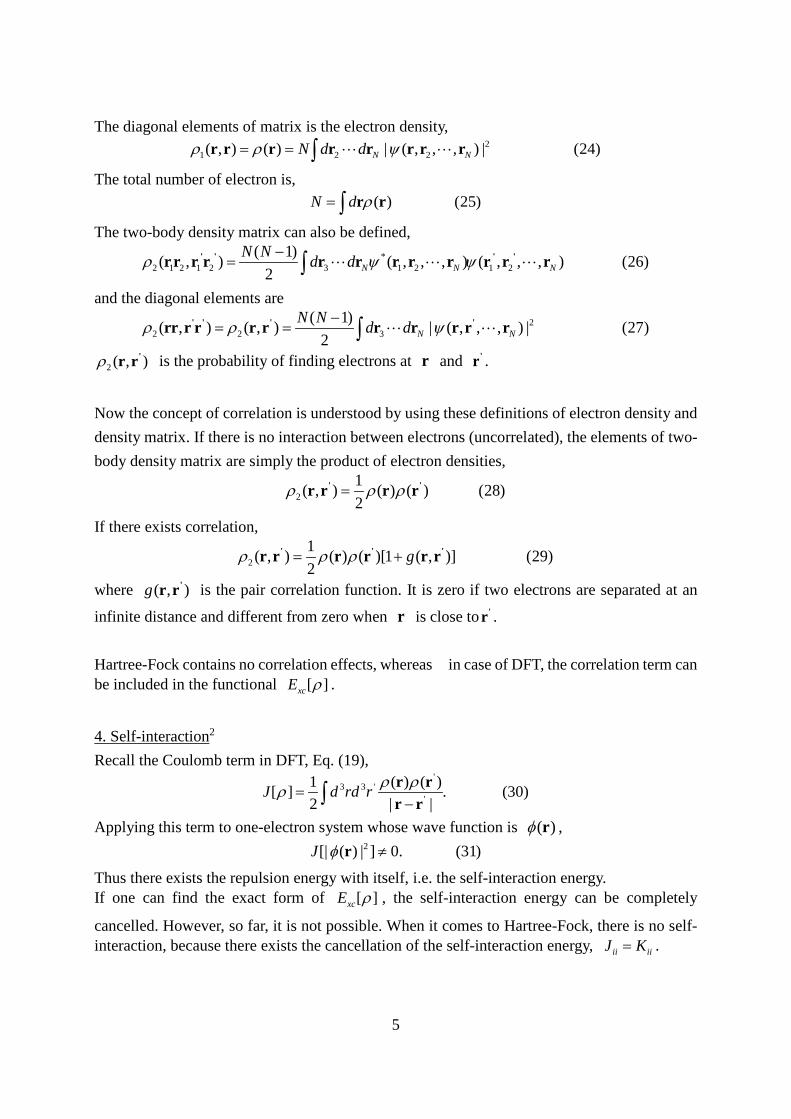
6. Quantum tunneling5 Let us consider an one-dimensional system whose potential is given as

1

0( ) (34)

if x L or L xV x

V if L x L≤ − ≤

= − < <

It has barrier at L x L− < < whose height is 1( 0)V > . Classically, if particle’s total energy is less than 1V , it cannot pass through the barrier. However, a quantum particle has a probability to

pass through the barrier. This phenomenon is called the quantum tunneling.

7

Inversion of amines or phosphines is a good example of quantum tunneling in nature. Further examples of quantum tunneling in various chemical reactions are also reported.9 Equipment No special equipment for this experiment.

Figure 1. Quantum tunneling.

8

Pre-Laboratory Questions

1. What are pros and cons of DFT in terms of self-interaction and electron correlation compared to the HF method? 2. If we use 3-21G* basis set for calculation of the ammonia (NH3) molecule, how many basis functions are used for calculations? 3. Explain the quantum tunneling phenomenon in terms of the Heisenberg uncertainty principle. 4. How is the inversion of amines and phosphines related to the quantum tunneling? Materials Reagents No reagents. Apparatus Laptop provided, and the Avogadro program (It is free and you can download it easily from websites. You may practice this program before lab.7) Safety and Hazards No hazards.

9

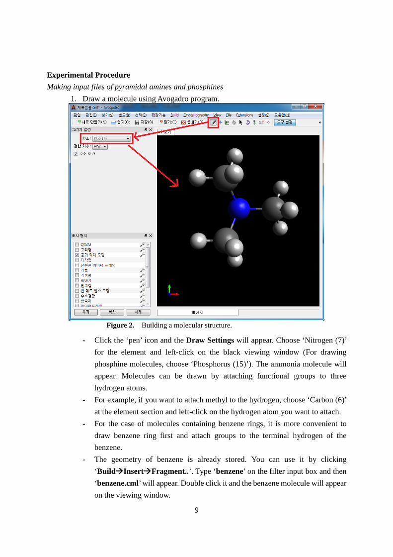
Experimental Procedure Making input files of pyramidal amines and phosphines

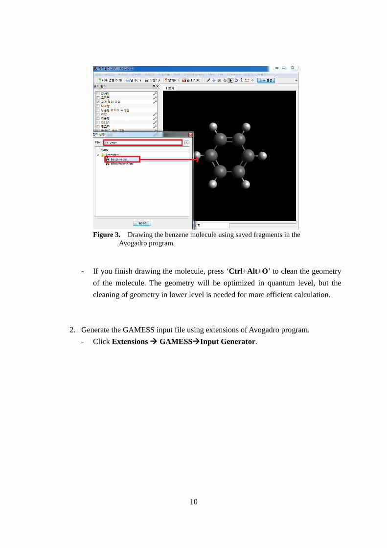
1. Draw a molecule using Avogadro program.

- Click the ‘pen’ icon and the Draw Settings will appear. Choose ‘Nitrogen (7)’ for the element and left-click on the black viewing window (For drawing phosphine molecules, choose ‘Phosphorus (15)’). The ammonia molecule will appear. Molecules can be drawn by attaching functional groups to three hydrogen atoms.

- For example, if you want to attach methyl to the hydrogen, choose ‘Carbon (6)’ at the element section and left-click on the hydrogen atom you want to attach.

- For the case of molecules containing benzene rings, it is more convenient to draw benzene ring first and attach groups to the terminal hydrogen of the benzene.

- The geometry of benzene is already stored. You can use it by clicking ‘BuildInsertFragment..’. Type ‘benzene’ on the filter input box and then ‘benzene.cml’ will appear. Double click it and the benzene molecule will appear on the viewing window.

Figure 2. Building a molecular structure.

10

- If you finish drawing the molecule, press ‘Ctrl+Alt+O’ to clean the geometry of the molecule. The geometry will be optimized in quantum level, but the cleaning of geometry in lower level is needed for more efficient calculation.

2. Generate the GAMESS input file using extensions of Avogadro program. - Click Extensions GAMESSInput Generator.

Figure 3. Drawing the benzene molecule using saved fragments in the Avogadro program.

11

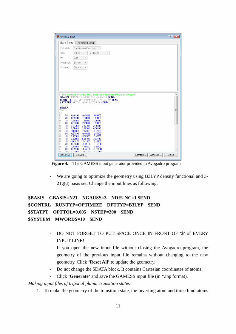
- We are going to optimize the geometry using B3LYP density functional and 3-

21g(d) basis set. Change the input lines as following: $BASIS GBASIS=N21 NGAUSS=3 NDFUNC=1 $END $CONTRL RUNTYP=OPTIMIZE DFTTYP=B3LYP $END $STATPT OPTTOL=0.005 NSTEP=200 $END $SYSTEM MWORDS=10 $END

- DO NOT FORGET TO PUT SPACE ONCE IN FRONT OF ‘$’ of EVERY INPUT LINE!

- If you open the new input file without closing the Avogadro program, the geometry of the previous input file remains without changing to the new geometry. Click ‘Reset All’ to update the geometry.

- Do not change the $DATA block. It contains Cartesian coordinates of atoms. - Click ‘Generate’ and save the GAMESS input file (in *.inp format).

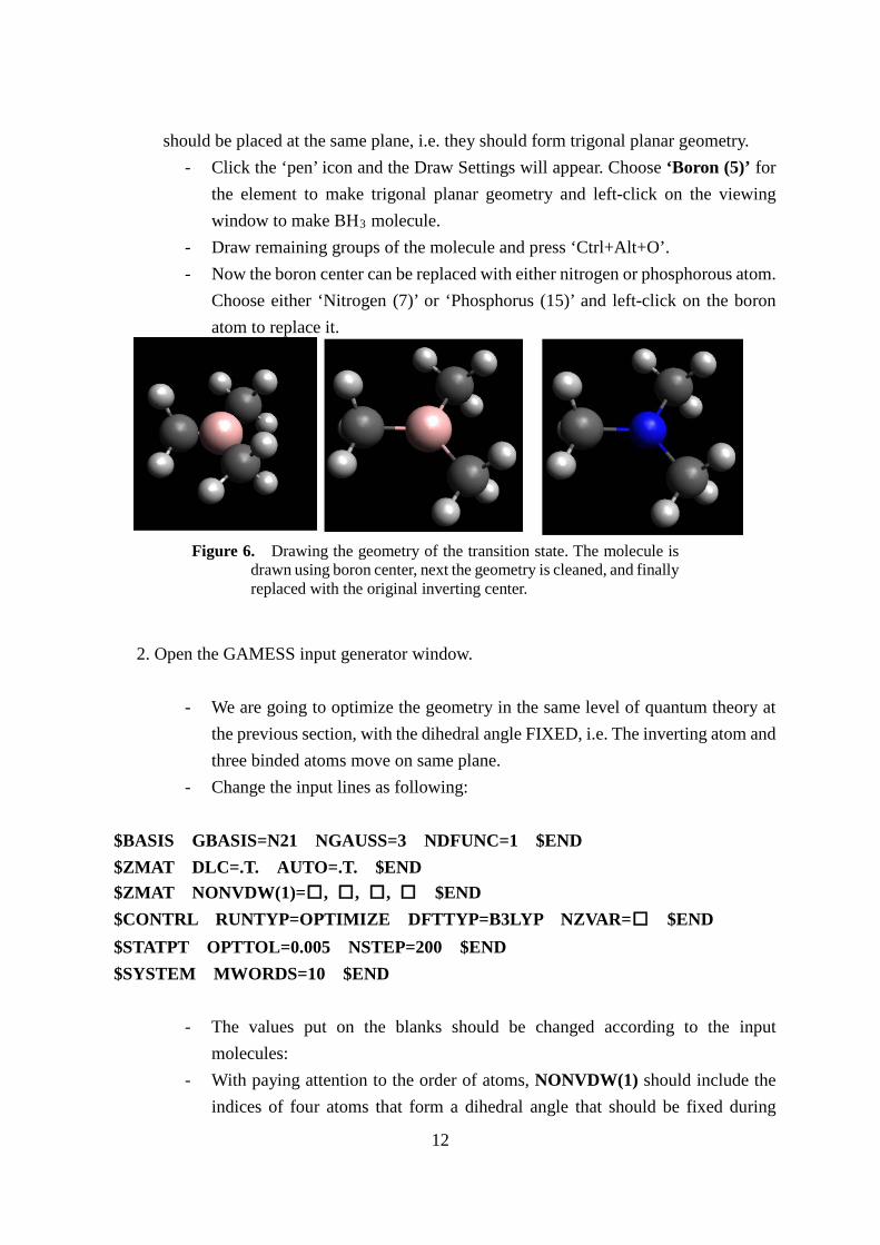
Making input files of trigonal planar transition states 1. To make the geometry of the transition state, the inverting atom and three bind atoms

Figure 4. The GAMESS input generator provided in Avogadro program.

12

should be placed at the same plane, i.e. they should form trigonal planar geometry. - Click the ‘pen’ icon and the Draw Settings will appear. Choose ‘Boron (5)’ for

the element to make trigonal planar geometry and left-click on the viewing window to make BH3 molecule.

- Draw remaining groups of the molecule and press ‘Ctrl+Alt+O’. - Now the boron center can be replaced with either nitrogen or phosphorous atom.

Choose either ‘Nitrogen (7)’ or ‘Phosphorus (15)’ and left-click on the boron atom to replace it.

2. Open the GAMESS input generator window.

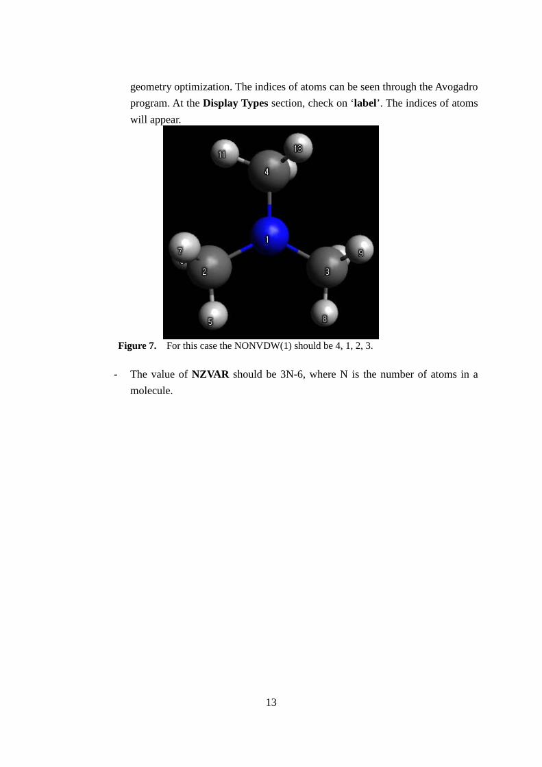
- We are going to optimize the geometry in the same level of quantum theory at the previous section, with the dihedral angle FIXED, i.e. The inverting atom and three binded atoms move on same plane.

- Change the input lines as following: $BASIS GBASIS=N21 NGAUSS=3 NDFUNC=1 $END $ZMAT DLC=.T. AUTO=.T. $END

$ZMAT NONVDW(1)=□, □, □, □ $END $CONTRL RUNTYP=OPTIMIZE DFTTYP=B3LYP NZVAR=□ $END $STATPT OPTTOL=0.005 NSTEP=200 $END $SYSTEM MWORDS=10 $END

- The values put on the blanks should be changed according to the input

molecules: - With paying attention to the order of atoms, NONVDW(1) should include the

indices of four atoms that form a dihedral angle that should be fixed during

Figure 6. Drawing the geometry of the transition state. The molecule is drawn using boron center, next the geometry is cleaned, and finally replaced with the original inverting center.

13

geometry optimization. The indices of atoms can be seen through the Avogadro program. At the Display Types section, check on ‘label’. The indices of atoms will appear.

- The value of NZVAR should be 3N-6, where N is the number of atoms in a

molecule.

Figure 7. For this case the NONVDW(1) should be 4, 1, 2, 3.

14

Calculation and analysis of the output file 1. Put the GAMESS input file into the Edison chem site and call the GAMESS program. Wait until the calculation is terminated.

- Go to the Edison_chem website http://chem.edison.re.kr/ and login (ID and password will be announced by TA).

- Click ‘Simulation’ and choose the software ‘The General Atomic and Molecular Electronic Structure System (GAMESS)’. Click ‘Next step’.

- Briefly write the name and description of the simulation at the instance

information part, go to the Input Port part at the bottom.

Figure 9. Write the simulation name and description

Figure 8. At the simulation section, find the GAMESS program and select it, and go on to the next step.

15

- Select Insert Data and insert input file made by Avogadro program

- Click ‘Job submission status’ and the task will appear at the list. Click ‘Submit

job’.

Figure 9. Putting GAMESS input file into the EDISON system.

Figure 10. Submit job to the GAMESS program.

16

- Click ‘Monitoring’ and check simulation status. - There are four states : Purple color – queue, skyblue – running, green – success,

and red – fail. Wait until the green button appears. If the error occurs, check the input file and fix errors.

- You can check running progress progress, download the ouput files and see

visualizations such as electron density and molecular orbitals.

Figure 11. The monitoring window. The running status can be checked.

17

2. Open the log file using WordPad. Find the line containing ‘TOTAL ENERGY = ’. It appears twice, and you should read the energy value of the last one. That is the calculated energy value of the optimized geometry in Hartree unit.

3. Find the word ‘EIGENVECTORS’ in your log file. At that section, energies of each orbital are written. Find HOMOs and write down the energy value if you need.

Figure 12. Visualization through Jmol program.

18

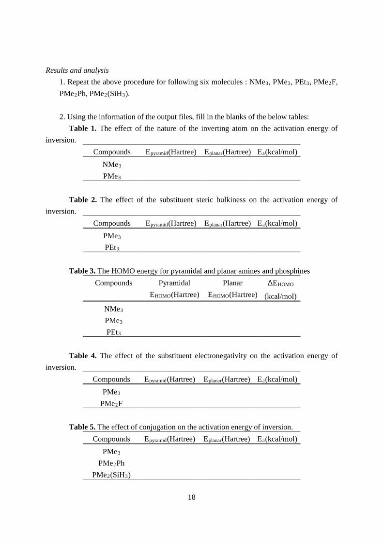
Results and analysis

1. Repeat the above procedure for following six molecules : NMe3, PMe3, PEt3, PMe2F, PMe2Ph, PMe2(SiH3).

2. Using the information of the output files, fill in the blanks of the below tables:

Table 1. The effect of the nature of the inverting atom on the activation energy of inversion.

Compounds Epyramid(Hartree) Eplanar(Hartree) Ea(kcal/mol) NMe3 PMe3

Table 2. The effect of the substituent steric bulkiness on the activation energy of

inversion. Compounds Epyramid(Hartree) Eplanar(Hartree) Ea(kcal/mol)

PMe3 PEt3

Table 3. The HOMO energy for pyramidal and planar amines and phosphines

Compounds Pyramidal EHOMO(Hartree)

Planar EHOMO(Hartree)

ΔEHOMO

(kcal/mol) NMe3 PMe3 PEt3

Table 4. The effect of the substituent electronegativity on the activation energy of

inversion. Compounds Epyramid(Hartree) Eplanar(Hartree) Ea(kcal/mol)

PMe3 PMe2F

Table 5. The effect of conjugation on the activation energy of inversion.

Compounds Epyramid(Hartree) Eplanar(Hartree) Ea(kcal/mol) PMe3

PMe2Ph PMe2(SiH3)

19

20

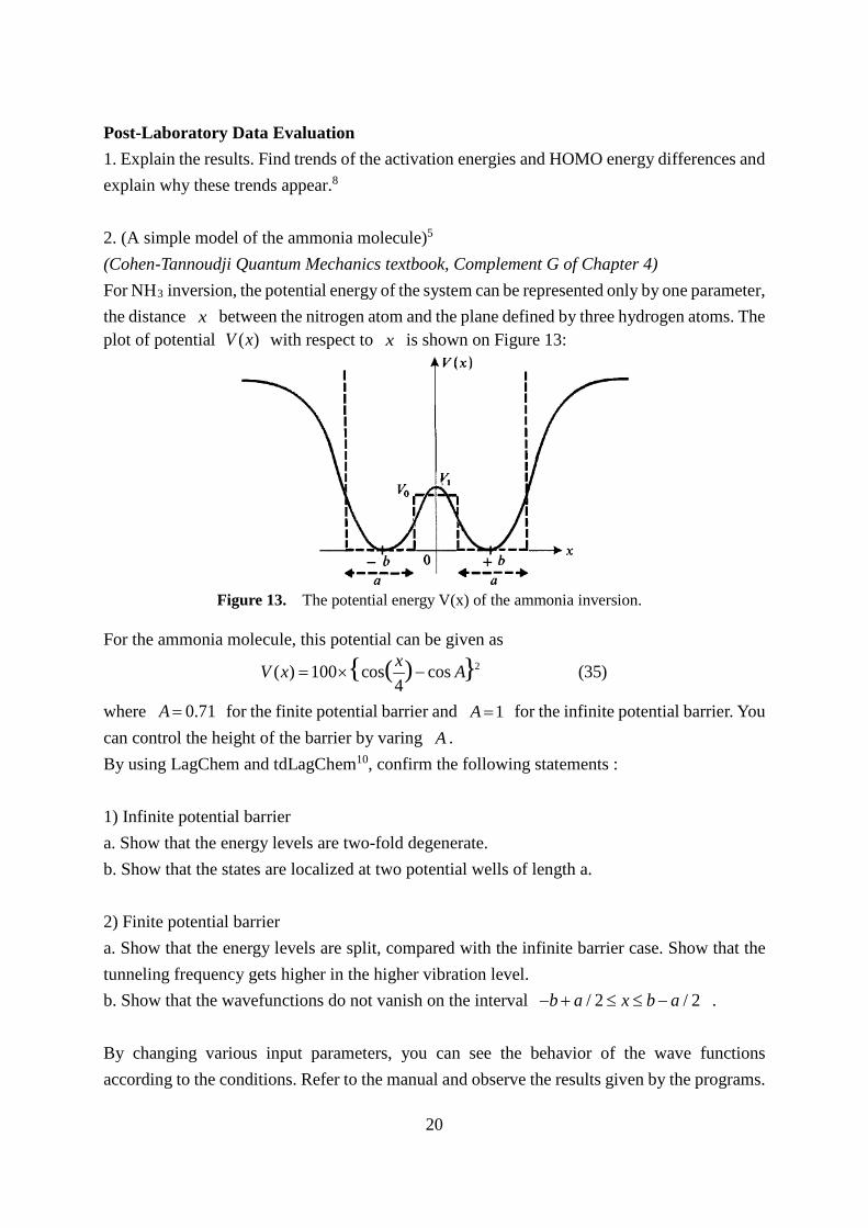
Post-Laboratory Data Evaluation 1. Explain the results. Find trends of the activation energies and HOMO energy differences and explain why these trends appear.8 2. (A simple model of the ammonia molecule)5 (Cohen-Tannoudji Quantum Mechanics textbook, Complement G of Chapter 4) For NH3 inversion, the potential energy of the system can be represented only by one parameter, the distance x between the nitrogen atom and the plane defined by three hydrogen atoms. The plot of potential ( )V x with respect to x is shown on Figure 13:

For the ammonia molecule, this potential can be given as

2( ) 100 cos cos (35)4

( ){ }xV x A= × −

where 0.71A = for the finite potential barrier and 1A = for the infinite potential barrier. You can control the height of the barrier by varing A . By using LagChem and tdLagChem10, confirm the following statements : 1) Infinite potential barrier a. Show that the energy levels are two-fold degenerate. b. Show that the states are localized at two potential wells of length a. 2) Finite potential barrier a. Show that the energy levels are split, compared with the infinite barrier case. Show that the tunneling frequency gets higher in the higher vibration level. b. Show that the wavefunctions do not vanish on the interval / 2 / 2b a x b a− + ≤ ≤ − . By changing various input parameters, you can see the behavior of the wave functions according to the conditions. Refer to the manual and observe the results given by the programs.

Figure 13. The potential energy V(x) of the ammonia inversion.

21

References 1. Attila Szabo and Neil S. Ostlund, Modern Quantum Chemistry: Introduction to Advanced

Electronic Structure Theory, Dover Publications, Inc: New York, 1996. 2. Jorge Kohanoff, Electronic structure calculations for solids and molecules: Theory and

Computational Methods, Cambridge University Press, 2006. 3. Wolfram Koch and Max C. Holthausen, A Chemist's Guide to Density Functional Theory,

2nd ed.; Wiley-VCH, 2001. 4. J. Chem. Phys. 98, 5648 (1993). 5. Claude Cohen-Tannoudji, Bernard Diu, and Franck Laloe, Quantum Mechanics, Wiley-VCH,

2005. vol. 1, pp 67-78, 455-469. 6. GAMESS Manual. http://wild.life.nctu.edu.tw/~jsyu/gamess2k/ 7. Get Avogadro. http://avogadro.openmolecules.net/wiki/Get_Avogadro 8. J. Chem. Educ. 90, 661 (2013). 9. Quantum Tunneling in Chemical Reactions, Diane Carrera. http://www.princeton.edu/chemistry/macmillan/group-meetings/DEC_tunneling.pdf 10. Manual for tdLagChem & LagChem using EDISON. (file uploaded)