computational fluid dynamics, cfd and experimental · pdf filetheory of turbo machinery /...
TRANSCRIPT

Theory of turbo machinery / Turbomaskinernas teori
Beyond Dixon
Computational Fluid Dynamics, CFD and Experimental methods

Det blir åttahundra grader. Du kan lita på mej. du kan lita på mej.
(Ebba Grön)

LTH / Kraftverksteknik / JK
1. Control Volume or large scale analyses2. Differential analyses (NS-equations)3. Experiments and/or dimensional
analyses
Basic approachs (F.M. White)
Background

LTH / Kraftverksteknik / JK
CFD and experiments
• No, this is not a CFD course, but..• Experiments

LTH / Kraftverksteknik / JK
Conservation of massConservation of linear momentumConservation of angular momentumConservation of energy
Basic laws that can be used in Control Volume or Differential analyses
Background

LTH / Kraftverksteknik / JK
Computational Fluid Dynamics (CFD)
U. Wåhlén, “The Aerodynamic design and testing of a supersonic turbine for rocket engine propulsion”, Proc. Of 3rd European conference on Turbomachinery: Fluid dynamics and thermodynamics

LTH / Kraftverksteknik / JK
Computational Fluid Dynamics(CFD)

LTH / Kraftverksteknik / JK
Subsonic flow in an aerofoil/plate junction computed with a second-moment closure (D. Apsley, 1998)
Computational Fluid Dynamics(CFD)

LTH / Kraftverksteknik / JK
Hydraulic turbine research. CFD digital simulation. Distribution of speed on an axial turbine
Computational Fluid Dynamics(CFD)

LTH / Kraftverksteknik / JK
Computational Fluid Dynamics(CFD)
( )wvu ,,=u
z
y
x
gzw
zyw
yxw
xzp
zww
ywv
xwu
gzv
zyv
yxv
xyp
zvw
yvv
xvu
gzu
zyu
yxu
xxp
zuw
yuv
xuu
ρ∂∂μ
∂∂
∂∂μ
∂∂
∂∂μ
∂∂
∂∂
∂∂
∂∂
∂∂ρ
ρ∂∂μ
∂∂
∂∂μ
∂∂
∂∂μ
∂∂
∂∂
∂∂
∂∂
∂∂ρ
ρ∂∂μ
∂∂
∂∂μ
∂∂
∂∂μ
∂∂
∂∂
∂∂
∂∂
∂∂ρ
+⎟⎟⎠
⎞⎜⎜⎝
⎛+++−=⎟⎟
⎠
⎞⎜⎜⎝
⎛++
+⎟⎟⎠
⎞⎜⎜⎝
⎛+++−=⎟⎟
⎠
⎞⎜⎜⎝
⎛++
+⎟⎟⎠
⎞⎜⎜⎝
⎛+++−=⎟⎟
⎠
⎞⎜⎜⎝
⎛++
NS-EquationsIncompressible (isokor) stationary Navier-Stokes eq. and continuity eq:
:
0u v wx y z
∂ ∂ ∂∂ ∂ ∂
+ + =4 unknown (3 velocity components, pressure)4 equations (3 NS eq. and continuity)
Nonlinear second order set of PDEOnly very simple analytic solution available

LTH / Kraftverksteknik / JK
Turbulence is irregularity
0.25 0.3 0.35 0.4 0.45 0.5t0
0.010.020.030.040.050.060.070.080.090.1
u(x,
t)
u'(x,t)
u(x)
Small (unresolvable) scales
Statistical approach required
How can we define an average velocity?
0
1( ) ( , )T
u u t dtT
= ∫x x
LTH / Kraftverksteknik / JK
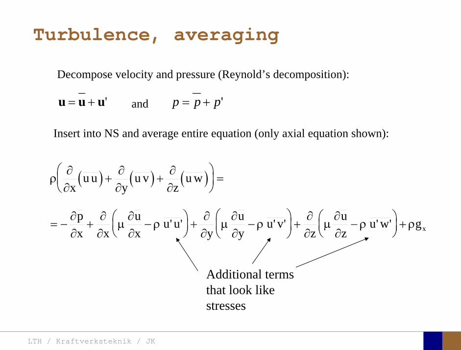
Turbulence, averaging
'uuu += 'ppp +=
Insert into NS and average entire equation (only axial equation shown):
and
Decompose velocity and pressure (Reynold’s decomposition):
( ) ( ) ( )ρ∂∂
∂∂
∂∂
∂∂
∂∂
μ∂∂
ρ∂∂
μ∂∂
ρ∂∂
μ∂∂
ρ ρ
xu u
yu v
zu w
px x
ux
u uy
uy
u vz
uz
u w gx
+ +⎛⎝⎜
⎞⎠⎟ =
= − + −⎛⎝⎜
⎞⎠⎟+ −
⎛⎝⎜
⎞⎠⎟ + −⎛
⎝⎜⎞⎠⎟+' ' ' ' ' '
Additional terms that look like stresses

LTH / Kraftverksteknik / JK
Turbulence, RANS modelling
Reynolds stress tensor
' ' ' ' ' '
' ' ' ' ' ' ' ' ' '
' ' ' ' ' 'ij i j
u u u v u w
R u u v u v v v w
w u w v w w
ρ ρ ρ
⎛ ⎞⎜ ⎟
= − ⊗ = = = ⎜ ⎟⎜ ⎟⎜ ⎟⎝ ⎠
R u u
Needs to be expressed as a function of variables we know or intend to solve for
TURBULENCE MODEL

LTH / Kraftverksteknik / JK
Turbulence
10 unknown:velocity components, pressure and correlations of fluctuating velocity,
4 equations:Averaged momentum equations and averaged continuity equation
' 'u v

LTH / Kraftverksteknik / JK
Turbulence, RANS modelling
R ux
ux
kij Ti
j
j
iij= +
⎛
⎝⎜⎜
⎞
⎠⎟⎟ −μ
∂∂
∂∂
ρ δ23
ερμ μ /2kCT =
⎥⎥⎦
⎤
⎢⎢⎣
⎡⎟⎟⎠
⎞⎜⎜⎝
⎛++−=
kk
T
kl
kkl
kk x
kxx
uR
xku
∂∂
σμμ
∂∂ε
∂∂
∂∂ρ
⎥⎥⎦
⎤
⎢⎢⎣
⎡⎟⎟⎠
⎞⎜⎜⎝
⎛++−=
k
T
kl
kkl
kk xxk
Cxu
Rk
Cx
u∂∂ε
σμμ
∂∂ερ
∂∂ε
∂∂ερ
εεε
2
21
44.11 =εC 92.12 =εC 09.0=μC 1=kσ3.1=εσ
Closure coefficients

LTH / Kraftverksteknik / JK

LTH / Kraftverksteknik / JK
References, turbulence
• Tennekeys and Lumley, “A first course in Turbulence”, MIT Press, 1972.
• J. O. Hinze, “Turbulence”, McGraw-Hill, 1959.• D. C. Wilcox, “Turbulence Modeling for CFD”, DCW Industries, 1998.

LTH / Kraftverksteknik / JK
CFD and experiments
• No, this is not a CFD course, but..• Experiments

LTH / Kraftverksteknik / JK
What do we need to measure?Overall performance
Flow rates (mass or volume)PressureTemperatureShaft power
Performance increase
Separations (velocity)Secondary flows, e.g. tip clearance losses (velocity)Shock waves (supersonic applications)Pressure (resolved in time and space) Temperature (resolved in time and space)

LTH / Kraftverksteknik / JK
Cascade wind tunnels
FIG. 3.1. Compressor cascadewind tunnels. (a) Conventional low-speed, continuousrunning cascade tunnel (adapted from Carter et al. 1950).(b) Transonic/supersoniccascade tunnel (adapted from Sieverding 1985).

LTH / Kraftverksteknik / JK
Closed circuit tunnels

LTH / Kraftverksteknik / JK
components
Settling Chamber
The settling chamber is located between the fan or wide angle diffuser and the contraction and contains the honeycombs and screens used to moderate longitudinal variations in the flow. Screens in the chamber should be spaced at 0.2 chamber diameters apart so that flow disturbed by the first screen can settle before it encounters the second.
Honeycombs
Honeycombs are located in the settling chamber and are used to reduce nonuniformities in the flow. For optimum benefit, honeycombs should be 6-8 cell diameters thick and cell size should be on the order of about 150 cells per settling chamber diameter.

LTH / Kraftverksteknik / JK
components
Screens
Screens are typically located just downstream of the honeycomb and sometime at the inlet of the test section. Screens create a static pressure drop and serve to reduce boundary layer size and increase flow uniformity.
Contraction Section
Contractions sections are located between the settling chamber and the test sections and serve to both increase mean velocities at the test section inlet and moderate inconsistencies in the uniformity of the flow. Large contraction ratios and short contraction lengths are generally more desirable as they reduce the power loss across the screens and the thickness of boundary layers. Small tunnels typically have contraction ratios between 6 and 9.

LTH / Kraftverksteknik / JK
Flow meters with pressure measurement
Venturi-tube
A1 A2
P1 P2
1 1 2 2C A C A=In the incompressible case
2 21 1 2 2
2 2C P C P
ρ ρ+ = +Assuming horisontal mounting

LTH / Kraftverksteknik / JK
Daniel Bernoulli 1700-1782
Daniel Bernoulli was the son of Johann Bernoulli. He was born in Groningen while his father held the chair of mathematics there. His older brother was Nicolaus(II) Bernoulli and his uncle was Jacob Bernoulli so he was born into a family of leading mathematicians but also into a family where there was unfortunate rivalry, jealousy and bitterness.
Undoubtedly the most important work which Daniel Bernoulli did was his work on hydrodynamics. Even the term itself is based on the title of the work which he produced called Hydrodynamica and, before he left St Petersburg, Daniel left a draft copy of the book with a printer. However the work was not published until 1738 and although he revised it considerably between 1734 and 1738, it is more the presentation that he changed rather then the substance.
This work contains for the first time the correct analysis of water flowing from a hole in a container. This was based on the principle of conservation of energy which he had studied with his father in 1720. Daniel also discussed pumps and other machines to raise water. One remarkable discovery appears in Chapter 10 of Hydrodynamica where Daniel discussed the basis for the kinetic theory of gases. He was able to give the basic laws for the theory of gases and gave, although not in full detail, the equation of state discovered by Van der Waals a century later.

LTH / Kraftverksteknik / JK
Venturi-tube (2)
22 2 12 2
2
2A PC CA ρ
⎛ ⎞ Δ− =⎜ ⎟
⎝ ⎠
A1 A2
P1 P2
Solve for e.g. C2:
1 2P P PΔ = −
( )
12
2 2 21 2
21
PCA Aρ
⎛ ⎞Δ⎜ ⎟=⎜ ⎟−⎝ ⎠
and( )
12
2 2 2 2 21 2
21
Pm A C AA Aρρ
⎛ ⎞Δ⎜ ⎟= =⎜ ⎟−⎝ ⎠
where
Flow meters with pressure measurement

LTH / Kraftverksteknik / JK
Flow meters with pressure measurement
Orifice meters
A1
A2
P1 P2
Applicable for pipe flowsSame principle as for VenturiPositioning of pressure taps importantVena contracta and losses require inclusion of Discharge Coefficient, CD
( )
12
2 2 21 2
21D
Pm C AA Aρ⎛ ⎞Δ⎜ ⎟=
⎜ ⎟−⎝ ⎠where ( )1 2Re,DC f A A=
CD available from manufacturer (measurements) or Standards (e.g. ISO)

LTH / Kraftverksteknik / JK
Coriolis flow meter
An actuator (not shown) induces a vibration of the tubes
When there is mass flow, Coriolis forces induce twisting of the tubes
degree of phase-shift is a measure for the amount of mass that is flowing through the tubes

LTH / Kraftverksteknik / JK
Thermal flow meter
Heat is added electrically to the flowTemperature is measured before and after heat addition
pP mC TΔ=

LTH / Kraftverksteknik / JK
Ultrasonic flow meters
Ultrasound is emitted to small particles in the flow (dust or other)Reflections of the sound is frequency shifted by the Doppler effectThe frequency change is proportional to the particles velocity (volume flow meter)

LTH / Kraftverksteknik / JK
Inductive flow metersA magnetic flowmeter is based upon Faraday's Law:
The voltage induced across any conductor as it moves at right angles through a magnetic field is proportional to the velocity of that conductor.
E is proportional to V x B x D where:
E = The voltage generated in a conductorV = The velocity of the conductorB = The magnetic field strengthD = The length of the conductor
N.B: electric conductivity is required

LTH / Kraftverksteknik / JK
Temperature measurements
Thermocouples:
The basis established by Thomas Johann Seebeck in 1821A conductor generates a voltage when subjected to a temperature gradientTo measure this voltage, one must use a second conductor material which generates a different voltage under the same temperature gradient

LTH / Kraftverksteknik / JK
Pressure sensing
1 2p p> 2p p2 may be the atmosphere, a static pressure tap or a known reference pressure
The strain of the diaphragm (or it’s deflection) may be measured by a number of electric methods
Diaphragm

LTH / Kraftverksteknik / JK
Pressure sensingPiezoresistive Strain Gage
Uses the piezoresistive effect of bonded or formed strain gauges to detect strain due to applied pressure.
Capacitive
Uses a diaghragm and pressure cavity to create a variable capacitor to detect strain due to applied pressure.
Magnetic
Measures the displacement of a diaphragm by means of changes in inductance (reluctance), LVDT, Hall Effect, or by eddy current principal.
Piezoelectric
Uses the piezoelectric effect in certain materials such as quartz to measure the strain upon the sensing mechanism due to pressure.
Potentiometric
Uses the motion of a wiper along a resistive mechanism to detect the strain caused by applied pressure.

LTH / Kraftverksteknik / JK
3D, highly instationary (periodic) flowPotentially very high velocities (Supersonic)Large temperature differencesLow accessibility (difficult to probe between rotors)Low turbulence levels in most of the domainVery high turbulence in BL and wakes
Properties of measuring object
Point measurements

LTH / Kraftverksteknik / JK
Conventional or non-optical– Static Pressure Measurements– Total Pressure Measurements
• Multy hole probes
– Total Temperature – Hot Wire Anemometry (HWA)
Optical techniques for Velocity Measurements– Laser Two Focous (L2F)– Laser Doppler Anemometry (LDA)– Particle Image velocimetry (PIV)
Point Measurements

LTH / Kraftverksteknik / JK
Static and total pressure
2 2 21 2 1
2 1 2 2 2C C CP P ρ ρ ρ
− = − =
2 0C =Stagnation point:
C1Static pressuretapPrandtl or Pitot tube
Apply the Bernoulli equation from free stream to stagnation point:
21
2 12CP Pρ
= +or
We can also define a stagnation or total pressure:
( )2
101 1 022
CP P Pρ= + = or
Total pressure = Static pressure + dynamic pressure

LTH / Kraftverksteknik / JK
Static pressure

LTH / Kraftverksteknik / JK
Total Pressure and Temperature
Shrouded Probes
Shrouded Probe
Pitot or Prandtl tube
Sensitive to direction

LTH / Kraftverksteknik / JK
Ludwig Prandtl 1875-1953
Ludwig Prandtl, born at Freising, Bavaria on February 4, 1875, was a German Physicist famous for his work in aeronautics. He qualified at Munchen in 1900 with a thesis on elastic stability and held the position of Professor of Applied Mechanics at Gottingen for forty-nine years (from 1904 until his death there on August 15, 1953). In 1925, Prandtl became the Director of the Kaiser Wilhelm Institute for Fluid Mechanics. His discovery in 1904 of the Boundary Layer which adjoins the surface of a body moving in a fluid led to an understandingof skin friction drag and of the way in which streamlining reduces the drag of airplane wings and othermoving bodies. His work on wing theory, published in 1918 - 1919, followed that of F.W. Lanchester (1902-1907), but was carried out independently and elucidated the flow over airplane wings of finite span. Prandtl's work and decisive advances in boundary layer and wing theories became the basic material of aeronautics. He also made important contributions to the theories of supersonic flow and of turbulence, and contributed much to the development of wind tunnels and other aerodynamic equipment. In addition, he devised the soap-film analogy for the torsion of non-circular sections and wrote on the theory of plasticity and of meteorology.

LTH / Kraftverksteknik / JK
Total Pressure, multy hole
Cobra Probe Yaw Probe
5 Hole Probe

LTH / Kraftverksteknik / JK
5 Hole Probes, Calibration

LTH / Kraftverksteknik / JK
The inherent unsteadiness of the flow within turbomachines

LTH / Kraftverksteknik / JK
Hot Wire Anemometry (HWA)
The heat transfer from a thin (one micron), electrically heated wire can be used to determine velocity.
The resistance of the wire is temperature dependent. Within a small temperature range it can be assumed linear: R = R0+α R0(Tm-T0) where R0 is the resistance at a reference temperature T0 and Tm is the mean wire temperature.
The thermal power induced in the wire is balanced by heat transfer to the surrounding fluid, I2R=hπDL(Tm-T0), where h is the heat transfer coefficient and D and L the diameter and length of the wire, respectively.
E = I R

LTH / Kraftverksteknik / JK
Constant Temperature Anemometry (CTA)
The wire is often placed in a Whetstone bridge. If the output from the bridge is amplified and fed back to the bridge, the resistance of the probe, and thus the temperature, will be held constant. This prevents the temperature of the wire to become excessive at low velocities.
R1
R2 R3
Probe
Bridge Voltage

LTH / Kraftverksteknik / JK
Constant Temperature Anemometry (CTA)

LTH / Kraftverksteknik / JK
Characteristics of LDA (according to Dantec)
Invented by Yeh and Cummins in 1964Velocity measurements in Fluid Dynamics (gas, liquid)Up to 3 velocity componentsNon-intrusive measurements (optical technique)Absolute measurement technique (no calibration required)Very high accuracyVery high spatial resolution due to small measurement volumeTracer particles are required

LTH / Kraftverksteknik / JK
LDA - Fringe Model
Focused Laser beams intersect and form the measurement volumePlane wave fronts: beam waist in the plane of intersectionInterference in the plane of intersectionPattern of bright and dark stripes/planes: Fringes

LTH / Kraftverksteknik / JK
LDA-measuring volume
d
x
x
y
y
z
z
e-2 CONTOUR
FRINGES
κ
κ
κ
κ
De-2
De-2
dml m
a
b
cx
b
z
ya
cd
d
=
=
=
J
J
J
J
JP
JP
JP
JD
JD
JD
+
+
+
a
b
c
d
κπλ
=− sinD
f4l2e
m
κπλ
=− cosD
f4D2e
m

LTH / Kraftverksteknik / JK
Laser Two Focus

LTH / Kraftverksteknik / JK
Laser Two Focus

LTH / Kraftverksteknik / JK
PIV measurements
PIV is a fairly new technique, capable of simultaneous velocity measurements at many points in a plane. This gives information on large scale structures, vorticity etc. which is very difficult or impossible to obtain from one-point measuring techniques.PIV involves the illumination of a plane of the flow under investigation with a thin, pulsed sheet of light. The flow is seeded with particles.The light scattered from the particles and from successive pulses are being recorded either on film or a CCD array, forming a multiple exposure of each particle image. If the time between the pulses is known, velocity can be determined as the ratio of the particle displacement and the elapsed time:
tΔΔ= /xu

LTH / Kraftverksteknik / JK
PIV

LTH / Kraftverksteknik / JK
PIV measurements, illumination
YA
G
YA
G
Two frequency doubled YAG Lasers aligned to one double pulsed laser sheet
Two, or more, separate light pulses can be obtained by chopping a continuous laser or from pulsed lasers.
The limited pulse energies obtained from continuous lasers limits their applicability to low velocity flows or flows where large seeding particles can be used (i.e. liquid flows).
The low repetition rate of most pulsed lasers makes the use of two lasers advantageous.

LTH / Kraftverksteknik / JK
PIV measurements, recording
High seeding density in laminar flame
Film or CCD-camerasCross- or Auto-correlation
– i.e. both particle images on the same frame or on separate frames.
CCD-camera requirement:– A many pixels as possible– 2k by 2k available, 4k, by 4k coming

LTH / Kraftverksteknik / JK
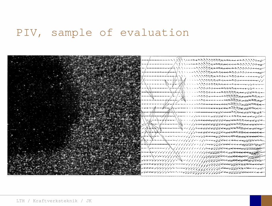
PIV measurements, analyses
Low seeding density: (Number of seeding particles per unit volume)
Each particle image pair can be identified. This is called particle tracking.
High seeding density: (PIV)
Small sub-regions of the image, containing many particle image pairs, are processed to obtain one velocity vector.

LTH / Kraftverksteknik / JK
PIV measurements, analyses

LTH / Kraftverksteknik / JK
PIV measurements, analyses
( ) ( ) ( ) xsxxs dIIR 2A
1
I
+= ∫
Cross correlation between ( )x1I and ( )x2I
s is a two dimensional displacement vector
IA is the interrogation area

LTH / Kraftverksteknik / JK
−10
0
10
−10
0
10
−0.10
0.10.2
0.30.4
pixels
AUTO CORRELATION
−10
0
10
−10
0
10
−0.10
0.10.2
0.30.4
pixels
CROSS CORRELATION
LTH / Kraftverksteknik / JK
PIV, sample of evaluation

LTH / Kraftverksteknik / JK
LDA PIV HWA Velocity range 0.1 mm/s – 300
m/s 0.2 – 150 m/s
Measuring Volume
D = 0.05, L = 0.5 mm
2 by 2 by 0.5 mm
L = 0.5 mm
Freq. response O(10 000) Hz O(10) Hz O(100 000) Hz Calibration Yes No No Sensitivity to other than velocity
Low (ref. Index) Low (ref. Index) Large (temperature, concentrations…)
Continuous Signal
Sometimes Seldom Always
Noise High High Low Turbulence intensity
No limitation Some limitation < 20%
Price O(1 000 000) SEK
O(1 000 000) SEK
O(50 000) SEK
Required Knowledge
High medium Low
Comparison of techniques

LTH / Kraftverksteknik / JK
References, experiments
R. J. Goldstein, “Fluid Mechanics Measurements”, Hemisphere Publishing, 1983.A. V. Johansson & P. H. Alfredsson, “Experimentella metoder inomströmningsmekaniken”, Inst. För Mekanik, KTH.F. Durst, A. Melling and J. H. Whitelaw, “Principals and Practice of Laser Doppler Anemometry”, 1984R. J. Adrian, “Particle-imaging techniques for experimental fluid mechnics”, Ann. Rev. Fluid Mech., 1991.

LTH / Kraftverksteknik / JK
Sample of LDA-measurements
Rotor blade
Glas window
Emitted beams
Scattered Light
Adjustable mirror

LTH / Kraftverksteknik / JK
Axial velocity sorted into 10 bins
0 1 2 3 4 5 6
tangential coordinate (degrees)
-20
0
20
40
60
80
100
120
140
160A
xial
vel
ocity
and
sta
ndar
d de
viat
ion
(m/s
)
radial position: 7 mm from inner window surfaceaxial position: 2.3 mm behind rotor blades

LTH / Kraftverksteknik / JK
Axial velocities in the radial-tangential plane
0
10
20
30
40
50
60
70
80
90
100
2
4
6
8
10
02
46
810
1214
0
20
40
60
80
100
distance from window (mm)
Tangential coordinate (degrees)
Axi
al v
eloc
ity (
m/s
)

LTH / Kraftverksteknik / JK
Airfoils: NACA 4-digit
The NACA four-digit wing sections define the profile by:
One digit describing maximum camber as percentage of the chord.One digit describing the distance of maximum camber from the airfoil leading edge in tens of percents of the chord.Two digits describing maximum thickness of the airfoil as percent of the chord.
Example, the NACA 2412 airfoil has a maximum camber of 2% located 40% (0.4 chords) from the leading edge with a maximum thickness of 12% of the chord.
Four-digit series airfoils by default have maximum thickness at 30% of the chord (0.3 chords) from the leading edge.

LTH / Kraftverksteknik / JK
Airfoils: NACA 4-digit
• c is the chord length• x is the position along
the chord from 0 to c,• y is the half thickness at
a given value of x (centerline to surface)
• t is the maximum thickness as a fraction of the chord

LTH / Kraftverksteknik / JK
Death by PowerPoint