computational fluid dynamics modeling of a …
TRANSCRIPT

COMPUTATIONAL FLUID DYNAMICS MODELING OF A CONTINUOUS TUBULAR
HYDROTHERMAL LIQUEFACTION REACTOR
BY
ZHONGZHONG ZHANG
THESIS
Submitted in partial fulfillment of the requirements
for the degree of Master of Science in Agricultural and Biological Engineering
in the Graduate College of the
University of Illinois at Urbana-Champaign, 2013
Urbana, Illinois
Adviser:
Professor Yuanhui Zhang

ii
ABSTRACT
Fossil fuels are long known for its unsustainability and environmental impact. Therefore,
the search for renewable energy resources has been a persistent effort in both academia and
industry. Amongst a wide variety of candidates, Environmental-Enhancing Energy (E2-Energy)
receives special attention due to the incorporation of energy production, carbon dioxide capture,
and wastewater treatment. Hydrothermal liquefaction (HTL) is the key component in the
technology. It involves the conversion of biowaste and algae into hydrocarbon fuels at elevated
temperature and pressure. However, E2-Energy is not yet commercially feasible due to a lack of
reliable, up-scaled HTL equipment despite its promising prospective. Improving the efficiency of
the hydrothermal conversion is an effective way of increasing the economic viability and
benefits of the technology. Tubular continuous reactors are generally considered to be favorable
for HTL due to the continuous production and the aptitude for scale-up. Recently, a bench scale
tubular continuous reactor system has been developed at the University of Illinois.
As HTL is sensitive to the reacting environment, it is crucial to understand the velocity
and temperature distributions, heating uniformity, and heat transfer efficiency within the reactor.
However, the high pressure and temperature of HTL process make it difficult to conduct direct
measurements of these parameters. A numerical investigation is an appropriate alternative. The
objective of this study is to develop a computational fluid dynamics (CFD) model using
commercial code ANSYS FLUENT to examine the adequacy of the current design. The model
takes inputs of operating temperature of the reactor, temperature of the feedstock reservoir, and
residence time, and outputs various parameters including the velocity and temperature profiles
and Nusselt number.

iii
The flow regime is best characterized as a turbulent mixed convection. Therefore, shear
stress transition k model with low-Reynolds-number correction is chosen because it is able
to resolve the turbulence features and at the same time preserve the buoyancy-induced flow
pattern. A representative test is run using water as the feedstock with the input parameters being
300 °C, 25 °C, and 30 min, respectively. Typical mixed convection characteristics are observed:
symmetric secondary vortex within the cross-section perpendicular to the tube axis and
temperature stratification. In addition, Nusselt number in the fully developed region is
significantly higher than that of Poiseuille flow, indicating an enhanced heat transfer rate. The
residence time distribution is also found to noticeably deviate from typical laminar flow. The
mean retention time is shortened by about 60 seconds for a total of 300 seconds due to the
variation of velocity in the heated zone. A correction method is proposed to account for this
accelerating effect.
Finally, the model is validated by virtually replicating Mori’s experiment (Mori et al.
1966). The computational prediction and experimental measurement show satisfactory
agreement.

iv
ACKNOWLEDGEMENTS
First I would like to thank my advisor, Professor Yuanhui Zhang for his guidance and
encouragement throughout my academic career at the University of Illinois. I also would like to
appreciate Doctor Yigang Sun and Professor Lance Schideman for serving on my defense
committee.
I wish to extend my acknowledgement to my friend Doug Barker, who helped me in
numerous aspects of my graduate study. Last but not least, my special thanks go to my family for
their unconditional love and support.

v
Table of contents
List of figures.......................................................................................................................... vii
List of tables .......................................................................................................................... viii
Nomenclature ...........................................................................................................................ix
CHAPTER 1 Introduction ........................................................................................................ 1
1.1. Energy .................................................................................................................................... 1
1.2. Microalgae biomass ................................................................................................................ 1
1.3. Hydrothermal liquefaction .................................................................................................... 3
1.4. Reactor design ........................................................................................................................ 4
1.5. Objectives ............................................................................................................................... 4
CHAPTER 2 Literature review ................................................................................................ 6
2.1. Mixed convection heat transfer ............................................................................................. 6
2.1.1. Effect of buoyancy force ................................................................................................. 7
2.1.2. Laminar to turbulent transition ................................................................................... 12
2.2. Residence time distribution.................................................................................................. 14
CHAPTER 3 Materials and methods ..................................................................................... 16
3.1. Computational fluid dynamics ............................................................................................. 16
3.1.1. Governing equations..................................................................................................... 16
3.1.2. Finite volume method ................................................................................................... 18
3.1.3. Discretization scheme ................................................................................................... 19
3.1.4. Buoyancy-driven flows ................................................................................................. 21
3.1.5. Turbulence model ......................................................................................................... 21
3.1.6. Numerics ....................................................................................................................... 23
3.2. Geometry .............................................................................................................................. 24
3.3. Mesh ..................................................................................................................................... 26
3.4. Boundary condition .............................................................................................................. 28
3.5. Materials ............................................................................................................................... 30
CHAPTER 4 Validation case .................................................................................................. 32
CHAPTER 5 Results and discussion ...................................................................................... 36
5.1. Heat exchanger ..................................................................................................................... 36
5.2. Velocity and temperature profiles ....................................................................................... 38
5.3. Nusselt number..................................................................................................................... 44

vi
5.4. Effect of tube orientation ..................................................................................................... 46
5.4.1. Velocity and temperature ............................................................................................. 46
5.4.2. Nusselt number ............................................................................................................. 48
5.4.3. Inclined tube ................................................................................................................. 49
5.5. Residence time distribution.................................................................................................. 51
5.6. Mesh independence study .................................................................................................... 54
CHAPTER 6 Conclusions and recommendations.................................................................. 56
6.1. Conclusions........................................................................................................................... 56
6.2. Recommendations ................................................................................................................ 58
References ............................................................................................................................... 60
Appendix A Physical properties of fluids ............................................................................... 65

vii
List of figures
Figure 3.1 Schematic diagram of the reactor geometry (all parts included) ................................ 25 Figure 3.2 Mesh of the heat exchanger (from the top are: shell, cold fluid, tube, and hot fluid) .. 26 Figure 3.3 Mesh of the reactor in the cross-section perpendicular to tube axis ........................... 27 Figure 3.4 Mesh spacing contrast at the transition between heated and unheated zones (right is
the heated zone) ........................................................................................................................ 28 Figure 3.5 Schematic flow chart of the feedstock and product ................................................... 29 Figure 3.6 Density of water as a function of temperature ........................................................... 30 Figure 4.1 Wall temperature along the axial direction (Mori et al. 1966) ................................... 33 Figure 4.2 Dimensionless velocity along vertical center-line at 6 m (Mori et al. 1966) .............. 34 Figure 4.3 Dimensionless temperature along vertical center-line at 6 m (Mori et al. 1966) ........ 34 Figure 5.1 Outlet temperature and the energy recovery ratio under various operating
temperatures .............................................................................................................................. 37 Figure 5.2 Temperature of cold and hot fluids in the heat exchanger along center-lines,
respectivley ............................................................................................................................... 38 Figure 5.3 Centerline temperature and mean temperature in the axial direction ......................... 39 Figure 5.4 Velocity vectors in the heated zone from 10 in to 20 in (reversed flow in the upper
half) .......................................................................................................................................... 40 Figure 5.5 Velocity distributions along the vertical center-line at three locations in the heated
zone .......................................................................................................................................... 40 Figure 5.6 Streamlines in the cross-section at z = 15 in showing the secondary vortices due to
natural convection ..................................................................................................................... 41 Figure 5.7 Temperature contours on symmetric plane in the heated zone from 10 in to 20 in ..... 42 Figure 5.8 Temperature distribution along the vertical center-line at three locations in the heated
zone .......................................................................................................................................... 43 Figure 5.9 Stratified temperature contours in the cross-section z = 15 in .................................... 43 Figure 5.10 Nusselt number around azimuth at three locations in the heated zone ..................... 45 Figure 5.11 Velocity and temperature distributions in the fully developed region for upward flow
................................................................................................................................................. 47 Figure 5.12 Velocity and temperature distributions in the fully developed region for downward
flow .......................................................................................................................................... 48 Figure 5.13 Velocity profile along the vertical centerline at 15 in for inclined downward, inclined
upward, and horizontal flows .................................................................................................... 50 Figure 5.14 Temperature profile along the vertical centerline at 15 in for inclined downward,
inclined upward, and horizontal flows ....................................................................................... 51 Figure 5.15 Residence time distribution for 6-feet tube ............................................................. 52 Figure 5.16 Residence time distribution with corrected inlet velocity ........................................ 54 Figure 5.17 Velocity profile at z = 15 in for coarse and refined mesh ........................................ 55 Figure 5.18 Temperature profile at z = 15 in for coarse and refined mesh .................................. 55

viii
List of tables
Table 3.1 Detailed numerical methods used in the simulation .................................................... 23 Table 3.2 Cross sectional dimensions of the heat exchanger ...................................................... 24
Table 3.3 Boundary conditions of the simulation ....................................................................... 30 Table 4.1 model setup for the validation case ............................................................................ 32
Table 5.1 Nusselt numbers of fully developed horizontal mixed convection .............................. 45 Table 5.2 Nusselt numbers of fully developed upward and downward flow ............................... 48
Table 5.3 Residence distribution time parameters ...................................................................... 52
Table A.1 Properties of saturated water ..................................................................................... 65
Table A.2 Properties of air at 1 atm pressure ............................................................................. 66

ix
Nomenclature
Gr = Grashof number, 3
2
w mg T T D
Re = Reynolds number, mw D
Ri = Richardson number, 2
Gr
Re
Pr = Prandtl number,
Ra = Rayleigh number, Gr Pr
Pe = Peclet number, Re Pr
Nu = Nusselt number, hD
k
g = gravitational acceleration, m/s2
β = thermal expansion coefficient, 1/K
T = temperature, °C
ν = kinematic viscosity, m2/s
α = thermal diffusivity, m2/s
D = tube diameter, m
r = radial distance, in
R = tube radius, in
w = axial velocity, m/s
h = heat transfer coefficient, W/(m2·K)
k = thermal conductivity, W/(m·K)

x
θ = dimensionless temperature, w
w c
T T
T T
W = dimensionless axial velocity, c
w
w
ṁ = mass flow rate, kg/s
sq = surface heat flux, W/m2
τ = residence time, s
z = axial distance from the inlet, in
η = energy recovery ratio of the heat exchanger
Subscripts
w = value at the tube wall
c = value at the tube center
m = mean value of the cross section
1
CHAPTER 1
Introduction
1.1. Energy
In 2010, the U.S. annual energy consumption was 98.0 quadrillion Btu. Fossil fuels
accounted for 83.0% of the total consumption, with petroleum 36.7%, natural gas 25.1%, and
coal 21.2%. Meanwhile, 30.6% of the total energy consumption and 49.2% of petroleum
consumption were imported, respectively (USDOE 2011). The reliance on import leads to a
potential threat on energy security. Also, fossil fuels are known for being subject to limited
amount of reserves and thus not sustainable. Moreover, the environmental impact of fossil fuels,
such as increased greenhouse gas levels, raises a global concern about their usage. Therefore, it
is of great importance to seek alternative (renewable and carbon-neutral) energy resources.
1.2. Microalgae biomass
Biomass refers to all organic matter that stems from plants, including aquatic and
terrestrial. As a result of photosynthesis by these plants, biofuels derived from biomass have
significantly reduced net carbon dioxide emission. Due to the capability of mitigating
greenhouse gas emission, conversion of biomass has been given great research attention
worldwide.
First generation biofuels have been based on extraction from sugar and starch crops
(ethanol) and oilseed crops (biodiesel) (FAO 2008). The production of first generation biofuels,
however, brought great controversy, due to the competition with food production for the use of
arable land. For this reason, the potential of replacing fossil fuels by first generation biofuels
remains limited. Currently, the production of first generation biofuels only contributes to 1% of
global transport fuels (Brennan and Owende 2010).

2
The development of second generation biofuels has focused on lignocellulosic biomass
derived from whole plant matter of designated energy crops or agricultural, forest, and wood
processing residues (Moore 2008). Although it resolve the conflict between food production and
fuel generation, second generation biofuels are still far from commercial-scale exploitation
because cellulosic biomass is more resistant to being broken down than starch, sugar and oils,
which makes the conversion into liquid fuels more expensive (FAO 2008).
From the first and second generation biofuels, we can abstract the ideal characteristics for
a technically and economically feasible biofuel resource: it should demand minimum amount of
arable land; should produce abundant biomass within short duration of time; should mitigate
global warming; and, should be competitive to fossil fuels in price. Successful employment of
microalgae can meet these requirements.
Microalgae consist of a wide range of unicellular and simple multi-cellular
microorganisms, including cyanobacteria (Chloroxybacteria), green algae (Chlorophyta), red
algae (Rhodophyta), and diatom (Bacillariophyta) (Brennan and Owende 2010). The advantages
of using algae as a biofuel feedstock are: (1) microalgae have a higher photosynthetic efficiency
and faster growth rate than terrestrial plants, they can double the biomass in as short as 3.5h
during exponential growth period (Chisti 2007; Singh and Dhar 2011); (2) microalgae can be
grown and harvested all year round; (3) the lipid content in microalgae typically ranges from
20% to 50% on a dry weight basis, exceeding 80% in some species (Spolaore et al. 2006;
Metting Jr. 1996), consequently, biodiesel yield per area of microalgae is much higher than that
of rapeseed (Schenk et al. 2008); (4) microalgae can be cultivated on non-arable lands,
minimizing the impact on food production (Searchinger et al. 2008); (5) algal biofuels are carbon
neutral, as producing 1kg of algae biomass fixes about 1.83kg of carbon dioxide (Chisti 2007);

3
(6) microalgae can remove nitrogen and phosphorus from wastewater, therefore, microalgae
cultivation can be coupled with wastewater treatment (Cantrell et al. 2008); (7) microalgae
biomass also produces valuable co-products such as protein, in addition, the residue after oil
extraction can be used as animal feed and fertilizer (Spolaore et al. 2006), or generate ethanol
and methane by fermentation (Hirano et al. 1997).
1.3. Hydrothermal liquefaction
Currently, microalgae are most commonly utilized as the feedstock of biodiesel
production. The process involves the extraction of triglycerides from algal biomass and the
subsequent conversion (via transesterification) into biodiesel. This approach requires drying of
the algal biomass and extraction using organic solvents. These steps add considerable cost to the
process. An alternative method that needs no drying or organic solvents is hydrothermal
conversion. The approach converts moist microalgae paste in aqueous media at elevated
temperature and pressure. Liquefaction is performed at temperatures below the critical point of
water and liquid bio-crude oil that primarily consists of hydrocarbons is the desired product.
Studies of hydrothermal liquefaction have been conducted under various parameters with a
number of microalgae species (Dote et al. 1994; Sawayama et al. 1995; Kishimoto et al. 1994;
Yang et al. 2004). It was conclude that the oil yield and quality vary significantly with respect to
temperature, retention time, catalyst, and microalgae strains. Typically, hydrothermal
liquefaction is carried out at temperatures between 200~300 °C for 30~60 minutes with or
without alkali catalyst. Oil yields range from 33 to 64 wt %. Heating values of the bio-crude are
usually 28~50 MJ/kg. In addition, Minowa et al. (1995) and Sawayama et al. (1999) analyzed the
ratio of energy input and output of microalgae liquefaction and suggest that the process is a net
energy producer.

4
1.4. Reactor design
Bench scale hydrothermal liquefaction experiments are typically conducted in batch
autoclaves. One of the shortcomings of autoclaves is relatively low heat transfer rate and high
thermal inertia (Knezevic 2009). As a result, considerable amount of reactions occur during the
prolonged heating/cooling time (Fang et al. 2004; Watanabe et al. 2005). Therefore conventional
autoclave reactors are not suitable for HTL kinetics and mechanism studies. Additionally,
elongated heating and cooling period severely limits their application in commercial scale
production. Continuous systems, on the other hand, enjoy several advantages including high
throughput, steady state operation, and easy scale-up. Considering the benefits, we recently
developed a bench-scale, continuous, tubular hydrothermal liquefaction reactor. Generally, three
assumptions are made in most studies on tubular reactors: ideal plug flow and no axial mixing;
complete radial mixing; and uniform velocity and temperature profiles across the radius. Various
parameters may then be readily derived. The assumptions, however, may not be applicable to all
applications, especially those with such extreme operating conditions as hydrothermal
liquefaction. Consequently, a closer examination is warranted.
1.5. Objectives
It is of great interest to understand the hydrodynamic and thermal characteristics of the
new-designed tubular plug-flow reactor, since oil yield and quality are directly influenced by
reaction temperature and retention time. However, due to the difficulty of directly measuring the
temperature and velocity within the tube, computational fluid dynamic analysis is employed.
Therefore, this study intends to investigate the heat transfer performance of the reactor using a
commercially available computational fluid dynamic code ANSYS-FLUENT. The detailed
objectives are proposed:

5
1. Examine the effectiveness of the designed length of the heat exchanger and find out
the heat recovery ratio;
2. Define the flow regime within the reactor and apply appropriate model to discover the
velocity and temperature profiles;
3. Study the effect of tube orientation on the flow field and heat transfer;
4. Analyze the residence time distribution.

6
CHAPTER 2
Literature review
2.1. Mixed convection heat transfer
Laminar convective heat transfer is encountered in a wide variety of engineering
application and thus is very well studied both analytically and experimentally. Most studies,
however, are limited to pure forced convection where constant properties of fluid are assumed.
Since the density of most fluids is dependent on temperature, the assumption is valid only when
the temperature change is sufficiently small so that the magnitude of natural convection is
negligible compared to that of forced convection. As a matter of fact, both mechanisms are of
comparable order of magnitude in many practical situations. Such flow is usually termed mixed
convection or combined convection flow.
The relative magnitude of free and forced convection may be obtained from a study of
dimensionless parameters. Richardson number describes the importance of buoyancy force in a
mixed convection flow. It is the ratio of Grashof number to the square of Reynolds number.
2 2Re
w mg T T LGrRi
u
(2.1.1)
where g is the gravitational acceleration, is the thermal expansion coefficient, wT is
the wall temperature, mT is the mean temperature, L is the characteristic length, and u is mean
velocity.
Typically, forced convection is predominant whereas natural convection is negligible
when Ri <0.1; natural convection is predominant whereas forced convection is negligible when
Ri >10; and neither is negligible when 0.1< Ri <10. Still, it is sometimes difficult to draw a clear
distinction between the two effects and arbitrary criteria are necessary. For instance, Metais and

7
Eckert (1964) arbitrarily defined mixed convection as the actual heat flux deviated more than 10
percent from that by either pure forced convection or pure free convection.
Strong influence of buoyancy force can be expected in the current system due to the low
velocity and the high heat flux.
2.1.1. Effect of buoyancy force
A number of studies investigated the effect of buoyancy force with various configurations,
including working media, tube orientation, dimensionless numbers, etc. It is generally concluded
that the velocity and temperature profiles are markedly different from their counterpart for pure
forced convection. A significant increase of Nusselt number is also typically observed. This
section summarizes the relevant literature studies on this topic.
2.1.1.1. Velocity and temperature profile
Velocity and temperature profiles at cross-sections perpendicular to tube axis can be
readily derived by solving governing equations for laminar flow and energy balance. The results
are independent of tube orientation when gravity is ignored. In mixed convection, however, the
inclination of tube axis significantly influences motion and heat distribution, two limiting cases
being: vertical tuber and horizontal tube. In vertical tubes buoyancy force is parallel to the
direction of flow; thus it is still possible to analytically solve the governing equations for
momentum and energy and the solution remains axisymmetric about the tube axis. In horizontal
tubes, on the other hand, buoyancy force and externally forced flow are perpendicular to each
other; the absence of axial symmetry considerably increases the mathematical difficulty in
solving the fluid motion. Therefore, various attempts were made using experimental, analytical,
and numerical methods.

8
Mori et al. (1966) experimentally studied the effect of buoyancy force on the velocity and
temperature fields of the fully developed flow of air in a uniformly heated horizontal tube.
Velocity and temperature were measured by calibrated, cylindrical yaw probes and T-shaped
thermocouples traversing the tube, respectively. They concluded that because wall temperature
was higher than the bulk fluid temperature, the fluid near the wall was heated and moved upward
along the wall due to buoyancy, while the fluid in the center was cooler and thus descended. As a
result, a secondary flow that was symmetric about the vertical plane passing through the tube
axis was formed. Due to this effect, velocity and temperature distributions were found to
evidently differ from those of Poiseuille flow. Instead of the parabolic shaped, velocity and
temperature profiles were concave downward in vertical direction whereas remained symmetric
in horizontal direction. In the follow-up report (Mori and Futagami 1967), they observed the
secondary flow described above by injecting NH4CL smoke in a transparent tube. It was also
pointed out that the dimensionless velocity profile was relatively independent of Ra , while the
dimensionless temperature profile concaved further downward with increasing Ra .
Siegwarth and Hanratty (1970) investigated the stream function and velocity and
temperature distributions of a high Prandtl number fluid – ethylene glycol – in a heated
horizontal tube by experimental and computational methods. The measured and calculated
temperature profile showed good qualitative accordance with Mori’s data. Stream functions
computed by finite difference method also agreed well with Mori’s visualization. However,
velocity profile remained close to a parabolic shape due to large Prandtl. In addition, maximum
velocity appeared above the horizontal axis in contrast to Mori’s observation. The trend was
attributed to the decrease of viscosity with height in the tube due to the increase in temperature,
whereas the viscosity of air stayed relatively constant with temperature.

9
Given the fact that no exact solution exist for mixed convection flow in horizontal tubes,
perturbation method is a common approach in theoretical studies. The method starts from the
exact solution of pure forced convection, and adds natural convection as a perturbation term to it
to obtain an approximate solution. Morton (1959) hypothesized that the motion due to buoyancy
can be regarded as a secondary flow that modified the main flow by creating a circulation of the
fluid in a direction normal to the tube axis. He then obtained the solutions for the velocity and
temperature in the fully developed region as power series of Ra Re . The solutions had the
following general form:
2
1 2 ...A A (2.1.2)
2
0 1 2 ...W W AW A W (2.1.3)
2
0 1 2 ...A A (2.1.4)
where , W , and are stream function, axial velocity and temperature, respectively,
and A is Rayleigh number. 0W and 0 represent the case of pure forced convection.
Faris and Viskanta (1969) used 2/Gr Re as the perturbation parameter to study a laminar
combined free and forced convection flow within a horizontal circular tube subject uniform heat
flux at the wall. Flow was assumed fully developed and fluid properties were considered
constant except for density in the body force term of momentum equation. The predictions of
velocity and temperature profiles agreed well with the experimental data by (Mori et al. 1966).
The perturbation approximation, however, is restricted to low Rayleigh number flows and gives
unrealistically high estimate of Nusselt number for 3000ReRa (Bergles and Simonds 1971;
Mori et al. 1966; Mori and Futagami 1967).
Mori and Futagami (1967) employed the boundary layer theory to derive analytical
expression of flow and temperature fields in a mixed convection flow at high Ra values. A

10
boundary layer sufficiently thin compared to the tube radius was assumed. Solutions were then
solved in the core region where secondary velocity was assumed to be uniformly downward and
the boundary layer separately. The results were concluded to be applicable in the range of
410Re Ra and showed good consistency with their previous report (Mori et al. 1966).
A numerical analysis was carried out by (Wang et al. 1994). The governing equations of
continuity, momentum and energy with the Boussinesq approximation were solved by finite
difference method. Various combinations of Pr and Ra were tested and it was discovered that
flow reversal would happen near the top of tube wall with low Pr and high Ra . A Pe Ra
coordinate was given to predict regime of reverse flow occurrence. Similar backflow
phenomenon was also observed by Mikesell for flows with 2
150NuGr
PrRe (Mikesell 1963).
2.1.1.2. Nusselt number correlation
Nusselt number indicates the relative importance of convective and conductive heat
transfer. For fully developed laminar flow in circular tubes with uniform surface heat flux, it is
well known that 48
11Nu
(Cengel 2007). This prediction is limited to pure forced convection
and is found to be inaccurate as buoyancy has a significant impact on the heat transfer rate even
at very low temperature gradient (Morton 1959; Mori et al. 1966). In many studies, the heat
transfer coefficient was found to be considerably higher than indicated in elementary theory due
to the secondary flow. Plenty of efforts have been devoted to establishing a correlation of Nusselt
number and the degree of natural convection.
In his perturbation model (Morton 1959), Morton also gave a prediction to Nusselt
number. As with the velocity and temperature fields, solution was given as power series of the
perturbation parameter RaRe :

11
2
26 1 0.0586 0.0852 0.2686 ...4608
RaReNu Pr Pr
(2.1.5)
Ede (1961) published one of the earliest reports about the effects of natural convection on
laminar flow of water under uniform heat flux boundary condition. Seven pipes of inner diameter
ranging from 0.5 to 2.0 inches were tested, with Reynolds number and Grashof number varying
from 300 to 105 and 10
4 to 10
7, respectively. Thermocouples were attached to a series of
positions along the tube with each position having five thermocouples around the periphery.
Calculations were based on the average value at each distance. The correlation was given as:
0.34.36 (1 0.06 )Nu Gr (2.1.6)
However, the absence of Reynolds number and Prandtl number in Ede’s correlation was
questioned (Kupper et al. 1969). It was suggested that Nusselt number be a function of Reynolds,
Prandtl and Grashof numbers. A correlation was presented based on a series of experiments of
similar setup:
1 51 348
0.04811
Nu Pr ReRa (2.1.7)
Mori (1966) calculated local Nusselt number based on measurements of velocity and
temperature at a cross-section and proposed the following correlation:
1 5
1 5
1.80.61 1Nu ReRa
ReRa
(2.1.8)
The prediction agreed very well with their experimental data. However, this formula was
applicable to fluids of Prandtl number around unity as air was used as the working fluid.
Alternative to correlation formulae, correlation plots of various variables were also
reported. Shannon and Depew (1968) carried out an experimental investigation of free
convection effect. Water was introduced into the test system at ice point. Nusselt number,

12
Reynolds number, and Grashof number were calculated based on local average. Reynolds
numbers ranged from 120 to 2300, and Grashof number reached as high as 2.5×10⁵. A
correlation plot of GzNu Nu vs.
14
Gz
GrPr
Nu was obtained, where
GzNu is the theoretical value
for Poiseuille flow.
Newell and Bergles (1970) solved the governing equations for two limiting cases by
central finite difference scheme: infinite-conductivity tube wall and glass tube wall. They
represented the upper and lower bound to the average Nusselt number estimate, respectively. The
correlation of fully developed Nusselt number with Grashof-Prandtl number product was
presented. In the follow-up study (Bergles and Simonds 1971), the data were combined with the
analysis of transition region to derive a comprehensive prediction of Nusselt number along the
tube axis (x L
RePr) at various Rayleigh and Prandtl numbers.
2.1.2. Laminar to turbulent transition
It is necessary to examine the transition in convective heat transfer flow as the heat
transfer coefficient of turbulent flow differs significantly from that of laminar flow. While the
criterion for transition of forced convection flow from laminar to turbulent is universally agreed
(Cengel 2007), that for mixed convection is much less understood.
In their report (Mori et al. 1966), critical Reynolds number was proposed as a
measurement of turbulence level. The authors concluded that when the turbulence level at the
entrance was high, the secondary flow suppressed the turbulence. As a result, critical Reynolds
number increased with Rayleigh number. In contrast, when the flow at the inlet was laminar, the
secondary flow acted as turbulence. Therefore, critical Reynolds number decreased with
Rayleigh number. The formulae for the above two cases were give as, respectively:
13
1 4
128crRe ReRa (2.1.9)
57700 / 1 0.14 10crRe Re Ra (2.1.10)
Nagendra (1973) investigated the interaction of combined natural and forced convection
in the transition regime of a horizontal tube under uniform heat flux using water. Velocity,
temperature, and pressure drop across the test section were recorded over time to detect
fluctuations as an indicator of turbulence. The effects of velocity and heat flux on the transition
were studied separately by fixing the heat input while changing velocity and keeping the velocity
constant while varying heat flux, respectively. It was found that hydrodynamic and thermal
turbulence occurred separately. These two regimes merged at sufficiently high Reynolds and
Rayleigh number, resulting in turbulent mixed convection. A plot of boundaries of laminar,
transition, and turbulent flow regimes were given.
El-Hawary confirmed Nagendra’s hypothesis by applying similar method to air (El-
Hawary 1980). The author found that the transition due to hydrodynamic effects occurred at
values of GrPr that were little dependent on Re . Similarly, laminar flow became thermally
disturbed at a relatively constant value of RaPr for all Reynolds number. The author also
noticed that there was a disturbed regime that was practically similar to laminar flow. Further
increasing the flow rate, the wall heat flux, or both would cause the flow to enter a short
transition period and then turbulent regime. Unlike Nagendra, however, El-Hawary concluded
that both thermal turbulence and hydrothermal turbulence were of the same nature in a sense that
they were characterized by similar velocity and temperature fluctuations and markedly increased
Nusselt number than laminar flow. Consequently, no subdivision was intended for the turbulent
flow zone in the flow regime map presented.

14
2.2. Residence time distribution
In ideal tubular reactors, where plug-flow is assumed, all molecules of species reside
within the reactors for exactly the same amount of time. In reality, however, nonideal flow
patterns widely exist, resulting in a distribution of residence time of materials within the reactors.
It is of great importance to investigate the residence time distribution (RTD) to understand the
mixing characteristics in a chemical reactor.
Historically, RTD is determined experimentally by injecting a pulse of inert tracer into
the reactor at time 0t , and then monitoring the tracer concentration in the effluent as a
function of time C t . A series of parameters may then be derived from C t (Fogler 1999):
Residence time distribution function E t :
0
C tE t
C t dt
(2.2.1)
Cumulative distribution function F t :
0
t
F t E t dt (2.2.2)
Mean residence time mt :
0
mt tE t dt
(2.2.3)
Variance 2 :
2
2
0mt t E t dt
(2.2.4)
Skewness 3s :
3
3
3 2 0
1ms t t E t dt
(2.2.5)

15
Residence time distribution function describes in a quantitative manner how much time
different fluid elements have spent in the reactor; cumulative distribution function measures the
fraction of the exit stream that has resided in the reactor for a period of time shorter than a given
value t; mean residence time quantifies the average time the effluent molecules spent in the
reactor; the magnitude of variance is an indication of the spread of the distribution; and the
magnitude of skewness assesses the extent that a distribution is skewed in one direction or
another in reference to the mean.

16
CHAPTER 3
Materials and methods
3.1. Computational fluid dynamics
Computational fluid dynamics utilizes numerical methods and algorithms to solve
equations governing fluid flow and heat and mass transfer. Commercial CFD package ANSYS
FLUENT is used in this thesis work.
FLUENT is capable of analyzing a wide range of fluid flow problems including
incompressible and compressible flows, laminar and turbulent flows, viscous and inviscid flows,
Newtonian and non-Newtonian flows, single-phase and multi-phase flows, etc. In addition, both
steady-state and transient analyses can be performed.
In addition, FLUENT provides solution to heat and mass transfer problems. Conduction
and convection can be easily implemented by adding one extra energy equation. Various models
are available to simulate more complex phenomena involving radiation. Species transport can be
modeled by solving equations governing convection, diffusion and reaction.
3.1.1. Governing equations
FLUENT analyzes fluid flow problems by numerically solving governing equations. For
all flows, conservation equations for mass and momentum are solved. For flows involving heat
transfer, additional equation for energy conservation is solved. Turbulence models solve
additional transport equations for turbulent variables. For flows involving mass transfer, a
species conservation equation is solved. Multiphase simulation requires additional equations for
each phase.
3.1.1.1. Mass conservation
The equation for mass conservation is described by:

17
m
St
(3.1.1)
where mS is the source term added to the continuous phase from dispersed second phase
or user-defined sources.
3.1.1.2. Momentum conservation
Momentum conservation equation can be written as follows:
p g Ft
(3.1.2)
where p is the static pressure, is the stress tensor, g is the gravitational body force,
and F is external forces including user-defined source terms.
The stress tensor is defined as:
T 2
3I
(3.1.3)
where represents the molecular viscosity, I is the unit tensor.
3.1.1.3. Energy conservation
Energy conservation equation in FLUENT is given by:
effeff j j h
j
E E p k T h J St
(3.1.4)
The first three terms on the right-hand side stands for energy transfer due to conduction,
species diffusion, and viscous dissipation, respectively, where effk is the effective conductivity
(sum of thermal conductivity k and turbulent conductivity tk given by the turbulence model
used), and jJ is the diffusion flux of species j .
The total energy E in Equation 3.1.4 is written by:

18
2
2
pE h
(3.1.5)
where sensible enthalpy h is defined for ideal gas as:
j j
j
h Y h (3.1.6)
and for incompressible fluid as:
j j
j
ph Y h
(3.1.7)
where jY is the mass fraction of species j and
,ref
T
j p jT
h c dT (3.1.8)
in which refT is 289.15 K.
3.1.1.4. Species transport equations
When species transport model is activated, FLUENT solves a convection-diffusion
equation for each species to predict their local mass fraction:
i i i i iY Y J R St
(3.1.9)
where the second term on the left hand side represents convective transport, iJ is the
diffusion flux of species i due to concentration and temperature gradient, iR is the net
generation rate of species i by chemical reaction, and iS is the source term from the dispersed
phase and any user-defined source.
3.1.2. Finite volume method
Finite volume method (FVM) is a numerical method for discretizing partial differential
equations. It is widely used in commercial CFD codes including FLUENT. In FVM, the domain

19
is divided into a number of control volumes (cells, elements) where the variable of interest is
evaluated at the centroid of the control volume. Volume integral is performed and converts the
divergence term in the partial differential equation (Equation 3.1.10) into a surface integral
(Equation 3.1.11) using divergence theorem. The surface integral is then evaluated as flux at the
surface of each control volume. The flux entering a certain volume is equal to that leaving the
adjacent volumes. Therefore, FVM is inherently conservative by construction.
( ) 0u
f ut
(3.1.10)
0i iV V
udx f n dst
(3.1.11)
where in represents the unit vector outward normal to V .
3.1.3. Discretization scheme
Due to the conversion to surface integral form, face values are required for the
convection and diffusion terms in Equation 3.1.9. However, ANSYS FLUENT stores discrete
values at the cell centroid. Therefore, face values must be interpolated from the cell center. The
diffusion terms are interpolated using central-difference scheme and are always second-order
accurate. The interpolation of the convection terms is accomplished by an upwind scheme.
ANSYS FLUENT offers several choices: first-order upwind, second-order upwind, power law,
and QUICK.
3.1.3.1. First-order upwind
First-order upwind assumes that the cell-center values of any field variable represent a
cell-average value and the face quantities are identical to the cell quantities. Therefore, the face
value f is directly replaced by the cell-center value of variable in the upstream cell. Such
interpolation is first-order accurate.

20
f (3.1.12)
3.1.3.2. Second-order upwind
Higher-order of accuracy can be achieved at cell faces via a Taylor series expansion of
the cell-center solution about the upstream cell centroid. The face value is calculated by the
following expression:
f r (3.1.13)
is the gradient of the quantity in the upstream cell and r is the displacement vector
from the upstream cell centroid to the current cell face centroid.
3.1.3.3. Central difference
The second-order accurate central difference scheme takes average from both upstream
and downstream cells. It computes the face value as follows:
1 1
2 2U Df U U D Dr r (3.1.14)
This scheme is provides improved accuracy for Large Eddy Simulation but can produce
non-physical solutions.
3.1.3.4. QUICK
QUICK scheme is a weighted average of second-order upwind and central difference,
which can be give as:
, ,1f f CD f SOU (3.1.15)
0 results in a second-order upwind scheme, while 1 yields a central difference
interpolation. The implementation in ANSYS FLUENT uses a variable, solution-dependent
value of . The QUICK scheme is generally more accurate on structured meshes where unique
upstream and downstream cells can be identified.

21
3.1.4. Buoyancy-driven flows
When the flow is dominated by buoyancy force, e.g. natural convection, it can be
modeled in ANSYS FLUENT by various methods that approximate density variation with
respect to temperature. The ideal gas law describes the relationship between the density of a gas
and temperature at a given pressure. It has satisfactory accuracy for gaseous flows with small
pressure change. For liquids, the Boussinesq approximation is frequently used thanks to the
relatively fast convergence rate. The model regards density as a constant quantity in all
governing equations to be solved, except for the body force term in the momentum equation:
0 0 0g T T g (3.1.16)
In the above equation, 0 is the constant density of the flow, 0T is the operation
temperature, and is the thermal expansion coefficient, defined as:
1
pT
(3.1.17)
However, the approximation is valid only when the change in actual density is small,
more specifically, when 0 1T T . If the criterion cannot be met, the density has to be
defined as a polynomial, piecewise-polynomial, and piecewise-linear function of temperature,
which increases the complexity of the model dramatically.
3.1.5. Turbulence model
Although turbulence can be modeled by directly solving Navier-Stokes equations (Direct
Numerical Simulation, DNS), the application of this approach is severely limited by its
extremely high computational cost. A much more practical alternative is to solve Reynolds-
Averaged Navier-Stokes (RANS) equations. The basic idea is to decompose velocity into the
time-averaged term and the fluctuation term:
22
, , , , , , , ,u x y z t u x y z u x y z t (3.1.18)
Note that the mean velocity is independent of time and the time average of the fluctuation
velocity is zero. RANS equations can be derived by substituting the decomposed form of
velocity in the instantaneous Navier-Stokes equations:
ji i
j i ij i j
j j j i
uu uu f p u u
x x x x
(3.1.19)
The right hand side of the equation represents the change of momentum due to the
convection of the mean flow. The change is equal to the mean body force, isotropic stress caused
by mean pressure field, the viscous stresses, and the stress owing to the fluctuating velocity field,
generally referred to as Reynolds stress. This nonlinear term demands additional modeling to
achieve closure of the RANS equations. Various techniques have been proposed, ranging from
simple one-equation models, such as Spalart-Allmaras, to sophisticated Large Eddy Simulation
(LES).
Amongst the wide variety of turbulence models ANSYS FLUENT provides, two-
equation models are most commonly used for practical engineering applications. By definition,
two additional transport equations are included in two-equation models to represent the effect of
turbulence on the mean flow. Usually, the first equation solves for turbulence kinetic energy k
that determines the turbulence intensity. The second variable, on the other hand, varies between
different models. In the k model, it is the turbulence kinetic energy dissipation rate, ; in the
k model, the variable is specific dissipation rate, . They describe the length-scale and the
time-scale of the turbulence, respectively. Both models are widely used as reliable simulation
tools in various engineering problems.

23
In the present study, the Reynolds number is well within the laminar regime, and
turbulence is generated solely by thermal perturbation. While k is generally a high-
Reynolds-number model, k incorporates low-Reynolds-number correction. For that reason,
shear-stress transport (SST) k is chosen to model the low-Reynolds-number thermally
turbulent flow. SST k is a modification based on standard k model, and thus more
accurate and reliable. The equations for turbulence kinetic energy and specific dissipation rate
are:
i k k k k
i j j
kk ku G Y S
x x x
(3.1.20)
i
i j j
u G Y D Sx x x
(3.1.21)
where kG is the generation of turbulence kinetic energy due to mean velocity gradients,
G is the generation of specific dissipation rate; k and represent effective diffusivity of k
and , respectively; kY and Y are the dissipation of k and due to turbulence; D accounts
for the cross-diffusion term; kS and S represent user-defined source terms.
3.1.6. Numerics
Table 3.1 lists the detailed numerics used in the simulation.
Table 3.1 Detailed numerical methods used in the simulation
Code ANSYS FLUENT v14.0
Turbulence model Shear-Stress Transport k-ω
Velocity-Pressure Coupling SIMPLE
Gradient Least Squares Cell Based
24
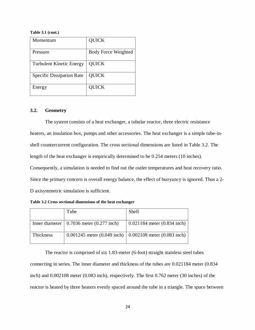
Table 3.1 (cont.)
Momentum QUICK
Pressure Body Force Weighted
Turbulent Kinetic Energy QUICK
Specific Dissipation Rate QUICK
Energy QUICK
3.2. Geometry
The system consists of a heat exchanger, a tubular reactor, three electric resistance
heaters, an insulation box, pumps and other accessories. The heat exchanger is a simple tube-in-
shell countercurrent configuration. The cross sectional dimensions are listed in Table 3.2. The
length of the heat exchanger is empirically determined to be 0.254 meters (10 inches).
Consequently, a simulation is needed to find out the outlet temperatures and heat recovery ratio.
Since the primary concern is overall energy balance, the effect of buoyancy is ignored. Thus a 2-
D axisymmetric simulation is sufficient.
Table 3.2 Cross sectional dimensions of the heat exchanger
Tube Shell
Inner diameter 0.7036 meter (0.277 inch) 0.021184 meter (0.834 inch)
Thickness 0.001245 meter (0.049 inch) 0.002108 meter (0.083 inch)
The reactor is comprised of six 1.83-meter (6-foot) straight stainless steel tubes
connecting in series. The inner diameter and thickness of the tubes are 0.021184 meter (0.834
inch) and 0.002108 meter (0.083 inch), respectively. The first 0.762 meter (30 inches) of the
reactor is heated by three heaters evenly spaced around the tube in a triangle. The space between
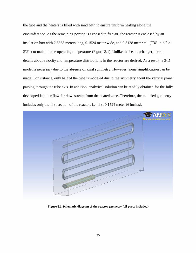
25
the tube and the heaters is filled with sand bath to ensure uniform heating along the
circumference. As the remaining portion is exposed to free air, the reactor is enclosed by an
insulation box with 2.3368 meters long, 0.1524 meter wide, and 0.8128 meter tall (7’8’’ × 6’’ ×
2’8’’) to maintain the operating temperature (Figure 3.1). Unlike the heat exchanger, more
details about velocity and temperature distributions in the reactor are desired. As a result, a 3-D
model is necessary due to the absence of axial symmetry. However, some simplification can be
made. For instance, only half of the tube is modeled due to the symmetry about the vertical plane
passing through the tube axis. In addition, analytical solution can be readily obtained for the fully
developed laminar flow far downstream from the heated zone. Therefore, the modeled geometry
includes only the first section of the reactor, i.e. first 0.1524 meter (6 inches).
Figure 3.1 Schematic diagram of the reactor geometry (all parts included)

26
3.3. Mesh
The 2-D heat exchanger model contains 103,200 rectangular elements. The axial length is
discretized into 2400 divisions. In radial direction, the inner tube and outer tube consist of 3
layers of mesh each, and the cell size of the hot and cold fluid is 0.000254 meter (0.01 inch) with
a growth ratio of 1.25 from the wall (Figure 3.2).
Figure 3.2 Mesh of the heat exchanger (from the top are: shell, cold fluid, tube, and hot fluid)
The 3-D reactor geometry is comprised of 607,090 structured hexahedral elements. In
cross-sections perpendicular to tube axis, there are 40 uniformly spaced cells around the azimuth
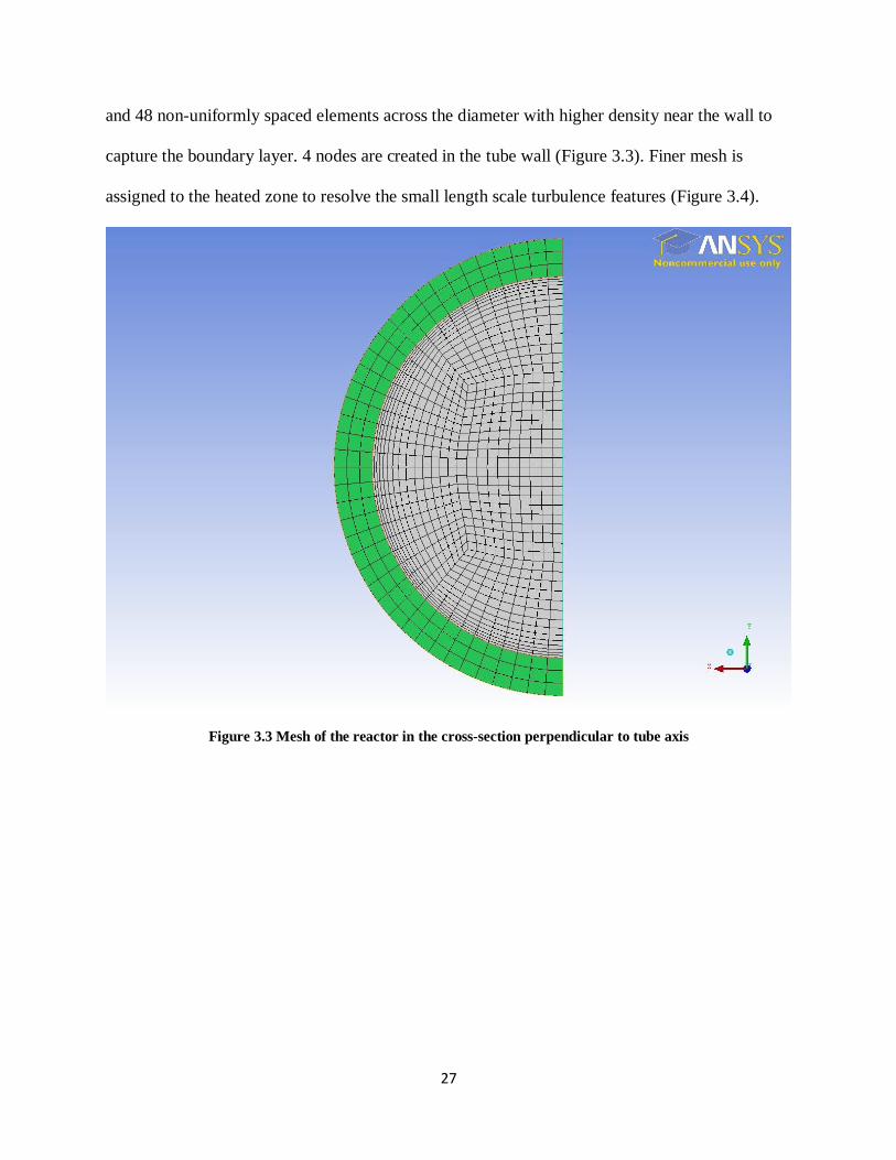
27
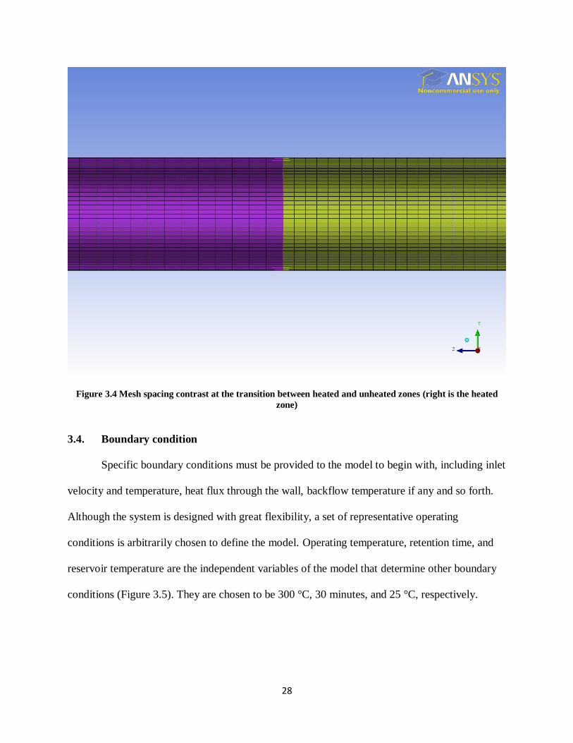
and 48 non-uniformly spaced elements across the diameter with higher density near the wall to
capture the boundary layer. 4 nodes are created in the tube wall (Figure 3.3). Finer mesh is
assigned to the heated zone to resolve the small length scale turbulence features (Figure 3.4).
Figure 3.3 Mesh of the reactor in the cross-section perpendicular to tube axis
28
Figure 3.4 Mesh spacing contrast at the transition between heated and unheated zones (right is the heated
zone)
3.4. Boundary condition
Specific boundary conditions must be provided to the model to begin with, including inlet
velocity and temperature, heat flux through the wall, backflow temperature if any and so forth.
Although the system is designed with great flexibility, a set of representative operating
conditions is arbitrarily chosen to define the model. Operating temperature, retention time, and
reservoir temperature are the independent variables of the model that determine other boundary
conditions (Figure 3.5). They are chosen to be 300 °C, 30 minutes, and 25 °C, respectively.

29
Figure 3.5 Schematic flow chart of the feedstock and product
In order to save computational time, the heaters and the insulation box are excluded from
the model. Instead, the effects of them are approximated by constant and uniform heat flux and
constant free stream temperature convection, respectively. The heat flux value is calculated via
energy balance. The ambient temperature within the box is assumed to be maintained at the
operating temperature.
In order to model hydrodynamically fully developed flow, a pre-simulation is run with
isothermal boundary conditions. The velocity profiles at the outlet are then used as inlet velocity
input in actual simulations. Detailed boundary conditions are presented in Table 3.3.
30
Table 3.3 Boundary conditions of the simulation
Inlet Velocity 0.00757 m/s
Temperature 210 °C
Outlet Gauge pressure 0 Pa
Wall Heat flux 20582 W/m2
3.5. Materials
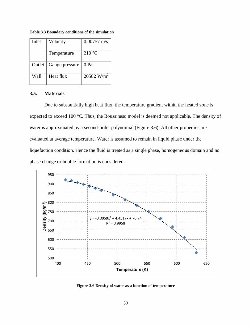
Due to substantially high heat flux, the temperature gradient within the heated zone is
expected to exceed 100 °C. Thus, the Boussinesq model is deemed not applicable. The density of
water is approximated by a second-order polynomial (Figure 3.6). All other properties are
evaluated at average temperature. Water is assumed to remain in liquid phase under the
liquefaction condition. Hence the fluid is treated as a single phase, homogeneous domain and no
phase change or bubble formation is considered.
Figure 3.6 Density of water as a function of temperature
y = -0.0059x2 + 4.4517x + 76.74 R² = 0.9958
500
550
600
650
700
750
800
850
900
950
400 450 500 550 600 650
Den
sit
y (
kg
/m3)
Temperature (K)

31
The property of stainless steel is determined by the default value in ANSYS FLUENT
database.
32
CHAPTER 4
Validation case
The validity of CFD model is assessed by comparison to the results from a frequently
cited reference paper (Mori et al. 1966). A model is designed to exactly replicate the actual
experiment of Mori. The density of air is approximated as a second-order polynomial of
temperature. Other properties are evaluated at average temperature. The geometry is duplicated
from Mori’s experimental setup. A horizontal circular brass tube with 14-meter length, 35.6-
millimeter inner diameter, and 38-millimeter outer diameter is modeled. First 7 meters of the
tube is isothermal and the following 7 meters is uniformly heated. Accordingly, isothermal and
constant heat flux boundary conditions are applied, respectively. The heat flux value is
calculated from the axial temperature gradient in the paper. In addition, the flow rate is computed
by Reynolds number. The mesh contains approximately 1.5 million elements. Detailed model
parameters are listed in table. Simulation results are compared with experimental data in the
literature (Mori et al. 1966).
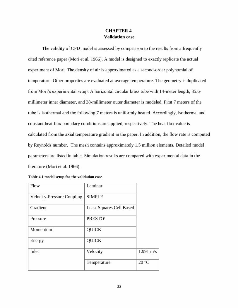
Table 4.1 model setup for the validation case
Flow Laminar
Velocity-Pressure Coupling SIMPLE
Gradient Least Squares Cell Based
Pressure PRESTO!
Momentum QUICK
Energy QUICK
Inlet Velocity 1.991 m/s
Temperature 20 °C

33
Table 4.1 (cont.)
Outlet Gauge pressure 0 Pa
Wall Heat flux 227 W/m2
Figure 4.1 Wall temperature along the axial direction (Mori et al. 1966)
40
60
80
100
120
140
160
0 1 2 3 4 5 6 7
Tw (C
)
Z (m)
Mori et al
CFD
Theoretical

34
Figure 4.2 Dimensionless velocity along vertical center-line at 6 m (Mori et al. 1966)
Figure 4.3 Dimensionless temperature along vertical center-line at 6 m (Mori et al. 1966)
0
0.2
0.4
0.6
0.8
1
1.2
1.4
1.6
-1.2 -1 -0.8 -0.6 -0.4 -0.2 0 0.2 0.4 0.6 0.8 1 1.2
W
y/R
Mori et al
CFD
Poiseuille flow
0
0.2
0.4
0.6
0.8
1
1.2
1.4
1.6
1.8
2
-1.2 -1 -0.8 -0.6 -0.4 -0.2 0 0.2 0.4 0.6 0.8 1 1.2
θ
y/R
Mori et al
CFD
Poiseuille
35
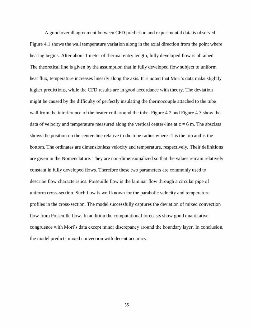
A good overall agreement between CFD prediction and experimental data is observed.
Figure 4.1 shows the wall temperature variation along in the axial direction from the point where
heating begins. After about 1 meter of thermal entry length, fully developed flow is obtained.
The theoretical line is given by the assumption that in fully developed flow subject to uniform
heat flux, temperature increases linearly along the axis. It is noted that Mori’s data make slightly
higher predictions, while the CFD results are in good accordance with theory. The deviation
might be caused by the difficulty of perfectly insulating the thermocouple attached to the tube
wall from the interference of the heater coil around the tube. Figure 4.2 and Figure 4.3 show the
data of velocity and temperature measured along the vertical center-line at z = 6 m. The abscissa
shows the position on the center-line relative to the tube radius where -1 is the top and is the
bottom. The ordinates are dimensionless velocity and temperature, respectively. Their definitions
are given in the Nomenclature. They are non-dimensionalized so that the values remain relatively
constant in fully developed flows. Therefore these two parameters are commonly used to
describe flow characteristics. Poiseuille flow is the laminar flow through a circular pipe of
uniform cross-section. Such flow is well known for the parabolic velocity and temperature
profiles in the cross-section. The model successfully captures the deviation of mixed convection
flow from Poiseuille flow. In addition the computational forecasts show good quantitative
congruence with Mori’s data except minor discrepancy around the boundary layer. In conclusion,
the model predicts mixed convection with decent accuracy.

36
CHAPTER 5
Results and discussion
5.1. Heat exchanger
The temperature profile along the center-line in cold and hot fluids is plotted against the
axial distance (Figure 5.2). After a short entry length, the temperature difference remains
constant, coinciding with the characteristic of countercurrent heat exchangers. The mass flow
average temperatures at the cold fluid outlet and the hot fluid outlet are 212.49 °C and 123.19 °C,
respectively. We define the energy recovery ratio η as the temperature increase of cold fluid
divided by the difference between the operating temperature and the reservoir temperature. The
ratio under current operating condition is 68.18%, a desirable value for a bench scale system. It
is noted that η is also affected by some other factors such as flow rate and temperature.
A series of design points with constant reservoir temperature and varying operating
temperature were also modeled to investigate the optimal condition in terms of energy efficiency.
Figure 5.1 highlighted the exit temperatures of the cold and hot fluids as well as the energy
recovery ratio.

37
Figure 5.1 Outlet temperature and the energy recovery ratio under various operating temperatures
65.0%
66.0%
67.0%
68.0%
69.0%
70.0%
0
50
100
150
200
250
275 280 285 290 295 300 305 310 315 320 325
η
To
ut (°C
)
Top (°C)
cold_out
hot_out
ratio

38
Figure 5.2 Temperature of cold and hot fluids in the heat exchanger along center-lines, respectivley
5.2. Velocity and temperature profiles
The temperature distribution of the tube axis is shown in (Figure 5.3). A thermal entry
length of about 5 inches precedes a linear increase phase followed by a constant temperature
period. Although the inlet temperature is 212.49 °C, identical to cold fluid outlet temperature, the
temperature is increased to 250 °C instantaneously due to the reversed flow. As discussed in
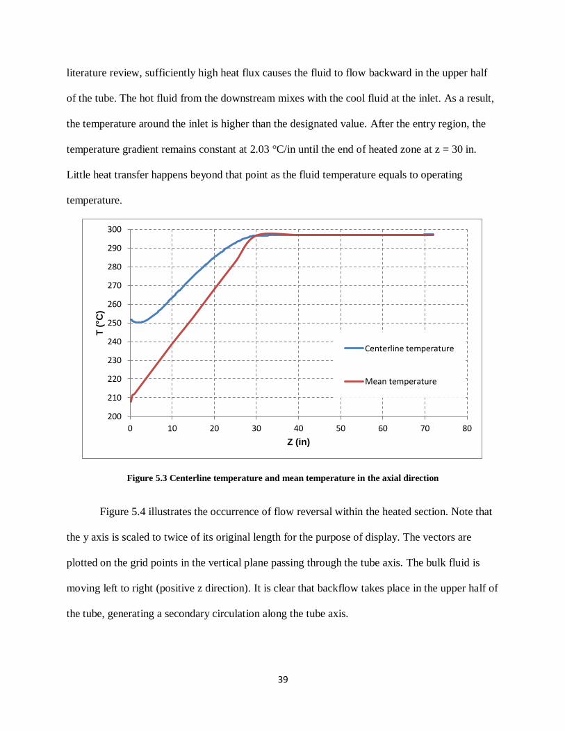
39
literature review, sufficiently high heat flux causes the fluid to flow backward in the upper half
of the tube. The hot fluid from the downstream mixes with the cool fluid at the inlet. As a result,
the temperature around the inlet is higher than the designated value. After the entry region, the
temperature gradient remains constant at 2.03 °C/in until the end of heated zone at z = 30 in.
Little heat transfer happens beyond that point as the fluid temperature equals to operating
temperature.
Figure 5.3 Centerline temperature and mean temperature in the axial direction
Figure 5.4 illustrates the occurrence of flow reversal within the heated section. Note that
the y axis is scaled to twice of its original length for the purpose of display. The vectors are
plotted on the grid points in the vertical plane passing through the tube axis. The bulk fluid is
moving left to right (positive z direction). It is clear that backflow takes place in the upper half of
the tube, generating a secondary circulation along the tube axis.
200
210
220
230
240
250
260
270
280
290
300
0 10 20 30 40 50 60 70 80
T (°C
)
Z (in)
Centerline temperature
Mean temperature

40
Figure 5.4 Velocity vectors in the heated zone from 10 in to 20 in (reversed flow in the upper half)
Figure 5.5 Velocity distributions along the vertical center-line at three locations in the heated zone
-8
-6
-4
-2
0
2
4
6
8
10
-1.2 -1 -0.8 -0.6 -0.4 -0.2 0 0.2 0.4 0.6 0.8 1 1.2
W
y/R
z=10
z=15
z=20
41
The velocity distributions along the vertical center-line are measured at z = 10 in, z = 15
in, and z = 20 in (Figure 5.5). The intensity of reversed flow is the greatest near the inlet and
slightly decreases as the fluid approaches the end of the heated zone where transition to laminar
flow occurs. The velocity profiles are almost identical, indicating fully developed condition.
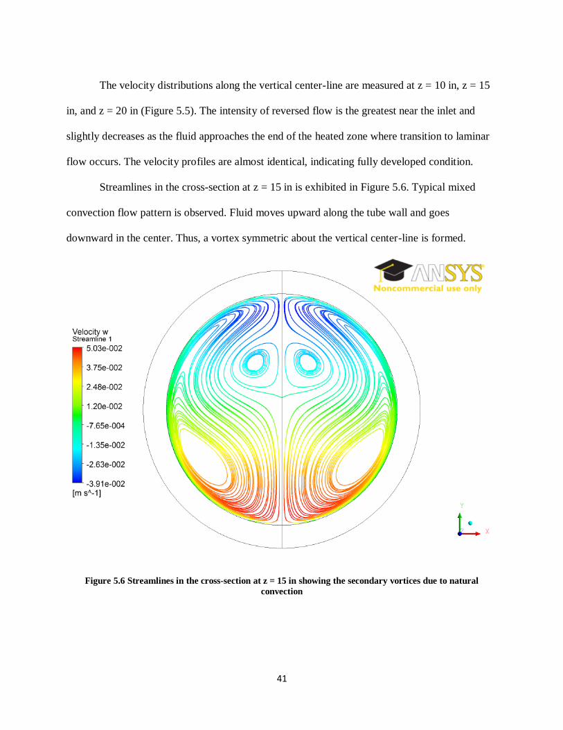
Streamlines in the cross-section at z = 15 in is exhibited in Figure 5.6. Typical mixed
convection flow pattern is observed. Fluid moves upward along the tube wall and goes
downward in the center. Thus, a vortex symmetric about the vertical center-line is formed.
Figure 5.6 Streamlines in the cross-section at z = 15 in showing the secondary vortices due to natural
convection

42
Figure 5.7 demonstrates the temperature contour on the plane passing through the tube
axis in the heated section. Again, the length in y axis is amplified twice. The isotherms
exemplify how the secondary vertex propagates along the tube axis.
Figure 5.7 Temperature contours on symmetric plane in the heated zone from 10 in to 20 in
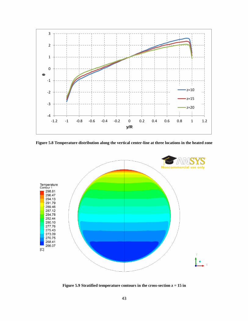
Similarly, temperature distribution measurements are taken at three locations within the
heated zone (Figure 5.8). Unlike the validation case, an evident variation around the
circumference is noticed. Therefore, wall temperature is evaluated as the average of the top and
the bottom values. In spite of its existence, the difference decreases as the fluid gets closer to the
end of the heated section. This trend reveals that the secondary flow induced by buoyancy has a
manifest effect of mitigating the temperature gradient that would be otherwise constant in a flow
under uniform heat flux.
43
Figure 5.8 Temperature distribution along the vertical center-line at three locations in the heated zone
Figure 5.9 Stratified temperature contours in the cross-section z = 15 in
-4
-3
-2
-1
0
1
2
3
-1.2 -1 -0.8 -0.6 -0.4 -0.2 0 0.2 0.4 0.6 0.8 1 1.2
θ
y/R
z=10
z=15
z=20

44
Temperature isotherms are plotted in Figure 5.9 to represent the temperature distribution
in cross sections in the heated zone. Due to the coupling between density and temperature,
stratification occurs. Fluid of the same temperature stays in the same vertical layer. The
phenomenon characterizes the temperature profile of mixed convection flow. In addition, the
rather thin boundary is resultant from the high heat flux.
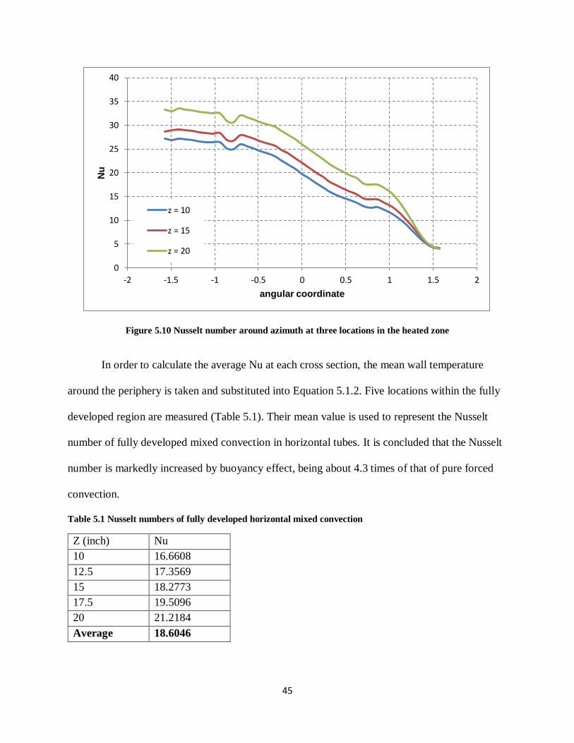
5.3. Nusselt number
Nusselt numbers are computed for both cases using the following equation:
hD
Nuk
(5.1.1)
In the equation, D is tube diameter, k is thermal conductivity of the fluid, and h is heat
transfer coefficient given by:
s w mh q T T (5.1.2)
where sq represents the surface heat flux, and wT and mT are wall and mean temperatures
respectively.
Figure 5.10 show the variation of Nu around the circumference, due to that wall
temperature varies considerably along the azimuth. The vertical axis ranges from 2
to
2
, with
2
being the bottom and
2
representing the top. An obvious trend indicates that the lower half
of the tube is more efficient in heat transfer than the upper half. This phenomenon can be
explained by the fact that both axial velocity and radial velocity are greater in the lower half as
shown in Figure 5.5 and Figure 5.6.
45
Figure 5.10 Nusselt number around azimuth at three locations in the heated zone
In order to calculate the average Nu at each cross section, the mean wall temperature
around the periphery is taken and substituted into Equation 5.1.2. Five locations within the fully
developed region are measured (Table 5.1). Their mean value is used to represent the Nusselt
number of fully developed mixed convection in horizontal tubes. It is concluded that the Nusselt
number is markedly increased by buoyancy effect, being about 4.3 times of that of pure forced
convection.
Table 5.1 Nusselt numbers of fully developed horizontal mixed convection
Z (inch) Nu
10 16.6608
12.5 17.3569
15 18.2773
17.5 19.5096
20 21.2184
Average 18.6046
0
5
10
15
20
25
30
35
40
-2 -1.5 -1 -0.5 0 0.5 1 1.5 2
Nu
angular coordinate
z = 10
z = 15
z = 20

46
5.4. Effect of tube orientation
Identical model parameters are applied to tubes with vertical orientation. However, due to
the alignment between flow direction and buoyancy force, axial symmetry is retained. Therefore,
2-D axisymmetric models are used. It is concluded that in horizontal tubes, natural convection
enhances heat transfer by generating secondary vortex. In vertical tubes, however, buoyancy
force can either assist or diminish heat transfer depending on the direction of the forced flow. For
instance, in upward flows, buoyant motion is in the same direction as the forced motion.
Therefore, natural convection strengthens heat transfer. In downward flows, on the contrary,
buoyancy is in the opposite direction to the bulk fluid motion. Consequently, natural convection
undermines heat transfer.
5.4.1. Velocity and temperature
Figure 5.11 shows the velocity vectors and isotherms for fully developed upward flow.
The average velocity is in positive x-direction while the gravity is applying in the negative x-
direction. Linear increase in temperature indicates the fully developed condition. A thin layer of
thermal boundary layer is identified due to high heat flux. Note that isotherms closely resemble
those of ideal plug-flow. The temperature distribution is almost uniform across the diameter
except the boundary layer, which is extremely desirable in hydrothermal liquefaction kinetics
study.
The flow is concentrated on the near wall region, because buoyant motion greatly
outpaces the forced flow. As a result of continuity, the velocity in the tube central area is
negligible. Reversed flow with limited speed is observed. A more significant flow reversal is
expected if the heat flux is further increased, i.e. stronger natural convection.

47
Figure 5.11 Velocity and temperature distributions in the fully developed region for upward flow
Similar plots are given in Figure 5.12 for fully developed downward flow. Both forced
fluid motion and gravity are in positive x-direction. In contrast to upward flow, significant
reversed flow occurs near the wall, whereas the flow in the center is markedly accelerated due to
mass conservation constraint. Consequently, the temperature variation across the diameter is
magnified.
48
Figure 5.12 Velocity and temperature distributions in the fully developed region for downward flow
5.4.2. Nusselt number
Five points are measured within the fully developed region and the average value is taken
to represent the whole domain. The data are presented in Table 5.2:
Table 5.2 Nusselt numbers of fully developed upward and downward flow
Upward flow Downward flow
z = 10 in 79.26876 26.03742
z = 12.5 in 79.50093 25.45723
z = 15 in 82.20259 25.34986
z = 17.5 in 82.19369 25.29093
z = 20 in 82.06171 25.66505
Average 81.04554 25.5601
It is clear that the Nusselt number of upward flow is significantly larger than that of
downward flow. The relationship concurs with the conclusion that upward flow enhances heat
transfer while downward flow retards it. However, it is worth mentioning that downward flow,
though not as effective as upward flow, improves heat transfer compared to horizontal flow. It is
well known that Nusselt number is a function of Re and Ra. Although the flow is reversed near

49
the wall in downward flow, the velocity magnitude is considerably increased thanks to the
alignment between gravity and velocity, and so are the local Reynolds number and Nusselt
number. In horizontal flow, on the other hand, buoyancy and net flow are orthogonal. Therefore,
the augmentation is relatively insignificant. To test the speculation, we conducted a simulation
identical to that of downward flow except that gravitational acceleration is set 0.01 to reduce
effective Rayleigh number. The Nusselt number is 4.29, lower than that of Poiseuille flow. In
conclusion, downward flow impairs heat transfer at low Ra, while enhances it at high Ra.
5.4.3. Inclined tube
Flows in vertical tubes are distinct with those in horizontal pipes, indicating that tube
orientation has a significant influence on its hydrodynamic and heat transfer characteristics.
Although the analysis has been made for the horizontal case, it is difficult to maintain the tubes
perfectly horizontal. Therefore, additional tests are necessary to investigate the scenario where
the tubes are a few degrees from the horizon. For simplicity, 5° is assumed a reasonable
deviation. All other parameters are identical to previous models. Similarly, upward flow and
downward flow must be discussed separately.
Figure 5.13 and Figure 5.14 show the velocity and temperature profiles along the vertical
centerline at 15 for the inclined tubes in contrast with the horizontal tubes. The velocity profile
for the inclined upward flow is most distinct. The velocity is positive near the wall and
diminishes in the core region. It is because the buoyant force near the wall overcomes the
reversed flow that is seen in the horizontal flow. Despite the difference in velocity profile, the
temperature distribution is similar to that of horizontal tube. On the other hand, the reversed flow
in the upper half in preserved in the inclined downward flow. In addition, its magnitude is
increased to the buoyant force. As a result of the increased velocity magnitude, heat transfer rate

50
is also elevated. Consequently, the temperature profile is slightly more uniform than the other
two cases.
In summary, the velocity and temperature distribution in the tube is sensitive to its
orientation. An inclined angle as small as 5° can cause the profiles to be obviously different than
those of the horizontal case. Hence the tubes should be installed as level as possible to avoid
expected deviation from the model prediction.
Figure 5.13 Velocity profile along the vertical centerline at 15 in for inclined downward, inclined upward, and
horizontal flows
-12
-10
-8
-6
-4
-2
0
2
4
6
8
10
12
-1.2 -1 -0.8 -0.6 -0.4 -0.2 0 0.2 0.4 0.6 0.8 1 1.2
W
y/R
inclined downward
inclinded upward
horizontal

51
Figure 5.14 Temperature profile along the vertical centerline at 15 in for inclined downward, inclined
upward, and horizontal flows
5.5. Residence time distribution
The residence time distribution is obtained for three conditions: constant density, variable
density with 0g , and variable density with 9.81g m/s2. The tracer mass fraction at the outlet
is plotted versus time in Figure 5.15. The red vertical line represents the nominal retention time
3006
s. The figure illustrates that the residence time distribution for all three cases are
qualitatively alike. When density is constant, the peak of the cone falls on the nominal residence
time, indicating that the mean residence time mt is equal to . When density varies with
temperature, the flow is accelerated signified by a considerable forward shift of the cone. The
shift is attributed to continuity, i.e. the decrease in density gives rise to velocity. Therefore, the
fluid emanates faster than it is expected when the axial temperature gradient is large. It is
-3
-2.5
-2
-1.5
-1
-0.5
0
0.5
1
1.5
2
2.5
3
-1.2 -1 -0.8 -0.6 -0.4 -0.2 0 0.2 0.4 0.6 0.8 1 1.2
θ
y/R
inclined downward
inclinded upward
horizontal

52
surprising that buoyant motion does not have a significant impact on the residence time
distribution. The curves of the variable density cases with and without gravity almost completely
overlap. It is likely that residence time distribution characterizes the reactor’s macro-mixing and
is thus primarily determined by the mean velocity rather than velocity distribution. Values of the
parameter pertaining residence time distribution are given in Table 5.3. The mean residence time
is shortened by about 60 seconds because of heating. The inconsistency between the nominal
residence time and the actual residence time will significantly impede the accurate analysis of the
reaction dynamics and mechanism, and must be minimized.
Figure 5.15 Residence time distribution for 6-feet tube
Table 5.3 Residence distribution time parameters
Constant ρ Variable ρ w/o g Variable ρ w/ g
mt (s) 317 246 250
2 58.6 39.6 44.1
3s 5.96 4.15 4.81
0
0.01
0.02
0.03
0.04
0.05
0.06
0 100 200 300 400 500 600
E(t
)
time (s)
τ
constant ρ
variable ρ w/o g
variable ρ w/ g
53
Due to the accelerating effect caused by heating, the flow rate of the pump system must
be corrected to ensure desired residence time. The key to accurate correction is to account for the
variation of velocity with respect to temperature in the heated zone. A simple correction scheme
that assumes linear increase of velocity is proposed. First, the total residence time can be
decomposed as the sum of residence time in the heated zone and constant temperature zone:
CHTOT
H C
LL
v v (5.1.3)
The mean velocity in the heated zone is taken as the arithmetic average of the velocities
at the inlet and outlet of the heated zone:
, ,
2
H in H out
H
v vv
(5.1.4)
It can be derived from mass conservation that the ratio of the velocities between two
cross-sections is the reciprocal of that of the densities which is a known function of temperature:
,
,
( )
( )
H in out
H out in
v T
v T
(5.1.5)
Finally, since velocity remains constant after the heated zone, the outlet velocity of the
heated zone is equal to the velocity of the constant temperature zone:
,H out Cv v (5.1.6)
Inlet velocity ,H inv can then be solved from Equations 5.1.3 through 5.1.6. The RTD of a
new simulation with corrected inlet velocity is compared with the constant density scenario in
Figure 5.16. Notice that the distribution falls much closer to the desirable region with the
proposed correction. The mean residence time is about 295 seconds, less than 5 seconds apart
from the nominal retention time. The correction is effective in predicting the accelerating effect
of density change.

54
Figure 5.16 Residence time distribution with corrected inlet velocity
5.6. Mesh independence study
A mesh with higher grid density is tested under the same model setup to demonstrate that
the original grid is sufficiently fine to produce mesh independent results. The refined mesh
contains 3,118,730 elements. The grid spacing along the tube axis and within the cross-section
perpendicular to the tube axis is both reduced. Dimensionless velocity and temperature profiles
are obtained along the vertical center line at z = 15 in and compared with those of the coarse
mesh (Figure 5.17 and Figure 5.18). The figures show substantial overlapping, indicating that
solution is not improved by further increasing mesh density.
0
0.01
0.02
0.03
0.04
0.05
0 100 200 300 400 500 600
E (
t)
time (s)
constant ρ
variable ρ with correction
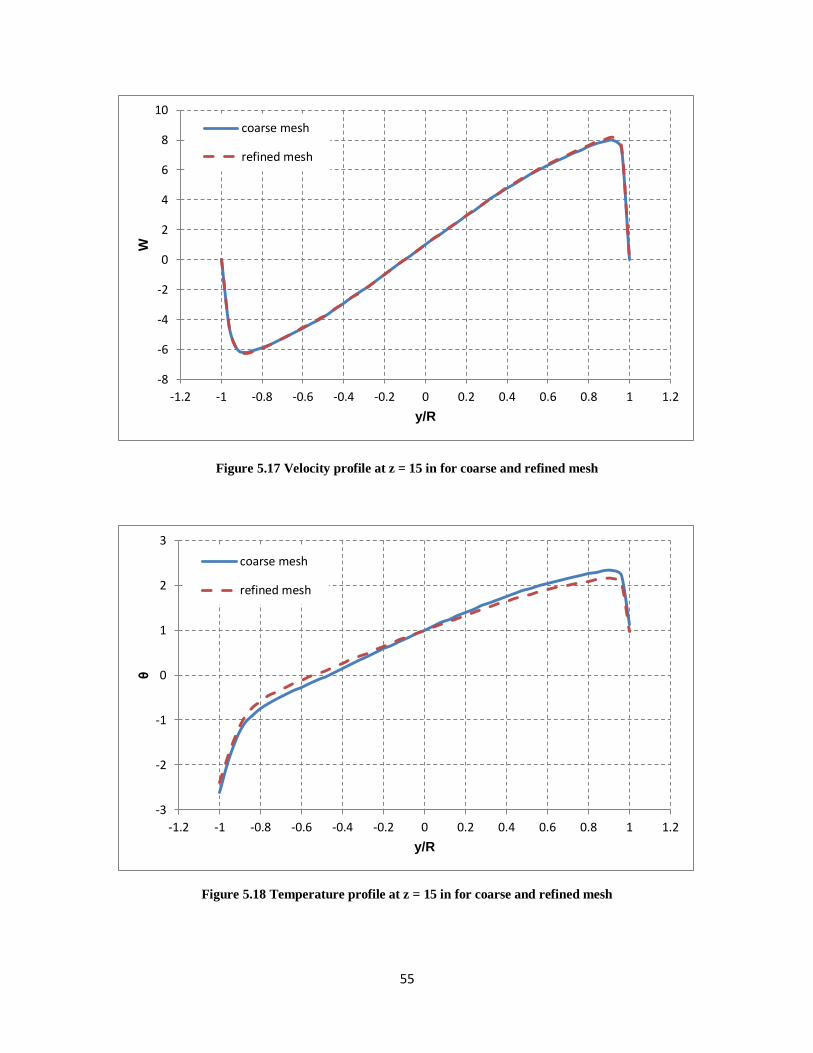
55
Figure 5.17 Velocity profile at z = 15 in for coarse and refined mesh
Figure 5.18 Temperature profile at z = 15 in for coarse and refined mesh
-8
-6
-4
-2
0
2
4
6
8
10
-1.2 -1 -0.8 -0.6 -0.4 -0.2 0 0.2 0.4 0.6 0.8 1 1.2
W
y/R
coarse mesh
refined mesh
-3
-2
-1
0
1
2
3
-1.2 -1 -0.8 -0.6 -0.4 -0.2 0 0.2 0.4 0.6 0.8 1 1.2
θ
y/R
coarse mesh
refined mesh

56
CHAPTER 6
Conclusions and recommendations
6.1. Conclusions
A computational fluid dynamics model is established to study the velocity and
temperature profiles, heat transfer, and residence time distribution within a continuous tubular
hydrothermal liquefaction reactor. The flow regime is best characterized as turbulent combined
forced and natural convection in a horizontal circular tube under uniform heat flux. A detailed
literature review is conducted to provide a survey of relevant research on such flow field. Water
is used as the working medium and its density is approximated as a second-order polynomial
function of temperature to account for the buoyancy term in the governing equation.
In addition, the literature reviews analyzed the transition from laminar flow to turbulence
for a mixed convective flow. It is concluded that hydrodynamic effect and thermal perturbations
are independent of each other. Therefore, the flow regime of the current study is turbulent due to
the substantially high heat flux, despite a Reynolds number that is low. Shear stress transport
k turbulence model is employed given that it includes low-Reynolds-number correction.
The heat exchanger and first segment of the reactor are modeled with 103,200 and
607,090 elements, respectively. The electric resistance heaters surrounding the tube are replaced
by constant heat flux boundary condition; the ambient temperature around the reactor is assumed
to be uniform and constant. Inlet temperature of the cold fluid in the heat exchanger, operating
temperature of the reactor, and retention time are the independent variables of the model. They
are arbitrarily chosen as 25 ºC, 300 ºC, and 30 min to represent a typical HTL reaction. Results
are obtained under such conditions:

57
1. The model is used to simulate a reference case from previous work by Mori et al.
(1966). A good concurrence between the CFD predictions and Mori’s experimental
data is observed.
2. The heat exchanger is able to recover 68.18% of initial energy input that heats the
system to the operating temperature under the current conditions.
3. Both velocity and temperature distributions of mixed convection flow in the modeled
reactor were utterly different than Poiseuille flow. In a cross section perpendicular to
the tube axis, the fluid rises along the wall. The upward currents from both sides of
the wall coincide at the top of the tube and then descend in the central region. The
motion creates two vortices symmetric about the vertical center-line. The temperature
field is stratified with hotter fluid in the higher layers and cooler fluid in the lower
layers. Additionally, temperature varies substantially around the circumference.
4. Marked flow reversal occurs in the upper half of the tube within the heated section.
The intensity of the reversed flow decreases as it approaches the end of the heated
zone.
5. The secondary flow caused by buoyancy significantly enhances heat transfer. The
average Nusselt number in the fully developed region is 18.6. In addition, heat
transfer is more efficient in the lower half of the tube.
6. Tube orientation has a consequential effect on heat transfer rate. Upward flow in a
vertical tube markedly improves heat transfer, whereas downward flow strengthens
heat transfer at high Rayleigh number yet diminishes heat transfer at low Ra.
Amongst the three cases, vertical tube with upward flow is the best scenario in terms

58
of temperature uniformity and heat transfer rate. The temperature contour closely
resembles that of ideal plug-flow.
7. The velocity and temperature profiles are sensitive to tube orientation. A 5° inclined
angle may lead to a vastly different result.
8. The axial temperature gradient accelerates the effluence of the fluid. The mean
residence time is shortened by about 60 seconds. A correction scheme is proposed
and successfully reduced the accelerating effect of temperature gradient to less than 5
seconds.
9. Buoyant motion has little to do with the acceleration of effluent.
6.2. Recommendations
This work creates a platform to assess the performance of the new HTL system.
Nevertheless, the model is an initial attempt built on various assumptions whose validity has yet
to be verified by real experiments. In addition, water is used as a representative medium.
However, the properties of water differ a lot from those of the feedstock. Therefore, the model
may need further modification when applied to algae solution. In summary, the following
recommendations for future research are proposed:
1. The model is validated by another case with different Re and Ra. To better verify the
model, experimental data obtained from the actual system is highly preferable.
2. The physical properties of the feedstock including density, specific heat, thermal
conductivity, and viscosity are vital to applying the model to predicting real operating
conditions.

59
3. Incorporate the model with the control system of the reactor. For instance, since
temperature variation alters the effluent time, a correlation needs to be developed to
help control the pumping system.
4. Test the accuracy of other turbulence models and identify the most suitable one for
this particular application.

60
References
Bergles, A. E. and R. R. Simonds. 1971. Combined forced and free convection for laminar flow
in horizontal tubes with uniform heat flux. International Journal of Heat and Mass Transfer
14(12): 1989-2000.
Brennan, L. and P. Owende. 2010. Biofuels from microalgae—A review of technologies for
production, processing, and extractions of biofuels and co-products. Renewable and Sustainable
Energy Reviews 14(2): 557-577.
Cantrell, K. B., T. Ducey, K. S. Ro and P. G. Hunt. 2008. Livestock waste-to-bioenergy
generation opportunities. Bioresource technology 99(17): 7941-7953.
Cengel, Y. A. 2007. Chapter 8: Internal Forced Convection. In Heat and Mass Transfer: A
Practical Approach, 452. ed. Anonymous , Boston: McGraw-Hill.
Chisti, Y. 2007. Biodiesel from microalgae. Biotechnology Advances 25(3): 294-306.
Dote, Y., S. Sawayama, S. Inoue, T. Minowa and S. Yokoyama. 1994. Recovery of liquid fuel
from hydrocarbon-rich microalgae by thermochemical liquefaction. Fuel 73(12): 1855-1857.
Ede, A. J. 1961. The heat transfer coefficient for flow in a pipe. International Journal of Heat
and Mass Transfer 4(C): 105-110.
El-Hawary, M. A. 1980. EFFECT OF COMBINED FREE AND FORCED CONVECTION ON
THE STABILITY OF FLOW IN A HORIZONTAL TUBE. Journal of Heat Transfer 102(2):
273-278.
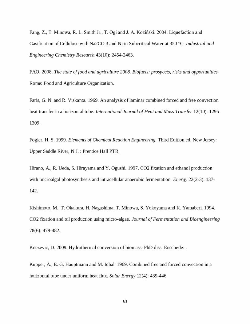
61
Fang, Z., T. Minowa, R. L. Smith Jr., T. Ogi and J. A. Koziński. 2004. Liquefaction and
Gasification of Cellulose with Na2CO 3 and Ni in Subcritical Water at 350 °C. Industrial and
Engineering Chemistry Research 43(10): 2454-2463.
FAO. 2008. The state of food and agriculture 2008. Biofuels: prospects, risks and opportunities.
Rome: Food and Agriculture Organization.
Faris, G. N. and R. Viskanta. 1969. An analysis of laminar combined forced and free convection
heat transfer in a horizontal tube. International Journal of Heat and Mass Transfer 12(10): 1295-
1309.
Fogler, H. S. 1999. Elements of Chemical Reaction Engineering. Third Edition ed. New Jersey:
Upper Saddle River, N.J. : Prentice Hall PTR.
Hirano, A., R. Ueda, S. Hirayama and Y. Ogushi. 1997. CO2 fixation and ethanol production
with microalgal photosynthesis and intracellular anaerobic fermentation. Energy 22(2-3): 137-
142.
Kishimoto, M., T. Okakura, H. Nagashima, T. Minowa, S. Yokoyama and K. Yamaberi. 1994.
CO2 fixation and oil production using micro-algae. Journal of Fermentation and Bioengineering
78(6): 479-482.
Knezevic, D. 2009. Hydrothermal conversion of biomass. PhD diss. Enschede: .
Kupper, A., E. G. Hauptmann and M. Iqbal. 1969. Combined free and forced convection in a
horizontal tube under uniform heat flux. Solar Energy 12(4): 439-446.

62
Metais, B. and E. R. G. Eckert. 1964. Forced, Mixed, and Free Convection Regimes. Journal of
Heat Transfer 86(2): 295-296.
Metting Jr., F. B. 1996. Biodiversity and application of microalgae. Journal of Industrial
Microbiology and Biotechnology 17(5-6): 477-489.
Mikesell, R. D. 1963. The Effect of Heat Transfer on the Flow in a Horizontal Pipe. ProQuest
Dissertations and Theses113 p.
Minowa, T., S. Yokoyama, M. Kishimoto and T. Okakura. 1995. Oil production from algal cells
of Dunaliella tertiolecta by direct thermochemical liquefaction. Fuel 74(12): 1735-1738.
Moore, A. 2008. Biofuels are dead: long live biofuels(?) - Part one. New Biotechnology 25(1): 6-
12.
Mori, Y. and K. Futagami. 1967. Forced convective heat transfer in uniformly heated horizontal
tubes (2nd report, theoretical study). International Journal of Heat and Mass Transfer 10(12):
1801-1804,IN3,1805-1813.
Mori, Y., K. Futagami, S. Tokuda and M. Nakamura. 1966. Forced convective heat transfer in
uniformly heated horizontal tubes 1st report-Experimental study on the effect of buoyancy.
International Journal of Heat and Mass Transfer 9(5): 453-463.
Morton, B. R. 1959. Laminar convection in uniformly heated horizontal pipes at low rayleigh
numbers. Quarterly Journal of Mechanics and Applied Mathematics 12(4): 410-420.
63
Nagendra, H. R. 1973. INTERACTION OF FREE AND FORCED CONVECTION IN
HORIZONTAL TUBES IN THE TRANSITION REGIME. Journal of Fluid Mechanics 57(Part
2): 269-288.
Newell, J.,P.H. and A. E. Bergles. 1970. Analysis of Combined Free and Forced Convection for
Fully Developed Laminar Flow in Horizontal Tubes. Journal of Heat Transfer 92(1): 83-93.
Sawayama, S., T. Minowa and S. Yokoyama. 1999. Possibility of renewable energy production
and CO2 mitigation by thermochemical liquefaction of microalgae. Biomass and Bioenergy
17(1): 33-39.
Sawayama, S., S. Inoue, Y. Dote and S. Yokoyama. 1995. CO2 fixation and oil production
through microalga. Energy Conversion and Management 36(6–9): 729-731.
Schenk, P., S. Thomas-Hall, E. Stephens, U. Marx, J. Mussgnug, C. Posten, O. Kruse and B.
Hankamer. 2008. Second Generation Biofuels: High-Efficiency Microalgae for Biodiesel
Production. BioEnergy Research 1(1): 20-43.
Searchinger, T., R. Heimlich, R. A. Houghton, F. Dong, A. Elobeid, J. Fabiosa, S. Tokgoz, D.
Hayes and T. -. Yu. 2008. Use of U.S. croplands for biofuels increases greenhouse gases through
emissions from land-use change. Science 319(5867): 1238-1240.
Shannon, R. L. and C. A. Depew. 1968. Combined Free and Forced Laminar Convection in a
Horizontal Tube With Uniform Heat Flux. Journal of Heat Transfer 90(3): 353-357.
64
Siegwarth, D. P. and T. J. Hanratty. 1970. Computational and experimental study of the effect of
secondary flow on the temperature field and primary flow in a heated horizontal tube.
International Journal of Heat and Mass Transfer 13(1): 27-42.
Singh, N. K. and D. W. Dhar. 2011. Microalgae as second generation biofuel. A review.
Agronomy for Sustainable Development 31(4): 605-629.
Spolaore, P., C. Joannis-Cassan, E. Duran and A. Isambert. 2006. Commercial applications of
microalgae. Journal of Bioscience and Bioengineering 101(2): 87-96.
USDOE. 2011. Annual Energy Review. 0384.
Wang, M., T. Tsuji and Y. Nagano. 1994. Mixed convection with flow reversal in the thermal
entrance region of horizontal and vertical pipes. International Journal of Heat and Mass
Transfer 37(15): 2305-2319.
Watanabe, M., Y. Aizawa, T. Iida, C. Levy, T. M. Aida and H. Inomata. 2005. Glucose reactions
within the heating period and the effect of heating rate on the reactions in hot compressed water.
Carbohydrate research 340(12): 1931-1939.
Yang, Y. F., C. P. Feng, Y. Inamori and T. Maekawa. 2004. Analysis of energy conversion
characteristics in liquefaction of algae. Resources, Conservation and Recycling 43(1): 21-33.

65
Appendix A
Physical properties of fluids
Table A.1 Properties of saturated water
Temperature
T, °C
Density
ρ, kg/m3
Specific
Heat
Cp, J/(kg·K)
Thermal
Conductivity
k, W/(m·K)
Dynamic
Viscosity
μ, kg/(m·s)
Prandtl
Number
Pr
Volume
Expansion
Coefficient
β, 1/K
0.01 999.8 4217 0.561 1.792×10⁻³
13.5 -0.068×10⁻³
20 998.0 4182 0.598 1.002×10⁻³
7.01 0.195×10⁻³
40 992.1 4179 0.631 0.653×10⁻³
4.32 0.377×10⁻³
60 983.3 4185 0.654 0.467×10⁻³
2.99 0.517×10⁻³
80 971.8 4197 0.670 0.355×10⁻³
2.22 0.653×10⁻³
100 957.9 4217 0.679 0.282×10⁻³
1.75 0.750×10⁻³
120 943.4 4244 0.683 0.232×10⁻³
1.44 0.858×10⁻³
140 921.7 4286 0.683 0.197×10⁻³
1.24 0.970×10⁻³
160 907.4 4340 0.680 0.170×10⁻³
1.09 1.145×10⁻³
180 887.3 4410 0.673 0.150×10⁻³
0.983 1.210×10⁻³
200 864.3 4500 0.663 0.134×10⁻³
0.910 1.350×10⁻³
220 840.3 4610 0.650 0.122×10⁻³
0.865 1.520×10⁻³
240 813.7 4760 0.632 0.111×10⁻³
0.836 1.720×10⁻³
260 783.7 4970 0.609 0.102×10⁻³
0.832 2.000×10⁻³
280 750.8 5280 0.581 0.094×10⁻³
0.854 2.380×10⁻³
300 713.8 5750 0.548 0.086×10⁻³
0.902 2.950×10⁻³
320 667.1 6540 0.509 0.078×10⁻³
1.00 ―
340 610.5 8240 0.469 0.070×10⁻³
1.23 ―
374.14 317.0 ― ― 0.043×10⁻³
― ―

66
Table A.2 Properties of air at 1 atm pressure
Temperature
T, °C
Density
ρ, kg/m3
Specific
Heat
Cp, J/(kg·K)
Thermal
Conductivity
k, W/(m·K)
Dynamic
Viscosity
μ, kg/(m·s)
Prandtl
Number
Pr
0 1.292 1006 0.02364 1.729×10⁻⁵
0.7362
20 1.204 1007 0.02514 1.825×10⁻⁵
0.7309
40 1.127 1007 0.02662 1.918×10⁻⁵
0.7255
60 1.059 1007 0.02808 2.008×10⁻⁵
0.7202
80 0.9994 1008 0.02953 2.096×10⁻⁵
0.7154
100 0.9458 1009 0.03095 2.181×10⁻⁵
0.7111
120 0.8977 1011 0.03235 2.264×10⁻⁵
0.7073
140 0.8542 1013 0.03374 2.345×10⁻⁵
0.7041
160 0.8148 1016 0.03511 2.420×10⁻⁵
0.7014
180 0.7788 1019 0.03646 2.504×10⁻⁵
0.6992
200 0.7459 1023 0.03779 2.577×10⁻⁵
0.6974